Orbits of globular clusters computed with dynamical friction in the Galactic anisotropic velocity dispersion field

Abstract

We present a preliminary analysis of the effect of dynamical friction on the orbits of part of the globular clusters in our Galaxy. Our study considers an anisotropic velocity dispersion field approximated using the results of studies in the literature. An axisymmetric Galactic model with mass components consisting of a disc, a bulge, and a dark halo is employed in the computations. We provide a method to compute the dynamical friction acceleration in ellipsoidal, oblate, and prolate velocity distribution functions with similar density in velocity space. Orbital properties, such as mean time-variations of perigalactic and apogalactic distances, energy, and z-component of angular momentum, are obtained for globular clusters lying in the Galactic region $R\lesssim$ 10 kpc, $|z|\lesssim$ 5 kpc, with $R,z$ cylindrical coordinates. These include clusters in prograde and retrograde orbital motion. Several clusters are strongly affected by dynamical friction, in particular Liller 1, Terzan 4, Terzan 5, NGC 6440, and NGC 6553, which lie in the Galactic inner region. We comment on the more relevant implications of our results on the dynamics of Galactic globular clusters, such as their possible misclassification between the categories ‘halo’, ‘bulge’, and ‘thick disc’, the resulting biasing of globular-cluster samples, the possible incorrect association of the globulars with their parent dwarf galaxies for accretion events, and the possible formation of ‘nuclear star clusters’.

1 Introduction

The acceleration due to dynamical friction on a massive object moving through an infinite, homogeneous stellar medium was obtained by Chandrasekhar (1943), assuming an isotropic velocity dispersion of background stars. Tremaine et al. (1975) employed this result to study the possible formation of nuclei of galaxies when globular clusters spiral into their galactic centre, as they lose orbital energy due to dynamical friction. In our Galaxy, approximating the outer regions with an isotropic velocity dispersion, Tremaine (1976) computed the orbit of the Large Magellanic Cloud under the dynamical friction effect. A detailed study of this effect on the motion of an object with mass 7 $\times 10^{5}$ M_⊙, moving close to the disc of a Galactic potential model, was made by Keenan (1979). He used the ‘representative’ Galactic model of Innanen (1973), taking also constant values of isotropic velocity dispersions in each of the four oblate spheroids representing the disc component in the model.

Employing the general case of an anisotropic velocity dispersion field, several studies analyse the evolution of orbits due to dynamical friction in a given potential. A spherical potential has been considered by Casertano et al. (1987) and Tsuchiya & Shimada (2000). An oblate potential is employed by Surdin & Charikov (1977) and Statler (1988). The motion in triaxial potentials has been studied by Statler (1991) and Pesce et al. (1992). In the present analysis we develop a method to compute the dynamical friction acceleration produced by velocity distribution functions whose constant density surfaces in velocity space are ellipsodal, oblate, or prolate similar surfaces, i.e. they have constant semiaxes ratios. We apply this theory in the disc, bulge, and dark halo of our Galaxy to compute orbits of globular clusters. Recent data obtained by the $Gaia$ mission have increased our understanding of the Galactic kinematics, including in particular the kinematics of the system of globular clusters (Gaia Collaboration et al., 2018a, b), which have been well complemented with large spectroscopic surveys such as APOGEE-2/SDSS-IV (Majewski et al., 2017). From the resulting analysis of these data some new accretion events in our Galaxy have been inferred: Gaia-Sausage (Belokurov et al., 2018), Gaia-Enceladus (Helmi et al., 2018), the possible shards of $\omega$ Centauri (Myeong et al., 2018a), a blob in the nearby stellar halo and a stellar population on highly eccentric orbits (Koppelman et al., 2018; Mackereth et al., 2019), Sequoia (Myeong et al., 2019), Kraken or Koala (Kruijssen et al., 2019, 2020; Forbes, 2020), and a number of chemically anomalous structures associated with the disruption of globular clusters (see, e.g., Fernández-Trincado et al., 2016, 2017b, 2019a, 2019b, 2020a, 2020b, 2020c, 2021b, 2021c, 2021d). These events significantly increase the number of already known events of this type: Sagittarius (Ibata et al., 1994), Helmi Stream (Helmi et al., 1999), Canis Major dwarf galaxy (Martin et al., 2004), a substructure on the Galactic disc (Helmi et al., 2006). All this information has led to the conclusion that some globular clusters have been accreted in these events, and others have been formed in situ (Bellazzini et al., 2003; Forbes & Bridges, 2010; Myeong et al., 2018b; Helmi et al., 2018; Myeong et al., 2019; Massari et al., 2019; Koppelman et al., 2019; Forbes, 2020).

In the process to associate some clusters to a given accretion event, it has been assumed that the orbital energy and $z$-component of the angular momentum are constants, or vary slightly, in time. Under the action of dynamical friction and employing an axisymmetric Galactic potential, these orbital properties are not strictly constant. Thus, the associations cluster-accretion event could be uncertain.

In our analysis of dynamical friction, and in particular for globular clusters whose orbits lie in an inner Galactic region, we quantify the variation of orbital energy and $z$ angular momentum. Our results show that according to the current values of these variations, the assumption of constant orbital properties is approximately appropriate for the majority of studied clusters, except in some cases which show strong variations. However, a further analysis is needed computing the orbits with a backward integration in time, considering an increase of mass of the clusters (Baumgardt et al., 2019). As the acceleration due to dynamical friction depends directly on this mass, the expected greater mass in the past in combination with the decrease of the background density of Galactic regions where the cluster moved, could result in variations of energy and angular momentum similar to the current ones, but some particular clusters deserve a detailed analysis.

This work is organised as follows: In Section 2 and the Appendices, we describe our method to compute the acceleration due to dynamical friction. Section 3 gives the approximated anisotropic velocity dispersion field employed in the computations, using results from the literature. In Section 4, we compute the orbits of globular clusters that lie within a restricted Galactic region. Implications of our results for the system of Galactic globular clusters are commented in Section 5. Our conclusions are given in Section 6.

2 Dynamical friction acceleration

The dynamical-friction acceleration of a body of mass $M$ moving with instantaneous velocity $v$_M with respect to the local velocity centroid, at position $r$, of a system of perturbing particles of mass $m_{\rm p}\ll M$ is (Binney & Tremaine, 2008; Spitzer, 1987)

$$\left(\frac{{\rm d}\mbox{\boldmath$v$}_{M}}{{\rm d}t}\right)_{\rm df}=4{\pi}G^{2}Mm_{\rm p}\ln\Lambda{\nabla}_{\tiny\mbox{\boldmath$v$}_{\tiny\rm M}}h(\mbox{\boldmath$r$},\mbox{\boldmath$v$}_{\rm M}),$$ (1)

with $\ln\Lambda$ the Coulomb logarithm commented below, and $h$($r$,$v$_M) the Rosenbluth potential (Rosenbluth et al., 1957) given by

$$h(\mbox{\boldmath$r$},\mbox{\boldmath$v$}_{\rm M})=\int\frac{f(\mbox{\boldmath$r$},\mbox{\boldmath$v$})}{|\mbox{\boldmath$v$}_{\rm M}-\mbox{\boldmath$v$}|}{d}^{3}\mbox{\boldmath$v$}.$$ (2)

$f$($r$,$v$) is the local distribution function (DF) of particles $m_{\rm p}$, with their velocity $v$ given with respect to their local centroid. The subscript $v$_M in the gradient operator ${\nabla}$ in Eq. 1 denotes derivation in velocity space.

In the acceleration given in Eq. 1, we consider the contribution of particles $m_{\rm p}$ in the three Galactic components: bulge, disc, and dark halo. In each component we assume a local DF of the type

$$f(\mbox{\boldmath$r$},\mbox{\boldmath$v$})=\frac{n}{(2\pi)^{3/2}\sigma_{1}\sigma_{2}\sigma_{3}}\exp\left[-\frac{1}{2}\left(\frac{{v}_{1}^{2}}{\sigma_{1}^{2}}+\frac{{v}_{2}^{2}}{\sigma_{2}^{2}}+\frac{{v}_{3}^{2}}{\sigma_{3}^{2}}\right)\right],$$ (3)

with $n$, $(\sigma_{1},\sigma_{2},\sigma_{3})$, $({v}_{1},{v}_{2},{v}_{3})$ respectively the corresponding local number density, velocity dispersions, and velocity components along the principal axes of the distribution. In our analysis, we consider the general case in which $(\sigma_{1},\sigma_{2},\sigma_{3})$ may be different, i.e. an anisotropic dispersion field. With this DF and defining

$$f_{0}(\mbox{\boldmath$r$},\mbox{\boldmath$v$})=\exp\left[-\frac{1}{2}\left(\frac{{v}_{1}^{2}}{\sigma_{1}^{2}}+\frac{{v}_{2}^{2}}{\sigma_{2}^{2}}+\frac{{v}_{3}^{2}}{\sigma_{3}^{2}}\right)\right],$$ (4)

$${\Psi}(\mbox{\boldmath$r$},\mbox{\boldmath$v$}_{\rm M})=-\int\frac{f_{0}(\mbox{\boldmath$r$},\mbox{\boldmath$v$})}{|\mbox{\boldmath$v$}_{\rm M}-\mbox{\boldmath$v$}|}{d}^{3}\mbox{\boldmath$v$},$$ (5)

then Eq. 1 is

$$\left(\frac{{\rm d}\mbox{\boldmath$v$}_{M}}{{\rm d}t}\right)_{\rm df}=-\sqrt{\frac{2}{\pi}}\frac{G^{2}M\rho_{\rm p}\ln\Lambda}{\sigma_{1}\sigma_{2}\sigma_{3}}{\nabla}_{\tiny\mbox{\boldmath$v$}_{\tiny\rm M}}{\Psi}(\mbox{\boldmath$r$},\mbox{\boldmath$v$}_{\rm M}),$$ (6)

with $\rho_{\rm p}$ the corresponding local mass density of particles $m_{\rm p}$.

The density function $f_{0}$($r$,$v$) is constant on similar ellipsoidal surfaces in velocity space, and can be expressed as a function of an appropriate variable identifying these surfaces. For the computation of the force field $-{\nabla}$${}_{\tiny v_{\rm M}}$${\Psi}$($r$,$v$_M) in Eq. 6, we find it convenient to approximate $f_{0}$ with a series of connected linear segments, which are linear functions of the employed variable. Each linear segment represents a shell in velocity space. In the Appendices A,B,C we present a method to compute in velocity space the force field of a shell of this type, for ellipsoidal: $\sigma_{1}$>$\sigma_{2}$>$\sigma_{3}$, oblate: $\sigma_{1}$=$\sigma_{2}$>$\sigma_{3}$, and prolate: $\sigma_{1}$>$\sigma_{2}$=$\sigma_{3}$ arguments of the function $f_{0}$. In these Appendices the point $v$=$({v}_{1},{v}_{2},{v}_{3})$ represents the velocity $v$_M expressed in the employed Cartesian base ($e$₁,$e$₂,$e$₃)

$$\mbox{\boldmath$v$}_{\tiny\rm M}=\mbox{\boldmath$e$}_{1}{v}_{\rm M1}+\mbox{\boldmath$e$}_{2}{v}_{\rm M2}+\mbox{\boldmath$e$}_{3}{v}_{\rm M3}.$$ (7)

The total field $-{\nabla}$${}_{\tiny v_{\rm M}}$${\Psi}$ at this point $v$_M is obtained with the sum of the individual fields of each shell. As stated in parts (b) and (c) of Appendices A,B,C, the force field inside a shell is zero; thus, in that procedure we take shells only inside the similar surface which crosses the point $v$_M.

In the isotropic case $\sigma_{1}$=$\sigma_{2}$=$\sigma_{3}$=$\sigma$, and with $\gamma$=|$v$_M|$/(\sqrt{2}\sigma)$ we have

$$-{\nabla}_{\tiny\mbox{\boldmath$v$}_{\tiny\rm M}}{\Psi}(\mbox{\boldmath$r$},\mbox{\boldmath$v$}_{\rm M})=-\mbox{\boldmath$v$}_{\rm M}\left(\frac{\sqrt{\pi}}{\gamma}\right)^{3}\left({\rm erf}(\gamma)-\frac{2}{\sqrt{\pi}}\gamma{\rm e}^{-{\gamma}^{2}}\right).$$ (8)

In Section 3, we will take an isotropic bulge component, and assume that at any point $r$ in the dark halo component, the principal axes of the corresponding DF lie along the directions of unitary vectors $e$_r,$e$_φ, $e$_θ in spherical coordinates. In the disc component the principal axes will be taken along the directions of unitary vectors $e$_R,$e$_z,$e$_φ in cylindrical coordinates. Thus, in the dark halo and disc components the corresponding local dispersions $\sigma_{r},\sigma_{\varphi},\sigma_{\theta}$ and $\sigma_{R},\sigma_{z},\sigma_{\varphi}$ are arranged as $\sigma_{1},\sigma_{2},\sigma_{3}$ with $\sigma_{1}$$\geq$$\sigma_{2}$$\geq$$\sigma_{3}$, and set the corresponding right-handed Cartesian base ($e$₁,$e$₂,$e$₃) to be employed in the Appendices A,B,C. In Table 1, we give the possible cases in this arrangement and the assumed base ($e$₁,$e$₂,$e$₃ ). For a given base, the components ${v}_{\rm M1}$,${v}_{\rm M2}$,${v}_{\rm M2}$ in Eq. 7 are obtained assuming that in each Galactic component the velocity of the local centroid with respect to the Galactic inertial frame points in the $e$_φ direction, this velocity being <${v}_{\varphi}$>$e$_φ. Thus, with principal axes in spherical coordinates, if ${V}_{r}$,${V}_{\varphi}$,${V}_{\theta}$ are the components of the velocity $V$ of body $M$ with respect to the Galactic inertial frame, $v$_M for the given Galactic component is

$$\mbox{\boldmath$v$}_{\tiny\rm M}=\mbox{\boldmath$e$}_{r}{V}_{r}+\mbox{\boldmath$e$}_{\varphi}({V}_{\varphi}-<\!{v}_{\varphi}\!>)+\mbox{\boldmath$e$}_{\theta}{V}_{\theta},$$ (9)

and with principal axes in cylindrical coordinates, and ${V}_{R}$,${V}_{z}$,${V}_{\varphi}$ the corresponding components of $V$, the velocity $v$_M is

$$\mbox{\boldmath$v$}_{\tiny\rm M}=\mbox{\boldmath$e$}_{R}{V}_{R}+\mbox{\boldmath$e$}_{z}{V}_{z}+\mbox{\boldmath$e$}_{\varphi}({V}_{\varphi}-<\!{v}_{\varphi}\!>).$$ (10)

In both situations the components ${v}_{\rm M1}$,${v}_{\rm M2}$,${v}_{\rm M3}$ follow inserting a corresponding base ($e$₁,$e$₂,$e$₃) in Eq. 7 from Table 1 and comparing with Eq. 9 or Eq. 10. The total field $-{\nabla}$${}_{\tiny v_{\rm M}}$${\Psi}$ in Eq. 6 is expressed in this base ($e$₁,$e$₂,$e$₃).

With $\Phi$ the total Galactic potential, the instantaneous acceleration of $M$ with respect to the Galactic inertial frame is

$$\frac{{\rm d}\mbox{\boldmath$V$}}{{\rm d}t}=-\nabla\Phi+\sum_{\rm i}\left(\frac{{\rm d}\mbox{\boldmath$v$}_{M}}{{\rm d}t}\right)_{\rm df_{i}},$$ (11)

the second term giving the contributions of the three Galactic components: bulge, disc, and dark halo.

Table 1: Cases in the arrangement of local dispersions.

	spherical		cylindrical
Case	($\sigma_{1},\sigma_{2},\sigma_{3}$)	($e$1, $e$2, $e$3)	($\sigma_{1},\sigma_{2},\sigma_{3}$)	($e$1, $e$2, $e$3)
1	($\sigma_{r},\sigma_{\theta},\sigma_{\varphi}$)	($e$r, $e$θ, $e$φ)	($\sigma_{z},\sigma_{R},\sigma_{\varphi}$)	($e$z, $e$R, $e$φ)
2	($\sigma_{r},\sigma_{\varphi},\sigma_{\theta}$)	($e$r, $e$φ, $-$$e$θ)	($\sigma_{z},\sigma_{\varphi},\sigma_{R}$)	($e$z, $e$φ, $-$$e$R)
3	($\sigma_{\theta},\sigma_{\varphi},\sigma_{r}$)	($e$θ, $e$φ, $e$r)	($\sigma_{R},\sigma_{\varphi},\sigma_{z}$)	($e$R, $e$φ, $e$z)
4	($\sigma_{\theta},\sigma_{r},\sigma_{\varphi}$)	($e$θ, $e$r, $-$$e$φ)	($\sigma_{R},\sigma_{z},\sigma_{\varphi}$)	($e$R, $e$z, $-$$e$φ)
5	($\sigma_{\varphi},\sigma_{r},\sigma_{\theta}$)	($e$φ, $e$r, $e$θ)	($\sigma_{\varphi},\sigma_{z},\sigma_{R}$)	($e$φ, $e$z, $e$R)
6	($\sigma_{\varphi},\sigma_{\theta},\sigma_{r}$)	($e$φ, $e$θ, $-$$e$r)	($\sigma_{\varphi},\sigma_{R},\sigma_{z}$)	($e$φ, $e$R, $-$$e$z)

In the computation of Galactic orbits of globular clusters, following Binney & Tremaine (2008), at every orbital point the factor $\ln\Lambda$ in Eqs. 1, 6 is approximated as

$$\ln\Lambda=\ln\left(\frac{b_{\rm max}}{{\rm max}\left[r_{\rm h},GM/(\sigma_{1}\sigma_{2}\sigma_{3})^{2/3}\right]}\right),$$ (12)

with $r_{\rm h}$ being the half-mass radius of the cluster, and the maximum impact parameter $b_{\rm max}$ is set equal to the instantaneous distance from the cluster to the Galactic Centre.

3 Velocity dispersions and mean rotation velocity of mass components in our Galaxy

To analyse the effect of dynamical friction in our Galaxy, the velocity dispersions and the mean rotation velocity of the mass components are approximated with some studies in the literature. These velocity fields are employed in an axisymmetric Galactic potential model. The considered mass components are a disc, a bulge, and a dark halo; in the following, we summarise some of their properties, along with the Galactic potential. Due to the convenient use in the computations of analytic expressions relating the velocity dispersions and mean rotation velocity with a given position in the Galaxy, we will consider results from the literature, which provide approximately analytic details for these properties in the disc, bulge, and dark halo.

In this preliminary analysis of the effect of dynamical friction, we compute the motion of those globular clusters whose orbits lie within the restricted Galactic region defined approximately by $R\lesssim$ 10 kpc, $|z|\lesssim$ 5 kpc, with $R,z$ cylindrical coordinates. The consideration of this restricted region is due to the approximated velocity dispersions and mean rotation velocity employed in the disc component, whose details are given in the following section. Thus, for the three mass components, we focus on the velocity fields within this region. Future analyses will consider a more extended Galactic region.

3.1 Disc component

The Galactic Disc has been analysed in several studies that include the thin or/and thick discs, e.g. van der Kruit (1988); Lewis & Freeman (1989); Gilmore et al. (1989); van der Kruit & de Grijs (1999); Robin et al. (2003); Bond et al. (2010); Carollo et al. (2010); Spagna et al. (2010); van der Kruit (2010); Lee et al. (2011); van der Kruit & Freeman (2011); Pasetto et al. (2012a, b); Robin et al. (2014); Sharma et al. (2014); Guiglion et al. (2015); Gaia Collaboration et al. (2018a); Nitschai et al. (2020); López-Corredoira et al. (2020); Sharma et al. (2021). In this work, we consider the relations of the form $a+b|z|^{c}$ for the velocity dispersions $\sigma_{R}$,$\sigma_{z}$,$\sigma_{\varphi}$, and mean velocity <${v}_{\varphi}$>, given by Bond et al. (2010); these approximations apply at $R_{0}$, the Galactocentric position of the Sun, and towards the north Galactic Pole. In these relations the value of the distance from the plane, $|z|$, is given in the interval <1,5> kpc, and the dispersions and mean velocity result in ${\rm\,km\,s^{-1}}$. In Table 2 we list the values of the parameters $a,b,c$ given by Bond et al. (2010). In our computations a negative value of <${v}_{\varphi}$> indicates prograde motion, i.e. in the sense of Galactic rotation; see Section 3.4 for the reference frame taken in the computations. Figures 12 and 13 in Guiglion et al. (2015) show that there is no great variation of dispersions and mean velocity in $|z|$ < 1 kpc, thus the relations $a+b|z|^{c}$ of Bond et al. (2010) can be approximately applied towards $z$=0. More detailed relations for $\sigma_{R}$,$\sigma_{z}$ have been given by Sharma et al. (2021), which could be employed in a further analysis.

Following the results obtained by Lewis & Freeman (1989), in cylindrical coordinates $(R,z,\varphi)$ we take for the velocity dispersion $\sigma_{R}(R,z)$ the form

$$\sigma_{R}(R,z)=\sigma_{0}{\rm e}^{-R/2h_{R}}\sigma_{R}(R_{0},z),$$ (13)

with $h_{R}$ being a scale length and $\sigma_{R}(R_{0},z)$ obtained with Table 2. Evaluating at $R_{0}$, this gives

$$\sigma_{R}(R,z)={\rm e}^{-(R-R_{0})/2h_{R}}\sigma_{R}(R_{0},z).$$ (14)

Analogously,

$$\sigma_{z}(R,z)={\rm e}^{-(R-R_{0})/2h_{z}}\sigma_{z}(R_{0},z),$$ (15)

$$\sigma_{\varphi}(R,z)={\rm e}^{-(R-R_{0})/2h_{\varphi}}\sigma_{\varphi}(R_{0},z).$$ (16)

In our computations we take the values $h_{R}$=$h_{z}$=4.37 kpc, $h_{\varphi}$=3.36 kpc given by Lewis & Freeman (1989).

To approximate <${v}_{\varphi}$>$(R,z)$, figure 13 given by Gaia Collaboration et al. (2018a) suggests that we can approximate the rotation velocity at any level $z$ with a Brandt velocity function (Brandt, 1960)

$$V(R)=\frac{3V_{\rm max}\left(\frac{R}{R_{\rm max}}\right)}{1+2\left(\frac{R}{R_{\rm max}}\right)^{3/2}},$$ (17)

with $R_{\rm max}$ the position where the maximum value $V_{\rm max}$ is reached. In terms of $R_{0}$ and the corresponding velocity $V(R_{0})$=<${v}_{\varphi}$>$(R_{0},z)$, the mean rotation velocity is given by

$$<\!{v}_{\varphi}\!>(R,z)=<\!{v}_{\varphi}\!>(R_{0},z)\left(\frac{R}{R_{0}}\right)\frac{1+2\left(\frac{R_{0}}{R_{\rm max}}\right)^{3/2}}{1+2\left(\frac{R}{R_{\rm max}}\right)^{3/2}}.$$ (18)

Figure 13 in Gaia Collaboration et al. (2018a) shows that $R_{\rm max}$ lies approximately in the interval 6–8 kpc; in this work we take $R_{\rm max}$=7 kpc.

According to the results of Bond et al. (2010), for the disc component, we approximate the velocity ellipsoid with principal axes pointing along the directions of unitary vectors in cylindrical coordinates.

Table 2: Parameters $a,b,c$ given by Bond et al. (2010) in the relation $a+b|z|^{c}$ for disc dispersions and mean disc velocity at $R_{0}$ and towards the north Galactic Pole.

	$a$	$b$	$c$
$\sigma_{R}(R_{0},z)$	40	5	1.5
$\sigma_{z}(R_{0},z)$	25	4	1.5
$\sigma_{\varphi}(R_{0},z)$	30	3	2
<${v}_{\varphi}$>$(R_{0},z)$	$-$205	19.2	1.25

3.2 Bulge component

The Galactic Bulge has also several determinations of velocity dispersion and mean rotation velocity, e.g. Freeman et al. (1988); Kent (1992); Ibata & Gilmore (1995); Beaulieu et al. (2000); Howard et al. (2008); Shen et al. (2010); Kunder et al. (2012); Ness et al. (2013); Zoccali et al. (2014); Zasowski et al. (2016); Valenti et al. (2018); Du et al. (2020); Kunder et al. (2020); Zhou et al. (2021). For this component, we take the results given by Zoccali et al. (2014). They find some fits for the radial velocity dispersion $\sigma$ and mean velocity $V$ in terms of Galactic coordinates $(l,b)$. On the Galactic plane their fits in ${\rm\,km\,s^{-1}}$ are

$$\sigma=A_{1}+B_{1}+D_{1}l^{2}+E_{1}{\rm e}^{-l^{2}/s},$$ (19)

$$V=A_{2}+D_{2}\tanh(F_{2}l),$$ (20)

with $A_{1}$=79.39, $B_{1}$=38.45, $D_{1}$=$-$0.26, $E_{1}$=21.08, $s$=2.47, and $A_{2}$=3.8, $D_{2}$=76.7, $F_{2}$=0.3; $l$ in degrees. These values correspond to the projected distance $R_{\perp}=R_{0}\sin l$. In our computations, we approximate as isotropic the dispersion field of the bulge, based on values obtained with Eq. 19. Thus, with $l=\frac{180}{\pi}\arcsin(r/R_{0})$ and $r$ the distance from the Galactic Centre, in spherical coordinates we take

$$\sigma_{r}(r)=\sigma_{\varphi}(r)=\sigma_{\theta}(r)=118-0.26l^{2}+21{\rm e}^{-l^{2}/2.5},$$ (21)

with $r\lesssim 0.363R_{0}$ to avoid negative values.

Ibata & Gilmore (1995), Kunder et al. (2012), and Ness et al. (2013) find that the rotation in the bulge is approximately cylindrical. Thus, with $l=\frac{180}{\pi}\arcsin(R/R_{0})$ and $R$ the cylindrical coordinate, we take

$$<\!{v}_{\varphi}\!>(R)=-77\tanh(0.3l),$$ (22)

here we have ignored the small term $A_{2}$ in Eq. 20, and the minus sign gives a prograde rotation.

3.3 Dark halo component

The Galactic Dark Halo has been studied in short and large distances from the Sun, e.g. Sommer-Larsen et al. (1994, 1997); Chiba & Beers (2000); Battaglia et al. (2005, 2006); Dehnen et al. (2006); Smith et al. (2009); Bond et al. (2010); Carollo et al. (2010); Spagna et al. (2010); Brown et al. (2010); Kafle et al. (2012); Fermani & Schönrich (2013); Kafle et al. (2014); King et al. (2015); Deason et al. (2017); Pérez-Villegas et al. (2017); Bird et al. (2019); Wegg et al. (2019). Here, we consider motions only within its inner region $r\lesssim$ 10 kpc. In this region, Smith et al. (2009) and Bond et al. (2010) give values for velocity dispersions and mean rotation velocity. We take the following values from Bond et al. (2010) as Conditions I, with zero mean rotation: $(\sigma_{r},\sigma_{\varphi},\sigma_{\theta})$=(141,85,75) ${\rm\,km\,s^{-1}}$, <${v}_{\varphi}$>=0.

For Conditions II, from figures 7 and 8 of Wegg et al. (2019) and within the region $R\lesssim$ 10 kpc, $|z|\lesssim$ 5 kpc, we approximate the velocity dispersions and mean prograde rotation velocity with $(\sigma_{r},\sigma_{\varphi},\sigma_{\theta})$=(175,150,125) ${\rm\,km\,s^{-1}}$, <${v}_{\varphi}$>=$-$25 ${\rm\,km\,s^{-1}}$. In these second conditions the non-zero rotation approximates the values $-$37 ${\rm\,km\,s^{-1}}$ given by Spagna et al. (2010), between $-$50 and $-$30 ${\rm\,km\,s^{-1}}$ of Chiba & Beers (2000), and between $-$5 and $-$25 ${\rm\,km\,s^{-1}}$ in Deason et al. (2017).

In this dark halo component, we approximate the velocity ellipsoid with principal axes pointing along the directions of unitary vectors in spherical coordinates (Smith et al., 2009; Bond et al., 2010).

3.4 The Galactic model

The Galactic model employed in our computations is the axisymmetric model of Allen & Santillán (1991). It has three components: a Miyamoto-Nagai (Miyamoto & Nagai, 1975) disc, a spherical bulge, and a spherical dark halo. We rescaled this model to the Sun’s galactocentric distance $R_{0}$=8.15 kpc and Local Standard of Rest velocity of 236 ${\rm\,km\,s^{-1}}$, listed in table 3, column A5 of Reid et al. (2019). The Solar motion, also from this table, is $(U,V,W)_{\odot}$=($-$10.6, 10.7, 7.6)${\rm\,km\,s^{-1}}$, with $U_{\odot}$ negative towards the Galactic Centre. In this model, the computed orbits under the effect of dynamical friction are obtained in an inertial reference frame with origin at the Galactic Centre; the $x$-axis points to the present position of the Sun, and the $y$-axis points in the opposite direction to Galactic rotation. Prograde rotation velocity is in the sense of Galactic rotation, and has a negative sign.

The axisymmetric model of Allen & Santillán (1991) does not include the distinction between the thin and thick discs. Future analyses of the dynamical friction effect will consider the contributions of multiple components belonging to the thin and thick discs, employing the more detailed Galactic model GravPot16 which takes account of these components (Fernández-Trincado, 2017a). A more complete analysis of this effect will be needed in the non-axisymmetric version of this model, which includes a boxy bar and 3D spiral arms.

4 Orbits of globular clusters

As stated in Section 3, we only computed the motion of globular clusters whose orbits lie within the Galactic region $R\lesssim$ 10 kpc, $|z|\lesssim$ 5 kpc, with $R,z$ cylindrical coordinates. With the data of globular clusters from the Holger Baumgardt compilation, we made a first computation of orbits employing the Galactic model in Section 3.4 without the dynamical friction effect, and separated the clusters satisfying the above condition. Table 3 gives the data for these clusters: position, distance from the Sun, heliocentric radial velocity, proper motions, mass, and half-mass radius, all these quantities taken from the Holger Baumgardt compilation. In particular, the mass listed in this table is the current mass of the clusters.

For some clusters in Table 3, and without the dynamical friction effect, in Appendix D we present a comparison of mean perigalactic and apogalactic distances obtained with the Galactic model employed in this work, and corresponding results from Gaia Collaboration et al. (2018b) and the Holger Baumgardt compilation, obtained with Model I of Irrgang et al. (2013), based on the original Galactic model of Allen & Santillán (1991). As shown in Table 8, these perigalactic and apogalactic distances compare well in these similar Galactic models; thus, our results with the dynamical friction effect will represent the orbital evolution under essentially an Allen & Santillán model.

The orbits of all the clusters in Table 3 were computed in a time interval of 5 Gyr in the future, considering the effect of the dynamical friction. Galactic positions and velocities computed with data in this table were taken as initial conditions in the orbits. To test the accuracy of the numerical integration, in some clusters we computed the orbits backwards in time and then forwards in time up to the initial time $t$=0. The initial conditions were recovered with good approximation. In Section 5 we show the orbits of some clusters computed backwards in time, i.e. in the past. As an approximation in all our computations, during the orbital evolution, the mass of a cluster was kept constant and equal to the current value listed in the table. This overestimates the effect of dynamical friction, as shown by Eq. 1, because this mass will decrease with time due to evaporation and tidal shocks, reinforced by dynamical friction itself. Thus, the total integration time of 5 Gyr is only a convenient time to see the trend of the orbital evolution under the maximum dynamical friction effect.

For the computations, we employed the Runge–Kutta algorithm of seventh–eighth order given by Fehlberg (1968). Besides finding the successive orbital perigalactic and apogalactic distances $r_{\rm min}$, $r_{\rm max}$, respectively, we computed at every orbital point the instantaneous values per unit mass of the energy, $E$, the $z$-component of the angular momentum, $L_{z}$, and their time variations $\frac{{\rm d}E}{{\rm d}t}$, $\frac{{\rm d}L_{z}}{{\rm d}t}$. With $V$ the velocity of the cluster with respect to the Galactic inertial frame, and $a$_df the total acceleration due to dynamical friction, i.e. the second term on the right side of Eq. 11, the time variations of $E$ and $L_{z}$ are given by

$$\frac{{\rm d}E}{{\rm d}t}=\mbox{\boldmath$V$}\cdot\mbox{\boldmath$a$}_{\rm df},$$ (23)

$$\frac{{\rm d}L_{z}}{{\rm d}t}=R(a_{\varphi})_{\rm df},$$ (24)

with $(a_{\varphi})_{\rm df}$ the azimutal component of $a$_df.

4.1 Mean variations

As examples, Figs. 1–5 show some orbital properties obtained in selected clusters. We present results mainly using Conditions I in the Galactic dark halo (see Section 3.3); Conditions II give similar results. All the panels in a column correspond to the cluster with the name printed at the top. From top to bottom, the first two panel rows show the meridional orbit, without and with the effect of dynamical friction, respectively in black and red colours. $R$ is distance in cylindrical coordinates. Each orbit is shown in the interval of time given in the corresponding panel; the orbits in red colour are shown in advanced times near 5 Gyr. Details of the orbital evolution are given in the remaining three panels: the third panel row shows as functions of time the values of $r_{\rm min}$ and $r_{\rm max}$, with (red colour) and without (black colour) the effect of dynamical friction. $r$ is distance in spherical coordinates. The last two panel rows give $E$, $L_{z}$ as functions of time, also with the effect of dynamical friction. In these figures the units of $E$ and $L_{z}$ are UE= 10⁵ km² s^-2, UL = 10 kpc km s^-1.

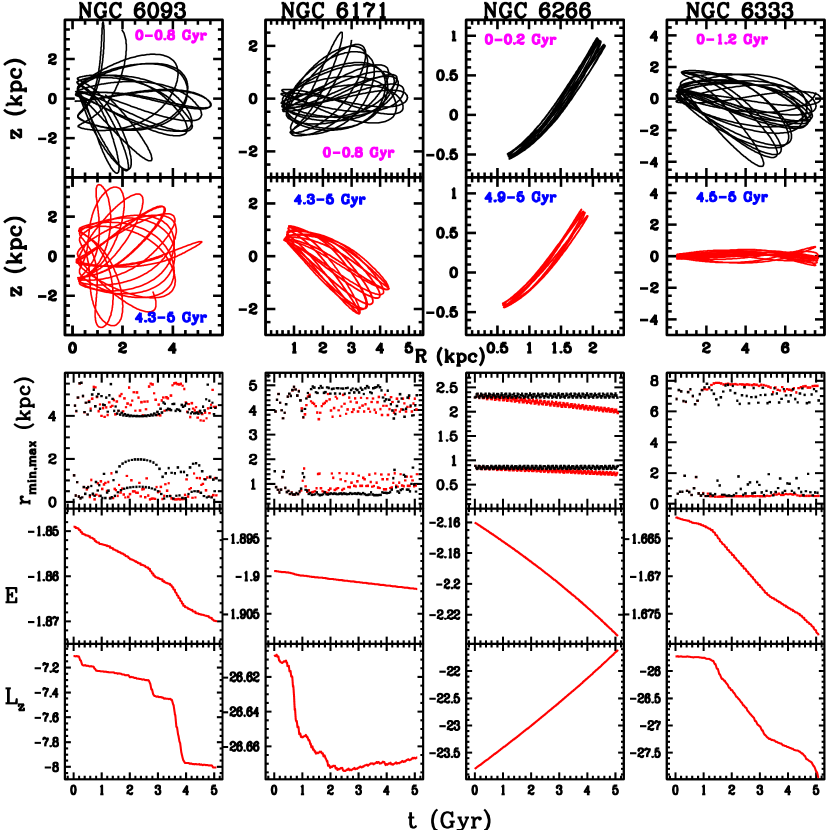
Figure 1: Results for selected clusters. The panels in a column correspond to the cluster with the name printed at the top. From top to bottom, the first two panel rows show the meridional orbit, in the interval of time given in the corresponding panel, without and with the effect of dynamical friction, in black and red colours, respectively. The third panel shows, as functions of time, the values of $r_{\rm min}$ and $r_{\rm max}$, with (red colour) and without (black colour) the effect of dynamical friction. The last two panel rows give $E$, $L_{z}$ as functions of time, also with the effect of dynamical friction. The units of $E$ and $L_{z}$ are UE= 10⁵ km² s^-2, UL = 10 kpc km s^-1.

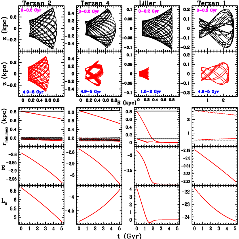
Figure 2: Same as in Fig. 1.

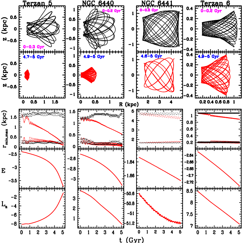
Figure 3: Same as in Fig. 1.

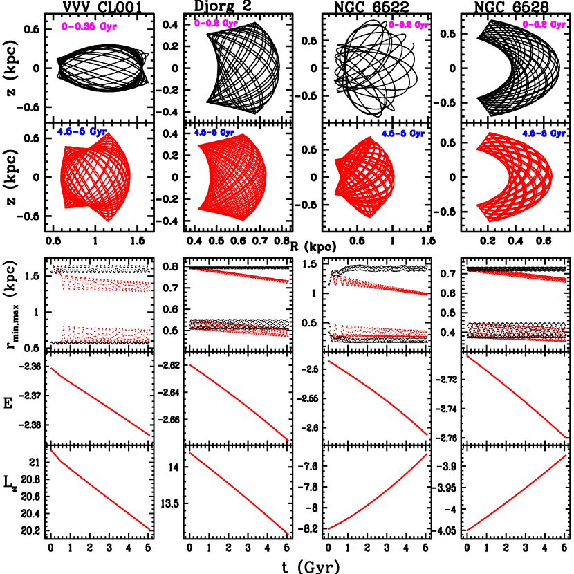
Figure 4: Same as in Fig. 1.

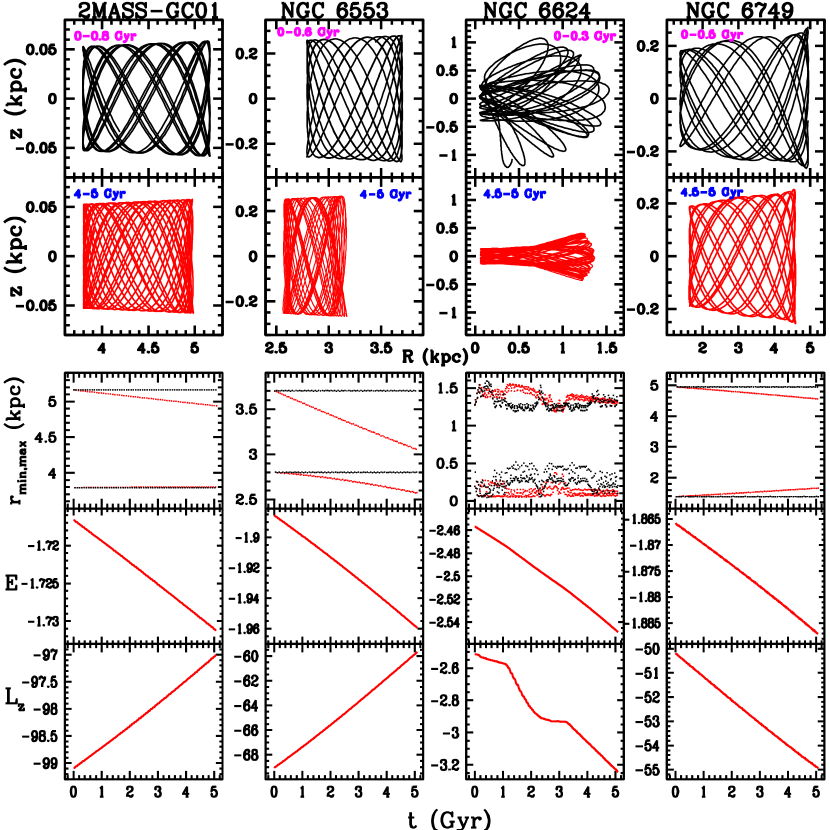
Figure 5: Same as in Fig. 1.

Several orbits in Figs. 1–5 show strong variations in $r_{\rm min}$ and $r_{\rm max}$, particularly the orbit of Liller 1 in Fig. 2, which falls into the Galactic nuclear region in about 2–3 Gyr. Also, in some clusters the mean time-variation of $L_{z}$ is positive, and negative in others. At initial times the orbits of some clusters with and without the effect of dynamical friction can be similar, but they begin to deviate at later times. This behaviour reflects the slight initial effect of dynamical friction in these cases.

In clusters like NGC 6093 and NGC 6171 in Fig. 1 the trend of the mean time-variation of $r_{\rm min}$ and $r_{\rm max}$ is not clearly defined. Thus, we separated the clusters in which these perigalactic and apogalactic time variations could be obtained with reasonable certainty, for example, NGC 6266 in Fig. 1. In this separated sample, we find that $r_{\rm min}$ and $r_{\rm max}$ vary approximately linearly with time over the entire 5 Gyr interval, as shown in some of its members in Figs. 1–5. Thus, with linear least-square fits over this interval we estimated $<\!\dot{r}_{\rm min}\!>$, $<\!\dot{r}_{\rm max}\!>$. In Liller 1 these fits were done only in the first Gyr, due to its rapid later change.

As a result of this linear behaviour, the obtained $<\!\dot{r}_{\rm min}\!>$, $<\!\dot{r}_{\rm max}\!>$ can be applied directly in the first Gyr or early times in the computations, where the assumption of constant mass of the clusters is appropriate. Also, in the separated cluster sample, and in line with the assumption of constant mass, the mean time-variations of energy and angular momentum, $<\!\dot{E}\!>$, $<\!\dot{L}_{z}\!>$, were estimated only over the first Gyr with least-square fits; energy and angular momentum can have different variations in extended time intervals, as shown in Figs. 1–5.

The results of this analysis are listed in Table 5. The initial values $r_{\rm min_{0}}$, $r_{\rm max_{0}}$ are the first perigalactic and apogalactic distances obtained at, or after the start, $t$=0, of an orbital computation, and $E_{0}$, $L_{z_{0}}$ are directly obtained at $t$=0. The last column lists the associated Main Progenitor, given by Massari et al. (2019): cluster formed in situ in the disc (M-D), bulge (M-B), unassociated low energy (L-E), and coming from an accretion event: $Gaia$-Enceladus (G-E), Sequoia (Seq).

Strong variations in $r_{\rm max}$ are obtained in the inner Galaxy clusters Liller 1, Terzan 5, NGC 6440, and NGC 6553. The first three clusters have an initial angular momentum $L_{z_{0}}$ of low magnitude. Terzan 2 and Terzan 4, also with low $L_{z_{0}}$, have a slightly smaller variation in $r_{\rm max}$. NGC 5139 (Omega Centauri) has moderate to strong variations in $r_{\rm min}$, $r_{\rm max}$.

The values of $<\!\dot{r}_{\rm min}\!>$, $<\!\dot{r}_{\rm max}\!>$ in Table 5 are in units of pc Gyr^-1, which in some clusters can be quite small, mainly in $<\!\dot{r}_{\rm min}\!>$. Their corresponding listed uncertainties can be of the same order of the mean values, but even without the effect of dynamical friction, and so under $E$, $L_{z}$ constant, some clusters can present strong variations of $r_{\rm min}$, $r_{\rm max}$, e.g. NGC 6093 in Fig. 1. The uncertainties in the mean time-variations were estimated computing the orbits with initial minimum and maximum energies in each cluster, considering the effect of dynamical friction, according to the uncertainties in distance, radial velocity, and proper motions listed in Table 3; Moreno et al. (2014) find that this procedure gives uncertainty estimates that approximates those obtained with a Monte Carlo simulation.

In the clusters not included in Table 5, we computed only the mean time-variations $<\!\dot{E}\!>$, $<\!\dot{L}_{z}\!>$ by means of linear least-squares fits, taking the time interval of the first Gyr. These variations, along with $r_{\rm min_{0}}$, $r_{\rm max_{0}}$, $E_{0}$, $L_{z_{0}}$ are listed in Table 6. The symbols indicating progenitors shown in this table are as in Table 5; the new symbol K stands for the $Koala$ dwarf galaxy accretion event (Forbes, 2020). In the old, metal-deficient, cluster VVV CL001, not listed by Massari et al. (2019) and Forbes (2020), a possible association with Sequoia or Gaia-Enceladus structures has been suggested by Fernández-Trincado et al. (2021a), and this is listed in Table 6. Fig. 4 shows a moderate effect of dynamical friction in this cluster. Also, in a recent study, based on the age-metallicity relation, Pal 6 is shown to be connected with the M-B group (Souza et al., 2021), instead of the L-E group proposed by Massari et al. (2019). For the strongly affected clusters Terzan 4, Terzan 5, NGC6440, and NGC 6553, Massari et al. (2019) provide an in situ bulge origin, but the extreme effect of dynamical friction in these cases requires a future detailed analysis of these clusters, including Liller 1 with uncertain classification by Massari et al..

Table 3: Globular clusters with orbits lying in the Galactic region $R\lesssim$ 10 kpc, $|z|\lesssim$ 5 kpc.

Cluster	$\alpha$	$\delta$	$r$	$v_{r}$	$\mu_{x}$	$\mu_{y}$	$M_{c}$	$r_{h}$
	(deg)	(deg)	(kpc)	(${\rm\,km\,s^{-1}}$)	(mas yr-1)	(mas yr-1)	($M_{\sun}$)	(pc)
NGC 104	6.023792	$-$72.081306	4.52$\pm$0.03	$-$17.45$\pm$0.16	5.252$\pm$0.021	$-$2.551$\pm$0.021	8.95$\times 10^{5}$	6.30
NGC 4372	186.439101	$-$72.659084	5.71$\pm$0.21	75.59$\pm$0.30	$-$6.409$\pm$0.024	3.297$\pm$0.024	1.98$\times 10^{5}$	8.53
BH 140	193.472915	$-$67.177276	4.81$\pm$0.25	90.30$\pm$0.35	$-$14.848$\pm$0.024	1.224$\pm$0.024	5.99$\times 10^{4}$	9.53
NGC 4833	194.891342	$-$70.876503	6.48$\pm$0.08	201.99$\pm$0.40	$-$8.377$\pm$0.025	$-$0.963$\pm$0.025	2.06$\times 10^{5}$	4.76
NGC 5139	201.696991	$-$47.479473	5.43$\pm$0.05	232.78$\pm$0.21	$-$3.341$\pm$0.028	$-$6.557$\pm$0.043	3.64$\times 10^{6}$	10.36
NGC 5927	232.002869	$-$50.673031	8.27$\pm$0.11	$-$104.09$\pm$0.28	$-$5.056$\pm$0.025	$-$3.217$\pm$0.025	2.75$\times 10^{5}$	5.28
NGC 5946	233.869051	$-$50.659713	9.64$\pm$0.51	137.60$\pm$0.94	$-$5.331$\pm$0.028	$-$1.657$\pm$0.027	9.31$\times 10^{4}$	2.59
NGC 5986	236.512497	$-$37.786415	10.54$\pm$0.13	101.18$\pm$0.43	$-$4.192$\pm$0.026	$-$4.568$\pm$0.026	3.34$\times 10^{5}$	4.25
FSR 1716	242.625000	$-$53.748889	7.43$\pm$0.27	$-$30.70$\pm$0.98	$-$4.354$\pm$0.033	$-$8.832$\pm$0.031	6.43$\times 10^{4}$	5.16
Lynga 7	242.765213	$-$55.317776	7.90$\pm$0.16	17.86$\pm$0.83	$-$3.851$\pm$0.027	$-$7.050$\pm$0.027	7.96$\times 10^{4}$	5.16
NGC 6093	244.260040	$-$22.976084	10.34$\pm$0.12	10.93$\pm$0.39	$-$2.934$\pm$0.027	$-$5.578$\pm$0.026	3.38$\times 10^{5}$	2.62
NGC 6121	245.896744	$-$26.525749	1.85$\pm$0.02	71.21$\pm$0.15	$-$12.514$\pm$0.023	$-$19.022$\pm$0.023	8.71$\times 10^{4}$	3.69
NGC 6144	246.807770	$-$26.023500	8.15$\pm$0.13	194.79$\pm$0.58	$-$1.744$\pm$0.026	$-$2.607$\pm$0.026	7.92$\times 10^{4}$	4.91
NGC 6139	246.918466	$-$38.848782	10.04$\pm$0.45	24.41$\pm$0.95	$-$6.081$\pm$0.027	$-$2.711$\pm$0.026	3.23$\times 10^{5}$	2.47
Terzan 3	247.162483	$-$35.339829	7.64$\pm$0.31	$-$135.76$\pm$0.57	$-$5.577$\pm$0.027	$-$1.760$\pm$0.026	4.04$\times 10^{4}$	7.19
NGC 6171	248.132752	$-$13.053778	5.63$\pm$0.08	$-$34.71$\pm$0.18	$-$1.939$\pm$0.025	$-$5.979$\pm$0.025	7.49$\times 10^{4}$	3.94
ESO 452-SC11	249.854167	$-$28.399167	7.39$\pm$0.20	16.37$\pm$0.44	$-$1.423$\pm$0.031	$-$6.472$\pm$0.030	8.26$\times 10^{3}$	3.68
NGC 6218	251.809067	$-$1.948528	5.11$\pm$0.05	$-$41.67$\pm$0.14	$-$0.191$\pm$0.024	$-$6.802$\pm$0.024	1.07$\times 10^{5}$	4.05
FSR 1735	253.044174	$-$47.058056	9.08$\pm$0.53	$-$69.85$\pm$4.88	$-$4.439$\pm$0.054	$-$1.534$\pm$0.048	7.23$\times 10^{4}$	2.97
NGC 6235	253.355676	$-$22.177447	11.94$\pm$0.38	126.68$\pm$0.33	$-$3.931$\pm$0.027	$-$7.587$\pm$0.027	1.07$\times 10^{5}$	4.78
NGC 6254	254.287720	$-$4.100306	5.07$\pm$0.06	74.21$\pm$0.23	$-$4.758$\pm$0.024	$-$6.597$\pm$0.024	2.05$\times 10^{5}$	4.81
NGC 6256	254.886107	$-$37.120968	7.24$\pm$0.29	$-$99.75$\pm$0.66	$-$3.715$\pm$0.031	$-$1.637$\pm$0.030	1.25$\times 10^{5}$	4.82
NGC 6266	255.304153	$-$30.113390	6.41$\pm$0.10	$-$73.98$\pm$0.67	$-$4.978$\pm$0.026	$-$2.947$\pm$0.026	6.10$\times 10^{5}$	2.43
NGC 6273	255.657486	$-$26.267971	8.34$\pm$0.16	145.54$\pm$0.59	$-$3.249$\pm$0.026	1.660$\pm$0.025	6.97$\times 10^{5}$	4.21
NGC 6284	256.120114	$-$24.764799	14.21$\pm$0.42	28.62$\pm$0.73	$-$3.200$\pm$0.029	$-$2.002$\pm$0.028	1.29$\times 10^{5}$	3.78
NGC 6287	256.288904	$-$22.708005	7.93$\pm$0.37	$-$294.74$\pm$1.65	$-$5.010$\pm$0.029	$-$1.883$\pm$0.028	1.45$\times 10^{5}$	3.65
NGC 6293	257.542500	$-$26.582083	9.19$\pm$0.28	$-$143.66$\pm$0.39	0.870$\pm$0.028	$-$4.326$\pm$0.028	2.05$\times 10^{5}$	4.05
NGC 6304	258.634399	$-$29.462028	6.15$\pm$0.15	$-$108.62$\pm$0.39	$-$4.070$\pm$0.029	$-$1.088$\pm$0.028	1.26$\times 10^{5}$	4.26
NGC 6316	259.155417	$-$28.140111	11.15$\pm$0.39	99.65$\pm$0.84	$-$4.969$\pm$0.031	$-$4.592$\pm$0.030	3.18$\times 10^{5}$	4.77
NGC 6325	259.496327	$-$23.767677	7.53$\pm$0.32	29.54$\pm$0.58	$-$8.289$\pm$0.030	$-$9.000$\pm$0.029	5.89$\times 10^{4}$	2.05
NGC 6333	259.799086	$-$18.516257	8.30$\pm$0.14	310.75$\pm$2.12	$-$2.180$\pm$0.026	$-$3.222$\pm$0.026	3.23$\times 10^{5}$	4.17
NGC 6342	260.291573	$-$19.587659	8.01$\pm$0.23	115.75$\pm$0.90	$-$2.903$\pm$0.027	$-$7.116$\pm$0.026	4.22$\times 10^{4}$	2.06
NGC 6356	260.895804	$-$17.813027	15.66$\pm$0.92	48.18$\pm$1.82	$-$3.750$\pm$0.026	$-$3.392$\pm$0.026	6.00$\times 10^{5}$	6.86
NGC 6355	260.993533	$-$26.352827	8.65$\pm$0.22	$-$195.85$\pm$0.55	$-$4.738$\pm$0.031	$-$0.572$\pm$0.030	1.01$\times 10^{5}$	3.55
NGC 6352	261.371277	$-$48.422169	5.54$\pm$0.07	$-$125.63$\pm$1.01	$-$2.158$\pm$0.025	$-$4.447$\pm$0.025	6.47$\times 10^{4}$	4.56
Terzan 2	261.887917	$-$30.802333	7.75$\pm$0.33	134.56$\pm$0.96	$-$2.170$\pm$0.041	$-$6.263$\pm$0.038	1.36$\times 10^{5}$	4.16
NGC 6366	261.934357	$-$5.079861	3.44$\pm$0.05	$-$120.65$\pm$0.19	$-$0.332$\pm$0.025	$-$5.160$\pm$0.024	3.76$\times 10^{4}$	5.56
Terzan 4	262.662506	$-$31.595528	7.59$\pm$0.31	$-$48.96$\pm$1.57	$-$5.462$\pm$0.060	$-$3.711$\pm$0.048	2.00$\times 10^{5}$	6.06
HP 1	262.771667	$-$29.981667	7.00$\pm$0.14	39.76$\pm$1.22	2.523$\pm$0.039	$-$10.093$\pm$0.037	1.24$\times 10^{5}$	3.74
NGC 6362	262.979096	$-$67.048332	7.65$\pm$0.07	$-$14.58$\pm$0.18	$-$5.506$\pm$0.024	$-$4.763$\pm$0.024	1.27$\times 10^{5}$	7.23
Liller 1	263.352333	$-$33.389556	8.06$\pm$0.34	60.36$\pm$2.44	$-$5.403$\pm$0.109	$-$7.431$\pm$0.077	9.15$\times 10^{5}$	2.01
NGC 6380	263.618611	$-$39.069530	9.61$\pm$0.30	$-$1.48$\pm$0.73	$-$2.183$\pm$0.031	$-$3.233$\pm$0.030	3.34$\times 10^{5}$	4.40
Terzan 1	263.946667	$-$30.481778	5.67$\pm$0.17	56.75$\pm$1.61	$-$2.806$\pm$0.055	$-$4.861$\pm$0.055	1.50$\times 10^{5}$	2.15
Ton 2	264.039293	$-$38.540925	6.99$\pm$0.34	$-$184.72$\pm$1.12	$-$5.904$\pm$0.031	$-$0.755$\pm$0.029	6.91$\times 10^{4}$	4.60
NGC 6388	264.071777	$-$44.735500	11.17$\pm$0.16	83.11$\pm$0.45	$-$1.316$\pm$0.026	$-$2.709$\pm$0.026	1.25$\times 10^{6}$	4.34
NGC 6402	264.400651	$-$3.245916	9.14$\pm$0.25	$-$60.71$\pm$0.45	$-$3.590$\pm$0.025	$-$5.059$\pm$0.025	5.92$\times 10^{5}$	5.14
NGC 6401	264.652191	$-$23.909605	8.06$\pm$0.24	$-$105.44$\pm$2.50	$-$2.748$\pm$0.035	1.444$\pm$0.034	1.45$\times 10^{5}$	3.28
NGC 6397	265.175385	$-$53.674335	2.48$\pm$0.02	18.51$\pm$0.08	3.260$\pm$0.023	$-$17.664$\pm$0.022	9.66$\times 10^{4}$	3.90
Pal 6	265.925812	$-$26.224995	7.05$\pm$0.45	177.00$\pm$1.35	$-$9.222$\pm$0.038	$-$5.347$\pm$0.036	9.45$\times 10^{4}$	2.89
Djorg 1	266.869583	$-$33.066389	9.88$\pm$0.65	$-$359.18$\pm$1.64	$-$4.693$\pm$0.046	$-$8.468$\pm$0.041	7.97$\times 10^{4}$	5.57
Terzan 5	267.020200	$-$24.779055	6.62$\pm$0.15	$-$82.57$\pm$0.73	$-$1.989$\pm$0.068	$-$5.243$\pm$0.066	9.35$\times 10^{5}$	3.77
NGC 6440	267.220167	$-$20.360417	8.25$\pm$0.24	$-$69.39$\pm$0.93	$-$1.187$\pm$0.036	$-$4.020$\pm$0.035	4.89$\times 10^{5}$	2.14
NGC 6441	267.554413	$-$37.051445	12.73$\pm$0.16	18.47$\pm$0.56	$-$2.551$\pm$0.028	$-$5.348$\pm$0.028	1.32$\times 10^{6}$	3.47
Terzan 6	267.693250	$-$31.275389	7.27$\pm$0.35	136.45$\pm$1.50	$-$4.979$\pm$0.048	$-$7.431$\pm$0.039	1.04$\times 10^{5}$	1.33
NGC 6453	267.715508	$-$34.598477	10.07$\pm$0.22	$-$99.23$\pm$1.24	0.203$\pm$0.036	$-$5.934$\pm$0.037	1.65$\times 10^{5}$	3.85
UKS 1	268.613312	$-$24.145277	15.58$\pm$0.56	59.38$\pm$2.63	$-$2.040$\pm$0.095	$-$2.754$\pm$0.063	7.70$\times 10^{4}$	3.84
VVV CL001	268.677083	$-$24.014722	8.08$\pm$1.48	$-$327.28$\pm$0.90	$-$3.487$\pm$0.144	$-$1.652$\pm$0.107	1.35$\times 10^{5}$	2.94
NGC 6496	269.765350	$-$44.265945	9.64$\pm$0.15	$-$134.72$\pm$0.26	$-$3.060$\pm$0.027	$-$9.271$\pm$0.026	6.89$\times 10^{4}$	6.42
Terzan 9	270.411667	$-$26.839722	5.77$\pm$0.34	68.49$\pm$0.56	$-$2.121$\pm$0.052	$-$7.763$\pm$0.049	1.20$\times 10^{5}$	1.90
Djorg 2	270.454378	$-$27.825819	8.76$\pm$0.18	$-$149.75$\pm$1.10	0.662$\pm$0.042	$-$2.983$\pm$0.037	1.25$\times 10^{5}$	5.16
NGC 6517	270.460750	$-$8.958778	9.23$\pm$0.56	$-$35.06$\pm$1.65	$-$1.551$\pm$0.029	$-$4.470$\pm$0.028	1.95$\times 10^{5}$	2.29
Terzan 10	270.740833	$-$26.066944	10.21$\pm$0.40	211.37$\pm$2.27	$-$6.827$\pm$0.059	$-$2.588$\pm$0.050	3.02$\times 10^{5}$	4.60

Table 4: continued

Cluster	$\alpha$	$\delta$	$r$	$v_{r}$	$\mu_{x}$	$\mu_{y}$	$M_{c}$	$r_{h}$
	(deg)	(deg)	(kpc)	(${\rm\,km\,s^{-1}}$)	(mas yr-1)	(mas yr-1)	($M_{\sun}$)	(pc)
NGC 6522	270.891977	$-$30.033974	7.29$\pm$0.21	$-$15.23$\pm$0.49	2.566$\pm$0.039	$-$6.438$\pm$0.036	2.11$\times 10^{5}$	3.08
NGC 6535	270.960449	$-$0.297639	6.36$\pm$0.12	$-$214.85$\pm$0.46	$-$4.214$\pm$0.027	$-$2.939$\pm$0.026	2.19$\times 10^{4}$	3.65
NGC 6528	271.206697	$-$30.055778	7.83$\pm$0.24	211.86$\pm$0.43	$-$2.157$\pm$0.043	$-$5.649$\pm$0.039	5.67$\times 10^{4}$	2.73
NGC 6539	271.207276	$-$7.585858	8.16$\pm$0.39	35.19$\pm$0.50	$-$6.896$\pm$0.026	$-$3.537$\pm$0.026	2.09$\times 10^{5}$	5.18
NGC 6540	271.535657	$-$27.765286	5.91$\pm$0.27	$-$16.50$\pm$0.78	$-$3.702$\pm$0.032	$-$2.791$\pm$0.032	3.45$\times 10^{4}$	5.32
NGC 6544	271.833833	$-$24.998222	2.58$\pm$0.06	$-$38.46$\pm$0.67	$-$2.304$\pm$0.031	$-$18.604$\pm$0.030	9.14$\times 10^{4}$	2.07
NGC 6541	272.009827	$-$43.714889	7.61$\pm$0.10	$-$163.97$\pm$0.46	0.287$\pm$0.025	$-$8.847$\pm$0.025	2.93$\times 10^{5}$	4.34
2MASS-GC01	272.090851	$-$19.829723	3.37$\pm$0.62	$-$31.28$\pm$0.50	$-$1.121$\pm$0.296	$-$1.881$\pm$0.235	3.50$\times 10^{4}$	4.70
NGC 6553	272.315322	$-$25.907750	5.33$\pm$0.13	$-$0.27$\pm$0.34	0.344$\pm$0.030	$-$0.454$\pm$0.029	2.85$\times 10^{5}$	4.56
2MASS-GC02	272.402100	$-$20.778889	5.50$\pm$0.44	$-$237.75 $\pm$10.10	4.000$\pm$0.900	$-$4.700$\pm$0.800	1.60$\times 10^{4}$	2.85
NGC 6558	272.573974	$-$31.764508	7.47$\pm$0.29	$-$195.12$\pm$0.73	$-$1.720$\pm$0.036	$-$4.144$\pm$0.034	2.65$\times 10^{4}$	1.70
IC 1276	272.684441	$-$7.207595	4.55$\pm$0.25	155.06$\pm$0.69	$-$2.553$\pm$0.026	$-$4.568$\pm$0.026	7.39$\times 10^{4}$	5.21
Terzan 12	273.065833	$-$22.741944	5.17$\pm$0.38	95.61$\pm$1.21	$-$6.222$\pm$0.037	$-$3.052$\pm$0.034	8.72$\times 10^{4}$	3.28
NGC 6569	273.411667	$-$31.826889	10.53$\pm$0.26	$-$49.83$\pm$0.50	$-$4.125$\pm$0.028	$-$7.354$\pm$0.028	2.36$\times 10^{5}$	3.85
BH 261	273.527500	$-$28.635000	6.12$\pm$0.26	$-$45.00$\pm$15.00	3.566$\pm$0.043	$-$3.590$\pm$0.037	2.20$\times 10^{4}$	4.66
NGC 6624	275.918793	$-$30.361029	8.02$\pm$0.11	54.79$\pm$0.40	0.124$\pm$0.029	$-$6.936$\pm$0.029	1.56$\times 10^{5}$	3.69
NGC 6626	276.137039	$-$24.869847	5.37$\pm$0.10	11.11$\pm$0.60	$-$0.278$\pm$0.028	$-$8.922$\pm$0.028	2.99$\times 10^{5}$	2.26
NGC 6638	277.733734	$-$25.497473	9.78$\pm$0.34	8.63$\pm$2.00	$-$2.518$\pm$0.029	$-$4.076$\pm$0.029	1.18$\times 10^{5}$	2.20
NGC 6637	277.846252	$-$32.348084	8.90$\pm$0.10	47.48$\pm$1.00	$-$5.034$\pm$0.028	$-$5.832$\pm$0.028	1.55$\times 10^{5}$	3.69
NGC 6642	277.975957	$-$23.475602	8.05$\pm$0.20	$-$60.61$\pm$1.35	$-$0.173$\pm$0.030	$-$3.892$\pm$0.030	3.44$\times 10^{4}$	1.51
NGC 6652	278.940125	$-$32.990723	9.46$\pm$0.14	$-$95.37$\pm$0.86	$-$5.484$\pm$0.027	$-$4.274$\pm$0.027	4.81$\times 10^{4}$	1.96
NGC 6656	279.099762	$-$23.904749	3.30$\pm$0.04	$-$148.72$\pm$0.78	9.851$\pm$0.023	$-$5.617$\pm$0.023	4.76$\times 10^{5}$	5.29
Pal 8	280.377290	$-$19.828858	11.32$\pm$0.63	$-$31.54$\pm$0.21	$-$1.987$\pm$0.027	$-$5.694$\pm$0.027	6.74$\times 10^{4}$	5.86
NGC 6681	280.803162	$-$32.292110	9.36$\pm$0.11	216.62$\pm$0.84	1.431$\pm$0.027	$-$4.744$\pm$0.026	1.16$\times 10^{5}$	2.89
NGC 6712	283.268021	$-$8.705960	7.38$\pm$0.24	$-$107.45$\pm$0.29	3.363$\pm$0.027	$-$4.436$\pm$0.027	9.63$\times 10^{4}$	3.21
NGC 6717	283.775177	$-$22.701473	7.52$\pm$0.13	30.25$\pm$0.90	$-$3.125$\pm$0.027	$-$5.008$\pm$0.027	3.58$\times 10^{4}$	4.23
NGC 6723	284.888123	$-$36.632248	8.27$\pm$0.10	$-$94.39$\pm$0.26	1.028$\pm$0.025	$-$2.418$\pm$0.025	1.77$\times 10^{5}$	5.06
NGC 6749	286.314056	1.899756	7.59$\pm$0.21	$-$58.44$\pm$0.96	$-$2.829$\pm$0.028	$-$6.006$\pm$0.027	2.11$\times 10^{5}$	7.09
NGC 6752	287.717102	$-$59.984554	4.12$\pm$0.04	$-$26.01$\pm$0.12	$-$3.161$\pm$0.022	$-$4.027$\pm$0.022	2.76$\times 10^{5}$	5.27
NGC 6760	287.800268	1.030466	8.41$\pm$0.43	$-$2.37$\pm$1.27	$-$1.107$\pm$0.026	$-$3.615$\pm$0.026	2.69$\times 10^{5}$	5.22
NGC 6809	294.998779	$-$30.964750	5.35$\pm$0.05	174.70$\pm$0.17	$-$3.432$\pm$0.024	$-$9.311$\pm$0.024	1.93$\times 10^{5}$	6.95
Pal 11	296.310000	$-$8.007222	14.02$\pm$0.51	$-$67.64$\pm$0.76	$-$1.766$\pm$0.030	$-$4.971$\pm$0.028	1.19$\times 10^{4}$	7.72
NGC 6838	298.443726	18.779194	4.00$\pm$0.05	$-$22.72$\pm$0.20	$-$3.416$\pm$0.025	$-$2.656$\pm$0.024	4.57$\times 10^{4}$	5.23
NGC 7078	322.493042	12.167001	10.71$\pm$0.10	$-$106.84$\pm$0.30	$-$0.659$\pm$0.024	$-$3.803$\pm$0.024	6.33$\times 10^{5}$	4.30

Table 5: Orbital properties of globular clusters that have approximately well defined perigalactic and apogalactic mean time-variations $<\!\dot{r}_{\rm min}\!>$, $<\!\dot{r}_{\rm max}\!>$, here determined over 5 Gyr. In Liller 1 only the first Gyr is considered. The mean time-variations of energy and angular momentum, $<\!\dot{E}\!>$, $<\!\dot{L}_{z}\!>$, are determined over 1 Gyr. Units of $E$ and $L_{z}$ are UE=10⁵ km² s^-2, UL=10 kpc km s^-1. The clusters are listed in order of increasing right ascension.

Cluster	$r_{\rm min_{0}}$	$r_{\rm max_{0}}$	$<\!\dot{r}_{\rm min}\!>$	$<\!\dot{r}_{\rm max}\!>$	$E_{0}$	$<\!\dot{E}\!>$	$L_{z_{0}}$	$<\!\dot{L}_{z}\!>$	Progenitor
	(kpc)	(kpc)	(pc Gyr-1)	(pc Gyr-1)	(UE)	($10^{-3}$UE Gyr-1)	(UL)	(UL Gyr-1)
NGC 5139	1.87	6.72	$-30\pm 16$	$-76\pm 15$	$-$1.65	$-6.27\pm 0.07$	52.2	$-0.955\pm 0.003$	G-E/Seq
NGC 6266	0.89	2.29	$-26\pm 2$	$-62\pm 7$	$-$2.16	$-12.32\pm 1.6$	$-$23.8	0.387$\pm 0.003$	M-B
Terzan 2	0.17	0.81	$-8\pm 4$	$-36\pm 2$	$-$2.79	$-29.76\pm 9.5$	6.7	$-0.344\pm 0.08$	M-B
Terzan 4	0.16	0.84	$-4\pm 5$	$-59\pm 7$	$-$2.77	$-45.55\pm 21$	$-$4.9	0.149$\pm 0.05$	M-B
Liller 1	0.094	0.81	$-69\pm 8$	$-359\pm 60$	$-$2.84	$-418.60\pm 130$	4.2	$-3.406\pm 1.7$
Terzan 1	0.49	2.64	23$\pm 6$	$-66\pm 12$	$-$2.19	$-7.66\pm 1.56$	$-$21.7	$-0.756\pm 0.17$	M-B
Terzan 5	0.19	1.71	$-38\pm 3$	$-259\pm 64$	$-$2.40	$-78.11\pm 37$	$-$8.1	0.107$\pm 0.25$	M-B
NGC 6440	0.31	1.27	$-28\pm 10$	$-142\pm 13$	$-$2.51	$-60.67\pm 11$	3.8	$-0.436\pm 0.12$	M-B
NGC 6441	1.68	4.84	24$\pm 3$	$-91\pm 7$	$-$1.83	$-6.46\pm 0.1$	$-$50.6	$-0.195\pm 0.015$	L-E
Djorg 2	0.51	0.80	$-8\pm 2$	$-13\pm 5$	$-$2.62	$-10.03\pm 7.7$	14.2	$-0.209\pm 0.08$	M-B
2MASS-GC01	3.79	5.16	2$\pm 5$	$-44\pm 4$	$-$1.72	$-2.81\pm 0.1$	$-$99.1	0.381$\pm 0.12$
NGC 6553	2.80	3.70	$-45\pm 2$	$-128\pm 5$	$-$1.89	$-13.45\pm 0.2$	$-$69.1	1.687$\pm 0.1$	M-B
IC 1276	3.66	7.22	8$\pm 2$	$-19\pm 2$	$-$1.59	$-0.70\pm 0.02$	$-$111.2	$-0.039\pm 0.02$	M-D
NGC 6749	1.38	4.95	55$\pm 3$	$-77\pm 6$	$-$1.87	$-3.92\pm 0.1$	$-$50.2	$-0.974\pm 0.04$	M-D
NGC 6760	1.86	5.78	24$\pm 2$	$-48\pm 3$	$-$1.76	$-2.44\pm 0.22$	$-$63.4	$-0.362\pm 0.01$	M-D
NGC 6838	4.86	7.08	3$\pm 2$	$-17\pm 2$	$-$1.54	$-0.70\pm 0.01$	$-$132.8	0.098$\pm 0.01$	M-D

Table 6: Orbital properties of globular clusters not included in Table 5. The mean time-variations $<\!\dot{E}\!>$, $<\!\dot{L}_{z}\!>$ are determined over the first Gyr. Units are those given in Table 5.

Cluster	$r_{\rm min_{0}}$	$r_{\rm max_{0}}$	$E_{0}$	$<\!\dot{E}\!>$	$L_{z_{0}}$	$<\!\dot{L}_{z}\!>$	Progenitor	Cluster	$r_{\rm min_{0}}$	$r_{\rm max_{0}}$	$E_{0}$	$<\!\dot{E}\!>$	$L_{z_{0}}$	$<\!\dot{L}_{z}\!>$	Progenitor
NGC 104	5.91	7.51	$-$1.46	$-$0.554	$-$124.1	0.117	M-D	NGC 6401	0.38	1.33	$-$2.46	$-$12.011	1.9	$-$0.060	K
NGC 4372	2.91	7.22	$-$1.60	$-$0.501	$-$90.4	$-$0.008	M-D	NGC 6397	2.26	6.28	$-$1.66	$-$0.164	$-$65.1	0.004	M-D
BH 140	1.97	10.19	$-$1.49	$-$0.349	$-$81.1	$-$0.045		Pal 6	0.60	1.80	$-$2.25	$-$3.322	2.1	$-$0.043	M-B
NGC 4833	0.51	8.02	$-$1.63	$-$0.821	$-$23.6	$-$0.033	G-E	Djorg 1	1.18	10.28	$-$1.50	$-$0.320	$-$53.7	$-$0.038	G-E
NGC 5927	4.22	5.68	$-$1.64	$-$2.333	$-$107.7	0.372	M-D	Terzan 6	0.19	1.08	$-$2.63	$-$18.257	8.5	$-$0.293	M-B
NGC 5946	0.19	5.32	$-$1.82	$-$0.731	$-$4.6	$-$0.016	K	NGC 6453	0.67	2.14	$-$2.12	$-$5.100	$-$5.8	$-$0.126	K
NGC 5986	1.37	5.05	$-$1.80	$-$2.518	$-$13.8	$-$0.062	K	UKS 1	0.18	8.09	$-$1.65	$-$0.583	$-$11.5	$-$0.035
FSR 1716	2.41	5.02	$-$1.78	$-$0.245	$-$65.6	0.004	M-D	VVV CL001	0.58	1.56	$-$2.36	$-$5.016	21.1	$-$0.224	G-E/Seq
Lynga 7	1.72	4.54	$-$1.86	$-$0.474	$-$51.3	$-$0.018	M-D	NGC 6496	2.45	5.29	$-$1.72	$-$0.118	$-$61.9	0.004	M-D
NGC 6093	1.23	4.48	$-$1.85	$-$4.088	$-$7.1	$-$0.137	K	Terzan 9	0.23	2.65	$-$2.20	$-$3.774	$-$12.2	$-$0.004	M-B
NGC 6121	0.46	6.45	$-$1.75	$-$0.692	$-$23.8	$-$0.064	L-E	NGC 6517	0.63	3.29	$-$2.04	$-$3.637	$-$12.3	$-$0.070	K
NGC 6144	2.08	3.30	$-$1.88	$-$0.197	16.6	$-$0.012	K	Terzan 10	0.80	5.71	$-$1.74	$-$1.069	$-$20.6	0.005	G-E
NGC 6139	0.92	3.69	$-$1.91	$-$1.354	$-$26.0	0.009	K	NGC 6522	0.33	1.15	$-$2.49	$-$21.569	$-$8.2	0.100	M-B
Terzan 3	2.26	3.04	$-$1.91	$-$0.114	$-$45.2	0.011	M-D	NGC 6535	0.98	4.58	$-$1.88	$-$0.093	30.3	$-$0.009	Seq
NGC 6171	1.52	3.94	$-$1.90	$-$0.648	$-$26.6	$-$0.053	M-B	NGC 6528	0.38	0.73	$-$2.70	$-$10.157	$-$4.1	0.032	M-B
ESO 452-SC11	0.26	2.81	$-$2.16	$-$0.321	$-$1.8	$-$0.010		NGC 6539	1.77	3.40	$-$1.87	$-$0.468	$-$33.0	0.025	M-B
NGC 6218	2.49	4.79	$-$1.76	$-$0.207	$-$46.9	0.009	M-D	NGC 6540	0.86	2.30	$-$2.18	$-$0.859	$-$28.9	0.024	M-B
FSR 1735	1.09	3.83	$-$1.93	$-$0.426	$-$33.2	0.008	K	NGC 6544	0.43	5.60	$-$1.82	$-$0.959	$-$17.1	$-$0.046	K
NGC 6235	3.10	8.56	$-$1.48	$-$0.085	$-$76.7	0.010	G-E	NGC 6541	1.51	3.68	$-$1.89	$-$0.840	$-$32.8	0.028	K
NGC 6254	1.59	4.60	$-$1.79	$-$0.412	$-$42.0	0.016	K	2MASS-GC02	0.80	6.28	$-$1.74	$-$0.068	$-$21.2	$-$0.001
NGC 6256	1.31	2.11	$-$2.14	$-$2.540	$-$34.3	0.169	K	NGC 6558	0.51	1.26	$-$2.43	$-$1.836	$-$6.2	0.006	M-B
NGC 6273	0.81	3.29	$-$1.93	$-$3.416	7.3	$-$0.100	K	Terzan 12	1.62	3.69	$-$1.94	$-$0.728	$-$47.0	0.005	M-D
NGC 6284	0.23	6.58	$-$1.66	$-$0.713	6.6	$-$0.013	G-E	NGC 6569	1.76	2.83	$-$2.00	$-$1.583	$-$40.1	0.116	M-B
NGC 6287	0.23	4.48	$-$1.85	$-$0.978	$-$2.9	$-$0.014	K	BH 261	1.69	2.97	$-$1.99	$-$0.142	$-$39.9	0.010	M-B
NGC 6293	0.20	2.65	$-$2.09	$-$2.881	6.7	$-$0.047	M-B	NGC 6624	0.19	1.28	$-$2.46	$-$15.451	$-$2.5	$-$0.057	M-B
NGC 6304	1.45	2.67	$-$2.06	$-$1.482	$-$38.1	0.094	M-B	NGC 6626	0.33	3.11	$-$2.09	$-$5.939	$-$15.3	$-$0.036	M-B
NGC 6316	1.15	3.91	$-$1.94	$-$1.995	$-$26.5	0.047	M-B	NGC 6638	0.58	2.33	$-$2.19	$-$5.011	$-$2.5	$-$0.043	M-B
NGC 6325	0.94	1.31	$-$2.28	$-$0.973	12.5	$-$0.027	M-B	NGC 6637	0.59	1.98	$-$2.23	$-$5.298	$-$6.0	$-$0.026	M-B
NGC 6333	0.67	6.81	$-$1.66	$-$1.079	$-$25.7	$-$0.026	K	NGC 6642	0.35	1.84	$-$2.32	$-$2.561	1.7	$-$0.040	M-B
NGC 6342	0.61	1.69	$-$2.24	$-$0.873	$-$9.5	0.006	M-B	NGC 6652	0.26	3.34	$-$2.04	$-$1.106	$-$2.6	$-$0.011	M-B
NGC 6356	3.71	8.98	$-$1.46	$-$0.475	$-$93.3	0.055	M-D	NGC 6656	3.10	9.79	$-$1.46	$-$0.698	$-$93.7	0.060	M-D
NGC 6355	0.76	1.25	$-$2.31	$-$1.879	3.9	$-$0.025	M-B	Pal 8	1.20	4.19	$-$1.91	$-$0.337	$-$34.8	0.008	M-D
NGC 6352	3.12	4.12	$-$1.81	$-$0.681	$-$75.2	0.091	M-D	NGC 6681	1.82	5.15	$-$1.76	$-$1.141	0.2	$-$0.033	K
NGC 6366	2.07	5.79	$-$1.72	$-$0.127	$-$64.4	$-$0.003	M-D	NGC 6712	0.29	4.74	$-$1.85	$-$1.375	1.6	$-$0.057	K
HP 1	0.82	1.60	$-$2.27	$-$2.716	0.4	$-$0.018	M-B	NGC 6717	0.86	2.53	$-$2.13	$-$0.634	$-$19.5	0.005	M-B
NGC 6362	3.13	5.27	$-$1.69	$-$0.154	$-$56.5	0.012	M-D	NGC 6723	2.56	2.62	$-$1.91	$-$0.448	$-$4.3	$-$0.006	M-B
NGC 6380	0.20	2.32	$-$2.26	$-$13.088	5.8	$-$0.283	M-B	NGC 6752	3.66	5.49	$-$1.67	$-$0.501	$-$83.3	0.055	M-D
Ton 2	1.74	2.85	$-$1.98	$-$0.384	$-$39.8	0.022	K	NGC 6809	1.57	5.66	$-$1.70	$-$0.337	$-$23.0	0.003	K
NGC 6388	1.11	4.08	$-$1.93	$-$5.750	32.5	$-$0.543	M-B	Pal 11	4.94	8.66	$-$1.44	$-$0.008	$-$121.7	0.001	M-D
NGC 6402	0.49	4.68	$-$1.91	$-$5.233	$-$14.8	$-$0.082	K	NGC 7078	4.12	10.74	$-$1.38	$-$0.467	$-$110.8	0.060	M-D

With data from Tables 5 and 6, in Fig. 6 we show how the clusters are distributed in the plane ($L_{z_{0}}$,$E_{0}$), their positive or negative mean time-variation $<\!\dot{L}_{z}\!>$ over the first Gyr, and their distribution in initial orbital eccentricities. In panel (a) the points with red colour correspond to clusters with positive $<\!\dot{L}_{z}\!>$, and those in blue colour, to clusters with negative $<\!\dot{L}_{z}\!>$. All the clusters with retrograde motion, i.e. $L_{z_{0}}$ > 0, have $<\!\dot{L}_{z}\!>$ negative, which means that their magnitude of angular momentum $L_{z}$ is decreasing. Clusters with prograde motion, i.e. $L_{z_{0}}$ < 0, can have $<\!\dot{L}_{z}\!>$ positive or negative. Those with positive $<\!\dot{L}_{z}\!>$ have a decreasing magnitude of $L_{z}$, and those with negative $<\!\dot{L}_{z}\!>$ have an increasing magnitude of $L_{z}$. The black curves shown in this panel represent prograde and retrograde circular orbits in the axisymmetric Galactic potential. In panel (b), we show again all the points in panel (a), now marked with a green cross the points corresponding to clusters that have an initial eccentricity, $e_{0}$, less than 0.6. We define $e_{0}=(r_{\rm max_{0}}-r_{\rm min_{0}})/(r_{\rm max_{0}}+r_{\rm min_{0}})$. Practically all the clusters with positive $<\!\dot{L}_{z}\!>$, i.e. the red points in panel (a), have $e_{0}$ < 0.6. This approximate value depends on the given definition of $e_{0}$, which relates perigalactic and apogalactic distances around the current time. Another definition of $e_{0}$ could be $e_{0}=(R_{\rm max_{0}}-R_{\rm min_{0}})/(R_{\rm max_{0}}+R_{\rm min_{0}})$, with $R$ distance in cylindrical coordinates. Panels (c) and (d) show the details of the distributions in eccentricity for clusters with $<\!\dot{L}_{z}\!>$ positive and negative, i.e. red and blue points in panel (a).

All the retrograde clusters have a decreasing $|L_{z}|$, thus they tend to increase their eccentricity; as they outnumber those prograde clusters with negative $<\!\dot{L}_{z}\!>$, this reflects in the distribution towards high eccentricity shown in panel (d) of Fig. 6. In prograde clusters with decreasing $|L_{z}|$, i.e. red points in panel (a) of Fig. 6, the distribution in eccentricity shown in panel (c) of Fig. 6 is higher towards low values. In his computations, Keenan (1979) found that dynamical friction acting on a model cluster with low z-amplitude motion tends to circularize its motion faster than in a cluster with high z-amplitude, and after that, the cluster has a spiral motion towards the Galactic Centre, where it may be destroyed. This can explain in part the lack of clusters with nearly circular orbits in panel (c). Liller 1, Terzan 4, Terzan 5, and NGC 6440 appear to be in this phase of fast circularization of their orbits and possible later destruction. Panel (d) in Fig. 6 shows that there is only one cluster with $e_{0}$ < 0.1, this is cluster NGC 6723 with prograde motion and a decreasing low-magnitude $|L_{z_{0}}|$ (see Table 6). This cluster is resisting to be dragged towards the Galactic Centre due to its high-amplitude z-motion reaching $|z|_{\rm max}$ $\approx$ 3 kpc. Another cause for the lack of nearly circular orbits is the long time needed to attain the circularization in clusters that cover a wide interval in Galactocentric distances $r$. For instance, this is the case in NGC 6441, 2MASS-GC01, NGC 6749, as estimated from the variations of $r_{\rm min}$, $r_{\rm max}$ in Figs. 3 and 5. To illustrate this behaviour, Figs. 7 and 8 show as an example the orbit of a model cluster with a mass of $5\times 10^{5}M_{\sun}$ and $r_{h}$=10 pc, moving on the Galactic plane. At initial times the $r$-distances lie within $\approx$ 3–9 kpc, shown in black colour in both figures, and after 15 Gyr the cluster has a nearly circular orbit with a radius of $\approx$ 2 kpc, shown also with black colour in both figures.

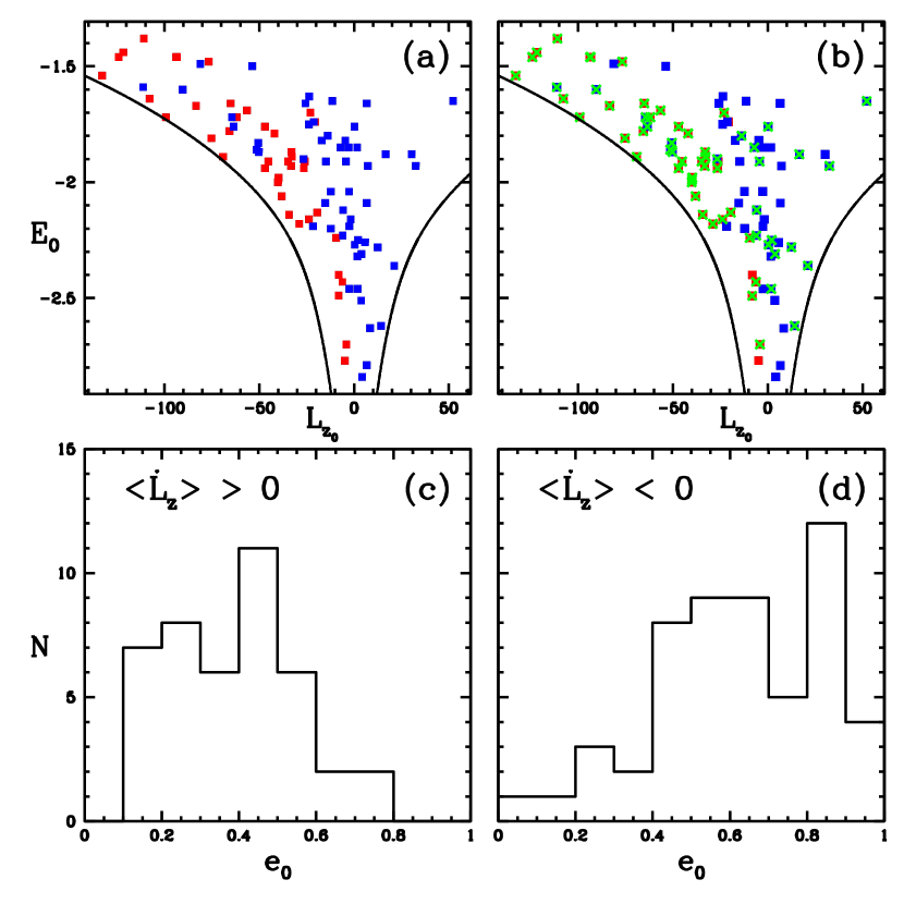
Figure 6: Distributions of clusters in the plane ($L_{z_{0}}$,$E_{0}$) and with respect to initial orbital eccentricity. In panel (a) the points with red colour correspond to clusters with positive $<\!\dot{L}_{z}\!>$, and those in blue colour, to clusters with negative $<\!\dot{L}_{z}\!>$. All the clusters with retrograde motion, i.e. $L_{z_{0}}$ > 0, have negative $<\!\dot{L}_{z}\!>$. Clusters with prograde motion, i.e. $L_{z_{0}}$ < 0, can have $<\!\dot{L}_{z}\!>$ positive or negative. The black curves represent prograde and retrograde circular orbits in the axisymmetric Galactic potential. In panel (b), the points marked with a green cross correspond to clusters that have an initial eccentricity, $e_{0}$, smaller than 0.6. Panels (c) and (d) show the details of the distributions in eccentricity for clusters with $<\!\dot{L}_{z}\!>$ positive and negative, i.e. red and blue points in panel (a).

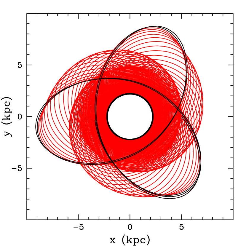
Figure 7: Orbit on the Galactic plane of a model cluster with a mass of $5\times 10^{5}M_{\sun}$ and $r_{h}$=10 pc. The orbit is initially extended and it becomes nearly circular at around 15 Gyr as shown in black.

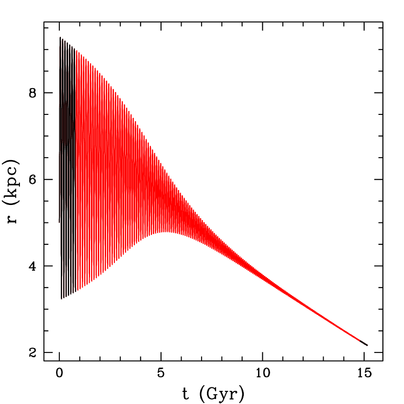
Figure 8: The variation of $r$ with time in the orbit shown in Fig. 7. The initial and final integration times are shown in black.

4.2 Local variations

In Section 4.1 we computed by means of linear least-square fits the mean variations $<\dot{E}>$, $<\!\dot{L}_{z}\!>$ over the first Gyr. Figs. 1–5 show smooth variations of $E$ and $L_{z}$. However, locally, around a given time, $\frac{{\rm d}E}{{\rm d}t}$ and $\frac{{\rm d}L_{z}}{{\rm d}t}$ can be positive and negative, as indicated for example in the curves $L_{z}$ vs t of NGC 6171 in Fig. 1 and NGC 6441 in Fig. 3. To illustrate the possible behaviour of $E$, $L_{z}$, $\frac{{\rm d}E}{{\rm d}t}$, and $\frac{{\rm d}L_{z}}{{\rm d}t}$, Figs. 9 and 10 show their dependence on time in Liller 1 and NGC 6749, in a short time interval at the beginning of the orbital computation. Panels (a) and (b) in both figures show $E$ vs t and $L_{z}$ vs t. The details in these curves can not be seen in the corresponding Figs. 2 and 5, which cover the total 5 Gyr interval. In Liller 1, $E$ and $L_{z}$ decline smoothly, but have maxima and minima in NGC 6749. Panels (c) and (d) in both figures give $\frac{{\rm d}E}{{\rm d}t}$ vs t, $\frac{{\rm d}L_{z}}{{\rm d}t}$ vs t, (magenta colour), along with the function $\frac{1}{r}$ (blue colour), multiplied by a convenient factor, to highlight the successive $r_{\rm min}$, $r_{\rm max}$ positions. The vertical dotted lines extended to panels (a),(b) localise two positions, one with $r_{\rm min}$ and the other with $r_{\rm max}$. In both clusters, panels (c) show that $|\frac{{\rm d}E}{{\rm d}t}|_{\rm max}$ occurs at perigalactic distance $r_{\rm min}$. The minimum value of $|\frac{{\rm d}E}{{\rm d}t}|$ is obtained at $r_{\rm max}$ in Liller 1, but in NGC 6749 $\frac{{\rm d}E}{{\rm d}t}$ can be positive around this apogalactic distance, with a value comparable with the magnitude of the variation reached at $r_{\rm min}$. The horizontal discontinuous lines in panels (c) show the mean time-variations $<\dot{E}>$ for these two clusters listed in Table 5. In both clusters, panels (d) show that $|\frac{{\rm d}L_{z}}{{\rm d}t}|_{\rm max}$ occurs at apogalactic distance $r_{\rm max}$, and $|\frac{{\rm d}L_{z}}{{\rm d}t}|_{\rm min}$ at $r_{\rm min}$; in NGC 6749 $\frac{{\rm d}L_{z}}{{\rm d}t}$ can change sign at this perigalactic distance. Also in these panels (d), the horizontal discontinuous lines give the mean time-variations $<\!\dot{L}_{z}\!>$ listed in Table 5.

The results shown in Figs. 9 and 10 can be explained as follows: Liller 1 has a retrograde motion (see Table 5), thus it is slowed down along its orbit due to the prograde motion of the background, and $\frac{{\rm d}E}{{\rm d}t}$, $\frac{{\rm d}L_{z}}{{\rm d}t}$ are always negative. $|\frac{{\rm d}E}{{\rm d}t}|$ is maximum at $r_{\rm min}$ due to the increase in density towards the Galactic Centre. $|\frac{{\rm d}L_{z}}{{\rm d}t}|$ is maximum at $r_{\rm max}$ because there the cluster has a slow motion and the background is moving fast in the opposite direction. At $r_{\rm min}$ the cluster is moving faster, but the background coming in the opposite direction has a slow motion, resulting in less deceleration. In NGC 6749, with a prograde motion (see Table 5), at $r_{\rm min}$ the cluster is moving faster than the background moving in the same direction, thus it is slowed down, it has less rotation and then $\frac{{\rm d}E}{{\rm d}t}$ is negative and $\frac{{\rm d}L_{z}}{{\rm d}t}$ positive. At $r_{\rm max}$, the cluster is moving slower than the background coming in the same direction, and it is accelerated, thus $\frac{{\rm d}E}{{\rm d}t}$ is positive and $|L_{z}|$ increases.

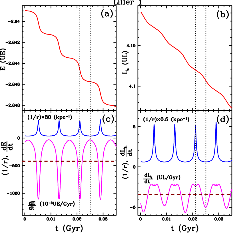
Figure 9: Local variations of $E$, $L_{z}$, $\frac{{\rm d}E}{{\rm d}t}$, $\frac{{\rm d}L_{z}}{{\rm d}t}$ in Liller 1 close to the beginning of its orbital computation. The units are those given in Table 5. Panels (a) and (b) show the smooth variations $E$ vs t and $L_{z}$ vs t. Panels (c) and (d) give $\frac{{\rm d}E}{{\rm d}t}$ vs t, $\frac{{\rm d}L_{z}}{{\rm d}t}$ vs t, (magenta colour), along with the function $\frac{1}{r}$ (blue colour), multiplied by a convenient factor, to highlight the successive $r_{\rm min}$, $r_{\rm max}$ positions. The vertical dotted lines extended to panels (a), (b) localise two positions, one with $r_{\rm min}$ and the other with $r_{\rm max}$. Panel (c) shows that $|\frac{{\rm d}E}{{\rm d}t}|_{\rm max}$ occurs at perigalactic distance $r_{\rm min}$. The minimum value of $|\frac{{\rm d}E}{{\rm d}t}|$ is obtained at $r_{\rm max}$. The horizontal dashed line shows the mean time-variation $<\dot{E}>$ for this cluster listed in Table 5. Panel (d) shows that $|\frac{{\rm d}L_{z}}{{\rm d}t}|_{\rm max}$ occurs at apogalactic distance $r_{\rm max}$, and $|\frac{{\rm d}L_{z}}{{\rm d}t}|_{\rm min}$ at $r_{\rm min}$. The horizontal dashed line gives the mean time-variation $<\!\dot{L}_{z}\!>$ listed in Table 5.

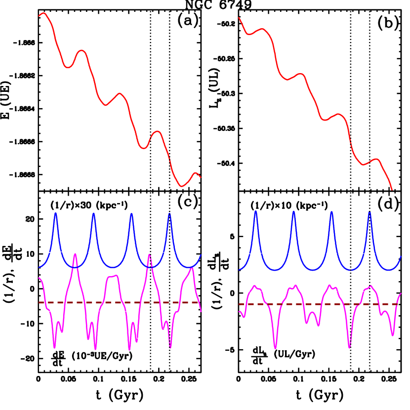
Figure 10: As in Fig. 9, here for NGC 6749. In this cluster, $E$ and $L_{z}$ present maxima and minima. Here $\frac{{\rm d}E}{{\rm d}t}$ can be positive around $r_{\rm max}$ with a value comparable with its maximum magnitude reached at $r_{\rm min}$, and $\frac{{\rm d}L_{z}}{{\rm d}t}$ can change sign at this perigalactic distance.

5 Some implications for the system of globular clusters

The globular cluster orbits of Figs. 1-5 show a wide range of effects due to dynamical friction, ranging from slight to moderate and up to extreme, such as for Liller 1, Terzan 4, Terzan 5, and NGC6440 where the orbits are seen to collapse both vertically as well as radially. These extreme cases may lead to very interesting results for analyses of the globular-cluster system and for Galactic evolution, such as the misclassification of the globulars between the categories ‘halo’, ‘bulge’, and ‘thick disc’ (Pérez-Villegas et al., 2020), the resulting biasing of globular-cluster samples, the incorrect association of the globulars with their parent dwarf galaxies for accretion events, and the possible formation of nuclear star clusters.

Globular clusters which had been part of the Galactic halo, with low metallicities and early formation in the Galaxy might now, due to dynamical friction, appear as members of the Galactic thick disc or bulge due to their new positions, velocities, and/or distributions in the Galaxy, as clearly appreciated for Liller 1, Terzan 4, Terzan 5, and NGC6440. These might very well be misclassified, and so samples of globular clusters for studying these components of the Galaxy: thick-disc, bulge, and halo, will be contaminated and biased. For example, globulars formed with the ages and metallicities of the halo might now be included, due to dynamical friction, in samples for the thick disc or bulge, biasing results for age and metallicity gradients, as well as for other characteristics, for the bulge, thick disc, and halo. The former two components will have some members with too low metallicities and perhaps too high ages, while the halo sample will be lacking some members.

For accreted globular clusters, the finer details of the hierarchical galaxy formation could be affected, such as not being able to separate cleanly their origin. Several studies have associated an accreted or formed-in-situ origin of some globular clusters (Bellazzini et al., 2003; Zolotov et al., 2009; Forbes & Bridges, 2010; Zolotov et al., 2010; Nissen & Schuster, 2010; Schuster et al., 2012; Myeong et al., 2018b; Helmi et al., 2018; Myeong et al., 2019; Massari et al., 2019; Koppelman et al., 2019; Forbes, 2020), but due to the not considerd effect of dynamical friction, this association might be uncertain. Regarding this issue, in the literature it has been usually assumed that in a cluster orbital evolution the orbital energy and $z$-component of angular momentum are constants, or vary slightly in time. This approximation has been employed to associate an accretion event with a possible accreted cluster. With the results listed in Tables 5 and 6, obtained under the effect of dynamical friction, we can estimate if this assumption is convenient. For all the clusters in both tables, Fig 11 shows the relative variations $<\Delta E>/E_{0}$, $<\!\Delta L_{z}\!>/L_{z_{0}}$. Liller 1 is not plotted in this figure since it is off scale, i.e. outside the vertical limits. Black open squares give the current variations, obtained over the first Gyr of the orbital computations, as obtained directly from the tables; in energy they are approximately smaller than 4 per cent, and in angular momentum the majority of clusters have variations smaller than 10 per cent. The red points in the figure are the corresponding relative variations extending the current values over a time interval of 10 Gyr. In this extension, in the majority of clusters the variation in energy is within 10 per cent, but in angular momentum it can reach about 50 per cent, or more, in some of them.

The extension to 10 Gyr gives an estimate of expected cluster orbital variations in energy and angular momentum over the lifetime of our Galaxy, applied to possible accreted globular clusters, and those formed in situ as well. In this extension, the clusters with relative variations in energy greater than 10 per cent are: Terzan 2, Terzan 4, Terzan 5, Liller 1, and NGC 6440. With relative variations in angular momentum greater than 10 per cent: NGC 5139, NGC 6093, NGC 6266, NGC 6273, NGC 6380, NGC 6388, NGC 6401, NGC 6440, NGC 6453, NGC 6522, NGC 6553, NGC 6624, NGC 6638, NGC 6642, NGC 6681, NGC 6712, NGC 6749, Terzan 1, Terzan 2, Terzan 4, Terzan 5, Terzan 6, Liller 1, Djorg 2, Pal 6, VVV-CL001, HP 1.

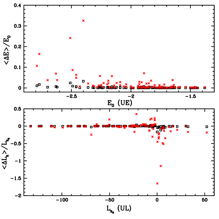
Figure 11: Relative variations in energy and angular momentum of clusters in Tables 5 and 6, except Liller 1. Black open squares show the current variations, over the first Gyr of the orbital computations. The red points show the variations extending the current values over an interval of 10 Gyr.

From these clusters with high variation in angular momentum, we separated in particular those with variations greater than 20 per cent. We computed their orbits backwards in time, i.e. in the past, up to 10 Gyr, with the effect of the dynamical friction and with the approximation of constant cluster mass, equal to the current mass. This underestimates the dynamical friction effect, as a cluster is more massive in the past. Also, as in all our computations, the change in time of the background Galactic potential is not considered. In Fig. 12 we show their meridional orbits in the first 0.5 Gyr of the computations, i.e. near the current time. Each panel shows the name of the cluster. Fig. 13 shows the orbits of these same clusters in the last 0.5 Gyr, i.e. from 9.5 Gyr to 10 Gyr in the past; the scale in each panel is the same as in Fig. 12, except in Liller 1. Table 7 lists the relative variations in energy and $z$-angular momentum in these clusters, during the total interval of 10 Gyr. In energy the variation in energy is less than 10 per cent, except in Liller 1. Only Terzan 2, HP 1, Liller 1, NGC 6380, NGC 6401, NGC 6440, and NGC 6681 present in angular momentum the estimated variation greater than 20 per cent. Thus, for the majority of computed clusters the approximation of nearly invariant energy and $z$- angular momentum seems appropriate.

Table 7: Relative variations in energy and angular momentum for the clusters in Figs. 12 and 13, during 10 Gyr backwards in time with the effect of dynamical friction.

Cluster	$<\!\Delta E\!>/E_{0}$	$<\!\Delta L_{z}\!>/L_{z_{0}}$
Terzan 2	$-$0.040	0.225
Terzan 4	$-$0.056	0.051
HP 1	$-$0.006	0.223
Liller 1	$-$0.150	2.126
NGC 6380	$-$0.024	0.326
Terzan 1	$-$0.016	$-$0.175
NGC 6401	$-$0.024	0.317
Pal 6	$-$0.009	0.139
NGC 6440	$-$0.067	0.718
Terzan 6	$-$0.028	0.157
NGC 6453	$-$0.009	$-$0.050
NGC 6553	$-$0.029	0.070
NGC 6624	$-$0.026	$-$0.144
NGC 6642	$-$0.005	0.084
NGC 6681	$-$0.003	0.712
NGC 6712	$-$0.003	0.137

Figs. 12 and 13 show that Terzan 2, Terzan 4, Terzan 6, NGC 6624, NGC 6642, HP 1, which have been classified as formed in situ in the Galactic bulge (see Tables 5 and 6), approximately maintain this classification over the 10 Gyr computed time. This appears only approximate in Terzan 1, NGC 6440, NGC 6380, Pal 6, with the same classification. However, NGC 6553 appears to come from a region external to the Galactic bulge, i.e. not formed in situ within this bulge. Liller 1 shows the strongest variation, and it needs a particular analysis. NGC 6401, NGC 6453, NGC 6681, NGC 6712, are associated with the $Koala$ dwarf galaxy accretion event (Forbes, 2020), and their orbits do not change strongly during 10 Gyr, in spite of the strong variation in angular momentum in NGC 6401 and NGC 6681. The results shown in Figs. 12 and 13 are preliminary, as we have assumed a constant cluster mass. A study varying the mass of clusters, similar to that presented by Baumgardt et al. (2019), could improve the comparison.

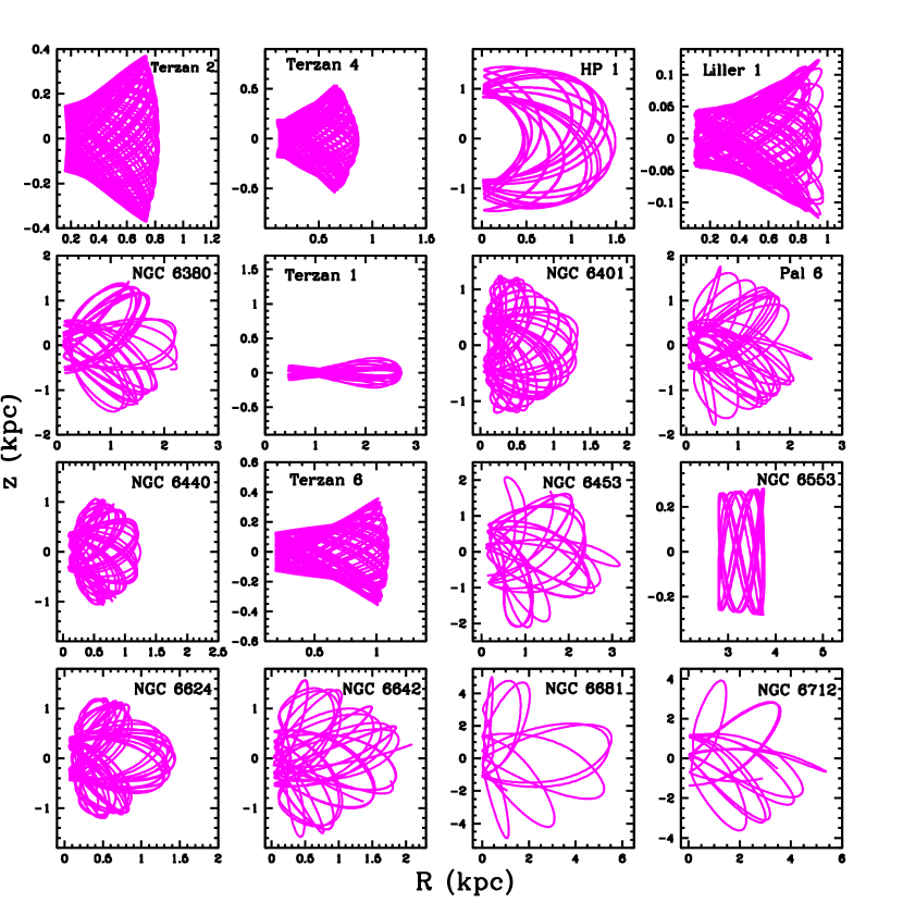
Figure 12: Meridional orbits of clusters with variations in angular momentum greater than 20 per cent, in the extension to 10 Gyr. The orbits are computed backwards in time up to 10 Gyr, and the figure shows the orbits in the first 0.5 Gyr, i.e. near the current time. The name of the cluster is shown in each panel.

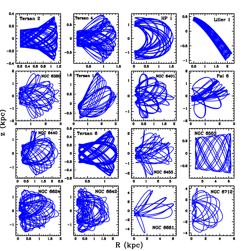
Figure 13: Meridional orbits of the clusters in Fig. 12, here shown in the time interval from 9.5 Gyr to 10 Gyr in the past. Notice the same scale in the panels as in Fig. 12, except in Liller 1.

Another process where globular clusters extremely affected by dynamical friction might be pertinent for understanding Galactic observations, would be globulars infalling toward the inner-most region of the Galaxy, and in many other galaxies as well, due to their rapidly collapsing orbits. This process could form nuclear star clusters (NSCs) (Tremaine et al., 1975; Capuzzo-Dolcetta, 1993; Oh & Lin, 2000; Lotz et al., 2001; Agarwal & Milosavljević, 2011; Capuzzo-Dolcetta, 2013; Antonini et al., 2012; Perets & Mastrobuono-Battisti, 2014; Gnedin et al., 2014; Schödel et al., 2014; Arca-Sedda et al., 2015; Tsatsi et al., 2017; Neumayer et al., 2020) and distributions of clusters around the nuclear galactic regions. Some massive accreted clusters in the Galaxy are themselves NSCs of accreted dwarf galaxies (Pfeffer et al., 2021). These infalling clusters might induce new star formation in the material near the central black hole, showing both very young as well as very old stars, as observed.

6 Conclusions

We have made a preliminary analysis of the effect of dynamical friction on some orbits of globular clusters in our Galaxy, considering an anisotropic velocity dispersion field approximated with some studies in the literature. An axisymmetric Galactic model with mass components disc, bulge, and dark halo is employed in the computations. We describe a procedure to compute the dynamical friction acceleration in ellipsoidal, oblate, and prolate velocity distribution functions with similar density in velocity space. Orbital properties, such as mean time-variations of perigalactic and apogalactic distances, energy, and z-component of angular momentum, are obtained for globular clusters lying in the Galactic region $R\lesssim$ 10 kpc, $|z|\lesssim$ 5 kpc, with $R,z$ cylindrical coordinates. These include clusters in prograde and retrograde orbital motion. Several clusters are strongly affected by dynamical friction, in particular, Liller 1, Terzan 4, Terzan 5, NGC 6440, and NGC 6553, lying in the Galactic inner region. Improvements to our computations can be made analysing with more detail the dispersion fields of the Galactic mass components, specially the thin and thick disc components. Introducing the properties of the dark halo outside galactocentric distance of 10 kpc will permit the analysis of the orbits of globular clusters not included in the present study. More extended analyses including these improvements will be presented in the future, using the detailed Galactic model GravPot16 (see footnote 1 in Section 3.4), considering the computation of tidal radii, destruction rates, and other properties of globular clusters related with the effect of dynamical friction.

We have pointed out some aspects in the analysis of the system of Galactic globular clusters which are directly related with the effect of dynamical friction. These include the possible misclassification of the globulars between the categories ‘halo’, ‘bulge’, and ‘thick disc’, the resulting biasing of globular-cluster samples, the possible incorrect association of the globulars with their parent dwarf galaxies for accretion events, and the possible formation of ‘nuclear star clusters’.

Data Availability

Data available on request.

Appendix A Force field of an ellipsoidal shell in velocity space with linear similar density

As in any continuous function, a density function $f_{0}$ in velocity space whose isodensity surfaces are similar ellipsoids, as in the case of $f_{0}$($r$,$v$) in Eq. 4, can be approximated by a series of connected linear segments, which are linear functions of an appropriate variable identifying the ellipsoidal surfaces. Thus, each linear segment represents a shell in velocity space, and the original density function can be reasonably approximated by taking a sufficiently large number of these shells. The total potential ${\Psi}$($r$,$v$_M) (see Eq. 5) and force field $-{\nabla}$${}_{\tiny v_{\rm M}}$${\Psi}$($r$,$v$_M) at point $v$_M are obtained with the sum of the individual fields of each shell.

We denote the semiaxes of an ellipsoidal surface in velocity space with the usual notation in ordinary space: $a,b,c$, along the Cartesian axes $({v}_{1},{v}_{2},{v}_{3})$, respectively, with $a$>$b$>$c$. The unitary vectors along the axes are ($e$₁,$e$₂,$e$₃). Taking the major semi-axis $a$ as the velocity variable which identifies the similar ellipsoidal surfaces, the linear density in a given shell with $a$ $\epsilon[a_{1},a_{2}]$ has the form $f_{0}(a)=p_{0}+p_{1}a$, with $p_{0},p_{1}$ constants which are obtained in terms of $f_{0}$ evaluated at $a_{1},a_{2}$. With $a=ma_{2}$, $m$ $\epsilon[m_{1},1],a_{1}=m_{1}a_{2}$, the density in the shell is $f_{0}[m]=p_{0}+p_{1}a_{2}m$, and its potential at any point $v$=$({v}_{1},{v}_{2},{v}_{3})$ can be obtained with potential theory (e.g., Kellogg, 1953). The given point $v$ lies on a similar ellipsoidal surface with major semi-axis denoted by $a$($v$) in the following analysis.

(a) $v$ external to the shell, i.e. $a$($v$)$\geq a_{2}$.

In the region external to the shell, i.e. $a$($v$)$\geq a_{2}$, the potential is (in the following we omit in the potential its dependence on $r$)

$${\Psi}(\mbox{\boldmath$v$})=-2\pi a_{2}^{3}\zeta\xi\int_{m_{1}}^{1}f_{0}[m]m^{2}{\rm d}m\int_{\lambda(m)}^{\infty}\frac{{\rm d}s}{\sqrt{\varphi(m,s)}},$$ (25)

where the function $\varphi(m,s)$ is given by

$$\varphi(m,s)=(m^{2}a_{2}^{2}+s)(m^{2}\zeta^{2}a_{2}^{2}+s)(m^{2}\xi^{2}a_{2}^{2}+s),$$ (26)

the factors $\zeta=b/a$, $\xi=c/a$ are constant ratios in the similar ellipsoids, and $\lambda(m)$ is the greatest root of $s$ in the cubic equation resulting from

$$\frac{{v}_{1}^{2}}{m^{2}a_{2}^{2}+s}+\frac{{v}_{2}^{2}}{m^{2}\zeta^{2}a_{2}^{2}+s}+\frac{{v}_{3}^{2}}{m^{2}\xi^{2}a_{2}^{2}+s}-1=0.$$ (27)

Introducing $f_{0}[m]=p_{0}+p_{1}a_{2}m$ in Eq. (25), with the change of variable $s=m^{2}t$ in the inner integral, and integrating by parts, we obtain

$${\Psi}(\mbox{\boldmath$v$}) = {\Psi}_{p_{0}}(\mbox{\boldmath$v$})+{\Psi}_{p_{1}}(\mbox{\boldmath$v$})=-\pi p_{0}a_{2}^{3}\zeta\xi(I_{1}-m_{1}^{2}I_{2}+I_{3})-$$ (28)

$$-\frac{2}{3}\pi p_{1}a_{2}^{4}\zeta\xi(I_{1}-m_{1}^{3}I_{2}+I_{4}),$$

with

$$I_{1}=\int_{\lambda}^{\infty}\frac{{\rm d}t}{\sqrt{\varphi(t)}},~{}~{}~{}~{}~{}I_{2}=\int_{u(m_{1})}^{\infty}\frac{{\rm d}t}{\sqrt{\varphi(t)}},$$ (29)

$$I_{3}=\int_{u(m_{1})}^{\lambda}\frac{m^{2}(u){\rm d}u}{\sqrt{\varphi(u)}},~{}~{}~{}~{}~{}I_{4}=\int_{u(m_{1})}^{\lambda}\frac{m^{3}(u){\rm d}u}{\sqrt{\varphi(u)}},$$ (30)

$$\varphi(t)=(a_{2}^{2}+t)(\zeta^{2}a_{2}^{2}+t)(\xi^{2}a_{2}^{2}+t),$$ (31)

$$m(u)=\left[\frac{{v}_{1}^{2}}{a_{2}^{2}+u}+\frac{{v}_{2}^{2}}{\zeta^{2}a_{2}^{2}+u}+\frac{{v}_{3}^{2}}{\xi^{2}a_{2}^{2}+u}\right]^{1/2},$$ (32)

and $u(m_{1})=\lambda(m_{1})/m_{1}^{2}$, $\lambda=\lambda(m=1)$. Now, with

$$\sin\phi_{1} =a_{2}\left[\frac{1-\xi^{2}}{a_{2}^{2}+u(m_{1})}\right]^{1/2},$$ (33)

$$\sin\phi_{2} =a_{2}\left[\frac{1-\xi^{2}}{a_{2}^{2}+\lambda}\right]^{1/2},$$ (34)

$$k =\left[\frac{1-\zeta^{2}}{1-\xi^{2}}\right]^{1/2},$$ (35)

the integrals $I_{1}$, $I_{2}$ are

$$I_{1}=\frac{2F(k,\phi_{2})}{a_{2}\sqrt{1-\xi^{2}}},~{}~{}~{}I_{2}=\frac{2F(k,\phi_{1})}{a_{2}\sqrt{1-\xi^{2}}},$$ (36)

with $F(k,\phi)$ being the Legendre elliptic integral of the 1st kind.

Introducing Eq. (32) in the integrand of $I_{3}$, this integral $I_{3}$ is a combination of the following three integrals, where we use expressions in (33), (34), (35), with $k^{\prime}=\sqrt{1-k^{2}}$, and $E(k,\phi)$ being the Legendre elliptic integral of the 2nd kind

$$I_{5} = \int_{u(m_{1})}^{\lambda}\frac{{\rm d}u}{(a_{2}^{2}+u)\sqrt{\varphi(u)}}=\frac{2}{a_{2}^{3}(1-\xi^{2})^{3/2}k^{2}}\left[F(k,\phi_{1})-\right.$$ (37)

$$\left.-F(k,\phi_{2})-[E(k,\phi_{1})-E(k,\phi_{2})]\right],$$

$$I_{6} = \int_{u(m_{1})}^{\lambda}\frac{{\rm d}u}{(\zeta^{2}a_{2}^{2}+u)\sqrt{\varphi(u)}}=$$ (39)

$$= \frac{2}{a_{2}^{3}(1-\xi^{2})^{3/2}k^{2}k^{\prime 2}}\left.\bigg{\{}k^{\prime 2}[F(k,\phi_{2})-F(k,\phi_{1})]-\right.$$

$$\left.-k^{2}\left[\frac{\sin\phi_{1}\cos\phi_{1}}{\sqrt{1-k^{2}\sin^{2}\phi_{1}}}-\frac{\sin\phi_{2}\cos\phi_{2}}{\sqrt{1-k^{2}\sin^{2}\phi_{2}}}\right]+\right.$$

$$\left.+E(k,\phi_{1})-E(k,\phi_{2})\right.\bigg{\}},$$

$$I_{7} = \int_{u(m_{1})}^{\lambda}\frac{{\rm d}u}{(\xi^{2}a_{2}^{2}+u)\sqrt{\varphi(u)}}=$$ (41)

$$= \frac{2}{a_{2}^{3}(1-\xi^{2})^{3/2}k^{\prime 2}}\left[\sqrt{1-k^{2}\sin^{2}\phi_{1}}\tan\phi_{1}-\right.$$

$$-\sqrt{1-k^{2}\sin^{2}\phi_{2}}\tan\phi_{2}-$$

$$-[E(k,\phi_{1})-E(k,\phi_{2})]\Bigg{]}.$$

One way to solve the remaining integral $I_{4}$ is to note that from expressions (31) and (32), $m(u)\sqrt{\varphi(u)}$ can be written as

$$m(u)\sqrt{\varphi(u)}=(Au^{2}+Bu+C)^{1/2},$$ (42)

with $A,B,C$ functions of $({v}_{1},{v}_{2},{v}_{3})$. Thus, writing the integrand in $I_{4}$ as $m^{4}(u)/(Au^{2}+Bu+C)^{1/2}$, $I_{4}$ can be obtained as the sum of six integrals easily computed with standard tables (e.g., Gradshteyn & Ryzhik, 2000). This completes the computation of the potential in Eq. (28).

The force field is obtained with the negative gradient of the potential. For the part ${\Psi}_{p_{0}}$($v$) in Eq. (28) we have

$$-\frac{\partial{\Psi}_{p_{0}}}{\partial{v}_{1}} = \pi p_{0}a_{2}^{3}\zeta\xi\left[-\frac{1}{\sqrt{\varphi(\lambda)}}\frac{\partial\lambda}{\partial{v}_{1}}+\frac{m_{1}^{2}}{\sqrt{\varphi(u(m_{1}))}}\frac{\partial u(m_{1})}{\partial{v}_{1}}+\right.$$ (43)

$$+\int_{u(m_{1})}^{\lambda}\frac{\partial m^{2}(u)}{\partial{v}_{1}}\frac{{\rm d}u}{\sqrt{\varphi(u)}}+\frac{m^{2}(\lambda)}{\sqrt{\varphi(\lambda)}}\frac{\partial\lambda}{\partial{v}_{1}}-$$

$$\left.-\frac{m^{2}(u(m_{1}))}{\sqrt{\varphi(u(m_{1}))}}\frac{\partial u(m_{1})}{\partial{v}_{1}}\right].$$

The sum of the first and fourth terms inside the parenthesis in this last equation is zero, because from Eqs. (27) and (32) $\lambda$ is a root of $m^{2}(u)-1=0$. Also, the sum of the second and last terms is zero; this sum has the factor

$$m_{1}^{2}-m^{2}(u(m_{1})) = m_{1}^{2}\left[1-\frac{{v}_{1}^{2}}{a_{1}^{2}+\lambda(m_{1})}-\frac{{v}_{2}^{2}}{\zeta^{2}a_{1}^{2}+\lambda(m_{1})}-\right.$$ (44)

$$\left.-\frac{{v}_{3}^{2}}{\xi^{2}a_{1}^{2}+\lambda(m_{1})}\right],$$

and with Eq. (27) $\lambda(m_{1})$ cancels the expression inside the parenthesis. Thus, with expressions (32) and (37)

$$-\frac{\partial{\Psi}_{p_{0}}}{\partial{v}_{1}}=2\pi p_{0}a_{2}^{3}\zeta\xi{v}_{1}I_{5}.$$ (45)

Analogously

$$-\frac{\partial{\Psi}_{p_{0}}}{\partial{v}_{2}}=2\pi p_{0}a_{2}^{3}\zeta\xi{v}_{2}I_{6},$$ (46)

$$-\frac{\partial{\Psi}_{p_{0}}}{\partial{v}_{3}}=2\pi p_{0}a_{2}^{3}\zeta\xi{v}_{3}I_{7}.$$ (47)

Proceeding in a similar way with the term ${\Psi}_{p_{1}}$($v$) in Eq. (28), we obtain

$$-\frac{\partial{\Psi}_{p_{1}}}{\partial{v}_{1}}=2\pi p_{1}a_{2}^{4}\zeta\xi{v}_{1}\int_{u(m_{1})}^{\lambda}\frac{m^{2}(u){\rm d}u}{(a_{2}^{2}+u)\sqrt{Au^{2}+Bu+C}},$$ (48)

$$-\frac{\partial{\Psi}_{p_{1}}}{\partial{v}_{2}}=2\pi p_{1}a_{2}^{4}\zeta\xi{v}_{2}\int_{u(m_{1})}^{\lambda}\frac{m^{2}(u){\rm d}u}{(\zeta^{2}a_{2}^{2}+u)\sqrt{Au^{2}+Bu+C}},$$ (49)

$$-\frac{\partial{\Psi}_{p_{1}}}{\partial{v}_{3}}=2\pi p_{1}a_{2}^{4}\zeta\xi{v}_{3}\int_{u(m_{1})}^{\lambda}\frac{m^{2}(u){\rm d}u}{(\xi^{2}a_{2}^{2}+u)\sqrt{Au^{2}+Bu+C}}.$$ (50)

The three integrals resulting in each of the Eqs. (48), (49), (50), are also computed with standard tables. The total components of the force field due to the shell are given by adding Eq. (45) with Eq. (48), Eq. (46) with Eq. (49), and Eq. (47) with Eq. (50).

(b) $v$ inside the shell, i.e. $a$($v$) $\epsilon[a_{1},a_{2}]$.

In this case all the expressions obtained in part (a) are directly employed, but now instead of the limits of integration $\lambda$ these limits are changed to zero. If $a$($v$) = $a_{1}$, all the force components are zero.

(c) $v$ inside the cavity of the shell, i.e. $a$($v$)$<a_{1}$. The force components are zero.

Appendix B Force field of an oblate shell in velocity space with linear similar density

(a) $v$ external to the shell, i.e. $a$($v$)$\geq a_{2}$.

In the oblate system we take $a=b$, i.e. $\zeta=1$, and define $R=\sqrt{{v}_{1}^{2}+{v}_{2}^{2}}$, the eccentricity of the oblate shell $e_{\rm o}=\sqrt{1-\xi^{2}}$, and find the solutions $\beta_{1}$, $\beta_{2}$ of the equations

$$\begin{array}[]{rcl}R^{2}\sin^{2}\beta_{1}+{v}_{3}^{2}\tan^{2}\beta_{1}&=&a_{1}^{2}e_{\rm o}^{2},\\ R^{2}\sin^{2}\beta_{2}+{v}_{3}^{2}\tan^{2}\beta_{2}&=&a_{2}^{2}e_{\rm o}^{2}.\end{array}$$ (51)

As in Appendix A, the potential is expressed in the form $\Psi$($v$)= ${\Psi}_{p_{0}}$($v$)+ ${\Psi}_{p_{1}}$($v$). The Cartesian components of force corresponding to ${\Psi}_{p_{0}}$($v$) are

$$-\frac{\partial{\Psi}_{p_{0}}}{\partial{v}_{1}}=\frac{2\pi p_{0}\xi{v}_{1}}{e_{\rm o}^{3}}\left[F_{1}(\beta_{2})-F_{1}(\beta_{1})\right],$$ (52)

$$-\frac{\partial{\Psi}_{p_{0}}}{\partial{v}_{2}}=\frac{2\pi p_{0}\xi{v}_{2}}{e_{\rm o}^{3}}\left[F_{1}(\beta_{2})-F_{1}(\beta_{1})\right],$$ (53)

$$-\frac{\partial{\Psi}_{p_{0}}}{\partial{v}_{3}}=\frac{2\pi p_{0}\xi{v}_{3}}{e_{\rm o}^{3}}\left[F_{2}(\beta_{2})-F_{2}(\beta_{1})\right],$$ (54)

with the functions $F_{1}(\beta)$=$\sin\beta\cos\beta-\beta$, $F_{2}(\beta)$=$2(\beta-\tan\beta)$.

The corresponding Cartesian components of force for ${\Psi}_{p_{1}}$($v$) are

$$-\frac{\partial{\Psi}_{p_{1}}}{\partial{v}_{1}}=2\pi p_{1}\xi{v}_{1}\left[F_{3}(\beta_{2})-F_{3}(\beta_{1})\right],$$ (55)

$$-\frac{\partial{\Psi}_{p_{1}}}{\partial{v}_{2}}=2\pi p_{1}\xi{v}_{2}\left[F_{3}(\beta_{2})-F_{3}(\beta_{1})\right],$$ (56)

$$-\frac{\partial{\Psi}_{p_{1}}}{\partial{v}_{3}}=2\pi p_{1}\xi\left[F_{4}(\beta_{2})-F_{4}(\beta_{1})\right],$$ (57)

there is no external factor ${v}_{3}$ in Eq. (57) and the functions $F_{3},F_{4}$ are given by

$$\begin{array}[]{rcl}F_{3}(\beta)&=&\frac{1}{e_{\rm o}^{4}}(F_{5}(\beta)-F_{6}(\beta)),\\ F_{4}(\beta)&=&\frac{1}{e_{\rm o}^{4}}(-zF_{5}(\beta)+F_{7}(\beta)),\end{array}$$ (58)

with the functions $F_{5},F_{6},F_{7}$ being

$$F_{5}(\beta)=2\sqrt{R^{2}\cos^{2}\beta+{v}_{3}^{2}}+{v}_{3}\ln\frac{\sqrt{R^{2}\cos^{2}\beta+{v}_{3}^{2}}-{v}_{3}}{\sqrt{R^{2}\cos^{2}\beta+{v}_{3}^{2}}+{v}_{3}},$$ (59)

$$F_{6}(\beta)=\frac{2(R^{2}\cos^{2}\beta+{v}_{3}^{2})^{3/2}}{3R^{2}},$$ (60)

$$F_{7}(\beta)=-\frac{{v}_{3}\sqrt{R^{2}\cos^{2}\beta+{v}_{3}^{2}}}{\cos^{2}\beta}+\frac{1}{2}R^{2}\ln\frac{\sqrt{R^{2}\cos^{2}\beta+{v}_{3}^{2}}-{v}_{3}}{\sqrt{R^{2}\cos^{2}\beta+{v}_{3}^{2}}+{v}_{3}}.$$ (61)

The total components of the force field due to the shell are given by adding Eq. (52) with Eq. (55), Eq. (53) with Eq. (56), and Eq. (54) with Eq. (57).

(b) $v$ inside the shell, i.e. $a$($v$) $\epsilon[a_{1},a_{2}]$.

In this situation, $\beta_{2}$ is given by $\beta_{2}=\arcsin e_{\rm o}$. If $a$($v$)$>a_{1}$ and $a_{1}\neq 0$, $\beta_{1}$ is again the solution of the first equation in (51), with $\beta_{1}=0$ in the case $a_{1}=0$. All the expressions in part (a) are employed to compute the force field. If $a$($v$) = $a_{1}$, for any value of $a_{1}$ all the force components are zero.

(c) $v$ inside the cavity of the shell, i.e. $a$($v$)$<a_{1}$. The force components are zero.

Appendix C Force field of a prolate shell in velocity space with linear similar density

(a) $v$ external to the shell, i.e. $a$($v$)$\geq a_{2}$.

In this case we take $b=c$, and define $\mathcal{R}=\sqrt{{v}_{2}^{2}+{v}_{3}^{2}}$, the eccentricity of the prolate shell $e_{\rm p}=\sqrt{1-\xi^{2}}$, and find the solutions $\beta_{1}$, $\beta_{2}$ of the equations

$$\begin{array}[]{rcl}{v}_{1}^{2}\sin^{2}\beta_{1}+\mathcal{R}^{2}\tan^{2}\beta_{1}&=&a_{1}^{2}e_{\rm p}^{2},\\ {v}_{1}^{2}\sin^{2}\beta_{2}+\mathcal{R}^{2}\tan^{2}\beta_{2}&=&a_{2}^{2}e_{\rm p}^{2}.\end{array}$$ (62)

As in Appendix A, the potential is expressed in the form $\Psi$($v$)= ${\Psi}_{p_{0}}$($v$)+ ${\Psi}_{p_{1}}$($v$). The Cartesian components of force corresponding to ${\Psi}_{p_{0}}$($v$) are

$$-\frac{\partial{\Psi}_{p_{0}}}{\partial{v}_{1}}=\frac{2\pi p_{0}\xi^{2}{v}_{1}}{e_{\rm p}^{3}}\left[H_{1}(\beta_{2})-H_{1}(\beta_{1})\right],$$ (63)

$$-\frac{\partial{\Psi}_{p_{0}}}{\partial{v}_{2}}=\frac{2\pi p_{0}\xi^{2}{v}_{2}}{e_{\rm p}^{3}}\left[H_{2}(\beta_{2})-H_{2}(\beta_{1})\right],$$ (64)

$$-\frac{\partial{\Psi}_{p_{0}}}{\partial{v}_{3}}=\frac{2\pi p_{0}\xi^{2}{v}_{3}}{e_{\rm p}^{3}}\left[H_{2}(\beta_{2})-H_{2}(\beta_{1})\right],$$ (65)

with the functions $H_{1}(\beta)$=2$(\sin\beta-\ln[(1+\sin\beta)/\cos\beta])$, $H_{2}(\beta)$=$\ln[(1+\sin\beta)/\cos\beta]-\sin\beta/\cos^{2}\beta$.

The corresponding Cartesian components of force for ${\Psi}_{p_{1}}$($v$) are

$$-\frac{\partial{\Psi}_{p_{1}}}{\partial{v}_{1}}=\frac{2\pi p_{1}\xi^{2}H_{3}}{e_{\rm p}^{4}},$$ (66)

$$-\frac{\partial{\Psi}_{p_{1}}}{\partial{v}_{2}}=\frac{2\pi p_{1}\xi^{2}{v}_{2}H_{4}}{e_{\rm p}^{4}},$$ (67)

$$-\frac{\partial{\Psi}_{p_{1}}}{\partial{v}_{3}}=\frac{2\pi p_{1}\xi^{2}{v}_{3}H_{4}}{e_{\rm p}^{4}},$$ (68)

there is no factor ${v}_{1}$ in Eq. (66) and the functions $H_{3},H_{4}$ are given by

$$H_{3} = -{v}_{1}\left[(2+\cos^{2}\beta_{2})\frac{S_{2}^{1/2}}{\cos\beta_{2}}-(2+\cos^{2}\beta_{1})\frac{S_{1}^{1/2}}{\cos\beta_{1}}\right]\pm$$ (69)

$$\pm(\mathcal{R}^{2}-2{v}_{1}^{2})L,$$

with + sign if ${v}_{1}>0$ and $-$ sign if ${v}_{1}<0$,

$$H_{4} = -\frac{2}{3\mathcal{R}^{2}}\left[\frac{S_{2}^{3/2}}{\cos^{3}\beta_{2}}-\frac{S_{1}^{3/2}}{\cos^{3}\beta_{1}}\right]+2\left[\frac{S_{2}^{1/2}}{\cos\beta_{2}}-\frac{S_{1}^{1/2}}{\cos\beta_{1}}\right]+$$ (70)

$$+2|{v}_{1}|L,$$

with the functions

$$\begin{array}[]{rcl}S_{1}&=&{v}_{1}^{2}\cos^{2}\beta_{1}+\mathcal{R}^{2},\\ S_{2}&=&{v}_{1}^{2}\cos^{2}\beta_{2}+\mathcal{R}^{2},\\ L&=&\ln\frac{S_{2}^{1/2}-|{v}_{1}|\cos\beta_{2}}{S_{1}^{1/2}-|{v}_{1}|\cos\beta_{1}}.\end{array}$$ (71)

The total components of the force field due to the shell are given by adding Eq. (63) with Eq. (66), Eq. (64) with Eq. (67), and Eq. (65) with Eq. (68).

(b) $v$ inside the shell, i.e. $a$($v$) $\epsilon[a_{1},a_{2}]$.

In this situation, $\beta_{2}$ is given by $\beta_{2}=\arcsin e_{\rm p}$. If $a$($v$)$>a_{1}$ and $a_{1}\neq 0$, $\beta_{1}$ is again the solution of the first equation in (62), with $\beta_{1}=0$ in the case $a_{1}=0$. All the expressions in part (a) are employed to compute the force field. If $a$($v$) = $a_{1}$, for any value of $a_{1}$ all the force components are zero.

(c) $v$ inside the cavity of the shell, i.e. $a$($v$)$<a_{1}$. The force components are zero.

Appendix D Comparison of perigalactic and apogalactic distances in two Galactic models, without the dynamical friction effect

We compare here the mean perigalactic and apogalactic distances reached by some globular clusters, computed without the dynamical friction effect, as obtained with the Galactic model employed in this work, and with Galactic Model 2 used by Gaia Collaboration et al. (2018b) and in the Holger Baumgardt compilation cited in Section 4, which is the corresponding Model I of Irrgang et al. (2013). These two axisymmetric Galactic models which are employed in this comparison are slight modifications of the original model presented by Allen & Santillán (1991). Thus, under equal orbital initial conditions, no great differences are expected in the computations of Galactic orbits using these models. Table 8 shows the mean values of $<\!r_{\rm min}\!>$ and $<\!r_{\rm max}\!>$ in some clusters analysed in the present work, obtained with our model and with Irrgang’s model. Although both Galactic models and the orbital initial conditions (dependent on different assumed positions of the Sun and its peculiar velocity, motion of the local standard of rest, distances and radial velocities from the Sun, etc.) are not exactly the same in this work and in the analyses presented by Gaia Collaboration et al. (2018b) and Holger Baumgardt compilation, the corresponding listed values of the perigalactic and apogalactic distances compare well.

Table 8: Comparison in some clusters. Columns with label 1 give properties obtained with the Galactic model employed in this work, those with label 2 and 3 list respectively results from Gaia Collaboration et al. (2018b) and the Holger Baumgardt compilation, using the Galactic Model I of Irrgang et al. (2013).

	$<\!r_{\rm min}\!>$ (kpc)				$<\!r_{\rm max}\!>$ (kpc)
	1	2	3		1	2	3
NGC 104	5.76	5.68	5.47		7.45	7.68	7.51
NGC 4372	2.96	3.14	2.92		7.25	7.40	7.24
NGC 4833	0.97	0.93	0.85		7.24	7.86	7.65
NGC 5139	1.87	1.29	1.50		6.88	7.26	6.94
NGC 5927	4.24	4.31	4.03		5.67	5.19	5.46
NGC 5946	0.61	0.76	0.49		4.97	5.72	5.18
NGC 5986	0.62	0.52	0.56		5.24	4.95	5.05
NGC 6093	0.84	0.60	0.87		4.39	3.89	4.07
NGC 6121	0.90	0.41	0.68		5.97	6.08	6.44
NGC 6144	1.86	2.39	1.90		3.24	2.96	3.13
NGC 6171	0.89	0.94	1.22		4.38	3.74	3.83
NGC 6218	2.08	2.41	2.15		4.80	5.00	4.71
NGC 6235	3.46	3.15	3.49		8.57	5.04	7.47
NGC 6254	1.93	2.30	1.92		4.56	5.28	4.59
NGC 6266	0.85	0.69	0.86		2.33	2.36	2.42
NGC 6273	1.09	1.32	1.21		3.32	3.38	3.28
NGC 6284	0.89	1.07	0.99		6.56	7.31	6.43
NGC 6287	0.56	1.24	0.88		4.65	4.74	4.16
NGC 6293	0.47	0.47	0.47		2.74	2.81	2.74
NGC 6304	1.45	1.87	1.55		2.66	3.13	2.69
NGC 6316	1.09	0.42	0.90		3.89	2.59	3.92
NGC 6325	0.95	1.15	1.04		1.29	1.35	1.31
NGC 6333	0.91	1.45	1.22		7.07	3.52	6.16
NGC 6342	0.74	0.97	0.83		1.67	1.66	1.67
NGC 6352	3.11	3.20	3.08		4.11	4.36	3.93
NGC 6356	3.72	2.64	3.53		8.94	7.55	8.97
NGC 6362	2.80	5.12	2.65		5.22	6.83	5.24
NGC 6366	2.09	3.56	2.21		5.87	5.38	5.71
NGC 6380	0.33	0.39	0.30		2.02	2.90	2.10
NGC 6388	1.28	0.74	1.15		3.83	3.18	4.07
NGC 6397	2.41	2.90	2.61		6.28	6.59	6.30
NGC 6401	0.23	2.40	0.29		1.31	3.90	1.55
NGC 6402	0.62	0.51	0.53		4.24	4.32	4.28
NGC 6440	0.16	0.23	0.22		1.30	1.30	1.26
NGC 6441	1.65	0.80	1.59		4.72	3.43	4.71
NGC 6453	0.37	1.22	0.48		2.68	3.62	2.58
NGC 6496	2.45	3.79	2.62		5.33	8.11	4.62
NGC 6517	0.45	0.49	0.44		3.26	4.04	3.36
NGC 6522	0.20	0.31	0.45		1.41	1.23	1.31
NGC 6528	0.40	0.39	0.42		0.72	1.03	0.92
NGC 6535	1.18	1.10	0.97		4.31	4.52	4.52
NGC 6539	2.02	1.95	2.11		3.37	3.29	3.41
NGC 6541	1.59	1.44	1.56		3.62	3.70	3.59
NGC 6544	0.66	0.39	0.60		5.16	5.23	5.54
NGC 6626	0.47	0.58	0.59		3.05	3.15	3.03
NGC 6637	0.36	0.32	0.39		2.06	1.93	2.06
NGC 6656	3.04	3.21	2.96		9.82	9.92	9.59
NGC 6681	0.54	1.16	0.86		5.49	4.31	4.97
NGC 6752	3.49	3.64	3.37		5.62	5.72	5.48
NGC 6809	1.45	1.59	1.57		5.78	5.82	5.62
NGC 6838	4.86	4.99	4.81		7.08	7.30	7.12

References

- Allen & Santillán (1991) Allen C., Santillán A., 1991, Rev. Mex. Astron. Astrofis., 22, 255
- Agarwal & Milosavljević (2011) Agarwal M., Milosavljević M., 2011, ApJ, 729, 35
- Antonini et al. (2012) Antonini F., Capuzzo-Dolcetta R., Mastrobuono-Battisti A., Merritt D., 2012, ApJ, 750, 111
- Arca-Sedda et al. (2015) Arca-Sedda M., Capuzzo-Dolcetta R., Antonini F., Seth A., 2015, ApJ, 806, 220
- Battaglia et al. (2005) Battaglia G., Helmi A., Morrison H., et al., 2005, MNRAS, 364, 433
- Battaglia et al. (2006) Battaglia G., Helmi A., Morrison H., et al., 2006, MNRAS, 370, 1055
- Baumgardt et al. (2019) Baumgardt H., Hilker M., Sollima A., Bellini A., 2019, MNRAS, 482, 5138
- Beaulieu et al. (2000) Beaulieu S. F., Freeman K. C., Kalnajs A. J., Saha P., Zhao H. S., 2000, AJ, 120, 855
- Belokurov et al. (2018) Belokurov V., Erkal D., Evans N. W., Koposov S. E., Deason A. J., 2018, MNRAS, 478, 611
- Bellazzini et al. (2003) Bellazzini M., Ferraro F. R., Ibata R., 2003, AJ, 125, 188
- Binney & Tremaine (2008) Binney J., Tremaine S., 2008, Galactic Dynamics, 2nd ed., Princeton Univ. Press, Princeton
- Bird et al. (2019) Bird S. A., Xue X.-X., Liu C., Shen J., Flynn C., Yang C., 2019, AJ, 157, 104
- Bond et al. (2010) Bond N. A., Ivezić Ž., Sesar, B., et al., 2010, ApJ, 716, 1
- Brandt (1960) Brandt J. C., 1960, ApJ, 131, 293
- Brown et al. (2010) Brown W. R., Geller M. J., Kenyon S. J., Diaferio A., 2010, AJ, 139, 59
- Capuzzo-Dolcetta (1993) Capuzzo-Dolcetta R., 1993, ApJ, 415, 616
- Capuzzo-Dolcetta (2013) Capuzzo-Dolcetta R., 2013, Mem. Soc. Astron. Italiana, 84, 167
- Carollo et al. (2010) Carollo D., Beers T. C., Chiba M., et al., 2010, ApJ, 712, 692
- Casertano et al. (1987) Casertano S., Phinney E. S., Villumsen J. V., 1987, IAU Symp., 127, 475
- Chandrasekhar (1943) Chandrasekhar S., 1943, ApJ, 97, 255
- Chiba & Beers (2000) Chiba M., Beers T. C., 2000, AJ, 119, 2843
- Deason et al. (2017) Deason A. J., Belokurov V., Koposov S. E., Gómez F. A., Grand R. J., Marinacci F., Pakmor R., 2017, MNRAS, 470, 1259
- Dehnen et al. (2006) Dehnen W., McLaughlin D. E., Sachania J., 2006, MNRAS, 369, 1688
- Du et al. (2020) Du H., Mao S., Athanassoula E., Shen J., Pietrukowicz P., 2020, MNRAS, 498, 5629
- Fehlberg (1968) Fehlberg E., 1968, in NASA Technical Report R-287, Classical Fifth-, Sixth-, Seventh-, and Eighth-Order Runge-Kutta Formulas with Stepsize Control (Washington, DC: NASA)
- Fermani & Schönrich (2013) Fermani F., Schönrich R., 2013, MNRAS, 432, 2402
- Fernández-Trincado et al. (2016) Fernández-Trincado J. G., Robin A. C., Moreno E., et al., 2016, ApJ, 833, 132
- Fernández-Trincado (2017a) Fernández-Trincado J. G., 2017a, PhD Thesis, University Bourgogne Franche-Comté, France
- Fernández-Trincado et al. (2017b) Fernández-Trincado J. G., Zamora O., García-Hernández D. A., et al., 2017b, ApJ, 846, L2
- Fernández-Trincado et al. (2019a) Fernández-Trincado J. G., Beers T. C., Tang B., Moreno E., Pérez-Villegas A., Ortigoza-Urdaneta M., 2019a, MNRAS, 488, 2864
- Fernández-Trincado et al. (2019b) Fernández-Trincado J. G., Beers T. C., Placco V. M., et al., 2019b, ApJ, 886, L8
- Fernández-Trincado et al. (2020a) Fernández-Trincado J. G., Chaves-Velasquez L., Pérez-Villegas A., Vieira K., Moreno E., Ortigoza-Urdaneta M., Vega-Neme L., 2020a, MNRAS, 495, 4113
- Fernández-Trincado et al. (2020b) Fernández-Trincado J. G., Beers T. C., Minniti D., Tang B., Villanova S., Geisler D., Pérez-Villegas A., Vieira K., 2020b, A&A, 643, L4
- Fernández-Trincado et al. (2020c) Fernández-Trincado J. G., Beers T. C., Minniti D., 2020c, A&A, 644, A83
- Fernández-Trincado et al. (2021a) Fernández-Trincado J. G., Minniti D., Souza S. O., et al., 2021a, ApJ, 908, L42
- Fernández-Trincado et al. (2021b) Fernández-Trincado J. G., Beers T. C., Queiroz A. B. A., et al., 2021b, ApJ, 918, L37
- Fernández-Trincado et al. (2021c) Fernández-Trincado J. G., Beers T. C., Minniti D., et al., 2021c, A&A, 647, A64
- Fernández-Trincado et al. (2021d) Fernández-Trincado J. G., Beers T. C., Minniti D., et al., 2021d, A&A, 648, A70
- Forbes & Bridges (2010) Forbes D. A., Bridges T., 2010, MNRAS, 404, 1203
- Forbes (2020) Forbes D. A., 2020, MNRAS, 493, 847
- Freeman et al. (1988) Freeman K. C., de Vaucouleurs G., de Vaucouleurs A., Wainscoat R. J., 1988, ApJ, 325, 563
- Gaia Collaboration et al. (2018a) Gaia Collaboration, Katz D. et al., 2018a, A&A, 616, A11
- Gaia Collaboration et al. (2018b) Gaia Collaboration, Helmi A. et al., 2018b, A&A, 616, A12
- Gilmore et al. (1989) Gilmore G., Wyse R. F. G., Kuijken K., 1989, ARA&A, 27, 555
- Gnedin et al. (2014) Gnedin O. Y., Ostriker J. P., Tremaine S., 2014, ApJ, 785, 71
- Gradshteyn & Ryzhik (2000) Gradshteyn I. S., Ryzhik I. M., 2000, Table of Integrals, Series, and Products (6th ed.; Academic Press)
- Guiglion et al. (2015) Guiglion G., Recio-Blanco A., de Laverny P., et al., 2015, A&A, 583, A91
- Helmi et al. (1999) Helmi A., White S. D. M., de Zeeuw P. T., Zhao H., 1999, Nature, 402, 53
- Helmi et al. (2006) Helmi A., Navarro J. F., Nordström B., Holmberg J., Abadi M. G., Steinmetz M., 2006, MNRAS, 365, 1309
- Helmi et al. (2018) Helmi A., Babusiaux C., Koppelman H. H., Massari D., Veljanoski J., Brown A. G. A., 2018, Nature, 563, 85
- Howard et al. (2008) Howard C. D., Rich R. M., Reitzel D. B., Koch A., De Propris R., Zhao H. S., 2008, ApJ, 688, 1060
- Ibata et al. (1994) Ibata R. A., Gilmore G., Irwin M. J., 1994, Nature, 370, 194
- Ibata & Gilmore (1995) Ibata R. A., Gilmore G. F., 1995, MNRAS, 275, 605
- Innanen (1973) Innanen K. A., 1973, Ap&SS, 22, 393
- Irrgang et al. (2013) Irrgang A., Wilcox B., Tucker E., Schiefelbein L., 2013, A&A, 549, A137
- Kafle et al. (2012) Kafle P. R., Sharma S., Lewis G. F., Bland-Hawthorn J., 2012, ApJ, 761, 98
- Kafle et al. (2014) Kafle P. R., Sharma S., Lewis G. F., Bland-Hawthorn J., 2014, ApJ, 794, 59
- Kellogg (1953) Kellogg O. D., 1953, Foundations of Potential Theory (New York: Dover)
- Keenan (1979) Keenan D. W., 1979, A&A, 71, 245
- Kent (1992) Kent S. M., 1992, ApJ, 387, 181
- King et al. (2015) King C. III, Brown W. R., Geller M. J., Kenyon S. J., 2015, ApJ, 813, 89
- Koppelman et al. (2018) Koppelman H., Helmi A., Veljanoski J., 2018, ApJ, 860, L11
- Koppelman et al. (2019) Koppelman H. H., Helmi A., Massari D., Roelenga S., Bastian U., 2019, A&A, 625, A5
- Kruijssen et al. (2019) Kruijssen J. M. D., Pfeffer J. L., Reina-Campos M., Crain R. A., Bastian N., 2019, MNRAS, 486, 3180
- Kruijssen et al. (2020) Kruijssen J. M. D., Pfeffer J. L., Chevance M., et al., 2020, MNRAS, 498, 2472
- Kunder et al. (2012) Kunder A., Koch A., Rich R. M., et al., 2012, AJ, 143, 57
- Kunder et al. (2020) Kunder A., Pérez-Villegas A., Rich R. M., et al., 2020, AJ, 159, 270
- Lee et al. (2011) Lee Y. S., Beers T. C., An D., et al., 2011, ApJ, 738, 187
- Lewis & Freeman (1989) Lewis J. R., Freeman K. C., 1989, AJ, 97, 139
- López-Corredoira et al. (2020) López-Corredoira M., Garzón F., Wang H.-F., Sylos L. F., Nagy R., Chrobáková Ž., Chang J., Villarroel B., 2020, A&A, 634, A66
- Lotz et al. (2001) Lotz J. M., Telford R., Ferguson H. C., Miller B. W., Stiavelli M., Mack J., 2001, ApJ, 552, 572
- Mackereth et al. (2019) Mackereth J. T., Schiavon R. P., Pfeffer J., et al., 2019, MNRAS, 482, 3426
- Majewski et al. (2017) Majewski S. R., Schiavon R. P., Frinchaboy P. M., et al., 2017, AJ, 154, 94
- Martin et al. (2004) Martin N. F., Ibata R. A., Bellazzini M., Irwin M. J., Lewis G. F., Dehnen W., 2004, MNRAS, 348, 12
- Massari et al. (2019) Massari D., Koppelman H. H., Helmi A., 2019, A&A, 630, L4
- Miyamoto & Nagai (1975) Miyamoto M., Nagai R., 1975, PASJ, 27, 533
- Moreno et al. (2014) Moreno E., Pichardo B., Velázquez H., 2014, ApJ, 793, 110
- Myeong et al. (2018a) Myeong G. C., Evans N. W., Belokurov V., Sanders J. L., Koposov S. E., 2018a, MNRAS, 478, 5449
- Myeong et al. (2018b) Myeong G. C., Evans N. W., Belokurov V., Sanders J. L., Koposov S. E., 2018b, ApJ, 863, L28
- Myeong et al. (2019) Myeong G. C., Vasiliev E., Iorio G., Evans N. W., Belokurov V., 2019, MNRAS, 488, 1235
- Ness et al. (2013) Ness M., Freeman K., Athanassoula E., et al., 2013, MNRAS, 432, 2092
- Neumayer et al. (2020) Neumayer N., Seth A., Böker T., 2020, A&ARv, 28, 4
- Nissen & Schuster (2010) Nissen P. E., Schuster W. J, 2010, A&A, 511, L10
- Nitschai et al. (2020) Nitschai M. S., Cappellari M., Neumayer N., 2020, MNRAS, 494, 6001
- Oh & Lin (2000) Oh K. S., Lin D. N. C., 2000, ApJ, 543, 620
- Pasetto et al. (2012a) Pasetto S., Grebel E. K., Zwitter T., et al., 2012, A&A, 547, A70
- Pasetto et al. (2012b) Pasetto S., Grebel E. K., Zwitter T., et al., 2012, A&A, 547, A71
- Perets & Mastrobuono-Battisti (2014) Perets H. B., Mastrobuono-Battisti A., 2014, ApJ, 784, L44
- Pérez-Villegas et al. (2017) Pérez-Villegas A., Portail M., Gerhard O., 2017, MNRAS, 464, L80
- Pérez-Villegas et al. (2020) Pérez-Villegas A., Barbuy B., Kerber L. O., Ortolani S., Souza S. O., Bica E., 2020, MNRAS, 491, 3251
- Pesce et al. (1992) Pesce E., Capuzzo-Dolcetta R., Vietri M., 1992, MNRAS, 254, 466
- Pfeffer et al. (2021) Pfeffer J., Lardo C., Bastian N., Saracino S., Kamann S., 2021, MNRAS, 500, 2514
- Reid et al. (2019) Reid M. J., Menten K. M., Brunthaler A., et al., 2019, ApJ, 885, 131
- Robin et al. (2003) Robin A. C., Reylé C., Derrière S., Picaud S., 2003, A&A, 409, 523
- Robin et al. (2014) Robin A. C., Reylé C., Fliri J., Czekaj M., Robert C. P., Martins A. M. M., 2014, A&A, 569, A13
- Rosenbluth et al. (1957) Rosenbluth M. N., MacDonald W. M., Judd D. L., 1957, Physical Review, 107, 1
- Schödel et al. (2014) Schödel R., Feldmeier A., Neumayer N., Meyer L., Yelda S., 2014, Classical and Quantum Gravity, 31, 244007
- Schuster et al. (2012) Schuster W. J., Moreno E., Nissen P. E., Pichardo B., 2012, A&A, 538, A21
- Sharma et al. (2014) Sharma S., Bland-Hawthorn J., Binney J., et al., 2014, ApJ, 793, 51
- Sharma et al. (2021) Sharma S., Hayden, M. R., Bland-Hawthorn, J., et al., 2021, MNRAS, 506, 1761
- Shen et al. (2010) Shen J., Rich R. M., Kormendy J., Howard C. D., De Propris R., Kunder A., 2010, ApJ, 720, L72
- Smith et al. (2009) Smith M. C., Evans N. W., Belokurov V., et al., 2009, MNRAS, 399, 1223
- Sommer-Larsen et al. (1994) Sommer-Larsen J., Flynn C., Christensen P. R., 1994, MNRAS, 271, 94
- Sommer-Larsen et al. (1997) Sommer-Larsen J., Beers T. C., Flynn C., Wilhelm R., Christensen P. R., 1997, ApJ, 481, 775
- Souza et al. (2021) Souza S. O., Valentini M., Barbuy B., et al., 2021, arXiv:2109.04483
- Spagna et al. (2010) Spagna A., Lattanzi M. G., Re Fiorentin P., Smart R. L., 2010, A&A, 510, L4
- Spitzer (1987) Spitzer L., 1987, Dynamical Evolution of Globular Clusters, Princeton Univ. Press, Princeton
- Statler (1988) Statler T. S., 1988, ApJ, 331, 71
- Statler (1991) Statler T. S., 1991, ApJ, 375, 544
- Surdin & Charikov (1977) Surdin V. G., Charikov A. V., 1977, Soviet Ast., 21, 12
- Tremaine et al. (1975) Tremaine S. D., Ostriker J. P., Spitzer L., 1975, ApJ, 196, 407
- Tremaine (1976) Tremaine S. D., 1976, ApJ, 203, 72
- Tsatsi et al. (2017) Tsatsi A., Mastrobuono-Battisti A., van de Ven G., Perets H. B., Bianchini P., Neumayer N., 2017, MNRAS, 464, 3720
- Tsuchiya & Shimada (2000) Tsuchiya T., Shimada M., 2000, ApJ, 532, 294
- Valenti et al. (2018) Valenti E., Zoccali M., Mucciarelli A., et al., 2018, A&A, 616, A83
- van der Kruit (1988) van der Kruit P. C., 1988, A&A, 192, 117
- van der Kruit & de Grijs (1999) van der Kruit P. C., de Grijs R., 1999, A&A, 352, 129
- van der Kruit (2010) van der Kruit P., 2010, Galaxies and their Masks, 153
- van der Kruit & Freeman (2011) van der Kruit P. C., Freeman K. C., 2011, ARA&A, 49, 301
- Wegg et al. (2019) Wegg C., Gerhard O., Bieth M., 2019, MNRAS, 485, 3296
- Zasowski et al. (2016) Zasowski G., Ness M. K., García Pérez A. E., Martinez-Valpuesta I., Johnson J. A., Majewski S. R., 2016, ApJ, 832, 132
- Zhou et al. (2021) Zhou Y., Li Z.-Y., Simion I. T., Shen J., Mao S., Liu C., Jian M., Fernández-Trincado J. G., 2021, ApJ, 908, 21
- Zoccali et al. (2014) Zoccali M., Gonzalez O. A., Vasquez, S., et al., 2014, A&A, 562, A66
- Zolotov et al. (2009) Zolotov A., Willman B., Brooks A. M., Governato F., Brook C. B., Hogg D. W., Quinn T., Stinson G., 2009, ApJ, 702, 1058
- Zolotov et al. (2010) Zolotov A., Willman B., Brooks A. M., Governato F., Hogg D. W., Shen S., Wadsley J., 2010, ApJ, 721, 738