Nonequilibrium study of the $J_{1}-J_{2}$ Ising model with random $J_{2}$ couplings in the square lattice

Abstract

We studied the critical behavior of the $J_{1}-J_{2}$ spin-1/2 Ising model in the square lattice by considering $J_{1}$ fixed and $J_{2}$ as random interactions following discrete and continuous probability distribution functions. The configuration of $J_{2}$ in the lattice evolves in time through a competing kinetics using Monte Carlo simulations leading to a steady state without reaching the free-energy minimization. However, the resulting non-equilibrium phase diagrams are, in general, qualitatively similar to those obtained with quenched randomness at equilibrium in past works. Accordingly, through this dynamics the essential critical behavior at finite temperatures can be grasped for this model. The advantage is that simulations spend less computational resources, since the system does not need to be replicated or equilibrated with Parallel Tempering. A special attention was given for the value of the amplitude of the correlation length at the critical point of the superantiferromagnetic-paramagnetic transition.

I Introduction

Nonequilibrium classical spin Hamiltonians with random parameters are still attracting the studies of Statistical Mechanics mijat . Problems like spin glasses were generally studied by spin models with quenched randomness, where the couplings between pairs of spins are fixed in time, but their values are randomly distributed throughout the lattice. So this cause frustration, which is a fundamental ingredient for this glassy state. In this context the model is studied at equilibrium. Nevertheless, this neglects the possibility that frustration could avoid the system to reach an equilibrium state and so the macroscopic behavior would be determined by the dynamics.

In order to simulate this situation, a competing kinetic process was taken into account to induce the presence of nonequilibrium steady states garrido_1991 . On the other hand, quenched randomness disregard diffusion of magnetic ions lopez_1992 . When diffusion occurs, the distance between pairs of spins varies with time. A way of modeling this phenomena in a lattice, consists in considering the exchange couplings $J_{ij}$ to change in time and space gonzalez_1994 . Past studies reported that the diffusion of disorder affect the macroscopic behavior of the system gonzalez_1994 .

A kind of conflicting dynamics was implemented to study the random-field Ising model (RFIM) nuno_2009 ; nuno_2010 inspired in the work of Gonzalez et. al. gonzalez_1994 . Interestingly, it has been demonstrated paula_2014 that quenched randomness destroys any first-order phase transition in low dimensions. Thus, the RFIM does not present a tricritical point in the ferromagnetic-paramagnetic frontier bellow the upper critical dimension ($d_{c}=6$) hartman_2011 . However, in the context of this competing kinetic, the phase diagram of the RFIM exhibits a tricritical point when the field obeys a double-Gaussian probability distribution in the square lattice nuno_2009 , and for a bimodal distribution in the cubic lattice nuno_2010 . Accordingly, these facts motivate the comparison between results with quenched randomness and this conficting dynamics.

In this paper we studied the $J_{1}-J_{2}$ Ising Model with in the particular case where the next-nearest-neighbor interactions $J_{2}$ are random, and evolve in time by a competing kinetics which is detailed in the next section nuno_2009 ; nuno_2010 . This model with fixed $J_{1}$ and $J_{2}$ antiferromagnetic interactions has shown controversial results in its critical behavior nightingale_1977 ; swendsen_1979 ; otimaa_1981 ; binder_1980 ; landau_1980 ; landau_1985 ; landau_2000 . Its phase diagram is studied in the plane where the horizontal axis is either $r=|J_{1}/J_{2}|$ or $r=|J_{2}/J_{1}|$ , and the vertical axis is the temperature $T$. For $J_{2}<J_{1}$ the low temperature order is antiferromagnetic AF, and for $J_{2}<J_{1}$ the colinear or superantiferromagnetic SAF order is present. It was believed that for $J_{1}/2<J_{2}\lesssim J_{1}$ the critical frontier was continuous with weak universality, i.e. exponents like $\beta$ and $\gamma$ break the universality, but their normalized exponents $\beta/\nu$ and $\gamma/\nu$ remain the same. However, a later work showed a double-peaked structure of the energy histogram suggesting weak first-order transition kalz_2011 .

When $J_{2}$ takes the value $\lambda_{1}J_{1}$ with probability $p$ and $-\lambda_{2}J_{1}$ with probability $1-p$, a competition emerges between SAF and AF phases if $J_{1}$ is antiferromagnetic, and between SAF and F if $J_{1}$ is ferromagnetic (with $\lambda_{1}>0$ and $\lambda_{2}\geq 0$). These two cases were studied considering quenched randomness. In the first one the authors simulated the model with bond dilution in $J_{2}$ ($\lambda_{1}=1$ and $\lambda_{2}=0$) yining_2018 . They used Parallel Tempering so as to equilibrate the system. This Monte Carlo technique is commonly used for equilibrate models with quenched randomness at low temperatures. So it must be executed in parallel for simulating each replica of the system at different temperatures for each bond realization swendsen_1986 ; david_2005 .

The authors yining_2018 obtained a phase diagram in the plane $T$ versus the degree of dilution $x=p$, where the frontiers SAF-P and AF-P are separated by a gap between $0.3<x<0.8$ at $T=0$. They found strong evidences of a spin-glass phase in this gap only at zero temperature, regarding that there should not be spin-glass phase in two dimensions for Ising-type spin-glass models (see references nobre_2001 and fernandez_2016 for this controversy). On the other hand, the second case with $\lambda_{1}=\lambda_{2}=1$ was treated in the effective-field approximation obtaining a phase diagram with similar topological characteristics octavio_2009 , though the nature of the gap at $T=0$ remains an open question. So, in this work we mainly simulate these two cases in which the random bonds $J_{2}$ change in time by a conflicting dynamics nuno_2009 ; nuno_2010 .

II The Model and Simulation

The system is modeled by the following Hamiltonian:

$${\cal H}(\boldsymbol{S,J_{2}})=-J_{1}\sum_{(nn)}S_{i}S_{j}-\sum_{(nnn)}J_{2}^{(i,j)}S_{i}S_{j},$$ (1)

where $S_{i}=\pm 1$, for $i=1,2,3,...,N$, with $N=L\times L$ is the number of sites of a square lattice of size $L$. $\mathbf{S}=\{S_{1},S_{2},\dots S_{N}\}$ is the set of spin variables, and $\mathbf{J_{2}}=\{J_{2}^{(i,j)}\}$ is the set next-nearest-neighbor coupling values.

In this work the following probability distributions functions (PDF) for $J_{2}$ are used:

$${\cal P}(J_{2}^{(i,j)})=p\delta(J_{2}^{(i,j)}-J_{1})+(1-p)\delta(J_{2}^{(i,j)}+J_{1}),$$ (2)

where $0\leq p\leq 1$ and $J_{1}>0$ (ferromagnetic nearest-neighbor couplings). So by this PDF each coupling $J_{2}^{(i,j)}$ takes the value $J_{1}$ with probability $p$, and the value $-J_{1}$ with probability $1-p$. This is the case studied with quenched randomness in reference octavio_2009 . Then

$${\cal P}(J_{2}^{(i,j)})=p{\cal G}(J_{2}^{(i,j)}-J_{1})+(1-p){\cal G}(J_{2}^{(i,j)}+J_{1}),$$ (3)

where $J_{1}>0$ and the function is a Gaussian one:

$${\cal G}(u)=\frac{1}{\sqrt{2\pi}\sigma}\exp(-\frac{u^{2}}{2\sigma^{2}}),$$ (4)

where $\sigma$ is the standard deviation. Then

$${\cal P}(J_{2}^{(i,j)})=p\delta(J_{2}^{(i,j)})+(1-p)\delta(J_{2}^{(i,j)}-J_{1}),$$ (5)

where $J_{1}<0$ (antiferromagnetic nearest-neighbor couplings). In this PDF each coupling $J_{2}^{(i,j)}$ is zero with probability $p$ (bond dilution), and takes the value $J_{1}$ with probability $1-p$. This is the PDF studied with quenched randomness in reference yining_2018 . The last distribution used in this work is this double Gaussian PDF :

$${\cal P}(J_{2}^{(i,j)})=p{\cal G}(J_{2}^{(i,j)})+(1-p){\cal G}(J_{2}^{(i,j)}-J_{1}),$$ (6)

where $J_{1}<0$. Note that for $\sigma\to 0$, we recover the bimodal distribution given in Eq.(5). The system is in contact with a thermal reservoir, which provides the temperature $T$ of the system inducing stochastic changes given by the following master equation:

$$\frac{\partial P(t,\boldsymbol{S^{b}})}{\partial t}=\sum_{\boldsymbol{S^{a}}}(W(\boldsymbol{S^{a}}\rightarrow\boldsymbol{S^{b}})P(t,\boldsymbol{S^{a}})-W(\boldsymbol{S^{b}}\rightarrow\boldsymbol{S^{a}})P(t,\boldsymbol{S^{b}})),$$ (7)

being $W(\boldsymbol{S^{a}}\rightarrow\boldsymbol{S^{b}})$ the probability per unit time for a transition from the spin configuration $\boldsymbol{S^{a}}$ to $\boldsymbol{S^{a}}$, and $P(t,\boldsymbol{S^{b}})$ the probability that the system is in the spin configuration $\boldsymbol{S^{b}}$ at time $t$. A stationary solution of the master equation is given by the detailed balance condition $W(\boldsymbol{S^{b}}\rightarrow\boldsymbol{S^{a}})=\exp(-\beta\Delta{\cal H})$, where $\Delta{\cal H}={\cal H}(\boldsymbol{S^{a},J_{2}})-{\cal H}(\boldsymbol{S^{b},J_{2}})$, and $\beta=1/(k_{B}T)$. So, a steady state is reached by the Metropolis Algorithm $W(\boldsymbol{S^{b}}\rightarrow\boldsymbol{S^{a}})=\min\{1,\exp(-\beta\Delta{\cal H})\}$ gonzalez_1994 ; nuno_2009 ; nuno_2010 .

To implement it in a simulation a Monte Carlo sweep (MCS) consists in generating a new configuration of random $J_{2}$ bonds according to a given PDF; then, all lattice sites are visited, and each spin flips according to the Metropolis’ criterium. In this way the random bonds $J_{2}$ vary with time by changing their values after each MCS. This is the essence of this conflict dynamics where there is a competing kinetic between spins and random bonds. Thus the system reaches a nonequilibrium steady state. This context differs from those of equilibrium quenched and annealed random models.

For a given lattice size $L$ of the system, we note that the equilibration is guaranteed after $10^{5}$ MCS for a given temperature. To overcome the critical slowing down we accumulated values each $L$ MCS. In some cases we run up to $3.6\times 10^{6}$ MCSs to reduce fluctuations in the thermal mean about the critical temperature. In this way the order parameter, the susceptibility, the Binder Cumulant and the correlation length were averaged for a given temperature. In this work we used three order parameters according to the phase formed by the parameters established in a particular simulation. The first one is the magnetization per spin, which measures the ferromagnetic order F:

$$m_{F}=|\frac{1}{N}\sum_{i=1}^{N}S_{i}|.$$ (8)

The antiferromagnetic order parameter meassuring the Neel order or the AF order is as follows :

$$m_{AF}=|\frac{1}{N}\sum_{i=1}^{N}(-1)^{x_{i}+y_{i}}S_{i}|.$$ (9)

The order parameter for the colinear order (or the superantiferromagnetic order) is given by :

$$m_{SAF} =\sqrt{m_{x}^{2}+m_{y}^{2}}$$ (10)

$$m_{x} =\frac{1}{N}\sum_{i=1}^{N}(-1)^{x_{i}}S_{i}$$

$$m_{y} =\frac{1}{N}\sum_{i=1}^{N}(-1)^{y_{i}}S_{i}.$$

The susceptibility corresponding to each of these order parameters is given by:

$$\chi=\frac{\langle\phi^{2}\rangle-{\langle\phi\rangle}^{2}}{k_{B}T},$$ (11)

where $\phi$ is any of the above order parameters and $\langle\dots\rangle$ is the thermal mean, which is the average calculated from all the meassurements taken after the steady state is reached, for a given temperature. On the other hand, the Binder cumulant is useful for estimating the critical points, and is calculated as follows:

$$g=1-\frac{\langle\phi^{4}\rangle}{3{\langle\phi^{2}\rangle}^{2}}$$ (12)

As is well known, the crossing point of $g_{L}-T$ curves for different sizes $L$ locates the critical point for a second-order phase transition. For a first-order transition the cummulant presents a particular shape with a low peak at which the transition temperature can be localized. In this work we did not find evidences of a first-order behavior. Furthermore, we also used the second moment correlation length $\xi$ to locate the critical point katzgraber2008 ; campbell_2019 , which is given by:

$$\xi =\frac{1}{2\sin(k_{min}/2)}\sqrt{\frac{\widetilde{G}(\boldsymbol{0})}{\widetilde{G}(\boldsymbol{k_{min}})}-1}$$ (13)

$$\widetilde{G}(\boldsymbol{k}) =\frac{1}{N}\sum_{\boldsymbol{r}}G(\boldsymbol{r})\exp(i\boldsymbol{k.r}),$$

where $G(\boldsymbol{r})$ the correlation function, $\boldsymbol{r}=(x,y)$ and $\boldsymbol{k_{min}}=(2\pi/L,0)$. In order to associate the correlation with the leading magnetic orderings studied in this work, this formula is applied in the following form:

$$\xi =\frac{1}{2\sin(\pi/L)}\sqrt{\frac{\langle\phi^{2}\rangle}{\langle F\rangle}-1},$$ (14)

$$F =\frac{1}{2N}(F_{1}+F_{2}),$$

where $F_{1}$ and $F_{2}$ are computed according to the corresponding order parameter, as follows

$$F_{1} =\left(\sum_{x=1}^{L}\sum_{y=1}^{L}a_{x,y}S_{x,y}\cos(2\pi x/L)\right)^{2}+\left(\sum_{x=1}^{L}\sum_{y=1}^{L}a_{x,y}S_{x,y}\sin(2\pi x/L)\right)^{2}$$ (15)

$$F_{2} =\left(\sum_{x=1}^{L}\sum_{y=1}^{L}b_{x,y}S_{x,y}\cos(2\pi y/L)\right)^{2}+\left(\sum_{x=1}^{L}\sum_{y=1}^{L}b_{x,y}S_{x,y}\sin(2\pi y/L)\right)^{2}.$$

If $\phi=m_{F}$, $\xi$ is denoted by $\xi_{F}$, and $a_{x,y}=b_{x,y}=1$. If $\phi=m_{AF}$, $\xi=\xi_{AF}$ and $a_{x,y}=b_{x,y}=(-1)^{x+y}$. When $\phi=m_{SAF}$, $\xi=\xi_{SAF}$, $a_{x,y}=(-1)^{x}$ and $b_{x,y}=(-1)^{y}$.

The formula of Eq.(14) is valid for temperatures greater or equal to the critical temperature, where $\langle\phi\rangle=0$. In the same way the crossing point of curves with different sizes of the Binder Cummulant locates the critical point, different curves of $\xi/L$ are intercepted at the transition point of a second-order phase transition (unless scaling corrections were needed). For instance, the correlation length defined in Eq.(14) depends on the lattice size $L$ at $T=T_{c}$, as follows:

$$\xi=L(x^{*}+AL^{-\Delta}+\dots).$$ (16)

So, at $T=T_{c}$, the limit $\lim_{L\to\infty}\xi(L)/L$ tends to a constant, which is $x^{*}\approx 0.905$, for the 2D Ising model salas2000 . On the other hand, at higher dimensions, above the upper critical dimension, the scaling behavior is different from that of Eq.(16) flores2015 ; young2005 .

III Results

In what follows, the value of $J_{2}$ will be expressed in units of $J_{1}$, and the critical temperature in $J_{1}/k_{B}$ units. Thus, these values are set as 1.

III.1 Case with ferromagnetic nearest-neighbor interactions ($J_{1}>0$)

For this case we considered firstly the $J_{2}$ bonds obeying the PDF given in Eq (2). So we have a spin lattice with ferromagnetic nearest-neighbor interactions with random bonds being ferromagnetic with probability $p$ and superantiferromagnetic with probability $1-p$. An exploration of the order parameters $m_{F}$ and $m_{SAF}$ given in equations (8) and (10) was done for $0\leq p<1$ so as to obtain the frontiers dividing phases SAF and F with the paramagnetic one (P).

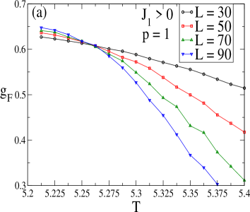
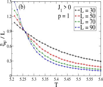
Figure 1: (a) Binder Cumulant; (b) and the second-order correlation length using four lattice sizes, for fixed ferromagnetic $J_{1}$ and $J_{2}$ couplings (case $p=1$ in Eq.(2)). The scale invariance at the critical temperature is clearly seen at the crossing point in (a) and (b). The critical temperature is $T_{c}\approx 5.26$.

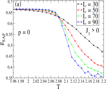
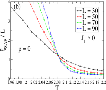
Figure 2: (a) Binder Cumulant; (b) and the second-order correlation length using four lattice sizes, for fixed ferromagnetic $J_{1}$ and antiferromagnetic $J_{2}$ couplings (case $p=0$ in Eq.(2)). Note that the critical temperature is close to $T=2.08$ (see reference malakis_2006 ).

For $p=1$, we have the trivial case of the Ising model in the square lattice with nearest- and next-nearest-neighbor interactions having a second-order phase transition at $T_{c}=5.262\pm 0.001$ (in agreement with reference dalton_1969 ). For $p=0$, the SAF phase is present at low temperatures, and the SAF-P transition is found at $T=2.083\pm 0.002$ (the same value was obtained in malakis_2006 ). Figures 1 and 2 show how these values were determined by locating the crossing point of respective Binder Cummulant and correlation length. It is important to point out that the present curves of the second moment correlation length are only valid for $T\geq T_{c}$, but for the sake of visualization they are plotted for $T<T_{c}$ too. Of course, the criticality for $p=0$ and $p=1$ is reached at equilibrium, since no competing kinetics takes place.

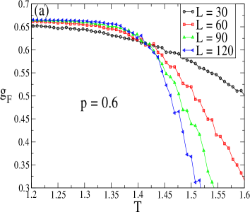
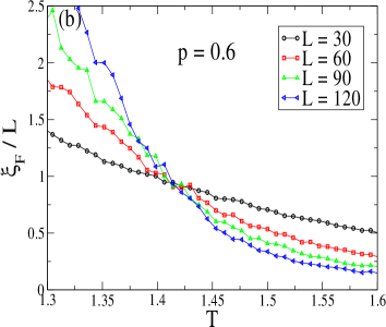
Figure 3: (a) Binder Cumulant; (b) and the second-order correlation length using four lattice sizes, for fixed ferromagnetic $J_{1}$ couplings, and random $J_{2}$ couplings obeying the PDF given in Eq.(2), for $p=0.6$. This is a nonequilibrium critical steady state. The scale invariance at the critical temperature is clearly seen at the crossing point in (a) and (b).

The role of $p$, for $0<p<1$, is to create a competition between SAF and F, which is stronger for its intermediate values (see Eq.(2)). When $p$ is close to 1, the ferromagnetic order is present as Fig.3 shows. There it is observed the Binder Cummulant $g_{F}$ and the second moment correlation length divided by the lattice size $\xi_{F}/L$ as functions of the temperature, corresponding to the ferromagnetic order parameter $m_{F}$, for $p=0.6$. Four curves, for sizes $L=30,60,90,120$, colapse at a point in Fig.3(a) and (b) locating the critical temperature. Both figures agree with the value $T_{c}=1.410\pm 0.005$. This is a clear signal of second-order phase transition. However, the scale invariance at the critical point seems to be better visualized using the correlation length.

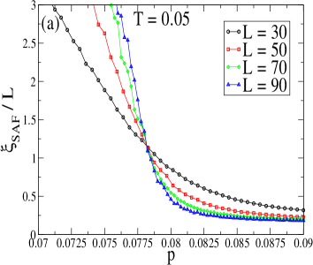
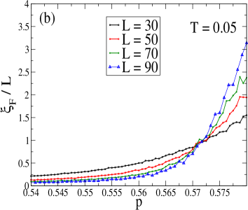
Figure 4: Correlation length scanned at a fixed very low temperature, for fixed ferromagnetic $J_{1}$ couplings, and random $J_{2}$ couplings obeying the PDF given in Eq.(2). In (a) the critical probability of the SAF-P transition is about $p=0.078$. In (b) the critical probability of the F-P transition is about $p=0.57$.

In Fig.4 is shown the correlation length $\xi_{SAF}$ and $\xi_{F}$ scanned through the probability $p$, for a very low temperature $T=0.05$. In Fig.4a the crossing point is located at $p_{c}=0.0783\pm 0.0004$, whereas in Fig.4b we have $p_{c}=0.571\pm 0.006$. Consequently, there is a paramagnetic gap between the SAF-P and F-P second-order frontiers. In Fig.5 the resulting phase diagram is exhibited, where all points were obtained using the correlation length and the Binder Cummulant. Note the paramagnetic gap for $p_{c1}\leq p\leq p_{c2}$, where $p_{c1}\approx 0.078$ and $p_{c2}\approx 0.57$.

If $J_{2}$ obeys the PDF given in Eq.(3) (a double Gaussian), any finite value of the standard deviation $\sigma$ destroys the SAF phase. In what follows, $\sigma$ will be expressed in units of $J_{1}$. Note that the PDF given in Eq.(2) is the limit of the double Gaussian given in Eq.(2), when $\sigma\to 0$. Interestingly, the effect of a very small $\sigma$ is to shift the extreme critical points of the phase diagram from $p_{c}\approx 0.57$ to $p_{c}\approx 1/3$ and from $T_{c}(p=1)\approx 5.26$ to $T_{c}(p=1)\approx 3.57$. We confirmed that this shift exists even for a very small value of $\sigma$, such as $\sigma=0.001$.

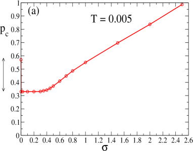
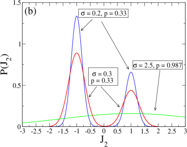
Figure 7: (a) The critical probability of the phase diagram shown in Fig6 versus the parameter $\sigma$ given in Eq.(3). Note the discontinuous fall in $p_{c}$ when $\sigma$ assumes a finite value. In (b) is shown the PDF given in Eq.(3) for three different values of the pair ($p$, $\sigma$). Note that there is a weak overlap of the two peaks, for $p_{c}=0.33$ and $\sigma=0.3$ causing the first inflection point in the curve shown in (a). For $p_{c}=0.987$ and $\sigma=2.5$ the left gaussian is just irrelevant, and the right one is very extended.

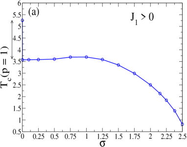
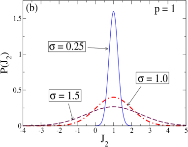
Figure 8: (a) The critical temperature of the phase diagram shown in Fig6 versus the parameter $\sigma$ given in Eq.(3), for $p=1$. Note the discontinuous fall in $T_{c}$ when $\sigma$ assumes a finite value. In (b) is shown the PDF given in Eq.(3) for three different values of $\sigma$, for $p=1$. Note that the critical temperature reaches its maximum for $\sigma=1$, and decreases when the left tail of the gaussian include more negative values of $J_{2}$.

In Fig.5 the phase diagram is presented for $\sigma=0.1$. There, the extreme points of the frontier are $p_{c}=0.3310\pm 0.0005$, for $T=0.005$, and for $p=1$, $T_{c}=3.5730\pm 0.0004$. To understand the effect of the standard deviation on $p_{c}$ we show in Fig7a how $p_{c}$ evolves with $\sigma$. It remains constant for $0<\sigma<0.3$, because the gaussians of the PDF do not overlap, as Fig7b shows. Then, it increases from $\sigma\approx 0.3$, since the gaussians of the PDF increases their overlap. For $\sigma=2.5$, $p_{c}=0.987$(see Fig7b). Accordingly, for $\sigma\gtrsim 2.5$, $p_{c}$ reaches its maximum value, which is one. So, the ferromagnetic area of the phase diagram is totally reduced, since the randomness caused by $\sigma$ is so strong, such that any amount of the second Gaussian in Eq.(3) (any amount of ($1-p$)), would destroy the ferromagnetic phase (see Fig7). On the other hand, the effect of $\sigma$ on $T_{c}(p=1)$ is presented in Fig.8.

In Fig.8a it can be observed the discontinuous fall in the critical temperature $T_{c}(p=1)$ when $\sigma$ assumes infinitesimal values, remaining constant for $0<\sigma<0.5$. Then it increases slightly before reaching its maximum for $\sigma\approx 1$. Then $T_{c}(p=1)$ decreases. The extension of the Gaussian distribution for these three different stages is exhibited in Fig.8b, for three representative values of $\sigma$. Note that the critical temperature is unaltered when the probability for negative values of $J_{2}$ is zero. However, if the left tail of the Gaussian includes the interval $-2\lesssim J_{2}<0$, $T_{c}(p=1)$ increases. If this interval of negative $J_{2}$ values is extended, the effect of $\sigma$ is to decrease the critical temperature. In Fig.8a the critical temperature is plotted up to $\sigma=2.5$, when $p_{c}$ assumes the value 1.

III.2 Case where $J_{1}<0$

Now we treat the case $J_{1}<0$, where the nearest-neighbor interactions are antiferromagnetic. If the PDF given in Eq.(5) is obeyed by the $J_{2}$ bonds, these are antiferromagnetic with probability $1-p$, and zero with probability $p$. So, $p$ measures the degree of dilution of $J_{2}$ bonds. This particular case was studied in equilibrium with quenched randomness in reference yining_2018 , where $x$ stood for our probability of dilution $p$, as mentioned before in the Introduction.

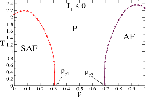
Figure 9: Phase diagram of the model given by the Hamiltonian given in Eq.(1), for fixed antiferromagnetic $J_{1}$ interactions, and random $J_{2}$ bonds obeying the PDF given in Eq.(5). The maxima at both frontiers are not present in the equivalent phase diagram of Fig.5a of reference yining_2018 , which was obtained with quenched randomness at equilibrium.

The phase diagram we obtained is shown in Fig.9, where the SAF-P and AF-P frontiers are separated by paramagnetic gap for $p_{c1}\leq p\leq p_{c2}$, where $p_{c1}\approx 0.309$ and $p_{c2}\approx 0.69$. The critical temperatures at the extremes of the phase diagram are $T_{c}(p=0)\approx 2.08$ (in agreement with malakis_2006 ), and $T_{c}(p=1)=2.269...$ (the exact 2D Ising one).

Phase diagram in Fig.9 can be compared with that exhibited in Fig.5a of reference yining_2018 . There, the Neel phase is our AF phase and the strip antiferromagnetic one is our SAF phase. The topology is quite similar. Nevertheless, we did not find a spin-glass phase in the gap area close to $T=0$, as in reference yining_2018 . At least, not with the spin-glass order parameter averaging the correlation between the spins of two copies of the system (see Eq.(6) in yining_2018 ).

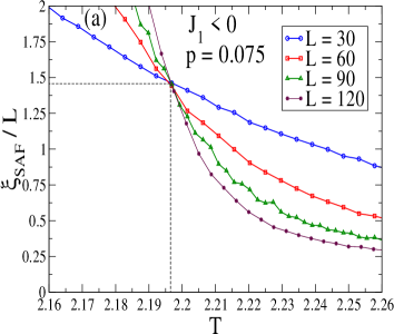
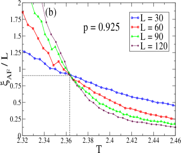
Figure 10: (a) Curves of $\xi_{SAF}/L$, where the crossing point is at $T=2.196\pm 0.003$ (above $T_{c}(p=0)$); (b) Curves of $\xi_{AF}/L$, where the croosing point is at $T=2.364\pm 0.004$ (above $T_{c}(p=1)$). These two crossing points correspond to the maximum of each frontier in Fig.9. Furthermore, in (a) $\xi_{SAF}/L$ is $1.467\pm 0.008$ at the point of intersection , whereas in (b) $\xi_{AF}/L$ is $0.904\pm 0.003$ (which is the Ising universal amplitude $x^{*}$ salas2000 ). Dashed lines are guides to the eye.

Furthermore, the frontiers we obtained exhibit humps, which do not appear with quenched randomness in that paper. In the present case, the SAF-P frontier reaches its maximum at $(p,T_{c})\approx(0.075,2.196)$, and at $(p,T_{c})\approx(0.925,2.364)$, for the AF-P frontier, as shown in Fig.10. These humps may be caused by the particular type of competing kinetic used in this work, which causes an increase of the critical temperature for values of $p$ close to zero and $1$.

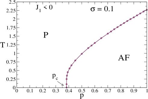
Figure 11: Phase diagram for fixed antiferromagnetic $J_{1}$ bonds, and random $J_{2}$ interactions obeying the PDF given in Eq.(6), when $\sigma=0.1$. The horizontal axis is the probability $p$, which is the weight of the first gaussian in Eq.(6). There is only one frontier separating the AF and P phases. The SAF phase can not be formed for $\sigma\neq 0$.

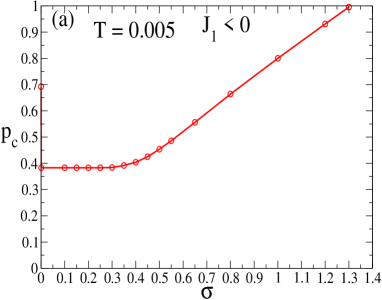
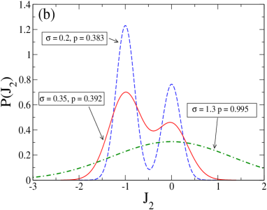
Figure 12: (a) The critical probability of the phase diagram shown in Fig11 versus the parameter $\sigma$ given in Eq.(6). Note the discontinuous fall in $p_{c}$ when $\sigma$ assumes a finite value. In (b) is shown the PDF given in Eq.(6) for three different values of the pair ($p$, $\sigma$).

Finally, we applied the PDF given in Eq.(6) for the $J_{2}$ bonds, with $J_{1}<0$. In this case $J_{2}$ is distributed by two gaussians centered at $J_{2}=0$ and $J_{2}=J_{1}$, with probability $p$ and $1-p$, respectively. When $\sigma\to 0$ the bimodal given in Eq.(5) is recovered. In Fig11 is presented the phase diagram for $\sigma=0.1$. Again we observe that the SAF is not present. This happens even when $\sigma$ is infinitesimal. Thus, only the AF survives in an area enclosed by a second-order frontier, where $p_{c}\approx 0.692$ and $T_{c}(p=1)$ is the 2D Ising critical temperature. The evolution of $p_{c}$ with $\sigma$ is shown in Fig.12a, where we may see how $p_{c}$ falls from $p_{c}\approx 0.692$ down to $p_{c}\approx 0.383$, when $\sigma$ assumes an infinitesimal value. Then, $\sigma$ does not affect the value of $p_{c}$ until $\sigma\gtrsim 0.35$.

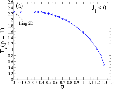
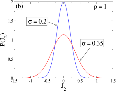
Figure 13: (a) The critical temperature of the phase diagram shown in Fig11 versus the parameter $\sigma$ given in Eq.(6), for $p=1$. Note that $\sigma$ does not affect the value of the critical temperature for $\sigma\lesssim 0.35$. In (b) is shown the PDF given in Eq.(6) for two different values of $\sigma$, for $p=1$. Note that the tails of the gaussian for $\sigma=0.35$ include $|J_{2}|>1$, whereas for $\sigma=0.2$ they die for $|J_{2}|<1$.

The AF area disappears when $p_{c}=1$, this happens for $\sigma\gtrsim 1.3$. In Fig.12b is shown that $p_{c}$ is not affected by $\sigma$ when the tails of the two gaussians die for $-1<J_{2}<1$. For $\sigma\lesssim 0.35$, the tails of the two gaussians start to include $|J_{2}|>1$, so $p_{c}$ begins to increase. Similarly, in Fig.13 is shown the evolution of $T_{c}(p=1)$ with $\sigma$, until $p_{c}$ reaches the value 1. It confirms that the frontier exhibited in Fig.11 is unaltered when $\sigma<0.35$.

III.3 The amplitude $x^{*}_{SAF}$

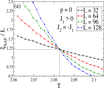
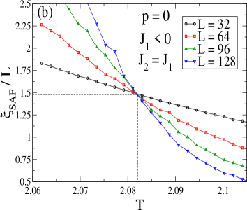
Figure 14: Curves of the correlation length for different sizes of the lattice. Curves in (a) and (b) intercept at the critical temperature of the SAF-P transition in Figures 5 and 9, for $p=0$, respectively. In (a) the crossing point is observed at $(2.0832\pm 0.0006,1.210\pm 0.005)$ ; In (b) it is at $(2.082\pm 0.001,1.483\pm 0.008)$. Dashed lines are guides to the eye, through which we may note that $x^{*}_{SAF}$ is different in (a) and (b).

The amplitude $x^{*}_{SAF}$ in Eq.(16) has attracted our attention. We may observe that the crossing point of $\xi_{SAF}/L$ curves gives different values of $x^{*}_{SAF}$ when $J_{2}=-J_{1}<0$ and $J_{2}=J_{1}<0$. This is exhibited in Fig.14, where the point of intersection provides $T_{c}(p=0)$ in Figures 5 and 9. In Fig.14a the uncertainty of the crossing point also gives $x^{*}_{SAF}=1.210\pm 0.005$, and in Fig.14b $x^{*}_{SAF}=1.483\pm 0.008$. However, the critical temperatures are just the same $T_{c}(p=0)\approx 2.082$, whithin the error.

So, though both critical points are just at the same SAF-P critical temperature, the way $J_{1}$ and $J_{2}$ bonds are configured to form the SAF phase gives a slight different value of $x^{*}_{SAF}$. To reinforce this idea, we analysed the effect of the bimodal distributions given in Eqs.(2) and (5) on this superanfiterromagnetic amplitude. For the case $J_{1}>0$, the SAF phase is destroyed for a small value of $p$ (see Fig. 5), so no relevant change in $x^{*}_{SAF}$ is observed. However, when $J_{1}<0$, the degree of dilution of $J_{2}$ changes this amplitude, as suggested by an ad-hoc finite-size criterium.

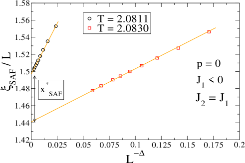
Figure 15: Extrapolation of $\xi_{SAF}/L$ to determine the amplitude $x^{*}_{SAF}$ for $L\to\infty$ (see the intercepts at the vertical axis). It is based on Eq.(16). The lines correspond to the limits of the interval of the uncertainty of $T_{c}$ (read the caption of Fig.14b). Therefore, the points between the intercepts are $1.440<x^{*}_{SAF}<1.497$.

To show it, we have determined the interval of uncertainty of $x^{*}_{SAF}$ in Fig.15, for $p=0$, using Eq.(16). We used small sizes of $L$, such as $L=8,10,12,14,16,18,20,24,28$, for which the second term in Eq.(16) is relevant. The limits of $x^{*}_{SAF}$ were determined by extrapolating to $L\to\infty$ the line of points of $\xi_{SAF}/L$ versus $L^{-\Delta}$, each one corresponding to the limits of the critical temperature found in the crossing point of Fig.14b.

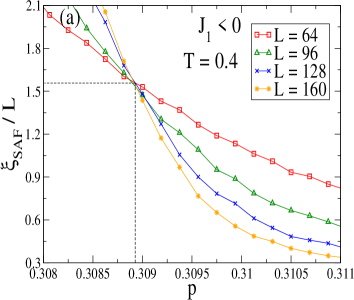
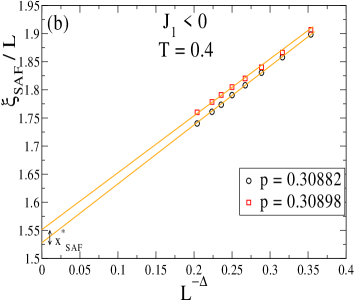
Figure 16: In (a) the uncertainty of the crossing point gives the critical probability $p$ of the PDF in Eq.(5), in the interval $0.30882<p_{c}<0.30898$. In (b) the limits of the uncertainty of $x^{*}_{SAF}$ are determined by extrapolating $\xi_{SAF}/L$ to $L\to\infty$, for each limit of $p_{c}$. So we have $1.53<x^{*}_{SAF}<1.55$. This interval does not intersect that of Fig.15.

The values of $\Delta$ were scanned in order to get the adequate ones to adjust the points in a straight line. So, the two extrapolated lines in Fig.15 intersect to the vertical axis at points which constitute the limits of the uncertainty of $x^{*}_{SAF}$. Accordingly, we found $1.440<x^{*}_{SAF}<1.497$. A similar extrapolation was performed for the transition point at $T=0.4$ of the left frontier in Fig.9. There we have $0.30882<p_{c}<0.30898$, according to the uncertainty of the crossing point shown in Fig. 16a.

The resulting interval of the amplitude is shown in Fig.16b. Thus, $1.53<x^{*}_{SAF}<1.55$, which does not intersect the interval found for $p=0$. Therefore, this finite-size analysis suggest that $x^{*}_{SAF}$ also changes with the dilution of $J_{2}$. Of course, more rigorous numerical treatments need to be done to confirm this affirmation.

IV Conclusions

We have studied the steady states of a nonequilibrium $J_{1}-J_{2}$ Ising model with random $J_{2}$ bonds obeying bimodal and double Gaussian probability distribution functions, for ferromagnetic and antiferromagnetic $J_{1}$ couplings, in a competing kinetics.

All the phase diagrams presented second-order frontiers dividing the paramagnetic phase (P) with some of the following orders : the F, AF or SAF order. Other authors found similar topologies for these phase diagrams obtained at equilibrium using quenched randomness with the bimodal distributions considered in this work. We observed that the SAF phase can not exist when $J_{2}$ obeys a continuous probability distribution.

Also, no universality breaking was observed for the critical exponents of the corresponding order parameters and their susceptibilities. However, we found that the amplitude $x^{*}_{SAF}$ of the correlation length at the SAF-P transition is not only different to that of 2D pure Ising model, but may change if the degree of dilution of $J_{2}$ bonds is relevant. This was shown by calculating the uncertainties of $x^{*}_{SAF}$. As far as we know, no other work has calculated this particular amplitude. It would be interesting to perform the same calculations with quenched randomness in order to compare the obtained $x^{*}_{SAF}$ values. This will be done in a future work.

ACKNOWLEDGEMENTS

This work was partially supported by CNPq - Grants: 408787/2018-0 and 306569/2018-3 (Brazilian Research Agency). We also thank Ivan Scivetti for fruitful discussion.

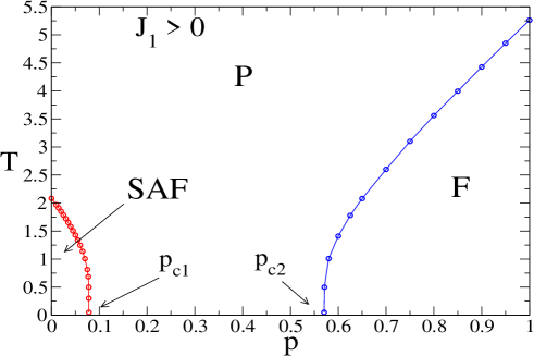
Figure 5: Phase diagram of the model given by the Hamiltonian given in Eq.(1), for fixed ferromagnetic $J_{1}$ couplings, and random $J_{2}$ bonds obeying the PDF given in Eq.(2). Critical points for $p=0$ and $p=1$ are at equilibrium, whereas for $0<p<1$, the frontier points are at nonequilibrium steady states.

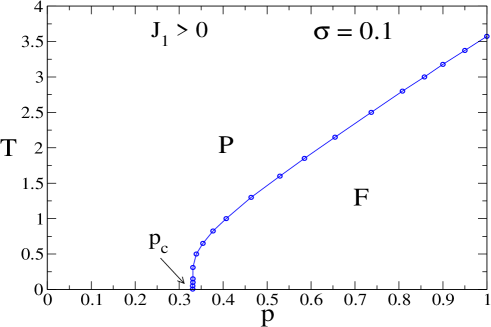
Figure 6: Phase diagram of the model given by the Hamiltonian given in Eq.(1), for fixed ferromagnetic $J_{1}$ couplings, and random $J_{2}$ bonds obeying the PDF given in Eq.(5), when $\sigma=0.1$. The vertical axis is the temperature and the horizontal one is the probability $p$, which is the weight of the first gaussian in Eq.(3). There is only one frontier separating the F and P phases, since any amount of $\sigma$ causes de destruction of the SAF phase.

References

- (1) Svetislav Mijatović, Dragutin Jovković, and Djordje Spasojević, Phys. Rev. E 103, 032147 (2021).
- (2) P. L. Garrido and J. Marro, Europhys. Lett. 15, 375 (1991).
- (3) A. I. López-Lacomba and J. Marro, Phys. Rev. B 46, 8244 (1992).
- (4) J. M. Gonzalez-Miranda, A. Labarta, M. Puma, Julio F. Fernández, P. L Garrido and J. Marro, Phys. Rev. E 49 2041 (1994).
- (5) N. Crokidakis, J. Stat. Mech. P02058 (2009).
- (6) N. Crokidakis, Phys. Rev. E 81, 041138 (2010).
- (7) P. Villa Martín, Juan A. Bonachela, and Miguel A. Muñoz. Phys. Rev. E 89, 012145 (2014).
- (8) Björn Ahrens and Alexander K. Hartmann, Phys. Rev. B 83, 014205 (2011).
- (9) M. P. Nightingale, Phys. Lett. A 59, 486 (1977).
- (10) R. H. Swendsen and S. Krinsky, Phys. Rev. Lett. 43, 177 (1979).
- (11) J. Oitmaa, J. Phys. A: Math. Gen. 14, 1159 (1981).
- (12) K. Binder and D. P. Landau, Phys. Rev. B 21, 1941 (1980).
- (13) D. P. Landau, Phys. Rev. B 21, 1285 (1980).
- (14) D. P. Landau and K. Binder, Phys. Rev. B 31, 5946 (1985).
- (15) D. P. Landau and K. Binder, Monte Carlo Simulations in Statistical Physics, 1st ed. (Cambridge University Press, Cambridge, 2000).
- (16) A. Kalz, A. Honecker, and M. Moliner Phys. Rev. B 84, 174407, (2011).
- (17) Yining Xu and Dao-Xin Yao Phys. Rev. B 97, 224419 (2018).
- (18) R. H. Swendsen and J. S. Wang, Phys. Rev. Letters 57, 2607 (1986).
- (19) David J. Earl and Michael W. Deem Phys. Chem. Chem. Phys. 7, 3910 (2005).
- (20) F. D. Nobre, Phys. Rev. E 64, 046108 (2001).
- (21) L. A. Fernandez, E. Marinari, V. Martin-Mayor, G. Parisi, and J. J. Ruiz-Lorenzo Phys. Rev. B 94, 024402 (2016).
- (22) Octavio. D. R. Salmon, J. Ricardo de Sousa and F.D. Nobre, Phys. Lett. A, 373, 2525 (2009).
- (23) Helmut G. Katzgraber, I. A. Campbell, and A. K. Hartmann, Phys. Rev. B 78, 184409 (2008).
- (24) Ian A. Campbell and Perch Lundow, Entropy 21, 978 (2019).
- (25) J. Salas, and A. D. Sokal, J. Stat. Phys. 98, 551 (2000).
- (26) E. J. Flores-Sola, B. Berche, R. Kenna and M. Weigel, Eur. Phys. J. B. 88, 28 (2015).
- (27) L. Jones and A. P. Young, Phys. Rev. B 71, 174438 (2005).
- (28) N. W. Dalton and D. W. Wood, J. Math. Phys. 10, 1271 (1969).
- (29) A. Malakis, P. Kalozoumis and N. Tyraskis, Eur. Phys. J. B 50, 63 (2006).