Distribution-aware Margin Calibration for Semantic Segmentation in Images

Abstract

The Jaccard index, also known as Intersection-over-Union (IoU), is one of the most critical evaluation metrics in image semantic segmentation. However, direct optimization of IoU score is very difficult because the learning objective is neither differentiable nor decomposable. Although some algorithms have been proposed to optimize its surrogates, there is no guarantee provided for the generalization ability. In this paper, we propose a margin calibration method, which can be directly used as a learning objective, for an improved generalization of IoU over the data-distribution, underpinned by a rigid lower bound. This scheme theoretically ensures a better segmentation performance in terms of IoU score. We evaluated the effectiveness of the proposed margin calibration method on seven image datasets, showing substantial improvements in IoU score over other learning objectives using deep segmentation models.

1 Introduction

Semantic segmentation in images is a fundamental yet challenging problem in computer vision. The task is to build a computational model to accurately assign a class label to every pixel. Semantic segmentation has drawn a broad research interest for many applications such as robotic sensing Cadena and Košecká (2014) and auto-navigation Xiao and Quan (2009). Recently, the development of deep convolutional neural networks has led to remarkable progress in semantic segmentation due to their powerful feature representation ability to describe the local visual properties. Deep parsing networks are often fine-tuned based on the pre-trained classification networks, e.g., deep residual networks He et al. (2016).

To train a reliable deep learning model for semantic segmentation, the learning objective is one of the most critical ingredients. The most straightforward way is to treat the semantic segmentation as a dense classification task, which examines each pixel in images individually, comparing the class-predictions to the one-hot encoded ground truth. As a surrogate relaxation of the mis-classification rate, cross-entropy becomes the most intuitive loss function in training deep semantic segmentation models. The minimization of cross-entropy is directly related to the maximization of pixel accuracy. In the training process, cross-entropy loss averages over all pixels in images, which is essentially asserting equal learning to each pixel in an image batch. This is problematic in semantic segmentation if the actual classes are imbalanced in the image corpus, as training can be dominated by the most prevalent class, e.g., the small foreground interest regions are submerged by large background areas. Although applying a cost-sensitive re-weighting scheme Wong et al. (2018) to alleviate the data imbalance and emphasize the “important” pixels, it is unclear how to determine the weights for the best IoU scores Ma et al. (2021), because the pixels of minority class do not necessarily mean they are difficult to be classified (see the ablation study in Section 4.3). Furthermore, the measure of cross-entropy on the validation set is a poor indicator of the model quality Berman et al. (2018), as minimizing the pixel-wise loss cannot guarantee a higher IoU score, which is more commonly used in semantic segmentation and can better sketch the contours of interest regions. To address these issues, some recently proposed loss functions have been proposed, e.g., Focal loss Lin et al. (2017) and Lovász-softmax Berman et al. (2018). The focal loss is an improved cross-entropy loss that tries to handle the class imbalance problem by assigning more weights to hard or easily misclassified examples and down-weight easy examples. The Lovász-softmax is a Lovász surrogate that mimics the IoU, making it consistent with the evaluation metric in semantic segmentation.

A “better” machine learning model should feature a better-generalized performance, i.e., the performance measured on the underlying data distribution, where the unknown instances are sampled from. Clearly, there is a gap between the empirical performance on the training dataset and the generalized performance regarding IoU, i.e., there always exists the IoU differences between training and validation datasets. This gap is commonly called the generalization error. Even though some regularization schemes have been applied to the training of neural networks, their influence on the generalization error of IoU still remains unclear. In this work, we explicitly show how this generalization error is related to label distribution and can be controlled by adding some class-dependent bias terms in the output of the deep semantic segmentation network. These bias terms are connected to the margins among multiple classes, where we are inspired by the idea of margins from the well-known Support Vector Machines (SVMs) Boser et al. (1992). In Blaschko and Lampert (2008), the authors proposed to apply the structured regression to predict the bounding box for object localization. For data-imbalanced learning problems, uneven margins can be applied to well calibrate the importance of specific classes Li et al. (2002); Khan et al. (2019); Cao et al. (2019). In semantic segmentation, class imbalance widely exists in most image datasets, which hinders the generalization ability of the model, because the IoU score for each class is jointly optimized with others. The power of the “uneven” margins inspires us to develop a proper margin calibration scheme for a better generalization ability of semantic segmentation models.

In this paper, we propose a novel distribution-aware margin calibration method, to optimize the IoU in semantic segmentation. The margins across multiple classes are pre-computed based on the label distribution, which can well calibrate the distance between foreground and background classes. Our method has the following three compelling advantages over other learning objectives: (1) it provides a lower bound for data-distribution IoU, which means the model has a guaranteed generalization ability; (2) the margin-offsets can be efficiently computed, which is readily pluggable into deep segmentation models; (3) the proposed learning objective is directly related to IoU scores, i.e., it is consistent with the evaluation metric. Due to the high discriminative power and stability, it is worth using the proposed margin calibration method as a learning objective in the challenging semantic segmentation tasks. We conduct extensive experiments on seven public image datasets, which indicates our method can achieve a considerable improvement compared to other learning objectives.

The rest of the paper is organized as follows. Section 2 introduces related work. Section 3 elaborates the proposed margin calibration method. Experimental results and analysis are presented in Section 4. Finally, Section 5 concludes the paper.

2 Related work

2.1 Deep learning-based semantic segmentation models

Deep learning-based image segmentation models have achieved significant progress on large-scale benchmark datasets Zhou et al. (2017); Cordts et al. (2016) in recent years. The deep segmentation methods can be generally divided into two streams: the fully-convolutional networks (FCNs) and the encoder-decoder structures. The FCNs Long et al. (2015) are mainly designed for general segmentation tasks, such as scene parsing and instance segmentation. Most FCNs are based on a stem-network (e.g., deep residual networks He et al. (2016)) pre-trained on a large-scale dataset. These classification networks usually stack convolution and down-sampling layers to obtain visual feature maps with rich semantics. The deeper layer features with rich semantics are crucial for accurate classification, but lead to the reduced resolution and in turn spatial information loss. To address this issue, the encoder-decoder structures such as U-Net Ronneberger et al. (2015) have been proposed. The encoder maps the original images into low-resolution feature representations, while the decoder mainly restores the spatial information with skip-connections. Another popular method that has been widely used in semantic segmentation is the dilated (atrous) convolution Yu and Koltun (2015), which can enlarge the receptive field in the feature maps without adding more computation overhead, thus more visual details are preserved. Some methods, such as DeepLab v3+ Chen et al. (2018), just combine the encoder-decoder structure and dilated convolution, to effectively boost the pixel-wise prediction accuracy.

2.2 Learning objectives for semantic segmentation

As a dense prediction task, the commonly used cross-entropy is a natural learning objective in training a semantic segmentation model. However, the classification accuracy is inconsistent with the evaluation metric IoU. In recent years, various learning objectives have been proposed specifically for semantic segmentation, and most of them can be used in a plug-and-play way. For example, the distribution-based loss functions (e.g., weighted cross-entropy loss Ronneberger et al. (2015) and focal loss Lin et al. (2017)), the region-based loss functions (e.g., IoU loss Rahman and Wang (2016), Dice loss Eelbode et al. (2020) and Tversky loss Salehi et al. (2017a)) and boundary-based loss functions (e.g., Hausdorff distance loss Karimi and Salcudean (2019) and Boundary loss Kervadec et al. (2019)). In medical image segmentation, Ma et al. presented a comprehensive review of 20 general loss functions Ma et al. (2021). These loss functions can also be jointly used in model optimization Abraham and Khan (2019). In deep learning based segmentation methods, the model outputs continuous class probabilities of all pixels, which are indirectly related to IoU scores. To deal with this problem, Maxim et al. proposed to use submodular measures to readily optimize the segmentation model in the continuous setting Berman et al. (2018). In many real application scenarios, especially scene parsing, the pixel-labels are highly imbalanced, so we prefer to balance the label weights among different classes. By adding down-weights to the well-classified records and assign large weights to misclassified records, focal loss can effectively boost the performance of dense prediction.

On the other hand, design proper surrogates as learning objectives is also applicable to mimic the IoU in semantic segmentation. For example, Nowozin proposed a statistical approximation based on parametric linear programming as a tractable decision making process Nowozin (2014). Ahmed et al. combine the expected-intersection over expected-union (EIoEU) with optimizing the expected-IoU (EIoU) for a set of candidate solutions Ahmed et al. (2015). For the deep learning based semantic segmentation, Nagendar et al. proposed to plug a surrogate network into the deep segmentation model for the approximation of IoU Nagendar et al. (2018), while such a scheme can be also extended to other non-decomposable evaluation metrics, e.g., miss-classification rate (MCR) and Average Precision (AP), in universal machine learning tasks Grabocka et al. (2019).

However, the above methods are mainly to minimize the empirical risk in the model training procedure, without the consideration of the generalization of IoU. In deep learning based segmentation tasks, one may directly use some general methods such as $l_{2}$-norm, weight-decay, drop-out or extensive data augmentation to improve the generalization ability, but it is unclear how or whether these methods are correlated to the generalization of IoU. As one of the critical objective in design machine learning models, optimizing the generalized performance can be achieved through (1) optimizing the empirical performance approximated by a surrogate loss associated with the performance metric Berman et al. (2018); Grabocka et al. (2019), e.g. IoU; and (2) controlling the generalized error. In our work, we design a margin calibration scheme with a proper loss function to overcome this difficulty, which provides a better learning objective for semantic segmentation compared to other learning metrics, both theoretically and practically.

3 Method

3.1 Problem setup and notations

Semantic segmentation in images is essentially a dense classification problem, where a model predicts the one-hot labels to distinguish each foreground class from the background class, using the definition of true positive ($TP$), false positive ($FP$) and false negative ($FN$). The Jaccard index (IoU) is defined as the size of intersection divided by the size of the union of the sample sets:

$$IoU=\frac{TP}{TP+FP+FN}.$$ (1)

In semantic segmentation, IoU is measured from the pixel-wise classifications, which differs from object localization, where IoU is calculated by the regression of bounding boxes Blaschko and Lampert (2008). In this paper, we do not consider the regression case.

A similar metric to IoU is Dice Similarity Coefficient (DSC), which is equivalent to F1-score:

$$DSC=\frac{2\times TP}{2\times TP+FP+FN}.$$ (2)

However, the above two metrics are count-based measures, whereas the outputs of deep segmentation models are probability values representing the likelihood of the pixels belonging different classes. Therefore, neither IoU score nor DSC can be directly and accurately measured from the output of the network.

For a multi-class semantic segmentation problem, we formally define an input space $\mathcal{X}\in\mathbb{R}^{w\times h\times c}$ and the target space $\mathcal{Y}=\{1,\ldots,K\}^{w\times h}$, where $w$, $h$, $c$ are the width, height and numbe of channels of an input image, and $K$ is the total number of classes to be segmented. For simplicity, we use $M=w\times h$ to represent the total number of pixels in an image. The function $\theta\in\Theta:\mathcal{X}\mapsto\mathcal{Y}$ is a complex non-linear projection from images to masks (pixel labels). In deep learning-based semantic segmentation methods, $\Theta$ can be a learning framework with trainable parameters.

Given an image $\mathbf{x}\in\mathcal{X}$ with a corresponding mask $\mathbf{y}\in\mathcal{Y}$, we denote the discrete predicted label for $i$-th pixel is $\hat{y}_{i}$. Then, given a ground truth $\mathbf{y}$ and a prediction $\mathbf{\hat{y}}$, the empirical IoU regarding the $k$-th foreground class is:

$$IoU_{k}=\frac{P_{k}-P_{k0}}{P_{k}+P_{0k}}.$$ (3)

where $P_{k0}$ denotes the empirical probability that a foreground class $k$ pixel is observed but is predicted as the background class by $\theta$, i.e.,

$$P_{k0}=\frac{1}{M}\sum\limits_{i=1}^{M}\mathbb{I}(y_{i}=k\wedge\hat{y}_{i}\neq k),$$ (4)

with $\mathbb{I}(\cdot)$ an indicator function. Similarly, $P_{0k}$ denotes the empirical probability that a pixel of the background class is observed but is predicted as the foreground class $k$, i.e.,

$$P_{0k}=\frac{1}{M}\sum\limits_{i=1}^{M}\mathbb{I}(y_{i}\neq k\wedge\hat{y}_{i}=k).$$ (5)

We use $P_{k}$ to denote the empirical probability that a class $k$ foreground pixel is observed, i.e.,

$$P_{k}=\frac{1}{M}\sum\limits_{i=1}^{M}\mathbb{I}(y_{i}=k).$$ (6)

In the evaluation of the segmentation performance, IoU is computed globally over an image dataset, in which the total number of pixels is $N$, where $N\gg M$. From the statistical perspective, we assume that the image samples in the whole dataset are independently and identically distributed (i.i.d) according to some unknown distribution $\mathcal{D}$ over $\mathcal{X}\times\mathcal{Y}$, and let $\mathcal{D}_{\mathcal{Y}}$ denote the projection of $\mathcal{D}$ over $\mathcal{Y}$. Note that we do not assume the pixels in an image are i.i.d. The IoU of $k$-th class over the whole data distribution is:

$$\mathpzc{IoU}_{k}=\frac{\mathpzc{P}_{k}-\mathpzc{P}_{k0}}{\mathpzc{P}_{k}+\mathpzc{P}_{0k}}.$$ (7)

Note that we use $P$ and $IoU$ of the normal font to represent the empirical probability and IoU on the finite image dataset, while use $\mathpzc{P}$ and $\mathpzc{IoU}$ of the calligraphic font to represent the probability and IoU over the whole data distribution.

When there are $K$ classes presented, the empirical mean IoU (mIoU) is defined as $mIoU=\frac{1}{K}\sum\limits_{k=1}^{K}IoU_{k}$, and similarly, the mIoU over the data distribution $\mathcal{D}$ is defined as $\mathpzc{mIoU}=\frac{1}{K}\sum\limits_{k=1}^{K}\mathpzc{IoU}_{k}$.

Ideally, a function $\theta$ should produce a high $\mathpzc{mIoU}$ over the data distribution to ensure the stable performance of $\theta$ on any data sampled from $\mathcal{D}$. Unfortunately, the data distribution $\mathcal{D}$ is usually fixed but unknown. Thus, we can only optimize the empirical mIoU, so that with a high probability it can lead to a high $\mathpzc{mIoU}$ over $\mathcal{D}$. The problem here is that how $mIoU$ and $\mathpzc{mIoU}$ are close to each other. Next, we present our method to minimize the error bound between $mIoU$ and $\mathpzc{mIoU}$, which can theoretically support the proposed margin calibration method.

3.2 Method overview

In semantic segmentation tasks, the label imbalance is an inherent issue for dense prediction, so equally treating all pixel labels in the model training may lead to the biased IoU scores towards the majority classes. Since in deep semantic segmentation models, the one-hot pixel labels of multiple classes are simultaneously optimized, the minority class may be still under-fitted when the majority class is already over-fitted. An intuitive approach is to set different weights to the loss function based on the number of pixels of each objective class, e.g., weighted cross-entropy. However, it is unclear if the weights of the loss functions based on the number of total pixels of the objective classes are optimal, because the “hardness” of segmenting the minority classes is not directly related to the number of training pixels. In our own experience, we found that weighted cross-entropy barely improves the model performance in terms of IoU.

In our approach, we instead set different margins for the pixel classes, which differs from the weight loss functions. Specifically, we would derive an optimal margin setting for a small error bound between $mIoU$ and $\mathpzc{mIoU}$. Denote the output score of $i$-th pixel in the image dataset regarding the $k$-th foreground class by $s_{ik}$. Here we define the margin for the $i$-th pixel with regard to class $k$ in the whole image set as:

$$\lambda_{ik}=s_{ik}-\max_{j\neq k}s_{ij}.$$ (8)

If the $i$-th pixel belongs to $k$-th foreground class, it is preferable to have a large positive value of $\lambda_{ik}$. Otherwise, we expect it to be a negative value. We then combine the margin $\lambda_{ik}$ with a $\rho$-margin loss function $\phi_{\rho}(\cdot)$ defined in (Mohri et al., 2018, Definition 5.5), to build the relationship between IoU score and the margin $\lambda_{ik}$. The $\rho$-margin loss is defined as:

$$\phi_{\rho}(\lambda)=\min\left(1,\max\left(0,1-\frac{\lambda}{\rho}\right)\right),$$ (9)

which encourages the margin $\lambda$ to be larger than $\rho$ and provides an upper bound for 0-1 loss, as is illustrated in Fig. 1. We call the parameter $\rho$ margin-offset. We can then bound the empirical probabilities $P_{k0}$ and $P_{0k}$ in Eq.(3) as:

$$P_{k0}(\theta) <\frac{1}{N}\sum\limits_{i\in Y_{k}}\phi_{\rho_{k0}}(\lambda_{ik})=\ell_{k0}(\theta,\rho_{k0}),$$ (10)

$$P_{0k}(\theta) <\frac{1}{N}\sum\limits_{i\in Y\setminus Y_{k}}\phi_{\rho_{0k}}(-\lambda_{ik})=\ell_{0k}(\theta,\rho_{0k}),$$

where we use $Y_{k}$ and $Y\setminus Y_{k}$ to denote the index set of the foreground pixels of $k$-th class and background pixels, respectively. $\rho_{0k}$ and $\rho_{k0}$ are pre-defined margin-offsets. Then, we can give a lower bound for Eq.(3) as:

$$\overline{IoU}_{k}=\frac{P_{k}-\ell_{k0}(\theta,\rho_{k0})}{P_{k}+\ell_{0k}(\theta,\rho_{0k})},$$ (11)

and the corresponding lower bound for $mIoU$ is:

$$\overline{mIoU}=\frac{1}{K}\sum\limits_{k=1}^{K}\overline{IoU}_{k}.$$ (12)

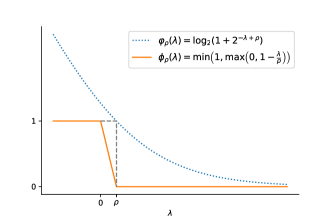
Figure 1: The $\rho$-calibrated log-loss (blue dotted line) and $\rho$-margin loss (orange solid line) functions. The $\rho$-margin loss is a upper bound for 0-1 loss. For the $\rho$-calibrated log-loss, $\varphi_{\rho}(\rho)=1$ and it upper bounds the $\rho$-margin loss.

3.3 Theoretical motivation

We can derive a generalization error bound regarding IoU with the margin-offsets $\rho_{k0}$ and $\rho_{0k}$, based on the following theorem:

Theorem 1.

For any function $\theta\in\Theta$, define $\mu_{k}=\frac{\rho_{k0}}{\rho_{0k}}$ and $\mathcal{F}=C(\Theta)+\sigma(\frac{1}{\eta})$. $C(\Theta)$ is some proper complexity measure of the hypothesis class $\Theta$ and $\sigma(\frac{1}{\eta})\triangleq\frac{\rho_{\max}}{4K}\sqrt{2M\log\frac{2K}{\eta}}$ is typically a low-order term in $\frac{1}{\eta}$ with $\rho_{\max}=\max\{\rho_{k0},\rho_{0k}\}_{k=1}^{K}$. Given a training dataset of $N$ image pixels including $N_{k}$ pixels of class $k$, with each image consisting of $M$ pixels, then for any $\eta>0$, with probability at least $1-\eta$,

$$\mathpzc{mIoU}\geq\overline{mIoU}-\epsilon,$$ (13)

where

$$\epsilon=\frac{1}{K}\sum\limits_{k=1}^{K}\frac{\sqrt{N-N_{k}}+\frac{\sqrt{N_{k}}}{\mu_{k}}}{\frac{N_{k}}{4K\mathcal{F}}\rho_{0k}-\sqrt{N-N_{k}}}.$$ (14)

Note that this theorem involves a complexity measure $\mathcal{F}=C(\Theta)+\sigma(\frac{1}{\eta})$, where $C(\Theta)$ is derived from the Rademacher complexity. The Rademacher complexity typically scales in $\sqrt{\frac{C(\Theta)}{N_{k}}}$ Mohri et al. (2018). Such a scale has been used in related works (see Cao et al. (2019); Neyshabur et al. (2018) and the references therein) to imply a connection between Rademacher complexity and number of pixels $N_{k}$. See the proof of the theorem in the appendix. This theorem enables us to maximize the $\mathpzc{mIoU}$ on the data distribution by maximizing a lower bound $\overline{mIoU}$ for the empirical IoU on a training dataset with a high probability. Meanwhile, we would prefer a small error bound $\epsilon$ so that the lower bound $\overline{mIoU}$ on the empirical IoU could be a reliable estimation for $\mathpzc{mIoU}$. This scheme guarantees the performance of associated function $\theta$ on the unseen image data.

Remark. At first glance, the relationship between $N$, $N_{k}$ and $\epsilon$ seems complicated. However, $\epsilon$ decreases if we increase $N$ and $N_{k}$ proportionally, as can be inferred from Eq. (14), so decreasing $\epsilon$ would need more these pixels accordingly. Theorem 1 indicates that a smaller $\epsilon$ requires more foreground class pixels, and a simple fit function for a smaller $C(\Theta)$. Another important factor is that we can adjust the margin-offset $\rho_{0k}$ to minimize the error bound $\epsilon$. Note that increasing $\rho_{0k}$ also increases the $C(\Theta)$ implicitly, because a larger margin-offset may require more complex hypothesis class $\Theta$. Otherwise, $\overline{mIoU}$ may decrease due to the under-fitting. Besides, the direct calculation of the optimal margin-offsets in Theorem 1 is difficult because it is related the complexity measure $C(\Theta)$, which is measured by the structure of deep neural networks. Nevertheless, we can give the optimal $\rho_{0k}$ that is irrelevant to $C(\Theta)$, by the following corollary:

Corollary 1.

Assume $\sum\limits_{k=1}^{K}\rho_{0k}=\text{some constant}.$ Let $\mu_{k}=\frac{P_{k}\sqrt{N_{k}}}{\upsilon(N-N_{k})-P_{k}\sqrt{N-N_{k}}}$ with $\upsilon$ ($\upsilon>0$) being a hyper-parameter. Then the minimum of the error bound $\epsilon$ in Theorem 1 is attained given the following condition:

$$\frac{\rho_{0i}}{\rho_{0j}}=\frac{N_{j}}{N_{i}}\frac{\sqrt{N-N_{i}}}{\sqrt{N-N_{j}}},\quad\frac{\rho_{k0}}{\rho_{0k}}=\mu_{k},\quad\forall i,j,k\in[1,K].$$ (15)

See the proof of the corollary in the appendix. Corollary 1 provides a theoretical guarantee for setting the margin-offsets towards a smaller error bound $\epsilon$. The margin-offset $\rho_{0k}$ is proportional to $\frac{\sqrt{N-N_{k}}}{N_{k}}$, which indicates a larger margin is required for $k$-th class, with comparably fewer pixels. We introduce a hyper-parameter $\tau$ ($\tau>0$) to scale the margin-offsets, which can be tuned on the validation dataset. Note that another margin $\rho_{k0}=\mu_{k}\rho_{0k}$ is usually small compared to $\rho_{0k}$ in practice with a well-tuned $\upsilon$, so we can mainly focus on $\rho_{0k}$ here. A proper setting of $\tau$ and $\upsilon$ can provide a balance between $\epsilon$ and $\overline{mIoU}$ for the maximization of $\mathpzc{mIoU}$. Empirically, just setting $\tau=10$ and $\upsilon=1$ can obtain a satisfactory result.

3.4 A practical implementation with $\rho$-calibrated log-loss function

Based on the above statistical analysis of label distribution, the learning objective needs to compute the margin-offsets from the whole pixel label set before optimizing the network. Given a pixel label set with $K$ classes, the computation of margin-offsets is summarized in Algorithm 1.

Algorithm 1 Margin-offsets calculation

Input: Labels for all pixels of size $N$. Number of pixels in each class given by $N_{1},...,N_{K}$. Hyper-parameter $\upsilon,\tau>0$.
Output: The margin-offsets $\rho_{0k}$, $\rho_{k0}$, $\forall k\in[1,K]$

1:for class $k=1,2,\ldots,K$ do

2:     $P_{k}=\frac{N_{k}}{N}$;

3:     $\mu_{k}=\frac{P_{k}\sqrt{N_{k}}}{\upsilon(N-N_{k})-P_{k}\sqrt{N-N_{k}}}$;

4:     $\rho_{0k}=\tau\times\frac{\sqrt{N-N_{k}}}{N_{k}}$;

5:     $\rho_{k0}=\mu_{k}\rho_{0k}$.

6:end for

The learning objective of semantic segmentation is to maximize $\mathpzc{mIoU}$ for the best performance. Ideally, we should maximize its lower bound $\overline{mIoU}$ with a small error bound $\epsilon$, because the margin-offset can provide a guarantee for its generalization. However, in the training of deep neural networks, the direct optimization of $\overline{mIoU}$ is impractical because the network is trained in a mini-batch manner. Unlike other decomposable evaluation metrics, such as classification accuracy, where the expectation of the metric on a mini-batch sample is equivalent to the metric on the whole dataset, the expectation of the mini-batch mIoU is an estimation to the overall mIoU on the whole dataset, i.e., the empirical IoU on the training dataset may be sub-optimal.

For a practical implementation, we instead minimize the sum of $\rho$-margin losses $l_{k0}$ and $l_{0k}$ involved $\overline{mIoU}$, with the optimal margin-offset. So for a mini-batch images, the loss $L(\theta)$ is calculated by:

$$L(\theta) =\sum\limits_{k=1}^{K}(\ell_{k0}(\theta,\rho_{k0})+\ell_{0k}(\theta,\rho_{0k}))$$

$$=\frac{1}{N_{s}}\sum\limits_{k=1}^{K}\left(\sum\limits_{i\in Y_{k}}\phi_{\rho_{k0}}(\lambda_{ik})+\sum\limits_{i\in Y\setminus Y_{k}}\phi_{\rho_{0k}}(-\lambda_{ik})\right),$$ (16)

with $\lambda_{ik}$ defined in Eq.(8), and $N_{s}$ is the number of pixels in a mini-batch. In the forward pass of training, the network $\theta$ outputs a batch of pixel-wise scores, in which the $i$-th pixel with regard to class $k$ is $s_{ik}$. Then $s_{ik}$ is used to calculate $\lambda_{ik}$ by Eq.(8).

In practice, the non-smoothness of $\rho$-margin loss function may bring instability in the optimization. As is shown in Fig. 1, the gradient regarding the $\rho$-margin loss can be prohibitively large when $\rho$ is very small, while the gradients outside the interval $(0,\rho)$ is zero. Thus, we substitute the $\rho$-margin loss $\phi_{\rho}(\lambda)$ used in Eq.(3.4) with $\rho$-calibrated log-loss $\varphi_{\rho}(\lambda)=\log_{2}(1+2^{-\lambda+\rho})$. The relationship between the $\rho$-margin loss $\phi_{\rho}(\lambda)$ and the $\rho$-calibrated log-loss $\varphi_{\rho}(\lambda)$ is illustrated in Fig. 1. Now we apply the margin-offsets to get a biased score $\bar{s}_{ik}$ for $\rho$-margin loss. The computation of $\bar{s}_{ik}$ is described in Algorithm 2.

Algorithm 2 $\rho$-margin calibration

Input: Prediction scores $\mathbf{s}=\{s_{ik}\}$, ground truth $y_{i}$, the margin-offset $\rho_{0k}$, $\rho_{k0}$, $\forall k\in[1,K]$ and $\forall i\in[1,N_{s}]$.
Output: $\rho$-margin calibrated prediction scores $\bar{\mathbf{s}}=\{\bar{s}_{ik}\}$.

1:for pixel $i=1,\ldots,N_{s}$ do

2:     for class $k=1,2,\ldots,K$ do

3:         $\lambda_{ik}=s_{ik}-\max\limits_{j\neq k}s_{ij}$,

4:         $\bar{s}_{ik}=\begin{cases}\lambda_{ik}-\rho_{k0}&\text{if}\quad y_{i}=k,\\ \lambda_{ik}+\rho_{0k}&\text{else}.\end{cases}$

5:     end for

6:end for

For the use of the $\rho$-calibrated log-loss $\varphi_{\rho}(\lambda)$, we first calibrate the output $\{s_{ik}\}$ via Algorithm 2, then the $\rho$-calibrated log-loss bounds the $\rho$-margin loss from above and leads to:

$$\ell_{k0}(\theta,\rho_{k0})\!<\!\frac{1}{N_{s}}\sum\limits_{i\in Y_{k}}\log_{2}(1\!+\!2^{-\bar{s}_{ik}})=\underline{\ell_{k0}}(\theta,\rho_{k0}),$$ (17)

and

$$\ell_{0k}(\theta,\rho_{0k})\!<\!\frac{1}{N_{s}}\sum\limits_{i\in Y\setminus Y_{k}}\log_{2}(1\!+\!2^{\bar{s}_{ik}})=\underline{\ell_{0k}}(\theta,\rho_{0k}).$$ (18)

Based on the above two inequalities, we simply use $\underline{\ell_{k0}}(\theta,\rho_{k0})$ and $\underline{\ell_{0k}}(\theta,\rho_{0k})$ to replace $\ell_{k0}(\theta,\rho_{k0})$ and $\ell_{0k}(\theta,\rho_{0k})$ in Eq.(3.4) as the final learning objective.

3.5 Complexity analysis

Given the output scores $\{s_{ik}\}^{N_{s}\times K}$ of $N_{s}$ pixels in an image batch, with the parallel computation provided by GPUs, calculating the margin $\lambda_{ik}$ needs $O(N_{s})$ time and $O(N_{s}K)$ space, and the subsequent calibrated log-loss incurs $O(N_{s}K)$ time complexity. So compared to the cross-entropy loss, the calibration method requires extra $O(N_{s}+N_{s}K)$ time and $O(N_{s}K)$ space complexities overhead in computing the calibrated log-loss.

3.6 Discussions

How to optimize non-decomposable loss like IoU is an open problem. This problem becomes far more challenging in the mini-batch training setting because in this case, we optimize the mini-batch IoU, which is an estimation of the overall IoU on the whole dataset. In our method, we mainly deal with a ratio distribution (both denominator and numerator of IoU are random variables regarding data distribution), where the central limit theorem can not be applied. As such, currently, no method can deal with this mini-batch setting accurately including lovász-softmax, which claims to be a surrogate for optimizing IoU. We also compromise on the learning objectives to optimize a related $\rho$-margin calibrated log-loss, which is independent of the margin calibration process. This makes our IoU on the training set a more reliable indicator for the IoU over the underlying distribution than other methods.

In the deep learning based semantic segmentation settings, directly applying margin calibration incurs additional space and time complexities. Consequently, the computation may be slower and more memory-consuming. To alleviate this, the network parameters can be initialized via training with cross-entropy, the most efficient but not the “perfect” learning objective, then fine-tuned with margin-calibration.

4 Experiment

In this section, we use the deep segmentation models to conduct the experiments on five publicly available datasets. Unlike the proposal of deep learning architectures that aims to achieve the best segmentation performance in some recent works Wang et al. (2020c); Shen et al. (2020); Ding et al. (2020), our contribution is mainly on the design of a novel learning method for better IoU scores when the learning framework is fixed. Given a deep segmentation model, we mainly compare the final performance when applying commonly used learning objectives and our margin calibration method.

4.1 Datasets

We conducted the experiment of semantic segmentation on seven datasets: Robotic Instrument Allan et al. (2019), COCO-Stuff 10K Caesar et al. (2018), PASCAL VOC2012 Everingham et al. (2015), MIT SceneParse150 Zhou et al. (2019), Cityscapes Cordts et al. (2016), BDD100K Yu et al. (2020) and Mapillary Vistas Neuhold et al. (2017).

The Robotic Instrument dataset provides 8 robotic surgical videos, in which 225 frames are sampled from each video. In the frames, each part is manually annotated by a trained team. Here we conduct the instrument part segmentation as an ablation study, in which we aim to correctly segment each articulating part of the instrument.

The COCO-Stuff 10K contains 9,000 images for training and 1,000 images for validation (testing). Following Ding et al. (2018), we evaluate the IoU performance on 171 categories (80 objects and 91 stuff) to each pixel.

The PASCAL VOC 2012 semantic benchmark contains 20 foreground object classes and one background class. The original dataset has 1,464 and 1,449 images for training and validation, respectively. To augment the training dataset, we also use extra annotations provided by Hariharan et al. (2011). The model is not pre-trained with MS COCO dataset.

The MIT SceneParse150 dataset is built based on ADE20K Zhou et al. (2017) as a scene parsing benchmark. It contains more than 20K scene images, annotated by 150 classes of dense labels. Here we use 2,000 validation images for qualitative evaluation.

The Cityscapes, BDD100K and Mapillary Vistas are three different street-view datasets. The data in Cityscapes were taken from 50 European cities, which provides fine-grained pixel-level annotations of 19 classes including buildings, pedestrians, bicycles, cars, etc. The training/validation/testing splits are with 2,975, 500 and 1,525 images, respectively. It also has 20,000 coarsely-labelled images, which can be used to pre-train the segmentation model.

Different from the Cityscapes dataset comes from Germany, the images of BDD100K are mainly from the US cities, and there is a dramatic domain shift between the two datasets for semantic segmentation models, although their labels are the same.

The Mapillary Vistas dataset contains 25,000 high-resolution images annotated into 66 fine-grained object categories, featuring locations from all around the world, and taken from a diverse source of image capturing devices.

4.2 Settings

We implemented the segmentation model based on PyTorch. For the experiment on the Robotic Instrument dataset, we applied the recently proposed COPLE-Net Wang et al. (2020a), a variant of U-Net Ronneberger et al. (2015) for medical image segmentation. COPLE-Net has much fewer trainable parameters compared to FCN, thus it is quite suitable for the segmentation tasks in a simple yet fixed application scenario. On the rest four datasets for general semantic segmentation tasks, we used DeepLab v3+ Chen et al. (2017) backend on SEResNeXt-50 Hu et al. (2018), with the output stride 8. We employed the AdamW optimizer Loshchilov and Hutter (2019) with the initial learning rate $10^{-4}$ in the training process. We used the mixed precision and gradient checkpoint, which allow to set a larger mini-batch size and can effectively save the GPU memory usage without hurting the batch normalization layers. Our experiments were conducted on a server equipped with a single NVIDIA Tesla V100 GPU card.

4.3 Ablation study on Robotic Instrument dataset

We sequentially split the Robotic Instrument dataset into 1,200, 200 and 400 images according to the frame index for training, validation and testing, respectively. For this task, we aim to accurately label four instrument parts, including shaft, wrist, claspers and probe. The pixel ratios in the 4 parts are 4.9%, 1.4%, 1.6% and 0.8%, respectively, while the background class occupies 91.2% of the total pixels, making the label distribution extremely imbalanced.

We used categorical cross-entropy as the baseline, as semantic segmentation can be treated as a dense prediction for each image pixel. In addition, we tested several recently proposed methods, including focal loss Lin et al. (2017) (with the scale factor 0.4), lovász-softmax Berman et al. (2018), generalized dice loss Sudre et al. (2017) and Tversky loss Salehi et al. (2017b). All these methods were used as independent learning objectives in the medical segmentation tasks, and the segmentation networks were all trained from the random state.

We recorded all the intermediate results during the training process, as is shown in Fig. 2. By observing these figures, we can see directly using the two count-based loss functions, Dice loss and Tversky loss, the segmentation network fails to converge, as they are not differentiable to pixel-wise categories and can only work in conjunction with distribution-based loss functions. The rest four methods show similar mIoU and loss curves. However, although lovász-softmax can utilize the sub-modular property to minimize the Jaccard loss, it is more likely to over-fit. The proposed margin calibration method can generally act as a plug-and-play learning objective like cross-entropy and focal loss in training a semantic segmentation network.

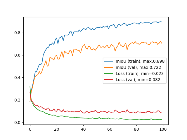
(a) Cross entropy

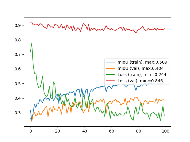
(b) Dice loss

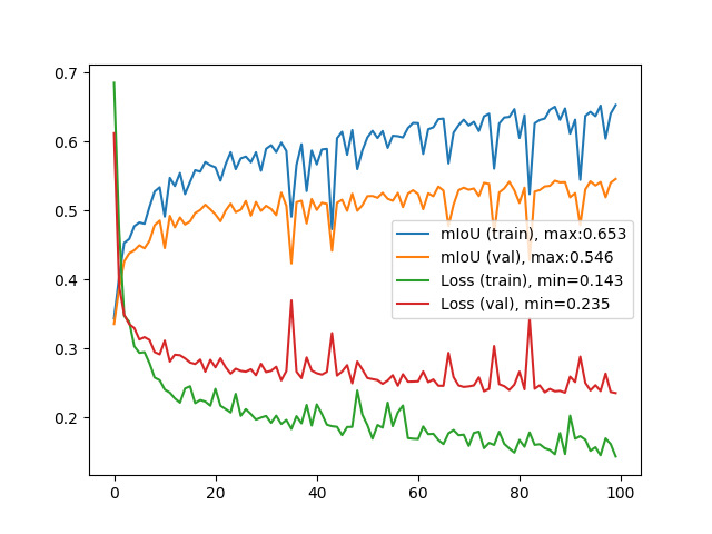
(c) Tversky loss

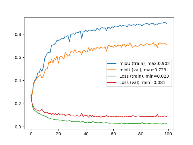
(d) Focal loss

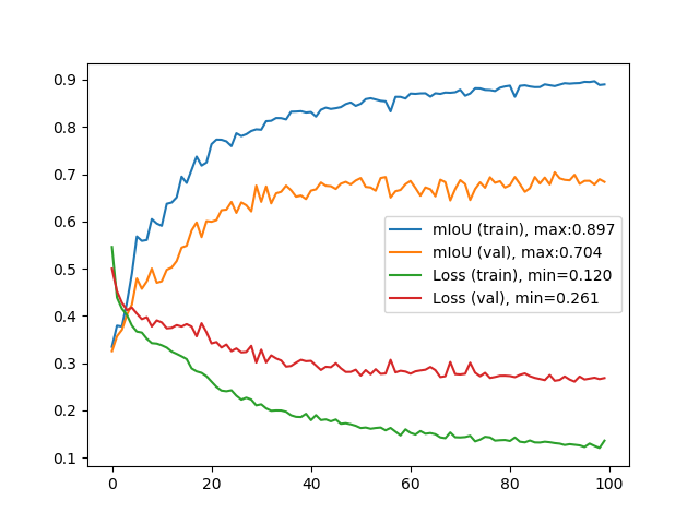
(e) Lovász-softmax

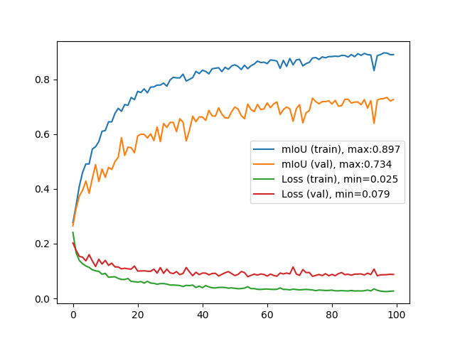
(f) Margin calibration

Figure 2: Training mIoU and loss curves on Robotic Instrument dataset.

In the model inference, we did not use horizontal flipping, multi-scale prediction or CRF post-processing to augment the segmentation performance. The quantitative results are shown in Table 1 and 2. The two evaluation metrics, pixel accuracy and IoU score, although have a very high correlation in terms of the absolute values, the best one single metric cannot guarantee the other. For example, simply using cross-entropy achieve a better pixel accuracy compared to the focal loss and lovász-softmax, but its IoU score is the worst. In semantic segmentation, the IoU score is usually a better evaluation to quantify the percent overlap between the pixel-label output and target mask. Using Dice loss as the learning objective, the model fails to segment shaft and claspers. Similarly, using Tversky loss cannot segment probe. Compared with cross-entropy, focal loss and Lovász-softmax, the proposed margin calibration method obtains the best pixel accuracy and IoU scores on this dataset. Specifically, as a single learning objective, margin calibration outperforms the second-best, with 3.0% performance gain in terms of the mIoU score. Although margin calibration is not specifically designed to optimize the pixel accuracy, it can also benefit from the generalization ability.

We illustrate the segmentation examples in Fig. 3. By observing the results, we can see that applying the proposed margin calibration method can effectively reduce the false positives, forming more smooth contours and obtaining more accurate results.

Table 1: The overall segmentation performance on the Robotic Instrument test set.

Method	Pixel Acc.	mIoU
Cross-entropy	81.1	66.2
Dice loss	38.3	27.3
Tversky loss	59.7	43.8
Focal loss	80.0	69.5
Lovász-softmax	80.1	68.9
Margin calibration	81.5	72.5

Table 2: Per-class IoU on the Robotic instrument test set.

Method	Shaft	Wrist	Claspers	Probe
Cross-entropy	81.1	55.3	55.5	72.9
Dice loss	0.0	58.1	0.0	72.6
Tversky loss	83.5	60.1	52.9	0.0
Focal loss	86.5	62.9	56.5	72.0
Lovász-softmax	86.3	64.4	55.5	69.3
Margin calibration	88.2	67.1	61.1	73.4

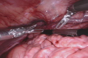
(a) Image

(b) Cross-entropy

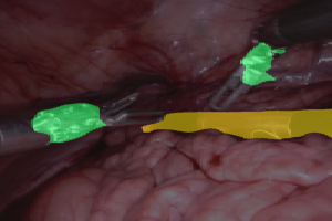
(c) Dice loss

(d) Tversky loss

(e) Focal loss

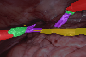
(f) Lovász-softmax

(g) Margin calibration

(h) Ground truth

Figure 3: Segmentation examples on the Robotic Instrument test set.

4.4 Results on COCO-Stuff 10K and PASCAL VOC2012 datasets

In the training of the segmentation model, we re-scaled the shorter image size to 400 then randomly cropped it to $384\times 384$. In the inference, we used the single-scale inference without flipping or any other augmentations. The comparisons on the two validation sets with the three baseline methods are reported in Table 3 and Table 4, respectively. Results show that when fixing the deep neural network, both focal loss and Lovász-softmax and improve the mIoU scores. By pre-computing the margin-offsets and applying the proposed margin calibration method, a single segmentation model can achieve a further 0.4% of the mIoU score on the COCO-Stuff 10K, while on the PASCAL VOC2012 dataset, the mIoU score with margin calibration is only 0.1% higher than the second-best.

By observing the two datasets, we found that they have different properties regarding pixel-label annotations. The dense prediction on the COCO-Stuff 10K dataset aims to auto-label all pixel classes, while on the PASCAL VOC 2012 the task is to distinguish one or two foreground objects from the unique background class. Also, the label imbalance in COCO-Stuff 10K is much more imminent than PASCAL VOC 2012, leading to the significant difference in margin calibrations. On the PASCAL VOC 2012 dataset, the background class void occupies 80% of the total pixels in the image corpus, while each foreground class has a very similar number of pixels (around 1%). So applying the $\rho$-margin calibration in Algorithm 2, the learning objective is more like a scaled log-loss.

Table 3: The segmentation performance on the COCO-Stuff 10K validation set.

Method	mIoU
Cross-entropy	34.1
Focal loss	34.9
Lovász-softmax	35.1
Margin calibration	35.5

Table 4: The segmentation performance on the PASCAL VOC2012 validation set.

Method	mIoU
Cross-entropy	78.2
Focal loss	78.3
Lovász-softmax	78.5
Margin calibration	78.6

4.5 Results on MIT SceneParse150 dataset

We experimented on the large-scale MIT SceneParse150 dataset to verify the effectiveness of the margin calibration method. Unlike the multi-task learning framework such as Xiao et al. (2018) to use multiple supervised information for the best segmentation performance, we only use the 150 scene labels and compare different single learning objectives in training the semantic segmentation model. The images were rescaled to $384\times 384$. On this dataset, we first used cross-entropy as the default learning objective to train the DeepLab v3+ model, then fine-tuned the network with focal loss, Lovász-softmax and the proposed margin calibration independently, to see the performance improvement of mIoU scores. The ground truth of the testing set has not been released, so we use the 2,000 validation images for qualitative evaluation. In the model inference, we adopted horizontal flipping and multi-scale prediction to augment the segmentation performance.

The comparisons on the validation set with the three baseline methods are reported in Table 5. Results show that when fixing the deep neural network, just using the proposed margin calibration method as a single learning objective, can boost the mIoU in very complex scene parsing tasks. When applying the flipping and multi-scale prediction, fine-tuning with focal loss and Lovász-softmax can improve the mIoU by 0.7% and 0.5%, respectively, while using the proposed margin calibration can achieve a further 0.9% of performance gain compared to categorical cross-entropy. Some example segmentation results in both indoor and outdoor environments are illustrated in Fig. 4. We can see compared to other learning objectives, applying margin calibration can better annotate the pillow, building exterior and sidewalk in these examples.

Table 5: The segmentation performance on the MIT SceneParse150 validation set.

Method	Flipping	Multi-scale	mIoU
			37.7
Cross-entropy	✓		37.9
	✓	✓	39.1
			37.9
Focal loss	✓		38.4
	✓	✓	39.8
			37.9
Lovász-softmax	✓		38.3
	✓	✓	39.6
			38.5
Margin calibration	✓		38.8
	✓	✓	40.2

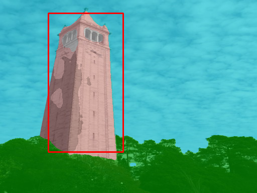
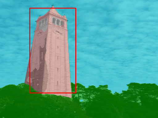
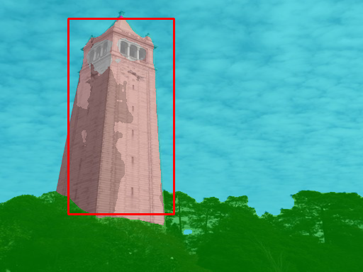
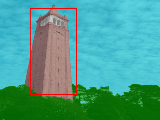
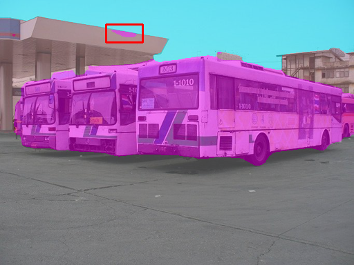
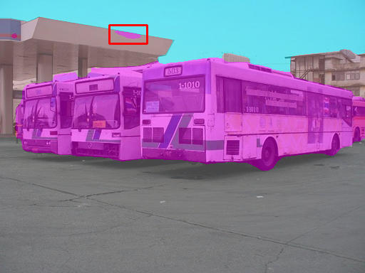
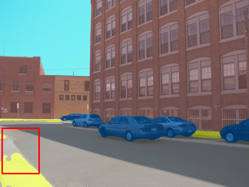
(a) Cross-entropy

(b) Focal loss

(c) Lovász-softmax

(d) Margin calibration

Figure 4: Scene parsing examples on MIT SceneParse150 validation set.

4.6 Results on Cityscapes, BDD100K, and Mapillary Vistas datasets

Table 6: The segmentation performance on the Cityscapes validation set (fine labels only).

Method	Flipping	Multi-scale	mIoU
			78.7
Cross-entropy	✓		78.9
	✓	✓	79.4
			78.9
Focal loss	✓		79.3
	✓	✓	80.6
			79.6
Lovász-softmax	✓		79.9
	✓	✓	80.5
			80.0
Margin calibration	✓		80.2
	✓	✓	81.1

Table 7: The segmentation performance on the BDD100K validation set.

Method	Flipping	Multi-scale	mIoU
			64.4
Cross-entropy	✓		64.6
	✓	✓	65.7
			64.5
Focal loss	✓		64.5
	✓	✓	65.8
			64.6
Lovász-softmax	✓		64.6
	✓	✓	65.8
			64.8
Margin calibration	✓		65.0
	✓	✓	66.1

Table 8: The segmentation performance on the Mapillary Vistas validation set.

Method	Flipping	Multi-scale	mIoU
			49.1
Cross-entropy	✓		49.3
	✓	✓	49.8
			49.8
Focal loss	✓		49.9
	✓	✓	50.6
			49.7
Lovász-softmax	✓		49.8
	✓	✓	50.2
			50.2
Margin calibration	✓		50.4
	✓	✓	51.1

We experimented the DeepLab v3+ model with different learning objectives on three street-view datasets. Similar to the training on the MIT SceneParse150 dataset, we fine-tuned the network parameters based on the pre-trained model obtained from the best checkpoint using categorical cross-entropy. The models on these datasets were independently trained. On BDD100K and Mapillary Vistas datasets, the images were re-scaled to $1280\times 720$ with the crop-size $720\times 720$. On the Cityscapes dataset, the images were not re-scaled but with the crop-size $800\times 800$. The ground-truth of test images of the three datasets are withheld by the organizers. However, the model performance of Cityscapes can be tested by submitting the segmentation results to their evaluation server.

Table 6, 7 and 8 show that using focal loss, Lovász-softmax and margin calibration can all lead to higher mIoU scores on the three validation sets. Specifically, using margin calibration to fine-tune the pretraind segmentation model can beat the second-best by 0.5%, 0.3%, 0.5% on Cityscapes, BDD100K and Mapillary Vistas datasets, respectively. Focal loss is essentially a kind of dynamically scaled cross-entropy, where the scaling factor decays to zero as confidence in the correct class increases. This scaling factor can automatically down-weight the contribution of easy pixels during training and rapidly focus the model on hard pixels. So focal loss can generally replace cross-entropy in dense classification tasks. In our case, focal loss has a similar performance with Lovász-softmax, which is specifically designed for IoU optimization. However, thanks to the theoretical guarantee of the error bound and the explicit consideration of label imbalance, our method can achieve even higher mIoU compared to focal loss and Lovász-softmax.

(a) Cross-entropy

(b) Focal loss

(c) Lovász-softmax

(d) Margin calibration

Figure 5: Semantic segmentation examples on the Cityscapes validation set.

We submitted the prediction with defferent settings to the evaluation server of Cityscapes. The overall comparisons of our model with some recently proposed methods are summarized in Table 9. Note that our method mainly aims to optimize the mIoU measure named Class IoU in Cityscapes. From the table, we can see that training with margin calibration, a single deep segmentation model achieves very promising results. Without the pre-training using the 20,000 coarsely labelled images, simply replacing the cross-entropy with the proposed margin calibration, the mIoU can be improved by 1%. If the model is pre-traind with the coarsely labelled data then finetuned, the final mIoU can be further boosted by 0.6%. Compared to the original implementation of DeepLab v3+ in Chen et al. (2018), our segmentation model backend on SEResNeXt-50, which is a shallower network pre-traind on ImageNet-1K Russakovsky et al. (2015) but not the much larger JFT-300M Sun et al. (2017). Even so, with the margin calibration as a better learning objective, the final performance of our implementation is slightly better than the Deeplab v3+ backend on Aligned Xception. Some examplar segmentation results for the scene parsing visualization are illustrated in Fig. 5. We can see that fine-tuning with margin calibration can generally reduce false positives and lead to finer details.

Table 9: Online evaluation of Cityscapes testing set.

Method	Backbone	Coarse data	IoU cla.	iIoU cla.	IoU cat.	iIoU cat.
AAF Ke et al. (2018)	ResNet-101	✗	79.1	56.1	90.8	78.5
PSANetZhao et al. (2018)	ResNet-101	✓	80.1	-	-	-
Pad-NetXu et al. (2018)	ResNet-101	✗	80.3	58.8	90.8	78.5
SPGNetCheng et al. (2019)	$2\times$ResNet-50	✗	81.1	61.4	92.1	82.1
PSPNetZhao et al. (2017)	ResNet-101	✓	81.2	59.6	91.2	79.2
L2-SPXuhong et al. (2018)	ResNet-101	✓	81.2	58.1	91.0	78.5
DANetFu et al. (2019)	ResNet-101	✗	81.5	62.3	91.6	82.6
DeepLab v3+ Chen et al. (2018)	Aligned Xception	✓	82.1	62.4	92.0	81.9
HANet Choi et al. (2020)	ResNet-101	✗	80.9	58.6	91.2	79.5
HRNetV2 Wang et al. (2020b)	HRNetV2-W48	✗	81.8	61.2	92.2	82.1
DeepLab v3+ (Cross-entropy)	SEResNeXt-50	✗	80.5	58.3	91.7	80.8
DeepLab v3+ (Focal loss)	SEResNeXt-50	✗	81.1	59.7	92.0	81.5
DeepLab v3+ (Lovász-softmax)	SEResNeXt-50	✗	81.0	60.0	91.8	81.3
DeepLab v3+ (Margin calibration)	SEResNeXt-50	✗	81.5	59.9	91.9	81.1
DeepLab v3+ (Margin calibration)	SEResNeXt-50	✓	82.1	62.5	92.1	81.8

5 Conclusion

We have presented a versatile distribution-aware margin calibration method as a better learning method, to optimize the Jaccard index in image semantic segmentation. With the consideration of both empirical performance and the error bound, the scheme can increase the discriminative power with a better generalization ability. We gave both theoretical and experimental analysis to demonstrate its effectiveness, substantially improving the IoU scores by inserting it into a deep semantic segmentation network.

Appendix A Appendix

A.1 Proof of Theorem 1

We first prove with probability $1-\frac{\eta}{K}$, the following inequality holds:

$$\mathpzc{IoU}_{k}\geq\overline{IoU}_{k}-\epsilon_{k}.$$ (19)

Assume the following inequality holds for non-negative $\epsilon_{k0}$ and $\epsilon_{0k}$:

$$\mathpzc{IoU}_{k}=\frac{\mathpzc{P}_{k}-\mathpzc{P}_{k0}}{\mathpzc{P}_{k}+\mathpzc{P}_{0k}}\geq\frac{\mathpzc{P}_{k}-(\mathpzc{P}_{k0}-\epsilon_{k0})}{\mathpzc{P}_{k}+(\mathpzc{P}_{0k}-\epsilon_{0k})}-\epsilon_{k}.$$ (20)

Solving the above inequality, we can get:

$$\epsilon_{k}=(\frac{a_{k}}{b_{k}}\epsilon_{0k}+\epsilon_{k0})(b_{k}-\epsilon_{0k})^{-1},$$ (21)

where $a_{k}=\mathpzc{P}_{k}-\mathpzc{P}_{k0}$ and $b_{k}=\mathpzc{P}_{k}+\mathpzc{P}_{0k}$.

Next, we should get the values of $\epsilon_{k0}$ and $\epsilon_{0k}$ to calculate $\epsilon_{k}$, which should satisfy the following inequality:

$$\frac{\mathpzc{P}_{k}-(\mathpzc{P}_{k0}-\epsilon_{k0})}{\mathpzc{P}_{k}+(\mathpzc{P}_{0k}-\epsilon_{0k})}\geq\overline{IoU}_{k}=\frac{P_{k}-\ell_{k0}(\theta,\rho_{k0})}{P_{k}+\ell_{0k}(\theta,\rho_{0k})},$$ (22)

so we can simply substitute (22) into (20) to complete the proof.

The empirical label distribution $P_{k}$ is irrelevant to the model $\theta$ and we assume it is an accurate estimation of the label distribution $\mathcal{D}_{\mathcal{Y}}$, i.e.,

$$\mathpzc{P}_{k}=\mathbf{P}_{y\sim\mathcal{D}_{\mathcal{Y}}}(y=k)\approx P_{k}=\frac{1}{N}\sum\limits_{i=1}^{N}\mathbb{I}(y_{i}=k).$$ (23)

Based on the above approximation, a sufficient condition for (22) regarding $\epsilon_{0k}$ and $\epsilon_{k0}$ is:

$$\mathpzc{P}_{k0}-\epsilon_{k0} \leq\ell_{k0}(\theta,\rho_{k0}),$$

$$\mathpzc{P}_{0k}-\epsilon_{0k} \leq\ell_{0k}(\theta,\rho_{0k})$$ (24)

Following the margin-based generalization bound in [Mohri et al., 2018, Theorem 9.2], for the $N_{k}$ foreground class pixels, with the probability at least $1-\frac{\eta}{2K}$, we have:

$$\mathpzc{P}_{k0}-\ell_{k0}(\theta,\rho_{k0})\leq\frac{N_{k}}{N}(\frac{4K}{\rho_{k0}}\mathfrak{R}_{N_{k}}(\Theta)+\sqrt{\frac{2M\log\frac{2K}{\eta}}{N_{k}}}),$$ (25)

where $\mathfrak{R}_{N_{k}}(\Theta)$ is the Rademacher complexity for the hypothesis class $\Theta$ over the $N_{k}$ pixels of the $k$-th foreground class. For an input data batch with $M$ pixels, we first apply the McDiarmid’s inequality for $M$-dependent data Liu et al. [2019] to the proof of [Mohri et al., 2018, Theorem 3.3]. Then we use it in the proof of [Mohri et al., 2018, Theorem 9.2] to get the formulation of (25).

The Rademacher complexity $\mathfrak{R}_{N_{k}}(\Theta)$ typically scales in $\sqrt{\frac{C(\Theta)}{N_{k}}}$ with $C(\Theta)$ being the a proper complexity measure of $\Theta$ Neyshabur et al. [2018], and such a scale has also been used in related work (see Cao et al. [2019] and the references therein). We can then rewrite (25) as:

$$\mathpzc{P}_{k0}(\theta)-\ell_{k0}(\theta,\rho_{k0})\leq\frac{\sqrt{N_{k}}}{N}\frac{4K}{\rho_{k0}}\mathcal{F},$$ (26)

where $\sigma(\frac{1}{\eta})\triangleq\frac{\rho_{\max}}{4K}\sqrt{2M\log\frac{2K}{\eta}}$ is typically a low-order term in $\frac{1}{\eta}$.

Similarly, for the $N-N_{k}$ pixels of the background class, with the probability at least $1-\frac{\eta}{2}$,

$$\mathpzc{P}_{0k}(\theta)-\ell_{0k}(\theta,\rho_{0k})\leq\frac{\sqrt{N-N_{k}}}{N}\frac{4K}{\rho_{0k}}\mathcal{F}$$ (27)

for the $N-N_{k}$ background class pixels.

We then combine (26), (27), (A.1) and take a union bound over $\epsilon_{k0}$ and $\epsilon_{0k}$, to get following equations, with which (A.1) holds with the probability at least $1-\eta/K$:

$$\epsilon_{k0} =\frac{\sqrt{N_{k}}}{N}\frac{4K}{\rho_{k0}}\mathcal{F},$$

$$\epsilon_{0k} =\frac{\sqrt{N-N_{k}}}{N}\frac{4K}{\rho_{0k}}\mathcal{F}.$$ (28)

Then we substitute above equations into (21). Let $\mu_{k}=\frac{\rho_{k0}}{\rho_{0k}}$, we have:

$$\epsilon_{k}=\frac{\frac{a_{k}}{b_{k}}\sqrt{N-N_{k}}+\frac{\sqrt{N_{k}}}{\mu_{k}}}{\frac{b_{k}N}{4K\mathcal{F}}\rho_{0k}-\sqrt{N-N_{k}}},$$ (29)

so that with the probability at least $1-\eta/K$ the inequality (13) holds.

In practice, we do not know the values of $a_{k}$ and $b_{k}$ so that Eq.(29) has its own limitations. However, we know $\frac{a_{k}}{b_{k}}\leq 1$ and $b_{k}\geq\mathpzc{P}_{k}$ so we can get a very useful bound:

$$\epsilon_{k}\leq\frac{\sqrt{N-N_{k}}+\frac{\sqrt{N_{k}}}{\mu_{k}}}{\frac{N_{k}}{4K\mathcal{F}}\rho_{0k}-\sqrt{N-N_{k}}}.$$ (30)

Averaging the union bound Eq.(13) over all classes, we can obtain the following inequality with probability at least $1-\eta$:

$$\mathpzc{mIoU}\geq\overline{mIoU}-\epsilon,$$ (31)

with

$$\epsilon=\frac{1}{K}\sum\limits_{k=1}^{K}\frac{\sqrt{N-N_{k}}+\frac{\sqrt{N_{k}}}{\mu_{k}}}{\frac{N_{k}}{4K\mathcal{F}}\rho_{0k}-\sqrt{N-N_{k}}},$$ (32)

where we complete the proof.

A.2 Proof of Colollary 1

We substitute $\mu_{k}$ in (32) with $\frac{\sqrt{N_{k}}}{r(N/N_{k}\!-\!1)-\sqrt{N\!-\!N_{k}}}$, where $r$ is a hyper-parameter, we can get:

$$\epsilon =\frac{1}{K}\sum_{k=1}^{K}(\frac{r(N-N_{k})}{N_{k}})(\frac{N_{k}}{4K\mathcal{F}}\rho_{0k}-\sqrt{N-N_{k}})^{-1}$$

$$=\frac{1}{K}\sum_{k=1}^{K}(\frac{r(N-N_{k})}{N_{k}^{2}})(\frac{1}{4K\mathcal{F}}\rho_{0k}-\frac{\sqrt{N-N_{k}}}{N_{k}})^{-1}.$$ (33)

Let $x_{k}=\frac{r(N-N_{k})}{N_{k}^{2}}$ and $y_{k}=\frac{1}{4K\mathcal{F}}\rho_{0k}-\frac{\sqrt{N-N_{k}}}{N_{k}}$. According to Cauchy-Schwarz inequality we have:

$$\left(\sum_{k=1}^{K}\sqrt{\frac{x_{k}}{y_{k}}}\cdot\sqrt{y_{k}}\right)^{2}\leq(\sum_{k=1}^{K}\frac{x_{k}}{y_{k}})(\sum_{k=1}^{K}y_{k}),$$ (34)

so that

$$\epsilon \geq\frac{1}{K}\cdot\left(\sum\limits_{k=1}^{K}\sqrt{x_{k}}\right)^{2}(\sum\limits_{k=1}^{K}y_{k})^{-1}$$

$$=\frac{r}{K}\cdot\frac{\left(\sum\limits_{k=1}^{K}\frac{\sqrt{N-N_{k}}}{N_{k}}\right)^{2}}{\frac{1}{4K\mathcal{F}}\sum\limits_{k=1}^{K}\rho_{0k}-\sum\limits_{k=1}^{K}\frac{\sqrt{N-N_{k}}}{N_{k}}}.$$ (35)

The RHS of the equality is a constant because $r$ is a given hyper parameter and we assume $\sum\limits_{k=1}^{K}\rho_{0k}=\text{some contant}$. The equality holds when $\frac{\sqrt{x_{1}}}{y_{1}}=\ldots=\frac{\sqrt{x_{K}}}{y_{K}}$, which yields Corollary 1.

Note that $\mu_{k}=\frac{\sqrt{N_{k}}}{r(N/N_{k}-1)-\sqrt{N-N_{k}}}$, while in Corollary 1 $\mu_{k}=\frac{P_{k}\sqrt{N_{k}}}{\upsilon(N-N_{k})-P_{k}\sqrt{N-N_{k}}}$. These two conditions are essentially equivalent when $r$ and $\upsilon$ are hyper-parameters. To see this, simply let $r=N\upsilon$ and notice that $P_{k}=\frac{N_{k}}{N}$.

References

- Abraham and Khan [2019] Nabila Abraham and Naimul Mefraz Khan. A novel focal tversky loss function with improved attention u-net for lesion segmentation. In ISBI, pages 683–687, 2019.
- Ahmed et al. [2015] Faruk Ahmed, Dany Tarlow, and Dhruv Batra. Optimizing expected intersection-over-union with candidate-constrained crfs. In ICCV, pages 1850–1858, 2015.
- Allan et al. [2019] Max Allan, Alex Shvets, Thomas Kurmann, Zichen Zhang, Rahul Duggal, Yun-Hsuan Su, Nicola Rieke, Iro Laina, Niveditha Kalavakonda, Sebastian Bodenstedt, et al. 2017 robotic instrument segmentation challenge. CoRR, 2019.
- Berman et al. [2018] Maxim Berman, Amal Rannen Triki, and Matthew B Blaschko. The lovász-softmax loss: A tractable surrogate for the optimization of the intersection-over-union measure in neural networks. In CVPR, pages 4413–4421, 2018.
- Blaschko and Lampert [2008] Matthew B Blaschko and Christoph H Lampert. Learning to localize objects with structured output regression. In ECCV, pages 2–15, 2008.
- Boser et al. [1992] Bernhard E Boser, Isabelle M Guyon, and Vladimir N Vapnik. A training algorithm for optimal margin classifiers. In Proc. of the 5th annual workshop on Computational learning theory, pages 144–152, 1992.
- Cadena and Košecká [2014] C. Cadena and J. Košecká. Semantic segmentation with heterogeneous sensor coverages. In ICRA, pages 2639–2645, 2014.
- Caesar et al. [2018] Holger Caesar, Jasper Uijlings, and Vittorio Ferrari. Coco-stuff: Thing and stuff classes in context. In CVPR, pages 1209–1218, 2018.
- Cao et al. [2019] Kaidi Cao, Colin Wei, Adrien Gaidon, Nikos Arechiga, and Tengyu Ma. Learning imbalanced datasets with label-distribution-aware margin loss. In NIPS, pages 1567–1578, 2019.
- Chen et al. [2017] L.C. Chen, G. Papandreou, I. Kokkinos, K. Murphy, and A.L. Yuille. Deeplab: Semantic image segmentation with deep convolutional nets, atrous convolution, and fully connected crfs. IEEE trans. on pattern analysis and machine intelligence, 40(4):834–848, 2017.
- Chen et al. [2018] Liang-Chieh Chen, Yukun Zhu, George Papandreou, Florian Schroff, and Hartwig Adam. Encoder-decoder with atrous separable convolution for semantic image segmentation. In ECCV, pages 801–818, 2018.
- Cheng et al. [2019] Bowen Cheng, Liang-Chieh Chen, Yunchao Wei, Yukun Zhu, Zilong Huang, Jinjun Xiong, Thomas S Huang, Wen-Mei Hwu, and Honghui Shi. Spgnet: Semantic prediction guidance for scene parsing. In ICCV, pages 5218–5228, 2019.
- Choi et al. [2020] Sungha Choi, Joanne T Kim, and Jaegul Choo. Cars can’t fly up in the sky: Improving urban-scene segmentation via height-driven attention networks. In CVPR, pages 9373–9383, 2020.
- Cordts et al. [2016] M. Cordts, M. Omran, S. Ramos, T. Rehfeld, M. Enzweiler, R. Benenson, U. Franke, S. Roth, and B. Schiele. The cityscapes dataset for semantic urban scene understanding. In CVPR, pages 3213–3223, 2016.
- Ding et al. [2018] Henghui Ding, Xudong Jiang, Bing Shuai, Ai Qun Liu, and Gang Wang. Context contrasted feature and gated multi-scale aggregation for scene segmentation. In CVPR, pages 2393–2402, 2018.
- Ding et al. [2020] Henghui Ding, Xudong Jiang, Bing Shuai, Ai Qun Liu, and Gang Wang. Semantic segmentation with context encoding and multi-path decoding. IEEE Trans. on Image Processing, 29:3520–3533, 2020.
- Eelbode et al. [2020] Tom Eelbode, Jeroen Bertels, Maxim Berman, Dirk Vandermeulen, Frederik Maes, Raf Bisschops, and Matthew B Blaschko. Optimization for medical image segmentation: Theory and practice when evaluating with dice score or jaccard index. IEEE Trans. on Medical Imaging, 2020.
- Everingham et al. [2015] Mark Everingham, SM Ali Eslami, Luc Van Gool, Christopher KI Williams, John Winn, and Andrew Zisserman. The pascal visual object classes challenge: A retrospective. International journal of computer vision, 111(1):98–136, 2015.
- Fu et al. [2019] Jun Fu, Jing Liu, Haijie Tian, Yong Li, Yongjun Bao, Zhiwei Fang, and Hanqing Lu. Dual attention network for scene segmentation. In CVPR, pages 3146–3154, 2019.
- Grabocka et al. [2019] Josif Grabocka, Randolf Scholz, and Lars Schmidt-Thieme. Learning surrogate losses. CoRR, 2019.
- Hariharan et al. [2011] Bharath Hariharan, Pablo Arbeláez, Lubomir Bourdev, Subhransu Maji, and Jitendra Malik. Semantic contours from inverse detectors. In ICCV, pages 991–998, 2011.
- He et al. [2016] K. He, X. Zhang, S. Ren, and J. Sun. Deep residual learning for image recognition. In CVPR, pages 770–778, 2016.
- Hu et al. [2018] Jie Hu, Li Shen, and Gang Sun. Squeeze-and-excitation networks. In CVPR, pages 7132–7141, 2018.
- Karimi and Salcudean [2019] Davood Karimi and Septimiu E Salcudean. Reducing the hausdorff distance in medical image segmentation with convolutional neural networks. IEEE Trans. on medical imaging, 39(2):499–513, 2019.
- Ke et al. [2018] T.W Ke, J.J Hwang, Z. Liu, and S.X. Yu. Adaptive affinity fields for semantic segmentation. In ECCV, pages 587–602, 2018.
- Kervadec et al. [2019] Hoel Kervadec, Jihene Bouchtiba, Christian Desrosiers, Eric Granger, Jose Dolz, and Ismail Ben Ayed. Boundary loss for highly unbalanced segmentation. In MIDL, pages 285–296, 2019.
- Khan et al. [2019] Salman Khan, Munawar Hayat, Syed Waqas Zamir, Jianbing Shen, and Ling Shao. Striking the right balance with uncertainty. In CVPR, pages 103–112, 2019.
- Li et al. [2002] Yaoyong Li, Hugo Zaragoza, Ralf Herbrich, John Shawe-Taylor, and Jaz Kandola. The perceptron algorithm with uneven margins. In ICML, volume 2, pages 379–386, 2002.
- Lin et al. [2017] Tsung-Yi Lin, Priya Goyal, Ross Girshick, Kaiming He, and Piotr Dollár. Focal loss for dense object detection. In CVPR, pages 2980–2988, 2017.
- Liu et al. [2019] Xingwu Liu, Yuyi Wang, Liwei Wang, et al. Mcdiarmid-type inequalities for graph-dependent variables and stability bounds. In NIPS, pages 10890–10901, 2019.
- Long et al. [2015] J. Long, E. Shelhamer, and T. Darrell. Fully convolutional networks for semantic segmentation. In CVPR, pages 3431–3440, 2015.
- Loshchilov and Hutter [2019] Ilya Loshchilov and Frank Hutter. Decoupled weight decay regularization. In ICLR, 2019.
- Ma et al. [2021] Jun Ma, Jianan Chen, Matthew Ng, Rui Huang, Yu Li, Chen Li, Xiaoping Yang, and Anne L. Martel. Loss odyssey in medical image segmentation. Medical Image Analysis, 71:102035, 2021.
- Mohri et al. [2018] Mehryar Mohri, Afshin Rostamizadeh, and Ameet Talwalkar. Foundations of machine learning. MIT press, 2018.
- Nagendar et al. [2018] Gattigorla Nagendar, Digvijay Singh, Vineeth N Balasubramanian, and CV Jawahar. Neuro-iou: Learning a surrogate loss for semantic segmentation. In BMVC, page 278, 2018.
- Neuhold et al. [2017] Gerhard Neuhold, Tobias Ollmann, Samuel Rota Bulo, and Peter Kontschieder. The mapillary vistas dataset for semantic understanding of street scenes. In CVPR, pages 4990–4999, 2017.
- Neyshabur et al. [2018] Behnam Neyshabur, Zhiyuan Li, Srinadh Bhojanapalli, Yann LeCun, and Nathan Srebro. The role of over-parametrization in generalization of neural networks. In ICLR, 2018.
- Nowozin [2014] Sebastian Nowozin. Optimal decisions from probabilistic models: the intersection-over-union case. In CVPR, pages 548–555, 2014.
- Rahman and Wang [2016] Md Atiqur Rahman and Yang Wang. Optimizing intersection-over-union in deep neural networks for image segmentation. In Int’l symposium on visual computing, pages 234–244, 2016.
- Ronneberger et al. [2015] Olaf Ronneberger, Philipp Fischer, and Thomas Brox. U-net: Convolutional networks for biomedical image segmentation. In MICCAI, pages 234–241, 2015.
- Russakovsky et al. [2015] Olga Russakovsky, Jia Deng, Hao Su, Jonathan Krause, Sanjeev Satheesh, Sean Ma, Zhiheng Huang, Andrej Karpathy, Aditya Khosla, Michael Bernstein, et al. Imagenet large scale visual recognition challenge. International journal of computer vision, 115(3):211–252, 2015.
- Salehi et al. [2017a] Seyed Sadegh Mohseni Salehi, Deniz Erdogmus, and Ali Gholipour. Tversky loss function for image segmentation using 3d fully convolutional deep networks. In Int’l Workshop on Machine Learning in Medical Imaging, pages 379–387, 2017.
- Salehi et al. [2017b] Seyed Sadegh Mohseni Salehi, Deniz Erdogmus, and Ali Gholipour. Tversky loss function for image segmentation using 3d fully convolutional deep networks. In Int’l Workshop on Machine Learning in Medical Imaging, pages 379–387, 2017.
- Shen et al. [2020] Dingguo Shen, Yuanfeng Ji, Ping Li, Yi Wang, and Di Lin. Ranet: Region attention network for semantic segmentation. In NIPS, 2020.
- Sudre et al. [2017] Carole H Sudre, Wenqi Li, Tom Vercauteren, Sebastien Ourselin, and M Jorge Cardoso. Generalised dice overlap as a deep learning loss function for highly unbalanced segmentations. In Deep learning in medical image analysis and multimodal learning for clinical decision support, pages 240–248. 2017.
- Sun et al. [2017] Chen Sun, Abhinav Shrivastava, Saurabh Singh, and Abhinav Gupta. Revisiting unreasonable effectiveness of data in deep learning era. In CVPR, pages 843–852, 2017.
- Wang et al. [2020a] Guotai Wang, Xinglong Liu, Chaoping Li, Zhiyong Xu, Jiugen Ruan, Haifeng Zhu, Tao Meng, Kang Li, Ning Huang, and Shaoting Zhang. A noise-robust framework for automatic segmentation of covid-19 pneumonia lesions from ct images. IEEE Trans. on Medical Imaging, 2020.
- Wang et al. [2020b] Jingdong Wang, Ke Sun, Tianheng Cheng, Borui Jiang, Chaorui Deng, Yang Zhao, Dong Liu, Yadong Mu, Mingkui Tan, Xinggang Wang, et al. Deep high-resolution representation learning for visual recognition. IEEE trans. on pattern analysis and machine intelligence, 2020.
- Wang et al. [2020c] Li Wang, Dong Li, Yousong Zhu, Lu Tian, and Yi Shan. Dual super-resolution learning for semantic segmentation. In CVPR, pages 3774–3783, 2020.
- Wong et al. [2018] Ken CL Wong, Mehdi Moradi, Hui Tang, and Tanveer Syeda-Mahmood. 3d segmentation with exponential logarithmic loss for highly unbalanced object sizes. In MICCAI, pages 612–619, 2018.
- Xiao and Quan [2009] J. Xiao and L. Quan. Multiple view semantic segmentation for street view images. In ICCV, pages 686–693, 2009.
- Xiao et al. [2018] Tete Xiao, Yingcheng Liu, Bolei Zhou, Yuning Jiang, and Jian Sun. Unified perceptual parsing for scene understanding. In ECCV, pages 418–434, 2018.
- Xu et al. [2018] Dan Xu, Wanli Ouyang, Xiaogang Wang, and Nicu Sebe. Pad-net: Multi-tasks guided prediction-and-distillation network for simultaneous depth estimation and scene parsing. In CVPR, pages 675–684, 2018.
- Xuhong et al. [2018] LI Xuhong, Yves Grandvalet, and Franck Davoine. Explicit inductive bias for transfer learning with convolutional networks. In ICML, pages 2825–2834, 2018.
- Yu and Koltun [2015] F. Yu and V. Koltun. Multi-scale context aggregation by dilated convolutions. CoRR, 2015.
- Yu et al. [2020] Fisher Yu, Haofeng Chen, Xin Wang, Wenqi Xian, Yingying Chen, Fangchen Liu, Vashisht Madhavan, and Trevor Darrell. Bdd100k: A diverse driving dataset for heterogeneous multitask learning. In CVPR, pages 2636–2645, 2020.
- Zhao et al. [2017] Hengshuang Zhao, Jianping Shi, Xiaojuan Qi, Xiaogang Wang, and Jiaya Jia. Pyramid scene parsing network. In CVPR, pages 2881–2890, 2017.
- Zhao et al. [2018] H. Zhao, Y. Zhang, S. Liu, J. Shi, C. Change Loy, D. Lin, and J. Jia. Psanet: Point-wise spatial attention network for scene parsing. In ECCV, pages 267–283, 2018.
- Zhou et al. [2017] B. Zhou, H. Zhao, X. Puig, S. Fidler, A. Barriuso, and A. Torralba. Scene parsing through ade20k dataset. In CVPR, pages 633–641, 2017.
- Zhou et al. [2019] Bolei Zhou, Hang Zhao, Xavier Puig, Tete Xiao, Sanja Fidler, Adela Barriuso, and Antonio Torralba. Semantic understanding of scenes through the ade20k dataset. International Journal of Computer Vision, 127(3):302–321, 2019.