Point defect formation energies in graphene from diffusion quantum Monte Carlo and density functional theory

Abstract

Density functional theory (DFT) is widely used to study defects in monolayer graphene with a view to applications ranging from water filtration to electronics to investigation of radiation damage in graphite moderators. To assess the accuracy of DFT in such applications, we report diffusion quantum Monte Carlo (DMC) calculations of the formation energies of some common and important point defects in monolayer graphene: monovacancies, Stone-Wales defects, and silicon substitutions. We find that standard DFT methods underestimate monovacancy formation energies by around $1$ eV. The disagreement between DFT and DMC is somewhat smaller for Stone-Wales defects and silicon substitutions. We examine vibrational contributions to the free energies of formation for these defects, finding that vibrational effects are non-negligible. Finally, we compare the DMC atomization energies of monolayer graphene, monolayer silicene, and bulk silicon, finding that bulk silicon is significantly more stable than monolayer silicene by $0.7522(5)$ eV per atom.

I Introduction

Graphene, an atomically thin sheet of carbon atoms forming a honeycomb lattice, is one of the most promising materials for future technological applications [1, 2, 3]. However, producing large, defect-free sheets of graphene on insulating substrates remains a significant technological challenge [4]. Point defects may appear naturally during the growth of graphene, or they may be deliberately inserted into pristine graphene by processing [5]. Point defects can have a major impact on the electronic and optical properties of graphene [6, 7], so it is necessary to understand their structure and characteristics to gain a full understanding of the performance of graphene-based devices. High-resolution transmission electron microscopy and related techniques have been employed to obtain clear imaging of defect structures in graphene [8, 9], but these methods inevitably introduce further defects. Theoretical methods have also played a key role in studies of defects in graphene. In particular, there are numerous works in which density functional theory (DFT) has been used to evaluate defect formation energies and other properties pertaining to a range of applications and devices featuring graphene [10, 11, 12], graphite [13, 14, 15], and other two-dimensional (2D) or layered materials [16, 17, 18]. The main purpose of the present work is to provide quantum Monte Carlo (QMC) defect-formation energy data to assess the accuracy of DFT in studies of defects in graphene.

Monovacancies (MVs) in graphene have been studied for both their desired and undesired effects on the graphene lattice. Graphite has long been used as a neutron moderator in nuclear reactors, which exposes the lattice to radiation damage [19, 20, 21]. It is essential to understand the formation of radiation-induced vacancies and how these defects alter or weaken the structure of graphene layers, and in turn graphite itself [14]. Vacancies in graphene also arise due to damage by electron beams in transmission electron microscopy [22]. Vacancy defects can in fact be useful for some applications and hence may be deliberately introduced into the lattice. Graphite/graphene has commonly been used as an anode material in lithium-ion batteries, with the lithium ions able to intercalate in the lattice [23]. A move towards sodium- or calcium-ion batteries is desirable owing to the greater abundance and lower cost of these metals; unfortunately, the larger size of sodium and calcium ions inhibits intercalation. However, the additional space created by vacancy defects allows larger atoms to intercalate into the anode material [24, 25]. Likewise, sub-nm pores, of which the MV is the smallest possible example, allow ion-selective transport for applications such as desalination of seawater [26, 27]. The studies cited here depend on DFT calculations to explore the behavior of MVs and their interaction with other defects and chemical species.

The most important feature in the electronic structure of graphene is the Dirac point at the Fermi level of pristine graphene. Many types of defect at finite concentration break the sublattice symmetry and/or shift the Fermi level, significantly altering the electronic properties of graphene [28]. Substitutional impurity atoms are among the most common defects in graphene, and have been extensively studied using DFT [29]. Several studies [30, 31, 32] have shown that nitrogen and boron impurities in graphene act as donors and acceptors, respectively. DFT has been used to investigate the electronic and magnetic properties of a graphene sheet doped by iron, cobalt, silicon, and germanium impurities at $3$% concentration, finding that the substitution of a carbon atom with silicon or germanium can open a band gap in the electronic spectrum of graphene, while the insertion of iron or cobalt produces a metallic phase [33]. Silicon substitutions (SiSs) in graphene are an attractive approach for engineering the band structure [34]. The silicon atom, which has the same number of valence electrons as carbon, has been shown to be able to modulate the electronic structure of graphene without significantly changing its carrier mobility [7].

Stone-Wales (SW) defects in graphene are some of the most commonly observed intrinsic topological defects [28]. SW defects influence the electronic, structural, chemical, and mechanical properties of graphene [35, 36, 37, 38, 39, 40]. SW defects result in a tendency for monolayer graphene to bend, and therefore can be used in the fabrication of nonplanar carbon nanostructures [41]. SW defects show mutual attraction [42], and the formation of clusters of SW defects at high temperature is one of the first steps in the melting of graphene [43]. Once again, DFT has played a key role in elucidating the properties of SW defects.

The single most important thermodynamic property of a point defect is its formation energy $\mathcal{E}^{\text{f}}$, which is the difference in free energy between the defected material and the pristine material, together with any changes in the energies of reservoirs of the atoms that are added or removed when the defect is formed (i.e., $\mathcal{E}^{\text{f}}$ is the change in the grand potential when the defect is formed). At zero external stress and low defect concentration, and assuming thermal equilibrium with appropriate reservoirs, the point defect concentration in a 2D material is given by $n=\exp[-\mathcal{E}^{\text{f}}/(k_{\text{B}}T)]/A$, where $k_{\text{B}}$ is Boltzmann’s constant, $T$ is temperature, and $A$ is the primitive-cell area.

In this paper, we present QMC calculations of the formation energies of isolated MVs, SiSs, and SW defects. Our intention is to benchmark the accuracy of the DFT methods that have been widely used in studies of defects in graphene. Given the lack of precise experimental results in this area, comparing first-principles methods in this way is the only method of assessing the accuracy of the calculations. Since this work necessitates the calculation of the energy per atom of both graphene and bulk silicon, we also take this opportunity to investigate the energetic stability of silicene, the 2D allotrope of silicon, relative to bulk diamond-structure silicon.

Silicene, the silicon counterpart of graphene, is a honeycomb structure of silicon atoms with slightly buckled hexagonal sublattices that result from mixing $sp^{2}$ and $sp^{3}$ hybridization. The dynamical stability of free-standing silicene has been demonstrated theoretically using DFT calculations [44, 45]; however, in practice it can only be synthesized experimentally on metal surfaces [46, 47, 48]. This new 2D material has been extensively studied theoretically due to the many remarkable properties that result from its relatively large spin-orbit coupling and buckled structure [49, 50]. Under external electric field, silicene undergoes a transition from a topologically insulating phase arising from the spin-orbit coupling into a variety of quantum phases [51, 52]. Silicene holds great promise for a variety of applications in spintronic and optoelectronic devices [53, 54]. However, a fundamental issue for any attempt to use silicene in practical devices is its lack of thermodynamic stability. Here, we report QMC simulations performed to compare the ground-state energies per atom of bulk silicon and free-standing silicene.

Our calculations make use of two QMC methods, namely variational Monte Carlo (VMC) and diffusion Monte Carlo (DMC), in tandem. VMC uses Monte Carlo integration to evaluate expectation values with respect to a many-body trial wave function; this, in combination with the variational principle, can be used to optimize free parameters in the trial wave function. The resulting optimized wave function is then used as the starting point for a DMC calculation. The DMC method projects out the ground-state component of the wave function by simulating the evolution of a population of walkers governed by the imaginary-time-dependent Schrödinger equation. Fermionic antisymmetry is maintained using the fixed-phase approximation [55, 56]. All our QMC calculations were performed using the casino code [57] to study supercells of graphene, bulk silicon, and silicene subject to twisted periodic boundary conditions. A “twist-blocking” method is introduced to evaluate the error on twist-averaged results, accounting for the random errors due to both Monte Carlo integration and the random sampling of twists.

The rest of the paper is organized as follows. In Sec. II we describe our computational methodology. In Sec. III we present and analyze our numerical results. Finally we draw our conclusions in Sec. IV.

II Computational methodology

II.1 Defect formation energies

We define the “pure” formation energy $\mathcal{E}^{\text{pf}}$ of an isolated defect in graphene as the free-energy difference between a large region of graphene containing a single defect and pristine graphene. The defect formation energy $\mathcal{E}^{\text{f}}$ is the sum of the pure defect formation energy and the changes in the free energies of reservoirs of the atoms that are added or removed, i.e., $\mathcal{E}^{\text{f}}$ is defined via a difference in grand potentials. For the SW defect, MV, and SiS these are

$$\mathcal{E}^{\text{f}}_{\text{MV}} = \mathcal{E}^{\text{pf}}_{\text{MV}}+\mu_{\text{C}}$$ (1)

$$\mathcal{E}^{\text{f}}_{\text{SiS}} = \mathcal{E}^{\text{pf}}_{\text{SiS}}+\mu_{\text{C}}-\mu_{\text{Si}}$$ (2)

$$\mathcal{E}^{\text{f}}_{\text{SW}} = \mathcal{E}^{\text{pf}}_{\text{SW}},$$ (3)

where the chemical potentials $\mu_{\text{C}}$ and $\mu_{\text{Si}}$ are taken to be the Helmholtz free energies per atom of monolayer graphene and bulk diamond-structure silicon, respectively. The pure defect formation energy is not in general physically meaningful by itself, because it depends on the choice of pseudopotentials. However, it is theoretically useful because it allows us to distinguish finite-concentration and finite-size effects purely due to defect formation in a periodic supercell from finite-size errors in the energy per atom of graphene and silicon. We approximate that the pure defect formation energy is the sum of the difference of static-nucleus electronic ground-state energies of defective and pristine graphene, which we evaluate by both DFT and DMC, and the temperature-dependent difference of vibrational Helmholtz free energies, which we evaluate by DFT. Likewise, each chemical potential is taken to be the sum of the static-nucleus electronic ground-state energy per atom and the DFT-calculated temperature-dependent vibrational Helmholtz free energy per atom.

Details of the DFT and DMC calculations can found in Appendix A.

II.2 Free energies of atomization

We define the free energy of atomization of bulk silicon as the difference of the energy of an isolated, spin-polarized silicon atom in its ${}^{3}\text{P}_{0}$ ground state and the Helmholtz free energy per atom in bulk silicon. The atomization energies of silicene and graphene are defined in an analogous manner. This provides a pseudopotential-independent (in principle) free energy per atom that can be used to compare the stability of different condensed phases. Note, however, that the temperature dependence of the free energy of the reference gaseous atomic state is neglected.

II.3 Finite-concentration and finite-size effects

II.3.1 Periodic supercells

Our QMC calculations of defect formation energies were performed in finite supercells subject to periodic boundary conditions, with a single point defect in the simulation cell. This leads to a number of physical differences from the dilute limit of isolated point defects in which we are interested. Firstly, there are finite-concentration effects due to the fact that we are simulating a periodic array of point defects rather than an isolated defect. Leading-order systematic finite-concentration effects are due to screened electrostatic interactions between periodic images of defects and elastic interactions between defects [73]. Finite concentration effects can also arise due to the unwanted dispersion of localized defect states. There are also nonsystematic finite-concentration effects due to interactions between charge-density oscillations around defects. We reduce the systematic effects and average out the nonsystematic effects by extrapolation to infinite cell size using an appropriate fitting function. Secondly, at a given defect concentration there are finite-size effects arising from the simulation of periodic supercells rather than infinite systems. These include quasirandom, oscillatory effects due to momentum quantization, which we address by averaging over twisted boundary conditions on the supercell [74]. Long-range finite-size effects largely cancel out of the pure defect formation energies: the expressions for the leading-order corrections are the same for pristine and defective cells.

To calculate chemical potentials we must find the ground-state energies per atom of graphene and bulk silicon. In a finite simulation cell these suffer from quasirandom momentum-quantization effects as well as long-range effects due to the evaluation of the interaction between each electron and the surrounding exchange-correlation hole using the Ewald interaction rather than $1/r$ [75] and the neglect of long-range two-body correlations [76, 77].

II.3.2 Twist averaging

Unlike DFT, only a single ${\bf k}$ point can be used in each QMC calculation. We use twist averaging in the canonical ensemble [74] to reduce momentum-quantization errors in our results. All our graphene and bulk silicon DMC calculations were carried out at $24$ random twists, while our silicene calculations used $48$ random twists. Since momentum quantization is a single-particle effect, it is well described by DFT, so that the QMC and DFT energies are correlated as a function of twist. DFT energies can therefore be used as a control variate (CV) when evaluating the twist-averaged (TA) DMC energy. The TA energy $E_{\text{DMC}}^{\text{TA}}$ was found by fitting

$$E_{\text{DMC}}({\bf k}_{\text{s}})=E_{\text{DMC}}^{\text{TA}}+b\left[E_{\text{DFT}}({\bf k}_{\text{s}})-E_{\text{DFT}}^{\text{fine}}\right]$$ (4)

to the DMC energy $E_{\text{DMC}}({\bf k}_{\text{s}})$ at twist ${\bf k}_{\text{s}}$, where $b$ is a fitting parameter and $E_{\text{DFT}}({\bf k}_{\text{s}})$ is the corresponding DFT energy, and $E_{\text{DFT}}^{\text{fine}}$ is the DFT energy evaluated using a fine ${\bf k}$-point grid. Equation (4) simultaneously removes most of the quasirandom noise due to momentum quantization and corrects for residual errors in the TA energy by virtue of the fact that the correlator is the DFT energy relative to the DFT energy with a fine ${\bf k}$-point mesh rather than the TA-DFT energy. The pristine and defective graphene calculations were performed at identical twists, so the twist-sampling error in the difference is much smaller than the twist-sampling errors in the total energies. When calculating the TA pure defect formation energy, we used DMC and DFT pure defect formation energies $\mathcal{E}^{\text{pf}}({\bf k}_{\text{s}})$ in Eq. (4) rather than total energies $E({\bf k}_{\text{s}})$.

There are two very different sources of (quasi-)random error in the TA-DMC energy for a given supercell: the statistical error from the Monte Carlo simulation, and the residual momentum quantization error that is not fully removed by fitting Eq. (4) to $\mathcal{E}^{\text{pf}}({\bf k}_{\text{s}})$. The statistical error can easily be accounted for by Gaussian propagation of errors; however the residual momentum quantization error is unknown at the outset. To quantify the remaining error, a “twist-blocking” procedure has been used. For example, $24$ twists can be grouped into four blocks of six twists, and within each block the TA energy can be calculated by fitting Eq. (4). An estimate of the true TA energy is then given by the mean of the four independent values of $E_{\rm DMC}^{\rm TA}$, while the standard error in the mean quantifies both the residual momentum quantization error and the Monte Carlo errors. The mean energy obtained by this procedure is a biased estimate of the TA energy due to the small number of twists used in each fit; however, we can check for bias in both the mean and the standard error in the mean by increasing the block size. In fact we minimize the bias in the mean by using Eq. (4) with all the twists to obtain the TA energy, and only use the twist-blocking method to estimate the error bar on the TA energy.

Figure 1 shows the twist-blocked (TB) standard error in the mean pure MV formation energy in a $3\times 3$ supercell against the number of blocks into which the $24$ original twists are divided. Where there is just one block of twists the standard error is obtained by Gaussian propagation of the Monte Carlo standard errors, with no attempt to quantify the errors due to the random sampling of twists. Due to the uncertainty in the estimated standard error, Fig. 1 does not provide evidence that there are significant ${\bf k}$-point sampling errors after fitting Eq. (4) to all $24$ twists. Furthermore, there is no evidence to suggest that the random error obtained by Gaussian propagation of the Monte Carlo errors in the fit to all $24$ twists is unreliable. The behavior of the TB standard error is similar for the other two supercell sizes studied.

Figure 1: TB standard error in the TA-DMC pure MV formation energy in a $3\times 3$ supercell against the number of blocks into which the 24 original twists are divided. Within each block, Eq. (4) is used to find the TA pure formation energy. The standard error in the single-block case is obtained by Gaussian propagation of the Monte Carlo random errors, with no account being taken of residual twist-sampling errors.

To our knowledge this is the first work to use twist-averaging to evaluate a defect formation energy. The approach is valid, since TA and non-TA finite-size energies agree in the infinite-system-size limit. Twist-averaging has the considerable advantage of greatly reducing nonsystematic finite-size effects by turning a sum over supercell reciprocal lattice vectors into an integral over ${\bf k}$, aiding extrapolation to the thermodynamic limit. For example, the standard deviations of the DMC pure MV formation energies as functions of twist are $0.3$ eV, $0.2$ eV, and $0.1$ eV in $3\times 3$, $4\times 4$, and $5\times 5$ supercells, respectively, indicating the likely size of the quasirandom error in the pure defect formation energy that would arise from the use of a non-TA calculation.

II.3.3 Long-range effects

To deal with long-range finite-concentration and finite-size effects, defect-formation energies have been calculated at various supercell sizes $N$, where $N$ is the number of pristine primitive cells in the supercell, and then extrapolated to infinite system size using an appropriate scaling law.

In the case of the SiS, there is some charge transfer from the silicon atom to the graphene sheet, giving the defect a dipole moment. Defects in neighboring supercells lead to the inclusion of unwanted electrostatic dipole-dipole interactions. The screened interaction between charges in a 2D semiconductor is of Rytova-Keldysh form [78, 79], which is logarithmic at short range, before crossing over to a $1/r$ interaction at a lengthscale typically of order many tens of Å. The supercell sizes that we study here are comparable with this length scale. Rytova-Keldysh dipole-dipole interaction energies go as $r^{-3}$ at long range and as $r^{-2}$ at short range; this leads to finite-concentration errors that go as $O(N^{-1})$ in small supercells, then as $O(N^{-3/2})$ in very large supercells.

The MV and SW defects are neutral and do not involve charge transfer between atoms, so they have no dipole moment. In principle there exists a quadrupole moment associated with these defects, giving rise to weak electrostatic interactions between periodic images falling off rapidly as $O(N^{-2}$–$N^{-5/2})$.

In addition to image interactions, there are elastic finite-concentration effects due to the stress arising from the change in the size and shape of the unit cells around a point defect in a fixed supercell [73]. For example, if a point defect is associated with an area change $\delta A$ and the supercell area is fixed at $NA$, and there is a uniform, isotropic contraction of the lattice around the defect, the resulting leading-order elastic energy is $(\lambda+\mu)\delta A^{2}/(2AN)$, where $\lambda$ and $\mu$ are the Lamé coefficients of graphene. In general, assuming the defects result in isotropic stress, the elastic finite-concentration effects in the energy go as $O(N^{-1})$.

In summary the scaling of the elastic finite-size error (and the electrostatic finite-size error in the case of the SiS) suggest that TA pure defect formation energies $\mathcal{E}^{\text{pf}}$ should be extrapolated to the thermodynamic limit by fitting

$$\mathcal{E}^{\text{pf}}(N)=\mathcal{E}^{\text{pf}}(\infty)+CN^{-1},$$ (5)

where $C$ is a fitting parameter. Using DFT calculations, we confirm in Fig. 2 that $O(N^{-1})$ systematic finite-concentration errors are dominant in MV, SW, and SiS defects in graphene.

The pristine graphene, bulk silicon, and silicene energies per atom were extrapolated to infinite system size by fitting the TA energies per atom $\langle e_{\text{P}}(N)\rangle_{\text{TA}}$ to

$$\langle e_{\text{P}}(N)\rangle_{\text{TA}}=e_{\text{P}}(\infty)+c\>N^{-\gamma},$$ (6)

where $e_{\text{P}}(\infty)$ and $c$ are fitting parameters. For graphene and silicene, $\gamma=5/4$ [77], while for bulk silicon $\gamma=1$ [76].

After separately dealing with the finite-size effects in the pure defect formation energies and chemical potentials, graphene defect formation energies were calculated using Eqs. (1)–(3).

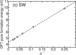
Figure 2: DFT pure formation energies of (a) MV, (b) SiS, and (c) SW defects in graphene against the reciprocal of the supercell size $N$. Fine ${\bf k}$-point grids were used in each supercell. Ultrasoft pseudopotentials were used. The dashed lines show fits of Eq. (5) to the data.

II.4 Backflow

DMC calculations in a $3\times 3$ supercell at a single twist for the MV show that the inclusion of backflow correlations with polynomial electron-electron and electron-nucleus terms lowers the pure defect formation energy by $41(30)$ meV, while the addition of the plane-wave electron-electron term further lowers the pure defect formation energy by $16(29)$ meV, giving a total lowering of $58(31)$ meV. These differences are statistically insignificant, and are an order of magnitude smaller than the error bars on the TA SJ-DMC pure defect formation energies reported in Table 2; fixed-node errors are therefore well controlled. A backflow function with electron-electron and electron-nucleus terms lowers the energy per atom of graphene by $46(9)$ meV, and the inclusion of the plane-wave electron-electron term does not have a statistically significant effect. Again, however, the effects of backflow are insignificant on the $0.1$ eV scale of the error bars on our SJ-DMC defect-formation energies.

III Results and discussion

III.1 Atomic structures

III.1.1 Pristine graphene, silicene, and bulk silicon

We have used a carbon-carbon bond length of 1.42 Å in all our pristine graphene calculations [61, 62], and we have used exactly the same supercell lattice parameters for our pristine and defective graphene calculations. For bulk silicon and silicene we used lattice parameters of $5.469$ and $3.866$ Å, respectively, obtained using DFT with the Perdew-Burke-Ernzerhof (PBE) exchange-correlation functional [58]. The sublattice buckling of silicene ($0.458$ Å) was also obtained by relaxing within DFT-PBE [49].

III.1.2 MV

It has previously been shown that a graphene MV undergoes a Jahn-Teller distortion, with two neighbors of the missing atom moving together to form a weak, reconstructed bond, and lowering the symmetry from $D_{3h}$ point group [14]. One DFT work on MVs has found and used a $C_{2v}$ structure (a planar structure with a single horizontal mirror plane and a single vertical mirror plane) [29]; other DFT works have found that when two neighbors of the missing atom form a reconstructed bond, the third neighbor moves out of plane [14, 80, 81], resulting in a structure of $C_{s}$ point group (a nonplanar structure with just a single vertical mirror plane).

As shown in Table 1, our non-spin-polarized DFT calculations in the local density approximation (LDA) and DFT-PBE calculations with and without many-body dispersion (MBD*) corrections [82, 83] find the $C_{s}$ MV structure to be favored (with the sole exception of DFT-LDA in a small, $3\times 3$ supercell). The energy differences between the different non-spin-polarized MV structures oscillate significantly with supercell size, but are less than $0.3$ eV. This is just about large enough to be non-negligible on the scale of our DMC error bars (see Sec. III.2). The difference between the $C_{s}$ DFT-PBE and DFT-PBE-MBD* structures is small. For example, in a $3\times 3$ supercell, the DFT-PBE energy is only increased by $1.5$ meV when the DFT-PBE-MBD* structure is used instead of the DFT-PBE structure. We have used the non-spin-polarized $C_{s}$-symmetry structures obtained by relaxing within DFT-PBE in our QMC calculations; the MV structure in a $5\times 5$ supercell is shown Fig. 3.

Table 1: DFT energies of the most stable $D_{3h}$, $C_{2v}$, and ${C_{s}}$ structures relative to the most stable non-spin-polarized ${C_{s}}$ structure. Different exchange-correlation functionals and supercell sizes are used. Spin-polarized and non-spin-polarized results are labelled by “(p)” and “(u)”, respectively. Ultrasoft pseudopotentials and fine ${\bf k}$-point grids are used.

		Energy relative to non-spin-polarized $C_{s}$ defect (meV)
Functional	Supercell	$E_{D_{3h}({\rm u})}-E_{C_{s}({\rm u})}$	$E_{C_{2v}({\rm u})}-E_{C_{s}({\rm u})}$	$E_{C_{2v}({\rm p})}-E_{C_{s}({\rm u})}$	$E_{C_{s}({\rm p})}-E_{C_{s}({\rm u})}$
LDA	$3\times 3$	$0$	$0$	$0$	$0$
LDA	$5\times 5$	$94.6$	$92.4$	$71.5$	$0$
LDA	$7\times 7$	$120.2$	$115.4$	$88.7$	$0$
PBE	$3\times 3$	$21.5$	$21.5$	$-36.4$	$-36.5$
PBE	$5\times 5$	$214.8$	$211.6$	$-96.8$	$-96.8$
PBE	$7\times 7$	$274.2$	$268.6$	$85.6$	$-113.8$
PBE-MBD*	$3\times 3$	$19.6$	$19.6$	$15.4$	$19.8$
PBE-MBD*	$5\times 5$	$195.6$	$193.7$	$-105.7$	$0$
PBE-MBD*	$7\times 7$	$245.9$	$250.8$	$-128.0$	$-122.3$

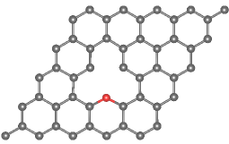
(a)

(b)

Figure 3: (a) Top-down and (b) in-plane views of the DFT-PBE-relaxed MV structure in a $5\times 5$ supercell. The undercoordinated carbon atom is shown in red.

Previous DFT calculations have found that the MV has a magnetic moment of $1.04\mu_{\text{B}}$–$2\mu_{\text{B}}$, where $\mu_{\text{B}}$ is the Bohr magneton [84, 85, 86]. We examine the effect of performing spin-polarized DFT calculations in Table 1. Within DFT-LDA, the MV is unambiguously nonmagnetic. Within DFT-PBE and DFT-PBE-MBD*, spin-polarized structures of $C_{2v}$ and $C_{s}$ symmetry are found to be stable. Convergence to the lowest-energy atomic structure is challenging in spin-polarized DFT calculations, where we often find structures with energies that are either greater than the non-spin-polarized energy for the same point group or greater than the energy of a higher-symmetry structure, demonstrating that we have not obtained the global minimum of the energy. To try to address this problem we have performed repeated spin-polarized calculations with different initial plane-wave coefficients and different initial geometries. Our DFT-PBE calculations in a $7\times 7$ supercell suggest that the spin-polarized $C_{s}$ MV structure is more stable than the non-spin-polarized $C_{s}$ structure by about $0.1$ eV, in agreement with previous DFT calculations [84], with magnetic moment $1.4\mu_{\text{B}}$. However, the energy differences between magnetic and nonmagnetic MV structures are less than or comparable to the error bars on our DMC defect-formation energies reported in Sec. III.2. Furthermore, there is no sign of convergence with respect to supercell size of the difference between the DFT energies of the magnetic and nonmagnetic structures. In a $3\times 3$ supercell, the DMC pure formation energy obtained using spin-polarized orbitals is within error bars of that obtained with non-spin-polarized orbitals. For consistency, we have used nonmagnetic MV structures and non-spin-polarized orbitals in our QMC calculations.

III.1.3 SiS

Replacing a single carbon atom by a silicon atom results in a defect of $C_{s}$ point group, rather than $D_{3h}$, due to a Jahn-Teller distortion [28]. The DFT-PBE-relaxed geometry shown in Fig. 4 has the silicon atom bonded with three carbon atoms and lying above the graphene plane due to partial $sp^{3}$ hybridization.

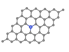
(a)

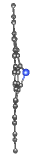
(b)

Figure 4: (a) Top-down and (b) in-plane views of the DFT-PBE-relaxed SiS structure in a $5\times 5$ supercell. The silicon atom is shown in blue.

III.1.4 SW defect

In graphene, a SW defect is formed by an in-plane rotation of a single carbon-carbon bond through $90^{\circ}$ about its midpoint. This transforms four hexagonal unit cells into two pentagons and two heptagons, as shown in Fig. LABEL:sub@subfig:sw1, with the same number of carbon atoms as pristine graphene and without any dangling bonds. The SW rotation compresses or stretches many bonds, resulting in a wave of significant vertical displacement of carbon atoms around the defect, as shown in Fig. LABEL:sub@subfig:sw2. The relaxed lattice will adopt either a “sine-like” buckled structure, in which the two rotated carbon atoms are slightly displaced in opposite out-of-plane directions, or a “cosine-like” buckled structure, in which the two rotated carbon atoms are slightly displaced in the same out-of-plane direction. The “sine-like” structure is the lower-energy configuration [87, 88], and is the structure studied in this work.

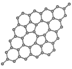
(a)

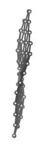
(b)

Figure 5: (a) Top-down and (b) in-plane views of the DFT-PBE-relaxed “sine-like” SW defect structure in a $5\times 5$ supercell.

III.2 Defect formation energies

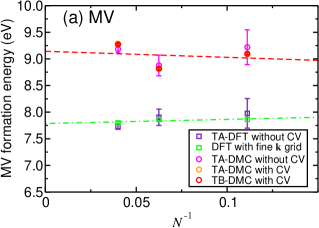
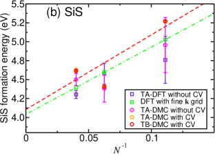
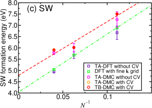
Figure 6: DFT and DMC formation energies against reciprocal of supercell size $N$, using different methods for dealing with momentum quantization errors, for (a) MV, (b) SiS, and (c) SW defects. The red dashed lines show an unweighted least-squares fit of Eq. (5) to the TA-DMC data. Both the DFT and DMC calculations used Dirac-Fock pseudopotentials. The carbon and silicon chemical potentials were taken to be the energy per atom of monolayer graphene and bulk silicon, extrapolated to infinite system size; hence the $N$-dependence shown in this figure only arises from the finite-concentration and finite-size effects in the pure formation energy.

Table 2: Theoretical static-nucleus formation energies for various point defects in monolayer graphene. The carbon and silicon chemical potentials are the energies per atom of graphene and bulk silicon, respectively. Results without citations were obtained in the present work. “NTBM” refers to a nonorthogonal tight-binding model. “DFT-B3LYP-D*” refers to DFT with a self-interaction-corrected hybrid B3LYP functional [89, 90]. To compare with experimental results, the vibrational free energies reported in Table 4 should be added to the static-nucleus data reported in this table.

Method	Defect formation energy (eV)
	MV	SiS	SW
DFT-PBE	$7.64$ [29], $7.65$ [34], $7.97$	$3.77$ [34], $6.85$ [91] $3.59$	$4.71$ [88], $4.32$
DFT-LDA	$8.02$ [29], $7.40$ [92], $8.25$		$4.66$ [93], $4.86$ [92], $5.42$ [88]
DFT-B3LYP-D*	$8.05$ [80]
NTBM			$4.60$ [36]
DMC			$5.82(3)$ [88]
DMC-corrected DFT	$9.0(1)$	$4.4(1)$	$4.9(1)$

Figure 6 shows DMC and DFT defect formation energies against system size. Twist averaging is either performed directly (without a CV), or by using the DFT results as a CV [i.e., fitting Eq. (4)]. Also shown are DFT results obtained with a fine ${\bf k}$-point mesh. The error bars on the “TA-DMC with CV” data were obtained using Gaussian propagation of errors through the fit of Eq. (4) to the DMC results at all 24 twists. The “TB-DMC” data were obtained using twist-blocking, in which six blocks of four twists were used to obtain a standard error estimate that includes both Monte Carlo random errors and finite-twist-sampling random errors. Figure 6 demonstrates that the use of a CV significantly reduces the random errors in the DMC energy data, and that subsequent twist-blocking to account for the remaining twist-sampling errors does not affect the random error estimate significantly (as we have also shown in Fig. 1). In theory, the most accurate way to obtain the TA energy is to fit Eq. (4) to formation energies in a single block of all the twists, and then to use TB to obtain the error bars, but the difference between the TA and TB mean energies is negligible in practice. However, the TB errors are not large enough to quantify the quasirandom finite-size errors in the formation energies at different supercell sizes; this finite-size noise must therefore arise from effects such as the enforced supercell commensurability of Ruderman-Kittel oscillations in the density and pair density rather than momentum quantization. Quasirandom finite-size effects are larger in the DMC formation energies than in the DFT results, presumably because of the explicit treatment of correlation in QMC methods. The obvious (but expensive) way to reduce this would be to perform DMC calculations in a larger range of supercell sizes and possibly shapes.

At each system size we evaluate a correction to the DFT formation energy as a difference between the TA-DMC result and the DFT result with a fine ${\bf k}$-point grid. The DMC corrections to the defect formation energies in different supercells (including the chemical potentials extrapolated to the thermodynamic limit) are given in Table 3. In general, the difference between the DFT and DMC formation energies is expected to be dominated by short-range effects, with systematic finite-concentration errors (due to electrostatic and elastic effects) being similar in DFT and DMC; this is confirmed by the similar gradients of the fitted lines in Fig. 6. However, the difference between DFT and DMC shows quasirandom fluctuations as a function of system size. This suggests that the best scheme for using DMC to evaluate defect formation energies is to average the difference between TA-DMC and fine-${\bf k}$-point DFT formation energies obtained in multiple supercells, and then to apply the resulting correction to DFT results extrapolated to the dilute limit of infinite supercell size. Averaging over multiple supercells is clearly necessary, because the difference between DMC and DFT results obtained in different cell sizes in Table 3 fluctuates randomly by an amount that is significantly larger than the error bars on the individual differences. DFT-PBE significantly underestimates the formation energy for all three defects. The larger DMC correction for the MV formation energy compared to the SiS and SW defects reported in Table 3 suggests that DFT performs relatively poorly when evaluating energy differences between structures with very different chemical bonding.

Table 3: Difference between DMC and DFT-PBE static-nucleus formation energies for various defects, evaluated as the difference between defect-formation energies calculated with TA-DMC [using Eq. (4)] and DFT-PBE using a fine ${\bf k}$-point grid. The DFT calculations use ultra-soft pseudopotentials rather than the Trail-Needs Dirac-Fock pseudopotentials used by the QMC calculations.

Supercell	DMC correction to formation energy (eV)
	MV	SiS	SW
$3\times 3$	$1.09(3)$	$1.07(9)$	$0.65(2)$
$4\times 4$	$0.78(3)$	$0.54(9)$	$0.27(2)$
$5\times 5$	$1.28(2)$	$0.91(9)$	$0.70(3)$
Mean	$\!\!\!1.1(1)$	$\!\!\!0.8(1)$	$\!\!\!0.5(1)$

Our final DFT and DMC defect formation energies are shown in Table 2, along with DFT results from the literature. The DMC literature result for the SW formation energy [88], which has a comparatively tiny standard error, was only calculated in a $5\times 5$ supercell with no attempt to control finite-size effects; our standard error is larger because it accounts for quasirandom finite-size effects.

The DFT-PBE differences in the zero-point vibrational energies and Helmholtz free energies at $298$ K between defective and pristine graphene for the MV, SiS, and SW defects are shown in Table 4. These vibrational free energy contributions should be added to the static-nucleus defect formation energies in Table 2. The vibrationally corrected DMC defect formation energies are $8.3(1)$, $3.6(1)$, and $4.4(1)$ at $298$ K for MV, SiS, and SW defects, respectively. The vibrationally corrected DMC MV formation energy may be compared with an experimentally determined MV formation energy, $7.0(5)$ eV [94]. While the difference between this experimental result and our result is statistically significant, it should be noted that the uncertainty in the experimental result is fairly large. Furthermore, there are some systematic errors that affect our DMC result, such as the use of DFT-relaxed geometries and estimating the Helmholtz free energy using the harmonic approximation.

Table 4: DFT-PBE vibrational contributions to the Helmholtz free energies of formation of various point defects in monolayer graphene. The contributions are extrapolated to the dilute limit.

Temperature (K)	Vib. contrib. to form. energy (eV)
	MV	SiS	SW
0	$-0.74$	$-0.44$	$-0.49$
298	$-0.68$	$-0.41$	$-0.47$

III.3 Atomization energies

DMC atomization energies are plotted against system size in Fig. 7 for graphene, bulk silicon, and silicene, respectively, showing that finite-size effects are largely removed by extrapolation. DFT-PBE vibrational Helmholtz free energies are reported in Table 5. In graphene the vibrational free energy is relatively small, due to the extreme stiffness of the lattice. At room temperature, vibrational effects stabilize silicene with respect to bulk diamond-structure silicon.

Table 5: DFT-PBE vibrational Helmholtz free energies per atom for pristine graphene, bulk silicon, and silicene.

Temperature (K)	Vibrational free energy (meV/atom)
	Graphene	Silicon	Silicene
0	$3.0$	$61.9$	$50.6$
298	$3.2$	$36.1$	$3.0$

Figure 7: TA-DMC static-nucleus atomization energies of (a) graphene, (b) bulk silicon, and (c) silicene against $N^{-5/4}$ for graphene and silicene, and $N^{-1}$ for bulk silicon, where $N$ is the number of primitive cells in the supercell. The atomization energies are defined with respect to the DMC spin-polarized ${}^{3}\text{P}_{0}$ ground states of isolated carbon and silicon atoms.

Table 6: Helmholtz free energies of atomization of graphene, bulk silicon, and silicene. The DFT-PBE vibrational free-energies shown in Table 5 have been subtracted from our static-nucleus atomization energies. Unlike the present work, the silicene DFT calculations in Refs. 45 and 49 used a non-spin-polarized (¹S₀) Si atom as the atomic reference state, obtaining DFT-LDA atomization energies of $5.06$ [45] and $5.12$ eV [49] and DFT-PBE and DFT-HSE06 atomization energies of $4.69$ and $4.70$ eV, respectively [49]. The difference between the single-determinant DMC energies of a non-spin-polarized (¹S₀) and a spin-polarized (${}^{3}\text{P}_{0}$) silicon atom is $1.1506(6)$ eV. The difference is $0.6107$ eV within DFT-LDA and $0.7987$ eV within DFT-PBE. The atomic reference state for the graphene atomization energies is the spin-polarized (${}^{3}\text{P}_{0}$) ground state of an isolated carbon atom. Results without citations were obtained in the present work.

Method	Atomization energies (eV/atom)
	Graphene		Bulk silicon		Silicene
Temperature	$0$ K	$298$ K	$0$ K	$298$ K	$0$ K	$298$ K
DFT-LDA	$8.96$ [95], $8.632$ [96], $8.912$	$8.912$	$5.34$ [97], $5.3$ [98], $5.29$	$5.31$	$4.5414$	$4.5869$
DFT-PW91			$4.653$ [97]
DFT-PBE	$7.93$ [95], $7.873$ [96], $7.916$	$7.915$	$4.55$	$4.58$	$3.9238$	$3.9714$
GFMC			$4.51(3)$ [98]
DMC	$7.395(3)$ [96], $7.388(2)$	$7.388(2)$	$4.62(1)$ [97], $4.63(2)$ [99], $4.4815(6)$	$4.5073(6)$	$3.7075(4)$	$3.7551(4)$
Experiment	$7.357(5)$ [100]		$4.62(8)$ [101, 102]

Vibrationally corrected DMC atomization energies for free-standing graphene, bulk silicon, and free-standing silicene, extrapolated to infinite system size, are reported in Table 6, along with DFT results. The atomization energies of both bulk silicon and silicene are significantly overestimated in DFT compared with DMC. Bulk silicon is energetically more stable than silicene by a huge margin of $0.7522(5)$ eV/atom. By contrast, the atomization energies of graphite, graphene, and carbon diamond are very similar, at about $7.43$ eV/atom [103, 96]. Our DMC result for graphene compares extremely well with the experimental result for graphite [100], the two differing by only $\sim 0.02$ eV/atom. For the atomization energy of bulk silicon there is a small but statistically significant difference between our DMC result and earlier works [97, 99]; this is probably due to the fact that the earlier works did not use twist averaging. The DMC and DFT-PBE results are in reasonable agreement with the experimentally determined atomization energy of bulk silicon.

IV Conclusions

We have used QMC methods to investigate the accuracy of DFT in first-principles studies of point defect formation in monolayer graphene. Over accessible ranges of supercell size ($3\times 3$–$5\times 5$ primitive cells), both DFT and QMC formation energies are affected by both systematic and quasirandom finite-concentration effects on a $\sim 1$ eV energy scale. Systematic finite-concentration effects are similar in QMC and DFT, but the difference between the QMC and DFT formation energies is still subject to quasirandom errors, of order $0.5$ eV. To reduce these errors, the difference between QMC and DFT formation energies may be averaged over supercell sizes, providing a correction that can be applied to the DFT formation energy obtained using large supercell sizes. We find that DFT-PBE underestimates the formation energies of isolated monovacancies, silicon substitutions, and Stone-Wales defects by a significant margin of order 1 eV. Vibrational contributions to the free energies of formation of point defects in graphene have also been found to be non-negligible, on a 0.5–1 eV energy scale. Thus there are many factors to balance when evaluating defect formation energies in 2D materials from first principles. Similarly challenging behavior is expected for related quantities such as defect migration energy barriers.

We have also compared the QMC atomization energies of monolayer graphene, silicene, and bulk silicon, finding that bulk silicon is more stable than silicene by $0.7522(5)$ eV per atom. This quantifies the significant thermodynamic challenge involved in producing free-standing silicene.

Appendix A Computational details

A.1 DFT calculations

A.1.1 Total energy, geometry optimization, and phonon calculations

Our DFT calculations were performed using the PBE generalized gradient approximation exchange-correlation functional [58] and the plane-wave-basis code castep [59]. The total energy, geometry optimization, and phonon calculations all used ultrasoft pseudopotentials [60] to represent the nuclei and core electrons. A plane-wave cutoff energy of $556$ eV was used for pristine and defective graphene and a cutoff energy of $305$ eV was used for bulk silicon and silicene. For pristine graphene and silicene, the total energies were calculated using $51\times 51$ and $53\times 53$ Monkhorst-Pack ${\bf k}$-point grids, respectively. The total energies of defective graphene were calculated for supercells of $N$ primitive cells in a $\sqrt{N}\times\sqrt{N}$ arrangement containing a single defect, using Monkhorst-Pack grids of approximately $(51/\sqrt{N})\times(51/\sqrt{N})$ ${\bf k}$-points; in the following we refer to the use of these grids as “fine” ${\bf k}$-point sampling. The geometry in each of the defective graphene supercells was optimized to a force tolerance of $0.0025$ eV Å^-1 with fixed lattice vectors corresponding to a pristine-graphene carbon-carbon bond length of $1.42$ Å [61, 62]. Our bulk silicon calculations used $17\times 17\times 17$ Monkhorst-Pack ${\bf k}$-point grids. All our 2D DFT calculations were performed using an artificial periodicity of 30 bohr in the out-of-plane direction. Non-spin-polarized calculations were used except where stated otherwise.

Phonon calculations using the finite displacement method in DFT were used to evaluate the vibrational contributions to the free energy. These calculations were performed using atomic displacements of $0.005$, $0.01$, $0.015$, $0.02$, and $0.025$ bohr, with the final energies obtained by linearly extrapolating to zero atomic displacement. For each supercell $5\times 5$ Monkhorst-Pack supercell ${\bf k}$-point grids were used. Geometries were first optimized to a force tolerance of $0.0005$ eV Å^-1.

A.1.2 QMC orbital generation

Our DFT orbital-generation calculations used the PBE functional together with Trail-Needs Dirac-Fock pseudopotentials [63, 64] to represent the nuclei and core electrons, with $s$ being the angular momentum of the local component when the pseudopotentials are re-represented in Kleinman-Bylander form [65]. The geometry was fixed at the DFT-PBE geometry obtained using ultrasoft pseudopotentials. The graphene supercells used for the QMC calculations consisted of $3\times 3$, $4\times 4$, and $5\times 5$ primitive cells, where the plane-wave cutoff energy for the smaller two supercells was $3401$ eV, and the plane-wave cutoff energy for the larger supercell was $2231$ eV. These cutoff energies are such that the DFT energy per atom is converged to within, respectively, $0.1$ mHa and $1.59$ mHa (known as chemical accuracy) [66]. For bulk silicon, supercells of $2\times 2\times 2$, $3\times 3\times 3$, and $4\times 4\times 4$ primitive cells were used with a plane-wave cutoff energy of $2231$ eV for all system sizes, while the silicene supercells comprised $3\times 3$ and $6\times 6$ arrays of primitive cells. An artificial periodicity of $30$ bohr was used for the graphene and silicene calculations. Non-spin-polarized DFT calculations were used except where otherwise stated.

A.2 QMC calculations

A.2.1 Trial wave functions

The trial wave functions used for the QMC calculations were of Slater-Jastrow (SJ) form, containing a product of determinants of spin-up and spin-down orbitals; see Sec. A.1.2. Different sets of orbitals were generated for each twist (i.e., offset ${\bf k}_{\text{s}}$ to the grid of Bloch ${\bf k}$ vectors). The plane-wave orbitals were re-represented in a blip (B-spline) basis [67] both for computational efficiency in the QMC calculations and to remove the unwanted periodicity in the out-of-plane direction. The Jastrow factor, a nodeless function of the interparticle distances containing optimizable free parameters, consisted of polynomial electron-electron, electron-nucleus, and electron-electron-nucleus terms, and plane-wave electron-electron terms [68]. Trial wave functions were optimized first by minimizing the variance of the energy [69, 70] and then by minimizing the energy expectation value [71]. For a given supercell, this optimization was performed at a single, randomly chosen twist, with the resulting Jastrow factor being used at all twists.

For some test cases at individual twists, Slater-Jastrow-backflow trial wave functions were used to investigate the fixed-node errors in our SJ-DMC results. These wave functions were obtained by optimizing the backflow and Jastrow parameters together using energy minimization. The backflow functions contained polynomial electron-electron and electron-nucleus terms [72]. Further tests using a long-range plane-wave electron-electron backflow function were also carried out: see Sec. II.4.

Trail-Needs Dirac-Fock pseudopotentials [63, 64] were used to represent the ionic cores, with $d$ being the angular momentum of the local component.

A.2.2 DMC calculations

To calculate the pure defect formation energy of each of the three defects we have studied in graphene, pairs of DMC calculations were carried out at each twist in all the defective and pristine graphene supercells. Time steps of $\tau=0.04$ and $0.16$ Ha^-1 were used in these calculations, with the corresponding target walker populations being varied in inverse proportion to the time step. In all cases the target population was at least 256 walkers. The energies were then extrapolated linearly to zero time step. For the total energies of defective and pristine graphene we would not expect these time steps to be small enough to be in the linear bias regime (as confirmed by the results shown in Fig. 8); however, as shown in Fig. 9, the nonlinear parts of the time-step bias largely cancel out of the pure defect formation energy.

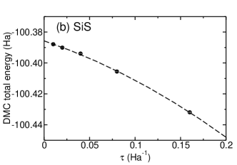
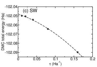
Figure 8: DMC total energies per supercell of (a) MV, (b) SiS, and (c) SW defects in a $3\times 3$ supercell of graphene against DMC time step $\tau$ at a single, randomly chosen twist $\mathbf{k}_{\text{s}}$. The dashed lines show quadratic fits to the energy as a function of time step.

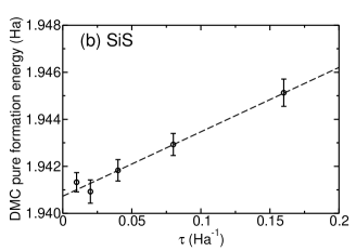
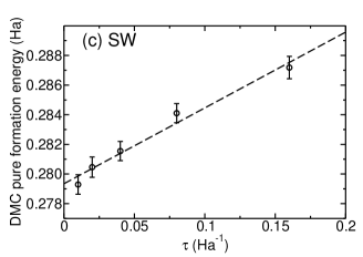
Figure 9: DMC pure formation energies of (a) MV, (b) SiS, and (c) SW defects in a $3\times 3$ supercell of graphene against DMC time step $\tau$ at the twist $\mathbf{k}_{\text{s}}$ used in Fig. 8. The dashed lines show linear fits to the pure formation energy as a function of time step.

To calculate the energies per atom of graphene and bulk silicon we used smaller time steps of $\tau=0.01$ and $0.04$ Ha^-1, allowing time-step bias in the total energy per atom to be largely removed by linear extrapolation. Again, we varied the target walker population inversely with time step.