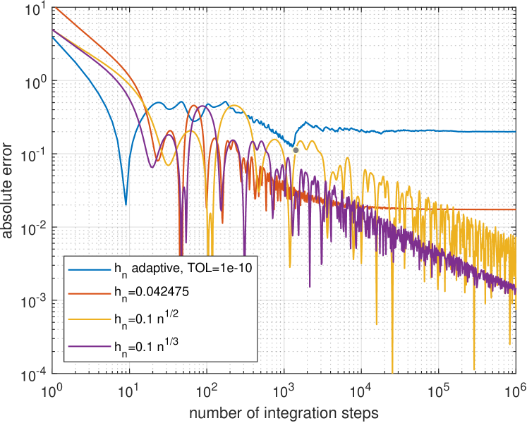
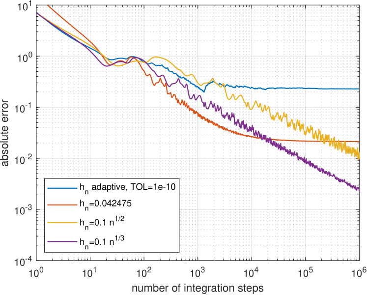
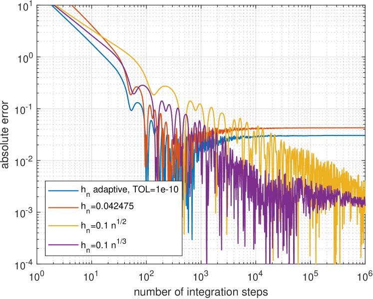
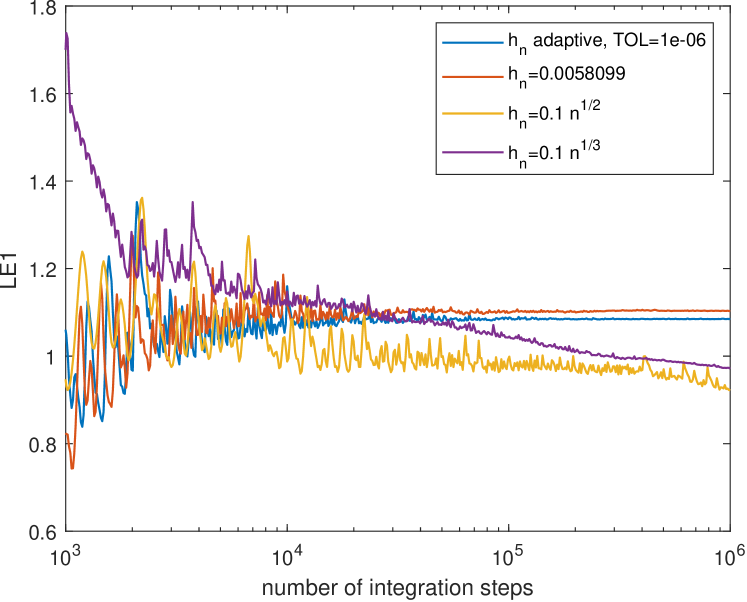
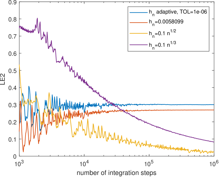
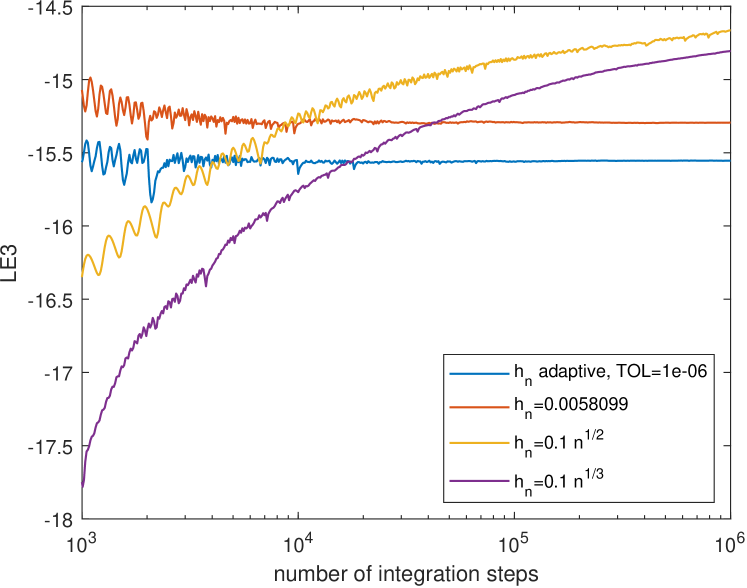
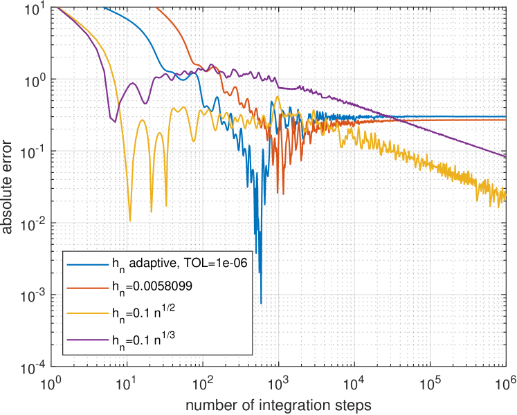
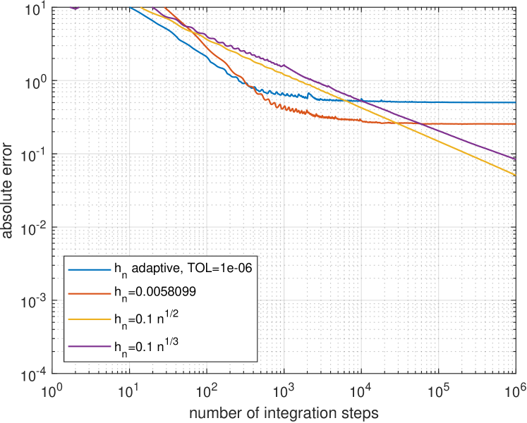
\NewEnviron

scaletikzpicturetowidth[1]\BODY \DeclareSourcemap \maps[datatype=bibtex] \map \pernottypemisc \step[fieldset=url, null] \step[fieldset=urldate, null] \DeclareRedundantLanguages English, english, german, french, eng english, german, ngerman, french

Stepsize Variations for Lyapunov Exponents to Counter Persistent Errors

Florian Noethen Fachbereich Mathematik, Universität Hamburg, Bundesstraße 55, 20146 Hamburg, Germany (florian.noethen@uni-hamburg.de, ORCID 0000-0001-9609-8206).
(March 6, 2024)
Abstract

Lyapunov exponents are important quantities in the analysis of complex dynamical systems. Usually, they are computed with Benettin’s algorithm, which propagates linear perturbations along a background trajectory. While many applications trust in convergence of the algorithm, they often do not consider the effects of numerical errors. In fact, numerical errors tend to accumulate in the averaging process of Benettin’s algorithm when using constant or adaptive stepsizes and lead to limits different from the Lyapunov exponents.

In this article, we demonstrate how local integration errors can affect the convergence of Benettin’s algorithm and suggest rules for stepsizes to counter persistent errors. Our examples demonstrate that stepsize variations can improve the accuracy of Benettin’s algorithm. More rigorous results are obtained in a theoretical analysis, in which we prove convergence of Benettin’s algorithm for linear systems.

Keywords: Lyapunov exponents; Benettin’s algorithm; stepsize variations; linear dynamical systems; convergence analysis

1 Introduction

Lyapunov exponents, named after the Russian mathematician Aleksandr Mikhailovich Lyapunov, are important quantities in the analysis of complex dynamical systems. They describe asymptotic rates at which linear perturbations to solutions of dynamical systems grow (or decay). Hence, Lyapunov exponents can be used to investigate stability properties of aperiodic motion, assuming regularity111The necessity of the regularity assumption was highlighted by Perron, who constructed an example in which a trajectory is Lyapunov unstable but its first approximation only has negative Lyapunov exponents [17]., and thereby generalize the classical stability theory of steady states and periodic orbits [18].

Next to stability theory, Lyapunov exponents can be applied to measure the complexity of attracting sets via the Lyapunov or Kaplan-Yorke dimension, which is a fractal dimension and gives an upper bound to the correlation dimension [13]. Moreover, the inverse of the largest Lyapunov exponent can be understood as a timescale for chaotic motion that indicates how long we may trust numerical predictions of a model. Another application involves the detection of Lagrangian coherent structures via finite-size or finite-time versions of the Lyapunov exponents [28, 15].

Although Lyapunov exponents are a frequent tool in numerical studies of chaotic systems, the most common algorithm to compute them has persisted since almost half a century. The underlying idea is to propagate a set of perturbations in the linearized model along a given background trajectory, while the propagated vectors are reorthonormalized periodically. The Lyapunov exponents are then computed as averages of volume expansion (or contraction) via the rescaling factors from the orthonormalization procedure [5, 6, 29]. We refer to this method as Benettin’s algorithm. The propagated vectors can be used further to compute the so-called covariant Lyapunov vectors, which are natural directions corresponding to the Lyapunov exponents [12, 31, 16].

While convergence of Benettin’s algorithm and of algorithms for covariant Lyapunov vectors have been proved analytically222In the absence of numerical errors, convergence of Benettin’s algorithm is a direct consequence of the multiplicative ergodic theorem and its version for exterior powers [2], whereas convergence of algorithms for covariant Lyapunov vectors require a more in-depth analysis [24, 25]., the effects of numerical errors are still not fully understood. There are various error sources in both the nonlinear and the linearized systems. As we will see in this article, even in the absence of errors from the nonlinear system, integration errors from the linearized system can accumulate and influence the computation of Lyapunov exponents. In particular, if the stepsizes are constant, the output of Benettin’s algorithm usually does not converge to the exact Lyapunov exponents due to persistent errors. In practice, there is often no way of quantifying these errors, since the exact Lyapunov exponents are usually unknown due to the complex nature of the dynamical systems for which they are considered. Thus, errors in the computation of Lyapunov exponents for nonlinear systems are seldom mentioned, let alone quantified.

Major efforts have been made for linear systems by Luca Dieci, Erik S. Van Vleck and co-authors. They advocate the use of adaptive stepsizes to bound the local integration error and were able to prove error estimates for computed Lyapunov exponents of linear systems that are regular and have stable Lyapunov exponents [9, 10]. Implementations for linear and nonlinear systems are presented in [8, 7]. While Dieci and Van Vleck prove that Lyapunov exponents can be approximated arbitrarily close in the limit by decreasing the error tolerance or stepsize, there is no true convergence. Each time a better approximation is sought, the tolerance or stepsize has to be decreased and the algorithm has to be rerun from the beginning for a longer time. Instead, true convergence requires to simultaneously decrease the integration time and stepsize, as it was already conjectured by Mc Donald and Higham in their error analysis for autonomous linear systems in 2001 [21, Sec. 5].

In this article, we follow Mc Donald’s and Higham’s suggestion and introduce stepsize variations that tackle both limits simultaneously. We provide conditions for stepsizes under which Benettin’s algorithm convergences to the true Lyapunov exponents. Our convergence result requires regularity and fast-invertibility, which is a weaker assumption than stability of Lyapunov exponents, and even holds for degenerate Lyapunov spectra.

Theorem (Convergence of Benettin’s algorithm)

Assume a linear dynamical system with bounded growth that is regular and fast-invertible. If the numerical solver is consistent of order p>0𝑝0p>0 and if the stepsizes hnsubscript𝑛h_{n} fulfill

n=1hn=andn=1hnp+1<,formulae-sequencesuperscriptsubscript𝑛1subscript𝑛andsuperscriptsubscript𝑛1superscriptsubscript𝑛𝑝1\sum_{n=1}^{\infty}h_{n}=\infty\hskip 10.00002pt\text{and}\hskip 10.00002pt\sum_{n=1}^{\infty}h_{n}^{p+1}<\infty,

then Benettin’s algorithm converges in the presence of integration errors.

The article is structured as follows: We first provide a theoretical foundation for Lyapunov exponents of linear systems (Section 2) before presenting Benettin’s algorithm (Section 3). Afterwards, we derive conditions for varying stepsizes under which to expect convergence and prove a precise version of the above theorem (Section 4). Our new approach is compared to the usual adaptive or constant stepsizes in three numerical examples (Section 5). Finally, we conclude our findings (Section 6).


2 Theory of Lyapunov exponents

In this section, we define Lyapunov exponents and present some of their properties. We mainly follow the book by Adrianova [1], which provides a well-written introduction to characteristic exponents for linear systems, and the book by Arnold [2], which contains various versions of the multiplicative ergodic theorem in the context of random dynamical systems.

We focus on one-sided dynamical systems arising from linear differential equations. More abstractly, we assume a map X(t,s)𝑋𝑡𝑠X(t,s) describing the propagation of vectors from time s𝑠s to time t𝑡t with the following properties:

  • XC1(0×0,d×d)𝑋superscript𝐶1subscriptabsent0subscriptabsent0superscript𝑑𝑑X\in C^{1}(\mathbb{R}_{\geq 0}\times\mathbb{R}_{\geq 0},\mathbb{R}^{d\times d}),

  • X(t,t)=I𝑋𝑡𝑡𝐼X(t,t)=I for all t0𝑡0t\geq 0, and

  • X(t,s)=X(t,h)X(h,s)𝑋𝑡𝑠𝑋𝑡𝑋𝑠X(t,s)=X(t,h)X(h,s) for all s,t,h0𝑠𝑡0s,t,h\geq 0.

It follows that X1(t,s)=X(s,t)superscript𝑋1𝑡𝑠𝑋𝑠𝑡X^{-1}(t,s)=X(s,t). In particular, X(t):=X(t,0)assign𝑋𝑡𝑋𝑡0X(t):=X(t,0) is the fundamental matrix of the linear differential equation x˙=A(t)x˙𝑥𝐴𝑡𝑥\dot{x}=A(t)x with A(t0):=d/dt|t=t0X(t,t0)assign𝐴subscript𝑡0evaluated-at𝑑𝑑𝑡𝑡subscript𝑡0𝑋𝑡subscript𝑡0A(t_{0}):=d/dt|_{t=t_{0}}X(t,t_{0}), and X(t,s)=X(t)X1(s)𝑋𝑡𝑠𝑋𝑡superscript𝑋1𝑠X(t,s)=X(t)X^{-1}(s).

Let us further assume that the dynamical system has bounded growth, i.e., there exists MX>0subscript𝑀𝑋0M_{X}>0 such that

veMX|ts|X(t,s)vveMX|ts|norm𝑣superscript𝑒subscript𝑀𝑋𝑡𝑠norm𝑋𝑡𝑠𝑣norm𝑣superscript𝑒subscript𝑀𝑋𝑡𝑠\|v\|e^{-M_{X}|t-s|}\leq\|X(t,s)v\|\leq\|v\|e^{M_{X}|t-s|}

for all s,t0𝑠𝑡0s,t\geq 0 and all vd𝑣superscript𝑑v\in\mathbb{R}^{d}. In view of the underlying equation, the bounded growth follows from suptA(t)MXsubscriptsupremum𝑡norm𝐴𝑡subscript𝑀𝑋\sup_{t}\|A(t)\|\leq M_{X}. Here, .=.2\|.\|=\|.\|_{2} denotes the spectral norm. Any norm different from the spectral norm will be marked accordingly.

2.1 Characteristic exponents

In this subsection, we define characteristic exponents and Lyapunov exponents.

Definition 2.1 ([1, Def. 2.1.1])

The characteristic exponent of f:[t0,):𝑓subscript𝑡0f:[t_{0},\infty)\to\mathbb{R} is given by

χ[f]:=lim supt1tlog|f(t)|{±}.assign𝜒delimited-[]𝑓subscriptlimit-supremum𝑡1𝑡𝑓𝑡plus-or-minus\chi[f]:=\limsup_{t\to\infty}\frac{1}{t}\log|f(t)|\in\mathbb{R}\cup\{\pm\infty\}.

A few handy properties follow easily from the definition [1, p. 26],[2, Lemma 3.2.1]:

  1. 1.

    χ[c]=0𝜒delimited-[]𝑐0\chi[c]=0 for all const. c0𝑐0c\neq 0

  2. 2.

    χ[cf]=χ[f]𝜒delimited-[]𝑐𝑓𝜒delimited-[]𝑓\chi[cf]=\chi[f] for all const. c0𝑐0c\neq 0,

  3. 3.

    χ[f]χ[g]𝜒delimited-[]𝑓𝜒delimited-[]𝑔\chi[f]\leq\chi[g] if |f||g|𝑓𝑔|f|\leq|g|,

  4. 4.

    χ[f+g]max(χ[f],χ[g])𝜒delimited-[]𝑓𝑔𝜒delimited-[]𝑓𝜒delimited-[]𝑔\chi[f+g]\leq\max(\chi[f],\chi[g]) with equality if χ[f]χ[g]𝜒delimited-[]𝑓𝜒delimited-[]𝑔\chi[f]\neq\chi[g],

  5. 5.

    χ[fg]χ[f]+χ[g]𝜒delimited-[]𝑓𝑔𝜒delimited-[]𝑓𝜒delimited-[]𝑔\chi[fg]\leq\chi[f]+\chi[g] (if the right-hand side makes sense).

In the context of dynamical systems, the characteristic exponent can be used to measure the (upper) exponential growth of a solution333When the underlying dynamical system is clear, we speak of characteristic exponents of (initial) vectors instead of characteristic exponents of the norms of their corresponding solutions.

χ[v]:=χ[X(t)v]=lim supt1tlogX(t)v,assign𝜒delimited-[]𝑣𝜒delimited-[]norm𝑋𝑡𝑣subscriptlimit-supremum𝑡1𝑡norm𝑋𝑡𝑣\chi[v]:=\chi[\|X(t)v\|]=\limsup_{t\to\infty}\frac{1}{t}\log\|X(t)v\|, (1)

where vd{0}𝑣superscript𝑑0v\in\mathbb{R}^{d}\setminus\{0\} is the initial vector. Since vectors with distinct characteristic exponents are linearly independent, the characteristic exponents can take at most d𝑑d values

>MXλ1>>λpMX>.subscript𝑀𝑋subscript𝜆1subscript𝜆𝑝subscript𝑀𝑋\infty>M_{X}\geq\lambda_{1}>\dots>\lambda_{p}\geq-M_{X}>-\infty.

In particular, there is a filtration of subspaces

d=V1V2VpVp+1:={0}superscript𝑑subscript𝑉1superset-ofsubscript𝑉2superset-ofsuperset-ofsubscript𝑉𝑝superset-ofsubscript𝑉𝑝1assign0\mathbb{R}^{d}=V_{1}\supset V_{2}\supset\dots\supset V_{p}\supset V_{p+1}:=\{0\} (2)

with Vi:={v:χ[v]λi}assignsubscript𝑉𝑖conditional-set𝑣𝜒delimited-[]𝑣subscript𝜆𝑖V_{i}:=\{v\,:\,\chi[v]\leq\lambda_{i}\} for i=1,,p𝑖1𝑝i=1,\dots,p such that

χ[v]=λivViVi+1.formulae-sequence𝜒delimited-[]𝑣subscript𝜆𝑖iff𝑣subscript𝑉𝑖subscript𝑉𝑖1\chi[v]=\lambda_{i}\hskip 10.00002pt\iff\hskip 10.00002ptv\in V_{i}\setminus V_{i+1}.

We set di:=dimVidimVi+1assignsubscript𝑑𝑖dimensionsubscript𝑉𝑖dimensionsubscript𝑉𝑖1d_{i}:=\dim V_{i}-\dim V_{i+1}.

Definition 2.2

The (forward) Lyapunov spectrum (λi,di)i=1,,psubscriptsubscript𝜆𝑖subscript𝑑𝑖𝑖1𝑝(\lambda_{i},d_{i})_{i=1,\dots,p} of a system consists of its Lyapunov exponents λisubscript𝜆𝑖\lambda_{i} together with their multiplicities disubscript𝑑𝑖d_{i}. A Lyapunov exponent λisubscript𝜆𝑖\lambda_{i} is called simple or nondegenerate if di=1subscript𝑑𝑖1d_{i}=1 and otherwise degenerate. If all Lyapunov exponents are simple, we call the Lyapunov spectrum simple.

While there are results indicating that simple Lyapunov spectra are generic [3, 22, 23], higher multiplicities may be forces by symmetries of the underlying system. Hence, we also consider degenerate spectra.

2.2 Regularity

In view of numerical computations, it is easier to work with limits instead of limes superiors. To this end, we introduce the concept of regularity and present its implications for singular values and vectors of the fundamental matrix.

Definition 2.3 ([2, p. 115])

We call a system (forward) regular444The definition from Arnold’s book is equivalent to [1, Def. 3.5.1]. This can be checked via [1, Lemma 3.5.1] and the Liouville-Ostrogradski formula detX(t)=detX(t0)et0ttr(A(τ))𝑑τ.𝑋𝑡𝑋subscript𝑡0superscript𝑒superscriptsubscriptsubscript𝑡0𝑡tr𝐴𝜏differential-d𝜏\det X(t)=\det X(t_{0})e^{\int_{t_{0}}^{t}\textnormal{tr}(A(\tau))\,d\tau}. if

i=1pdiλi=lim inft1tlog|detX(t)|.superscriptsubscript𝑖1𝑝subscript𝑑𝑖subscript𝜆𝑖subscriptlimit-infimum𝑡1𝑡𝑋𝑡\sum_{i=1}^{p}d_{i}\lambda_{i}=\liminf_{t\to\infty}\frac{1}{t}\log|\det X(t)|.

Regular systems are well-behaved in the sense that nonlinear perturbations of the underlying linear equations retain stability properties [2, p. 115]. Moreover, regular systems have sharp characteristic exponents.

Lemma 2.4 ([1, Thm. 3.9.1])

Regular systems have sharp characteristic exponents, i.e., it holds

χ[v]=limt1tlogX(t)v.𝜒delimited-[]𝑣subscript𝑡1𝑡norm𝑋𝑡𝑣\chi[v]=\lim_{t\to\infty}\frac{1}{t}\log\|X(t)v\|.
Corollary 2.5

The largest Lyapunov exponent of a regular system can be obtained as

λ1=limt1tlogσ1(X(t)),subscript𝜆1subscript𝑡1𝑡subscript𝜎1𝑋𝑡\lambda_{1}=\lim_{t\to\infty}\frac{1}{t}\log\sigma_{1}(X(t)),

where σ1subscript𝜎1\sigma_{1} denotes the largest singular value.

Proof.

Let e1,,edsubscript𝑒1subscript𝑒𝑑e_{1},\dots,e_{d} be the standard basis of dsuperscript𝑑\mathbb{R}^{d} and fix j𝑗j with ejV2subscript𝑒𝑗subscript𝑉2e_{j}\notin V_{2}. Since σ1(X(t))=X(t)subscript𝜎1𝑋𝑡norm𝑋𝑡\sigma_{1}(X(t))=\|X(t)\|, the claim follows from

X(t)ejX(t)dmaxiX(t)ei.norm𝑋𝑡subscript𝑒𝑗norm𝑋𝑡𝑑subscript𝑖norm𝑋𝑡subscript𝑒𝑖\|X(t)e_{j}\|\leq\|X(t)\|\leq\sqrt{d}\max_{i}\|X(t)e_{i}\|.

In subsection Subsection 2.4, we show that regularity of X𝑋X implies regularity of its exterior powers. In particular, it follows that all singular values of X(t)𝑋𝑡X(t) have sharp characteristic exponents.

Proposition 2.6

If X𝑋X is regular, then

Λi=limt1tlogσi(X(t))subscriptΛ𝑖subscript𝑡1𝑡subscript𝜎𝑖𝑋𝑡\Lambda_{i}=\lim_{t\to\infty}\frac{1}{t}\log\sigma_{i}(X(t))

for all i=1,,d𝑖1𝑑i=1,\dots,d, where σ1(X(t))σd(X(t))subscript𝜎1𝑋𝑡subscript𝜎𝑑𝑋𝑡\sigma_{1}(X(t))\geq\dots\geq\sigma_{d}(X(t)) denote the singular values of X(t)𝑋𝑡X(t) and Λ1,,ΛdsubscriptΛ1subscriptΛ𝑑\Lambda_{1},\dots,\Lambda_{d} denote the Lyapunov exponents counted according to their multiplicities555Given a Lyapunov spectrum (λi,di)i=1,,psubscriptsubscript𝜆𝑖subscript𝑑𝑖𝑖1𝑝(\lambda_{i},d_{i})_{i=1,\dots,p} we set Λ1,,Λd1=λ1,,Λd1++dp1+1,,Λd=λp.absentsubscript𝜆1subscriptΛ1subscriptΛsubscript𝑑1absentsubscript𝜆𝑝subscriptΛsubscript𝑑1subscript𝑑𝑝11subscriptΛ𝑑\underset{=\lambda_{1}}{\underbrace{\Lambda_{1},\dots,\Lambda_{d_{1}}}},\dots,\underset{=\lambda_{p}}{\underbrace{\Lambda_{d_{1}+\dots+d_{p-1}+1},\dots,\Lambda_{d}}}. .

We prove Proposition 2.6 in Subsection 2.4. Next, let us state a result on singular vectors of X(t)𝑋𝑡X(t).

Proposition 2.7

If X𝑋X is regular and u1(t),,ud(t)subscript𝑢1𝑡subscript𝑢𝑑𝑡u_{1}(t),\dots,u_{d}(t) denote the right singular vectors of X(t)𝑋𝑡X(t), then Ui(t)subscript𝑈𝑖𝑡U_{i}(t) given by span(ud1++di1+1(t),,ud1++di(t)))\textnormal{span}(u_{d_{1}+\dots+d_{i-1}+1}(t),\dots,u_{d_{1}+\dots+d_{i}}(t))) converges to Ui:=Vi+1Viassignsubscript𝑈𝑖superscriptsubscript𝑉𝑖1perpendicular-tosubscript𝑉𝑖U_{i}:=V_{i+1}^{\perp}\cap V_{i} exponentially fast. More precisely, it holds

lim supt1tlogsupuUi,uUj(t)u=u=1|u,u||λiλj|subscriptlimit-supremum𝑡1𝑡subscriptsupremumformulae-sequence𝑢subscript𝑈𝑖superscript𝑢subscript𝑈𝑗𝑡norm𝑢normsuperscript𝑢1𝑢superscript𝑢subscript𝜆𝑖subscript𝜆𝑗\limsup_{t\to\infty}\frac{1}{t}\log\sup_{\begin{subarray}{c}u\in U_{i},u^{\prime}\in U_{j}(t)\\ \|u\|=\|u^{\prime}\|=1\end{subarray}}|\langle u,u^{\prime}\rangle|\leq-|\lambda_{i}-\lambda_{j}|

for ij𝑖𝑗i\neq j.

Proof.

Since X𝑋X has bounded growth and the largest singular values of its exterior powers have sharp characteristic exponents (Corollary 2.21), the deterministic version of the multiplicative ergodic theorem [2, Prop. 3.4.2] applies. In combination with its proof, the theorem provides the sought-after statements for discrete time. The transition to continuous time is explained in the proof of [2, Thm. 3.4.1]. ∎

Note that, if at least two singular values coincide, the singular value decomposition is not unique. However, according to Proposition 2.6 the singular values corresponding to different Lyapunov exponents are distinct for large t𝑡t. In particular, the spaces Ui(t)subscript𝑈𝑖𝑡U_{i}(t) are uniquely defined if t𝑡t is large enough.

2.3 Fast invertibility and stability

Another ingredient we need for our convergence analysis is fast invertibility of the underlying system. Previous results [9, 10, 11] relied on the stability of Lyapunov exponents, which is a stronger assumption than fast invertibility. In this section, we briefly define fast invertibility and relate it to the stability of Lyapunov exponents.

Definition 2.8 ([27])

X𝑋X is said to be fast invertible at index L𝐿L if there is a constant cFI,L>0subscript𝑐𝐹𝐼𝐿0c_{FI,L}>0 such that

k=1Lσk(X(t,s))σk(X(s))σk(X(t))cFI,Lsuperscriptsubscriptproduct𝑘1𝐿subscript𝜎𝑘𝑋𝑡𝑠subscript𝜎𝑘𝑋𝑠subscript𝜎𝑘𝑋𝑡subscript𝑐𝐹𝐼𝐿\prod_{k=1}^{L}\frac{\sigma_{k}(X(t,s))\sigma_{k}(X(s))}{\sigma_{k}(X(t))}\leq c_{FI,L} (3)

for all ts0𝑡𝑠0t\geq s\geq 0.

Together with a uniformity condition on the gap between singular values at index L𝐿L, fast invertibility implies the existence of a dominated splitting into two time-dependent subspaces invariant666We call a time-dependent subspace V(t)d𝑉𝑡superscript𝑑V(t)\subset\mathbb{R}^{d} invariant under X𝑋X if V(t)=X(t,s)V(s)𝑉𝑡𝑋𝑡𝑠𝑉𝑠V(t)=X(t,s)V(s) for all s,t0𝑠𝑡0s,t\geq 0. under X𝑋X (a fast and a slow subspace) such that the angle between them varies uniformly with time (see DEUS property in [27]). In particular, such subspaces fulfill a so-called domination property [27], which means that they are integrally separated.

Definition 2.9 ([1, Def. 5.3.2 and p. 173])

We call two subspaces V(t),V(t)d𝑉𝑡superscript𝑉𝑡superscript𝑑V(t),V^{\prime}(t)\subset\mathbb{R}^{d} that are invariant under X𝑋X integrally separated if there are constants a,b>0𝑎𝑏0a,b>0 such that

X1(t,s)|V(t)1bea(ts)X(t,s)|V(s)\mathopen{}\mathclose{{}\left\|\mathopen{}\mathclose{{}\left.X^{-1}(t,s)}\right|_{V(t)}}\right\|^{-1}\geq be^{a(t-s)}\mathopen{}\mathclose{{}\left\|\mathopen{}\mathclose{{}\left.X(t,s)}\right|_{V^{\prime}(s)}}\right\| (4)

for all ts0𝑡𝑠0t\geq s\geq 0. We write V(t)V(t)succeeds𝑉𝑡superscript𝑉𝑡V(t)\succ V^{\prime}(t).

V(t)V(t)succeeds𝑉𝑡superscript𝑉𝑡V(t)\succ V^{\prime}(t) implies that solutions in V(t)𝑉𝑡V(t) grow exponentially faster than solutions in V(t)superscript𝑉𝑡V^{\prime}(t). The existence of integrally separated solutions is necessary for the stability of Lyapunov exponents. In fact, for systems with simple Lyapunov spectra it is even equivalent.

Definition 2.10 ([1, Def. 5.2.1])

The Lyapunov exponents arising from x˙=Ax˙𝑥𝐴𝑥\dot{x}=Ax are called stable if for any ϵ>0italic-ϵ0\epsilon>0 there exist a δ>0𝛿0\delta>0 such that the Lyapunov exponents arising from any perturbed equation x˙=(A(t)+Q(t))x˙𝑥𝐴𝑡𝑄𝑡𝑥\dot{x}=(A(t)+Q(t))x with supt0Q(t)<δsubscriptsupremum𝑡0norm𝑄𝑡𝛿\sup_{t\geq 0}\|Q(t)\|<\delta satisfy

|ΛiΛi|<ϵsubscriptΛ𝑖superscriptsubscriptΛ𝑖italic-ϵ|\Lambda_{i}-\Lambda_{i}^{\prime}|<\epsilon

for all i=1,,d𝑖1𝑑i=1,\dots,d.

Theorem 2.11 ([1, Thm. 5.4.7 and Thm. 5.4.8])

The Lyapunov exponents of a system with simple spectrum are stable if and only if there exists a basis (v1(t),,vd(t))subscript𝑣1𝑡subscript𝑣𝑑𝑡(v_{1}(t),\dots,v_{d}(t)) of solutions such that span(v1(t))span(vd(t))succeedsspansubscript𝑣1𝑡succeedsspansubscript𝑣𝑑𝑡\textnormal{span}(v_{1}(t))\succ\dots\succ\textnormal{span}(v_{d}(t)).

The stability of degenerate Lyapunov spectra can be characterized in a similar fashion with the help of Lyapunov transformations x=L(t)y𝑥𝐿𝑡𝑦x=L(t)y. These transformations are a handy tool to reduce systems x˙=A(t)x˙𝑥𝐴𝑡𝑥\dot{x}=A(t)x to normal forms without changing Lyapunov exponents, their stability, integral separation, regularity, or fast invertibility.

Definition 2.12 ([1, Def. 3.1.1])

LC1(0,GL(d,R))𝐿superscript𝐶1subscriptabsent0𝐺𝐿𝑑𝑅L\in C^{1}(\mathbb{R}_{\geq 0},GL(d,R)) is called Lyapunov transformation if L(t),L1(t)𝐿𝑡superscript𝐿1𝑡L(t),L^{-1}(t) and L˙(t)˙𝐿𝑡\dot{L}(t) are bounded.

Theorem 2.13 ([1, Thm. 5.4.9],[4])

The Lyapunov exponents are stable if and only if there exists a Lyapunov transformation reducing the system to a block-triangular form

y˙=diag(B1(t),,Bp(t))y,˙𝑦diagsubscript𝐵1𝑡subscript𝐵𝑝𝑡𝑦\dot{y}=\textnormal{diag}(B_{1}(t),\dots,B_{p}(t))y,

where Bi(t)di×disubscript𝐵𝑖𝑡superscriptsubscript𝑑𝑖subscript𝑑𝑖B_{i}(t)\in\mathbb{R}^{d_{i}\times d_{i}} is upper-triangular and satisfies

  1. 1.

    all solutions of y˙i=Bi(t)yisubscript˙𝑦𝑖subscript𝐵𝑖𝑡subscript𝑦𝑖\dot{y}_{i}=B_{i}(t)y_{i} have the same Lyapunov exponent λisubscript𝜆𝑖\lambda_{i} and satisfy an additional condition on its central exponents777The condition ωi¯=λi=Ωi¯subscript𝜔𝑖subscript𝜆𝑖subscriptΩ𝑖\overline{\omega_{i}}=\lambda_{i}=\Omega_{i} from [1, Thm. 5.4.9] summarizes to supr{lim supt1t0tr(τ)𝑑τ}=infR{lim supt1t0tR(τ)𝑑τ},subscriptsupremum𝑟subscriptlimit-supremum𝑡1𝑡superscriptsubscript0𝑡𝑟𝜏differential-d𝜏subscriptinfimum𝑅subscriptlimit-supremum𝑡1𝑡superscriptsubscript0𝑡𝑅𝜏differential-d𝜏\sup_{r}\mathopen{}\mathclose{{}\left\{\limsup_{t\to\infty}\frac{1}{t}\int_{0}^{t}r(\tau)\,d\tau}\right\}=\inf_{R}\mathopen{}\mathclose{{}\left\{\limsup_{t\to\infty}\frac{1}{t}\int_{0}^{t}R(\tau)\,d\tau}\right\}, where r(t)𝑟𝑡r(t) and R(t)𝑅𝑡R(t) are bounded, measurable lower and upper functions for y˙i=Biyisubscript˙𝑦𝑖subscript𝐵𝑖subscript𝑦𝑖\dot{y}_{i}=B_{i}y_{i}, i.e., for all solutions yisubscript𝑦𝑖y_{i} and any ϵ>0italic-ϵ0\epsilon>0 there are constants cr,ϵ,cR,ϵ>0subscript𝑐𝑟italic-ϵsubscript𝑐𝑅italic-ϵ0c_{r,\epsilon},c_{R,\epsilon}>0 such that cr,ϵest(r(τ)ϵ)𝑑τyi(t)yi(s)cR,ϵest(R(τ)+ϵ)𝑑τsubscript𝑐𝑟italic-ϵsuperscript𝑒superscriptsubscript𝑠𝑡𝑟𝜏italic-ϵdifferential-d𝜏normsubscript𝑦𝑖𝑡normsubscript𝑦𝑖𝑠subscript𝑐𝑅italic-ϵsuperscript𝑒superscriptsubscript𝑠𝑡𝑅𝜏italic-ϵdifferential-d𝜏c_{r,\epsilon}e^{\int_{s}^{t}(r(\tau)-\epsilon)\,d\tau}\leq\frac{\|y_{i}(t)\|}{\|y_{i}(s)\|}\leq c_{R,\epsilon}e^{\int_{s}^{t}(R(\tau)+\epsilon)\,d\tau} for all ts0𝑡𝑠0t\geq s\geq 0. and

  2. 2.

    it holds E1Epsucceedssubscript𝐸1succeedssubscript𝐸𝑝E_{1}\succ\dots\succ E_{p}, where Eisubscript𝐸𝑖E_{i} is the subspace corresponding to the i𝑖i-th block.

Using the above theorem, we show that stability of Lyapunov exponents implies fast invertibility.

Proposition 2.14

A system with stable Lyapunov exponents is fast invertible at indices d1++disubscript𝑑1subscript𝑑𝑖d_{1}+\dots+d_{i} for i=1,,p𝑖1𝑝i=1,\dots,p.

To prove the proposition, we first show that the singular value decomposition of the reduced system from Theorem 2.13 has block structure.

Lemma 2.15

Let Y(t,s)=diag(Y1(t,s),,Yp(t,s))𝑌𝑡𝑠diagsubscript𝑌1𝑡𝑠subscript𝑌𝑝𝑡𝑠Y(t,s)=\textnormal{diag}(Y_{1}(t,s),\dots,Y_{p}(t,s)) denote the reduced dynamical system from Theorem 2.13. There is T0𝑇0T\geq 0 such that the singular value decomposition of Y(t,s)𝑌𝑡𝑠Y(t,s) has block-diagonal structure for tsT𝑡𝑠𝑇t-s\geq T:

Yi(t,s)=Vi(t,s)Σi(t,s)UiT(t,s)subscript𝑌𝑖𝑡𝑠subscript𝑉𝑖𝑡𝑠subscriptΣ𝑖𝑡𝑠superscriptsubscript𝑈𝑖𝑇𝑡𝑠Y_{i}(t,s)=V_{i}(t,s)\Sigma_{i}(t,s)U_{i}^{T}(t,s)

with singular values ordered from largest to smallest.

Proof.

We show that the first d1++dksubscript𝑑1subscript𝑑𝑘d_{1}+\dots+d_{k} right singular vectors lie in E1Ekdirect-sumsubscript𝐸1subscript𝐸𝑘E_{1}\oplus\dots\oplus E_{k} for each k=1,,p𝑘1𝑝k=1,\dots,p. The claim then follows from the block structure of the dynamical system and from the orthogonality of singular vectors.

Case k=1𝑘1k=1: The first singular value describes the maximal growth of a solution from time s𝑠s to time t𝑡t. It holds

σ1(Y(t,s))2=maxvd{0}Y(t,s)v2v2subscript𝜎1superscript𝑌𝑡𝑠2subscript𝑣superscript𝑑0superscriptnorm𝑌𝑡𝑠𝑣2superscriptnorm𝑣2\displaystyle\sigma_{1}(Y(t,s))^{2}=\max_{v\in\mathbb{R}^{d}\setminus\{0\}}\frac{\|Y(t,s)v\|^{2}}{\|v\|^{2}}
=maxv=v1++vp0viEii=1pYi(t,s)vi2v2absent𝑣subscript𝑣1subscript𝑣𝑝0subscript𝑣𝑖subscript𝐸𝑖superscriptsubscript𝑖1𝑝superscriptnormsubscript𝑌𝑖𝑡𝑠subscript𝑣𝑖2superscriptnorm𝑣2\displaystyle\hskip 10.00002pt=\underset{\begin{subarray}{c}v=v_{1}+\dots+v_{p}\neq 0\\ v_{i}\in E_{i}\end{subarray}}{\max}\sum_{i=1}^{p}\frac{\|Y_{i}(t,s)v_{i}\|^{2}}{\|v\|^{2}}
=maxv=v1++vp0viEii=1pvi2v2Yi(t,s)vi2vi2.absent𝑣subscript𝑣1subscript𝑣𝑝0subscript𝑣𝑖subscript𝐸𝑖superscriptsubscript𝑖1𝑝superscriptnormsubscript𝑣𝑖2superscriptnorm𝑣2superscriptnormsubscript𝑌𝑖𝑡𝑠subscript𝑣𝑖2superscriptnormsubscript𝑣𝑖2\displaystyle\hskip 10.00002pt=\underset{\begin{subarray}{c}v=v_{1}+\dots+v_{p}\neq 0\\ v_{i}\in E_{i}\end{subarray}}{\max}\sum_{i=1}^{p}\frac{\|v_{i}\|^{2}}{\|v\|^{2}}\frac{\|Y_{i}(t,s)v_{i}\|^{2}}{\|v_{i}\|^{2}}.

Since E1Eisucceedssubscript𝐸1subscript𝐸𝑖E_{1}\succ E_{i} for i>1𝑖1i>1, Eq. 4 holds with constants a1i,b1i>0subscript𝑎1𝑖subscript𝑏1𝑖0a_{1i},b_{1i}>0. In particular, b1iea1i(ts)1subscript𝑏1𝑖superscript𝑒subscript𝑎1𝑖𝑡𝑠1b_{1i}e^{a_{1i}(t-s)}\geq 1 for ts𝑡𝑠t-s large enough and

minv1E1{0}Y1(t,s)v1v1subscriptsubscript𝑣1subscript𝐸10normsubscript𝑌1𝑡𝑠subscript𝑣1normsubscript𝑣1\displaystyle\min_{v_{1}\in E_{1}\setminus\{0\}}\frac{\|Y_{1}(t,s)v_{1}\|}{\|v_{1}\|} =Y11(t,s)1absentsuperscriptnormsuperscriptsubscript𝑌11𝑡𝑠1\displaystyle=\|Y_{1}^{-1}(t,s)\|^{-1}
Yi(t,s)absentnormsubscript𝑌𝑖𝑡𝑠\displaystyle\geq\|Y_{i}(t,s)\|
=maxviEi{0}Yi(t,s)vivi.absentsubscriptsubscript𝑣𝑖subscript𝐸𝑖0normsubscript𝑌𝑖𝑡𝑠subscript𝑣𝑖normsubscript𝑣𝑖\displaystyle=\max_{v_{i}\in E_{i}\setminus\{0\}}\frac{\|Y_{i}(t,s)v_{i}\|}{\|v_{i}\|}.

Thus, the first block E1subscript𝐸1E_{1} contributes the most to the growth of solutions and we have

σ1(Y(t,s))=maxv1E1{0}Y(t,s)v1v1subscript𝜎1𝑌𝑡𝑠subscriptsubscript𝑣1subscript𝐸10norm𝑌𝑡𝑠subscript𝑣1normsubscript𝑣1\sigma_{1}(Y(t,s))=\max_{v_{1}\in E_{1}\setminus\{0\}}\frac{\|Y(t,s)v_{1}\|}{\|v_{1}\|}

for ts𝑡𝑠t-s large enough. In that case, the first right singular vector u1subscript𝑢1u_{1} of Y(t,s)𝑌𝑡𝑠Y(t,s) lies in E1subscript𝐸1E_{1}.

If d1>1subscript𝑑11d_{1}>1, it follows similarly that

σ2(Y(t,s))subscript𝜎2𝑌𝑡𝑠\displaystyle\sigma_{2}(Y(t,s)) =maxvspan(u1){0}Y(t,s)vvabsentsubscript𝑣spansuperscriptsubscript𝑢1perpendicular-to0norm𝑌𝑡𝑠𝑣norm𝑣\displaystyle=\max_{v\in\textnormal{span}(u_{1})^{\perp}\setminus\{0\}}\frac{\|Y(t,s)v\|}{\|v\|}
=maxv1E1span(u1){0}Y(t,s)v1v1absentsubscriptsubscript𝑣1subscript𝐸1spansuperscriptsubscript𝑢1perpendicular-to0norm𝑌𝑡𝑠subscript𝑣1normsubscript𝑣1\displaystyle=\max_{v_{1}\in E_{1}\cap\textnormal{span}(u_{1})^{\perp}\setminus\{0\}}\frac{\|Y(t,s)v_{1}\|}{\|v_{1}\|}

and the second right singular vector u2subscript𝑢2u_{2} of Y(t,s)𝑌𝑡𝑠Y(t,s) lies in E1subscript𝐸1E_{1}. This argument can be repeated showing that E1=span(u1,,ud1)subscript𝐸1spansubscript𝑢1subscript𝑢subscript𝑑1E_{1}=\textnormal{span}(u_{1},\dots,u_{d_{1}}).

Case k>1𝑘1k>1: Assume that

span(u1,,ud1++dk1)=E1Ek1.spansubscript𝑢1subscript𝑢subscript𝑑1subscript𝑑𝑘1direct-sumsubscript𝐸1subscript𝐸𝑘1\textnormal{span}(u_{1},\dots,u_{d_{1}+\dots+d_{k-1}})=E_{1}\oplus\dots\oplus E_{k-1}.

Due to singular vectors being orthogonal, it remains to find the singular value decomposition of diag(Yk(t,s),,Yp(t,s))diagsubscript𝑌𝑘𝑡𝑠subscript𝑌𝑝𝑡𝑠\textnormal{diag}(Y_{k}(t,s),\dots,Y_{p}(t,s)). Since EkEisucceedssubscript𝐸𝑘subscript𝐸𝑖E_{k}\succ E_{i} for i>k𝑖𝑘i>k, we may proceed as for k=1𝑘1k=1 and see that the next dksubscript𝑑𝑘d_{k} singular vectors lie in Eksubscript𝐸𝑘E_{k} for ts𝑡𝑠t-s large enough. ∎

proof of Proposition 2.14.

We show that the reduced system Y(t,s)𝑌𝑡𝑠Y(t,s) from Theorem 2.13 is fast invertible at index L=d1++dl𝐿subscript𝑑1subscript𝑑𝑙L=d_{1}+\dots+d_{l} by finding a constant satisfying Eq. 3 for three different regimes of {(t,s):ts0}conditional-set𝑡𝑠𝑡𝑠0\{(t,s)\,:\,t\geq s\geq 0\}.

Let T0𝑇0T\geq 0 such that the singular value decomposition of Y(t,s)𝑌𝑡𝑠Y(t,s) has block structure for tsT𝑡𝑠𝑇t-s\geq T as in Lemma 2.15.

Case tsT𝑡𝑠𝑇t-s\leq T: From

σk(Y(s))=σk(Y(s,t)Y(t))Y(s,t)σk(Y(t))subscript𝜎𝑘𝑌𝑠subscript𝜎𝑘𝑌𝑠𝑡𝑌𝑡norm𝑌𝑠𝑡subscript𝜎𝑘𝑌𝑡\sigma_{k}(Y(s))=\sigma_{k}(Y(s,t)Y(t))\leq\|Y(s,t)\|\sigma_{k}(Y(t))

and the bounded growth of Y𝑌Y, it follows that

k=1Lσk(Y(t,s))σk(Y(s))σk(Y(t))k=1LY(t,s)Y(s,t)σk(Y(t))σk(Y(t))e2LMYT.superscriptsubscriptproduct𝑘1𝐿subscript𝜎𝑘𝑌𝑡𝑠subscript𝜎𝑘𝑌𝑠subscript𝜎𝑘𝑌𝑡superscriptsubscriptproduct𝑘1𝐿norm𝑌𝑡𝑠norm𝑌𝑠𝑡subscript𝜎𝑘𝑌𝑡subscript𝜎𝑘𝑌𝑡superscript𝑒2𝐿subscript𝑀𝑌𝑇\prod_{k=1}^{L}\frac{\sigma_{k}(Y(t,s))\sigma_{k}(Y(s))}{\sigma_{k}(Y(t))}\\ \leq\prod_{k=1}^{L}\frac{\|Y(t,s)\|\,\|Y(s,t)\|\sigma_{k}(Y(t))}{\sigma_{k}(Y(t))}\leq e^{2LM_{Y}T}.

Case tsT𝑡𝑠𝑇t-s\geq T and sT𝑠𝑇s\geq T: Since the largest L𝐿L singular values of Y(t,s)𝑌𝑡𝑠Y(t,s) correspond to the first l𝑙l blocks of Y(t,s)𝑌𝑡𝑠Y(t,s), it holds

σ1(Y(t,s))σL(Y(t,s))=det(Y1(t,s))det(Yl(t,s)).subscript𝜎1𝑌𝑡𝑠subscript𝜎𝐿𝑌𝑡𝑠subscript𝑌1𝑡𝑠subscript𝑌𝑙𝑡𝑠\sigma_{1}(Y(t,s))\dots\sigma_{L}(Y(t,s))\\ =\det(Y_{1}(t,s))\dots\det(Y_{l}(t,s)).

Similarly, we may express the product of the first L𝐿L singular values of Y(s)𝑌𝑠Y(s) and Y(t)𝑌𝑡Y(t) as determinants of their first l𝑙l blocks. Since determinants are multiplicative, we have

k=1Lσk(Y(t,s))σk(Y(s))σk(Y(t))superscriptsubscriptproduct𝑘1𝐿subscript𝜎𝑘𝑌𝑡𝑠subscript𝜎𝑘𝑌𝑠subscript𝜎𝑘𝑌𝑡\displaystyle\prod_{k=1}^{L}\frac{\sigma_{k}(Y(t,s))\sigma_{k}(Y(s))}{\sigma_{k}(Y(t))}
=k=1ldet(Yk(t,s))det(Yk(s))det(Yk(t))absentsuperscriptsubscriptproduct𝑘1𝑙subscript𝑌𝑘𝑡𝑠subscript𝑌𝑘𝑠subscript𝑌𝑘𝑡\displaystyle\hskip 10.00002pt=\prod_{k=1}^{l}\frac{\det(Y_{k}(t,s))\det(Y_{k}(s))}{\det(Y_{k}(t))}
=k=1ldet(Yk(t,s)Yk(s))det(Yk(t))absentsuperscriptsubscriptproduct𝑘1𝑙subscript𝑌𝑘𝑡𝑠subscript𝑌𝑘𝑠subscript𝑌𝑘𝑡\displaystyle\hskip 10.00002pt=\prod_{k=1}^{l}\frac{\det(Y_{k}(t,s)Y_{k}(s))}{\det(Y_{k}(t))}
=k=1ldet(Yk(t))det(Yk(t))absentsuperscriptsubscriptproduct𝑘1𝑙subscript𝑌𝑘𝑡subscript𝑌𝑘𝑡\displaystyle\hskip 10.00002pt=\prod_{k=1}^{l}\frac{\det(Y_{k}(t))}{\det(Y_{k}(t))}
=1.absent1\displaystyle\hskip 10.00002pt=1.

Case tsT𝑡𝑠𝑇t-s\geq T and s<T𝑠𝑇s<T: The estimate of this case follows from the previous case by shifting the integration window forward by T𝑇T:

k=1Lσk(Y(t,s))σk(Y(s))σk(Y(t))superscriptsubscriptproduct𝑘1𝐿subscript𝜎𝑘𝑌𝑡𝑠subscript𝜎𝑘𝑌𝑠subscript𝜎𝑘𝑌𝑡\displaystyle\prod_{k=1}^{L}\frac{\sigma_{k}(Y(t,s))\sigma_{k}(Y(s))}{\sigma_{k}(Y(t))}
k=1LY(t,t+T)σk(Y(t+T,s+T))Y(s+T,s)σk(Y(t+T))Y(t+T,t)1absentsuperscriptsubscriptproduct𝑘1𝐿norm𝑌𝑡𝑡𝑇subscript𝜎𝑘𝑌𝑡𝑇𝑠𝑇norm𝑌𝑠𝑇𝑠subscript𝜎𝑘𝑌𝑡𝑇superscriptnorm𝑌𝑡𝑇𝑡1\displaystyle\hskip 9.00002pt\leq\prod_{k=1}^{L}\frac{\|Y(t,t+T)\|\sigma_{k}(Y(t+T,s+T))\|Y(s+T,s)\|}{\sigma_{k}(Y(t+T))\|Y(t+T,t)\|^{-1}}
Y(s,s+T)σk(Y(s+T))absentnorm𝑌𝑠𝑠𝑇subscript𝜎𝑘𝑌𝑠𝑇\displaystyle\hskip 18.00003pt\cdot\|Y(s,s+T)\|\sigma_{k}(Y(s+T))
e4LMYTk=1Lσk(Y(t+T,s+T))σk(Y(s+T))σk(Y(t+T))absentsuperscript𝑒4𝐿subscript𝑀𝑌𝑇superscriptsubscriptproduct𝑘1𝐿subscript𝜎𝑘𝑌𝑡𝑇𝑠𝑇subscript𝜎𝑘𝑌𝑠𝑇subscript𝜎𝑘𝑌𝑡𝑇\displaystyle\hskip 9.00002pt\leq e^{4LM_{Y}T}\prod_{k=1}^{L}\frac{\sigma_{k}(Y(t+T,s+T))\sigma_{k}(Y(s+T))}{\sigma_{k}(Y(t+T))}
=e4LMYT.absentsuperscript𝑒4𝐿subscript𝑀𝑌𝑇\displaystyle\hskip 9.00002pt=e^{4LM_{Y}T}.

2.4 Exterior powers

Next, we introduce exterior powers as a tool to reduce the analysis of any Lyapunov exponent to the largest Lyapunov exponent of a related system. Moreover, the largest Lyapunov exponent can be assumed to be simple. Let us start by recapping some basic properties of exterior powers from [2, Subsec. 3.2.3].

For 1Ld1𝐿𝑑1\leq L\leq d, the L𝐿L-fold exterior power of dsuperscript𝑑\mathbb{R}^{d} is the space Ldsuperscript𝐿superscript𝑑\wedge^{L}\mathbb{R}^{d} consisting of alternating L𝐿L-linear forms on the dual space (d)dsuperscriptsuperscript𝑑superscript𝑑(\mathbb{R}^{d})^{*}\cong\mathbb{R}^{d}. A natural basis is given by {ei1eiL| 1i1<<iLd}conditional-setsubscript𝑒subscript𝑖1subscript𝑒subscript𝑖𝐿1subscript𝑖1subscript𝑖𝐿𝑑\{e_{i_{1}}\wedge\dots\wedge e_{i_{L}}\ |\ 1\leq i_{1}<\dots<i_{L}\leq d\}, where eisubscript𝑒𝑖e_{i} is the i𝑖i-th unit vector of dsuperscript𝑑\mathbb{R}^{d}. Note that not all elements of Ldsuperscript𝐿superscript𝑑\wedge^{L}\mathbb{R}^{d} are decomposable, i.e., of the form u1uLsubscript𝑢1subscript𝑢𝐿u_{1}\wedge\dots\wedge u_{L}. Some elements are indecomposable and can only be expressed as linear combinations of decomposable elements.

By bilinear extension from the set of decomposable elements to Ldsuperscript𝐿superscript𝑑\wedge^{L}\mathbb{R}^{d}, the following defines a scalar product on Ldsuperscript𝐿superscript𝑑\wedge^{L}\mathbb{R}^{d}:

u1uL,v1vL:=det(ui,vj)ij.assignsubscript𝑢1subscript𝑢𝐿subscript𝑣1subscript𝑣𝐿subscriptsubscript𝑢𝑖subscript𝑣𝑗𝑖𝑗\langle u_{1}\wedge\dots\wedge u_{L},v_{1}\wedge\dots\wedge v_{L}\rangle:=\det(\langle u_{i},v_{j}\rangle)_{ij}.

In particular, the induced norm of a decomposable element u1uLsubscript𝑢1subscript𝑢𝐿u_{1}\wedge\dots\wedge u_{L} is the L𝐿L-volume of the parallelepiped spanned by u1,,uLsubscript𝑢1subscript𝑢𝐿u_{1},\dots,u_{L}:

u1uL=det(ui,uj)ij.normsubscript𝑢1subscript𝑢𝐿subscriptsubscript𝑢𝑖subscript𝑢𝑗𝑖𝑗\|u_{1}\wedge\dots\wedge u_{L}\|=\sqrt{\det(\langle u_{i},u_{j}\rangle)_{ij}}.

The L𝐿L-fold exterior power of an operator Ad×d𝐴superscript𝑑𝑑A\in\mathbb{R}^{d\times d} is defined via

(LA)(u1uL):=Au1AuL.assignsuperscript𝐿𝐴subscript𝑢1subscript𝑢𝐿𝐴subscript𝑢1𝐴subscript𝑢𝐿(\wedge^{L}A)(u_{1}\wedge\dots\wedge u_{L}):=Au_{1}\wedge\dots\wedge Au_{L}.
Lemma 2.16

Let A,Bd×d𝐴𝐵superscript𝑑𝑑A,B\in\mathbb{R}^{d\times d}, (u1,,uL),(v1,,vL)(d)Lsubscript𝑢1subscript𝑢𝐿subscript𝑣1subscript𝑣𝐿superscriptsuperscript𝑑𝐿(u_{1},\dots,u_{L}),(v_{1},\dots,v_{L})\in(\mathbb{R}^{d})^{L} and V=[v1||vL]d×L𝑉delimited-[]subscript𝑣1subscript𝑣𝐿superscript𝑑𝐿V=[v_{1}|\dots|v_{L}]\in\mathbb{R}^{d\times L}. The following are true:

  1. (i)

    LId=ILdsuperscript𝐿subscript𝐼superscript𝑑subscript𝐼superscript𝐿superscript𝑑\wedge^{L}I_{\mathbb{R}^{d}}=I_{\wedge^{L}\mathbb{R}^{d}},

  2. (ii)

    L(AB)=(LA)(LB)superscript𝐿𝐴𝐵superscript𝐿𝐴superscript𝐿𝐵\wedge^{L}(AB)=(\wedge^{L}A)(\wedge^{L}B),

  3. (iii)

    (LA)1=LA1superscriptsuperscript𝐿𝐴1superscript𝐿superscript𝐴1(\wedge^{L}A)^{-1}=\wedge^{L}A^{-1} if AGL(d,)𝐴𝐺𝐿𝑑A\in GL(d,\mathbb{R}),

  4. (iv)

    LA=σ1(A)σL(A)normsuperscript𝐿𝐴subscript𝜎1𝐴subscript𝜎𝐿𝐴\|\wedge^{L}A\|=\sigma_{1}(A)\dots\sigma_{L}(A),

  5. (v)

    LAALnormsuperscript𝐿𝐴superscriptnorm𝐴𝐿\|\wedge^{L}A\|\leq\|A\|^{L},

  6. (vi)

    u1uLu1uknormsubscript𝑢1subscript𝑢𝐿normsubscript𝑢1subscript𝑢𝑘\|u_{1}\wedge\dots\wedge u_{L}\|\leq\|u_{1}\wedge\dots\wedge u_{k}\|
    uk+1uLabsentnormsubscript𝑢𝑘1subscript𝑢𝐿\cdot\|u_{k+1}\wedge\dots\wedge u_{L}\| for 0kL0𝑘𝐿0\leq k\leq L,

  7. (vii)

    (kA)(LkB)(dL)kAnormsuperscript𝑘𝐴superscript𝐿𝑘𝐵binomial𝑑𝐿normsuperscript𝑘𝐴\|(\wedge^{k}A)\wedge(\wedge^{L-k}B)\|\leq\sqrt{\binom{d}{L}}\|\wedge^{k}A\|
    LkBabsentnormsuperscript𝐿𝑘𝐵\cdot\|\wedge^{L-k}B\| for 0kL0𝑘𝐿0\leq k\leq L,

  8. (viii)

    LALB(dL)\|\wedge^{L}A-\wedge^{L}B\|\leq\binom{d}{L}
    (k=1LALkBk1)ABabsentsuperscriptsubscript𝑘1𝐿superscriptnorm𝐴𝐿𝑘superscriptnorm𝐵𝑘1norm𝐴𝐵\cdot\mathopen{}\mathclose{{}\left(\sum_{k=1}^{L}\|A\|^{L-k}\|B\|^{k-1}}\right)\|A-B\|,

  9. (ix)

    (LA)(v1vL)=r11rLLnormsuperscript𝐿𝐴subscript𝑣1subscript𝑣𝐿subscript𝑟11subscript𝑟𝐿𝐿\|(\wedge^{L}A)(v_{1}\wedge\dots\wedge v_{L})\|=r_{11}\dots r_{LL}, where rii0subscript𝑟𝑖𝑖0r_{ii}\geq 0 denote the elements of the matrix R𝑅R from the QR𝑄𝑅QR-decomposition of AV𝐴𝑉AV,

  10. (x)

    det(LA)=det(A)(d1L1)superscript𝐿𝐴superscript𝐴binomial𝑑1𝐿1\det(\wedge^{L}A)=\det(A)^{\binom{d-1}{L-1}}.

Proof.

(i)(vi)𝑖𝑣𝑖(i)-(vi) and (x)𝑥(x) can be found in [2, Subsec. 3.2.3].

To prove (vii)𝑣𝑖𝑖(vii), we remark that the standard basis of Ldsuperscript𝐿superscript𝑑\wedge^{L}\mathbb{R}^{d} is an orthonormal basis. In particular, each element of norm 111 has the form

i1<<iLαi1iLei1eiLsubscriptsubscript𝑖1subscript𝑖𝐿subscript𝛼subscript𝑖1subscript𝑖𝐿subscript𝑒subscript𝑖1subscript𝑒subscript𝑖𝐿\sum_{i_{1}<\dots<i_{L}}\alpha_{i_{1}\dots i_{L}}e_{i_{1}}\wedge\dots\wedge e_{i_{L}}

with

i1<<iLαi1iL2=1.subscriptsubscript𝑖1subscript𝑖𝐿superscriptsubscript𝛼subscript𝑖1subscript𝑖𝐿21\sum_{i_{1}<\dots<i_{L}}\alpha_{i_{1}\dots i_{L}}^{2}=1.

Thus, we compute

(kA)(LkB)normsuperscript𝑘𝐴superscript𝐿𝑘𝐵\displaystyle\|(\wedge^{k}A)\wedge(\wedge^{L-k}B)\|
=supαi1iL2=1((kA)(LkB))absentconditionalsubscriptsupremumsuperscriptsubscript𝛼subscript𝑖1subscript𝑖𝐿21superscript𝑘𝐴superscript𝐿𝑘𝐵\displaystyle\hskip 10.00002pt=\sup_{\sum\alpha_{i_{1}\dots i_{L}}^{2}=1}\Bigg{\|}((\wedge^{k}A)\wedge(\wedge^{L-k}B))
(i1<<iLαi1iLei1eiL)\displaystyle\hskip 30.00005pt\mathopen{}\mathclose{{}\left(\sum_{i_{1}<\dots<i_{L}}\alpha_{i_{1}\dots i_{L}}e_{i_{1}}\wedge\dots\wedge e_{i_{L}}}\right)\Bigg{\|}
supαi1iL2=1i1<<iL|αi1iL|absentsubscriptsupremumsuperscriptsubscript𝛼subscript𝑖1subscript𝑖𝐿21subscriptsubscript𝑖1subscript𝑖𝐿subscript𝛼subscript𝑖1subscript𝑖𝐿\displaystyle\hskip 10.00002pt\leq\sup_{\sum\alpha_{i_{1}\dots i_{L}}^{2}=1}\sum_{i_{1}<\dots<i_{L}}|\alpha_{i_{1}\dots i_{L}}|
((kA)(LkB))(ei1eiL)absentnormsuperscript𝑘𝐴superscript𝐿𝑘𝐵subscript𝑒subscript𝑖1subscript𝑒subscript𝑖𝐿\displaystyle\hskip 20.00003pt\cdot\|((\wedge^{k}A)\wedge(\wedge^{L-k}B))(e_{i_{1}}\wedge\dots\wedge e_{i_{L}})\|
supαi1iL2=1i1<<iL|αi1iL|absentsubscriptsupremumsuperscriptsubscript𝛼subscript𝑖1subscript𝑖𝐿21subscriptsubscript𝑖1subscript𝑖𝐿subscript𝛼subscript𝑖1subscript𝑖𝐿\displaystyle\hskip 10.00002pt\leq\sup_{\sum\alpha_{i_{1}\dots i_{L}}^{2}=1}\sum_{i_{1}<\dots<i_{L}}|\alpha_{i_{1}\dots i_{L}}|
(kA)(ei1eik)absentnormsuperscript𝑘𝐴subscript𝑒subscript𝑖1subscript𝑒subscript𝑖𝑘\displaystyle\hskip 20.00003pt\cdot\|(\wedge^{k}A)(e_{i_{1}}\wedge\dots\wedge e_{i_{k}})\|
(LkB)(eik+1eiL)absentnormsuperscript𝐿𝑘𝐵subscript𝑒subscript𝑖𝑘1subscript𝑒subscript𝑖𝐿\displaystyle\hskip 20.00003pt\cdot\|(\wedge^{L-k}B)(e_{i_{k+1}}\wedge\dots\wedge e_{i_{L}})\|
(supαi1iL2=1i1<<iL|αi1iL|)kAabsentsubscriptsupremumsuperscriptsubscript𝛼subscript𝑖1subscript𝑖𝐿21subscriptsubscript𝑖1subscript𝑖𝐿subscript𝛼subscript𝑖1subscript𝑖𝐿normsuperscript𝑘𝐴\displaystyle\hskip 10.00002pt\leq\mathopen{}\mathclose{{}\left(\sup_{\sum\alpha_{i_{1}\dots i_{L}}^{2}=1}\sum_{i_{1}<\dots<i_{L}}|\alpha_{i_{1}\dots i_{L}}|}\right)\|\wedge^{k}A\|
LkBabsentnormsuperscript𝐿𝑘𝐵\displaystyle\hskip 20.00003pt\cdot\|\wedge^{L-k}B\|
(dL)kALkB.absentbinomial𝑑𝐿normsuperscript𝑘𝐴normsuperscript𝐿𝑘𝐵\displaystyle\hskip 10.00002pt\leq\sqrt{\binom{d}{L}}\|\wedge^{k}A\|\|\wedge^{L-k}B\|.

Next, we prove (viii)𝑣𝑖𝑖𝑖(viii). It holds

LALB\displaystyle\|\wedge^{L}A-\wedge^{L}B\|
=k=1L((LkA)A(k1B))\displaystyle\hskip 10.00002pt=\Bigg{\|}\sum_{k=1}^{L}((\wedge^{L-k}A)\wedge A\wedge(\wedge^{k-1}B))
((LkA)B(k1B))\displaystyle\hskip 20.00003pt-((\wedge^{L-k}A)\wedge B\wedge(\wedge^{k-1}B))\Bigg{\|}
=k=1L(LkA)(AB)(k1B)absentnormsuperscriptsubscript𝑘1𝐿superscript𝐿𝑘𝐴𝐴𝐵superscript𝑘1𝐵\displaystyle\hskip 10.00002pt=\mathopen{}\mathclose{{}\left\|\sum_{k=1}^{L}(\wedge^{L-k}A)\wedge(A-B)\wedge(\wedge^{k-1}B)}\right\|
(dL)k=1LLkAABk1Babsentbinomial𝑑𝐿superscriptsubscript𝑘1𝐿normsuperscript𝐿𝑘𝐴norm𝐴𝐵normsuperscript𝑘1𝐵\displaystyle\hskip 10.00002pt\leq\binom{d}{L}\sum_{k=1}^{L}\|\wedge^{L-k}A\|\|A-B\|\|\wedge^{k-1}B\|
(dL)k=1LALkABBk1absentbinomial𝑑𝐿superscriptsubscript𝑘1𝐿superscriptnorm𝐴𝐿𝑘norm𝐴𝐵superscriptnorm𝐵𝑘1\displaystyle\hskip 10.00002pt\leq\binom{d}{L}\sum_{k=1}^{L}\|A\|^{L-k}\|A-B\|\|B\|^{k-1}
=(dL)(k=1LALkBk1)AB.absentbinomial𝑑𝐿superscriptsubscript𝑘1𝐿superscriptnorm𝐴𝐿𝑘superscriptnorm𝐵𝑘1norm𝐴𝐵\displaystyle\hskip 10.00002pt=\binom{d}{L}\mathopen{}\mathclose{{}\left(\sum_{k=1}^{L}\|A\|^{L-k}\|B\|^{k-1}}\right)\|A-B\|.

Finally, we prove (ix)𝑖𝑥(ix). Let AV=QR𝐴𝑉𝑄𝑅AV=QR. We have

(LA)(v1vL)2=det(Avi,Avj)ijsuperscriptnormsuperscript𝐿𝐴subscript𝑣1subscript𝑣𝐿2subscript𝐴subscript𝑣𝑖𝐴subscript𝑣𝑗𝑖𝑗\displaystyle\|(\wedge^{L}A)(v_{1}\wedge\dots\wedge v_{L})\|^{2}=\det(\langle Av_{i},Av_{j}\rangle)_{ij}
=det((AV)T(AV))=det((QR)T(QR))absentsuperscript𝐴𝑉𝑇𝐴𝑉superscript𝑄𝑅𝑇𝑄𝑅\displaystyle\hskip 10.00002pt=\det((AV)^{T}(AV))=\det((QR)^{T}(QR))
=det(RTR)=r112rLL2.absentsuperscript𝑅𝑇𝑅superscriptsubscript𝑟112superscriptsubscript𝑟𝐿𝐿2\displaystyle\hskip 10.00002pt=\det(R^{T}R)=r_{11}^{2}\dots r_{LL}^{2}.

Lemma 2.16 implies that LXsuperscript𝐿𝑋\wedge^{L}X is a dynamical system with bounded growth that describes the evolution of L𝐿L-volumes. Its associated Lyapunov spectrum (λi,L,di,L)i=1,,pLsubscriptsubscript𝜆𝑖𝐿subscript𝑑𝑖𝐿𝑖1subscript𝑝𝐿(\lambda_{i,L},d_{i,L})_{i=1,\dots,p_{L}} can be related to the Lyapunov spectrum of X𝑋X [2, Thm. 5.3.1].

Theorem 2.17

If X𝑋X is regular, we have

i=1pLdi,Lλi,L=(d1L1)i=1pdiλisuperscriptsubscript𝑖1subscript𝑝𝐿subscript𝑑𝑖𝐿subscript𝜆𝑖𝐿binomial𝑑1𝐿1superscriptsubscript𝑖1𝑝subscript𝑑𝑖subscript𝜆𝑖\sum_{i=1}^{p_{L}}d_{i,L}\lambda_{i,L}=\binom{d-1}{L-1}\sum_{i=1}^{p}d_{i}\lambda_{i}

and the largest Lyapunov exponent of LXsuperscript𝐿𝑋\wedge^{L}X is given by

λ1,L=Λ1++ΛL.subscript𝜆1𝐿subscriptΛ1subscriptΛ𝐿\lambda_{1,L}=\Lambda_{1}+\dots+\Lambda_{L}.

Moreover, if L=d1++dl𝐿subscript𝑑1subscript𝑑𝑙L=d_{1}+\dots+d_{l}, λ1,Lsubscript𝜆1𝐿\lambda_{1,L} is simple and V2,Lsubscript𝑉2𝐿V_{2,L} is given by

span{u1uL|span(u1,,uL)Vl+1{0}}.spanconditional-setsubscript𝑢1subscript𝑢𝐿spansubscript𝑢1subscript𝑢𝐿subscript𝑉𝑙10\textnormal{span}\{u_{1}\wedge\dots\wedge u_{L}\,|\,\textnormal{span}(u_{1},\dots,u_{L})\cap V_{l+1}\neq\{0\}\}.

We prove the theorem using the concept of normal bases.

Definition 2.18 ([1, Def. 2.4.2])

A basis v1,,vdsubscript𝑣1subscript𝑣𝑑v_{1},\dots,v_{d} is called normal (for X𝑋X) if iχ[vi]subscript𝑖𝜒delimited-[]subscript𝑣𝑖\sum_{i}\chi[v_{i}] is minimal.

We may always order a basis such that χ[vi]𝜒delimited-[]subscript𝑣𝑖\chi[v_{i}] decreases. Since normal bases satisfy iχ[vi]=i=1pdiλisubscript𝑖𝜒delimited-[]subscript𝑣𝑖superscriptsubscript𝑖1𝑝subscript𝑑𝑖subscript𝜆𝑖\sum_{i}\chi[v_{i}]=\sum_{i=1}^{p}d_{i}\lambda_{i}, this implies χ[vi]=Λi𝜒delimited-[]subscript𝑣𝑖subscriptΛ𝑖\chi[v_{i}]=\Lambda_{i}.

Proposition 2.19 ([1, Thm. 2.5.1 and Cor. 2.5.1])

Any basis v1,,vdsubscript𝑣1subscript𝑣𝑑v_{1},\dots,v_{d} satisfies

i=1dχ[vi]lim supt1tlog|det(X(t))|.superscriptsubscript𝑖1𝑑𝜒delimited-[]subscript𝑣𝑖subscriptlimit-supremum𝑡1𝑡𝑋𝑡\sum_{i=1}^{d}\chi[v_{i}]\geq\limsup_{t\to\infty}\frac{1}{t}\log|\det(X(t))|.

If equality holds, the basis is normal.

proof of Theorem 2.17.

Let v1,,vdsubscript𝑣1subscript𝑣𝑑v_{1},\dots,v_{d} be a normal basis for X𝑋X such that χ[vi]=Λi𝜒delimited-[]subscript𝑣𝑖subscriptΛ𝑖\chi[v_{i}]=\Lambda_{i}. First, note that

χ[vi1viL]χ[vi1]++χ[viL]=Λi1++ΛiL𝜒delimited-[]subscript𝑣subscript𝑖1subscript𝑣subscript𝑖𝐿𝜒delimited-[]subscript𝑣subscript𝑖1𝜒delimited-[]subscript𝑣subscript𝑖𝐿subscriptΛsubscript𝑖1subscriptΛsubscript𝑖𝐿\chi[v_{i_{1}}\wedge\dots\wedge v_{i_{L}}]\leq\chi[v_{i_{1}}]+\dots+\chi[v_{i_{L}}]=\Lambda_{i_{1}}+\dots+\Lambda_{i_{L}} (5)

due to (vi)𝑣𝑖(vi) from Lemma 2.16. Now, Eq. 5, Proposition 2.19, (x)𝑥(x) from Lemma 2.16 and regularity of X𝑋X imply

i1<<iLΛi1++ΛiLsubscriptsubscript𝑖1subscript𝑖𝐿subscriptΛsubscript𝑖1subscriptΛsubscript𝑖𝐿\displaystyle\sum_{i_{1}<\dots<i_{L}}\Lambda_{i_{1}}+\dots+\Lambda_{i_{L}}
i1<<iLχ[vi1viL]absentsubscriptsubscript𝑖1subscript𝑖𝐿𝜒delimited-[]subscript𝑣subscript𝑖1subscript𝑣subscript𝑖𝐿\displaystyle\hskip 10.00002pt\geq\sum_{i_{1}<\dots<i_{L}}\chi[v_{i_{1}}\wedge\dots\wedge v_{i_{L}}]
lim supt1tlog|det(LX(t))|absentsubscriptlimit-supremum𝑡1𝑡superscript𝐿𝑋𝑡\displaystyle\hskip 10.00002pt\geq\limsup_{t\to\infty}\frac{1}{t}\log|\det(\wedge^{L}X(t))|
=(d1L1)lim supt1tlog|det(X(t))|absentbinomial𝑑1𝐿1subscriptlimit-supremum𝑡1𝑡𝑋𝑡\displaystyle\hskip 10.00002pt=\binom{d-1}{L-1}\limsup_{t\to\infty}\frac{1}{t}\log|\det(X(t))|
=(d1L1)i=1dΛi.absentbinomial𝑑1𝐿1superscriptsubscript𝑖1𝑑subscriptΛ𝑖\displaystyle\hskip 10.00002pt=\binom{d-1}{L-1}\sum_{i=1}^{d}\Lambda_{i}.

Since each index i𝑖i appears in precisely (d1L1)binomial𝑑1𝐿1\binom{d-1}{L-1} combinations of indices i1<<iLsubscript𝑖1subscript𝑖𝐿i_{1}<\dots<i_{L}, all inequalities are actually equalities. In particular, (vi1viL)i1<<iLsubscriptsubscript𝑣subscript𝑖1subscript𝑣subscript𝑖𝐿subscript𝑖1subscript𝑖𝐿(v_{i_{1}}\wedge\dots\wedge v_{i_{L}})_{i_{1}<\dots<i_{L}} is a normal basis for LXsuperscript𝐿𝑋\wedge^{L}X according to Proposition 2.19. Moreover, it holds

i=1pLdi,Lλi,Lsuperscriptsubscript𝑖1subscript𝑝𝐿subscript𝑑𝑖𝐿subscript𝜆𝑖𝐿\displaystyle\sum_{i=1}^{p_{L}}d_{i,L}\lambda_{i,L} =i1<<iLχ[vi1viL]absentsubscriptsubscript𝑖1subscript𝑖𝐿𝜒delimited-[]subscript𝑣subscript𝑖1subscript𝑣subscript𝑖𝐿\displaystyle=\sum_{i_{1}<\dots<i_{L}}\chi[v_{i_{1}}\wedge\dots\wedge v_{i_{L}}]
=(d1L1)i=1dΛi.absentbinomial𝑑1𝐿1superscriptsubscript𝑖1𝑑subscriptΛ𝑖\displaystyle=\binom{d-1}{L-1}\sum_{i=1}^{d}\Lambda_{i}.

To prove the remaining claims, we focus on Eq. 5. The inequality is an equality for a normal basis and thus maximal for the tuple (1,,L)1𝐿(1,\dots,L). Hence, the largest Lyapunov exponent λ1,Lsubscript𝜆1𝐿\lambda_{1,L} is given by Λ1++ΛLsubscriptΛ1subscriptΛ𝐿\Lambda_{1}+\dots+\Lambda_{L}.

If L=d1++dl𝐿subscript𝑑1subscript𝑑𝑙L=d_{1}+\dots+d_{l}, we see that Eq. 5 is maximal only for (1,,L)1𝐿(1,\dots,L). In that case the largest Lyapunov exponent must be simple. The span of the basis vectors for the remaining indices gives us V2,Lsubscript𝑉2𝐿V_{2,L}:

span{vi1viL|(i1,,iL)(1,,L)}.spanconditional-setsubscript𝑣subscript𝑖1subscript𝑣subscript𝑖𝐿subscript𝑖1subscript𝑖𝐿1𝐿\textnormal{span}\{v_{i_{1}}\wedge\dots\wedge v_{i_{L}}\,|\,(i_{1},\dots,i_{L})\neq(1,\dots,L)\}.

The alternate representation of V2,Lsubscript𝑉2𝐿V_{2,L} from our claim easily follows since viVl+1subscript𝑣𝑖subscript𝑉𝑙1v_{i}\in V_{l+1} for i>L𝑖𝐿i>L and by comparing dimensions. ∎

Corollary 2.20

If X𝑋X is regular, then LXsuperscript𝐿𝑋\wedge^{L}X is regular.

Proof.

The proof of Theorem 2.17 implies that

lim inft1tlog|det(LX(t))|subscriptlimit-infimum𝑡1𝑡superscript𝐿𝑋𝑡\displaystyle\liminf_{t\to\infty}\frac{1}{t}\log|\det(\wedge^{L}X(t))|
=(d1L1)lim inft1tlog|det(X(t))|absentbinomial𝑑1𝐿1subscriptlimit-infimum𝑡1𝑡𝑋𝑡\displaystyle\hskip 10.00002pt=\binom{d-1}{L-1}\liminf_{t\to\infty}\frac{1}{t}\log|\det(X(t))|
=(d1L1)i=1pdiλiabsentbinomial𝑑1𝐿1superscriptsubscript𝑖1𝑝subscript𝑑𝑖subscript𝜆𝑖\displaystyle\hskip 10.00002pt=\binom{d-1}{L-1}\sum_{i=1}^{p}d_{i}\lambda_{i}
=i=1pLdi,Lλi,L.absentsuperscriptsubscript𝑖1subscript𝑝𝐿subscript𝑑𝑖𝐿subscript𝜆𝑖𝐿\displaystyle\hskip 10.00002pt=\sum_{i=1}^{p_{L}}d_{i,L}\lambda_{i,L}.

Corollary 2.21

If X𝑋X is regular, then

Λ1++ΛL=limt1tlogσ1(LX(t)).subscriptΛ1subscriptΛ𝐿subscript𝑡1𝑡subscript𝜎1superscript𝐿𝑋𝑡\Lambda_{1}+\dots+\Lambda_{L}=\lim_{t\to\infty}\frac{1}{t}\log\sigma_{1}(\wedge^{L}X(t)).
Proof.

Since LXsuperscript𝐿𝑋\wedge^{L}X is regular, we may combine Corollary 2.5 with Theorem 2.17.

As a direct consequence, we get Proposition 2.6.

proof of Proposition 2.6.

Corollary 2.21 and (iv)𝑖𝑣(iv) from Lemma 2.16 imply that

limt1tlogσi(X(t))subscript𝑡1𝑡subscript𝜎𝑖𝑋𝑡\displaystyle\lim_{t\to\infty}\frac{1}{t}\log\sigma_{i}(X(t))
=limt1tlogσ1(X(t))σi(X(t))σ1(X(t))σi1(X(t))absentsubscript𝑡1𝑡subscript𝜎1𝑋𝑡subscript𝜎𝑖𝑋𝑡subscript𝜎1𝑋𝑡subscript𝜎𝑖1𝑋𝑡\displaystyle\hskip 10.00002pt=\lim_{t\to\infty}\frac{1}{t}\log\frac{\sigma_{1}(X(t))\dots\sigma_{i}(X(t))}{\sigma_{1}(X(t))\dots\sigma_{i-1}(X(t))}
=limt1tlogσ1(iX(t))absentsubscript𝑡1𝑡subscript𝜎1superscript𝑖𝑋𝑡\displaystyle\hskip 10.00002pt=\lim_{t\to\infty}\frac{1}{t}\log\sigma_{1}(\wedge^{i}X(t))
limt1tlogσ1(i1X(t))subscript𝑡1𝑡subscript𝜎1superscript𝑖1𝑋𝑡\displaystyle\hskip 20.00003pt-\lim_{t\to\infty}\frac{1}{t}\log\sigma_{1}(\wedge^{i-1}X(t))
=(Λ1++Λi)(Λ1++Λi1)absentsubscriptΛ1subscriptΛ𝑖subscriptΛ1subscriptΛ𝑖1\displaystyle\hskip 10.00002pt=(\Lambda_{1}+\dots+\Lambda_{i})-(\Lambda_{1}+\dots+\Lambda_{i-1})
=Λi.absentsubscriptΛ𝑖\displaystyle\hskip 10.00002pt=\Lambda_{i}.


3 Benettin’s algorithm

In this section, we motivate and present Benettin’s algorithm [5, 6]. While the algorithm still needs to be fully understood in terms of its error sources, it is the most common method to compute Lyapunov exponents.

We defined Lyapunov exponents as the different growth rates of solutions via Eq. 1. The only obstacle preventing us from directly using Eq. 1 is finding the right initial vectors. Theoretically, a set of vectors forming a normal basis would suffice to compute all Lyapunov exponents as there is a one-to-one correspondence between vectors of a normal basis and Lyapunov exponents (counted with multiplicities). However, in practice we cannot construct such a basis since the filtration from Eq. 2 is usually not known a priori. Instead, Benettin’s algorithm opts for randomly chosen initial vectors and looks at the growth rates of volumes of parallelepipeds spanned by these vectors.

The motivation behind this approach can be explained with exterior powers. Since V2,Lsubscript𝑉2𝐿V_{2,L} is a proper subspace of Ldsuperscript𝐿superscript𝑑\wedge^{L}\mathbb{R}^{d}, Lebesgue-almost every element v1visubscript𝑣1subscript𝑣𝑖v_{1}\wedge\dots\wedge v_{i} grows as the largest Lyapunov exponent λ1,L=Λ1++Λisubscript𝜆1𝐿subscriptΛ1subscriptΛ𝑖\lambda_{1,L}=\Lambda_{1}+\dots+\Lambda_{i}. In particular, we may obtain ΛisubscriptΛ𝑖\Lambda_{i} as the difference between the growth rates of v1visubscript𝑣1subscript𝑣𝑖v_{1}\wedge\dots\wedge v_{i} and v1vi1subscript𝑣1subscript𝑣𝑖1v_{1}\wedge\dots\wedge v_{i-1} representing generic volumes of dimension i𝑖i and i1𝑖1i-1. In fact, with X(t)[v1||vd]=Q(t)R(t)𝑋𝑡delimited-[]subscript𝑣1subscript𝑣𝑑𝑄𝑡𝑅𝑡X(t)[v_{1}|\dots|v_{d}]=Q(t)R(t), it holds

χ[r11(t)rii(t)]𝜒delimited-[]subscript𝑟11𝑡subscript𝑟𝑖𝑖𝑡\displaystyle\chi[r_{11}(t)\dots r_{ii}(t)] =χ[v1vi]absent𝜒delimited-[]subscript𝑣1subscript𝑣𝑖\displaystyle=\chi[v_{1}\wedge\dots\wedge v_{i}]
=Λ1++ΛiabsentsubscriptΛ1subscriptΛ𝑖\displaystyle=\Lambda_{1}+\dots+\Lambda_{i}

by (ix)𝑖𝑥(ix) from Lemma 2.16 and hence, for regular systems, the Lyapunov exponents can be computed as

Λi=limt1tlogrii(t),subscriptΛ𝑖subscript𝑡1𝑡subscript𝑟𝑖𝑖𝑡\Lambda_{i}=\lim_{t\to\infty}\frac{1}{t}\log r_{ii}(t),

which is the core idea behind Benettin’s algorithm.

Before formulating the algorithm, let us simplify our notation. To this end, let Φ(h;t)Φ𝑡\Phi(h;t) be a (linear) one-step method. Assume we are given a sequence of stepsizes (hn)nsubscriptsubscript𝑛𝑛(h_{n})_{n\in\mathbb{N}}. Set tn:=h1++hnassignsubscript𝑡𝑛subscript1subscript𝑛t_{n}:=h_{1}+\dots+h_{n}. We define

Φn:=Φ(hn;tn1)assignsubscriptΦ𝑛Φsubscript𝑛subscript𝑡𝑛1\Phi_{n}:=\Phi(h_{n};t_{n-1})

as the numerical integrator performing the n𝑛n-th propagation step (Φ0:=IassignsubscriptΦ0𝐼\Phi_{0}:=I) and

Φmn:=ΦnΦm+1assignsuperscriptsubscriptΦ𝑚𝑛subscriptΦ𝑛subscriptΦ𝑚1\Phi_{m}^{n}:=\Phi_{n}\circ\dots\circ\Phi_{m+1}

as the numerical integrator performing the propagation from the m𝑚m-th to the n𝑛n-th step (Φnn:=IassignsuperscriptsubscriptΦ𝑛𝑛𝐼\Phi_{n}^{n}:=I). A similar notation will be adopted for the linear system X𝑋X during the next section.

1
Input: number of integration steps N𝑁N, stepsizes (hn)n=1Nsuperscriptsubscriptsubscript𝑛𝑛1𝑁(h_{n})_{n=1}^{N}
Output: computed Lyapunov exponents μ1,,μksubscript𝜇1subscript𝜇𝑘\mu_{1},\dots,\mu_{k}
2
V0=rand(d,k)subscript𝑉0rand𝑑𝑘V_{0}=\textnormal{rand}(d,k)
  // initial vectors as columns
3 for n = 1:N do
       W=ΦnVn1𝑊subscriptΦ𝑛subscript𝑉𝑛1W=\Phi_{n}V_{n-1}
        // evolve
       [Qn,Rn]=qr(W)subscript𝑄𝑛subscript𝑅𝑛qr𝑊[Q_{n},R_{n}]=\textnormal{qr}(W)
        // orthonormalize
       Vn=Qnsubscript𝑉𝑛subscript𝑄𝑛V_{n}=Q_{n}
        // set new vectors
4      
5for i = 1:k do
       μi(N)=1tNn=1Nlog(Rn)ii\mu_{i}(N)=\frac{1}{t_{N}}\sum_{n=1}^{N}\log(R_{n})_{ii}
        // average
6      
7
8
Algorithm 1 Benettin’s algorithm

The propagated vectors (columns of Vnsubscript𝑉𝑛V_{n})888The propagated vectors from Benettin’s algorithm are more than a mere byproduct for Lyapunov exponents. For instance, they have been exploited by Ginelli et al. [12] and by Wolfe-Samelson [31] in their algorithms to compute the covariant Lyapunov vectors (see [24, 25] for a theoretical analysis). are reorthonormalized periodically to prevent numerical singularities of Vnsubscript𝑉𝑛V_{n}. Without orthonormalizations the evolved vectors would collapse onto the fastest expanding direction rendering them numerically indistinguishable and hindering us to compute their associated volumes. Analytically, however, orthonormalizations do not play a role since the associated volumes stay the same. Indeed, we get the same output analytically if we perform the QR𝑄𝑅QR-decomposition only once at the end:

Φ0NV0=ΦNΦ2Φ1V0=ΦNΦ2V1R1superscriptsubscriptΦ0𝑁subscript𝑉0subscriptΦ𝑁subscriptΦ2subscriptΦ1subscript𝑉0subscriptΦ𝑁subscriptΦ2subscript𝑉1subscript𝑅1\displaystyle\Phi_{0}^{N}V_{0}=\Phi_{N}\dots\Phi_{2}\Phi_{1}V_{0}=\Phi_{N}\dots\Phi_{2}V_{1}R_{1}
==VN(RNR1).absentsubscript𝑉𝑁subscript𝑅𝑁subscript𝑅1\displaystyle\hskip 10.00002pt=\dots=V_{N}(R_{N}\dots R_{1}).

Furthermore, in practice it makes sense to compute the Lyapunov exponents as a running average during the propagation to save memory and to monitor convergence properties.

While the algorithm works perfectly fine analytically, there are some numerical challenges. In practice several types of errors influence the output of Benettin’s algorithm. For example, errors are introduced by numerical integration, by limiting the integration time, by finite-precision computing and through errors of the underlying equations. The latter occur if the equations are derived numerically, for example, if they stem from the linearization along a solution of some nonlinear system. In fact, even if the Lyapunov exponents are stable in the sense of Definition 2.10, integration errors from nonlinear systems can result in errors in the derived linear equations of order O(1)𝑂1O(1) rendering stability results from the linear theory ineffective.

Although every error source mentioned above has its relevance, our upcoming analysis solely focuses on errors from the numerical integration of linear systems. This type of error already significantly influences the computation of Lyapunov exponents on its own. As observed by Dieci and Van Vleck, local integration errors from linear systems can accumulate and persist throughout the averaging process in Benettin’s algorithm [9, Sec. 3]. The reason why integration errors persist is mainly due to the stepsizes. While Dieci et al. try to control the integration error through adaptive stepsizes by prescribing a fixed error tolerance for single integration steps, we introduce varying stepsizes that reduce the influence of local integration errors on the average and ultimately lead to true convergence of Benettin’s algorithm.


4 Varying stepsizes

In this section, we introduce varying stepsizes to counter the accumulation of integration errors in Benettin’s algorithm. To distinguish varying from adaptive stepsizes, we use the term varying for predetermined and nonconstant stepsizes. In particular, we derive rules for varying stepsizes under which Benettin’s algorithm converges for time-dependent systems that are regular and fast-invertible. These rules ensure that tNsubscript𝑡𝑁t_{N}\to\infty and hN0subscript𝑁0h_{N}\to 0 simultaneously.

Definition 4.1

We say a one-step method Φ:0×0d×d:Φsubscriptabsent0subscriptabsent0superscript𝑑𝑑\Phi:\mathbb{R}_{\geq 0}\times\mathbb{R}_{\geq 0}\to\mathbb{R}^{d\times d} is consistent of order p>0𝑝0p>0 if there is a constant cΦ>0subscript𝑐Φ0c_{\Phi}>0 such that

Φ(h;t)X(t+h,t)cΦhp+1normΦ𝑡𝑋𝑡𝑡subscript𝑐Φsuperscript𝑝1\|\Phi(h;t)-X(t+h,t)\|\leq c_{\Phi}h^{p+1}

for all 0h1010\leq h\leq 1 and t0𝑡0t\geq 0.

Our main theorem is the following:

Theorem 4.2 (Convergence of Benettin’s algorithm with varying stepsizes)

Let X𝑋X be a dynamical system with bounded growth that is regular and fast-invertible. Moreover, let λ1>>λpsubscript𝜆1subscript𝜆𝑝\lambda_{1}>\dots>\lambda_{p} be its Lyapunov exponents with multiplicities d1++dp=dsubscript𝑑1subscript𝑑𝑝𝑑d_{1}+\dots+d_{p}=d. Assume we are given a one-step method ΦΦ\Phi that is consistent of order p>0𝑝0p>0 and a stepsize rule 0<h~n10subscript~𝑛10<\tilde{h}_{n}\leq 1 with

n=1h~n=andn=1h~np+1<.formulae-sequencesuperscriptsubscript𝑛1subscript~𝑛andsuperscriptsubscript𝑛1superscriptsubscript~𝑛𝑝1\sum_{n=1}^{\infty}\tilde{h}_{n}=\infty\hskip 10.00002pt\text{and}\hskip 10.00002pt\sum_{n=1}^{\infty}\tilde{h}_{n}^{p+1}<\infty. (6)

Then, Benettin’s algorithm with varying stepsizes converges. More precisely, for every index L𝐿L of the form L=d1++dl𝐿subscript𝑑1subscript𝑑𝑙L=d_{1}+\dots+d_{l} such that (FI)strongLsuperscriptsubscriptFIstrong𝐿(\textnormal{FI})_{\textnormal{strong}}^{L} holds, for Lebesgue-almost every tuple (v1,,vL)(d)Lsubscript𝑣1subscript𝑣𝐿superscriptsuperscript𝑑𝐿(v_{1},\dots,v_{L})\in(\mathbb{R}^{d})^{L}, and for small 0<h1010<h\leq 1, we get

limNμ1(N)++μL(N)=d1λ1++dlλl,subscript𝑁subscript𝜇1𝑁subscript𝜇𝐿𝑁subscript𝑑1subscript𝜆1subscript𝑑𝑙subscript𝜆𝑙\lim_{N\to\infty}\mu_{1}(N)+\dots+\mu_{L}(N)=d_{1}\lambda_{1}+\dots+d_{l}\lambda_{l},

where μi(N)subscript𝜇𝑖𝑁\mu_{i}(N) is the i𝑖i-th output of Algorithm 1 with stepsizes hn=hh~nsubscript𝑛subscript~𝑛h_{n}=h\tilde{h}_{n} and initial vectors V0=[v1||vL]subscript𝑉0delimited-[]subscript𝑣1subscript𝑣𝐿V_{0}=[v_{1}|\dots|v_{L}].

In particular, if the Lyapunov spectrum is simple and if (FI)strongsubscriptFIstrong(\textnormal{FI})_{\textnormal{strong}} holds at every index, then all outputs of Benettin’s algorithm converge individually:

limNμi(N)=λi.subscript𝑁subscript𝜇𝑖𝑁subscript𝜆𝑖\lim_{N\to\infty}\mu_{i}(N)=\lambda_{i}.

The theorem describes convergence of Benettin’s algorithm when substituting the exact linear dynamical system by a one-step method. Most essential are the rules for stepsize variations in Eq. 6. The first part of Eq. 6 ensures that the stepsizes remain large enough to approximate the Lyapunov exponents as asymptotic quantities, whereas the second part of Eq. 6 guarantees that the stepsizes decrease fast enough to counter the accumulation of local integration errors.

The proof of Theorem 4.2 is divided into two parts. First, we look at convergence of μ1(N)subscript𝜇1𝑁\mu_{1}(N) in case λ1subscript𝜆1\lambda_{1} is simple, then we reduce the general case to the first case through exterior powers.

Proposition 4.3

In the setting of Theorem 4.2 with d1=1subscript𝑑11d_{1}=1 and (FI)strong1superscriptsubscriptFIstrong1(\textnormal{FI})_{\textnormal{strong}}^{1}, we have

limNμ1(N)=λ1subscript𝑁subscript𝜇1𝑁subscript𝜆1\lim_{N\to\infty}\mu_{1}(N)=\lambda_{1}

for each v1V2subscript𝑣1subscript𝑉2v_{1}\notin V_{2} and h>00h>0 small enough.

To prove LABEL:{prop:BenettinConvergenceFirstLE}, we derive an estimate of the relative global integration error via a type of discrete Gronwall inequality.

Lemma 4.4

If (an)nsubscriptsubscript𝑎𝑛𝑛(a_{n})_{n\in\mathbb{N}} and (bn)nsubscriptsubscript𝑏𝑛𝑛(b_{n})_{n\in\mathbb{N}} are two sequences of nonnegative real numbers that satisfy the recursive inequality

aNn=0N1(1+an)bn+1,subscript𝑎𝑁superscriptsubscript𝑛0𝑁11subscript𝑎𝑛subscript𝑏𝑛1a_{N}\leq\sum_{n=0}^{N-1}(1+a_{n})b_{n+1}, (7)

where a0:=0assignsubscript𝑎00a_{0}:=0, then aNsubscript𝑎𝑁a_{N} fulfills the inequality

aN(n=1Nbn)exp(n=1Nbn).subscript𝑎𝑁superscriptsubscript𝑛1𝑁subscript𝑏𝑛superscriptsubscript𝑛1𝑁subscript𝑏𝑛a_{N}\leq\mathopen{}\mathclose{{}\left(\sum_{n=1}^{N}b_{n}}\right)\exp\mathopen{}\mathclose{{}\left(\sum_{n=1}^{N}b_{n}}\right).
Proof.

Denote the RHS of Eq. 7 by cNsubscript𝑐𝑁c_{N}. We estimate

cN+1subscript𝑐𝑁1\displaystyle c_{N+1} =cN+(1+aN)bN+1absentsubscript𝑐𝑁1subscript𝑎𝑁subscript𝑏𝑁1\displaystyle=c_{N}+(1+a_{N})b_{N+1}
cN+(1+cN)bN+1absentsubscript𝑐𝑁1subscript𝑐𝑁subscript𝑏𝑁1\displaystyle\leq c_{N}+(1+c_{N})b_{N+1}
=cN(1+bN+1)+bN+1.absentsubscript𝑐𝑁1subscript𝑏𝑁1subscript𝑏𝑁1\displaystyle=c_{N}(1+b_{N+1})+b_{N+1}.

Next, we use induction to show that

cNn=1Nbnl=n+1N(1+bl).subscript𝑐𝑁superscriptsubscript𝑛1𝑁subscript𝑏𝑛superscriptsubscriptproduct𝑙𝑛1𝑁1subscript𝑏𝑙c_{N}\leq\sum_{n=1}^{N}b_{n}\prod_{l=n+1}^{N}(1+b_{l}).

The case N=1𝑁1N=1 is trivial and the induction step easily follows from the above estimate of cN+1subscript𝑐𝑁1c_{N+1}:

cN+1subscript𝑐𝑁1\displaystyle c_{N+1} cN(1+bN+1)+bN+1absentsubscript𝑐𝑁1subscript𝑏𝑁1subscript𝑏𝑁1\displaystyle\leq c_{N}(1+b_{N+1})+b_{N+1}
(n=1Nbnl=n+1N(1+bl))(1+bN+1)+bN+1absentsuperscriptsubscript𝑛1𝑁subscript𝑏𝑛superscriptsubscriptproduct𝑙𝑛1𝑁1subscript𝑏𝑙1subscript𝑏𝑁1subscript𝑏𝑁1\displaystyle\leq\mathopen{}\mathclose{{}\left(\sum_{n=1}^{N}b_{n}\prod_{l=n+1}^{N}(1+b_{l})}\right)(1+b_{N+1})+b_{N+1}
=n=1N+1bnl=n+1N+1(1+bl).absentsuperscriptsubscript𝑛1𝑁1subscript𝑏𝑛superscriptsubscriptproduct𝑙𝑛1𝑁11subscript𝑏𝑙\displaystyle=\sum_{n=1}^{N+1}b_{n}\prod_{l=n+1}^{N+1}(1+b_{l}).

Finally, we estimate

aNsubscript𝑎𝑁\displaystyle a_{N} cNabsentsubscript𝑐𝑁\displaystyle\leq c_{N}
n=1Nbnl=n+1N(1+bl)absentsuperscriptsubscript𝑛1𝑁subscript𝑏𝑛superscriptsubscriptproduct𝑙𝑛1𝑁1subscript𝑏𝑙\displaystyle\leq\sum_{n=1}^{N}b_{n}\prod_{l=n+1}^{N}(1+b_{l})
(n=1Nbn)n=1N(1+bn)absentsuperscriptsubscript𝑛1𝑁subscript𝑏𝑛superscriptsubscriptproduct𝑛1𝑁1subscript𝑏𝑛\displaystyle\leq\mathopen{}\mathclose{{}\left(\sum_{n=1}^{N}b_{n}}\right)\prod_{n=1}^{N}(1+b_{n})
=(n=1Nbn)exp(n=1Nlog(1+bn))absentsuperscriptsubscript𝑛1𝑁subscript𝑏𝑛superscriptsubscript𝑛1𝑁1subscript𝑏𝑛\displaystyle=\mathopen{}\mathclose{{}\left(\sum_{n=1}^{N}b_{n}}\right)\exp\mathopen{}\mathclose{{}\left(\sum_{n=1}^{N}\log(1+b_{n})}\right)
(n=1Nbn)exp(n=1Nbn).absentsuperscriptsubscript𝑛1𝑁subscript𝑏𝑛superscriptsubscript𝑛1𝑁subscript𝑏𝑛\displaystyle\leq\mathopen{}\mathclose{{}\left(\sum_{n=1}^{N}b_{n}}\right)\exp\mathopen{}\mathclose{{}\left(\sum_{n=1}^{N}b_{n}}\right).

Proposition 4.5

In the setting of Theorem 4.2 with d1=1subscript𝑑11d_{1}=1 and (FI)strong1superscriptsubscriptFIstrong1(\textnormal{FI})_{\textnormal{strong}}^{1}, there is a constant c>0𝑐0c>0 independent of hh and N𝑁N such that

X0NΦ0NX0Nchp+1.normsuperscriptsubscript𝑋0𝑁superscriptsubscriptΦ0𝑁normsuperscriptsubscript𝑋0𝑁𝑐superscript𝑝1\frac{\|X_{0}^{N}-\Phi_{0}^{N}\|}{\|X_{0}^{N}\|}\leq ch^{p+1}. (8)
Proof.

Classically, the global integration error is estimated using a Lipschitz condition for ΦΦ\Phi. However, the usual estimate grows exponentially fast with a rate given by the Lipschitz constant, which can be larger than the largest Lyapunov exponent. Thus, we need a better estimate that exploits (FI)strong1superscriptsubscriptFIstrong1(\textnormal{FI})_{\textnormal{strong}}^{1}.

We estimate

X0NΦ0Nnormsuperscriptsubscript𝑋0𝑁superscriptsubscriptΦ0𝑁\displaystyle\|X_{0}^{N}-\Phi_{0}^{N}\|
=n=0N1Xn+1N(Xn+1Φn+1)Φ0nabsentnormsuperscriptsubscript𝑛0𝑁1superscriptsubscript𝑋𝑛1𝑁subscript𝑋𝑛1subscriptΦ𝑛1superscriptsubscriptΦ0𝑛\displaystyle\hskip 10.00002pt=\mathopen{}\mathclose{{}\left\|\sum_{n=0}^{N-1}X_{n+1}^{N}(X_{n+1}-\Phi_{n+1})\Phi_{0}^{n}}\right\|
n=0N1Xn+1NXn+1Φn+1Φ0nabsentsuperscriptsubscript𝑛0𝑁1normsuperscriptsubscript𝑋𝑛1𝑁normsubscript𝑋𝑛1subscriptΦ𝑛1normsuperscriptsubscriptΦ0𝑛\displaystyle\hskip 10.00002pt\leq\sum_{n=0}^{N-1}\|X_{n+1}^{N}\|\|X_{n+1}-\Phi_{n+1}\|\|\Phi_{0}^{n}\|
n=0N1Xn+1NXn+1Φn+1absentsuperscriptsubscript𝑛0𝑁1normsuperscriptsubscript𝑋𝑛1𝑁normsubscript𝑋𝑛1subscriptΦ𝑛1\displaystyle\hskip 10.00002pt\leq\sum_{n=0}^{N-1}\|X_{n+1}^{N}\|\|X_{n+1}-\Phi_{n+1}\|
(X0n+Φ0nX0n)absentnormsuperscriptsubscript𝑋0𝑛normsuperscriptsubscriptΦ0𝑛superscriptsubscript𝑋0𝑛\displaystyle\hskip 20.00003pt\cdot(\|X_{0}^{n}\|+\|\Phi_{0}^{n}-X_{0}^{n}\|)
n=0N1XnN(Xn+1)1Xn+1Φn+1absentsuperscriptsubscript𝑛0𝑁1normsuperscriptsubscript𝑋𝑛𝑁normsuperscriptsubscript𝑋𝑛11normsubscript𝑋𝑛1subscriptΦ𝑛1\displaystyle\hskip 10.00002pt\leq\sum_{n=0}^{N-1}\|X_{n}^{N}\|\|(X_{n+1})^{-1}\|\|X_{n+1}-\Phi_{n+1}\|
(X0n+Φ0nX0n)absentnormsuperscriptsubscript𝑋0𝑛normsuperscriptsubscriptΦ0𝑛superscriptsubscript𝑋0𝑛\displaystyle\hskip 20.00003pt\cdot(\|X_{0}^{n}\|+\|\Phi_{0}^{n}-X_{0}^{n}\|)
=X0Nn=0N1(Xn+1)1ehn+1MXeMXXnNX0nX0NcFI,1absentnormsuperscriptsubscript𝑋0𝑁superscriptsubscript𝑛0𝑁1absentsuperscript𝑒subscript𝑛1subscript𝑀𝑋superscript𝑒subscript𝑀𝑋normsuperscriptsubscript𝑋𝑛11absentsubscript𝑐𝐹𝐼1normsuperscriptsubscript𝑋𝑛𝑁normsuperscriptsubscript𝑋0𝑛normsuperscriptsubscript𝑋0𝑁\displaystyle\hskip 10.00002pt=\|X_{0}^{N}\|\sum_{n=0}^{N-1}\underset{\leq e^{h_{n+1}M_{X}}\leq e^{M_{X}}}{\underbrace{\|(X_{n+1})^{-1}\|}}\underset{\leq c_{FI,1}}{\underbrace{\frac{\|X_{n}^{N}\|\|X_{0}^{n}\|}{\|X_{0}^{N}\|}}}
Xn+1Φn+1cΦhn+1p+1(1+Φ0nX0nX0n).absentabsentsubscript𝑐Φsuperscriptsubscript𝑛1𝑝1normsubscript𝑋𝑛1subscriptΦ𝑛11normsuperscriptsubscriptΦ0𝑛superscriptsubscript𝑋0𝑛normsuperscriptsubscript𝑋0𝑛\displaystyle\hskip 20.00003pt\cdot\underset{\leq c_{\Phi}h_{n+1}^{p+1}}{\underbrace{\|X_{n+1}-\Phi_{n+1}\|}}\mathopen{}\mathclose{{}\left(1+\frac{\|\Phi_{0}^{n}-X_{0}^{n}\|}{\|X_{0}^{n}\|}}\right).

We combine all three constants to c:=eMXcFI,1cΦassignsuperscript𝑐superscript𝑒subscript𝑀𝑋subscript𝑐𝐹𝐼1subscript𝑐Φc^{\prime}:=e^{M_{X}}c_{FI,1}c_{\Phi} and apply Lemma 4.4 to an:=X0nΦ0n/X0nassignsubscript𝑎𝑛normsuperscriptsubscript𝑋0𝑛superscriptsubscriptΦ0𝑛normsuperscriptsubscript𝑋0𝑛a_{n}:=\|X_{0}^{n}-\Phi_{0}^{n}\|/\|X_{0}^{n}\| and bn:=chnp+1assignsubscript𝑏𝑛superscript𝑐superscriptsubscript𝑛𝑝1b_{n}:=c^{\prime}h_{n}^{p+1}. It holds

Φ0NX0NX0N(n=1Nchnp+1)exp(n=1Nchnp+1)normsuperscriptsubscriptΦ0𝑁superscriptsubscript𝑋0𝑁normsuperscriptsubscript𝑋0𝑁superscriptsubscript𝑛1𝑁superscript𝑐superscriptsubscript𝑛𝑝1superscriptsubscript𝑛1𝑁superscript𝑐superscriptsubscript𝑛𝑝1\displaystyle\frac{\|\Phi_{0}^{N}-X_{0}^{N}\|}{\|X_{0}^{N}\|}\leq\mathopen{}\mathclose{{}\left(\sum_{n=1}^{N}c^{\prime}h_{n}^{p+1}}\right)\exp\mathopen{}\mathclose{{}\left(\sum_{n=1}^{N}c^{\prime}h_{n}^{p+1}}\right)
(cn=1h~np+1)exp(cn=1h~np+1)=:chp+1.\displaystyle\hskip 10.00002pt\leq\underset{=:c}{\underbrace{\mathopen{}\mathclose{{}\left(c^{\prime}\sum_{n=1}^{\infty}\tilde{h}_{n}^{p+1}}\right)\exp\mathopen{}\mathclose{{}\left(c^{\prime}\sum_{n=1}^{\infty}\tilde{h}_{n}^{p+1}}\right)}}h^{p+1}.

Notice that Eq. 8 was derived by summing up local integration errors. We did not take into account that some of the local integration errors might cancel out each other. By working with a specific dynamical system, one might be able to derive a more precise estimate. Nevertheless, the estimate above suffices to control the relative global integration error in the case h~np+1<superscriptsubscript~𝑛𝑝1\sum\tilde{h}_{n}^{p+1}<\infty.

Proof of Proposition 4.3.

Let V2subscript𝑉2V_{2} be the subspace from Eq. 2 corresponding to Lyapunov exponents smaller than λ1subscript𝜆1\lambda_{1} and let U1=V2subscript𝑈1superscriptsubscript𝑉2perpendicular-toU_{1}=V_{2}^{\perp}. Since codim(V2)=d1=1codimsubscript𝑉2subscript𝑑11\textnormal{codim}(V_{2})=d_{1}=1, there is a unit vector u1subscript𝑢1u_{1} such that U1=span(u1)subscript𝑈1spansubscript𝑢1U_{1}=\textnormal{span}(u_{1}). Now, let v1V2subscript𝑣1subscript𝑉2v_{1}\notin V_{2} and write v1=αu1+v2subscript𝑣1𝛼subscript𝑢1subscript𝑣2v_{1}=\alpha u_{1}+v_{2} according to the splitting d=U1V2superscript𝑑direct-sumsubscript𝑈1subscript𝑉2\mathbb{R}^{d}=U_{1}\oplus V_{2}. We get

Φ0Nv1X0NX0Nv1X0N+(Φ0NX0N)v1X0NnormsuperscriptsubscriptΦ0𝑁subscript𝑣1normsuperscriptsubscript𝑋0𝑁normsuperscriptsubscript𝑋0𝑁subscript𝑣1normsuperscriptsubscript𝑋0𝑁normsuperscriptsubscriptΦ0𝑁superscriptsubscript𝑋0𝑁subscript𝑣1normsuperscriptsubscript𝑋0𝑁\displaystyle\frac{\|\Phi_{0}^{N}v_{1}\|}{\|X_{0}^{N}\|}\leq\frac{\|X_{0}^{N}v_{1}\|}{\|X_{0}^{N}\|}+\frac{\|(\Phi_{0}^{N}-X_{0}^{N})v_{1}\|}{\|X_{0}^{N}\|}
|α|X0Nu1X0N+X0Nv2X0N+v1Φ0NX0NX0Nabsent𝛼normsuperscriptsubscript𝑋0𝑁subscript𝑢1normsuperscriptsubscript𝑋0𝑁normsuperscriptsubscript𝑋0𝑁subscript𝑣2normsuperscriptsubscript𝑋0𝑁normsubscript𝑣1normsuperscriptsubscriptΦ0𝑁superscriptsubscript𝑋0𝑁normsuperscriptsubscript𝑋0𝑁\displaystyle\hskip 10.00002pt\leq|\alpha|\frac{\|X_{0}^{N}u_{1}\|}{\|X_{0}^{N}\|}+\frac{\|X_{0}^{N}v_{2}\|}{\|X_{0}^{N}\|}+\|v_{1}\|\frac{\|\Phi_{0}^{N}-X_{0}^{N}\|}{\|X_{0}^{N}\|}

and similarly

Φ0Nv1X0N|α|X0Nu1X0NX0Nv2X0NnormsuperscriptsubscriptΦ0𝑁subscript𝑣1normsuperscriptsubscript𝑋0𝑁𝛼normsuperscriptsubscript𝑋0𝑁subscript𝑢1normsuperscriptsubscript𝑋0𝑁normsuperscriptsubscript𝑋0𝑁subscript𝑣2normsuperscriptsubscript𝑋0𝑁\displaystyle\frac{\|\Phi_{0}^{N}v_{1}\|}{\|X_{0}^{N}\|}\geq|\alpha|\frac{\|X_{0}^{N}u_{1}\|}{\|X_{0}^{N}\|}-\frac{\|X_{0}^{N}v_{2}\|}{\|X_{0}^{N}\|}
v1Φ0NX0NX0N.normsubscript𝑣1normsuperscriptsubscriptΦ0𝑁superscriptsubscript𝑋0𝑁normsuperscriptsubscript𝑋0𝑁\displaystyle\hskip 20.00003pt-\|v_{1}\|\frac{\|\Phi_{0}^{N}-X_{0}^{N}\|}{\|X_{0}^{N}\|}.

To estimate the individual terms, we use the singular value decomposition V(t)Σ(t)UT(t)𝑉𝑡Σ𝑡superscript𝑈𝑇𝑡V(t)\Sigma(t)U^{T}(t) of X(t)𝑋𝑡X(t), where Σ(t)=diag(σ1(t),,σd(t))Σ𝑡diagsubscript𝜎1𝑡subscript𝜎𝑑𝑡\Sigma(t)=\textnormal{diag}(\sigma_{1}(t),\dots,\sigma_{d}(t)) contains the singular values in decreasing order and the columns ui(t)subscript𝑢𝑖𝑡u_{i}(t) of U(t)𝑈𝑡U(t) (resp. the columns vi(t)subscript𝑣𝑖𝑡v_{i}(t) of V(t)𝑉𝑡V(t)) are the right (resp. left) singular vectors. According to Proposition 2.7, we have

lim supt1tlog|u1,ui(t)||λ1λ2|<0subscriptlimit-supremum𝑡1𝑡subscript𝑢1subscript𝑢𝑖𝑡subscript𝜆1subscript𝜆20\limsup_{t\to\infty}\frac{1}{t}\log|\langle u_{1},u_{i}(t)\rangle|\leq-|\lambda_{1}-\lambda_{2}|<0

for i>1𝑖1i>1. In particular, for each ϵ>0italic-ϵ0\epsilon>0 and N𝑁N large enough, it holds

i=2d|u1,ui(tN)|2etN(|λ1λ2|ϵ).superscriptsubscript𝑖2𝑑superscriptsubscript𝑢1subscript𝑢𝑖subscript𝑡𝑁2superscript𝑒subscript𝑡𝑁subscript𝜆1subscript𝜆2italic-ϵ\sqrt{\sum_{i=2}^{d}|\langle u_{1},u_{i}(t_{N})\rangle|^{2}}\leq e^{-t_{N}(|\lambda_{1}-\lambda_{2}|-\epsilon)}. (9)

We estimate

(X0Nu1X0N)2superscriptnormsuperscriptsubscript𝑋0𝑁subscript𝑢1normsuperscriptsubscript𝑋0𝑁2\displaystyle\mathopen{}\mathclose{{}\left(\frac{\|X_{0}^{N}u_{1}\|}{\|X_{0}^{N}\|}}\right)^{2}
=(X0N(i=1du1,ui(tN)ui(tN))X0N)2absentsuperscriptnormsuperscriptsubscript𝑋0𝑁superscriptsubscript𝑖1𝑑subscript𝑢1subscript𝑢𝑖subscript𝑡𝑁subscript𝑢𝑖subscript𝑡𝑁normsuperscriptsubscript𝑋0𝑁2\displaystyle\hskip 10.00002pt=\mathopen{}\mathclose{{}\left(\frac{\mathopen{}\mathclose{{}\left\|X_{0}^{N}\mathopen{}\mathclose{{}\left(\sum_{i=1}^{d}\langle u_{1},u_{i}(t_{N})\rangle u_{i}(t_{N})}\right)}\right\|}{\|X_{0}^{N}\|}}\right)^{2}
=(i=1du1,ui(tN)σi(tN)vi(tN)X0N)2absentsuperscriptnormsuperscriptsubscript𝑖1𝑑subscript𝑢1subscript𝑢𝑖subscript𝑡𝑁subscript𝜎𝑖subscript𝑡𝑁subscript𝑣𝑖subscript𝑡𝑁normsuperscriptsubscript𝑋0𝑁2\displaystyle\hskip 10.00002pt=\mathopen{}\mathclose{{}\left(\frac{\mathopen{}\mathclose{{}\left\|\sum_{i=1}^{d}\langle u_{1},u_{i}(t_{N})\rangle\sigma_{i}(t_{N})v_{i}(t_{N})}\right\|}{\|X_{0}^{N}\|}}\right)^{2}
=(i=1du1,ui(tN)σi(tN)σ1(tN)vi(tN))2absentsuperscriptnormsuperscriptsubscript𝑖1𝑑subscript𝑢1subscript𝑢𝑖subscript𝑡𝑁subscript𝜎𝑖subscript𝑡𝑁subscript𝜎1subscript𝑡𝑁subscript𝑣𝑖subscript𝑡𝑁2\displaystyle\hskip 10.00002pt=\mathopen{}\mathclose{{}\left(\mathopen{}\mathclose{{}\left\|\sum_{i=1}^{d}\langle u_{1},u_{i}(t_{N})\rangle\frac{\sigma_{i}(t_{N})}{\sigma_{1}(t_{N})}v_{i}(t_{N})}\right\|}\right)^{2}
=i=1d|u1,ui(tN)|2(σi(tN)σ1(tN))2absentsuperscriptsubscript𝑖1𝑑superscriptsubscript𝑢1subscript𝑢𝑖subscript𝑡𝑁2superscriptsubscript𝜎𝑖subscript𝑡𝑁subscript𝜎1subscript𝑡𝑁2\displaystyle\hskip 10.00002pt=\sum_{i=1}^{d}|\langle u_{1},u_{i}(t_{N})\rangle|^{2}\mathopen{}\mathclose{{}\left(\frac{\sigma_{i}(t_{N})}{\sigma_{1}(t_{N})}}\right)^{2}
|u1,u1(tN)|2absentsuperscriptsubscript𝑢1subscript𝑢1subscript𝑡𝑁2\displaystyle\hskip 10.00002pt\geq|\langle u_{1},u_{1}(t_{N})\rangle|^{2}
=1i=2d|u1,ui(tN)|2.absent1superscriptsubscript𝑖2𝑑superscriptsubscript𝑢1subscript𝑢𝑖subscript𝑡𝑁2\displaystyle\hskip 10.00002pt=1-\sum_{i=2}^{d}|\langle u_{1},u_{i}(t_{N})\rangle|^{2}.

Hence, by Eq. 9 and since 1x1x1𝑥1𝑥\sqrt{1-x}\geq 1-\sqrt{x} for x[0,1]𝑥01x\in[0,1], we have

X0Nu1X0Nnormsuperscriptsubscript𝑋0𝑁subscript𝑢1normsuperscriptsubscript𝑋0𝑁\displaystyle\frac{\|X_{0}^{N}u_{1}\|}{\|X_{0}^{N}\|} 1i=2d|u1,ui(tN)|2absent1superscriptsubscript𝑖2𝑑superscriptsubscript𝑢1subscript𝑢𝑖subscript𝑡𝑁2\displaystyle\geq\sqrt{1-\sum_{i=2}^{d}|\langle u_{1},u_{i}(t_{N})\rangle|^{2}}
1i=2d|u1,ui(tN)|2absent1superscriptsubscript𝑖2𝑑superscriptsubscript𝑢1subscript𝑢𝑖subscript𝑡𝑁2\displaystyle\geq 1-\sqrt{\sum_{i=2}^{d}|\langle u_{1},u_{i}(t_{N})\rangle|^{2}}
1etN(|λ1λ2|ϵ)absent1superscript𝑒subscript𝑡𝑁subscript𝜆1subscript𝜆2italic-ϵ\displaystyle\geq 1-e^{-t_{N}(|\lambda_{1}-\lambda_{2}|-\epsilon)}

for N𝑁N large enough.

Since v2V2subscript𝑣2subscript𝑉2v_{2}\in V_{2} and by Corollary 2.5, we get

X0Nv2X0Nv2etN(|λ1λ2|ϵ)normsuperscriptsubscript𝑋0𝑁subscript𝑣2normsuperscriptsubscript𝑋0𝑁normsubscript𝑣2superscript𝑒subscript𝑡𝑁subscript𝜆1subscript𝜆2italic-ϵ\frac{\|X_{0}^{N}v_{2}\|}{\|X_{0}^{N}\|}\leq\|v_{2}\|e^{-t_{N}(|\lambda_{1}-\lambda_{2}|-\epsilon)}

for N𝑁N large enough.

Combining the above with Proposition 4.5, we get

Φ0Nv1X0NnormsuperscriptsubscriptΦ0𝑁subscript𝑣1normsuperscriptsubscript𝑋0𝑁\displaystyle\frac{\|\Phi_{0}^{N}v_{1}\|}{\|X_{0}^{N}\|} |α|(1+v2|α|etN(|λ1λ2|ϵ)\displaystyle\leq|\alpha|\bigg{(}1+\frac{\|v_{2}\|}{|\alpha|}e^{-t_{N}(|\lambda_{1}-\lambda_{2}|-\epsilon)}
+v1|α|chp+1)const.<\displaystyle\hskip 10.00002pt+\frac{\|v_{1}\|}{|\alpha|}ch^{p+1}\bigg{)}\leq\text{const.}<\infty (10)

and

Φ0Nv1X0NnormsuperscriptsubscriptΦ0𝑁subscript𝑣1normsuperscriptsubscript𝑋0𝑁\displaystyle\frac{\|\Phi_{0}^{N}v_{1}\|}{\|X_{0}^{N}\|} |α|(1(1+v2|α|)etN(|λ1λ2|ϵ)\displaystyle\geq|\alpha|\bigg{(}1-\mathopen{}\mathclose{{}\left(1+\frac{\|v_{2}\|}{|\alpha|}}\right)e^{-t_{N}(|\lambda_{1}-\lambda_{2}|-\epsilon)}
v1|α|chp+1)const.>0\displaystyle\hskip 10.00002pt-\frac{\|v_{1}\|}{|\alpha|}ch^{p+1}\bigg{)}\geq\text{const.}>0 (11)

for large N𝑁N and small h>00h>0. In particular, the error between μ1(N)subscript𝜇1𝑁\mu_{1}(N) and the growth rate of the first singular value decays to zero:

|μ1(N)1tNlogσ1(tN)|=|1tNlogΦ0Nv1X0N|0subscript𝜇1𝑁1subscript𝑡𝑁subscript𝜎1subscript𝑡𝑁1subscript𝑡𝑁normsuperscriptsubscriptΦ0𝑁subscript𝑣1normsuperscriptsubscript𝑋0𝑁0\mathopen{}\mathclose{{}\left|\mu_{1}(N)-\frac{1}{t_{N}}\log\sigma_{1}(t_{N})}\right|=\mathopen{}\mathclose{{}\left|\frac{1}{t_{N}}\log\frac{\|\Phi_{0}^{N}v_{1}\|}{\|X_{0}^{N}\|}}\right|\to 0

for N𝑁N\to\infty. Since χ[σ1(t)]=λ1𝜒delimited-[]subscript𝜎1𝑡subscript𝜆1\chi[\sigma_{1}(t)]=\lambda_{1} is sharp by Corollary 2.5, the claim follows. ∎

Now, we are able to prove Theorem 4.2 by reducing the general case to Proposition 4.3.

Proof of Theorem 4.2.

Let L=d1++dl𝐿subscript𝑑1subscript𝑑𝑙L=d_{1}+\dots+d_{l} such that (FI)strongLsuperscriptsubscriptFIstrong𝐿(\textnormal{FI})_{\textnormal{strong}}^{L} holds. Via (ix)𝑖𝑥(ix) from Lemma 2.16, we can link the output of Algorithm 1 to the propagation of L𝐿L-volumes by LΦsuperscript𝐿Φ\wedge^{L}\Phi:

μ1(N)++μL(N)subscript𝜇1𝑁subscript𝜇𝐿𝑁\displaystyle\mu_{1}(N)+\dots+\mu_{L}(N)
=1tNn=1Nlog((Rn)11(Rn)LL)absent1subscript𝑡𝑁superscriptsubscript𝑛1𝑁subscriptsubscript𝑅𝑛11subscriptsubscript𝑅𝑛𝐿𝐿\displaystyle\hskip 10.00002pt=\frac{1}{t_{N}}\sum_{n=1}^{N}\log((R_{n})_{11}\dots(R_{n})_{LL})
=1tNlog((R1RN)11(R1RN)LL)absent1subscript𝑡𝑁subscriptsubscript𝑅1subscript𝑅𝑁11subscriptsubscript𝑅1subscript𝑅𝑁𝐿𝐿\displaystyle\hskip 10.00002pt=\frac{1}{t_{N}}\log\mathopen{}\mathclose{{}\left(\mathopen{}\mathclose{{}\left(R_{1}\dots R_{N}}\right)_{11}\dots\mathopen{}\mathclose{{}\left(R_{1}\dots R_{N}}\right)_{LL}}\right)
=1tNlog(LΦ0N)(v1vL).absent1subscript𝑡𝑁normsuperscript𝐿superscriptsubscriptΦ0𝑁subscript𝑣1subscript𝑣𝐿\displaystyle\hskip 10.00002pt=\frac{1}{t_{N}}\log\|(\wedge^{L}\Phi_{0}^{N})(v_{1}\wedge\dots\wedge v_{L})\|.

The latter is the first output μ1,L(N)subscript𝜇1𝐿𝑁\mu_{1,L}(N) of Benettin’s algorithm with LΦsuperscript𝐿Φ\wedge^{L}\Phi and v1,L=v1vLsubscript𝑣1𝐿subscript𝑣1subscript𝑣𝐿v_{1,L}=v_{1}\wedge\dots\wedge v_{L}. If we could apply Proposition 4.3 in the setting of L𝐿L-fold exterior powers, we would get

limNμ1(N)++μL(N)=limNμ1,L(N)subscript𝑁subscript𝜇1𝑁subscript𝜇𝐿𝑁subscript𝑁subscript𝜇1𝐿𝑁\displaystyle\lim_{N\to\infty}\mu_{1}(N)+\dots+\mu_{L}(N)=\lim_{N\to\infty}\mu_{1,L}(N)
=λ1,L=d1λ1++dlλlabsentsubscript𝜆1𝐿subscript𝑑1subscript𝜆1subscript𝑑𝑙subscript𝜆𝑙\displaystyle\hskip 10.00002pt=\lambda_{1,L}=d_{1}\lambda_{1}+\dots+d_{l}\lambda_{l}

for each decomposable element v1,LV2,Lsubscript𝑣1𝐿subscript𝑉2𝐿v_{1,L}\notin V_{2,L} and h>00h>0 small enough. Thus, all that remains is to check the assumptions of Proposition 4.3 in the setting of L𝐿L-fold exterior powers and that the restriction to decomposable elements is generic.

The latter follows easily from Theorem 2.17. Indeed, we see that a decomposable element v1vLsubscript𝑣1subscript𝑣𝐿v_{1}\wedge\dots\wedge v_{L} is not in V2,Lsubscript𝑉2𝐿V_{2,L} if span(v1,,vL)Vl+1{0}spansubscript𝑣1subscript𝑣𝐿subscript𝑉𝑙10\textnormal{span}(v_{1},\dots,v_{L})\cap V_{l+1}\neq\{0\}. Since codim(Vl+1)=Lcodimsubscript𝑉𝑙1𝐿\textnormal{codim}(V_{l+1})=L, v1vLV2,Lsubscript𝑣1subscript𝑣𝐿subscript𝑉2𝐿v_{1}\wedge\dots\wedge v_{L}\notin V_{2,L} holds for Lebesgue almost every tuple (v1,,vL)(d)Lsubscript𝑣1subscript𝑣𝐿superscriptsuperscript𝑑𝐿(v_{1},\dots,v_{L})\in(\mathbb{R}^{d})^{L}.

Most assumptions needed for Proposition 4.3 in the setting of exterior powers follow directly from Subsection 2.4. Indeed, LXsuperscript𝐿𝑋\wedge^{L}X is regular due to Corollary 2.20 and (FI)strong1superscriptsubscriptFIstrong1(\textnormal{FI})_{\textnormal{strong}}^{1} for LXsuperscript𝐿𝑋\wedge^{L}X follows from (FI)strongLsuperscriptsubscriptFIstrong𝐿(\textnormal{FI})_{\textnormal{strong}}^{L} for X𝑋X due to (iv)𝑖𝑣(iv) from Lemma 2.16. Moreover, consistency of LΦsuperscript𝐿Φ\wedge^{L}\Phi is inherited from ΦΦ\Phi due to (viii)𝑣𝑖𝑖𝑖(viii) from Lemma 2.16 and the bounded growth of X𝑋X:

LΦ(h;t)LX(t+h,t)\displaystyle\|\wedge^{L}\Phi(h;t)-\wedge^{L}X(t+h,t)\|
(dL)(k=1LΦ(h;t)LkX(t+h,t)k1)absentbinomial𝑑𝐿superscriptsubscript𝑘1𝐿superscriptnormΦ𝑡𝐿𝑘superscriptnorm𝑋𝑡𝑡𝑘1\displaystyle\hskip 10.00002pt\leq\binom{d}{L}\mathopen{}\mathclose{{}\left(\sum_{k=1}^{L}\|\Phi(h;t)\|^{L-k}\|X(t+h,t)\|^{k-1}}\right)
Φ(h;t)X(t+h,t)absentnormΦ𝑡𝑋𝑡𝑡\displaystyle\hskip 20.00003pt\cdot\|\Phi(h;t)-X(t+h,t)\|
(dL)(k=1L(X(t+h,t)\displaystyle\hskip 10.00002pt\leq\binom{d}{L}\Bigg{(}\sum_{k=1}^{L}(\|X(t+h,t)\|
+Φ(h;t)X(t+h,t))Lk\displaystyle\hskip 20.00003pt+\|\Phi(h;t)-X(t+h,t)\|)^{L-k}
X(t+h,t)k1)Φ(h;t)X(t+h,t)\displaystyle\hskip 20.00003pt\cdot\|X(t+h,t)\|^{k-1}\Bigg{)}\|\Phi(h;t)-X(t+h,t)\|
(dL)(k=1L(eMX+cΦ)LkeMX(k1))cΦhp+1absentbinomial𝑑𝐿superscriptsubscript𝑘1𝐿superscriptsuperscript𝑒subscript𝑀𝑋subscript𝑐Φ𝐿𝑘superscript𝑒subscript𝑀𝑋𝑘1subscript𝑐Φsuperscript𝑝1\displaystyle\hskip 10.00002pt\leq\binom{d}{L}\mathopen{}\mathclose{{}\left(\sum_{k=1}^{L}(e^{M_{X}}+c_{\Phi})^{L-k}e^{M_{X}(k-1)}}\right)c_{\Phi}h^{p+1}
=:cLΦhp+1\displaystyle\hskip 10.00002pt=:c_{\wedge^{L}\Phi}h^{p+1}

for all 0h1010\leq h\leq 1 and t0𝑡0t\geq 0. Finally, the assumptions on the stepsize rule are not affected by taking exterior powers. ∎


5 Examples

We present three examples: a linear system, the Lorenz-63 and the Lorenz-96 model. While the linear system satisfies the assumptions required in our convergence analysis, the other two systems are nonlinear and exhibit additional errors that are not accounted for in our analysis. Moreover, not all Lyapunov exponents of the Lorenz models are known analytically.

All systems will be integrated using a fifth-order Runge-Kutta method (DP5) with

  1. 1.

    adaptive stepsizes999We use adaptive stepsizes in accordance with [8, Sec. 3.1] for linear systems and with [7, pp. 13-14] for nonlinear systems.,

  2. 2.

    constant stepsizes, and

  3. 3.

    two types of varying stepsizes101010We chose varying stepsizes such that Eq. 6 is satisfied. Further optimizations with respect to the constrains of our convergence theorem were not conducted. (hn=h0n2subscript𝑛subscript02𝑛h_{n}=\frac{h_{0}}{\sqrt[2]{n}} and hn=h0n3subscript𝑛subscript03𝑛h_{n}=\frac{h_{0}}{\sqrt[3]{n}}).

In case of adaptive stepsizes, we apply the Dormand-Prince method (DP54) which uses a fourth-order Runge-Kutta method (DP4) in addition to DP5 to estimate the integration error. Since the computational costs per integration step for each approach are close111111DP4 uses the same function evaluations as DP5 and hence only increases the computational costs per step by a small amount. The possibly largest increase in costs for the adaptive method comes from stepsize corrections that require to repeat the integration step. However, at least in our examples, the increase was relatively low (a factor 1.3similar-toabsent1.3\sim 1.3 for the linear system and 1.0similar-toabsent1.0\sim 1.0 for the Lorenz systems)., we can roughly associate the total computational costs to the number of integration steps to compare the performance of Benettin’s algorithm with the different stepsizes.

The corresponding MATLAB code can be found in [26].

5.1 Linear system
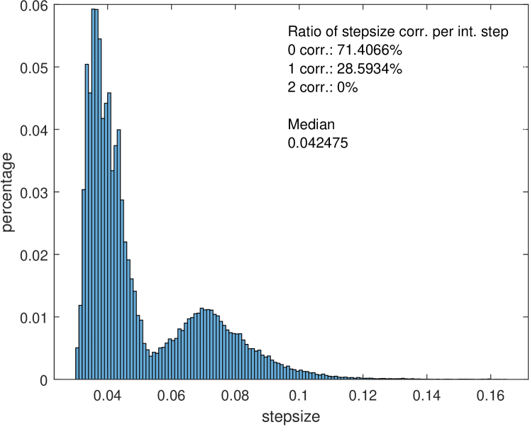
Refer to caption
(a) PDF of accepted stepsizes
Refer to caption
(b) LE1 (error)
Refer to caption
(c) LE2 (error)
Refer to caption
(d) LE3 (error)
Figure 1: The Lyapunov exponents of the system x˙=A(t)x˙𝑥𝐴𝑡𝑥\dot{x}=A(t)x from Subsection 5.1 are approximated using Benettin’s algorithm with different stepsizes. The first plot shows the PDF of the accepted stepsizes of the adaptive approach, while the other plots show the errors between computed Lyapunov exponents and their exact values. To save memory, the PDF was formed over every 101010th integration step.

Let

B(t)=(λ1f(t)00λ1000λ2)𝐵𝑡matrixsubscript𝜆1𝑓𝑡00subscript𝜆1000subscript𝜆2B(t)=\begin{pmatrix}\lambda_{1}&f(t)&0\\ 0&\lambda_{1}&0\\ 0&0&\lambda_{2}\end{pmatrix}

be a block-triangular matrix with λ1>λ2subscript𝜆1subscript𝜆2\lambda_{1}>\lambda_{2} and a bounded continuous function f𝑓f. One may check that the system y˙=B(t)y˙𝑦𝐵𝑡𝑦\dot{y}=B(t)y is regular and has stable Lyapunov exponents λ1subscript𝜆1\lambda_{1} and λ2subscript𝜆2\lambda_{2} due to Theorem 2.13. In particular, the system is fast-invertible at indices d1=2subscript𝑑12d_{1}=2 and d1+d2=3subscript𝑑1subscript𝑑23d_{1}+d_{2}=3. If we additionally assume that the integral of f𝑓f is bounded, then the system is fast-invertible at all indices. Hence, any system we obtain via Lyapunov transformations of y˙=B(t)y˙𝑦𝐵𝑡𝑦\dot{y}=B(t)y satisfies the assumptions for the dynamical system required in Theorem 4.2.

To get a specific example, we set λ1=1subscript𝜆11\lambda_{1}=1, λ2=0subscript𝜆20\lambda_{2}=0 and f(t)=sin(t)+1/(t2+1)𝑓𝑡𝑡1superscript𝑡21f(t)=\sin(t)+1/(t^{2}+1) and transform y˙=B(t)y˙𝑦𝐵𝑡𝑦\dot{y}=B(t)y to

x˙=A(t)x:=(LBL1+L˙L1)(t)x˙𝑥𝐴𝑡𝑥assign𝐿𝐵superscript𝐿1˙𝐿superscript𝐿1𝑡𝑥\dot{x}=A(t)x:=(LBL^{-1}+\dot{L}L^{-1})(t)x

using the composition L(t)𝐿𝑡L(t) of two Lyapunov transformations

(1sin(t)cos(t)01sin(t)001)(cos(2t)0sin(2t)010sin(2t)0cos(2t)).matrix1𝑡𝑡01𝑡001matrix2𝑡02𝑡0102𝑡02𝑡\begin{pmatrix}1&\sin(t)&\cos(t)\\ 0&1&\sin(t)\\ 0&0&1\end{pmatrix}\begin{pmatrix}\cos(\sqrt{2}t)&0&\sin(\sqrt{2}t)\\ 0&1&0\\ -\sin(\sqrt{2}t)&0&\cos(\sqrt{2}t)\end{pmatrix}.

The Lyapunov exponents are approximated using the different stepsizes mentioned in the beginning of Section 5. We start with the adaptive approach and take the median of the accepted stepsizes (Fig. 1(a)) as the constant stepsizes for the second approach. The approximated Lyapunov exponents of all approaches are compared to their exact values (Λ1=1subscriptΛ11\Lambda_{1}=1, Λ2=1subscriptΛ21\Lambda_{2}=1 and Λ3=0subscriptΛ30\Lambda_{3}=0) and plotted against the number of integration steps (Figs. 1(b), 1(c) and 1(d)).

For all three Lyapunov exponents, we see that errors persist with adaptive and constant stepsizes. Although we may reduce these persistent errors by decreasing the given tolerance or stepsize, we would have to rerun the algorithm for a longer time until the errors settle. On the other hand, the errors obtained with varying stepsizes show a steady decay as we would expect from our convergence theory.

5.2 Lorenz-63 model
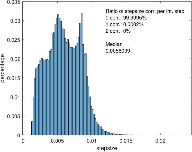
Refer to caption
(a) PDF of accepted stepsizes
Refer to caption
(b) LE1
Refer to caption
(c) LE2
Refer to caption
(d) LE3
Refer to caption
(e) LE2 (error)
Refer to caption
(f) LE sum (error)
Figure 2: The Lyapunov exponents of the Lorenz-63 model from Subsection 5.2 are approximated using Benettin’s algorithm with different stepsizes. The first plot shows the PDF of the accepted stepsizes of the adaptive approach, while the other plots show the computed Lyapunov exponents or their errors. To save memory, the PDF was formed over every 101010th integration step.

Our second example is the Lorenz-63 model [19] (a reduced model for thermal convection) given by the equations

x˙1=σ(x2x1)x˙2=x1(ρx3)x2x˙3=x1x2βx3}:=f(x)assigncasessubscript˙𝑥1𝜎subscript𝑥2subscript𝑥1subscript˙𝑥2subscript𝑥1𝜌subscript𝑥3subscript𝑥2subscript˙𝑥3subscript𝑥1subscript𝑥2𝛽subscript𝑥3𝑓𝑥\mathopen{}\mathclose{{}\left.\begin{array}[]{lll}\dot{x}_{1}&=&\sigma(x_{2}-x_{1})\\ \dot{x}_{2}&=&x_{1}(\rho-x_{3})-x_{2}\\ \dot{x}_{3}&=&x_{1}x_{2}-\beta x_{3}\end{array}}\right\}:=f(x)

with σ=10𝜎10\sigma=10, β=8/3𝛽83\beta=8/3 and ρ=28𝜌28\rho=28 as the classical parameters. The system is famous for its unpredictable behavior despite being deterministic. It exhibits a so-called strange attractor (the Lorenz attractor), which is a minimal attracting flow-invariant set that is neither a steady state nor a periodic orbit and which has a positive largest Lyapunov exponent121212For nonlinear systems, the Lyapunov exponents are obtained from the linearized flow along nonlinear trajectories. If the nonlinear system has an ergodic invariant measure, the Lyapunov exponents coincide for almost every trajectory. Hence, we may associate Lyapunov exponents with the attractor or measure instead of the trajectory.. So far, the existence of the attractor and the existence of a physical ergodic invariant measure (SRB measure) that admits a positive largest Lyapunov exponent is only known as a consequence of the computer-aided proof by Tucker [30].

To compute the Lyapunov exponents, we require a background trajectory lying on the attractor. This is problematic, since the Lorenz attractor has Lebesgue measure zero. In particular, the initial state of our background trajectory will almost surely lie outside of the attractor. While the trajectory may be close to the attractor after a transient, a rigorous analysis would require continuity properties of the Lyapunov exponents that extend to a neighborhood of the attractor. However, in general, the Lyapunov exponents vary only measurably with the base point. Moreover, integration errors can lead to an error of order O(1)𝑂1O(1) in the background trajectory as well as in the derived linear system. This may drastically change the computed Lyapunov exponents.

Despite the open challenges, we try to approximate the Lyapunov exponents and compare our methods for the known cases, that is, the second Lyapunov exponent and the sum of all Lyapunov exponents. The second Lyapunov exponent corresponds to the tangent vector of the background trajectory, which is a solution of the linearized equations that is neither exponentially growing nor decaying, and thus must be zero. The sum of all three Lyapunov exponents must be equal to the trace of the Jacobian, as it is constant. Indeed, it holds

Λ1+Λ2+Λ3=limt1tlog|det(X(t))|subscriptΛ1subscriptΛ2subscriptΛ3subscript𝑡1𝑡𝑋𝑡\displaystyle\Lambda_{1}+\Lambda_{2}+\Lambda_{3}=\lim_{t\to\infty}\frac{1}{t}\log\mathopen{}\mathclose{{}\left|\det\mathopen{}\mathclose{{}\left(X(t)}\right)}\right|
=limt1t0ttr(Df(x(s)))𝑑s=(σ+1+β)absentsubscript𝑡1𝑡superscriptsubscript0𝑡tr𝐷𝑓𝑥𝑠differential-d𝑠𝜎1𝛽\displaystyle\hskip 10.00002pt=\lim_{t\to\infty}\frac{1}{t}\int_{0}^{t}\textnormal{tr}(Df(x(s)))ds=-(\sigma+1+\beta)

for any solution x(t)𝑥𝑡x(t) along which the linearized system X(t)𝑋𝑡X(t) is regular. Exact values of the first and the third Lyapunov exponent are unknown.

The Lyapunov exponents are computed in a similar fashion to Subsection 5.1. This time, however, we require a background trajectory along which to propagate linear perturbations. In order to start close to the attractor, we first compute a transient starting from a randomly chosen state. After the transient, we couple the nonlinear system to its linearization. This way, we can compute the background trajectory and propagate linear perturbations simultaneously.

In this example, the adaptive approach requires almost no stepsize corrections (Fig. 2(a)) and is thus even closer to the other approaches in term of computational costs per step. As before, we observe that Lyapunov exponents computed with adaptive and constant stepsizes seem to converge to different values depending on the given tolerance or stepsize (Figs. 2(b), 2(c) and 2(d)). A meaningful comparison between the different approaches is only possible for the second and the sum of all Lyapunov exponents (Figs. 2(e) and 2(f)). We note that, similar to the linear example, adaptive and constant stepsizes can be better momentarily, while varying stepsizes eventually have the advantage in terms of accuracy.

5.3 Lorenz-96 model
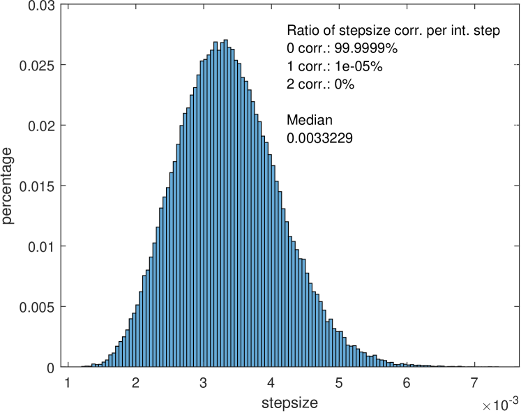
Refer to caption
(a) PDF of accepted stepsizes
Refer to caption
(b) LE spectrum
Refer to caption
(c) LE1
Refer to caption
(d) LE15
Refer to caption
(e) LE40
Refer to caption
(f) LE sum (error)
Figure 3: The Lyapunov exponents of the Lorenz-96 model from Subsection 5.3 are approximated using Benettin’s algorithm with different stepsizes. The first plot shows the PDF of the accepted stepsizes of the adaptive approach, the second plot shows the computed spectra after 107superscript10710^{7} integration steps (108superscript10810^{8} steps for the reference), and the other plots compare the computed Lyapunov exponents to the reference (final value after 108superscript10810^{8} steps in Figs. 3(c), 3(d) and 3(e)). To save memory, the PDF was formed over every 100100100th integration step.

Our third example is the Lorenz-96 model [20], which was created to test numerical weather prediction. The model simulates the effects of external forcing, damping and advection on a scalar physical quantity, which lives on a periodic lattice representing a circle of latitude. Different from the Lorenz-63 model, the Lorenz-96 model treats each variable on the lattice the same. By changing the number of variables, one may study the effects of increased spacial resolution on the predictability (or chaoticity) of the system. There already are studies of spatiotemporal chaos in the Lorenz-96 model in which spectra of Lyapunov exponents have been computed [14].

The Lorenz-96 model with d4𝑑4d\geq 4 variables is given by the equations

xi˙=(xi+1xi2)xi1xi+F˙subscript𝑥𝑖subscript𝑥𝑖1subscript𝑥𝑖2subscript𝑥𝑖1subscript𝑥𝑖𝐹\dot{x_{i}}=(x_{i+1}-x_{i-2})x_{i-1}-x_{i}+F

with periodic indices, i.e., xi+kd:=xiassignsubscript𝑥𝑖𝑘𝑑subscript𝑥𝑖x_{i+kd}:=x_{i} for k𝑘k\in\mathbb{Z}. We choose d=40𝑑40d=40 and a forcing parameter of F=10𝐹10F=10 to allow for chaotic dynamics. Under the same conditions, [14] computed the Lyapunov spectrum and noticed that the shape of the spectrum does not change while increasing the number of variables from 404040 to 505050. They used constant stepsizes of hn=1/64subscript𝑛164h_{n}=1/64 and integrated the trajectory for T=5×10⁵𝑇5superscript105T=5\times 10^{5} units of time or N=64T𝑁64𝑇N=64T timesteps. The first 2/3232/3 of the trajectory were used as a transient to approach the attractor before computing the Lyapunov exponents.

Here, we explore the effects of different stepsizes on the Lyapunov spectrum in terms of the approaches mentioned in the beginning of Section 5. Similar to the Lorenz-63 model, we know that at least one Lyapunov exponent must vanish and that the sum of all Lyapunov exponents must be equal to the trace of the Jacobian, which is d𝑑-d. However, it is not clear which index corresponds to the vanishing Lyapunov exponent. Instead, we compare the Lyapunov spectra of our different approaches to a reference spectrum computed with a high-resolution run. The latter is performed with ten times the number of integration steps than the other runs and with constant stepsizes that are ten times smaller than the constant stepsizes from the low-resolution run. While a higher resolution heuristically provides better estimates of the Lyapunov exponents, we still have to expect persistent errors.

Our computed Lyapunov spectra (Fig. 3(b)) take on similar shapes to the spectrum in [14, Fig. 5]. We see that the spectra computed with varying stepsizes are closer to the reference spectrum than the ones computes with adaptive or constant stepsizes. The differences between the spectra vary with the specific Lyapunov exponent. A more detailed picture showing the computed extremal Lyapunov exponents and the near-zero exponent can be seen in (Figs. 3(c), 3(d) and 3(e)). Concerning the sum of all Lyapunov exponents, we observe a similar behavior as in the other two examples (Fig. 3(f)).


6 Conclusions

There are multiple error sources in the computation of Lyapunov exponents. Errors can arise in both the nonlinear system and its linearization. Even in the absence of errors from the nonlinear system, integration errors can accumulate and result in persistent errors in the output of Benettin’s algorithm.

We observed these persistent errors in our three numerical examples. The first example was a linear system satisfying the requirements of our convergence theory, whereas the other two examples, the Lorenz-63 and the Lorenz-96 model, were nonlinear systems with chaotic attractors. In all three examples, we could see differences between the computed Lyapunov exponents. While adaptive and constant stepsizes resulted in persistent errors, varying stepsizes of the form hn=h/n2subscript𝑛2𝑛h_{n}=h/\sqrt[2]{n} and hn=h/n3subscript𝑛3𝑛h_{n}=h/\sqrt[3]{n} seemed to result in converge to the true Lyapunov exponents.

More general types of stepsizes were considered in our convergence analysis. We derived conditions for stepsizes under which Benettin’s algorithm converges in the presence of integration errors from the linear system. The first condition is that the sum of all stepsizes diverges, which is necessary for computing asymptotic quantities like the Lyapunov exponents, whereas the second condition ensures that the stepsizes decrease fast enough to prevent the accumulation of integration errors. Together with the assumptions of regularity and fast-invertibility, we proved convergence for the largest Lyapunov exponent before generalizing our results to multiple exponents via exterior powers.

Our numerical observations and theoretical results show that stepsize variations can improve the accuracy of Benettin’s algorithm. They counter the accumulation of integration errors and get rid of persistent errors that usually occur for adaptive or constant stepsizes. While we were able to partially verify our numerical observations analytically, we only considered linear systems. Errors from nonlinear systems require further analysis outside of this article. Finally, we can imagine additional improvements by combining our approach with weighted averaging or with adaptive stepsizes in terms of a varying tolerance parameter.


Acknowledgments

This paper is a contribution to the project M1 (Dynamical Systems Methods and Reduced Models in Geophysical Fluid Dynamics) of the Collaborative Research Centre TRR 181 “Energy Transfers in Atmosphere and Ocean” funded by the Deutsche Forschungsgemeinschaft (DFG, German Research Foundation) - Projektnummer 274762653.

Code availability

The code used to generate the data analyzed during this study was uploaded to [26].


References

  • [1] L. Adrianova “Introduction to linear systems of differential equations” v.146, Translations of mathematical monographs, 0065-9282 Providence, R.I.: American Mathematical Society, 1995
  • [2] Ludwig Arnold “Random Dynamical Systems”, Springer monographs in mathematics BerlinHeidelberg: Springer, 1998 DOI: 10.1007/978-3-662-12878-7
  • [3] Ludwig Arnold and Dinh Cong Nguyen “Linear cocycles with simple Lyapunov spectrum are dense in L-infty” In Ergodic Theory and Dynamical Systems 19.6, 1999, pp. 1389–1404 DOI: 10.1017/S014338579915199X
  • [4] E.. Barabanov and N.. Denisenko “Necessary and sufficient conditions for the stability of Lyapunov exponents of linear differential systems with exponentially decaying perturbations” In Differential Equations 43.2, 2007, pp. 168–179 DOI: 10.1134/S001226610702005X
  • [5] Giancarlo Benettin, Luigi Galgani, Antonio Giorgilli and Jean-Marie Strelcyn “Lyapunov Characteristic Exponents for smooth dynamical systems and for hamiltonian systems; a method for computing all of them. Part 1: Theory” In Meccanica 15.1, 1980, pp. 9–20 DOI: 10.1007/BF02128236
  • [6] Giancarlo Benettin, Luigi Galgani, Antonio Giorgilli and Jean-Marie Strelcyn “Lyapunov Characteristic Exponents for smooth dynamical systems and for hamiltonian systems; A method for computing all of them. Part 2: Numerical application” In Meccanica 15.1, 1980, pp. 21–30 DOI: 10.1007/BF02128237
  • [7] Luca Dieci, Michael S. Jolly and Erik S. van Vleck “Numerical Techniques for Approximating Lyapunov Exponents and Their Implementation” In Journal of Computational and Nonlinear Dynamics 6.1, 2011 DOI: 10.1115/1.4002088
  • [8] Luca Dieci and Erik S. van Vleck “LESLIS and LESLIL: Codes for approximating Lyapunov exponents of linear systems”, 2004 URL: https://dieci.math.gatech.edu/preps/les_reports/techreplin.pdf
  • [9] Luca Dieci and Erik S. van Vleck “On the error in computing Lyapunov exponents by QR Methods” In Numerische Mathematik 101.4, 2005, pp. 619–642 DOI: 10.1007/s00211-005-0644-z
  • [10] Luca Dieci and Erik S. van Vleck “Perturbation Theory for Approximation of Lyapunov Exponents by QR Methods” In Journal of Dynamics and Differential Equations 18.3, 2006, pp. 815–840 DOI: 10.1007/s10884-006-9024-3
  • [11] Luca Dieci and Erik S. van Vleck “On the Error in QR Integration” In SIAM Journal on Numerical Analysis 46.3, 2008, pp. 1166–1189
  • [12] F. Ginelli et al. “Characterizing Dynamics with Covariant Lyapunov Vectors” In Physical review letters 99.13, 2007, pp. 130601 DOI: 10.1103/PhysRevLett.99.130601
  • [13] Peter Grassberger and Itamar Procaccia “Measuring the strangeness of strange attractors” In Physica D: Nonlinear Phenomena 9.1-2, 1983, pp. 189–208 DOI: 10.1016/0167-2789(83)90298-1
  • [14] A. Karimi and M.. Paul “Extensive chaos in the Lorenz-96 model” In Chaos: An Interdisciplinary Journal of Nonlinear Science 20.4, 2010, pp. 043105 DOI: 10.1063/1.3496397
  • [15] Daniel Karrasch and George Haller “Do Finite-Size Lyapunov Exponents detect coherent structures?” In Chaos: An Interdisciplinary Journal of Nonlinear Science 23.4, 2013, pp. 043126 DOI: 10.1063/1.4837075
  • [16] Pavel V. Kuptsov and Ulrich Parlitz “Theory and Computation of Covariant Lyapunov Vectors” In Journal of Nonlinear Science 22.5, 2012, pp. 727–762 DOI: 10.1007/s00332-012-9126-5
  • [17] G.. Leonov and N.. Kuznetsov “Time-varying Linearization and the Perron effects” In International Journal of Bifurcation and Chaos 17.04, 2007, pp. 1079–1107 DOI: 10.1142/S0218127407017732
  • [18] M.. Liapounoff “Problème général de la stabilité du mouvement” In Annales de la Faculté des sciences de Toulouse: Mathématiques 9, 1907, pp. 203–474
  • [19] Edward N. Lorenz “Deterministic Nonperiodic Flow” In Journal of the Atmospheric Sciences 20, 1963, pp. 130–141 DOI: 10.1175/1520-0469(1963)020<0130:DNF>2.0.CO;2
  • [20] Edward N. Lorenz “Predictability – a problem partly solved” In Predictability of Weather and Climate Cambridge: Cambridge University Press, 2006, pp. 40–58 DOI: 10.1017/CBO9780511617652.004
  • [21] Edward J.. Mcdonald and Desmond Higham “Error analysis of QR algorithms for computing Lyapunov exponents” In Electronic Transactions on Numerical Analysis, 2001, pp. 234–251
  • [22] Dinh Cong Nguyen “A generic bounded linear cocycle has simple Lyapunov spectrum” In Ergodic Theory and Dynamical Systems 25.06, 2005, pp. 1775 DOI: 10.1017/S0143385705000337
  • [23] Dinh Cong Nguyen and Thai Son Doan “An open set of unbounded cocycles with simple Lyapunov spectrum and no exponential separation” In Stochastics and Dynamics 07.03, 2007, pp. 335–355 DOI: 10.1142/S0219493707002062
  • [24] Florian Noethen “A projector-based convergence proof of the Ginelli algorithm for covariant Lyapunov vectors” In Physica D: Nonlinear Phenomena 396, 2019, pp. 18–34 DOI: 10.1016/j.physd.2019.02.012
  • [25] Florian Noethen “Computing Covariant Lyapunov Vectors in Hilbert spaces” In Journal of Computational Dynamics 8.3, 2021, pp. 325–352 DOI: 10.3934/jcd.2021014
  • [26] Florian Noethen “Code for "Stepsize Variations for Lyapunov Exponents to Counter Persistent Errors" (v1.1)” Zenodo, 2023 DOI: 10.5281/zenodo.8013859
  • [27] Anthony Quas, Philippe Thieullen and Mohamed Zarrabi “Explicit bounds for separation between Oseledets subspaces” In Dynamical Systems 34.3, 2019, pp. 517–560 DOI: 10.1080/14689367.2019.1571562
  • [28] Shawn C. Shadden, Francois Lekien and Jerrold E. Marsden “Definition and properties of Lagrangian coherent structures from finite-time Lyapunov exponents in two-dimensional aperiodic flows” In Physica D: Nonlinear Phenomena 212.3-4, 2005, pp. 271–304 DOI: 10.1016/j.physd.2005.10.007
  • [29] I. Shimada and T. Nagashima “A Numerical Approach to Ergodic Problem of Dissipative Dynamical Systems” In Progress of Theoretical Physics 61.6, 1979, pp. 1605–1616 DOI: 10.1143/PTP.61.1605
  • [30] Warwick Tucker “A Rigorous ODE Solver and Smale’s 14th Problem” In Foundations of Computational Mathematics 2.1, 2002, pp. 53–117 DOI: 10.1007/s002080010018
  • [31] Christopher L. Wolfe and Roger M. Samelson “An efficient method for recovering Lyapunov vectors from singular vectors” In Tellus A: Dynamic Meteorology and Oceanography 59.3, 2007, pp. 355–366 DOI: 10.1111/j.1600-0870.2007.00234.x