Contrastive Object Detection Using Knowledge Graph Embeddings

Abstract

Object recognition for the most part has been approached as a one-hot problem that treats classes to be discrete and unrelated. Each image region has to be assigned to one member of a set of objects, including a background class, disregarding any similarities in the object types. In this work, we compare the error statistics of the class embeddings learned from a one-hot approach with semantically structured embeddings from natural language processing or knowledge graphs that are widely applied in open world object detection. Extensive experimental results on multiple knowledge-embeddings as well as distance metrics indicate that knowledge-based class representations result in more semantically grounded misclassifications while performing on par compared to one-hot methods on the challenging COCO and Cityscapes object detection benchmarks. We generalize our findings to multiple object detection architectures by proposing a knowledge-embedded design knowledge graph embedded (KGE)for keypoint-based and transformer-based object detection architectures.

1 Introduction

Object detection is the task of localizing and classifying objects in an image. Deep object detection originates from the two-stage approach [1, 2, 3] which first searches for anchor points in the image that potentially contain objects, followed by classifying and regressing the coordinates for each proposal region in isolation. The Faster R-CNN approach [1] achieves an average precision of 21.9% on the challenging COCO 2017 benchmark [4] for object detection in everyday situations. Its dependence on a heuristic suppression of multiple detections for the same object is a commonly addressed design flaw [5]. In an effort to make the network end-to-end trainable, recent architectures model the relationship between object proposals by formulating object detection as a keypoint detection [6, 7] or a direct-set estimation problem [8, 9, 10]. Such novel architectures along with stronger backbones [11, 12] and multiscale feature learning techniques [13, 14, 15] have doubled the average precision on the COCO detection benchmark to 54.0% [10].

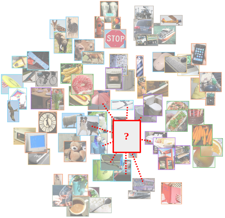
Figure 1: We incorporate class prototypes such as GloVE [16] from natural language processing, into the prediction head of common object detectors. The resulting feature space is structured by the context from non-visual knowledge sources such that similar concepts are in proximity, which we show yields more semantically-grounded predictions.

These astonishing benchmark performances have grown at the expense of a set-based classification formulation, i.e., the classes are regarded as discrete and unrelated. This assumption allows such methods to use a multinomial logistic loss [1, 17, 6] to boost the classification accuracy by maximizing the inter-class distances [18]. However, this forces the model to treat each class prototype out-of-context from what it has learned about the appearance of the other classes. As a result, the training is prone to inherit bias through class-imbalance [19, 20] or co-occurrence statistics [21] from the training data, and neglects synergies in the real world, where there exist semantic similarities between classes. This closed-set formulation further requires drastic changes of the class prototypes to be learned whenever the set of classes is extended [22, 23], resulting in catastrophic forgetting of previously learned classes when the training is performed incrementally [23, 24].

In zero-shot learning, that aims to detect classes that were excluded from the training set, the parametric class prototypes are replaced with a mapping from visual to a semantic embedding space, e.g. word embeddings generated from text corpora, which describe semantic context for a broad set of object classes. We extend this approach to keypoint-based and transformer-based object detectors and evaluate various knowledge embeddings as well as loss functions on the COCO 2017 [4] and Cityscapes [25] datasets. Additionally, we analyze the classification error distributions of our proposed KGE architectures with baseline methods of set-based classification and show that KGE predictions tend to be more semantically consistent with the groundtruth.

In summary, our main contributions in this work are:

• a knowledge embedding formulation for two-stage, keypoint-based and transformer-based multi-object detection architectures.

• a quantitative ablation study on the COCO 2017 over different distance metrics and knowledge types.

• an error overlap analysis between one-hot and embedding-based classifications.

2 Related Work

This work relates to the research areas of object detection architectures, especially their classification losses and the usage of commonsense knowledge in computer vision. In this section, we review the relevant works in these areas.

Object Detection: Two-stage methods [1, 2, 17] rely on a Region Proposal Network (RPN)to first filter image regions containing objects from a set of search anchors. In a second stage, a Region of Interest (RoI)head extracts visual features from which it regresses enclosing bounding boxes as well as predicts a class label from a multi-set of classes for each object proposal in isolation. Classification is then learned using a cross-entropy loss across the confidence scores for each class, including a background class, where the class labels are found by matching the groundtruth bounding boxes to object proposal boxes using only the intersection over union (IoU). This formulation is vulnerable to imbalanced class distributions in the training data, therefore a focal loss [19] down-weights well-classified examples in the cross-entropy computation to focus the training on hard examples.

Anchor-less detectors such as keypoint-based or center-based methods [26, 6, 7] embody an end-to-end approach that directly predicts objects as class-heatmaps. They use a logistic regression loss for training using multi-variate Gaussian distributions each centered at a groundtruth box. The classification stage has a global receptive field, which enables implicit modeling of context between detections. Transformer-based methods [8, 27, 10] currently lead the COCO 2017 [4] object detection benchmark. These methods detect objects using cross-attention between the learned object queries and visual embedding keys, as well as self-attention between object queries to capture their interrelations in the scene context. DETR [8] builds upon ResNet as a feature extractor and a transformer encoder to compute self-attention among all pixels of the feature map. However, the quadratic complexity w.r.t. the input resolution makes it infeasible for high-resolution feature maps, leading to poor performance on small objects. More efficient querying strategies, e.g., DeformableDETR [9], was proposed that also support multiscale feature maps.

Knowledge-based embeddings: In zero-shot classification [28, 29] and recognition [30, 31, 32, 33], word embeddings commonly replace learnable class prototypes to transfer from training classes to unseen classes using inherit semantic relationships extracted from text corpora. Commonly used word embeddings are GloVe vectors [29, 30] and word2vec embeddings [31, 34, 33, 35], however embeddings learnt from image-text pairs using the CLIP [36] achieve the best zero-shot performance so far [32]. Rahman et al. [31] argue that a single word embedding per class is insufficient to model the visual-semantic relationships and propose to learn class representations of weighted word embeddings of synonyms and related terms [31]. Nevertheless, pure text embeddings perform consistently best for training classes [30, 31, 32, 33, 35, 32] in object detection. The projection from visual to semantic space is done by a linear layer [30, 37, 35], a single  [31, 34, 33] or two-layer MLP [32], and learned with a max-margin losses [30, 31, 38, 37], softplus-margin focal loss [35], or cross-entropy loss [33, 32]. Zhang et. al. [39] suggests to rather a mapping from semantic to visual space to benefit to alleviate the hubness problem in semantic spaces, however, our analysis of COCO 2017 class vectors suggested that the hubness phenomena does not have a noticeable impact on the COCO 2017 class embedding space.

Another fundamental design choice in zero-shot object detection is the background class representation. The majority of works rely on an explicit class prototype that is either learned [33, 32], computed as the mean of all class vectors [31, 34, 37], or represented by multiple background word embeddings [30]. However, Li et al. [35] noted that an explicit representation can cause confusions with unknown classes and therefore represented background by a distance threshold w.r.t. each class prototype.

In this work, we analyze the usage of semantic relations between embeddings from the error distribution point of view and extend it to keypoint-based and transformer-based object detection architectures. We compare contrastive loss with margin-based loss functions and ablate multiple embedding sources to strengthen our analysis.

3 Technical Approach

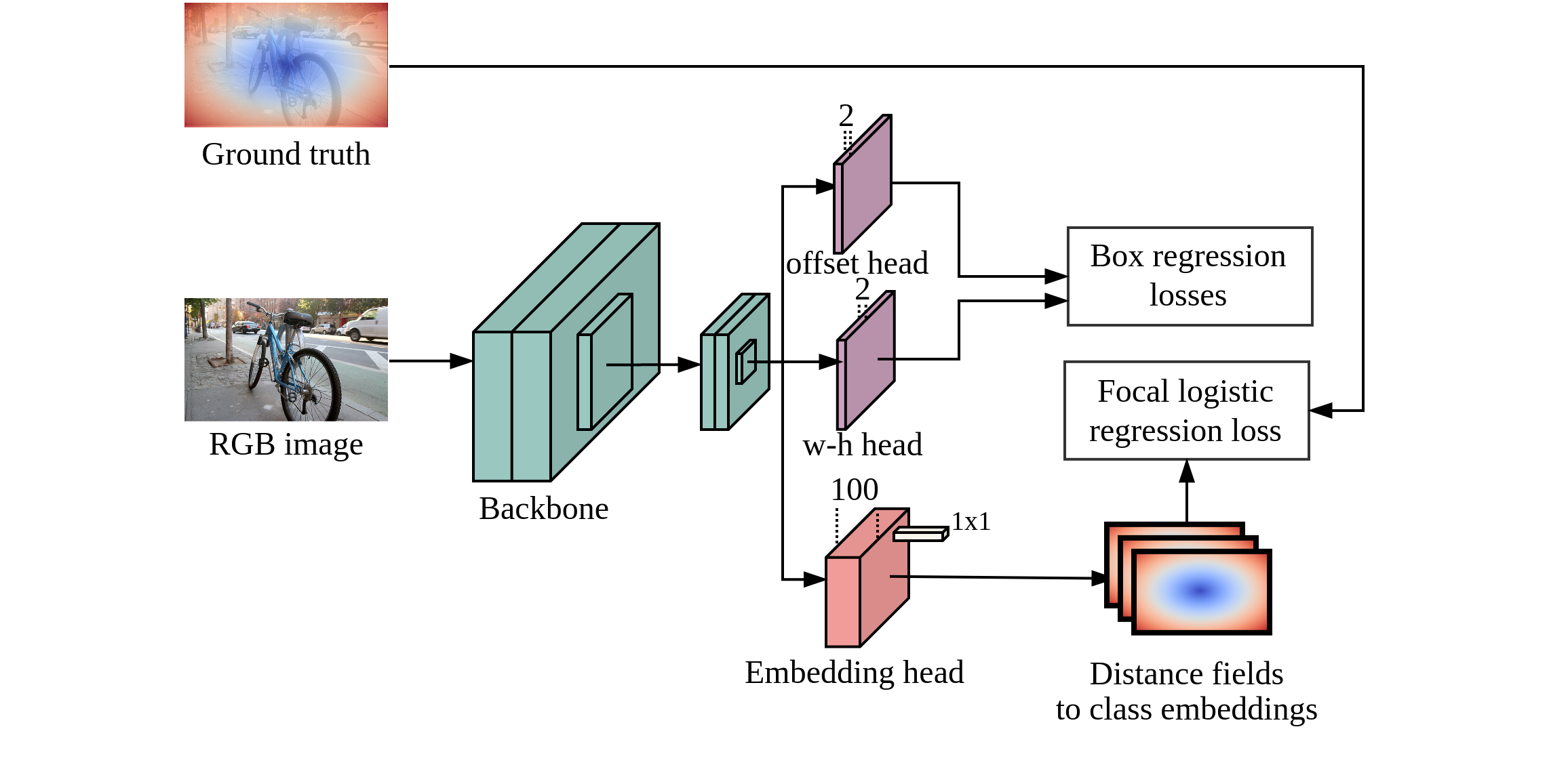
(a) Knowledge graph embedded (KGE) CenterNet.

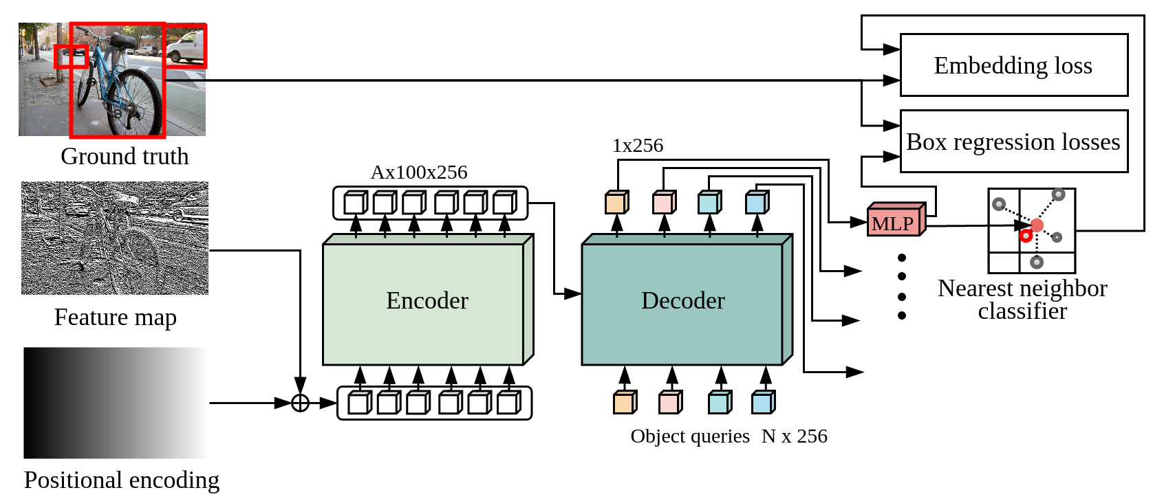
(b) Knowledge graph embedded (KGE) DETR object detection head.

Figure 2: Knowledge graph embedded architecture using nearest neighbor classifiers for CenterNet architecture (a) and a transformer-head (b). The CenterNet (a) encodes the image into a downscaled feature map from which it regresses a per-pixel class embedding vector, bounding box width and height, as well as centerpoint offset. Object localization is performed by computing distance fields to each class prototype. For all the distances lower than a background threshold, we perform a local minima search in an 8-connected neighborhood to locate object center points. DETR (b) employs a transformer encoder and decoder with object queries as keys to detect objects. The decoded values are fed into an MLP that outputs bounding box coordinates as well as an embedding vector that is used for nearest neighbor classification given semantic class prototypes.

Closed-set object detection architectures [1, 6, 8, 40] share a classification head $\mathbb{R}^{D}\mapsto\mathbb{R}^{C}$ design incorporating a linear output layer, that maps the feature vector into a vector of class scores of the form

$$p(y=c|\mathbf{x}_{i})=\textit{softmax}(\mathbf{W}^{T}\mathbf{x}_{i})_{c},$$ (1)

where $\mathbf{W}\in\mathbb{R}^{D\times C}$ is the parameter matrix of the linear layer, which effectively is composed of C learnable class prototypes. These parameters are learned with a one-hot loss formulation, incentivizing the resulting class prototypes to be pairwise orthogonal.

We replace learnable class prototypes with fixed object type embeddings that lend structure from external knowledge domains in the closed-set setting. Essentially, this entails replacing the direct estimation of classification scores in object detection with a regression that maps image regions into a shared space of visual features and semantic embedding vectors, where classification is done by a nearest neighbor search. In the remainder of this section, we present the possible class prototype choices in sec:object_representations, distance metrics in sec:distance_metrics, and describe the incorporation into two-stage detectors, keypoint-based method, and transformer-based architectures in sec:object_detector_integration.

3.1 Object-Type Embeddings

Instead of handcrafting the regression target vector or learning them from the training data, we incorporate object type embeddings from other knowledge modalities as follows:

• GloVe word embeddings [41] build on the descriptive nature of human language learned from a web-based text corpus. Human language reflects a variety of dependencies between objects -including causal, compositional, as well as spatial interrelations- which is expected to reflect in the embeddings.

• ConceptNet graph embeddings encode the conceptual knowledge between object categories entailed in the ConceptNet knowledge graphs [42]. The embeddings are computed by pointwise mutual information of the adjacency matrix and projected into a 100-D vector space by truncated SVG, as described by Speer et al. [42].

• COCO 2017 graph embeddings reflect the co-occurrence commonsense learned from the COCO 2017 training split. We build a heterogeneous graph from the spatial relations defined by Yatskar et al. [43]: {touches, above, besides, holds, on} and transform the resulting graph into node embeddings for each object prototype with an R-GCN [44].

3.2 Distance Metrics for Classification

We analyze nearest neighbor classification between visual embeddings of proposal boxes and object type representation vectors, either by the norm of the difference vector or angular distance. The $L_{k}$ norm of the difference vector between two embedding vectors is given by,

$$d_{k}(\overline{\mathbf{b}}_{i},\overline{\mathbf{t}}_{c})=\left(\sum_{d=1}^{D}\left(b_{i,d}-t_{c,d}\right)^{k}\right)^{1/k},$$ (2)

where $\mathbf{b}_{i}\in\mathbb{R}^{D}$ denotes the feature vector of the i-th proposal box and $\mathbf{t}_{c}\in\mathbb{R}^{D}$ the class prototype of the c-th object class. The maximum distance bound is given by the triangle inequality as $d_{k,max}\leq|\mathbf{t}_{c}|_{k}+|\mathbf{b}_{i}|_{k}$. In order to have a bound independent of $D$, we project all embeddings inside the unit sphere as

$$\overline{\mathbf{x}}=\frac{\mathbf{x}}{\max(1,|\mathbf{x}|_{2})}.$$ (3)

Since the relative contrast in higher dimensions is largest for low values of $k$ [45], we analyze the Manhattan distance where $k=1$. We further investigate nearest neighbors in terms of the cosine angle between two embedding vectors. The distance is computed using the negated cosine similarity as

$$d_{cos}(\mathbf{b}_{i},\mathbf{t}_{c})=1-\frac{\mathbf{b}_{i}^{T}\mathbf{t}_{c}}{|\mathbf{b}_{i}||\mathbf{t}_{c}|}.$$ (4)

We then interpret the negated distance as a similarity measure,

$$sim(\mathbf{b}_{i},\mathbf{t}_{c})=1-d(\mathbf{b}_{i},\mathbf{t}_{c})/2$$ (5)

and define the embedding losses as a contrastive loss towards the class embedding vectors given by

where $c_{i}$ is the label of the groundtruth box to which the proposal is matched. $\tau$ denotes a fixed scaling factor of the similarity vector, commonly referred to as temperature. We follow [46] and fix $\tau=0.07$. In case of a feature vector $\mathbf{b}_{i}$ that is assigned to the background label, we set $c=0$ and $sim(\mathbf{b}_{i},\mathbf{t}_{0})=0$, as there is no class representation vector that the feature embedding should have close distance too. Please refer to the supplementary material for a comparison to a margin-based loss function.

3.3 Generalization to Existing Object Detectors

In this section, we describe the embedding extension to three types of object detectors: two-stage detectors, keypoint-based methods, and transformer-based.

Two-stage detectors such as R-CNN based methods [1] pools latent features of each object proposals regions to fixed-size feature vector in the RoI head. These features are then processed in a box regressor and classifier to refine and classify the boxes for each proposal in isolation. The base method is trained with a standard Faster R-CNN loss, including a cross-entropy loss for bounding box classification. For the Faster R-CNN KGE method, we replace the cross-entropy classification loss for an embedding loss function, such that the linear layer learns a regression towards fixed class prototype vectors rather than mutually optimizing both. We therefore task the linear output layer to map from the RoI feature dimensionality to the embedding dimensionality $D$. We replaced the ReLU activation at the box head output layer with a hyperbolic tangent activation function (tanh) to avoid zero-capping the RoI feature vectors before the final linear layer.

Keypoint-based detectors formulates object detections as a keypoint estimation problem. CenterNet [6] uses these keypoints as the center of the bounding boxes. The output stage has a convolutional kernel with filter depth equal to the number of object classes, as well as additional output heads for center point regression, bounding box width, and height, etc. Max-pooling on class-likelihood maps yields a unique anchor for each object under the assumption that no two bounding boxes share a center point. The class-likelihood maps are trained with a focal logistic regression loss, where each groundtruth bounding box is represented by a bivariate normal distribution $Y_{xyc}$ with mean at the groundtruth center point and class-specific variances.

For the KGE formulation, we use the filter depth of the embedding output stage according to the number of embedding dimensions, thus learning an embedding for each pixel in the output map as shown in fig:system_architecture_centernet. Center point search then requires to compute a distance field of each pixel embedding to the class representation vectors. We formulate the embedding based focal loss as

where $sim(\mathbf{b}_{i},\mathbf{t}_{c})$ is a similarity function, $\alpha$ and $\beta$ are hyperparameters of the focal loss, and $Y_{xyc}$ is a heatmap where each groundtruth bounding box of class $c$ is represented by a bivariate normal distribution $Y_{xyc}$ at its center point coordinates $x$ and $y$, scaled such that $Y_{xyc}=1$.

Transformer-based methods [8, 9] adopt an encoder-decoder architecture to map a ResNet-encoded image to features of a set of object queries. The DETR encoder computes self-attention of pixels in the ResNet output feature map concatenated with a positional embedding. The decoder consists of cross-attention modules that extract features as values, whereby the query elements are of N object queries and the key elements are of the output feature maps from the encoder. These are followed by self-attention modules among object queries. Each feature vector is then independently decoded into prediction box coordinates and class labels with a 3-layer perceptron with ReLU activation [8], as depicted in fig:system_detr. The network is trained with a unique matching between proposal boxes and groundtruth boxes based on a classification cost with the negative log-likelihood of class labels, a generalized IoU loss as well as L1 regression loss on the bounding box coordinates.

				COCO 2017 val			COCO 2017 test-dev
Model	Backbone	Prediction Head	Params	AP	${\text{AP}_{w}}$	${\text{AP}_{cat,w}}$	AP	${\text{AP}_{50}}$	${AP_{75}}$	${\text{AP}_{S}}$	${\text{AP}_{M}}$	${\text{AP}_{L}}$
Faster R-CNN [1]	R50-FPN	Fast R-CNN	42 M	40.2	40.9	41.9	40.2	61.0	43.8	24.2	43.5	52.0
Faster R-CNN KGE	R50-FPN	ConceptNet-Cossim	42 M	39.3	41.6	43.5	39.4	59.7	43.4	24.1	41.3	49.8
CenterNet [6]	DLA	$3\times 3$ Conv + FFN	19 M	42.5	43.9	45.1	41.6	60.3	45.1	21.5	43.9	56.0
CenterNet KGE	DLA	GloVe-Cossim	19 M	44.2	45.5	47.3	44.6	63.6	49.2	29.4	47.0	53.5
DETR [8]	ResNet-50	3-layer FFN	41 M	42.0	40.3	41.2	42.0	62.4	44.2	20.5	45.8	61.1
DETR KGE	R50-FPN	ConceptNet-Cossim	41 M	43.2	42.9	43.6	43.3	65.3	45.8	22.9	45.9	59.8

Table 1: COCO 2017 test-dev and val results. The top section shows baseline results with learnable class prototypes and a one-hot loss, where test-dev results were taken from the referenced literature and val results were reproduced using their detectron2 implementations. The bottom section presents results using test time augmentations for the proposed regression heads that vary in the type of class prototypes representation. For each meta architecture, we chose the best performing prediction head on the validation set. The COCO 2017 val columns show the average precision of predicting the correct class or category, which we could only evaluate on the validation set.

We propose to replace the class label prediction with a feature embedding regression, and replace the classification cost function in the Hungarian matcher by the negative logarithm of the similarity measure, as described in sec:distance_metrics. We further replace the ReLU activation function of the second-last linear layer with a tanh activation function.

4 Experimental Evaluation

We evaluate the nearest neighbor classification heads for 2D object detection on the COCO 2017 and Cityscapes benchmarks. We use the mean average precision ($AP$) metric averaged over IoU $\in[0.5:0.05:0.95]$ (COCO’s standard metric) as the primary evaluation criteria. We also report the $AP_{w}$ where we weight each class by the number of groundtruth instances, the average precision across scales $AP_{S,M,L}$ and the categories $AP_{cat}$ for completeness. The latter is a novel metric first introduced in this paper, which is based on categorizing the 80 COCO 2017 thing classes into a total of 19 base categories by finding common parent nodes based on WUP similarity in the Google knowledge graph [47]. A true positive classification label hereby defines the correct category rather than class. Please refer to the supplementary material for an overview of object categories.

We chose the object detection task over image classification as it additionally requires predicting whether a proposed image region contains a foreground object. Ablation studies are performed on the validation set, and a architecture-level comparison is reported on the COCO 2017 test-dev and Cityscapes val datasets. For object detection algorithms, we compare Faster R-CNN [1] as representative for anchor-based methods, CenterNet [6] as keypoint-based object detector, and DETR [8] as transformer-based representative.

	Cityscapes val
Model	AP	${\text{AP}_{50}}$	${\text{AP}_{75}}$	${\text{AP}_{w}}$	${\text{AP}_{cat}}$
Faster R-CNN [1]	41.4	62.5	43.4	48.5	49.3
Faster R-CNN KGE	34.5	58.3	34.4	41.4	41.8
CenterNet KGE	42.2	63.4	44.4	51.7	52.2
DETR KGE	39.7	61.1	42.5	47.2	47.9

Table 2: Validation set results for the Cityscapes dataset. The top section shows baseline results in detectron2 with standard one-hot classification heads. The bottom section shows results for the proposed regression heads for the same configurations as in tab:results_val_coco.

4.1 Datasets

COCO is currently the most widely used object detection dataset and benchmark. The data depicts complex everyday scenes containing common objects in their natural context. Objects are labeled using per-instance segmentation to aid in precise object localization [4]. We use annotations for 80 ”thing” objects types in the 2017 train/val split, with a total of 886,284 labeled instances in 122,266 images. The scenes range from dining table close-ups to complex traffic scenes.

Cityscapes is a large-scale database that focuses on semantic understanding of urban street scenes. It provides object instance annotations for 8 classes of around 5000 fine annotated images captured in 50 cities during various months, daytime, and good weather conditions [25]. The scenes are extremely cluttered with many dynamic objects such as pedestrians and cyclists that are often grouped near one another or partially occluded.

4.2 Training Protocol

We use the PyTorch [48] framework for implementing all architectures, and we train our models on a system with an Intel Xenon@2.20GHz processor and NVIDIA TITAN RTX GPUs. For comparability, we use a ResNet-50 backbone with weights pre-trained as an image classifier on the ImageNet dataset for all experiments, and the same training configurations as reported in [1] for Faster R-CNN KGE, in [6] for CenterNet KGE, and as in [8] for DETR KGE configurations. We rescale the images to $640\times 480$ pixels and use random flipping as well as cropping for augmentation.

4.3 Quantitative Results

On the COCO 2017 test set in tab:results_val_coco, we compare our results against baselines from the original methods presented in sec:object_detector_integration. We expected the baselines methods to outperform our proposed knowledge graph embedded (KGE)prediction heads since they favor one-hot encoded class prototypes which are pairwise orthogonal and therefore maximize inter-class distances. Nevertheless, tab:results_val_coco shows that the knowledge-based class prototypes in the final classification layer can compete with their baseline configurations in terms of the $AP$ metrics. On the COCO 2017 test-dev benchmark, the CenterNet KGE outperforms its one-hot encoded counterparts by $+1.7\%$ , while the DETR KGE variant achieves an overall $AP$ of $43.2$. The Faster R-CNN KGE method does not outperform its baseline performance in average precision, however, the comparison of the $AP_{w}$ metric shows that this could be dependent on the test set’s class-distribution. The precision gain is largest for $AP_{75}$ over all the methods, where the KGE methods benefit from high accuracy bounding boxes.

We attribute this competitive performance of the KGE methods to the small temperature value of $\tau=0.07$, which was used as a hyperparameter for the contrastive loss function. As Kornblith et al. [18] noted, the temperature controls a tradeoff between the generalizability of penultimate-layer features and the accuracy on the target dataset. We performed a grid search over temperature parameters and found that accuracy drops considerably with larger temperature values, as shown in the supplementary material. Another interesting observation are the large $AP_{category,w}$ scores, where the KGE methods consistently outperform their baselines by greater than $1.5\%$. These results demonstrate that misclassifications are more often within the same category, in contrast to baseline methods that appear to confuse classes across categories.

The results on the Cityscapes val set are shown in tab:cityscapes_test_results. The CenterNet KGE variant achieves the best precision with $AP=42.2\%$. We should note, that for this dataset with only few classes that are highly related, the Faster R-CNN KGE methods performs worse than its baseline, mainly due to few accurately predicted bounding boxes as can be seen by the low $AP_{75}=34.4$.

4.4 Ablation Study

In this section, we compare three class prototype representations described in sec:object_representations to analyze which aspects of semantic context are most important for the object detection task and evaluate distance metrics used for classification.

Model	Class Prototypes			COCO 2017 val
	GloVe	ConceptNet	COCO 2017	AP	${AP_{50}}$	${AP_{75}}$
Faster R-CNN KGE	x			38.24	57.49	41.98
		x		40.39	61.98	41.58
			x	31.40	47.33	34.84
CenterNet KGE	x			41.37	59.23	45.24
		x		41.04	58.76	44.97
			x	41.07	58.94	45.09
DETR KGE	x			40.29	59.30	42.73
		x		41.40	61.20	43.92
			x	37.36	54.85	39.53

Table 3: Ablation study on COCO 2017 validation set results over knowledge embeddings in 100 dimensions using a cossim distance metric and a contrastive loss ((6)). The class prototypes are described in sec:object_representations

Analysis of Object Type Representations: tab:results_ablation_embeddings shows the average precision for the object detection architectures presented in sec:object_detector_integration when using various class prototype representations on the COCO 2017 val set. The ConceptNet embedding gives the best $AP$ over the Faster R-CNN KGE and DETR KGE configurations, however the results for using a GloVe embedding performs best for the CenterNet architecture. The COCO embeddings consistently perform the worst for all KGE configurations. This is exceptional, since the COCO embeddings summarize the co-occurrence statistics without domain shift, while the ConceptNet and GloVe embeddings introduce external knowledge from textual and conceptual sources. These results indicate that the semantic contexts’ role is dominated by categorical knowledge about the object classes. Context from co-occurrence statistics appears to generate insufficient class separation for object types that are frequently overlapping, etc., resulting in a comparably large gap for Faster R-CNN when comparing COCO 2017 to the remaining embedding types.

Model	Distance Metric		COCO 2017 val
	Cosine similarity	Manhattan distance	AP	${AP_{50}}$	${AP_{75}}$
Faster R-CNN KGE	x		40.39	61.98	41.58
		x	35.99	56.88	38.87
CenterNet KGE	x		41.37	59.23	45.24
		x	16.42	22.97	18.57
DETR KGE	x		41.40	61.20	43.92
		x	40.37	60.16	42.70

Table 4: Ablation study on COCO 2017 validation set results over distance metrics for configurations using ConceptNet embeddings in 100 dimensions as class prototypes.

Analysis of Distance Metric: In tab:results_ablation_distance, we further compare validation set results for Manhattan and cosine distances in the nearest neighbor classification. The latter achieves consistently higher average precision values over all the architectures. The gap is largest for the CenterNet architecture, where the cosine similarity variant achieves $+24.7$ higher $AP$ and lowest for DETR with $+1.02AP$. This might reflect the sensitivity to outliers for each method and the separation of the embedding space. In high dimensions, the euclidean distance between two points is inherently large, since the vector becomes increasingly sparser. According to Aggarwal et al.[45], this results in decreasing contrast by the $L_{k}$-norm distance between embedding vectors with increasing dimensionality, which hurts classification performance. The cosine similarity on the other hand reports the same similarity between each point on a line from the origin to a target point, in principle reserving the scaling dimension to account for different appearances of an object class. Further, the effect of outlier values in a single dimension only enters the distance metric at most linearly.

4.5 Misclassification Analysis

We analyze the confusion matrix of each detector on the COCO 2017 validation split. The confusion matrix $\mathbf{E}\in\mathrm{R}^{C\times C}$ contains a row for each object class, and each entry represents the counts of predicted labels for this class groundtruth instances. For each groundtruth box, we select the predicted bounding box with the highest confidence score of all predicted boxes with an IoU $\geq 0.8$, i.e., each groundtruth box is assigned to at most one prediction.

For comparing error distributions of different object detectors, we compute the Jensen-Shannon distance of corresponding rows in the confusion matrices as

$$JS(\mathbf{p},\mathbf{q})=\sqrt{\frac{D(\mathbf{p}\parallel\mathbf{m})+D(\mathbf{q}\parallel\mathbf{m})}{2}},$$ (8)

where $\mathbf{p}$, $\mathbf{q}$ are false positive distributions, $\mathbf{m}$ is the point-wise mean of two vectors as $m_{i}=\frac{p_{i}+q_{i}}{2}$, and $D$ is the Kullback-Leibler divergence.

A low JS distance implies that the classification stages of the two detectors under comparison produce similar error distributions and vice versa. fig:js_distances_coco shows the JS distances for each object detection algorithm between the baseline method and all embedding-based prediction heads. We note that the error distributions vary noticeably from the baselines methods, however all the embedding-based prediction heads appear to differ by similar magnitudes. This behavior indicates that there is a conceptual difference in the prediction characteristic of the learned (baseline) and knowledge-based class prototypes. The effect is largest for the CenterNet architecture, presumably since the embedding-based formulation affects the classification as well as localization head. To further investigate the origin of this dissimilar behavior, we quantify the inter-category confusions of different object detector architectures in fig:supercategory_confusion.

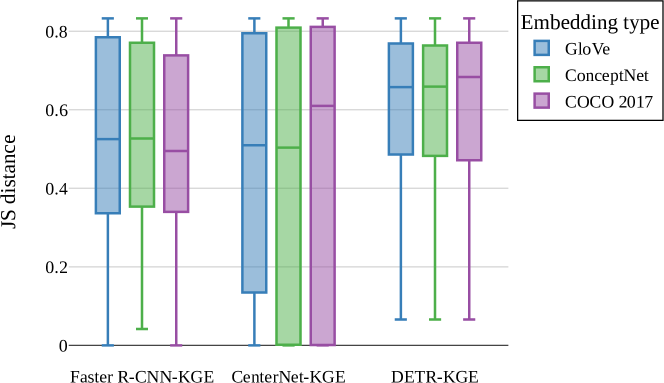
Figure 3: Jensen-Shannon distance between classification error distributions of detector type in baseline configuration compared to its variants using the knowledge-embedded class-prototypes described in sec:object_detector_integration.

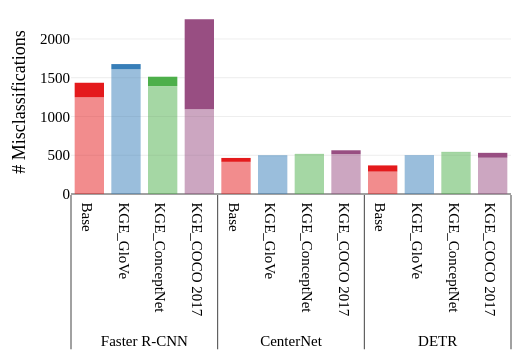
Figure 4: Misclassifications on the COCO 2017 validation split for each detector configuration. Light colors represent if the misclassified label has a common node with the groundtruth class in the Google knowledge graph [47] (intra-category confusion), solid colors indicate that there is no common parent node (inter-category confusion).

Inter-Category Confusion: fig:supercategory_confusion shows that all knowledge-embedded class prototypes, except for the COCO 2017 class prototypes, produce lower inter-category confusions compared to their one-hot encoded configurations. This signifies that feature embeddings derived from spatial relations between objects provide insufficient inter-class distances when used as class prototypes. This impairment is especially noticeable for the Faster R-CNN architecture, where class confusion of overlapping objects can also occur during the loss computation. The ConceptNet embeddings result in the lowest counts of inter-category confusion, since its structure is derived from a conceptual knowledge graph similar to the one used for categorization, and its inter-category confusion counts are consistently lower than the base configuration with learnable class prototypes.

4.6 Qualitative Results

	(a) image id 0a4c0fa7a6fa9280	(b) image id cb32cbcc6fb40d2a	(c) image id 0a4aaf88891062bf	(d) image id 4fb0e4b6908e0e56
Faster R-CNN
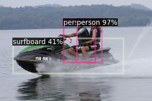
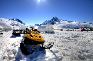
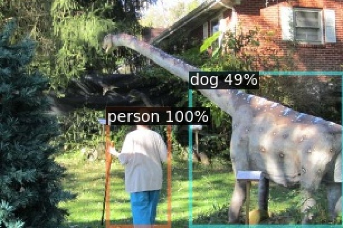
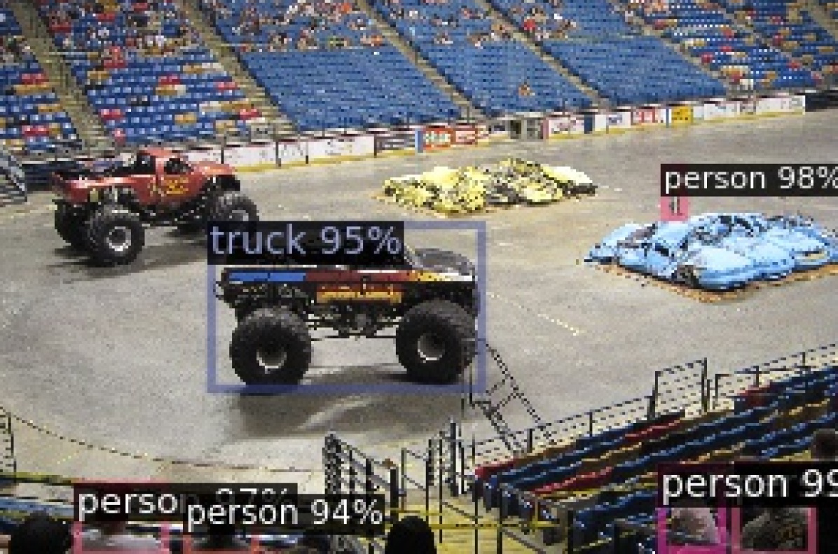
Faster R-CNN KGE
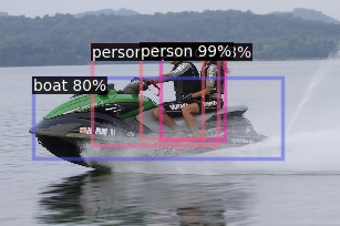
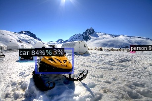
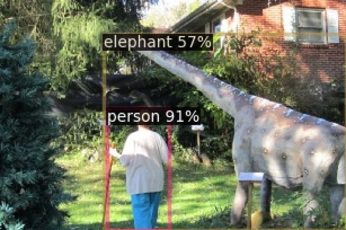
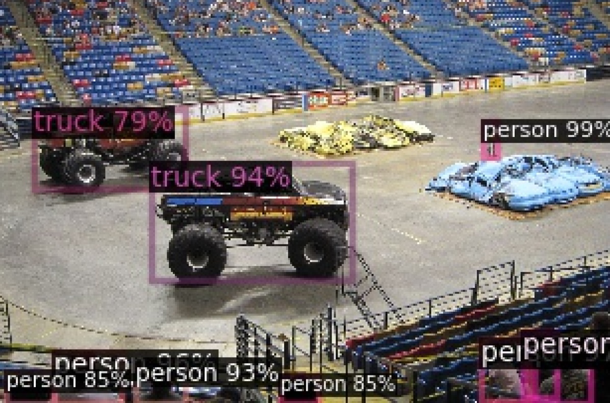
CenterNet
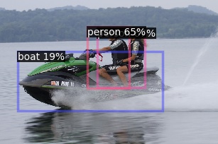
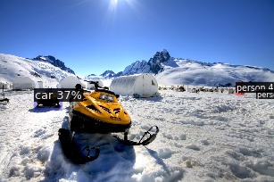
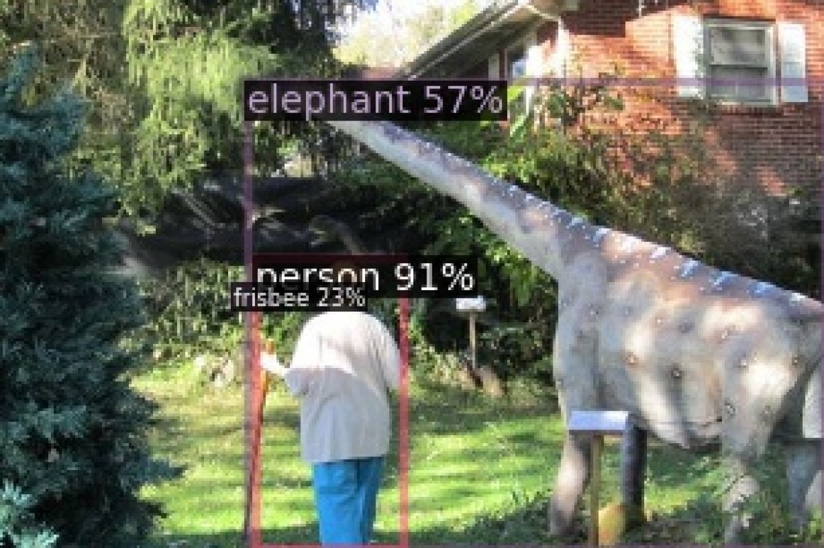
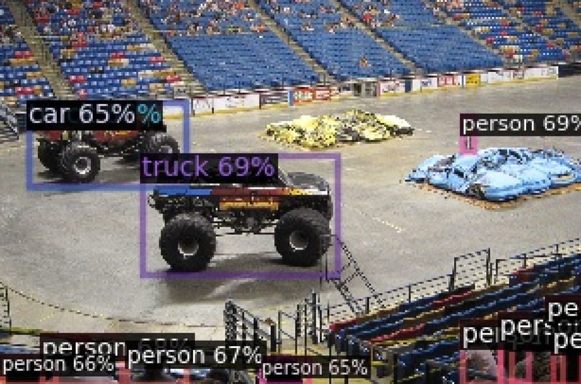
CenterNet KGE
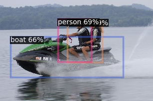
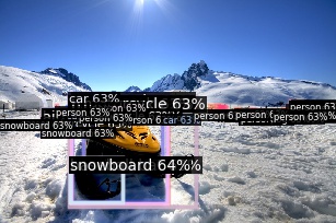
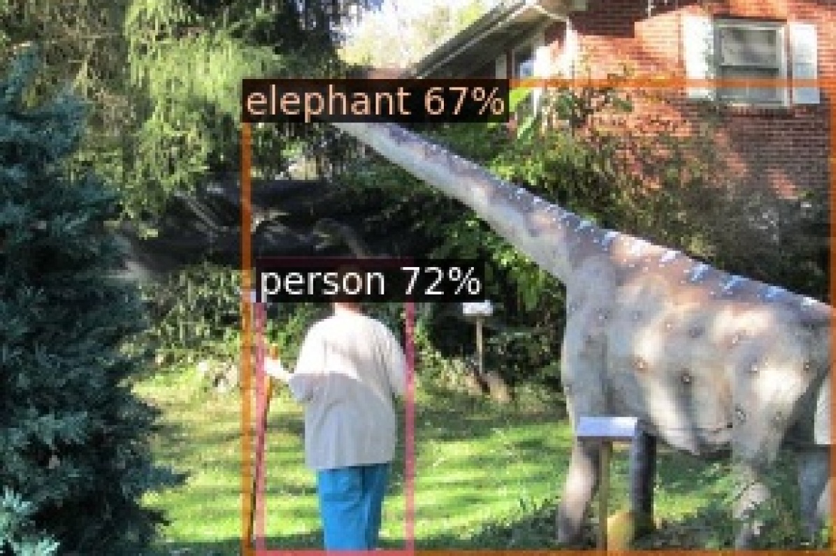
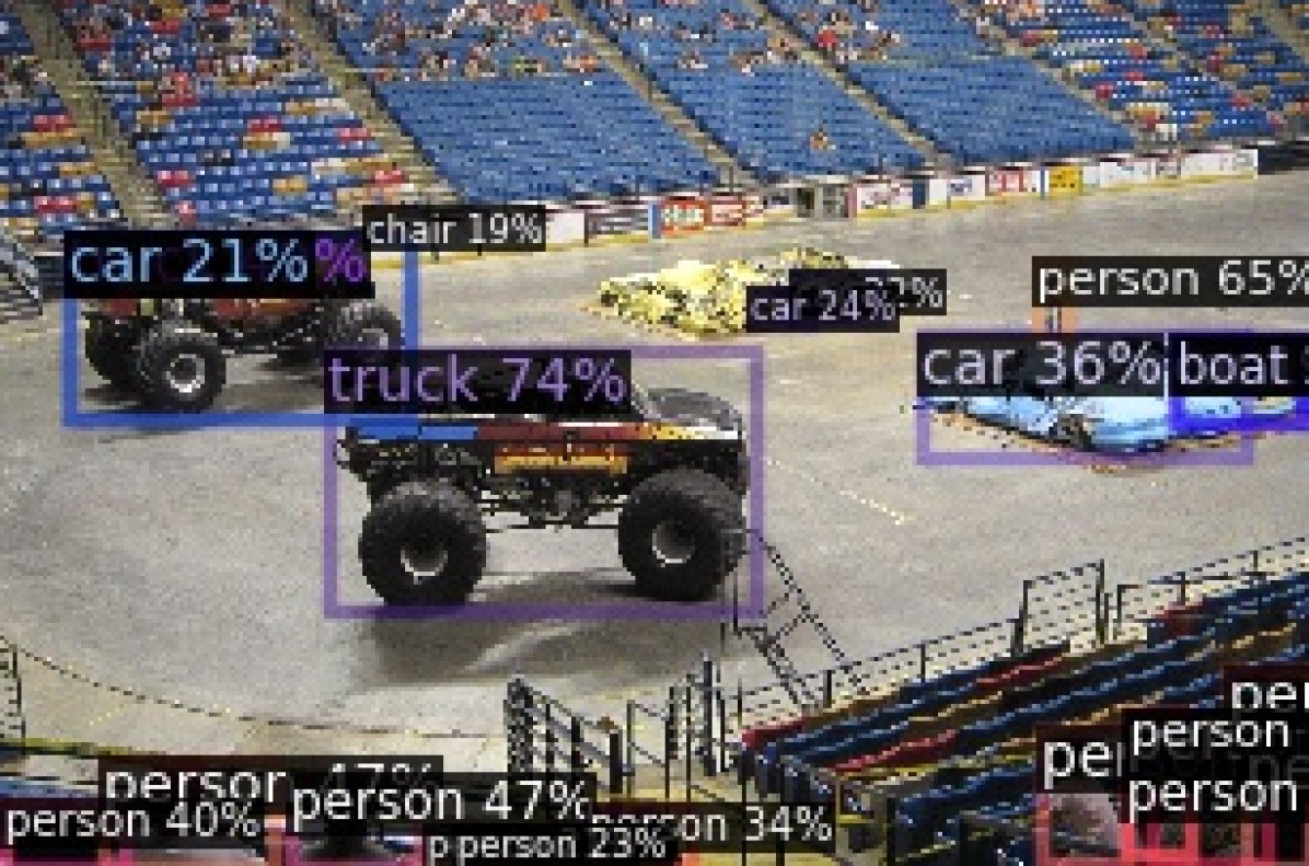
DETR
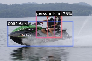
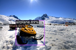
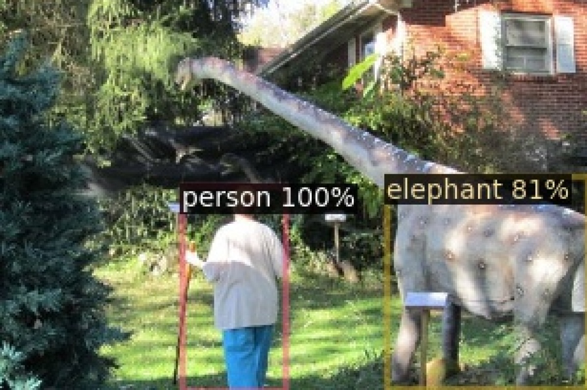
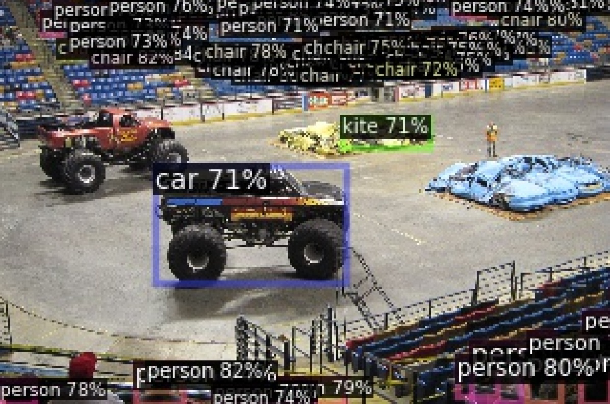
DETR KGE

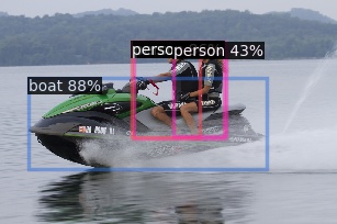
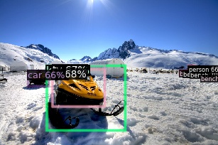
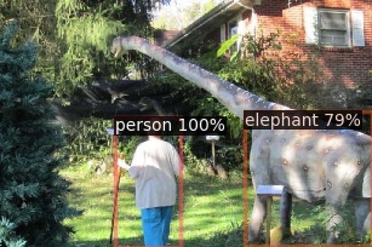
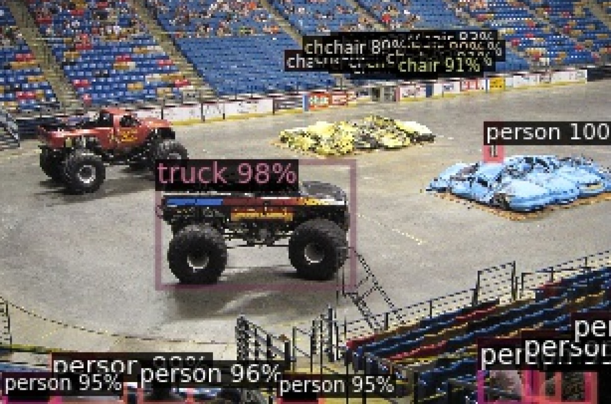
Figure 5: Qualitative results on images from the OpenImages  [49] validation set using the configurations in tab:results_val_coco. Please note that confidence scores for KGE methods describe the normalized similarity value between class prototype and visual embeddings.

We further qualitatively evaluate images from the OpenImages dataset [49] to demonstrate behavior on unseen objects and data distributions for methods trained on COCO 2017 dataset and classes. The results are shown in fig:qual-analysis. All the methods demonstrate high object localization accuracy, where foreground region regression appears correlated with the choice of detection architecture. The KGE-based detection heads have consistently lower confidence on the detections, however, they skew the object classification to more semantically related classes, e.g. the unknown snow mobile in fig:qual-analysis(b) is assigned to related classes such as car, snowboard, or motorcycle by the KGE methods, rather than airplane, boat, or truck by the baseline methods. The KGE methods also exhibit fewer false positives, such as the surfboard for Faster R-CNN in fig:qual-analysis(a) or kite in fig:qual-analysis(d) for DETR, which are not captured by the average precision metric on the object detection benchmarks.

5 Conclusions

In this work, we demonstrate the transfer of feature embeddings from natural language processing or knowledge graphs as class prototypes into two-stage, keypoint-based, and transformer-based object detection architectures trained using a contrastive loss. We performed extensive ablation studies that analyze the choice of class prototypes and distance metrics on the COCO 2017 and Cityscapes datasets. We showed that our resulting method can compete with their standard configurations on challenging object detection benchmarks, with error distributions that are more consistent with the object categories in the groundtruth. Especially, class prototypes derived from the ConceptNet knowledge graph [42] using a cosine distance metric demonstrate low inter-categorical confusions. Future work will investigate whether these knowledge embeddings in the classification head also benefit the class-incremental learning task in object detection.

Contrastive Object Detection Using Knowledge Graph Embeddings

Supplementary Material

Christopher Lang^1,2          Alexander Braun¹          Abhinav Valada^2
1Robert Bosch GmbH          ²University of Freiburg
christopher.lang@de.bosch.com            valada@cs.uni-freiburg.de

In this supplementary material, we provide additional insights and experimental results on knowledge embedding-based object detection.

1 Object Type Representation

First, we inspect the knowledge embeddings that we incorporated as class prototypes into the object detection architectures. fig:pairwise_cossine summarizes the pairwise distances among a subset of the COCO 2017 [4] classes for each knowledge embedding. Please note that we exploit the symmetry of the distance metrics, and show cosine (upper triangle) and Manhattan distance (lower triangle) alongside in the same plot. The metrics share the main diagonal, as they are both zero for identical input vectors. The distances are bounded by $d(\mathbf{x}_{1},\mathbf{x}_{2})\in[0,2]$, since the embedding vectors are normalized for the calculation of the cosine distance, respectively projected into the unit sphere for the calculation of the Manhattan distance.

In fig:pairwise_cossine (a), we extracted the class prototypes from the penultimate layer of a Faster R-CNN [1] model trained on the COCO 2017 dataset using a cross-entropy loss and learnable class prototypes. The method tends to maximize the pairwise distances among the class prototypes without semantic structure, except for weak clusters among groups of vehicle, animal, furniture, or food classes.

fig:pairwise_cossine (b) — (d) show the fixed class prototypes that were used during the experiments. Compared to the learned prototypes in (a), the distances are less uniform, reflecting the inherent semantic structure of the embeddings. The COCO embeddings (fig:pairwise_cossine (b)) have noticeably low inter-class distances and depict clusters of commonly co-occurring objects such as vehicles, furniture, and pets, as well as foods. In the GloVe embedding [16] (fig:pairwise_cossine (c)), we observe the most irregular distances end especially two outlier classes, such as bear or dining table, that have large distances to all other class embeddings. The ConceptNet embeddings [42] seem most similar to the learned embeddings with large inter-class distances, however, the inter-class distances show categorical differences, for example between furniture for sitting and lying, and vehicles for driving, swimming, or flying. The categorization of classes is shown in fig:class_hierarchy. The categorization originates from traversing the Google knowledge graph [47] starting from the COCO 2017 classes as leaf nodes and stopping at the first common parent node of each pair of classes. [4]

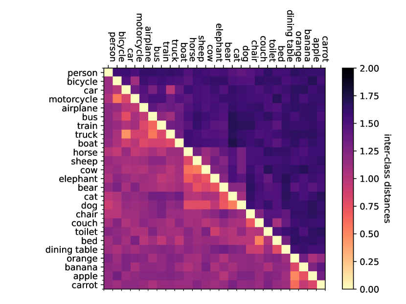
(a) Faster R-CNN trained embeddings, $D=1024$.

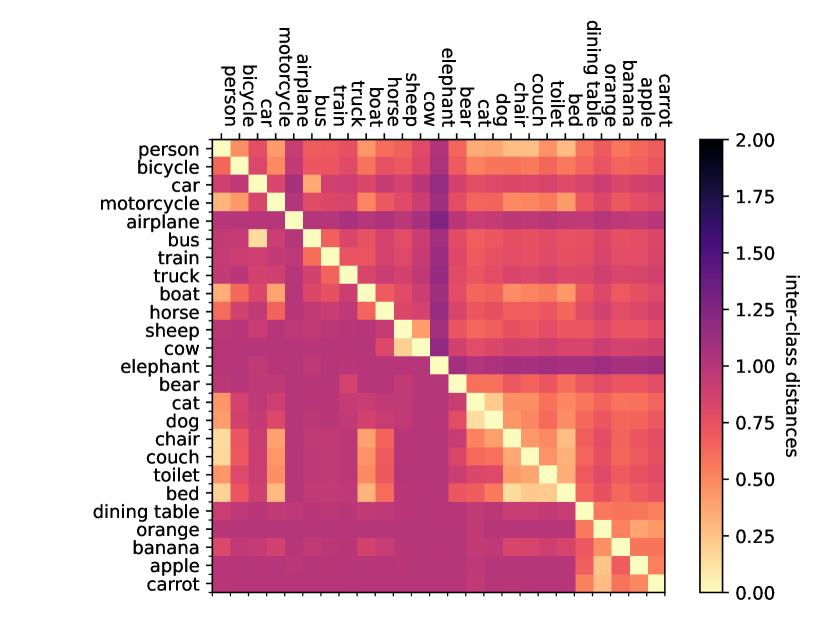
(b) COCO [4] spatial graph embeddings, $D=100$.

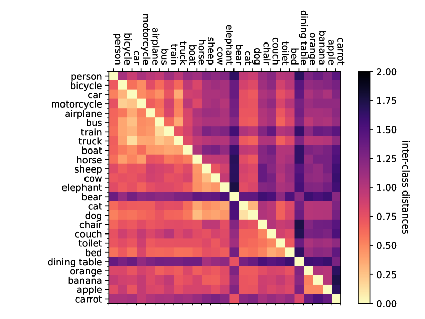
(c) GloVe word embeddings [16], $D=100$.

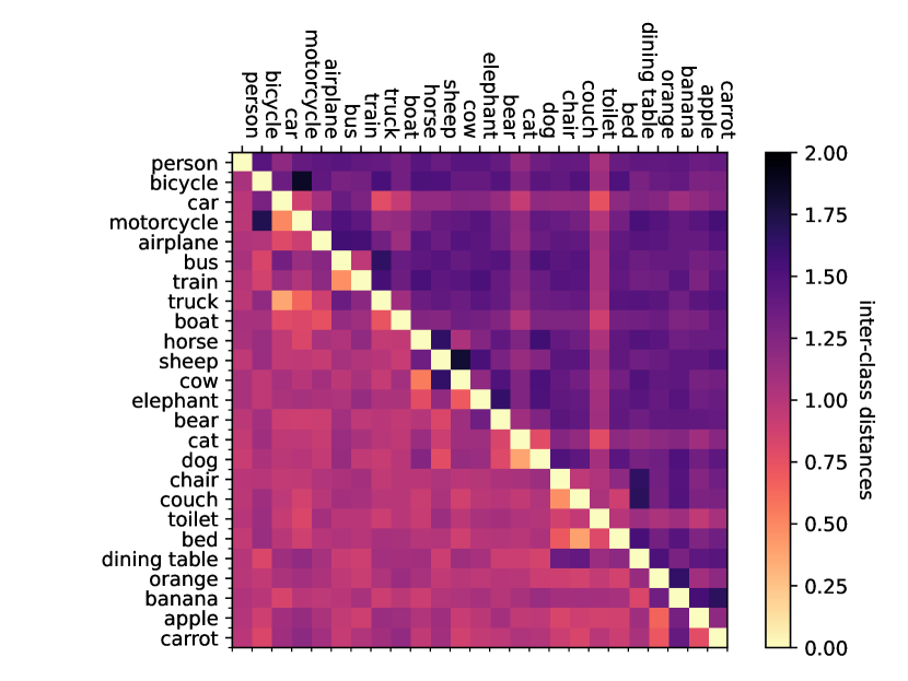
(d) ConceptNet graph embeddings [42], $D=100$.

Figure 1: Pairwise distances matrix of class prototypes. Since the distance metrics are symmetric, we show cosine distances in the upper triangle and bounded Manhattan distances in the lower triangle.

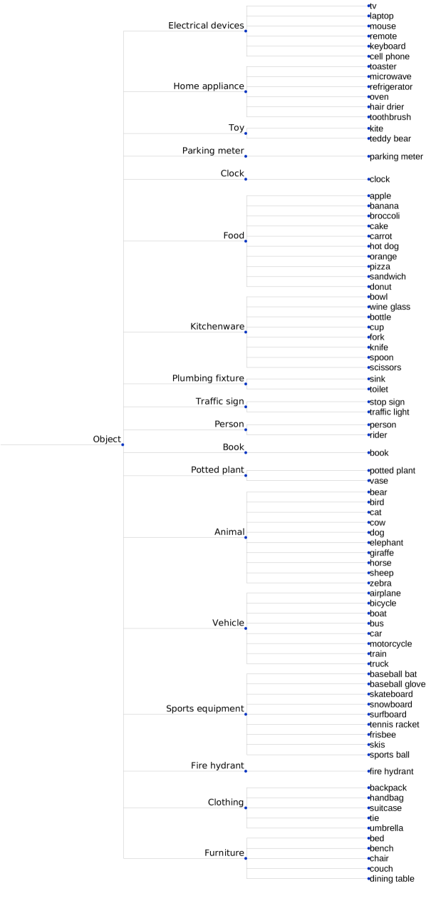
Figure 2: COCO class hierarchies extracted from the Google Knowledge Graph [47]. Categories are found from finding common parent nodes among all COCO 2017 thing classes in the graph. The node identifiers are taken from the OpenImages [49] class descriptions for matching object type labels.

		COCO 2017 val
Distance metric	Background representation	AP	${AP_{w}}$	${AP_{cat,w}}$
Cossim	Explicit	39.4	41.4	42.7
Cossim	Implicit	39.3	41.6	43.5
Manhattan	Explicit	36.0	38.1	38.9
Manhattan	Implicit	37.0	39.3	40.5

Table 1: Ablation study of Faster R-CNN KGE on the COCO 2017 validation set results over background representations using ConceptNet embeddings in 100 dimensions as class prototypes. Explicit background representations handle background regions as an additional class prototype vector for which nearest neighbor classification is performed, implicit background representations assign a background label based on a class confidence threshold.

2 Extended Ablation Study

In this section, we motivate the design choices we that make for the KGE object detection heads. We therefore ran experiments on the Faster R-CNN [1] base model using our proposed KGE extension as described in the main paper.

2.1 Explicit vs Implicit background representation

The application of nearest neighbor classification brings the design choice of how to represent the background class. tab:results_ablation_background shows our results when comparing an explicit background representation by an additional background class prototype, or an implicit representation by a distance threshold to all foreground class representations. We found that an explicit representation results in marginally higher $AP$, however, this appears to be a misconception due to the non-weighted mean, while an implicit representation achieves higher $AP_{w}$ and $AP_{category,w}$ for the cosine distance metric. For Manhattan distances, the implicit representation surpasses the explicit representation on all metrics.

In our benchmark experiments, we choose an implicit background representation, motivated by the larger $AP_{category,w}$, which we interpret as an indicator of more semantically-grounded errors.

2.2 Contrastive vs. Margin Loss

We experimented with both contrastive and margin embedding losses. One representative of the latter is the Hinge embedding loss that, given a proposal embedding $\mathbf{b}_{i}$, minimizes the distance to the true class prototype while enforcing a fixed margin $\Delta$ to all other class prototypes as follows:

where $y_{i,c}$ is an indicator variable, that is $1$ if a proposal box $i$ is assigned a groundtruth bounding box of class $c$ by a matching algorithm (e.g., IoU-based or Hungarian matching), and $-1$ for all other classes. In our experiments, we set the distance margin to $\Delta=\max\{0.1,d(\mathbf{t}_{c},\mathbf{t}_{f})\}$, i.e., the distance between the true class embedding $\{\mathbf{t}_{c}|y_{i,c}=1\}$ and all other class embeddings $\{\mathbf{t}_{f}|y_{i,f}=-1\}$ during training. Another hyperparameter is the negative sampling rate $r$ which denotes the number of randomly selected class prototypes other than the groundtruth class embedding evaluated for one proposal box embedding, for which we compute the margin loss term. For these experiments, we sample $r=5$ negative pairings uniformly from the set of COCO 2017 classes excluding the true class. As we can see from tab:results_ablation_embedding, the choice of embedding loss goes along with the distance metric that we use. A margin loss with a Manhattan distance metric achieves the highest $AP$ and $AP_{w}$. However, the contrastive loss performs better with a cosine distance metric and achieves the highest overall $AP_{category,w}$ with $43.5\%$. We choose the contrastive loss as it spares us two hyperparameters, the fixed margin $\Delta$ and negative sampling rate $r$, with a negligible decline in average precision.

		COCO 2017 val
Distance metric	Embedding loss	AP	${AP_{w}}$	${AP_{cat,w}}$
Cossim	Margin	36.4	38.7	38.9
Cossim	Contrastive	39.3	41.6	43.5
Manhattan	Margin	39.7	41.8	43.0
Manhattan	Contrastive	37.0	39.3	40.5

Table 2: Ablation study of Faster R-CNN KGE on COCO 2017 validation set results over embedding loss configurations using ConceptNet embeddings in 100 dimensions as class prototypes.

	COCO 2017 val
Contrastive loss $\tau$	AP	${AP_{w}}$	${AP_{cat,w}}$
1.0	32.5	36.1	40.3
0.1	33.0	36.1	40.1
0.07	39.3	41.6	43.5

Table 3: Ablation study of Faster R-CNN KGE on COCO 2017 validation set results over temperature values for the contrastive loss using ConceptNet embeddings in 100 dimensions as class prototypes.

		COCO 2017 val
Distance metric	z-scores standardization	AP	${AP_{w}}$	${AP_{cat,w}}$
Cossim		39.3	41.6	43.5
Cossim	x	36.6	40.8	41.6
Manhattan		37.0	39.3	40.5
Manhattan	x	34.7	40.3	42.6

Table 4: Ablation study of Faster R-CNN KGE on COCO 2017 validation set results over standardization strategies using ConceptNet embeddings in 100 dimensions as class prototypes.

2.3 High vs. Low Temperature Contrastive Losses

In the next step, we evaluated the inverse magnitude scaling parameter in the contrastive loss function, the so-called temperature $\tau$. Kornblith et al. [18] noted that this parameter is a trade-off between generalizability and precision on the training data. tab:results_ablation_temperature shows the temperature parameter’s effect on the validation set performance. High values for $\tau$ result in lower $AP$s since the distances are bounded by the interval $d\in[0,2]$, which results in flat scores after the approximate softmax scaling of the contrastive loss computation and thus low gradients. As we aim to achieve competitive performance as the baselines using cross-entropy losses, we follow [46] and fix $\tau=0.07$.

	(a) image id 0a1dae152634618c	(b) image id fd81aed21b5d54b8	(c) image id 3a0b72a274530636	(d) image id 040ad403d9c14ee2
Faster R-CNN
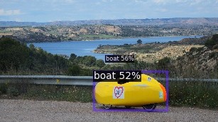
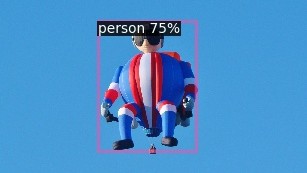
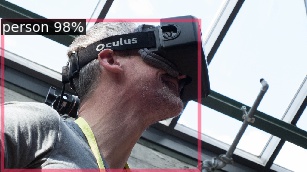
Faster R-CNN KGE
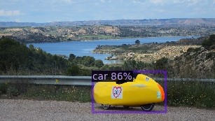
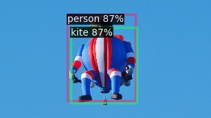
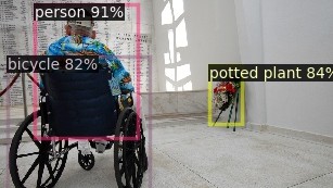
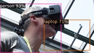
CenterNet
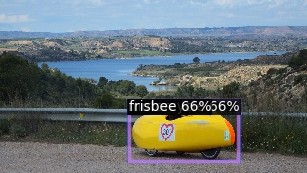
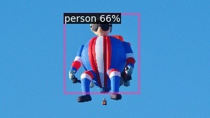
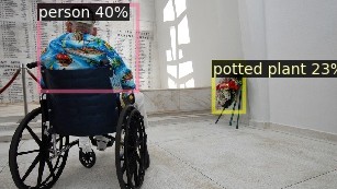
CenterNet KGE
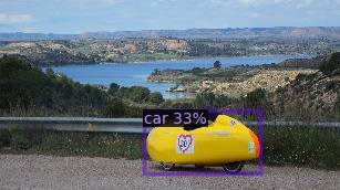
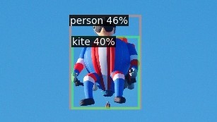
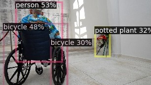
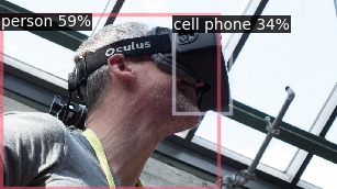
DETR
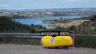
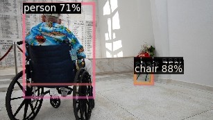
DETR KGE

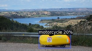
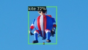
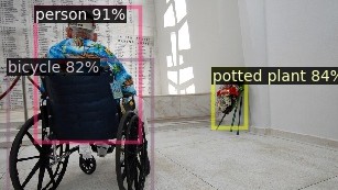
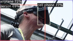
Figure 3: Qualitative results on images from the OpenImages [49] validation set using KGE configurations with cosine distance and ConceptNet [42] class prototypes. Please note that confidence scores for KGE methods describe the normalized similarity value between class prototype and visual embeddings.

2.4 Hubness Reduction vs. No Hubness Reduction

Fei et al. [50] recently raised awareness for the hubness problem in image classification. The hubness problem is a phenomenon that concerns nearest neighbor classification in high dimensional spaces. It relates to the distance concentration effect and results in few class prototypes being particularly often among the nearest neighbors of embeddings, while others are almost never. They report that local feature scaling by z-score standardization can reduce hubness in image classification. In this work we aim to validate whether z-score standardization can improve the classification accuracy as indirectly measured by the $AP$.

The results presented in tab:results_ablation_standardization shows that a hubness reduction measure such as z-score standardization does not improve $AP$ for neither cosine nor Manhattan distance. On the contrary, it hinders convergence of the training, such that the resulting validation set performance is worse when using z-score normalization. Therefore, we conclude that the fixed knowledge embeddings already bring sufficient training data and internal structure to alleviate hubs in the feature space.

3 Extended Qualitative Results

In this section, we discuss the out-of-distribution predictions on the OpenImages [49] dataset shown in fig:qual-analysis-supp, for models trained on COCO 2017 data and classes. In general, we observe that the object detectors mostly detect and localize all foreground objects in the frame, even if they are from unknown classes. The KGE modification appears to predominantly impact the classification scores and results in more semantically-grounded class predictions. For instance, the velomobile in fig:qual-analysis-supp (a) is classified as car or motorcycle by the KGE models, rather than boat, Frisbee, or airplane as observed in the predictions from the standard methods. The same holds for the pilot-shaped hot air balloon in fig:qual-analysis-supp (b), which is consistently identified as a kite using the knowledge-embedded class prototypes.

The KGE methods also predict reasonable high confidences to more abstract objects such as the wheelchair or VR goggles in fig:qual-analysis-supp (c) or fig:qual-analysis-supp (d), while the standard models classify such objects as background. The KGE methods produce overall lower confidence scores compared to their non-KGE counterparts, however, this is due to the variable inter-class distances in the knowledge embeddings.

References

- [1] S. Ren, K. He, R. Girshick, and J. Sun, “Faster r-cnn: Towards real-time object detection with region proposal networks,” in Proc. of the Conf. on Neural Information Processing Systems, 2015, pp. 91–99.
- [2] Z. Cai and N. Vasconcelos, “Cascade r-cnn: Delving into high quality object detection,” in Proc. of the IEEE Conf. on Computer Vision and Pattern Recognition, 2018, pp. 6154–6162.
- [3] F. R. Valverde, J. V. Hurtado, and A. Valada, “There is more than meets the eye: Self-supervised multi-object detection and tracking with sound by distilling multimodal knowledge,” in Proc. of the IEEE Conf. on Computer Vision and Pattern Recognition, 2021, pp. 11 612–11 621.
- [4] T.-Y. Lin, M. Maire, S. Belongie, J. Hays, P. Perona, D. Ramanan, P. Dollár, and C. L. Zitnick, “Microsoft coco: Common objects in context,” in Europ. Conf. on Computer Vision, 2014, pp. 740–755.
- [5] S. Liu, D. Huang, and Y. Wang, “Adaptive nms: Refining pedestrian detection in a crowd,” in Proc. of the IEEE Conf. on Computer Vision and Pattern Recognition, 2019, pp. 6459–6468.
- [6] X. Zhou, D. Wang, and P. Krähenbühl, “Objects as points,” arXiv preprint arXiv:1904.07850, 2019.
- [7] H. Law and J. Deng, “Cornernet: Detecting objects as paired keypoints,” in Europ. Conf. on Computer Vision, 2018, pp. 734–750.
- [8] N. Carion, F. Massa, G. Synnaeve, N. Usunier, A. Kirillov, and S. Zagoruyko, “End-to-end object detection with transformers,” in Europ. Conf. on Computer Vision, 2020, pp. 213–229.
- [9] X. Zhu, W. Su, L. Lu, B. Li, X. Wang, and J. Dai, “Deformable DETR: Deformable Transformers for End-to-End Object Detection,” arXiv preprint arXiv:2010.04159, 2020.
- [10] X. Dai, Y. Chen, B. Xiao, D. Chen, M. Liu, L. Yuan, and L. Zhang, “Dynamic head: Unifying object detection heads with attentions,” in Proc. of the IEEE Conf. on Computer Vision and Pattern Recognition, 2021, pp. 7373–7382.
- [11] K. He, X. Zhang, S. Ren, and J. Sun, “Deep residual learning for image recognition,” in Proc. of the IEEE Conf. on Computer Vision and Pattern Recognition, 2016, pp. 770–778.
- [12] K. Sirohi, R. Mohan, D. Büscher, W. Burgard, and A. Valada, “Efficientlps: Efficient lidar panoptic segmentation,” arXiv preprint arXiv:2102.08009, 2021.
- [13] T.-Y. Lin, P. Dollár, R. Girshick, K. He, B. Hariharan, and S. Belongie, “Feature pyramid networks for object detection,” in Proc. of the IEEE Conf. on Computer Vision and Pattern Recognition, 2017, pp. 2117–2125.
- [14] S. Qiao, L.-C. Chen, and A. Yuille, “Detectors: Detecting objects with recursive feature pyramid and switchable atrous convolution,” in Proc. of the IEEE Conf. on Computer Vision and Pattern Recognition, 2021, pp. 10 213–10 224.
- [15] N. Gosala and A. Valada, “Bird’s-eye-view panoptic segmentation using monocular frontal view images,” arXiv preprint arXiv:2108.03227, 2021.
- [16] J. Pennington, R. Socher, and C. D. Manning, “Glove: Global vectors for word representation,” in Proc. of the Conf. on Empirical Methods in Natural Language Processing, 2014, pp. 1532–1543.
- [17] P. Sun, R. Zhang, Y. Jiang, T. Kong, C. Xu, W. Zhan, M. Tomizuka, L. Li, Z. Yuan, C. Wang et al., “Sparse r-cnn: End-to-end object detection with learnable proposals,” in Proc. of the IEEE Conf. on Computer Vision and Pattern Recognition, 2021, pp. 14 454–14 463.
- [18] S. Kornblith, H. Lee, T. Chen, and M. Norouzi, “Why do better loss functions lead to less transferable features?” arXiv preprint arXiv:2010.16402, 2021.
- [19] T.-Y. Lin, P. Goyal, R. Girshick, K. He, and P. Dollár, “Focal loss for dense object detection,” Proc. of the IEEE Conf. on Computer Vision and Pattern Recognition, pp. 2980–2988, 2017.
- [20] K. He, G. Gkioxari, P. Dollar, and R. Girshick, “Mask R-CNN,” Int. Conf. on Computer Vision, pp. 2980–2988, 2017.
- [21] K. K. Singh, D. Mahajan, K. Grauman, Y. J. Lee, M. Feiszli, and D. Ghadiyaram, “Don’t judge an object by its context: Learning to overcome contextual bias,” in Proc. of the IEEE Conf. on Computer Vision and Pattern Recognition, 2020, pp. 11 070–11 078.
- [22] K. Shmelkov, C. Schmid, and K. Alahari, “Incremental learning of object detectors without catastrophic forgetting,” in Int. Conf. on Computer Vision, 2017, pp. 3400–3409.
- [23] J.-M. Perez-Rua, X. Zhu, T. M. Hospedales, and T. Xiang, “Incremental few-shot object detection,” in Proc. of the IEEE Conf. on Computer Vision and Pattern Recognition, 2020, pp. 13 846–13 855.
- [24] J. Zürn, W. Burgard, and A. Valada, “Self-supervised visual terrain classification from unsupervised acoustic feature learning,” IEEE Transactions on Robotics, vol. 37, no. 2, pp. 466–481, 2020.
- [25] M. Cordts, M. Omran, S. Ramos, T. Rehfeld, M. Enzweiler, R. Benenson, U. Franke, S. Roth, and B. Schiele, “The cityscapes dataset for semantic urban scene understanding,” in Proc. of the IEEE Conf. on Computer Vision and Pattern Recognition, 2016, pp. 3213–3223.
- [26] Z. Tian, C. Shen, H. Chen, and T. He, “Fcos: Fully convolutional one-stage object detection,” Proc. of the IEEE Conf. on Computer Vision and Pattern Recognition, pp. 9627–9636, 2019.
- [27] J. Yang, C. Li, P. Zhang, X. Dai, B. Xiao, L. Yuan, and J. Gao, “Focal self-attention for local-global interactions in vision transformers,” arXiv preprint arXiv:2107.00641, 2021.
- [28] Z. Akata, S. Reed, D. Walter, H. Lee, and B. Schiele, “Evaluation of output embeddings for fine-grained image classification,” in Proc. of the IEEE Conf. on Computer Vision and Pattern Recognition, 2015, pp. 2927–2936.
- [29] X. Wang, Y. Ye, and A. Gupta, “Zero-shot recognition via semantic embeddings and knowledge graphs,” in Proc. of the IEEE Conf. on Computer Vision and Pattern Recognition, 2018, pp. 6857–6866.
- [30] A. Bansal, K. Sikka, G. Sharma, R. Chellappa, and A. Divakaran, “Zero-shot object detection,” in Europ. Conf. on Computer Vision, 2018, pp. 384–400.
- [31] S. Rahman, S. Khan, and N. Barnes, “Improved visual-semantic alignment for zero-shot object detection,” in Proc. of the AAAI Conference on Artificial Intelligence, vol. 34, no. 07, 2020, pp. 11 932–11 939.
- [32] X. Gu, T.-Y. Lin, W. Kuo, and Y. Cui, “Open-vocabulary Object Detection via Vision and Language Knowledge Distillation,” arXiv preprint arXiv:2104.13921, 2021.
- [33] Y. Zheng, R. Huang, C. Han, X. Huang, and L. Cui, “Background learnable cascade for zero-shot object detection,” in Proc. of the Asian Conf. on Computer Vision, 2020.
- [34] S. Rahman, S. H. Khan, and F. Porikli, “Zero-shot object detection: Joint recognition and localization of novel concepts,” Int. Journal of Computer Vision, vol. 128, no. 12, pp. 2979–2999, 2020.
- [35] Q. Li, Y. Zhang, S. Sun, X. Zhao, K. Li, and M. Tan, “Rethinking semantic-visual alignment in zero-shot object detection via a softplus margin focal loss,” Neurocomputing, vol. 449, pp. 117–135, 2021.
- [36] A. Radford, J. W. Kim, C. Hallacy, A. Ramesh, G. Goh, S. Agarwal, G. Sastry, A. Askell, P. Mishkin, J. Clark et al., “Learning transferable visual models from natural language supervision,” arXiv preprint arXiv:2103.00020, 2021.
- [37] D. Gupta, A. Anantharaman, N. Mamgain, V. N. Balasubramanian, C. Jawahar et al., “A multi-space approach to zero-shot object detection,” in Proc. of the IEEE/CVF Winter Conf. on Applications of Computer Vision, 2020, pp. 1209–1217.
- [38] A. Frome, G. S. Corrado, J. Shlens, S. Bengio, J. Dean, M. A. Ranzato, and T. Mikolov, “Devise: A deep visual-semantic embedding model,” Proc. of the Conf. on Neural Information Processing Systems, vol. 26, 2013.
- [39] L. Zhang, T. Xiang, and S. Gong, “Learning a deep embedding model for zero-shot learning,” in Proc. of the IEEE Conf. on Computer Vision and Pattern Recognition, 2017, pp. 2021–2030.
- [40] J. V. Hurtado, R. Mohan, W. Burgard, and A. Valada, “Mopt: Multi-object panoptic tracking,” arXiv preprint arXiv:2004.08189, 2020.
- [41] J. Pennington, R. Socher, and C. D. Manning, “GloVe: Global Vectors for Word Representation,” in Empirical Methods in Natural Language Processing, 2014, pp. 1532—-1543.
- [42] R. Speer, J. Chin, and C. Havasi, “Conceptnet 5.5: An open multilingual graph of general knowledge,” in Proc. of the AAAI Conference on Artificial Intelligence, 2017.
- [43] M. Yatskar, V. Ordonez, and A. Farhadi, “Stating the obvious: Extracting visual common sense knowledge,” Conference of the North American Chapter of the Association for Computational Linguistics: Human Language Technologies,, pp. 193–198, 2016.
- [44] S. Woo, D. Kim, K. Daejeon, D. E. Cho, I. E. So Kweon, I. S. Kweon, and D. E. Cho, “LinkNet: Relational embedding for scene graph,” Proc. of the Conf. on Neural Information Processing Systems, pp. 560–570, 2018.
- [45] C. C. Aggarwal, A. Hinneburg, and D. A. Keim, “On the surprising behavior of distance metrics in high dimensional space,” Int. Conf. on Database Theory, pp. 420–434, 2001.
- [46] F. Wang and H. Liu, “Understanding the Behaviour of Contrastive Loss,” arXiv preprint arXiv:2012.09740, pp. 2495–2504, 2020.
- [47] “Google Knowledge Graph.” [Online]. Available: https://developers.google.com/knowledge-graph
- [48] A. Paszke, S. Gross, F. Massa, A. Lerer, J. Bradbury, G. Chanan, T. Killeen, Z. Lin, N. Gimelshein, L. Antiga, A. Desmaison, A. Kopf, E. Yang, Z. DeVito, M. Raison, A. Tejani, S. Chilamkurthy, B. Steiner, L. Fang, J. Bai, and S. Chintala, “Pytorch: An imperative style, high-performance deep learning library,” in Proc. of the Conf. on Neural Information Processing Systems, H. Wallach, H. Larochelle, A. Beygelzimer, F. d'Alché-Buc, E. Fox, and R. Garnett, Eds., 2019, pp. 8024–8035.
- [49] A. Kuznetsova, H. Rom, N. Alldrin, J. Uijlings, I. Krasin, J. Pont-Tuset, S. Kamali, S. Popov, M. Malloci, A. Kolesnikov, T. Duerig, and V. Ferrari, “The open images dataset v4: Unified image classification, object detection, and visual relationship detection at scale,” Int. Journal of Computer Vision, 2020.
- [50] N. Fei, Y. Gao, Z. Lu, and T. Xiang, “Z-score normalization, hubness, and few-shot learning,” in Proc. of the IEEE Conf. on Computer Vision and Pattern Recognition, 2021, pp. 142–151.