Random normal matrices in the almost-circular regime

Abstract.

We study random normal matrix models whose eigenvalues tend to be distributed within a narrow “band” around the unit circle of width proportional to $\frac{1}{n}$, where $n$ is the size of matrices. For general radially symmetric potentials with various boundary conditions, we derive the scaling limits of the correlation functions, some of which appear in the previous literature notably in the context of almost-Hermitian random matrices. We also obtain that fluctuations of the maximal and minimal modulus of the ensembles follow the Gumbel or exponential law depending on the boundary conditions.

1. Introduction

In non-Hermitian random matrix theory, one often encounters annular domains in the limiting spectral distribution of certain models. A typical example of such a model is the induced Ginibre ensemble [22], an extension of the Ginibre ensemble to include zero eigenvalues. This model is described with two parameters $a_{n}$ and $b_{n}$ $(a_{n}>b_{n})$, which possibly depend on the size $n$ of the matrix. Here, the former parameter $a_{n}$ is related to the scaling factor and the latter one $b_{n}$ is related to the zero modes of the model. (See (1.2) and (1.3) below for a precise description.) Then the eigenvalues $\{\zeta_{j}\}_{1}^{n}$ of the induced Ginibre ensemble tend to be uniformly distributed on the annulus

(1.1) $$S_{n}^{I}:=\Big{\{}\zeta\in\mathbb{C}:\sqrt{\frac{b_{n}}{a_{n}}}\leq|\zeta|\leq\sqrt{\frac{b_{n}+1}{a_{n}}}\Big{\}}.$$

In particular, with some specific choices of $a_{n}$ and $b_{n}$, the annulus $S_{n}^{I}$ forms a narrow band around the unit circle of width proportional to $\frac{1}{n}$, see Figure 1. In what follows, we refer to this situation as the almost-circular regime that will be studied in a more general context.

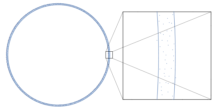
Figure 1. Eigenvalues of an induced Ginibre matrix in the almost-circular regime.

From the microscopic point of view, such almost-circular ensembles can be viewed as point processes mainly distributed on a strip. As this is a characteristic feature of almost-Hermitian random matrices [24] (or random normal matrices near a cusp type singularity [9]), one can expect from the general universality principles in random matrix theory that almost-circular ensembles lie in the same universality class previously appearing in these models. Furthermore, contrary to almost-Hermitian random matrices, where only a few specific models were analysed (see e.g. [3, 4, 12, 36, 1]), almost-circular ensembles provide concrete models allowing explicit asymptotic analysis possible.

In this note, we aim to derive various scaling limits of almost-circular ensembles, which give rise to further universality classes beyond the well-known deformed sine kernel introduced by Fyodorov, Khoruzhenko, and Sommers [25, 26, 24]. To be more precise, we shall consider the ensemble (1.2) with a general radially symmetric potential $Q_{n}$ and derive scaling limits under various boundary confinements.

Let us first introduce almost-circular ensembles. We consider a configuration $\{\zeta_{j}\}_{1}^{n}$ of points in $\mathbb{C}$ whose joint probability distribution ${\mathbf{P}}_{n}$ is of the form

(1.2) $$d\mathbf{P}_{n}=\frac{1}{Z_{n}}e^{-\mathbf{H}_{n}}\,dA_{n},\qquad\mathbf{H}_{n}:=\sum_{j>k}\log\frac{1}{|\zeta_{j}-\zeta_{k}|^{2}}+n\sum_{j=1}^{n}Q_{n}(\zeta_{j}),$$

where $dA_{n}:=(dA)^{\otimes n}$ is the normalised volume measure on $\mathbb{C}^{n}$ with $dA(\zeta)=\frac{1}{\pi}d^{2}\zeta$, and $Z_{n}$ is the partition function which turns $\mathbf{P}_{n}$ into a probability measure. Here, $Q_{n}:\mathbb{C}\to\mathbb{R}\cup\{\infty\}$ is a suitable function called external potential.

We remark that the induced Ginibre ensemble is associated with the potential

(1.3) $$Q_{n}^{I}(\zeta)=a_{n}|\zeta|^{2}-2b_{n}\log|\zeta|.$$

This is indeed a special case of a more general Mittag-Leffler potentials, see e.g. [16, 19, 11] and references therein. The Mittag-Leffler ensembles are contained in the class of models under consideration in this note.

Now we describe precise assumptions on the potentials $Q_{n}$. We begin with standard assumptions from the logarithmic potential theory [38]. By definition, the external potential $Q_{n}$ is a lower semicontinuous function which is finite on some set of positive capacity and satisfies

(1.4) $$\liminf_{\zeta\to\infty}\frac{Q_{n}(\zeta)}{2\log|\zeta|}\geq k,$$

where $k>1$ is a fixed constant independent of $n$. Then there exists a probability measure $\sigma_{Q_{n}}$ that minimises the energy functional

(1.5) $$I_{Q_{n}}[\mu]=\iint_{\mathbb{C}^{2}}\log\frac{1}{|\zeta-\eta|}\,d\mu(\zeta)\,d\mu(\eta)+\int_{\mathbb{C}}Q_{n}\,d\mu.$$

The support $S_{n}$ of the equilibrium measure $\sigma_{Q_{n}}$ is called the droplet, see e.g. [28]. It is also well known that if $\sigma_{Q_{n}}$ is absolutely continuous with respect to the area measure $dA$, the density on $S_{n}$ is $\Delta Q_{n}$, where $\Delta=\frac{1}{4}({\partial}_{x}^{2}+{\partial}_{y}^{2})$ is the quarter of the usual Laplacian.

Next, let us set the stage to investigate almost-circular ensembles. We consider a radially symmetric potential

(1.6) $$Q_{n}(\zeta)=g_{n}(r),\qquad r=|\zeta|,\qquad g_{n}:\mathbb{R}_{+}\to\mathbb{R},$$

where $g_{n}$ is $C^{3}$-differentiable on $\mathbb{R}_{+}$. Without loss of generality, we shall assume that $g_{n}(1)=0$ and $g_{n}^{\prime}(1)=1$. We also assume that $Q_{n}$ is subharmonic in $\mathbb{C}$ and strictly subharmonic in a neighbourhood of the unit circle. Then the associated droplet $S_{n}$ is given by the annulus

(1.7) $$S_{n}:=\{\zeta\in\mathbb{C}\,:\,r_{0}\leq|\zeta|\leq r_{1}\},$$

where $r_{0}\equiv r_{n,0}$ and $r_{1}\equiv r_{n,1}$ are the pair of constants satisfying

(1.8) $$r_{0}\,g_{n}^{\prime}(r_{0})=0,\qquad r_{1}\,g_{n}^{\prime}(r_{1})=2,$$

see [38, Section IV.6]. By (1.3) and (1.8), one can easily see that the droplet (1.1) of the induced Ginibre ensemble is a special case of (1.7).

We assume that $|g_{n}^{\prime\prime\prime}|\leq Cn$ in a neighbourhood of the unit circle for some constant $C$, and the limit

(1.9) $$\rho:=\lim_{n\to\infty}\sqrt{\frac{n}{\Delta Q_{n}(1)}}\in(0,\infty)$$

exists. Then it is easy to see that

(1.10) $$r_{0}=1-\frac{\rho^{2}}{4n}+o(n^{-1}),\qquad r_{1}=1+\frac{\rho^{2}}{4n}+o(n^{-1}).$$

This behaviour (1.10) makes the droplet (1.7) close to the unit circle. Furthermore, by (1.10), one can notice that the parameter $\rho$ defined by (1.9) plays the role in describing the width of the droplet, see [4] for more about the geometric meaning of such a parameter.

Now we introduce scaling limits of almost-circular ensembles. For this purpose, we denote by

(1.11) $$\mathbf{R}_{n,k}(\zeta_{1},\cdots,\zeta_{k}):=\frac{1}{Z_{n}}\frac{n!}{(n-k)!}\int_{\mathbb{C}^{n-k}}e^{-\mathbf{H}_{n}}\prod_{j=k+1}^{n}dA(\zeta_{j})$$

the $k$-point correlation function of model (1.2). In particular we write $\mathbf{R}_{n}\equiv\mathbf{R}_{n,1}$ for the $1$-point function. It is well known that $\{\zeta_{j}\}_{j=1}^{n}$ forms a determinantal point process [23, Chapter 5], namely, the $k$-point function (1.11) is expressed as

(1.12) $$\mathbf{R}_{n,k}(\zeta_{1},\cdots,\zeta_{k})=\det\Big{(}{\mathbf{K}}_{n}(\zeta_{j},\zeta_{l})\Big{)}_{j,l=1}^{k},$$

where a Hermitian function ${\mathbf{K}}_{n}$ is called a correlation kernel. Furthermore, ${\mathbf{K}}_{n}$ can be written in terms of the reproducing kernel for the space of analytic polynomials in $L^{2}(e^{-nQ_{n}})\,dA$:

(1.13) $${\mathbf{K}}_{n}(\zeta,\eta)=\sum_{j=0}^{n-1}p_{n,j}(\zeta)\overline{p_{n,j}(\eta)}e^{-\frac{n}{2}(Q_{n}(\zeta)+Q_{n}(\eta))},$$

where $p_{n,j}$ is the orthonormal polynomial of degree $j$ with respect to the measure $e^{-nQ_{n}}\,dA$. (We refer to [29] for a recent development of the theory of planar orthogonal polynomials.)

For the local investigation, we consider a zooming point $\alpha_{n}$ and define the rescaled ensemble $\{z_{j}\}_{1}^{n}$ by

(1.14) $$z_{j}:=\sqrt{n\Delta Q_{n}(\alpha_{n})}\cdot(\zeta_{j}-\alpha_{n}),$$

see Figure 1 for an illustration. Here, the specific choice of the rescaling factor $\sqrt{n\Delta Q_{n}(\alpha_{n})}$ follows from the mean eigenvalue spacing at the zooming point $\alpha_{n}.$ In the sequel, we frequently use the notation (1.14). We denote the $k$-point function $R_{n,k}$ of $\{z_{j}\}_{1}^{n}$ by

(1.15) $$R_{n,k}(z):=\frac{1}{(n\Delta Q_{n}(\alpha_{n}))^{k}}\mathbf{R}_{n,k}(\zeta),\qquad z=\sqrt{n\Delta Q_{n}(\alpha_{n})}\cdot(\zeta-\alpha_{n}).$$

By (1.12), one can observe that $R_{n,k}$ enjoys the determinatnal structure as well. In the sequel, we also write $R_{n}\equiv R_{n,1}.$

The following theorem is an immediate consequence of [4, Thoerem 3.8]. This approach is based on Ward’s equation, see Subsection 2.4 for more about this method.

Theorem 1.1.

Let $\alpha_{n}=1$. Then as $n\to\infty$, $R_{n}$ converges locally uniformly to the limit

(1.16) $$R^{(1)}(z)=\frac{1}{\sqrt{2\pi}}\int_{-\frac{\rho}{2}}^{\frac{\rho}{2}}e^{-\frac{1}{2}(2\operatorname{Re}z-\xi)^{2}}\,d\xi.$$

We emphasise that the scaling limit (1.16) agrees with the one appearing in the context of almost-Hermitan random matrices [25, 26, 24]. We also refer to [3, 4] and references therein for some known universality results in this class. (Cf. the symplectic version of Theorem 1.1 will appear in the forthcoming work [14].)

Note that we intentionally add the superscript $(1)$ in (1.16) since Theorem 1.1 can be realised as a special case of our results described in the following section. This will be clarified below. For the graph of $R^{(1)}$, see Figure 2 (A).

The limiting $1$-point function determines a unique determinantal point field, see [9, Lemma 1]. We also refer to [8, Theorem 1.1] and [4, Lemma 3.5] for the structure of a limiting correlation kernel of the rescaled system. To be more precise, for a class of potentials which are strictly subharmonic near the droplet, a limiting correlation kernel $K$ of a properly rescaled system is of the form

(1.17) $$K(z,w)=G(z,w)\cdot L(z,w),\qquad G(z,w)=e^{z\bar{w}-\frac{1}{2}|z|^{2}-\frac{1}{2}|w|^{2}},$$

where $L$ is Hermitian and analytic in $z$ and $\bar{w}$. Here $G$ is the Ginibre kernel, cf. [23]. Then as a consequence of (1.17), one can easily see the locally uniform convergence

(1.18) $$R_{n,k}\to\det\Big{(}K^{(1)}(z_{j},z_{l})\Big{)}_{j,l=1}^{k},\qquad K^{(1)}(z,w)=G(z,w)\,\frac{1}{\sqrt{2\pi}}\int_{-\frac{\rho}{2}}^{\frac{\rho}{2}}e^{-\frac{1}{2}(z+\bar{w}-\xi)^{2}}\,d\xi.$$

We remark that the kernel $K^{(1)}$ in (1.18) interpolates well-known Ginibre and sine kernels, see e.g. [3, Remark 4 (c)]. In the following section, we discuss several generalisations of Theorem 1.1.

2. Discussions of main results

In this section, we introduce our model and state main results. Throughout this note, we shall keep assumptions in Section 1 of the potential $Q_{n}$.

From now on, we refer to the situation in Theorem 1.1 where there is no boundary constraint as the free boundary or soft edge condition. On the other hand, if we completely confine the gas to the droplet $S_{n}$, we refer to this situation as the soft/hard edge condition. Equivalently, we redefine the potential $Q_{n}$ by setting $Q_{n}(\zeta)=+\infty$ when $\zeta\not\in S_{n}$. (See [9, 13, 15] and references therein for previous works studying such a boundary condition.) Indeed this terminology comes from its Hermitian counterpart, “soft edge meets hard edge” situation [20].

In [9], it was conjectured that for the random normal matrix ensemble in the strip with soft/hard edge condition, the limiting $1$-point function $R^{(\infty)}$ is of the form

(2.1) $$R^{(\infty)}(z)=\mathbf{1}_{\{|\operatorname{Re}z|<\frac{\rho}{4}\}}\cdot\int_{-\frac{\rho}{2}}^{\frac{\rho}{2}}\frac{e^{-\frac{1}{2}(2\operatorname{Re}z-\xi)^{2}}}{\int_{-\frac{\rho}{2}}^{\frac{\rho}{2}}e^{-\frac{1}{2}(t-\xi)^{2}}\,dt}\,d\xi.$$

(See Figure 2 (B) for the graph of $R^{(\infty)}$.) We also refer to [4, Subsection 8.3] for further supports of this conjecture.

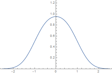
(a) free boundary

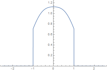
(b) soft/hard edge

Figure 2. The plots display graphs of $R^{(1)}(x)$ and $R^{(\infty)}(x)$ in (1.16) and (2.1), where $\rho=4$. The graphs are against the $x$-variable as they are invariant under translation in imaginary direction.

In this note, we address this problem for almost-circular ensembles. To our knowledge, Theorems 2.1 and 2.2 below provide the first concrete example of the scaling limits of the form (2.1). Therefore our results contribute to an affirmative answer for the conjecture in [9]. Furthermore, beyond the free and the soft/hard edge boundary conditions, we shall consider the following two natural boundary conditions which interpolate between these cases:

• Soft edge with a confinement parameter;

• Two-sided hard edge cuts.

The former one is a more potential theoretic boundary condition, whereas the latter one is a more geometric boundary condition.

The soft edge boundary condition with a confinement parameter is defined by a linear interpolation between the external potential $Q_{n}$ and the logarithmic potential of the equilibrium measure. We refer to [10] for potential theoretic motivations on such boundary conditions. See also [17, 27] for related boundary conditions. This convex combination gives rise to universal point fields which interpolate between the point fields with the $1$-point function (1.16) and with (2.1).

The two-sided hard edge boundary condition is obtained by moving the hard edge cuts that confine the gas to a narrow annulus between them. (We refer to [39, 30] for similar situations.) This boundary condition provides another interpolation between the $1$-point functions (1.16) and (2.1). In particular, by moving the hard edge cuts away from the droplet, one can recover the free boundary limit (1.16).

In the following subsections, we precisely introduce such boundary conditions and formulate our results.

2.1. Soft edge with a confinement parameter

First, let us discuss the soft edge with a confinement parameter. For this purpose, we consider the logarithmic potential

(2.2) $$U_{{Q_{n}}}(\zeta):=\int_{\mathbb{C}}\log\frac{1}{|\zeta-\eta|}\,d\sigma_{n}(\eta)$$

of $\sigma_{Q_{n}}$. Recall that $\sigma_{Q_{n}}$ is the equilibrium measure of the energy functional (1.5).

The obstacle function $\check{Q}_{n}$ pertaining to a potential $Q_{n}$ is defined by the maximal subharmonic function satisfying $\check{Q}_{n}\leq Q_{n}$ on $\mathbb{C}$ and $\check{Q}_{n}(\zeta)\leq\log|\zeta|^{2}+O(1)$ at infinity. Equivalently, it can be defined in terms of $U_{{Q_{n}}}$ in (2.2) as

(2.3) $$\check{Q}_{n}(\zeta)=C_{n}-2\,U_{Q_{n}}(\zeta),$$

where $C_{n}$ is the modified Robin constant, a unique constant satisfying $2U_{Q_{n}}+Q_{n}=C_{n}$ on $S_{n}$ and $2U_{Q_{n}}+Q_{n}\geq C_{n}$ on $\mathbb{C}$ (q.e.), see [38].

For a radially symmetric potential (1.6), the logarithmic potential $U_{{Q_{n}}}$ can be computed explicitly. As a consequence, the obstacle function $\check{Q}_{n}$ in (2.3) is given by

(2.4) $$\check{Q}_{n}(\zeta)=\begin{cases}Q_{n}(r_{0})&\text{if }|\zeta|<r_{0},\vskip 3.0pt plus 1.0pt minus 1.0pt\\ Q_{n}(\zeta)&\text{if }r_{0}\leq|\zeta|\leq r_{1},\vskip 3.0pt plus 1.0pt minus 1.0pt\\ 2\log|\zeta|-2\log r_{1}+Q_{n}(r_{1})&\text{otherwise},\end{cases}$$

see e.g. [10, 38]. (Recall that $r_{0}$ and $r_{1}$ are radii of the droplet $S_{n}$ in (1.7).) Using (2.4), for a given parameter $\mathbf{c}=(\mathbf{c}_{1},\mathbf{c}_{2})$ with $\mathbf{c}_{1},\mathbf{c}_{2}\in\mathbb{R}_{+}\cup\{\infty\}$, we define

(2.5) $$Q_{n}^{(\mathbf{c})}(\zeta):=\begin{cases}\mathbf{c}_{1}Q_{n}+(1-\mathbf{c}_{1})\check{Q}_{n}(\zeta)&\text{if }|\zeta|<r_{0},\vskip 3.0pt plus 1.0pt minus 1.0pt\\ Q_{n}(\zeta)&\text{if }r_{0}\leq|\zeta|\leq r_{1},\vskip 3.0pt plus 1.0pt minus 1.0pt\\ \mathbf{c}_{2}Q_{n}+(1-\mathbf{c}_{2})\check{Q}_{n}(\zeta)&\text{otherwise}.\end{cases}$$

Note that the parameter $\mathbf{c}_{1}$ (resp., $\mathbf{c}_{2}$) determines the boundary condition at inner (resp., outer) circle of the droplet.

To describe the scaling limits of almost-circular ensembles associated with the potential $Q_{n}^{(\mathbf{c})}$, let us write

(2.6) $$I^{(\mathbf{c})}(t):=\frac{1-\mathbf{c}_{1}}{2}\Big{(}t+\frac{\rho}{2}\Big{)}_{-}^{2}+\frac{1-\mathbf{c}_{2}}{2}\Big{(}t-\frac{\rho}{2}\Big{)}_{+}^{2}$$

and

(2.7) $$\Phi^{(\mathbf{c})}(\xi):=\int_{-\infty}^{\infty}e^{-\frac{1}{2}(t-\xi)^{2}+I^{(\mathbf{c})}(t)}\,dt.$$

(Here, we write $a_{+}=\max(a,0)$, $a_{-}=\min(a,0)$, and $a_{+}^{2}=(a_{+})^{2}$, $a_{-}^{2}=(a_{-})^{2}$ to avoid bulky notation.) These functions are building blocks to define

(2.8) $$F^{(\mathbf{c})}(z):=\int_{-\frac{\rho}{2}}^{\frac{\rho}{2}}\frac{e^{-\frac{1}{2}(z-\xi)^{2}}}{\Phi^{(\mathbf{c})}(\xi)}\,d\xi.$$

Let $\{\zeta_{j}\}_{1}^{n}$ be the particle system (1.2) in external potential $Q_{n}^{(\mathbf{c})}$ and $\{z_{j}\}_{1}^{n}$ be the rescaled system at $\alpha_{n}=1$, see (1.14). Notice that by (1.10), the point $\alpha_{n}=1$ is asymptotically the midpoint between $r_{0}$ and $r_{1}$. We write $R_{n}^{(\mathbf{c})}$ for the $1$-point function of the rescaled system.

We obtain the following result, which recovers Theorem 1.1 with the specific choice $\mathbf{c}_{1}=\mathbf{c}_{2}=1$.

Theorem 2.1.

(Scaling limits for the soft edge with a confinement parameter) As $n\to\infty$, the $1$-point function $R_{n}^{(\mathbf{c})}$ converges locally uniformly to the limit

(2.9) $$R^{(\mathbf{c})}(z)=F^{(\mathbf{c})}(2\operatorname{Re}z)\cdot\exp(I^{(\mathbf{c})}(2\operatorname{Re}z)),$$

where $F^{(\mathbf{c})}$ and $I^{(\mathbf{c})}$ are given by (2.8) and (2.6).

See Figure 3 for the graphs of $R^{(\mathbf{c})}$. We remark that the corresponding correlation kernel is given by

$$K^{(\mathbf{c})}(z,w)=G(z,w)\,F^{(\mathbf{c})}(z+\bar{w})\cdot\exp\Big{(}\frac{1}{2}I^{(\mathbf{c})}(2\operatorname{Re}z)+\frac{1}{2}I^{(\mathbf{c})}(2\operatorname{Re}w)\Big{)},$$

see [10, Theorem 1.1] for the structure of correlation kernels. It is easy to observe that in the extremal case $\mathbf{c}_{1}=\mathbf{c}_{2}=\infty$, the $1$-point function (2.9) corresponds to $R^{(\infty)}$ in (2.1) which appears in the soft/hard edge case. In this case, the limiting point field is strictly contained in the strip $\{z\in\mathbb{C}:|\operatorname{Re}z|<\frac{\rho}{4}\}$.

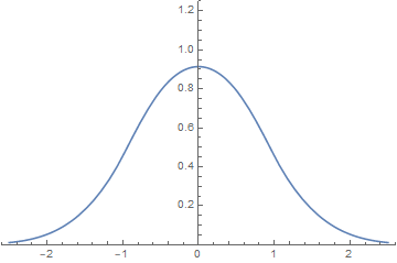
(a) $\mathbf{c}_{1}=\mathbf{c}_{2}=1/2$

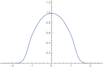
(b) $\mathbf{c}_{1}=\mathbf{c}_{2}=4$

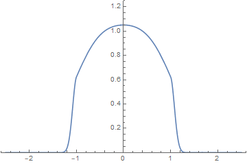
(c) $\mathbf{c}_{1}=\mathbf{c}_{2}=32$

Figure 3. The plots show graphs of $R^{(\mathbf{c})}(x)$ in (2.9) for a few values of $\mathbf{c}_{1}$ and $\mathbf{c}_{2}$, where $\rho=4$. One can observe that as $\mathbf{c}_{1},\mathbf{c}_{2}\to 1$, the graph of $R^{(\mathbf{c})}$ tends to $R^{(1)}$ in Figure 2 (A), whereas as $\mathbf{c}_{1},\mathbf{c}_{2}\to\infty$, it tends to $R^{(\infty)}$ in Figure 2 (B).

2.2. Hard edge confinements

We now consider the hard edge cuts near the droplet. For each $\tau\in\mathbb{R}$ with $0\leq\tau\leq 1$, there exists a unique number $r_{\tau}\equiv r_{n,\tau}$ such that

(2.10) $$r_{\tau}\,g_{n}^{\prime}(r_{\tau})=2\tau.$$

It is easy to observe from (2.10) that

(2.11) $$r_{\tau}=1-\frac{\rho^{2}}{4n}(1-2\tau)+o(n^{-1}),$$

see Lemma 3.1. Let us write

(2.12) $$S_{\tau}\equiv S_{n,\tau}:=\{\zeta\in\mathbb{C}:r_{0}\leq|\zeta|\leq r_{\tau}\},\qquad\Gamma_{\tau}\equiv\Gamma_{n,\tau}:=\{\zeta\in\mathbb{C}:|\zeta|=r_{\tau}\}.$$

We now consider the case where the hard edge cuts are along the circles $\Gamma_{\tau_{1}}$ and $\Gamma_{\tau_{2}}$ so that the particles are confined in the thin annulus

(2.13) $$S_{\tau_{2}}\setminus S_{\tau_{1}}=\{\zeta\in\mathbb{C}:r_{\tau_{1}}\leq|\zeta|\leq r_{\tau_{2}}\},\qquad(0\leq\tau_{1}<\tau_{2}\leq 1).$$

Equivalently, we consider the potential

(2.14) $$Q_{n}^{\tau_{1},\tau_{2}}(\zeta):=\begin{cases}Q_{n}(\zeta)&\text{if }r_{\tau_{1}}\leq|\zeta|\leq r_{\tau_{2}},\vskip 3.0pt plus 1.0pt minus 1.0pt\\ +\infty&\text{otherwise}.\end{cases}$$

In the presence of hard edge cuts, the associated equilibrium measure $\sigma_{Q_{n}}$ is no longer absolutely continuous with respect to the area measure $dA$ in general, and takes the form

(2.15) $$d\sigma_{Q_{n}}=\Delta Q\cdot\mathbf{1}_{S_{\tau_{2}}\setminus S_{\tau_{1}}}\,dA+\frac{\tau_{1}}{r_{\tau_{1}}}\mathbf{1}_{\Gamma_{\tau_{1}}}\,ds+\frac{1-\tau_{2}}{r_{\tau_{2}}}\mathbf{1}_{\Gamma_{\tau_{2}}}\,ds.$$

Here, $ds$ is the normalised arc length measure: $ds(z)=(2\pi)^{-1}|dz|$. One may realise from (2.15) that there are non-trivial portions of particles near the boundaries of (2.13).

More generally, for any real numbers $\tau_{1},\tau_{2}$ ($\tau_{1}<\tau_{2}$), one can define $r_{\tau_{1}}$, $r_{\tau_{2}}$, and $Q_{n}^{\tau_{1},\tau_{2}}$ when $n$ is sufficiently large. Note that when $\tau_{1}<0$ and $\tau_{2}>1$, the equilibrium measure associated with $Q^{\tau_{1},\tau_{2}}$ is not affected by the hard edge cuts.

We rescale the point process (1.2) associated with $Q_{n}^{\tau_{1},\tau_{2}}$ in (2.14) at the zooming point $\alpha_{n}=1$, i.e. $z_{j}=\sqrt{n\Delta Q_{n}(1)}(\zeta_{j}-1)$. We denote by $R_{n}^{\tau_{1},\tau_{2}}$ the $1$-point function of the rescaled system. Then we obtain the following theorem.

Theorem 2.2.

(Scaling limits for the two-sided hard edge cuts) As $n\to\infty$, the $1$-point function $R_{n}^{\tau_{1},\tau_{2}}$ converges locally uniformly to the limit

(2.16) $$R^{\tau_{1},\tau_{2}}(z)=\mathbf{1}_{\{\frac{\rho}{4}(2\tau_{1}-1)\leq x\leq\frac{\rho}{4}(2\tau_{2}-1)\}}\int_{-\rho/2}^{\rho/2}\frac{e^{-\frac{1}{2}(2x-\xi)^{2}}}{\int_{\frac{\rho}{2}(2\tau_{1}-1)}^{\frac{\rho}{2}(2\tau_{2}-1)}e^{-\frac{1}{2}(t-\xi)^{2}}\,dt}\,d\xi,\qquad x=\operatorname{Re}z.$$

See Figure 4 for the graphs of $R^{\tau_{1},\tau_{2}}$ with a few values of $\tau_{1}$ and $\tau_{2}$.

Note that the limiting point field of the rescaled system is completely confined in a strip which depends on the parameters $\tau_{1}$, $\tau_{2}$ of the hard edge cuts. By (1.17), it is easy to see that the correlation kernel associated with (2.16) is given by

(2.17) $$K^{\tau_{1},\tau_{2}}(z,w)=G(z,w)\,\int_{-\rho/2}^{\rho/2}\frac{e^{-\frac{1}{2}(z+\bar{w}-\xi)^{2}}}{\int_{\frac{\rho}{2}(2\tau_{1}-1)}^{\frac{\rho}{2}(2\tau_{2}-1)}e^{-\frac{1}{2}(t-\xi)^{2}}\,dt}\,d\xi$$

on the strip $\frac{\rho}{4}(2\tau_{1}-1)\leq\operatorname{Re}z,\operatorname{Re}w\leq\frac{\rho}{4}(2\tau_{2}-1)$, see e.g. [9, 4]. We remark that in [34], the authors considered another notion of hard edge cuts, which yield different scaling limits.

Notice that in the extremal case when $\tau_{1}=-\infty$ and $\tau_{2}=\infty$, the limiting $1$-point function $R^{\tau_{1},\tau_{2}}$ corresponds to (1.16), which appears in the free boundary case. On the other hand, if $\tau_{1}=0$ and $\tau_{2}=1$, it correspond to (2.1), which appears in the soft/hard edge case.

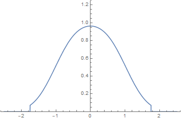
(a) $\tau_{1}=-\frac{3}{8}$, $\tau_{2}=\frac{11}{8}$

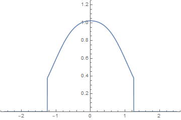
(b) $\tau_{1}=-\frac{1}{8}$, $\tau_{2}=\frac{9}{8}$

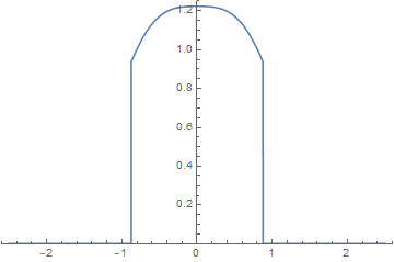
(c) $\tau_{1}=\frac{1}{16}$, $\tau_{2}=\frac{15}{16}$

Figure 4. The plots indicate graphs of $R^{\tau_{1},\tau_{2}}(x)$ in (2.16), where $\rho=4$. One can easily observe that as $\tau_{1}\to-\infty$ and $\tau_{2}\to\infty$, the graph of $R^{\tau_{1},\tau_{2}}$ tends to $R^{(1)}$ in Figure 2 (A). On the other hand, as $\tau_{1}\to 0$ and $\tau_{2}\to 1$, it tends to $R^{(\infty)}$ in Figure 2 (B).

Remark.

(Circular limit $\rho\to 0$) In the limit when $\rho\to 0$, one can recover the well-known sine kernel appearing in the circular unitary ensemble, see e.g. [23]. To take such a limit, we rescale the kernel via $z\mapsto z/a$ with $a=\rho/2$. (This is due to the fact that we have kept the “two-dimensional” perspective, see e.g. [4] for more details.) The associated kernel $\widetilde{K}^{\tau_{1},\tau_{2}}$ is given by

(2.18) $$\widetilde{K}^{\tau_{1},\tau_{2}}(z,w):=\frac{1}{a^{2}}K^{\tau_{1},\tau_{2}}(\frac{z}{a},\frac{w}{a}),\qquad\frac{\rho^{2}}{8}(2\tau_{1}-1)\leq\operatorname{Re}z,\operatorname{Re}w\leq\frac{\rho^{2}}{8}(2\tau_{2}-1).$$

Then it is easy to see that up to a cocycle, one can recover the sine kernel in the circular limit, i.e.

(2.19) $$\lim_{a\to 0}\widetilde{K}^{\tau_{1},\tau_{2}}(z,w)=\frac{1}{\pi}\frac{\sin(u-v)}{u-v},\qquad\begin{cases}u=\operatorname{Im}z,\vskip 3.0pt plus 1.0pt minus 1.0pt\\ v=\operatorname{Im}w.\end{cases}$$

See Subsection 3.2 for further details.

As a special case, let us consider the one-sided hard edge case that the hard edge is along the outer circle $\Gamma_{\tau_{2}}$ but the inner one $\Gamma_{\tau_{1}}$ is a free boundary, i.e. $\tau_{1}=-\infty$ and $\tau_{2}=\tau$, cf. (2.11) and (2.12). This model corresponds to the external potential

(2.20) $$Q_{n}^{\tau}(\zeta):=\begin{cases}Q_{n}(\zeta)&\text{if }|\zeta|\leq r_{\tau},\vskip 3.0pt plus 1.0pt minus 1.0pt\\ +\infty&\text{otherwise}.\end{cases}$$

We rescale the point process associated with the potential $Q_{n}^{\tau}$ in (2.20) at a point $r_{\tau}$ on the outer circle, i.e. $z_{j}=\sqrt{n\Delta Q_{n}(1)}(\zeta_{j}-r_{\tau})$ and denote by $R_{n}^{\tau}$ the $1$-point function of the rescaled system.

Corollary 2.3.

(Scaling limits for the one-sided hard edge cuts) As $n\to\infty$, the $1$-point function $R_{n}^{\tau}$ converges locally uniformly to the limit

(2.21) $$R^{\tau}(z)=\mathbf{1}_{\{x\leq 0\}}\int_{-\rho\tau}^{\rho(1-\tau)}\frac{e^{-\frac{1}{2}(2x-\xi)^{2}}}{\int_{-\infty}^{0}e^{-\frac{1}{2}(t-\xi)^{2}}\,dt}\,d\xi,\qquad x=\operatorname{Re}z.$$

In particular, the rescaled $1$-point function

(2.22) $$\widetilde{R}^{\tau}(z):=\Big{(}\frac{c(\tau)}{\rho}\Big{)}^{2}R^{\tau}\Big{(}\frac{c(\tau)}{\rho}z\Big{)},\qquad c(\tau):=\Big{(}\sqrt{\frac{(1-\tau)^{2}}{4}+\frac{1}{\rho^{2}}}+\frac{1-\tau}{2}\Big{)}^{-1}$$

satisfies

(2.23) $$\lim_{\rho\to\infty}\widetilde{R}^{\tau}(z)=\begin{cases}\displaystyle\mathbf{1}_{\{x\leq 0\}}\int_{-\infty}^{0}\frac{e^{-\frac{1}{2}(x-\xi)^{2}}}{\int_{-\infty}^{0}e^{-\frac{1}{2}(t-\xi)^{2}}\,dt}\,d\xi,&\text{if }\tau=1,\vskip 3.0pt plus 1.0pt minus 1.0pt\\ \displaystyle\mathbf{1}_{\{x\leq 0\}}\int_{0}^{1}\xi\cdot e^{2x\xi}\,d\xi,&\text{if }\tau\in(0,1).\end{cases}$$

See Figure 5 for the graphs of $R^{\tau}(x)$.

We emphasise that in (2.23), the former limit corresponds to the $1$-point function for the soft/hard edge Ginibre ensemble [23, 8], whereas the latter one corresponds to the $1$-point function for hard edge Ginibre ensemble [39]. Moreover, the latter limit also appears in the context of truncated unitary ensembles [41, 32].

Let us briefly explain the rescaling factor $c(\tau)$ in (2.22). The $1$-point function $\widetilde{R}^{\tau}$ appears when we rescale the point process as $z_{j}=\gamma_{n}(\zeta_{j}-r_{\tau})$, where $\gamma_{n}$ satisfies

(2.24) $$\Delta Q(p)\,\gamma_{n}^{2}+\frac{1-\tau}{r_{\tau}}\,\gamma_{n}=\frac{1}{n}.$$

Note that by (2.15), the constant $\gamma_{n}$ corresponds to the mean eigenvalue spacing at $r_{\tau}$. Then the rescaling (2.22) follows from (2.24) since $\gamma_{n}\asymp c(\tau)/n$.

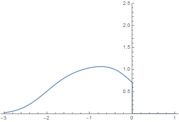
(a) $\tau=1$

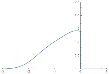
(b) $\tau=\frac{5}{6}$

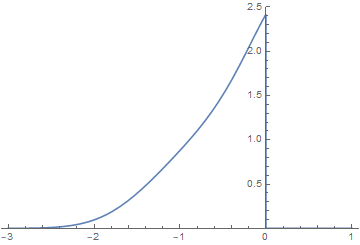
(c) $\tau=\frac{2}{3}$

Figure 5. The graphs of $R^{\tau}(x)$ in (2.21). Here $\rho=4$.

2.3. Maximal and minimal modulus

In our final main result, we study the maximal and minimal modulus of almost-circular ensembles associated with the potential (2.5).

For the system $\{\zeta_{j}\}_{j=1}^{n}$ in (1.2) with the potential (2.5), we consider its maximal and minimal modulus

(2.25) $$|\zeta|_{n}:=\max_{1\leq j\leq n}|\zeta_{j}|,\qquad|\zeta|_{1}:=\min_{1\leq j\leq n}|\zeta_{j}|.$$

This notation (2.25) will be used in the sequel. To investigate the fluctuation of the maximal (resp., minimal) modulus, we rescale $|\zeta|_{n}$ (resp., $|\zeta|_{1}$) near the outer (resp., inner) boundary of the droplet.

Here, we should distinguish the soft/hard edge case. Accordingly, we define random variables $\omega_{n}$ and $u_{n}$ as follows.

• If $\mathbf{c}_{1},\mathbf{c}_{2}<\infty$,

  (2.26) $$\omega_{n}:=a_{n}(|\zeta|_{n}-b_{n}),\qquad u_{n}:=a_{n}^{\prime}(b_{n}^{\prime}-|\zeta|_{1}),$$

  where

  (2.27) $$\begin{split}a_{n}&=\frac{2n}{\rho}\sqrt{\mathbf{c}_{2}\,c_{n}},\qquad b_{n}=r_{1}+\frac{\rho}{2n}\sqrt{\frac{c_{n}}{\mathbf{c}_{2}}},\\ a_{n}^{\prime}&=\frac{2n}{\rho}\sqrt{\mathbf{c}_{1}\,c_{n}^{\prime}},\qquad b_{n}^{\prime}=r_{0}-\frac{\rho}{2n}\sqrt{\frac{c_{n}^{\prime}}{\mathbf{c}_{1}}}.\end{split}$$

  Here

  (2.28) $$\begin{split}c_{n}&=2\log\frac{n}{\rho}-2\log\log n-2\log\big{(}2\,\Phi^{(\mathbf{c})}(\frac{\rho}{2})\big{)},\\ c_{n}^{\prime}&=2\log\frac{n}{\rho}-2\log\log n-2\log\big{(}2\,\Phi^{(\mathbf{c})}(-\frac{\rho}{2})\big{)}.\end{split}$$

• If $\mathbf{c}_{1}=\mathbf{c}_{2}=\infty$,

  (2.29) $$\omega_{n}:=\frac{c\,n^{2}}{\rho^{2}}(|\zeta|_{n}-r_{1}),\qquad u_{n}:=\frac{c^{\prime}\,n^{2}}{\rho^{2}}(r_{0}-|\zeta|_{1}),$$

  where

  (2.30) $$c=2R^{(\infty)}(\frac{\rho}{4}),\qquad c^{\prime}=2R^{(\infty)}(-\frac{\rho}{4}).$$

Here, $\Phi^{(\mathbf{c})}$ and $R^{(\infty)}$ are given in (2.7) and (2.1) respectively. We remark that the specific choice of parameters (2.27), (2.28), and (2.30) leads to the universal form of the distributions (2.31), (2.32) below. We obtain the following theorem.

Theorem 2.4.

(Fluctuations of the maximal and minimal modulus) The followings hold.

1. If $\mathbf{c}_{1},\mathbf{c}_{2}<\infty$, the random variables $\omega_{n}$ and $u_{n}$ in (2.26) converge in distribution to the standard Gumbel distribution, i.e.

   (2.31) $$\lim_{n\to\infty}{\mathbf{P}}_{n}(\omega_{n}\leq x)=\lim_{n\to\infty}{\mathbf{P}}_{n}(u_{n}\leq x)=e^{-e^{-x}},\qquad x\in\mathbb{R}.$$

2. If $\mathbf{c}_{1}=\mathbf{c}_{2}=\infty$, the random variables $\omega_{n}$ and $u_{n}$ in (2.29) converge in distribution to the standard exponential distribution, i.e.

   (2.32) $$\lim_{n\to\infty}{\mathbf{P}}_{n}(\omega_{n}\leq x)=\lim_{n\to\infty}{\mathbf{P}}_{n}(u_{n}\leq x)=e^{x},\qquad x\in\mathbb{R}_{-}.$$

This theorem asserts that the fluctuations of maximal and minimal modulus are same as those previously obtained for the usual random normal matrices [18, 33, 37, 40] (and also planar symplectic ensembles [37, 21]). In other words, the distributions (2.31) and (2.32) universally appear also in the context of almost-circular ensembles.

2.4. Remarks on main theorems and glimpses of Ward’s equations

We end this section by giving some general remarks and briefly introducing alternative approach based on Ward’s equations.

The overall strategy for the proofs of our main theorems are as follows. Using the exact solvability of the model, we express the correlation kernel in terms of the orthonormal polynomials with respect to the weighted Lebesgue measure $e^{-nQ_{n}}\,dA,$ see (1.13). Since the external potential $Q_{n}$ is radially symmetric, the orthonormal polynomial is a monomial. The asymptotics of the leading coefficient of such a polynomial can be obtained by virtue of Laplace methods, which allows us to derive large-$n$ limits of the correlation kernel by a proper Riemann sum approximation.

Our proofs for the scaling limits (Theorems 2.1 and  2.2) are completely different with those used in [4] for Theorem 1.1. In general, it can be shown that the limiting $1$-point function $R$ satisfies certain partial integro-differential equation called Ward’s equation. For the free boundary condition, it is of the form

(2.33) $$\partial C(z)=R(z)-1-\Delta\log R(z),\qquad C(z):=\frac{1}{R(z)}\int_{\mathbb{C}}\frac{|K(z,w)|^{2}}{z-w}\,dA(w).$$

An important feature of this equation is that it does not depend on the choice of the external potential.

In [4], the notion of “cross-section convergence” for general bandlimited point processes was introduced. Combining this property with the characterisation of translation invariant solutions to Ward’s equation (obtained in [9]), the authors derived various scaling limits of almost-Hermitian type ensembles under some natural geometric conditions notably the translation invariance of scaling limits. In particular, since such conditions trivially hold for almost-circular ensembles, this immediately leads to Theorem 1.1. (We refer the reader to [2, Remark 2.9] for a summary of the approach using Ward’s equation in the study of universality.)

We briefly present Ward’s equations in our various cases ($R^{(\mathbf{c})}$ in (2.9); $R^{\tau_{1},\tau_{2}}$ in (2.16); $R^{\tau}$ in (2.21); $\widetilde{R}^{\tau}$ in (2.22)) and compare them with those in previous literature. In the spirit of [4, 9, 8], this may be used to study the existence of further universality classes beyond radially symmetric ensembles. We also refer to [31] and [2] for implementations of Ward’s equations in the study of Hermitian random matrices and planar symplectic ensembles respectively. We remark that for a general class of external potentials, the local bulk and edge universality of random normal matrices were obtained in [6] and [29] respectively. (See also a recent work [5] which establishes Szegő type asysmptotics for the correlation kernel.)

The derivation of Ward’s equations follows from the standard method found for instance in [8, 7] and we skip the proof. The main idea is the reparametrisation invariance of the partition function $Z_{n}$.

In each situation, we write $C^{(\mathbf{c})}$, $C^{\tau_{1},\tau_{2}}$, $C^{\tau}$ and $\widetilde{C}^{\tau}$ for the associated Cauchy transforms of the form (2.33).

• Ward’s equation for soft edge with a confinement parameter. The $1$-point function $R^{(\mathbf{c})}$ in (2.9) satisfies

  (2.34) $${\bar{\partial}}C^{(\mathbf{c})}(z)=R^{(\mathbf{c})}(z)-1-\Delta\log R^{(\mathbf{c})}(z)+(1-\mathbf{c}_{1})\mathbf{1}_{\operatorname{Re}z<-\frac{\rho}{4}}+(1-\mathbf{c}_{2})\mathbf{1}_{\operatorname{Re}z>\frac{\rho}{4}}.$$

  We remark that if $\mathbf{c}_{1}=1$ or $\mathbf{c}_{2}=1$, the equation (2.34) corresponds to the one presented in [10, Theorem 1.1]. Furthermore, if $\mathbf{c}_{1}=\mathbf{c}_{2}=1$, then (2.34) corresponds to (2.33).

• Ward’s equation for two-sided hard edge. The $1$-point function $R^{\tau_{1},\tau_{2}}$ in (2.16) satisfies

  (2.35) $${\bar{\partial}}C^{\tau_{1},\tau_{2}}(z)=R^{\tau_{1},\tau_{2}}(z)-1-\Delta\log R^{\tau_{1},\tau_{2}}(z),\qquad\frac{\rho}{4}(2\tau_{1}-1)\leq\operatorname{Re}z\leq\frac{\rho}{4}(2\tau_{2}-1).$$

  Such form of Ward’s equation was extensively studied in [9]. Notice that if $\tau_{1}\to-\infty$ and $\tau_{2}\to\infty$, then (2.35) corresponds to (2.33).

• Ward’s equation for one-sided hard edge. The $1$-point function $R^{\tau}$ in (2.21) satisfies

  (2.36) $${\bar{\partial}}C^{\tau}(z)=R^{\tau}(z)-1-\Delta\log R^{\tau}(z),\qquad\operatorname{Re}z\leq 0.$$

  The equation (2.36) corresponds to the one presented in [8, Subsection 7.1]. By the change of variable, it is easy to see that the $1$-point function $\widetilde{R}^{\tau}$ in (2.22) satisfies

  (2.37) $${\bar{\partial}}\widetilde{C}^{\tau}(z)=\widetilde{R}^{\tau}(z)-(\frac{c(\tau)}{\rho})^{2}-\Delta\log\widetilde{R}^{\tau}(z),\qquad\operatorname{Re}z\leq 0.$$

  Note that if $0<\tau<1$, we have $c(\tau)/\rho\to 0$ as $\rho\to\infty$. Therefore by taking the limit $\rho\to\infty$ of (2.37), we arrive at

  (2.38) $${\bar{\partial}}\widetilde{C}^{\tau}(z)=\widetilde{R}^{\tau}(z)-\Delta\log\widetilde{R}^{\tau}(z),\qquad\operatorname{Re}z\leq 0,\qquad(\rho=\infty).$$

  This form (2.38) of Ward’s equation was used in [39] to study scaling limits of hard edge ensembles.

The rest of this note is structured as follows. In Section 3, we derive various scaling limits (Theorems 2.1,  2.2 and Corollary 2.3). Section 4 is devoted to the study of maximal and minimal modulus of the ensemble, Theorem 2.4.

3. Scaling limits of almost-circular ensembles

In this section, we show Theorems 2.1,  2.2 and Corollary 2.3.

3.1. Soft edge with a confinement parameter

In this subsection, we prove Theorem 2.1.

Recall that for each real $\tau$, $r_{\tau}=r_{n,\tau}$ denotes a unique constant satisfying (2.10). The following lemma gives the asymptotic expansion of $r_{\tau}$.

Lemma 3.1.

For each fixed $\tau$, we have

(3.1) $$r_{\tau}=1-\frac{\rho^{2}}{4n}(1-2\tau)+o(n^{-1}),\qquad n\to\infty.$$

Proof.

Since $g_{n}(1)=0$ and $g_{n}^{\prime}(1)=1$, we have $r_{\tau}=1$ when $\tau=\frac{1}{2}$. By Taylor series expansion, it follows from (1.9) that

$$1-2\tau =g_{n}^{\prime}(1)-r_{\tau}g_{n}^{\prime}(r_{\tau})=\frac{d}{dr}(rg^{\prime}(r))|_{r=1}\cdot(1-r_{\tau})\cdot(1+o(1))$$

$$=4\Delta Q_{n}(1)\cdot(1-r_{\tau})\cdot(1+o(1))=\frac{4n}{\rho^{2}}\cdot(1-r_{\tau})\cdot(1+o(1)),$$

which completes the proof. ∎

Let us write

(3.2) $$\delta_{n}=n^{-1}\log n.$$

By (2.4), it is easy to observe that for $r_{0}-\delta_{n}<r<r_{0}$,

(3.3) $$(Q_{n}-\check{Q}_{n})(r)=2\Delta Q_{n}(r_{0})(r-r_{0})^{2}+O(n|r-r_{0}|^{3})=\frac{2n}{\rho^{2}}(r-r_{0})^{2}\cdot(1+o(1))+O(n\delta_{n}^{3})$$

as $n\to\infty$. Similarly, for $r_{1}<r<r_{1}+\delta_{n}$,

(3.4) $$(Q_{n}-\check{Q}_{n})(r)=2\Delta Q_{n}(r_{1})(r-r_{1})^{2}+O(n|r-r_{1}|^{3})=\frac{2n}{\rho^{2}}(r-r_{1})^{2}\cdot(1+o(1))+O(n\delta_{n}^{3}).$$

We first prove some estimates for the $L^{2}$-norm of monomials with respect to the measure $e^{-nQ_{n}^{(\mathbf{c})}}\,dA$.

For each $j$ with $0\leq j\leq n-1$, we define the functions $v_{n,j}$ by

(3.5) $$v_{n,j}(r)=g_{n}(r)-2\tau(j)\log r,\qquad\tau(j):=j/n.$$

The function $v_{n,j}$ has a unique critical point at $r_{\tau(j)}$. We obtain the expansion

(3.6) $$\begin{split}v_{n,j}(r)&=v_{n,j}(r_{\tau(j)})+2\Delta Q(r_{\tau(j)})(r-r_{\tau(j)})^{2}+O(n\delta_{n}^{3})\\ &=v_{n,j}(r_{\tau(j)})+\frac{2n}{\rho^{2}}(r-r_{\tau(j)})^{2}\cdot(1+o(1))+O(n\delta_{n}^{3})\end{split}$$

for all $r$ with $|r-r_{\tau(j)}|\leq\delta_{n}$. Recall that $\Phi^{(\mathbf{c})}$ is given by (2.7).

We write

(3.7) $$\|\zeta^{j}\|_{nQ_{n}^{(\mathbf{c})}}^{2}:=\int_{\mathbb{C}}|\zeta^{j}|^{2}e^{-nQ_{n}^{(\mathbf{c})}(\zeta)}\,dA(\zeta)$$

for the orthogonal norm. Then we obtain the following asymptotic behaviour of (3.7).

Lemma 3.2.

For each $j$ with $0\leq j\leq n$, we have

(3.8) $$\|\zeta^{j}\|_{nQ_{n}^{(\mathbf{c})}}^{2}=e^{-nv_{n,j}(r_{\tau(j)})}\frac{\rho}{n}\,\Phi^{(\mathbf{c})}\Big{(}\rho(\tau(j)-\frac{1}{2})\Big{)}\cdot(1+o(1)),$$

where $\tau(j)=j/n$ and $o(1)\to 0$ uniformly in $j$.

Proof.

In order to evaluate (3.7), we split the integral into the sum of three integrals:

$$\|\zeta^{j}\|_{nQ_{n}^{(\mathbf{c})}}^{2} =\int_{S_{n}}|\zeta^{j}|^{2}e^{-nQ_{n}(\zeta)}\,dA(\zeta)$$

$$\quad+\int_{|\zeta|<r_{0}}|\zeta^{j}|^{2}e^{-nQ_{n}^{(\mathbf{c})}(\zeta)}\,dA(\zeta)+\int_{|\zeta|>r_{1}}|\zeta^{j}|^{2}e^{-nQ_{n}^{(\mathbf{c})}(\zeta)}\,dA(\zeta),$$

where $S_{n}$ is given by (1.7). By (3.6), the standard Laplace’s method gives rise to

$$\int_{S_{n}}|\zeta^{j}|^{2}e^{-nQ_{n}(\zeta)}\,dA(\zeta) =\int_{r_{0}}^{r_{1}}e^{-nv_{n,j}(r)}\,2r\,dr$$

$$=e^{-nv_{n,j}(r_{\tau(j)})}\!\!\int_{r_{0}}^{r_{1}}e^{-\frac{2n^{2}}{\rho^{2}}(r-r_{\tau(j)})^{2}}\,2\,dr\cdot(1+o(1))$$

$$=e^{-nv_{n,j}(r_{\tau(j)})}\!\!\int_{-\frac{\rho}{2}}^{\frac{\rho}{2}}e^{-\frac{1}{2}(t-\rho(\tau(j)-\frac{1}{2}))^{2}}\frac{\rho}{n}\,dt\cdot(1+o(1)),$$

where we use Lemma 3.1 and make the change of variable $t=\frac{2n}{\rho}(r-1)$. In the same way, we obtain from the asymptotic expansions (3.3), (3.4), and (3.6) that

$$\int_{|\zeta|<r_{0}}\!\!\!|\zeta^{j}|^{2}e^{-nQ_{n}^{(\mathbf{c})}(\zeta)}\,dA(\zeta) =\int_{0}^{r_{0}}e^{-n(v_{n,j}(r)-(1-\mathbf{c}_{1})(Q_{n}-\check{Q}_{n})(r))}\,2r\,dr$$

$$=e^{-nv_{n,j}(r_{\tau(j)})}\!\!\int_{r_{0}-\delta_{n}}^{r_{0}}e^{-\frac{2n^{2}}{\rho^{2}}((r-r_{\tau(j)})^{2}-(1-\mathbf{c}_{1})(r-r_{0})^{2})}\,2\,dr\cdot(1+o(1))$$

$$=e^{-nv_{n,j}(r_{\tau(j)})}\!\!\int_{-\infty}^{-\frac{\rho}{2}}\!e^{-\frac{1}{2}((t-\rho(\tau(j)-\frac{1}{2}))^{2}-(1-\mathbf{c}_{1})(t+\frac{\rho}{2})^{2})}\frac{\rho}{n}\,dt\cdot(1+o(1))$$

and

$$\int_{|\zeta|>r_{1}}\!\!\!|\zeta^{j}|^{2}e^{-nQ_{n}^{(\mathbf{c})}(\zeta)}\,dA(\zeta) =\int_{r_{1}}^{\infty}e^{-n(v_{n,j}(r)-(1-\mathbf{c}_{2})(Q_{n}-\check{Q}_{n})(r))}\,2r\,dr$$

$$=e^{-nv_{n,j}(r_{\tau(j)})}\!\!\int_{r_{1}}^{r_{1}+\delta_{n}}e^{-\frac{2n^{2}}{\rho^{2}}((r-r_{\tau(j)})^{2}-(1-\mathbf{c}_{2})(r-r_{1})^{2})}\,2\,dr\cdot(1+o(1))$$

$$=e^{-nv_{n,j}(r_{\tau(j)})}\!\!\int_{\frac{\rho}{2}}^{\infty}\!e^{-\frac{1}{2}((t-\rho(\tau(j)-\frac{1}{2}))^{2}-(1-\mathbf{c}_{2})(t-\frac{\rho}{2})^{2})}\frac{\rho}{n}\,dt\cdot(1+o(1)).$$

Combining all of the above, we conclude (3.8). ∎

We now prove Theorem 2.1.

Proof of Theorem 2.1.

By (1.12), (1.13), and (1.15), the $1$-point function $R_{n}^{(\mathbf{c})}$ rescaled at $\alpha_{n}=1$ is written as

(3.9) $$R_{n}^{(\mathbf{c})}(z)=\frac{1}{n\Delta Q_{n}(1)}\sum_{j=0}^{n-1}\frac{|\zeta^{j}|^{2}}{\|\zeta^{j}\|_{nQ_{n}^{(\mathbf{c})}}^{2}}e^{-nQ_{n}^{(\mathbf{c})}(\zeta)},\qquad\zeta=1+\frac{z}{\sqrt{n\Delta Q(1)}}.$$

We shall analyse the asymptotic behaviour of (3.9).

Fix a compact subset ${\mathcal{K}}$ in $\mathbb{C}$. For $\zeta=1+z/\sqrt{n\Delta Q_{n}(1)}$ with $r_{0}\leq|\zeta|\leq r_{1}$ and $z\in{\mathcal{K}}$, it follows from the expansion (3.6) that

$$Q_{n}^{(\mathbf{c})}(\zeta)-2\tau(j)\log|\zeta| =v_{n,j}(r_{\tau(j)})+\frac{2n}{\rho^{2}}\Big{(}1+\frac{x}{\sqrt{n\Delta Q_{n}(1)}}-r_{\tau(j)}\Big{)}^{2}\cdot(1+o(1))$$

$$=v_{n,j}(r_{\tau(j)})+\frac{1}{2n}\Big{(}2x-\rho(\tau(j)-\frac{1}{2})\Big{)}^{2}\cdot(1+o(1)),$$

where $\tau(j)=j/n$ and $x=\operatorname{Re}z$. Similarly, for $|\zeta|<r_{0}$ and $z\in{\mathcal{K}}$, we have

$$Q_{n}^{(\mathbf{c})}(\zeta)-2\tau(j)\log|\zeta| =v_{n,j}(\zeta)-(1-\mathbf{c}_{1})(Q-\check{Q})(\zeta)$$

$$=v_{n,j}(r_{\tau(j)})+\frac{1}{2n}\Big{(}(2x-\rho(\tau(j)-\frac{1}{2}))^{2}-(1-\mathbf{c}_{1})(2x+\frac{\rho}{2})^{2}\Big{)}\cdot(1+o(1)).$$

Finally, for $|\zeta|>r_{1}$ and $z\in{\mathcal{K}}$, we have

$$Q_{n}^{(\mathbf{c})}(\zeta)-2\tau(j)\log|\zeta| =v_{n,j}(\zeta)-(1-\mathbf{c}_{2})(Q-\check{Q})(\zeta)$$

$$=v_{n,j}(r_{\tau(j)})+\frac{1}{2n}\Big{(}(2x-\rho(\tau(j)-\frac{1}{2}))^{2}-(1-\mathbf{c}_{2})(2x-\frac{\rho}{2})^{2}\Big{)}\cdot(1+o(1)).$$

Here, the $o(1)$-terms are bounded uniformly for all $j$ with $0\leq j\leq n-1$ and all $z\in{\mathcal{K}}$.

Combining all of the above with Lemma 3.2, we obtain the following Riemann sum approximation of (3.9):

$$R_{n}^{(\mathbf{c})}(z) =\sum_{j=0}^{n-1}\frac{\rho\,e^{-\frac{1}{2}(2x-\rho(\tau(j)-\frac{1}{2}))^{2}}}{n\Phi^{(\mathbf{c})}(\rho(\tau(j)-\frac{1}{2}))}e^{\frac{1-\mathbf{c}_{1}}{2}(2x+\frac{\rho}{2})^{2}\cdot\mathbf{1}_{\{x<-\frac{\rho}{4}\}}+\frac{1-\mathbf{c}_{2}}{2}(2x-\frac{\rho}{2})^{2}\cdot\mathbf{1}_{\{x>\frac{\rho}{4}\}}}\cdot(1+o(1))$$

$$=\int_{-\frac{\rho}{2}}^{\frac{\rho}{2}}\frac{e^{-\frac{1}{2}(2x-\xi)^{2}}}{\Phi^{(\mathbf{c})}(\xi)}d\xi\cdot e^{\frac{1-\mathbf{c}_{1}}{2}(2x+\frac{\rho}{2})^{2}\cdot\mathbf{1}_{\{x<-\frac{\rho}{4}\}}+\frac{1-\mathbf{c}_{2}}{2}(2x-\frac{\rho}{2})^{2}\cdot\mathbf{1}_{\{x>\frac{\rho}{4}\}}}\cdot(1+o(1)),$$

where $o(1)\to 0$ uniformly for $z\in{\mathcal{K}}$ as $n\to\infty$. This completes the proof. ∎

3.2. Hard edge case

In this subsection, we prove Theorem 2.2. The strategy is similar to the one in the previous subsection.

Proof of Theorem 2.2.

Again we need to analyse the orthogonal norm

(3.10) $$\|\zeta^{j}\|^{2}_{nQ_{n}^{\tau_{1},\tau_{2}}}:=\int_{S_{\tau_{2}}\setminus S_{\tau_{1}}}|\zeta|^{2j}e^{-nQ_{n}(\zeta)}\,dA(\zeta)=\int_{r_{\tau_{1}}}^{r_{\tau_{2}}}e^{-nv_{n,j}(r)}\,2r\,dr$$

associated with the potential (2.14). Here $v_{n,j}(r)=g_{n}(r)-\frac{2j}{n}\log r$, cf. (1.6). By the Taylor series expansion, with $\tau(j)=j/n$, we have

$$v_{n,j}(r)=v_{n,j}(r_{\tau(j)})+\frac{2n}{\rho^{2}}(r-r_{\tau(j)})^{2}\cdot(1+o(1))+O(n|r-r_{\tau(j)}|^{3}).$$

As in Lemma 3.8, the $L^{2}$-norm (3.10) is approximated by

(3.11) $$\begin{split}\|\zeta^{j}\|^{2}_{nQ_{n}^{\tau_{1},\tau_{2}}}&=e^{-nv_{n,j}(r_{\tau(j)})}\int_{r_{\tau_{1}}}^{r_{\tau_{2}}}e^{-\frac{2n^{2}}{\rho^{2}}(r-r_{\tau(j)})^{2}}\,2\,dr\cdot(1+o(1))\\ &=e^{-nv_{n,j}(r_{\tau(j)})}\frac{\rho}{n}\int_{\frac{\rho}{2}(2\tau_{1}-1)}^{\frac{\rho}{2}(2\tau_{2}-1)}e^{-\frac{1}{2}(t-\frac{\rho}{2}(2\tau(j)-1))^{2}}\,dt\cdot(1+o(1)).\end{split}$$

Note that by (1.12), (1.13), and (1.15), the $1$-point function $R_{n}^{\tau_{1},\tau_{2}}$ associated with the hard edge potential (2.14) is written as

(3.12) $$R_{n}^{\tau_{1},\tau_{2}}(z)=\frac{1}{n\Delta Q(1)}\sum_{j=0}^{n-1}\frac{|\zeta^{j}|^{2}}{\|\zeta^{j}\|^{2}_{nQ_{n}^{\tau_{1},\tau_{2}}}}e^{-nQ_{n}(\zeta)}\mathbf{1}_{S_{\tau_{2}}\setminus S_{\tau_{1}}}(\zeta).$$

Then by (3.11), the right-hand side of (3.12) is approximated as

$$R_{n}^{\tau_{1},\tau_{2}}(z) =\frac{\rho}{n}\mathbf{1}_{\{\frac{\rho}{4}(2\tau_{1}-1)\leq x\leq\frac{\rho}{4}(2\tau_{2}-1)\}}\sum_{j=0}^{n-1}\frac{e^{-\frac{2n^{2}}{\rho^{2}}(1+\frac{\rho}{n}x-r_{\tau(j)})^{2}}}{\int_{\frac{\rho}{2}(2\tau_{1}-1)}^{\frac{\rho}{2}(2\tau_{2}-1)}e^{-\frac{1}{2}(t-\frac{\rho}{2}(2\tau(j)-1))^{2}}\,dt}\cdot(1+o(1))$$

$$=\frac{\rho}{n}\mathbf{1}_{\{\frac{\rho}{4}(2\tau_{1}-1)\leq x\leq\frac{\rho}{4}(2\tau_{2}-1)\}}\sum_{j=0}^{n-1}\frac{e^{-\frac{1}{2}(2x-\frac{\rho}{2}(2\tau(j)-1))^{2}}}{\int_{\frac{\rho}{2}(2\tau_{1}-1)}^{\frac{\rho}{2}(2\tau_{2}-1)}e^{-\frac{1}{2}(t-\frac{\rho}{2}(2\tau(j)-1))^{2}}\,dt}\cdot(1+o(1)).$$

Here, $z=\sqrt{n\Delta Q(1)}(\zeta-1)$ and $x=\operatorname{Re}z$. Now theorem follows from the Riemann sum approximation. ∎

Before moving on to the proof of Corollary 2.3, let us briefly discuss the circular limit (2.19). Note that for $z,w$ with $\frac{\rho^{2}}{8}(2\tau_{1}-1)\leq\operatorname{Re}z,\operatorname{Re}w\leq\frac{\rho^{2}}{8}(2\tau_{2}-1)$

$$\widetilde{K}^{\tau_{1},\tau_{2}}(z,w):=\frac{1}{a^{2}}K^{\tau_{1},\tau_{2}}(\frac{z}{a},\frac{w}{a})=\frac{1}{a^{2}}\,e^{\frac{1}{a^{2}}(z\bar{w}-\frac{1}{2}|z|^{2}-\frac{1}{2}|w|^{2})}\int_{-\rho/2}^{\rho/2}\frac{e^{-\frac{1}{2}(\frac{1}{a}(z+\bar{w})-\xi)^{2}}}{\int_{\rho(\tau_{1}-\frac{1}{2})}^{\rho(\tau_{2}-\frac{1}{2})}e^{-\frac{1}{2}(t-\xi)^{2}}\,dt}\,d\xi,$$

where $a=\rho/2$. As $\rho\to 0$, (i.e. $a\to 0$), we have

$$\widetilde{K}^{\tau_{1},\tau_{2}}(z,w) =\frac{1}{a^{2}}e^{-\frac{1}{a^{2}}((\operatorname{Re}z)^{2}+(\operatorname{Re}w)^{2})}e^{-\frac{1}{a^{2}}i\operatorname{Im}(z^{2}-w^{2})}\int_{-\rho/2}^{\rho/2}\frac{e^{\frac{1}{a}\xi(z+\bar{w})-\frac{1}{2}\xi^{2}}}{\int_{\rho(\tau_{1}-\frac{1}{2})}^{\rho(\tau_{2}-\frac{1}{2})}e^{-\frac{1}{2}(t-\xi)^{2}}\,dt}\,d\xi\cdot(1+o(1))$$

$$=\frac{1}{2a^{2}(\tau_{2}-\tau_{1})}e^{-\frac{1}{a^{2}}((\operatorname{Re}z)^{2}+(\operatorname{Re}w)^{2})}c(z,w)\int_{-1}^{1}e^{\xi(z+\bar{w})}\,d\xi\cdot(1+o(1)).$$

Here $c(z,w)=\exp(-\frac{1}{a^{2}}i\operatorname{Im}(z^{2}-w^{2}))$ is a cocycle, which does not contribute when forming the determinant, see e.g. [8]. Notice that for any test function $f$,

$$\int_{a^{2}(\tau_{1}-\frac{1}{2})}^{a^{2}(\tau_{2}-\frac{1}{2})}\frac{1}{a^{2}(\tau_{2}-\tau_{1})}e^{-\frac{1}{a^{2}}x^{2}}f(x)\,dx\to f(0),\qquad a\to 0,$$

which leads to (2.19).

We now prove Corollary 2.3.

Proof of Corollary 2.3.

The first assertion is an immediate consequence of Theorem 2.2.

We shall show the second assertion (2.23). Note that the first limit when $\tau=1$ is trivial. In the case when $0<\tau<1$, it follows from (2.22) that

(3.13) $$\widetilde{R}^{\tau}(z)=\mathbf{1}_{\{-\infty<x\leq 0\}}\frac{c}{\rho}\int_{-c\tau}^{c(1-\tau)}\frac{e^{-\frac{1}{2}(\frac{2c}{\rho}x-\frac{\rho}{c}\xi)^{2}}}{\int_{-\infty}^{0}e^{-\frac{1}{2}(t-\frac{\rho}{c}\xi)^{2}}\,dt}\,d\xi,\qquad c=c(\tau).$$

Observe that for each $\xi\in[-c\tau,0]$, we have

$$\lim_{\rho\to\infty}\frac{c}{\rho}\frac{e^{-\frac{1}{2}(\frac{2c}{\rho}x-\frac{\rho}{c}\xi)^{2}}}{\int_{-\infty}^{0}e^{-\frac{1}{2}(t-\frac{\rho}{c}\xi)^{2}}dt}=0.$$

On the other hand, for each $\xi\in[0,c(1-\tau)]$, it follows from the asymptotic expansion

$$\int_{-\infty}^{0}e^{-\frac{1}{2}(t-\frac{\rho}{c}\xi)^{2}}\,dt=e^{-\frac{1}{2}(\frac{\rho}{c}\xi)^{2}}\Big{(}\frac{c}{\xi\rho}+O\Big{(}\frac{c}{\xi\rho}\Big{)}^{3}\Big{)},\qquad\rho\to\infty,$$

that

$$\lim_{\rho\to\infty}\frac{c}{\rho}\frac{e^{-\frac{1}{2}(\frac{2c}{\rho}x-\frac{\rho}{c}\xi)^{2}}}{\int_{-\infty}^{0}e^{-\frac{1}{2}(t-\frac{\rho}{c}\xi)^{2}}dt}=\xi\cdot e^{2x\cdot\xi}.$$

This completes the proof.

∎

4. Maximal and minimal modulus

In this section, we prove Theorem 2.4.

Note that by (1.2), the distribution of the maximal modulus $|\zeta|_{n}=\max_{1\leq j\leq n}|\zeta_{j}|$ is written as

(4.1) $${\mathbf{P}}_{n}(|\zeta|_{n}\leq r)=\frac{1}{Z_{n}}\int_{D(0,r)^{n}}e^{-\mathbf{H}_{n}}\prod_{j=1}^{n}dA(\zeta_{j}).$$

We shall analyse the asymptotic behaviour of (4.1).

4.1. Soft edge with a confinement parameter

Since the external potential is radially symmetric, the distribution function (4.1) of $|\zeta|_{n}$ has a closed form

(4.2) $${\mathbf{P}}_{n}(|\zeta|_{n}\leq r)=\prod_{j=0}^{n-1}\Big{(}1-\int_{\mathbb{C}\setminus D(0,r)}\frac{|\zeta|^{2j}e^{-nQ^{(\mathbf{c})}_{n}(\zeta)}}{\|\zeta^{j}\|^{2}_{nQ^{(\mathbf{c})}_{n}}}\,dA(\zeta)\Big{)},$$

see e.g. [33, 37]. Recall that the rescaled modulus $\omega_{n}$ is defined by (2.26).

Write

(4.3) $$\epsilon_{n}(x)=\frac{\rho}{2n\sqrt{\mathbf{c}_{2}}}\Big{(}\sqrt{c_{n}}+\frac{x}{\sqrt{c_{n}}}\Big{)},\qquad x\in\mathbb{R},$$

where $c_{n}$ is given in (2.28). Observe that

$${\mathbf{P}}_{n}(\omega_{n}\leq x) ={\mathbf{P}}_{n}(|\zeta|_{n}\leq r_{1}+\epsilon_{n}(x))=\prod_{j=0}^{n-1}\Big{(}1-\int_{r_{1}+\epsilon_{n}(x)}^{\infty}\frac{2re^{-n(v_{n,j}(r)-(1-\mathbf{c}_{2})(Q_{n}-\check{Q}_{n})(r))}}{\|\zeta^{j}\|^{2}_{nQ^{(\mathbf{c})}_{n}}}\,dr\Big{)},$$

where $v_{n,j}$ is defined in (3.5).

Let us write

(4.4) $$E_{n}(x):=\sum_{j=0}^{n-1}\int_{r_{1}+\epsilon_{n}(x)}^{\infty}\frac{2re^{-n(v_{n,j}(r)-(1-\mathbf{c}_{2})(Q_{n}-\check{Q}_{n})(r))}}{\|\zeta^{j}\|^{2}_{nQ_{n}^{(\mathbf{c})}}}\,dr.$$

The asymptotic of (4.4) is given as follows.

Lemma 4.1.

The function (4.4) satisfies

(4.5) $$\lim_{n\to\infty}E_{n}(x)=e^{-x},$$

where the convergence is uniform on every compact subset of $\mathbb{R}$.

Proof.

By Lemma 3.1, the function $v_{n,j}$ has a critical point at $r_{\tau(j)}$, where $\tau(j)=j/n$ and $r_{\tau}$ satisfies the asymptotic expansion $r_{\tau}=1-\frac{\rho^{2}}{4n}(1-2\tau)+o(n^{-1})$. By Lemma 3.2, we obtain

$$\quad{\|\zeta^{j}\|_{nQ^{(\mathbf{c})}_{n}}^{-2}}\int_{r_{1}+\epsilon_{n}(x)}^{\infty}\!\!\!{2re^{-n(v_{n,j}(r)-(1-\mathbf{c}_{2})(Q_{n}-\check{Q}_{n})(r))}}\,dr$$

$$=\frac{2n}{\rho\,\Phi^{(\mathbf{c})}(\rho(\tau(j)-\frac{1}{2}))}\int_{r_{1}+\epsilon_{n}(x)}^{\infty}\!\!re^{-n(v_{n,j}(r)-v_{n,j}(r_{\tau(j)})-(1-\mathbf{c}_{2})(Q_{n}-\check{Q}_{n})(r))}\,dr\cdot(1+o(1)),$$

where $o(1)\to 0$ as $n\to\infty$ uniformly for $j$ with $0\leq j\leq n-1$.

Recall that $\delta_{n}$ is given by (3.2). By Taylor series expansion, we have

(4.6) $$\begin{split}&\quad\int_{r_{1}+\epsilon_{n}(x)}^{r_{1}+\delta_{n}}\!re^{-n(v_{n,j}(r)-v_{n,j}(r_{\tau(j)})-(1-\mathbf{c}_{2})(Q_{n}-\check{Q}_{n})(r))}\,dr\\ &=\int_{r_{1}+\epsilon_{n}(x)}^{r_{1}+\delta_{n}}\!e^{-\frac{2n^{2}}{\rho^{2}}((r-r_{\tau(j)})^{2}-(1-\mathbf{c}_{2})(r-r_{1})^{2})}\,dr\cdot(1+o(1))\\ &=\frac{\rho}{2n}\int_{\frac{2n}{\rho}\epsilon_{n}(x)}^{\infty}e^{-\frac{1}{2}((t+\rho(1-\tau(j)))^{2}-(1-\mathbf{c}_{2})t^{2})}\,dt\cdot(1+o(1))\end{split}$$

where $o(1)\to 0$ uniformly for $j$. Note that the complementary error function satisfies the asymptotic expansion: as $z\to\infty$,

(4.7) $$\operatorname{erfc}(z)=\frac{e^{-z^{2}}}{\sqrt{\pi}\,z}\Big{(}1+O\big{(}\frac{1}{z^{2}}\big{)}\Big{)},$$

see e.g. [35, Eq.(7.12.1)]. Using this asymptotic together with (2.28) and (4.3), we obtain that

(4.8) $$\begin{split}\int_{\frac{2n}{\rho}\epsilon_{n}(x)}^{\infty}e^{-\frac{\mathbf{c}_{2}}{2}\big{(}t+\frac{\rho}{\mathbf{c}_{2}}(1-\tau(j))\big{)}^{2}}\,dt&=\sqrt{\frac{\pi}{2\,\mathbf{c}_{2}}}\operatorname{erfc}\Big{(}\sqrt{\frac{\mathbf{c}_{2}}{2}}\Big{(}\frac{\rho}{\mathbf{c}_{2}}(1-\tau(j))+\frac{2n}{\rho}\epsilon_{n}(x)\Big{)}\Big{)}\\ &=\frac{\rho}{2n\,\mathbf{c}_{2}\,\epsilon_{n}(x)}e^{-\frac{\mathbf{c}_{2}}{2}\big{(}\frac{2n}{\rho}\epsilon_{n}(x)+\frac{\rho}{\mathbf{c}_{2}}(1-\tau(j))\big{)}^{2}}\cdot(1+o(1)),\end{split}$$

where $o(1)\to 0$ as $N\to\infty$ uniformly for all $j$ and all $x$ in every compact subset of $\mathbb{R}$. This gives

(4.9) $$E_{n}(x)=\frac{\rho}{2n\,\mathbf{c}_{2}\,\epsilon_{n}(x)}\sum_{j=0}^{n-1}\frac{e^{-\frac{\mathbf{c}_{2}}{2}(\frac{2n}{\rho}\epsilon_{n}(x)+\frac{\rho}{\mathbf{c}_{2}}(1-\tau(j)))^{2}-\frac{1}{2}(1-\frac{1}{\mathbf{c}_{2}})(\rho(1-\tau(j)))^{2}}}{\Phi^{(\mathbf{c})}(\rho(\tau(j)-\frac{1}{2}))}\cdot(1+o(1)).$$

As $n\to\infty$, the Riemann sum with step length $n^{-1}$ converges to the following integral:

$$\frac{\rho}{n}\sum_{j=0}^{n-1}\frac{e^{-\frac{\mathbf{c}_{2}}{2}(\frac{2n}{\rho}\epsilon_{n}(x)+\frac{\rho}{\mathbf{c}_{2}}(1-\tau(j)))^{2}-\frac{1}{2}(1-\frac{1}{\mathbf{c}_{2}})(\rho(1-\tau(j)))^{2}}}{\Phi^{(\mathbf{c})}(\rho(\tau(j)-\frac{1}{2}))} =\int_{-\rho}^{0}\frac{e^{-\frac{\mathbf{c}_{2}}{2}(\frac{2n}{\rho}\epsilon_{n}(x)-\frac{s}{\mathbf{c}_{2}})^{2}-\frac{1}{2}(1-\frac{1}{\mathbf{c}_{2}})s^{2}}}{\Phi^{(\mathbf{c})}(s+\frac{\rho}{2})}\,ds\cdot(1+o(1))$$

$$=e^{-\frac{1}{2}(\sqrt{c_{n}}+\frac{x}{\sqrt{c_{n}}})^{2}}\int_{-\rho}^{0}\frac{e^{\sqrt{\frac{{c_{n}}}{{\mathbf{c}_{2}}}}s-\frac{1}{2}s^{2}}}{\Phi^{(\mathbf{c})}(s+\frac{\rho}{2})}\,ds\cdot(1+o(1)),$$

where the convergence is uniform for $x$ in every compact subset of $\mathbb{R}$. Since the above integral has the asymptotic expansion

(4.10) $$\int_{-\rho}^{0}\frac{e^{-\frac{1}{2}s^{2}+\sqrt{\frac{c_{n}}{\mathbf{c}_{2}}}s}}{\Phi^{(\mathbf{c})}(s+\frac{\rho}{2})}\,ds=\sqrt{\frac{\mathbf{c}_{2}}{c_{n}}}\frac{1}{\Phi^{(\mathbf{c})}(\frac{\rho}{2})}+O(c_{n}^{-1}),\qquad(n\to\infty),$$

we obtain

$$E_{n}(x)=\frac{n}{\rho\,c_{n}\Phi^{(\mathbf{c})}(\frac{\rho}{2})}e^{-\frac{1}{2}c_{n}-x}\cdot(1+o(1))=e^{-x}\cdot(1+o(1)),$$

where $o(1)\to 0$ as $n\to\infty$ uniformly for $x$ in every compact subset of $\mathbb{R}$. This gives the desired convergence (4.5). ∎

We now prove the first assertion of Theorem 2.4.

Proof of Theorem 2.4 (i).

It is a direct consequence of Lemma 4.1 that $\log{\mathbf{P}}(\omega_{n}\leq x)$ converges to $-e^{-x}$, i.e. $\omega_{n}$ converges in distribution to the Gumbel law as $n\to\infty$.

For the case of the minimal modulus $u_{n}$, the distribution function has the form

(4.11) $${\mathbf{P}}(u_{n}\leq x)={\mathbf{P}}(|\zeta|_{1}\geq r_{0}-\epsilon_{n}^{\prime}(x)),$$

where

(4.12) $$\epsilon_{n}^{\prime}(x)=\frac{\rho}{2n\sqrt{\mathbf{c}_{1}}}\Big{(}\sqrt{c_{n}^{\prime}}+\frac{x}{\sqrt{c_{n}^{\prime}}}\Big{)}.$$

Recall that $c_{n}^{\prime}$ is given in (2.28). (Here and in the rest of the proof, the notation ^′ does not denote the differentiation.) In the same way as for the maximal modulus, the distribution function can be expressed as the product

$${\mathbf{P}}(u_{n}\leq x)=\prod_{j=0}^{n-1}\Big{(}1-\int_{|\zeta|<r_{0}-\epsilon_{n}^{\prime}(x)}\frac{|\zeta|^{2j}e^{-nQ_{n}^{(\mathbf{c})}(\zeta)}}{\|\zeta^{j}\|^{2}_{nQ_{n}^{(\mathbf{c})}}}dA(\zeta)\Big{)}.$$

Thus, we need to compute the sum

(4.13) $$E_{n}^{\prime}(x):=\sum_{j=0}^{n-1}\int_{0}^{r_{0}-\epsilon_{n}^{\prime}(x)}\frac{2re^{-n(v_{n,j}(r)-(1-\mathbf{c}_{1})(Q_{n}-\check{Q}_{n})(r))}}{\|\zeta^{j}\|^{2}_{nQ_{n}^{(\mathbf{c})}}}dr.$$

As in the Lemma 4.1, we obtain the following asymptotics:

$$E_{n}^{\prime}(x) =\sum_{j=0}^{n-1}\frac{2n}{\rho\,\Phi^{(\mathbf{c})}(\rho(\tau(j)-\frac{1}{2}))}\int_{r_{0}-\delta_{n}}^{r_{0}-\epsilon_{n}^{\prime}(x)}\!\!e^{-\frac{2n^{2}}{\rho^{2}}((r-r_{\tau(j)})^{2}-(1-\mathbf{c}_{1})(r-r_{0})^{2})}\,dr\cdot(1+o(1))$$

$$=\sum_{j=0}^{n-1}\frac{1}{\Phi^{(\mathbf{c})}(\rho(\tau(j)-\frac{1}{2}))}e^{-\frac{1}{2}(1-\frac{1}{\mathbf{c}_{1}})(\rho\tau(j))^{2}}\int_{\frac{2n}{\rho}\epsilon_{n}^{\prime}(x)}^{\infty}e^{-\frac{\mathbf{c}_{1}}{2}(t+\frac{1}{\mathbf{c}_{1}}\rho\tau(j))^{2}}\,dt\cdot(1+o(1)).$$

Using again the asymptotic behaviour (4.7) of the complementary error function, we obtain the Riemann sum approximation

$$E_{n}^{\prime}(x) =\frac{\rho}{2n\,\mathbf{c}_{1}\,\epsilon_{n}^{\prime}(x)}\sum_{j=0}^{n-1}\frac{e^{-\frac{\mathbf{c}_{1}}{2}(\frac{2n}{\rho}\epsilon_{n}^{\prime}(x)+\frac{\rho}{\mathbf{c}_{1}}\tau(j))^{2}-\frac{1}{2}(1-\frac{1}{\mathbf{c}_{1}})(\rho\tau(j))^{2}}}{\Phi^{(\mathbf{c})}(\rho(\tau(j)-\frac{1}{2}))}\cdot(1+o(1))$$

$$=\frac{1}{2\,\mathbf{c}_{1}\,\epsilon_{n}^{\prime}(x)}\int_{0}^{\rho}\frac{e^{-\frac{\mathbf{c}_{1}}{2}(\frac{2n}{\rho}\epsilon_{n}^{\prime}(x)+\frac{s}{\mathbf{c}_{1}})^{2}-\frac{1}{2}(1-\frac{1}{\mathbf{c}_{1}})s^{2}}}{\Phi^{(\mathbf{c})}(s-\frac{\rho}{2})}\,ds\cdot(1+o(1)).$$

The same argument as in (4.10) gives

(4.14) $$E_{n}^{\prime}(x)=\frac{n}{\rho\,c_{n}^{\prime}\,\Phi^{(\mathbf{c})}(-\frac{\rho}{2})}e^{-\frac{1}{2}c_{n}^{\prime}-x}\cdot(1+o(1))=e^{-x}\cdot(1+o(1)).$$

This completes the proof. ∎

4.2. Soft/hard edge conditions

In this subsection, we prove the second assertion of Theorem 2.4.

Proof of Theorem 2.4 (i).

For the soft/hard edge ensemble, the distribution function of $|\zeta|_{n}$ has the same form as above (4.2) (cf. [40]), i.e.

(4.15) $${\mathbf{P}}(|\zeta|_{n}\leq r)=\prod_{j=0}^{n-1}\Big{(}1-\int_{S_{n}\setminus D(0,r)}\frac{|\zeta|^{2j}e^{-nQ_{n}^{(\infty)}(\zeta)}}{\|\zeta^{j}\|^{2}_{nQ_{n}^{(\infty)}}}\,dA(\zeta)\Big{)}.$$

Here, $Q_{n}^{(\infty)}$ is the soft/hard edge potential with $\mathbf{c}_{1}=\mathbf{c}_{2}=+\infty$, i.e. $Q_{n}^{(\infty)}=Q_{n}\cdot\mathbf{1}_{S_{n}}+\infty\cdot\mathbf{1}_{\mathbb{C}\setminus S_{n}}$.

Recall that we use the rescaling $\omega_{n}$ in (2.29). Thus for $x\leq 0$ we obtain

(4.16) $${\mathbf{P}}(\omega_{n}\leq x)=\prod_{j=0}^{n-1}\Big{(}1-\int_{r_{1}+\frac{\rho^{2}x}{cn^{2}}}^{r_{1}}\frac{2r^{2j+1}e^{-nQ_{n}(r)}}{\|\zeta^{j}\|_{nQ_{n}^{(\infty)}}^{2}}\,dr\Big{)}.$$

Next, we shall compute

(4.17) $$\sum_{j=0}^{n-1}\int_{r_{1}+\frac{\rho^{2}x}{cn^{2}}}^{r_{1}}\frac{2r^{2j+1}e^{-nQ_{n}(r)}}{\|\zeta^{j}\|_{nQ_{n}^{(\infty)}}^{2}}\,dr=\int_{r_{1}+\frac{\rho^{2}x}{cn^{2}}}^{r_{1}}2r\,\mathbf{R}_{n}^{(\infty)}(r)\,dr.$$

Note that the right-hand side of (4.17) can be approximated in terms of the rescaled correlation kernel $R_{n}$ defined in (1.15) as

(4.18) $$\begin{split}\int_{r_{1}+\frac{\rho^{2}x}{cn^{2}}}^{r_{1}}2r\,\mathbf{R}_{n}^{(\infty)}(r)\,dr&=\frac{n^{2}}{\rho^{2}}\int_{r_{1}+\frac{\rho^{2}x}{cn^{2}}}^{r_{1}}2R_{n}^{(\infty)}(n\rho^{-1}(r-1))\,dr\cdot(1+o(1))\\ &=\frac{2n}{\rho}\int_{\frac{n}{\rho}(r_{1}-1)+\frac{\rho}{cn}x}^{\frac{n}{\rho}(r_{1}-1)}R_{n}^{(\infty)}(s)\,ds\cdot(1+o(1)).\end{split}$$

Since the rescaled kernel $R_{n}^{(\infty)}$ converges to $R^{(\infty)}$ uniformly in every compact subset of $\mathbb{R}_{-}$ (Theorem 2.1), we have

(4.19) $$\frac{2n}{\rho}\int_{\frac{\rho}{4}+\frac{\rho}{cn}x}^{\frac{\rho}{4}}R_{n}^{(\infty)}(s)\,ds=-\frac{2n}{\rho}\cdot\frac{\rho x}{cn}R^{(\infty)}(\frac{\rho}{4})+o(1)=-x+o(1).$$

Combining this with (4.16), (4.17) and (4.19), we conclude that ${\mathbf{P}}(\omega_{n}\leq x)\to e^{x}$ as $n\to\infty$ for $x\in\mathbb{R}_{-}$.

For the minimal modulus $u_{n}$ given in (2.29), we repeat the above argument and obtain

$$\log{\mathbf{P}}(u_{n}\leq x) =-\int_{r_{0}}^{r_{0}-\frac{\rho^{2}x}{c^{\prime}n^{2}}}2r\,\mathbf{R}_{n}^{(\infty)}(r)\,dr\cdot(1+o(1))$$

$$=-\frac{2n}{\rho}\int_{-\frac{\rho}{4}}^{-\frac{\rho}{4}-\frac{\rho x}{c^{\prime}n}}R_{n}^{(\infty)}(s)\,ds\cdot(1+o(1))=x+o(1)$$

uniformly for $x\in\mathbb{R}_{-}$ as $n\to\infty$. The proof of Theorem 2.4 is finished. ∎

Acknowledgements

It is our pleasure to thank Yacin Ameur for helpful discussions.

References

- [1] G. Akemann and M. Bender. Interpolation between Airy and Poisson statistics for unitary chiral non-Hermitian random matrix ensembles. J. Math. Phys., 51(10):103524, 2010.
- [2] G. Akemann, S.-S. Byun, and N.-G. Kang. Scaling limits of planar symplectic ensembles. preprint arXiv:2106.09345, 2021.
- [3] G. Akemann, M. Cikovic, and M. Venker. Universality at weak and strong non-Hermiticity beyond the elliptic Ginibre ensemble. Comm. Math. Phys., 10.1007/s00220-018-3201-1, 2018.
- [4] Y. Ameur and S.-S. Byun. Almost-Hermitian random matrices and bandlimited point processes. preprint arXiv:2101.03832, 2021.
- [5] Y. Ameur and J. Cronvall. Szegö type asymptotics for the reproducing kernel in spaces of full-plane weighted polynomials. preprint arXiv:2107.11148, 2021.
- [6] Y. Ameur, H. Hedenmalm, and N. Makarov. Fluctuations of eigenvalues of random normal matrices. Duke Math. J., 159(1):31–81, 2011.
- [7] Y. Ameur, H. Hedenmalm, and N. Makarov. Random normal matrices and Ward identities. Ann. Probab., 43(3):1157–1201, 2015.
- [8] Y. Ameur, N.-G. Kang, and N. Makarov. Rescaling Ward identities in the random normal matrix model. Constr. Approx., 50(1):63–127, 2019.
- [9] Y. Ameur, N.-G. Kang, N. Makarov, and A. Wennman. Scaling limits of random normal matrix processes at singular boundary points. J. Funct. Anal., 278(3):108340, 2020.
- [10] Y. Ameur, N.-G. Kang, and S.-M. Seo. On boundary confinements for the Coulomb gas. Anal. Math. Phys., 10(4):Paper No. 68, 42, 2020.
- [11] Y. Ameur, N.-G. Kang, and S.-M. Seo. The random normal matrix model: insertion of a point charge. Potential Anal. (online), 2021.
- [12] M. Bender. Edge scaling limits for a family of non-Hermitian random matrix ensembles. Probab. Theory Relat. Fields, 147(1):241–271, 2010.
- [13] P. M. Bleher and A. B. J. Kuijlaars. Orthogonal polynomials in the normal matrix model with a cubic potential. Adv. Math., 230(3):1272–1321, 2012.
- [14] S.-S. Byun. Symplectic induced Ginibre ensemble in the almost-circular regime. In preparation.
- [15] S.-S. Byun, M. Ebke, and S.-M. Seo. Wronskian structures of planar symplectic ensembles. preprint arXiv:2110.12196, 2021.
- [16] S.-S. Byun, S.-Y. Lee, and M. Yang. Lemniscate ensembles with spectral singularity. preprint arXiv:2107.07221, 2021.
- [17] D. Chafaï, D. García-Zelada, and P. Jung. Macroscopic and edge behavior of a planar jellium. J. Math. Phys., 61(3):033304, 2020.
- [18] D. Chafaï and S. Péché. A note on the second order universality at the edge of Coulomb gases on the plane. J. Stat. Phys., 156(2):368–383, 2014.
- [19] C. Charlier. Large gap asymptotics on annuli in the random normal matrix model. preprint arXiv:2110.06908, 2021.
- [20] T. Claeys and A. B. J. Kuijlaars. Universality in unitary random matrix ensembles when the soft edge meets the hard edge. In Integrable systems and random matrices, volume 458 of Contemp. Math., pages 265–279. Amer. Math. Soc., Providence, RI, 2008.
- [21] G. Dubach. Symmetries of the quaternionic Ginibre ensemble. Random Matrices: Theory and Applications, 10(01):2150013, Jan 2020.
- [22] J. Fischmann, W. Bruzda, B. A. Khoruzhenko, H.-J. Sommers, and K. Życzkowski. Induced Ginibre ensemble of random matrices and quantum operations. J. Phys. A, 45(7):075203, 31, 2012.
- [23] P. J. Forrester. Log-gases and Random Matrices (LMS-34). Princeton University Press, Princeton, 2010.
- [24] Y. V. Fyodorov, B. A. Khoruzhenko, and H.-J. Sommers. Almost Hermitian random matrices: crossover from Wigner-Dyson to Ginibre eigenvalue statistics. Phys. Rev. Lett., 79(4):557–560, 1997.
- [25] Y. V. Fyodorov, B. A. Khoruzhenko, and H.-J. Sommers. Almost-Hermitian random matrices: eigenvalue density in the complex plane. Phys. Lett. A, 226(1-2):46–52, 1997.
- [26] Y. V. Fyodorov, H.-J. Sommers, and B. A. Khoruzhenko. Universality in the random matrix spectra in the regime of weak non-Hermiticity. Ann. Inst. H. Poincaré Phys. Théor., 68(4):449–489, 1998.
- [27] D. García-Zelada. Edge fluctuations for random normal matrix ensembles. preprint arXiv:1812.11170, 2018.
- [28] H. Hedenmalm and N. Makarov. Coulomb gas ensembles and Laplacian growth. Proc. Lond. Math. Soc. (3), 106(4):859–907, 2013.
- [29] H. Hedenmalm and A. Wennman. Planar orthogogonal polynomials and boundary universality in the random normal matrix model. Acta Math. (to appear), arXiv:1710.06493, 2017.
- [30] H. Hedenmalm and A. Wennman. Riemann-Hilbert hierarchies for hard edge planar orthogonal polynomials. preprint arXiv:2008.02682, 2020.
- [31] K. Johansson. On fluctuations of eigenvalues of random Hermitian matrices. Duke Math. J., 91(1):151–204, 1998.
- [32] B. A. Khoruzhenko and S. Lysychkin. Truncations of random symplectic unitary matrices. preprint arXiv:2111.02381, 2021.
- [33] E. Kostlan. On the spectra of Gaussian matrices. volume 162/164, pages 385–388. 1992. Directions in matrix theory (Auburn, AL, 1990).
- [34] T. Nagao, G. Akemann, M. Kieburg, and I. Parra. Families of two-dimensional Coulomb gases on an ellipse: correlation functions and universality. J. Phys. A, 53(7):075201, 36, 2020.
- [35] F. W. Olver, D. W. Lozier, R. F. Boisvert, and C. W. Clark (Editors). NIST Handbook of Mathematical Functions. Cambridge University Press, Cambridge, 2010.
- [36] J. C. Osborn. Universal results from an alternate random-matrix model for QCD with a baryon chemical potential. Phys. Rev. Lett., 93(22):222001, 2004.
- [37] B. Rider. A limit theorem at the edge of a non-Hermitian random matrix ensemble. J. Phys. A, 36(12):3401–3409, 2003.
- [38] E. B. Saff and V. Totik. Logarithmic potentials with external fields, volume 316 of Grundlehren der Mathematischen Wissenschaften [Fundamental Principles of Mathematical Sciences]. Springer-Verlag, Berlin, 1997. Appendix B by Thomas Bloom.
- [39] S.-M. Seo. Edge behavior of two-dimensional Coulomb gases near a hard wall. Ann. Henri Poincaré (online), arXiv:2010.08818, 2020.
- [40] S.-M. Seo. Edge scaling limit of the spectral radius for random normal matrix ensembles at hard edge. J. Stat. Phys., 181(5):1473–1489, 2020.
- [41] K. Życzkowski and H.-J. Sommers. Truncations of random unitary matrices. J. Phys. A, 33(10):2045–2057, 2000.