Deep Learning Based 3D Point Cloud Regression for Estimating Forest Biomass
Abstract
Quantification of forest biomass stocks and their dynamics is important for implementing effective climate change mitigation measures. The knowledge is needed, e.g., for local forest management, studying the processes driving af-, re-, and deforestation, and can improve the accuracy of carbon-accounting. Remote sensing using airborne LiDAR can be used to perform these measurements of vegetation structure at large scale. We present deep learning systems for predicting wood volume, above-ground biomass (AGB), and subsequently above-ground carbon stocks directly from airborne LiDAR point clouds. We devise different neural network architectures for point cloud regression and evaluate them on remote sensing data of areas for which AGB estimates have been obtained from field measurements in the Danish national forest inventory. Our adaptation of Minkowski convolutional neural networks for regression gave the best results. The deep neural networks produced significantly more accurate wood volume, AGB, and carbon stock estimates compared to state-of-the-art approaches operating on basic statistics of the point clouds. In contrast to other methods, the proposed deep learning approach does not require a digital terrain model. We expect this finding to have a strong impact on LiDAR-based analyses of biomass dynamics.
1 Introduction
Robust quantification of forest carbon stocks and their dynamics is important for climate change mitigation and adaptation strategies (FAO and UNEP, 2020). The Paris Agreement (United Nations / Framework Convention on Climate Change, 2015) and the IPCC (Shukla et al., 2019) acknowledge that climate change mitigation goals cannot be achieved without a substantial contribution from forests. Spatial details in the carbon budget of forests are necessary to encourage transformational actions towards a sustainable forest sector (Harris et al., 2021, 2012). Currently, many countries do not have nationally specific forest carbon accumulation rates but rather rely on default rates from the IPCC 2018 (Masson-Delmotte et al., 2019; Requena Suarez et al., 2019)), without accounting for finer-scale variations of carbon stocks (Cook-Patton et al., 2020).
Precise spatio-temporal monitoring of forest carbon dynamics at large scales has proven to be challenging (Erb et al., 2018; Griscom et al., 2017). This is due to the complex structure of forests, topographic features, and land management practices (Tubiello et al., 2021; Lewis et al., 2019). Technological developments in remote sensing and the concurrent increased availability of field-based measurements have led to an improvement in estimating carbon stocks using remote sensing observations of forest attributes that serve as proxy for above-ground biomass (AGB) (Knapp et al., 2018; Bouvier et al., 2015; Pan et al., 2013).
Currently, three remote sensing techniques are applied to collect data for AGB estimates: i) passive optical imagery, ii) synthetic aperture radar (SAR), and iii) light detection and ranging (LiDAR). Compared to LiDAR, both optical and radar-based data tend to saturate with increasing AGB exceeding 100 Mg ha-1(Mermoz et al., 2015; Sinha et al., 2015; Mitchard et al., 2012). LiDAR, as an active sensor, can penetrate dense forest canopies regardless of illumination conditions. In comparison, SAR observations are sensitive to topographical variations (e.g., steep slopes or cliffs), while imaging spectroradiometer products are highly dependent on the absence of clouds (Sinha et al., 2015; Treuhaft et al., 2014). Both alternatives to LiDAR may not be sufficient to detect variations in AGB in the region of interest (Goetz and Dubayah, 2011). Thus, LiDAR is the better tool to accurately characterize the fine-scale spatial variability in forest structure and terrestrial carbon stocks (Zhang et al., 2019; Zolkos et al., 2013), but also across broad spatial scales, depending on the platform used (i.e., airborne, drone-based, mobile, and terrestrial laser scanning). Recent developments in spaceborne LiDAR, such as the GEDI mission (Coyle et al., 2019), can be useful for identifying areas with high AGB (Lang et al., 2021). However, the coarse spatial resolution of these sensors (sparse footprints in case of GEDI (Hancock et al., 2019)) makes it impossible to derive fine structural information and to produce local as well as sufficiently accurate AGB estimates (Lang et al., 2022; Li et al., 2020; Zhang et al., 2019). Although airborne laser scanning (ALS) is a better-suited technology for monitoring carbon stock variations over countrywide spatial extents, the quality of the forest AGB prediction can vary depending on the applied method and data resolution (Bouvier et al., 2015; Magnussen et al., 2012).
The state-of-the-art for predicting forest biomass from LiDAR point clouds is to voxelize the data and compute summarizing statistics of the point distribution along the vertical axis, such as mean heights, relative height quantiles, or metrics of heterogeneity (Magnussen et al., 2018; Knapp et al., 2018; d’Oliveira et al., 2012; Stark et al., 2012; Mascaro et al., 2011). Together with forest attributes obtained from inventory plots, these simple statistical features then serve as inputs to prediction models (Fassnacht et al., 2014) such as linear and non-linear regression, random forests, support vector machines, or neural networks, aimed at predicting the forest characteristics of interest. Based on this approach, several studies are focused on generalizing AGB estimations across different forest types describing different aspects of forest structure at different spatial scales (Bouvier et al., 2015; Asner and Mascaro, 2014; Lefsky et al., 2002). For instance, Knapp et al. (2020) assessed a variety of LiDAR metrics and auxiliary information (e.g., mean canopy height, maximum possible stand density, maximum possible tree height, vertical canopy heterogeneity, and average wood density) to detect structural forest attributes that may explain stand AGB across different regions. However, in this line of research, assessing the optimal combination of LiDAR metrics that can provide accurate AGB predictions has proven to be a challenging task.
An alternative to manually defining informative features based on summarizing point clouds statistics is to use deep learning (LeCun et al., 2015) approaches that directly work on point clouds (Guo et al., 2020). Deep learning on point clouds for regression, however, is an almost unexplored learning setting, except for the estimation of geometric properties from point clouds (e.g., hand pose-estimation Ge et al., 2018; Firintepe et al., 2021) and bounding box prediction in general detection tasks (Zhou and Tuzel, 2018; Qi et al., 2019). In addition, ALS, a technology with peculiarities (Næsset, 2009; Goodwin et al., 2006), produces more challenging point clouds than most standard benchmark data sets for point cloud tasks, since they are measured from the top instead of from the ground, and the corresponding point densities are usually lower compared to those induced by other LiDAR-based technologies (e.g., TLS or drone-based LiDAR). The applicability of a deep learning system to estimate crop biomass has also been tested more recently using point clouds from LiDAR mounted on a roving vehicle (Pan et al., 2022) in a small scale experiment.
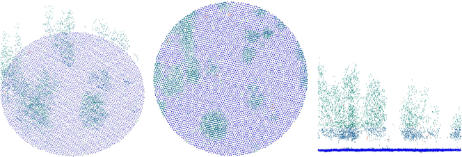
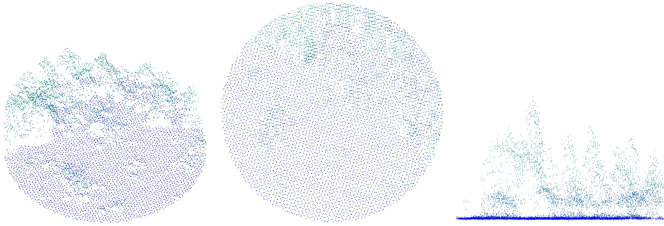
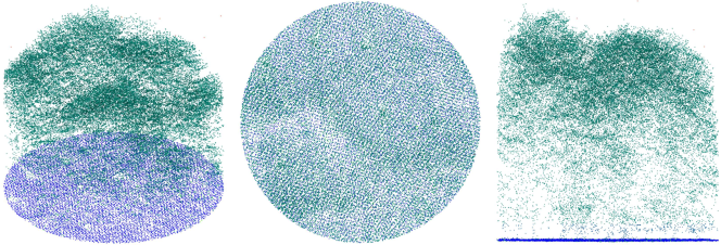
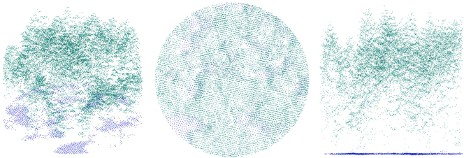
This study brings forward deep learning systems to improve forest biomass and wood volume quantification based on airborne LiDAR data with high spatial resolution per sample (). Specifically, we propose to apply deep neural networks directly to the point clouds (see Fig. 1) instead of relying on models being based on simple statistical features (we presented the initial idea as a poster in Oehmcke et al. (2022)). We hypothesize that maintaining the full dimensions of the point cloud, and hereby preventing the information loss associated with reducing dimensionality into a few statistical features strengthens predictions. The experimental evaluation shows that predictions using deep learning are considerably more accurate than currently employed methods. Further, in contrast the currently employed methods, our approach requires neither a digital terrain model (DTM) nor a CHM. This may pave the way for a paradigm shift for LiDAR-based analyses of biomass dynamics.
2 Methods
In the following, we first introduce the data used in this study in Section 2.1, which combines field-based biomass and wood volume measurements with ALS point clouds. Afterwards, in Section 2.2 the assessed deep learning architectures are presented along with their required adjustments for point cloud regression. The established baseline methods, which rely on statics derived from the point clouds are discussed in Section 2.3. Finally, we give details on why and how to correct the bias for least-square regression tasks in Section 2.4.
2.1 Forest Data
This section gives details on the two used data sources and their processing. First, the inventory data of AGB and wood volume are described, as well as how they were collected. Then, we report on the LiDAR data linked to these measurements.
2.1.1 Forest Inventory
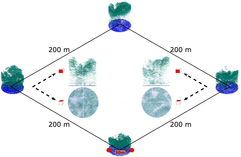
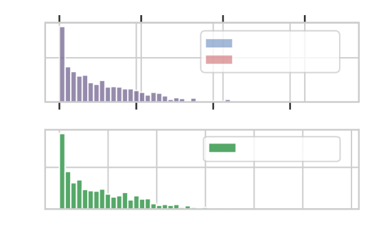
The volume (in m3 ha-1) and biomass (Mg (metric ton) ha-1) estimates used to train and evaluate the deep learning models stem from the Danish National Forest Inventory (NFI), see Fig. 3(a) for their distribution. The Danish NFI is based on a grid with cells of size covering the entire land surface of the country (Nord-Larsen and Johannsen, 2016). A plot is composed of four circular subplots with a radius of . Each subplot is located in the corners of a square, which is randomly placed within each grid cell (Fig. 2). The full set of plots is geographically partitioned into five spatially balanced interpenetrating panels (Kish, 1998; McDonald, 2003; Olsen et al., 1999; Zhang et al., 2003). Each year within a 5-year cycle, a different panel is measured, representing one fifth of the total set but representative of the entire country. These labeled data used in our study range from 2013 to 2017.
frequency
frequency
| volume m3 ha-1 |
| biomass Mg ha-1 |
| carbon Mg ha-1 |
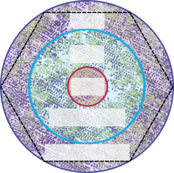
In the Danish NFI, each subplot is composed of three concentric circles with radii of , , and , respectively. Following standard procedures, a single caliper measurement of diameter is made at breast height () (i.e., from the ground) for all trees in the circle. Trees with larger than are measured in the circle, and only trees with larger than were recorded in the circle (see Fig. 3(b)). For a random sub-sample, further measurements of the total height (h), crown height (), age, and diameter at stump height () of two to six trees within each subplot are also obtained.
Based on the sub-sample measured for both and , models were developed for each species and growth region. These models are based on the observed mean height and mean diameter within each subplot for creating localized regressions using the approach suggested by Sloboda et al. (1993). For subplots where no height measurements were available, generalized regressions were developed based on a modified Näslund-equation (Näslund, 1936; Johannsen, 1999). Subsequently, individual tree volume and biomass were estimated using species-specific models (Nord-Larsen et al., 2017a). Since trees were measured in different concentric circles depending on their diameter, the volume of growing stock and biomass in each subplot were calculated by scaling the estimated AGB and wood volume of each tree according to the circular area in which the tree was measured. Carbon stocks can be considered as a linear function of the forest biomass, thus, in this study was not used as a separate regression target.

2.1.2 Point Cloud Data
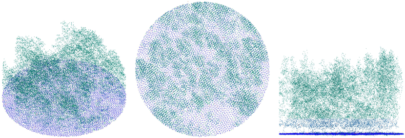
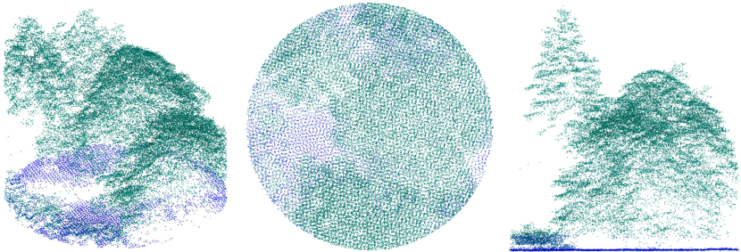
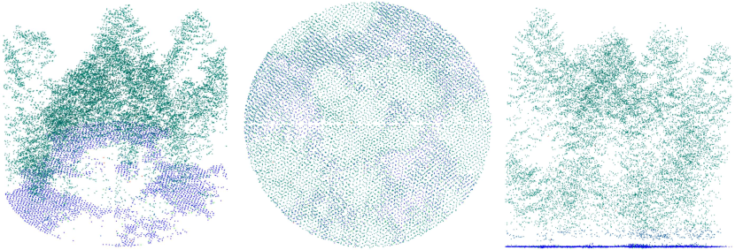
Airborne LiDAR point cloud data covering the whole of Denmark from 2014 to 2018 are publicly available from the Danish Agency for Data Supply and Efficiency (https://dataforsyningen.dk). Specifically, a sampling campaign in 2014 and 2015 covered the entire country, while a fifth of the country was again scanned in 2018 (in eastern Jutland and Funen). The average resolution of the point clouds was reported to be points per m2 with a vertical and horizontal point accuracy (given as root mean squared error (RMSE)) of and , respectively. We extracted the point clouds corresponding to the subplots studied in the NFI (see Fig. 4). The average number of points per subplot equaled with a standard deviation of points.
2.1.3 Preprocessing
Several preprocessing steps were conducted for both the deep neural networks (operating on the point clouds) as well as for the baseline models that operate on simple statistical features.
For the plot-specific point clouds, the NFI identified four types of errors. In the first type, trees visible in the point cloud do not belong to the field-based measurements but reach into the plot from the outside, while in the second type non-forest objects, such as land-lines or buildings, are part of the point cloud. We chosen not to exclude these data since a method that directly works with the point cloud should detect irrelevant parts by itself, meaning that some previously excluded data should now be usable. The third error type occurs when the plot had been harvested in-between field measurements and airborne point cloud acquisition. Finally, the fourth error type consisted of unreasonable values. Since the third and fourth error flags are intractable, the samples were excluded from the model training. In addition, all samples with no points above were removed, as this was the minimal height considered for the biomass measurements111Keeping these samples would simply reduce the errors, because they could be handled by a simple rule that predicts zero if the maximum height is below ..
The remaining dataset consists of individual point clouds, each being labelled with a corresponding biomass and wood volume measurement as described in Sec. 2.1. The biomass and wood volume were measured at different times than the collection of point clouds. To ensure that both data sources matched, we only considered point clouds observed within one year of the biomass measurement for our validation and test set. For training, we took larger temporal gaps (up to nine years) into account and added the time interval in years as a feature to the point clouds. Since some sites were measured multiple times, we kept measurements from the same site together in either training, validation, or test datasets (i.e., no site/plot considered during training or for validation occurred in the test set).
Finally, to train, validate and test all the models, we split the data as follows: the training set contains samples with a time interval of more than one year and samples with an even longer time interval (i.e., training samples in total). The validation set consists of and the test sets of samples with a maximum distance of one year between paired point cloud and biomass measurements.
2.2 Deep Regression for Point Clouds
From a mathematical perspective, a single point cloud can be represented via a set , where is the number and the dimensionality of the points (typically, ). Besides these coordinates, additional information is often provided for each point, such as color or intensity. These features paired with the points define the set
| (1) |
with containing the additional features. Such a point cloud is given for each instance (e.g., one subplot corresponds to one point cloud, see Fig. 4). The point cloud sets typically have different cardinalities and are unordered. Accordingly, the output of a model should not depend on the order of the provided points, a property referred to as permutation invariance. Furthermore, the spatial structure of such point clouds can be highly irregular and the density of points is typically very sparse (such characteristics usually vary among different regions as well).
Compared to deep convolutional neural networks (CNNs) for standard 2D and 3D images, the research field of deep learning for point cloud data has yet to mature. There are several approaches for adapting neural networks for point cloud processing, differing among others in how they deal with the key questions of how to extend the concept of spatial convolutions to sparse point clouds. Most deep learning systems for point clouds are developed for segmentation and other classification tasks (Hackel et al., 2017; Chang et al., 2015; Wu et al., 2015). In this study, we focused on regression tasks. We adapted and compared three widely-used and conceptually different point cloud classification approaches for regression: the classic PointNet (Qi et al., 2017), the kernel point convolution (KPConv) (Thomas et al., 2019), and a Minkowski CNN (Choy et al., 2019).
We extended the open-source library Torch-Points3D (Chaton et al., 2020) to support regression and will contribute our networks and anonymized dataset to the library upon acceptance of this manuscript.
2.2.1 PointNet
The seminal PointNet is one of the first deep learning architectures developed for point clouds (Qi et al., 2017). PointNet-type networks apply the same weight matrices to each input point. That is, the resulting feature maps are defined by a shared (dense) neural network. The original architecture is based on the use of multiple such neural network blocks. In between these blocks, input/feature transformations are used to align the data via learnable transformation matrices. At the end, to facilitate a variable number of points and to achieve permutation invariance, a symmetric set function is applied, which can be simply a global max-pooling operation. Two PointNet variants have been proposed in the seminal work to address classification and segmentation scenarios, respectively.
To adapt the architecture for regression, we adopted the classification PointNet architecture up to the global feature aggregation. We then replaced the subsequent two hidden fully-connected layers (output dimensionalities: 512-256) with three fully-connected layers (output dimensionalities: 512-256-128) and considered a final linear output layer.
2.2.2 KPConv
The kernel point convolution (Thomas et al., 2019) extends standard discrete convolution to the domain of point clouds. Kernel point convolutions consider, for a given input point , a local neighborhood along with points called kernel points that are used to define a convolution operator. More precisely, is convolved by a kernel at a point is defined via
| (2) |
Here , where is a hyper-parameter defining the domain of the kernel . The kernel is based on a set of kernel points, where each kernel point has an associated weight matrix , which maps a feature vector to a new feature vector (for the first such convolution layer, we have ). One option for the kernel is
| (3) |
where and is a user-defined model parameter (Thomas et al., 2019). Thus, the kernel yields a weighted sum of weight matrices and each kernel is parameterized by its own kernel points and the corresponding weight matrices. The weight matrices are learnt similarly to the coefficients of convolution operators in standard CNNs. The kernel points can either also be learnt (“deformable”) or can be fixed (“rigid”) systematically around the center of (Thomas et al., 2019). Pooling operations are realized via creating a 3D grid in which all points in a cell are aggregated (see Sec. 2.2.3).
We adapt the KPConv architecture proposed for classification (KP-CNN) to utilize it for regression. KP-CNN follows the structure of ResNet, thus modifying it for regression was straightforward and was achieved by changing the output layer to have the identity as activation function. We resorted to fixed kernel points since deformable ones consistently performed worse on our dataset.
2.2.3 Minkowski Convolutional Neural Network
A straightforward approach to process point clouds is to voxelize the points to a 3D image (with channels) and to apply a standard 3D convolutional neural network (CNN) to the resulting image. This requires binning, but while a coarse binning may discard important information, a fine-grained binning can render the computations intractable. However, the points are typically very sparse in 3D space. This lends to keeping a sparse representation and applying spatially sparse 3D convolutions, which basically operate only in areas where points exist (Graham, 2015; Graham et al., 2018). A state-of-the-art implementation of sparse convolutions for point clouds is given by the Minkowski Engine, an auto-differentiation library, which allows to efficiently implement standard architectures, such as ResNet with 3D convolutions (Choy et al., 2019).
Both the Minkowski and KPConv architectures progressively downsample the point cloud based on a 3D grid via pooling operations. The initial grid size is only bound to the horizontal and vertical accuracy of the point data, meaning that a too small grid size cannot be processed efficiently. Therefore, it is crucial to set the initial grid size according to the data and task. The subsequent pooling steps are then based on this initial size and work similarly to standard 2D pooling operations. Once a grid is created, a voxel-based approach, such as Minkowski CNNs, aggregates all voxels within a grid cell to a new voxel. In contrast, KPConv takes the mean of the position of all points within a cell to form a new point. By doubling the size of the grid cells in each subsampling/pooling layer, the number of points/voxels is gradually reduced, corresponding to an increase in the size of the receptive field The features associated with each new point can be obtained, for example, via max-pooling (applied to the feature vectors of the pooled points) or by applying the chosen convolution operator.
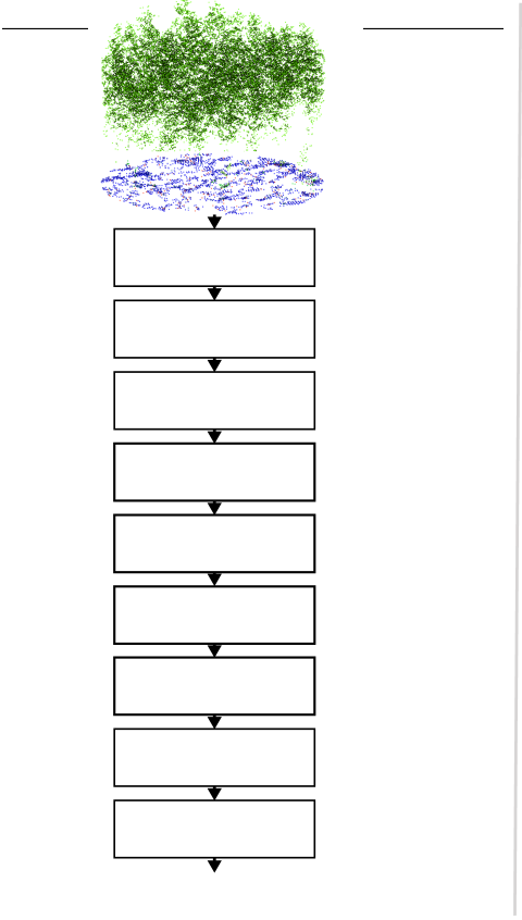
Using the Minkowski Engine library, we built two 3D versions of SENet (SENet14 and SENet50) for regression (Hu et al., 2018), see Fig. 5. To that end, we replaced 2D convolutions with their 3D equivalent. The stride of the initial convolution of SENet was changed from to in order to avoid early loss of information. We also replaced Rectified Linear Unit (ReLU) activation functions with Exponential Linear Units (ELU) (Clevert et al., 2016). Finally, the output layer was changed to fit the number of target variables and does not apply a non-linear activation. The two network versions differ in the number of trainable parameters as shown in Tab. 1 and are referred to as MSENet14 and MSENet50, respectively.
| single point |
| grid size |
| SEBlock |
| Conv3D |
| max pool |
| glob. avg. pool |
| FC |
| SEBlock |
| SEBlock |
| SEBlock |
| GridSample |
| stride |
| stride |
| stride |
| stride |
| stride |
| predicted AGB & wood volume |

| Conv3D |
| glob. avg. pool |
| Conv3D |
| Conv3D |
| FC |
| FC |
| ELU |
| sigmoid |
| scale |
| add |
| residual |
squeeze & excite
| stride |
2.2.4 Experimental Setup for Forest Attribute Regression
Three different neural network architectures were applied: the proposed regression versions of PointNet, KPConv, and two 3D version of SENet (MSENet14 and MSENet50) built with the Minkowski Engine. All code was written in Python and PyTorch (Paszke et al., 2019) and trained on A100 GPUs. The positions of the input points were given in the projected coordinate system EPSG:25832. We centered the -, -, and -coordinates for each subplot individually to get a local reference frame. Scaling was applied by dividing by , , , respectively, so that the coordinates lie within for the - and -coordinates. We do not need to calibrate our model using a DTM, as is required by state-of-the-art methods based on point cloud statistics.
We tuned the initial grid size of KPConv and the MSENet models by gradually decreasing it (i.e., increasing the spatial resolution) until no improvement could be seen on the validation set. Both architectures worked best with the initial grid size set to . The number of trainable model parameters and runtimes are given in Tab. 1.
| Model | number of parameters | test time | train time |
|---|---|---|---|
| PointNet | 7s | 7h | |
| KPConv | 55s | 42h | |
| MSENet14 | 4s | 4h | |
| MSENet50 | 5s | 9h |
To increase diversity in the training set, several augmentations were considered. First, a random rotation around the z-axis was applied. We did not consider rotating the x- and y-axis since a tilt would result in unrealistic samples (e.g., change of growth direction). Thereafter, random dropout of points with a dropout rate of 20% in 50% of all samples was applied, which increases variety and simulates changes in point density. Finally, each dimension of the point position was shifted by adding a small random value drawn from a zero-mean truncated Gaussian distribution with variance and support .
One goal was to create precise wood volume and above-ground biomass maps over large areas. Therefore, instead of using the entire circle in which the measurements were taken, we resorted to a hexagonal shape in the x- and y-coordinate, see Fig. 3(b). This approach facilitates an easy tiling of large areas without gaps and overlaps. The hexagonal shape covers almost all of the points, in particular those in the inner circles (in control experiments, we verified that considering the whole subplot does not lead to a significant performance increase).
We employed the AdamW (Loshchilov and Hutter, 2019) optimizer with weight decay set to . The initial learning rate was , which was adapted according to the cosine annealing schedule with warm restarts () (Loshchilov and Hutter, 2017) for epochs. The batch size was and the smooth L1 function Girshick (2015) was used as training loss. These hyper-parameter configurations were chosen based on the highest score on the validation set. The input channel was filled with ones to encode the presence of a point.
2.3 Baseline Methods
The baseline models considered in this study for estimating above-ground biomass, rely on precomputed features from the normalized height distribution in accordance with Nord-Larsen et al. (2017b): mean height, height standard deviation, coefficient of variation, skewness, kurtosis, percentiles of the height distribution (5, 10, 25, 50, 75, 90, 95, 99), and the interception ratio (IR), which is the fraction of points above one meter compared to all first returns. For each point cloud sample, these features except the IR were computed twice, once for all points and once only for the points above ground. To determine the height of a point relative to the ground, we calibrated it semi-automatically, using two DTMs with different spatial resolutions ( and ), and the first return of each light pulse from the airborne LiDAR, following the study of Magnussen et al. (2018). In preliminary analysis, it was observed that this approach led to better results than using all the recorded returns from each LiDAR-derived light pulse. In contrast, the deep learning methods simply use all the information included in the point clouds without the need to filter out the point cloud datasets according to the number of returns. In total, statistical features were extracted for each point cloud sample.
2.3.1 Linear and Power Regression
The first two baseline methods were linear regression and power regression models. For the linear regression models, all the features were used as explanatory variables. The multivariate power regression can be regarded as the state-of-the art for predicting AGB, above-ground carbon stocks, and tree volume from the point cloud features (Magnussen et al., 2018). Following Magnussen et al. (2018), we fitted models of the form
| (4) |
for each quantity of interest. Here, is the mean height of the points one meter above ground, is the 95 percentile of the height distribution of point one meter above ground, and IR is the inception ratio. For each model, the parameters were set to the optimal least-squares estimates.
2.3.2 Random Forest
We trained random forest (RF) models with trees (Breiman, 2001) and resorted to the popular Scikit-Learn implementation (Pedregosa et al., 2011). The out-of-bag (OOB) error was used to tune the RF hyper-parameters. We considered for the ratio of features to consider at every split, for the ratio of samples to consider for each tree, for the maximum tree depth, and for the minimum number of samples required at each leaf node. The best model used 90% of the features at every split, 20% of the training data for each tree, had a maximum depth of , and required a minimum number of samples at each leaf node.
2.4 Bias Correction
Least-squares regression with deep learning models typically lead to biased models in the sense that the sum of residuals on the training data set is not zero (Igel and Oehmcke, 2022). Consider a regression model of the form
| (5) |
with parameters . Here for some positive integer , , , . This model can be a deep neural network, where all layers but the final layer are represented by the function and the parameters comprise all weights except those in the final layer. Training a deep neural network for regression using iterative optimization with mini-batches and stopping after a fixed training time or based on performance on a hold-out data set cannot be expected to chose the parameter in a way that the residuals on the training data sum to zero. That is, on the training data we have . This can introduce a systematic error that accumulates if we are interested in the total aggregated performance over many data points. We therefore used the method proposed by Igel and Oehmcke (2022) to correct this bias by replacing by
| (6) |
3 Results
We conducted a detailed comparison of all methods for predicting AGB (and thereby above-ground carbon stocks) and wood volume. We used the root-mean-square-error (RMSE), the coefficient of determination , and the mean absolute percentage error (MAPE) as evaluation metrics, in accordance with the related literature. The prediction bias parameter was calibrated on the training and validation set for all non-linear methods (all except linear regression) as described in Section 2.4 (Igel and Oehmcke, 2022).
An overview of the results is given in Tab. 2 showing the , RMSE, and MAPE for the different algorithms on the test set, which was not used for model development. Overall, the MSENet14 model achieved the best results with an of for biomass (and carbon stocks) and an of for wood volume. The corresponding RMSEs were Mg ha-1 and m3 ha-1, respectively.
| RMSE | MAPE | ||||||
|---|---|---|---|---|---|---|---|
| target | model | med. | max | med. | min | med. | min |
| AGB | linear | ||||||
| power | |||||||
| RF | |||||||
| PointNet | |||||||
| KPConv | |||||||
| MSENet14 | |||||||
| MSENet50 | |||||||
| volume | linear | ||||||
| power | |||||||
| RF | |||||||
| PointNet | |||||||
| KPConv | |||||||
| MSENet14 | |||||||
| MSENet50 | |||||||
The RF performed the worst. The better performance of the linear regression with an of for biomass and for wood volume, indicates that the calculated features are to a certain extend linearly correlated with the target variables. The power regression model based on Magnussen et al. (2018) reached values of and for biomass and tree volume, respectively, that is, the deep learning approach clearly improved over the state-of-the-art methods. All more recent point cloud based methods outperformed the models based on the precomputed features, justifying that the networks indeed utilized additional information from the point clouds. The MAPE, which was not an optimization criterion, showed the largest differences between the methods, which are mainly attributed to errors related to small target values.
The national forest inventory data offers information about the fraction of conifer and broadleaf for each site, which we used to analyze the performance at different fractions in Fig. 6. Interestingly, KPConv performed better than the Minkowski models for conifer fraction interval and nearly equally good at 100. Again, the high MAPE for the baseline methods that rely on the precomputed features and PointNet was noticeable, in particular when mono cultures were analyzed. In general, mono cultures turned out to be more difficult than mixed forests w.r.t. MAPE but not w.r.t. RMSE and (e.g., forests with conifer trees only exhibited the lowest RMSE and ).

| linear |
| power |
| RF |
| PointNet |
| KPConv |
| MSENet14 |
| MSENet50 |
| 0.0 |
| 0.2 |
| 0.6 |
| 0.4 |
| 0.8 |
| 0 |
| (0, 33] |
| (33, 66] |
| (66, 100) |
| 100 |
conifer fraction
| 0 |
| 20 |
| 40 |
| 60 |
| RMSE |
| 0 |
| 2000 |
| 4000 |
| MAPE |
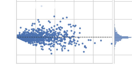
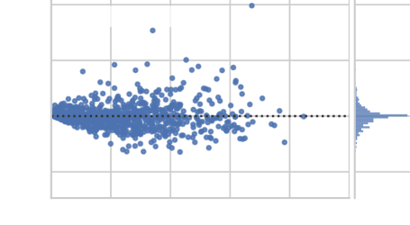
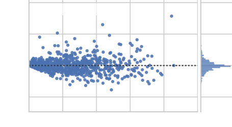
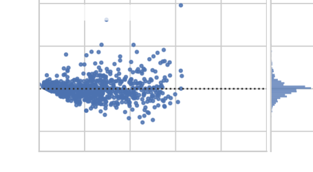
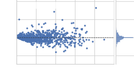
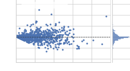
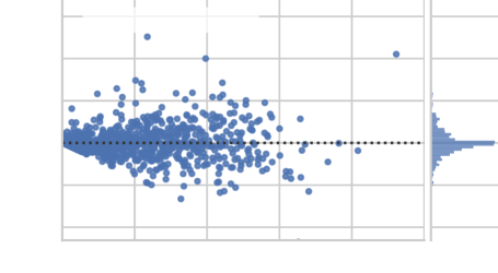
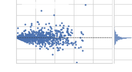
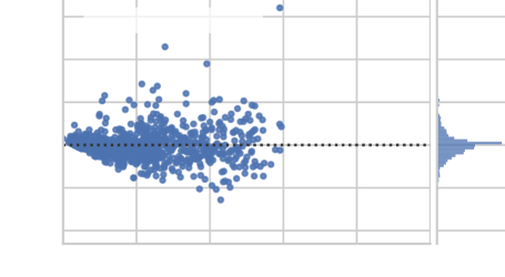
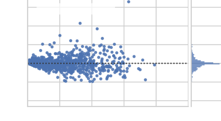
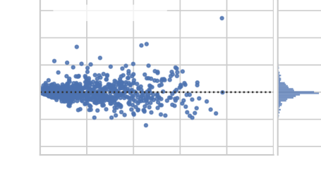
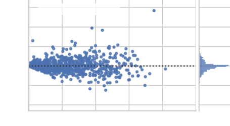
The spread of errors increased with magnitude of the target variables as seen in Fig. 7 for the power, KPConv, and MSENet14 model. While low values were more often overestimated, high values tended to be underestimated. Comparing the distribution of errors as well as the mean error of the assessed models, one can see that the KPConv and Minkowski models had a generally lower spread of errors than the power model. See Fig. 11 and 12 in the appendix for the remaining plots.
| mean error: 2.03 Mg ha-1 |
| 0 |
| 100 |
| 200 |
| 300 |
| 400 |
| 500 |
| predicted AGB |
| -200 |
| 0 |
| 200 |
| 400 |
residuals
| mean error: 0.46 Mg ha-1 |
| 0 |
| 100 |
| 200 |
| 300 |
| 400 |
| 500 |
| predicted AGB |
| -200 |
| 0 |
| 200 |
| 400 |
residuals
| mean error: 0.36 Mg ha-1 |
| 0 |
| 100 |
| 200 |
| 300 |
| 400 |
| 500 |
| predicted AGB |
| -200 |
| 0 |
| 200 |
| 400 |
residuals
It has been found that the errors of ALS-based carbon stock estimates decrease when increasing the size of the observed area (e.g., aggregating over a larger area decreases the error (Asner et al., 2010; Mascaro et al., 2011; Dalponte and Coomes, 2016; Ferraz et al., 2016)). To demonstrate this, we calculated the RMSE for each model over the same randomly chosen combination of subplots (Fig. 8). We repeated that process 10 times with different random combinations for each model repetition. The predictions for the combined plots were added and compared to the aggregated measurements. We consider the carbon stock RMSE in Mg C ha-1 to allow for easier comparison with published results. The RMSE reduces quickly for all models and the ranking of models remains the same.

| 0 |
| 10 |
| 20 |
| 30 |
| 40 |
| 50 |
| 60 |
| 70 |
| 80 |
| 90 |
| number of samples |
| 5 |
| 10 |
| 15 |
| 20 |
| 25 |
RMSE
| linear |
| power |
| RF |
| PointNet |
| KPConv |
| MSENet14 |
| MSENet50 |
| 86 |
| 87 |
| 88 |
| 89 |
| 90 |
| number of samples |
| 2.0 |
| 2.5 |
| 3.0 |
RMSE
| 13 |
| 14 |
| 15 |
| 16 |
| number of samples |
| 5 |
| 6 |
| 7 |
RMSE
| 6.02 |
| 6.09 |
| 6.16 |
| 6.23 |
| 6.30 |
| 0.91 |
| 0.98 |
| 1.05 |
| 1.12 |
| area in ha |
| area in ha |
| 1 |
| 0.7 |
| 1.4 |
| 2.1 |
| 2.8 |
| 3.5 |
| 4.2 |
| 4.9 |
| 5.6 |
| 6.3 |
| 0.07 |
| area in ha |
4 Discussion
The results give clear evidence that the deep learning approaches KPConv and MSENet are preferable to the methods working on point cloud statistics. As the time to apply and train MSENet is drastically shorter (see Tab. 1) and the results were marginally better, we regard MSENet as the method of choice. We assume that the subpar performance of PointNet is due to the missing local context processing in the algorithm, which seems to be required for forest scenes.
4.1 Quantitative comparison to other studies
Caution is warranted when comparing our prediction accuracy with that of other studies. Reported errors of ALS-based prediction models for AGB range from to Mg ha-1 in the tropics (Asner et al., 2011), and this error is comparable to estimates reported in other regions (Lefsky et al., 2002) as well as previous studies with the Danish NFI (Nord-Larsen and Schumacher, 2012). Reassuringly, we achieve error rates at the lower end of this spectrum. It is important to emphasize, however, that it is not uncommon that the indicators documented in these studies measure the error on a training data set as a goodness of fit index (Lefsky et al., 1999, e.g., in the study by the for AGB drops from 80 % down to 33 % when the model is applied to a different data set). Similarly but not as severe, earlier studies of the Danish NFI with fewer data also reported a % increase in RMSE when using hold-out sets (Nord-Larsen and Schumacher, 2012). Conversely, the training errors of our models are similar to the test set results in Tab. 2 (see Tab. 3 in the supplementary material), indicating that the models are not overfitted.
The error of the overall carbon stock prediction has been shown to decrease with increasing area, which is explained by error cancellation (Asner et al., 2010; Mascaro et al., 2011; Dalponte and Coomes, 2016; Ferraz et al., 2016; Magnussen et al., 2018). This is an important property when it comes to country-wide quantification of carbon. For example, in the study by Mascaro et al. (2011), the RMSE of the estimated carbon stocks decreased from to and then to Mg C ha-1 when the observed area was increased from to and then to . Our study areas are of size . The residuals in Fig. 7 indeed suggest that our errors average out if several subplots are combined. This is confirmed by the results shown in Fig. 8. For aggregated areas of approximately (with 14 samples it is ) and (with 89 samples it is ), the RMSE for the MSENet14 model was (SE ) and (SE ), respectively. Even though the errors cancel out, a good high-resolution performance seems to translate to a better aggregated performance.
4.2 Applicability and map generation
The results are evaluated on an previously unseen and non-overlapping test set, meaning that the model should exhibit a similar performance on other arbitrarily chosen forest subplots from the study area (e.g., Denmark). For new study areas that are dissimilar to ours (e.g., different climate zone, tree species, or topographical features), reevaluation and potential fine-tuning of the models would be needed. However, since little preprocessing is required, this verification and adjustment step is comparatively minor.
Our method allows for dense, non-interpolated biomass mappings with unprecedented accuracy at large scale at a resolution below . An exemplary biomass map is demonstrated in Fig. 9. The figure shows the results of the MSENet50 model applied to a randomly selected area in Denmark without any additional preprocessing. The results are convincing, as areas with no points above ground are predicted to have no biomass, and areas with many trees have high biomass. Thus, our method enables highly accurate analyses of the AGB development in Denmark by comparing AGB maps from different years.

| 0 |
| 100 |
| m |
| 0 |
| 30 |
| m |
| 0 |
| 15 |
| 30 |
| 0-31 |
| 0 |
| 31-74 |
| 74-112 |
| 112-146 |
| 146-172 |
| 172-197 |
| 197-224 |
| 224-257 |
| 257-296 |
| 296-340 |
| 340-432 |
| 60 |
| 200 |
| m |
| N |
5 Conclusions
Precise quantification of the spatial distribution of forest biomass and carbon content is a valuable tool to understand the processes driving af-, re-, and deforestation, and the variations in carbon cycle from the ecosystem to the regional and global scale (Zolkos et al., 2013).
This study brings forward deep learning systems for predicting above-ground biomass, wood volume, and carbon stocks in forests efficiently and directly from airborne LiDAR point clouds. Three conceptually different neural network architectures for classification (i.e., PointNet, KPConv, and Minkowski CNNs) were modified to perform regression, and were evaluated using a unique data set combining field measurements and LiDAR data.
Our adaptation of Minkowski CNNs outperformed the other deep learning approaches as well as the baseline methods. Specifically, the coefficient of determination for above-ground biomass and stored carbon exceeded at on a test set, which was not considered in the modelling process. The main advantage of the method proposed is the efficient implementation of 3D convolutions for sparse data, as it relies on the same operations that CNNs use for standard image processing.
The assessed deep learning models achieved high accuracies, leading to a considerably better performance in predicting AGB of forest areas, compared to the state-of-the-art approach operating on basic statistics of the point clouds. Our approach simplifies the production of AGB and carbon content maps at high resolution. It does neither require digital elevation models (e.g., DTMs or canopy height models) nor forest canopies with structural heterogeneity.
These encouraging results may be the first step towards a paradigm shift in utilizing LiDAR data for accurate quantification and analysis of forest carbon dynamics, which is a key component for achieving the United Nations Strategic Plan for Forests under the Paris agreement and the Sustainable Development Goals (SDGs) (United Nations Department of Economic and Social Affairs, 2021; United Nations Department of Economic and Social Affairs, 2017) in accordance with the IPCC 2018 (Masson-Delmotte et al., 2019)).
Acknowledgement
This work was supported by the research grant DeReEco (34306) from Villum Foundations, the Independent Research Fund Denmark through the grant Monitoring Changes in Big Satellite Data via Massively-Parallel Artificial Intelligence (9131-00110B), a Villum Experiment grant by the Velux Foundations (MapCland project, project number: 00028314), the DeepCrop project (UCPH Strategic plan 2023 Data+ Pool), and the Pioneer Centre for AI, DNRF grant number P1.
References
- Asner and Mascaro [2014] Gregory P Asner and Joseph Mascaro. Mapping tropical forest carbon: Calibrating plot estimates to a simple lidar metric. Remote Sensing of Environment, 140:614–624, 2014.
- Asner et al. [2010] Gregory P Asner, George VN Powell, Joseph Mascaro, David E Knapp, John K Clark, James Jacobson, Ty Kennedy-Bowdoin, Aravindh Balaji, Guayana Paez-Acosta, Eloy Victoria, et al. High-resolution forest carbon stocks and emissions in the Amazon. Proceedings of the National Academy of Sciences, 107(38):16738–16742, 2010.
- Asner et al. [2011] Gregory P. Asner, R. Flint Hughes, Joseph Mascaro, Amanda L. Uowolo, David E. Knapp, James Jacobson, Ty Kennedy-Bowdoin, and John K. Clark. High-resolution carbon mapping on the million-hectare island of Hawaii. Frontiers in Ecology and the Environment, 9(8):434–439, 2011.
- Bouvier et al. [2015] Marc Bouvier, Sylvie Durrieu, Richard A Fournier, and Jean-Pierre Renaud. Generalizing predictive models of forest inventory attributes using an area-based approach with airborne lidar data. Remote Sensing of Environment, 156:322–334, 2015.
- Breiman [2001] Leo Breiman. Random forests. Machine Learning, 45(1):5–32, 2001.
- CARTO [2023] CARTO. map style. https://carto.com/, 2023.
- Chang et al. [2015] Angel X. Chang, Thomas A. Funkhouser, Leonidas J. Guibas, Pat Hanrahan, Qi-Xing Huang, Zimo Li, Silvio Savarese, Manolis Savva, Shuran Song, Hao Su, Jianxiong Xiao, Li Yi, and Fisher Yu. Shapenet: An information-rich 3D model repository. CoRR, abs/1512.03012, 2015.
- Chaton et al. [2020] Thomas Chaton, Chaulet Nicolas, Sofiane Horache, and Loic Landrieu. Torch-Points3D: A modular multi-task frameworkfor reproducible deep learning on 3D point clouds. In 3D Vision (3DV), pages 1–10. IEEE, 2020.
- Choy et al. [2019] Christopher Choy, JunYoung Gwak, and Silvio Savarese. 4D spatio-temporal convnets: Minkowski convolutional neural networks. In IEEE / CVF Computer Vision and Pattern Recognition Conference (CVPR), pages 3075–3084, 2019.
- Clevert et al. [2016] Djork-Arné Clevert, Thomas Unterthiner, and Sepp Hochreiter. Fast and accurate deep network learning by exponential linear units (ELUs). In International Conference on Learning Representation (ICLR), 2016.
- Cook-Patton et al. [2020] Susan C Cook-Patton, Sara M Leavitt, David Gibbs, Nancy L Harris, Kristine Lister, Kristina J Anderson-Teixeira, Russell D Briggs, Robin L Chazdon, Thomas W Crowther, Peter W Ellis, et al. Mapping carbon accumulation potential from global natural forest regrowth. Nature, 585(7826):545–550, 2020.
- Coyle et al. [2019] D. Barry Coyle, Paul R. Stysley, Furqan L. Chirag, Erich Frese, and Demetrios Poulios. The global ecosystem dynamics investigation (GEDI) LiDAR laser transmitter. In Infrared Remote Sensing and Instrumentation XXVII, volume 11128, pages 112–125. Int. Society for Optics and Photonics, 2019.
- Dalponte and Coomes [2016] Michele Dalponte and David A Coomes. Tree-centric mapping of forest carbon density from airborne laser scanning and hyperspectral data. Methods in ecology and evolution, 7(10):1236–1245, 2016.
- d’Oliveira et al. [2012] Marcus VN d’Oliveira, Stephen E Reutebuch, Robert J McGaughey, and Hans-Erik Andersen. Estimating forest biomass and identifying low-intensity logging areas using airborne scanning lidar in antimary state forest, acre state, western brazilian amazon. Remote Sensing of Environment, 124:479–491, 2012.
- Erb et al. [2018] Karl-Heinz Erb, Thomas Kastner, Christoph Plutzar, Anna Liza S Bais, Nuno Carvalhais, Tamara Fetzel, Simone Gingrich, Helmut Haberl, Christian Lauk, Maria Niedertscheider, Julia Pongratz, Martin Thurner, and Sebastiaan Luyssaert. Unexpectedly large impact of forest management and grazing on global vegetation biomass. Nature, 553(7686):73–76, 2018.
- FAO and UNEP [2020] FAO and UNEP. The state of the world’s forests 2020. forests, biodiversity and people, 2020.
- Fassnacht et al. [2014] FE Fassnacht, F Hartig, H Latifi, C Berger, J Hernández, P Corvalán, and B Koch. Importance of sample size, data type and prediction method for remote sensing-based estimations of aboveground forest biomass. Remote Sensing of Environment, 154:102–114, 2014.
- Ferraz et al. [2016] António Ferraz, Sassan Saatchi, Clément Mallet, and Victoria Meyer. Lidar detection of individual tree size in tropical forests. Remote Sensing of Environment, 183:318–333, 2016.
- Firintepe et al. [2021] Ahmet Firintepe, Carolin Vey, Stylianos Asteriadis, Alain Pagani, and Didier Stricker. From IR images to point clouds to pose: Point cloud-based AR glasses pose estimation. Journal of Imaging, 7(5), 2021. ISSN 2313-433X.
- Ge et al. [2018] Liuhao Ge, Zhou Ren, and Junsong Yuan. Point-to-point regression PointNet for 3D hand pose estimation. In European Conference on Computer Vision (ECCV), pages 475–491, 2018.
- Girshick [2015] Ross Girshick. Fast R-CNN. In International Conference on Computer Vision (ICCV), pages 1440–1448, 2015.
- Goetz and Dubayah [2011] Scott Goetz and Ralph Dubayah. Advances in remote sensing technology and implications for measuring and monitoring forest carbon stocks and change. Carbon Management, 2(3):231–244, 2011.
- Goodwin et al. [2006] Nicholas R Goodwin, Nicholas C Coops, and Darius S Culvenor. Assessment of forest structure with airborne lidar and the effects of platform altitude. Remote Sensing of Environment, 103(2):140–152, 2006.
- Graham [2015] Ben Graham. Sparse 3D convolutional neural networks. In BMVC, pages 150.1–150.9, 2015.
- Graham et al. [2018] Benjamin Graham, Martin Engelcke, and Laurens Van Der Maaten. 3D semantic segmentation with submanifold sparse convolutional networks. In IEEE / CVF Computer Vision and Pattern Recognition Conference (CVPR), pages 9224–9232, 2018.
- Griscom et al. [2017] Bronson W. Griscom, Justin Adams, Peter W. Ellis, Richard A. Houghton, Guy Lomax, Daniela A. Miteva, William H. Schlesinger, David Shoch, Juha V. Siikamäki, Pete Smith, Peter Woodbury, Chris Zganjar, Allen Blackman, João Campari, Richard T. Conant, Christopher Delgado, Patricia Elias, Trisha Gopalakrishna, Marisa R. Hamsik, Mario Herrero, Joseph Kiesecker, Emily Landis, Lars Laestadius, Sara M. Leavitt, Susan Minnemeyer, Stephen Polasky, Peter Potapov, Francis E. Putz, Jonathan Sanderman, Marcel Silvius, Eva Wollenberg, and Joseph Fargione. Natural climate solutions. Proceedings of the National Academy of Sciences, 114(44):11645–11650, 2017.
- Guo et al. [2020] Yulan Guo, Hanyun Wang, Qingyong Hu, Hao Liu, Li Liu, and Mohammed Bennamoun. Deep learning for 3d point clouds: A survey. transactions on pattern analysis and machine intelligence (PAMI), 43(12):4338–4364, 2020. doi: 10.1109/TPAMI.2020.3005434.
- Hackel et al. [2017] Timo Hackel, N. Savinov, L. Ladicky, Jan D. Wegner, K. Schindler, and M. Pollefeys. SEMANTIC3D.NET: A new large-scale point cloud classification benchmark. In ISPRS Annals of the Photogrammetry, Remote Sensing and Spatial Information Sciences, volume IV-1-W1, pages 91–98, 2017.
- Hancock et al. [2019] Steven Hancock, John Armston, Michelle Hofton, Xiaoli Sun, Hao Tang, Laura I Duncanson, James R Kellner, and Ralph Dubayah. The gedi simulator: A large-footprint waveform lidar simulator for calibration and validation of spaceborne missions. Earth and Space Science, 6(2):294–310, 2019.
- Harris et al. [2012] Nancy L Harris, Sandra Brown, Stephen C Hagen, Sassan S Saatchi, Silvia Petrova, William Salas, Matthew C Hansen, Peter V Potapov, and Alexander Lotsch. Baseline map of carbon emissions from deforestation in tropical regions. Science, 336(6088):1573–1576, 2012.
- Harris et al. [2021] Nancy L Harris, David A Gibbs, Alessandro Baccini, Richard A Birdsey, Sytze De Bruin, Mary Farina, Lola Fatoyinbo, Matthew C Hansen, Martin Herold, Richard A Houghton, et al. Global maps of twenty-first century forest carbon fluxes. Nature Climate Change, 11(3):234–240, 2021.
- Hu et al. [2018] Jie Hu, Li Shen, and Gang Sun. Squeeze-and-excitation networks. In IEEE / CVF Computer Vision and Pattern Recognition Conference (CVPR), pages 7132–7141, 2018.
- Igel and Oehmcke [2022] Christian Igel and Stefan Oehmcke. Remember to correct the bias when using deep learning for regression! Künstliche Intelligenz, 2022. (in press).
- Johannsen [1999] Vivian Kvist Johannsen. A growth model for oak in Denmark. PhD thesis, Royal Veterinary and Agricultural University, Copenhagen, Denmark, 1999.
- Kish [1998] Leslie Kish. Space/time variations and rolling samples. Journal of Official Statistics, 14(1):31, 1998.
- Knapp et al. [2018] Nikolai Knapp, Rico Fischer, and Andreas Huth. Linking lidar and forest modeling to assess biomass estimation across scales and disturbance states. Remote Sensing of Environment, 205:199–209, 2018.
- Knapp et al. [2020] Nikolai Knapp, Rico Fischer, Victor Cazcarra-Bes, and Andreas Huth. Structure metrics to generalize biomass estimation from lidar across forest types from different continents. Remote Sensing of Environment, 237:111597, 2020.
- Lang et al. [2021] Nico Lang, Konrad Schindler, and Jan Dirk Wegner. High carbon stock mapping at large scale with optical satellite imagery and spaceborne LIDAR. CoRR, 2021.
- Lang et al. [2022] Nico Lang, Nikolai Kalischek, John Armston, Konrad Schindler, Ralph Dubayah, and Jan Dirk Wegner. Global canopy height regression and uncertainty estimation from GEDI lidar waveforms with deep ensembles. Remote Sensing of Environment, 268:112760, 2022.
- LeCun et al. [2015] Yann LeCun, Yoshua Bengio, and Geoffrey Hinton. Deep learning. Nature, 521(7553):436–444, 2015.
- Lefsky et al. [1999] Michael A. Lefsky, D. Harding, W. B. Cohen, G Parker, and H. H. Shugart. Surface lidar remote sensing of basal area and biomass in deciduous forests of eastern Maryland, USA. Remote Sensing of Environment, 67(1):83–98, 1999. ISSN 0034-4257.
- Lefsky et al. [2002] Michael A. Lefsky, Warren B. Cohen, David J. Harding, Geoffrey G. Parker, Steven A. Acker, and S. Thomas Gower. Lidar remote sensing of above-ground biomass in three biomes. Global Ecology and Biogeography, 11(5):393–399, 2002.
- Lewis et al. [2019] Simon L Lewis, Charlotte E Wheeler, Edward TA Mitchard, and Alexander Koch. Regenerate natural forests to store carbon. Nature, 568(7750):25–28, 2019.
- Li et al. [2020] Yingchang Li, Mingyang Li, Chao Li, and Zhenzhen Liu. Forest aboveground biomass estimation using landsat 8 and sentinel-1a data with machine learning algorithms. Scientific Reports, 10(1):1–12, 2020.
- Loshchilov and Hutter [2017] Ilya Loshchilov and Frank Hutter. SGDR: stochastic gradient descent with warm restarts. In International Conference on Learning Representation (ICLR). OpenReview.net, 2017.
- Loshchilov and Hutter [2019] Ilya Loshchilov and Frank Hutter. Decoupled weight decay regularization. In International Conference on Learning Representation (ICLR). OpenReview.net, 2019.
- Magnussen et al. [2012] Steen Magnussen, E Næsset, T Gobakken, and G Frazer. A fine-scale model for area-based predictions of tree-size-related attributes derived from lidar canopy heights. Scandinavian Journal of Forest Research, 27(3):312–322, 2012.
- Magnussen et al. [2018] Steen Magnussen, Thomas Nord-Larsen, and Torben Riis-Nielsen. Lidar supported estimators of wood volume and aboveground biomass from the Danish national forest inventory (2012–2016). Remote Sensing of Environment, 211:146–153, 2018.
- Mascaro et al. [2011] Joseph Mascaro, Matteo Detto, Gregory P. Asner, and Helene C. Muller-Landau. Evaluating uncertainty in mapping forest carbon with airborne LiDAR. Remote Sensing of Environment, 115(12):3770–3774, 2011.
- Masson-Delmotte et al. [2019] V. Masson-Delmotte, P. Zhai, H.-O. Pörtner, D. Roberts, J. Skea, P.R. Shukla, A. Pirani, W. Moufouma-Okia, C. Péan, R. Pidcock, S. Connors, J. B. R. Matthews, Y. Chen, X. Zhou, M.I. Gomis, E. Lonnoy, T. Maycock, M. Tignor, and T. Waterfield, editors. IPCC, 2018: Global Warming of 1.5°C. An IPCC Special Report on the impacts of global warming of 1.5°C above pre-industrial levels and related global greenhouse gas emission pathways, in the context of strengthening the global response to the threat of climate change, sustainable development, and efforts to eradicate poverty. Cambridge University Press, 2019.
- McDonald [2003] Trent L. McDonald. Review of environmental monitoring methods: survey designs. Environmental Monitoring and Assessment, 85(3):277–292, 2003.
- Mermoz et al. [2015] Stéphane Mermoz, Maxime Réjou-Méchain, Ludovic Villard, Thuy Le Toan, Vivien Rossi, and Sylvie Gourlet-Fleury. Decrease of l-band sar backscatter with biomass of dense forests. Remote Sensing of Environment, 159:307–317, 2015.
- Mitchard et al. [2012] Edward T. A. Mitchard, Sassan S. Saatchi, Lee J. T. White, Katharine Anne Abernethy, Kathryn Jane Jeffery, Simon L. Lewis, Murray Collins, Michael A. Lefsky, Miguel E. Leal, Iain H. Woodhouse, and Patrick Meir. Mapping tropical forest biomass with radar and spaceborne LiDAR in Lopé National Park, Gabon: overcoming problems of high biomass and persistent cloud. Biogeosciences, 9(1):179–191, 2012.
- Næsset [2009] Erik Næsset. Effects of different sensors, flying altitudes, and pulse repetition frequencies on forest canopy metrics and biophysical stand properties derived from small-footprint airborne laser data. Remote Sensing of Environment, 113(1):148–159, 2009.
- Näslund [1936] Manfred Näslund. Skogsförsöksanstaltens gallringsförsök i tallskog. Meddelanden från Statens skogsförsöksanstalt, 29:1–169, 1936.
- Nord-Larsen and Johannsen [2016] Thomas Nord-Larsen and Vivian Kvist Johannsen. Danish national forest inventory: Design and calculations. IGN Report, Department of Geosciences and Natural Resource Management, University of Copenhagen, 2016.
- Nord-Larsen and Schumacher [2012] Thomas Nord-Larsen and Johannes Schumacher. Estimation of forest resources from a country wide laser scanning survey and national forest inventory data. Remote Sensing of Environment, 119:148–157, 2012. ISSN 0034-4257. doi: https://doi.org/10.1016/j.rse.2011.12.022.
- Nord-Larsen et al. [2017a] Thomas Nord-Larsen, Henrik Meilby, and Jens Peter Skovsgaard. Simultaneous estimation of biomass models for 13 tree species: effects of compatible additivity requirements. Canadian J. of Forest Research, 47(6):765–776, 2017a.
- Nord-Larsen et al. [2017b] Thomas Nord-Larsen, Torben Riis-Nielsen, and Mathias Bo Ottosen. Forest resource map of Denmark: Mapping of Danish forest resource using ALS from 2014–2015. IGN Report, Department of Geosciences and Natural Resource Management, University of Copenhagen, 2017b.
- Oehmcke et al. [2022] Stefan Oehmcke, Lei Li, Jaime Revenga, Thomas Nord-Larsen, Katerina Trepekli, Fabian Gieseke, and Christian Igel. Deep learning based 3D point cloud regression for estimating forest biomass. In International Conference on Advances in Geographic Information Systems (SIGSPATIAL). ACM, 2022.
- Olsen et al. [1999] Anthony R. Olsen, Joseph Sedransk, Don Edwards, Carol A. Gotway, Walter Liggett, Stephen Rathbun, Kenneth H. Reckhow, and Linda J. Yyoung. Statistical issues for monitoring ecological and natural resources in the united states. Environmental Monitoring and Assessment, 54(1):1–45, 1999.
- OpenMapTiles [2023] OpenMapTiles. base map. http://openmaptiles.org/, 2023.
- Pan et al. [2022] Liyuan Pan, Liu Liu, Anthony G Condon, Gonzalo M Estavillo, Robert A Coe, Geoff Bull, Eric A Stone, Lars Petersson, and Vivien Rolland. Biomass prediction with 3d point clouds from LiDAR. In Winter Conference on Applications of Computer Vision (WACV), pages 1330–1340, 2022.
- Pan et al. [2013] Yude Pan, Richard A Birdsey, Oliver L Phillips, and Robert B Jackson. The structure, distribution, and biomass of the world’s forests. Annual Review of Ecology, Evolution, and Systematics, 44:593–622, 2013.
- Paszke et al. [2019] Adam Paszke, Sam Gross, Francisco Massa, Adam Lerer, James Bradbury, Gregory Chanan, Trevor Killeen, Zeming Lin, Natalia Gimelshein, Luca Antiga, et al. Pytorch: An imperative style, high-performance deep learning library. NeurIPS, 32:8026–8037, 2019.
- Pedregosa et al. [2011] Fabian Pedregosa, Gaël Varoquaux, Alexandre Gramfort, Vincent Michel, Bertrand Thirion, Olivier Grisel, Mathieu Blondel, Peter Prettenhofer, Ron Weiss, Vincent Dubourg, Jake Vanderplas, Alexandre Passos, and David Cournapeau. Scikit-learn: Machine learning in Python. Journal of Machine Learning Research, 12:2825–2830, 2011.
- Qi et al. [2017] Charles R. Qi, Hao Su, Kaichun Mo, and Leonidas J. Guibas. PointNet: Deep learning on point sets for 3D classification and segmentation. In IEEE / CVF Computer Vision and Pattern Recognition Conference (CVPR), pages 652–660, 2017.
- Qi et al. [2019] Charles R. Qi, Or Litany, Kaiming He, and Leonidas J. Guibas. Deep hough voting for 3d object detection in point clouds. In International Conference on Computer Vision (ICCV), pages 9276–9285. IEEE, 2019.
- Requena Suarez et al. [2019] Daniela Requena Suarez, Danaë MA Rozendaal, Veronique De Sy, Oliver L Phillips, Esteban Alvarez-Dávila, Kristina Anderson-Teixeira, Alejandro Araujo-Murakami, Luzmila Arroyo, Timothy R Baker, Frans Bongers, et al. Estimating aboveground net biomass change for tropical and subtropical forests: Refinement of IPCC default rates using forest plot data. Global change biology, 25(11):3609–3624, 2019.
- Shukla et al. [2019] Priyadarshi R Shukla, J Skeg, E Calvo Buendia, Valérie Masson-Delmotte, H-O Pörtner, DC Roberts, Panmao Zhai, Raphael Slade, Sarah Connors, R. van Diemen, M. Ferrat, E. Haughey, S. Luz, S. Neogi, M. Pathak, J. Petzold, J. Portugal Pereira, P. Vyas, E. Huntley, K. Kissick, M. Belkacemi, and J. Malley, editors. IPCC, 2019: Climate Change and Land: an IPCC special report on climate change, desertification, land degradation, sustainable land management, food security, and greenhouse gas fluxes in terrestrial ecosystems. Cambridge University Press, 2019.
- Sinha et al. [2015] Suman Sinha, Chockalingam Jeganathan, Laxmi Kant Sharma, and Mahendra Singh Nathawat. A review of radar remote sensing for biomass estimation. Int. Journal of Environmental Science and Technology, 12(5):1779–1792, 2015.
- Sloboda et al. [1993] Branislav Sloboda, Dieter Gaffrey, and Naoto Matsumura. Regionale und lokale Systeme von Höhenkurven für gleichaltrige Waldbestände. Allgemeine Forst-und Jagdzeitung, 164(12):225–228, 1993.
- Stark et al. [2012] Scott C Stark, Veronika Leitold, Jin L Wu, Maria O Hunter, Carolina V de Castilho, Flávia RC Costa, Sean M McMahon, Geoffrey G Parker, Mônica Takako Shimabukuro, Michael A Lefsky, et al. Amazon forest carbon dynamics predicted by profiles of canopy leaf area and light environment. Ecology Letters, 15(12):1406–1414, 2012.
- Thomas et al. [2019] Hugues Thomas, Charles R. Qi, Jean-Emmanuel Deschaud, Beatriz Marcotegui, François Goulette, and Leonidas J. Guibas. KPConv: Flexible and deformable convolution for point clouds. International Conference on Computer Vision (ICCV), pages 6411–6420, 2019.
- Treuhaft et al. [2014] Robert Treuhaft, Fabio Gonçalves, João Roberto dos Santos, Michael Keller, Michael Palace, Søren N Madsen, Franklin Sullivan, and Paulo MLA Graça. Tropical-forest biomass estimation at x-band from the spaceborne tandem-x interferometer. IEEE Geoscience and Remote Sensing Letters, 12(2):239–243, 2014.
- Tubiello et al. [2021] Francesco N Tubiello, Giulia Conchedda, Nathan Wanner, Sandro Federici, Simone Rossi, and Giacomo Grassi. Carbon emissions and removals from forests: new estimates, 1990–2020. Earth System Science Data, 13(4):1681–1691, 2021.
- United Nations / Framework Convention on Climate Change [2015] United Nations / Framework Convention on Climate Change. Paris agreement, 2015. Report of the Conference of the Parties to the United Nations Framework Convention on Climate Change (21st Session, 2015: Paris).
- United Nations Department of Economic and Social Affairs [2017] United Nations Department of Economic and Social Affairs. The sustainable development goals report, 2017.
- United Nations Department of Economic and Social Affairs [2021] United Nations Department of Economic and Social Affairs. The global forest goals report 2021, 2021.
- Wu et al. [2015] Zhirong Wu, Shuran Song, Aditya Khosla, Fisher Yu, Linguang Zhang, Xiaoou Tang, and Jianxiong Xiao. 3d shapenets: A deep representation for volumetric shapes. In IEEE / CVF Computer Vision and Pattern Recognition Conference (CVPR), pages 1912–1920. IEEE Computer Society, 2015.
- Zhang et al. [2019] Linjing Zhang, Zhenfeng Shao, Jianchen Liu, and Qimin Cheng. Deep learning based retrieval of forest aboveground biomass from combined LiDAR and landsat 8 data. Remote Sensing, 11(12):1459, 2019.
- Zhang et al. [2003] Wenyang Zhang, Qiwei Yao, Howell Tong, and Nils Chr. Stenseth. Smoothing for spatiotemporal models and its application to modeling Muskrat-Mink interaction. Biometrics, 59(4):813–821, 2003.
- Zhou and Tuzel [2018] Yin Zhou and Oncel Tuzel. Voxelnet: End-to-end learning for point cloud based 3d object detection. In IEEE / CVF Computer Vision and Pattern Recognition Conference (CVPR), pages 4490–4499, 2018.
- Zolkos et al. [2013] Scott G. Zolkos, Scott J. Goetz, and Ralph Dubayah. A meta-analysis of terrestrial aboveground biomass estimation using lidar remote sensing. Remote Sensing of Environment, 128:289–298, 2013.
Appendix A Additional Results
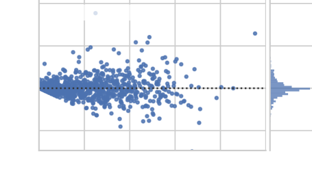
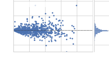
Tab. 3 and Tab. 4 presents the results on the training and validation set, respectively. Note that the models using extracted features (linear regression, power regression, and RF) were trained on the union of training and validation set, while our point cloud regression models were not. Still, the more recent models directly working on the point cloud data consistently produced better results. Fig. 11 and 12 illustrate residual plots and error distribution of biomass and wood volume, respectively, which completes Fig. 7.
In Fig. 13 we show more subplots with particularly low or high values for above-ground biomass. For example, the first two subplots have low AGB with and Mg ha-1, which is reflected by the sparse vegetation in the point cloud. This is difficult to capture with commonly used statistics derived from point cloud data, and therefore models based on these features (e.g., RF, lin., and power model) overestimated. Interestingly, PointNet also overestimate values due to the employed global aggregation without intermediate downsampling steps (similar to global feature extraction). The third example in Fig. 13 exhibits a high AGB value with Mg ha-1 and the point cloud shows a densely populated and natural broadleaf forest. Again, this is difficult to estimate since the derived statistics do not offer information about individual biomass contributions and thus most methods underestimate them. The fourth subplots biomass is Mg ha-1 from a conifer forest and the predictions align well with the target. We also give a visualization of the plots and subplots in Fig. 14 (as described in Sec. 2.1).
| RMSE | MAPE | ||||||
|---|---|---|---|---|---|---|---|
| target | model | med. | max | med. | min | med. | min |
| AGB | linear | ||||||
| power | |||||||
| RF | |||||||
| PointNet | |||||||
| KPConv | |||||||
| MSENet14 | |||||||
| MSENet50 | |||||||
| volume | linear | ||||||
| power | |||||||
| RF | |||||||
| PointNet | |||||||
| KPConv | |||||||
| MSENet14 | |||||||
| MSENet50 | |||||||

| linear |
| power |
| RF |
| PointNet |
| KPConv |
| MSENet14 |
| MSENet50 |
| 0.0 |
| 0.2 |
| 0.4 |
| 0.6 |
| 0.8 |
| 0 |
| (0, 33] |
| (33, 66] |
| (66, 100) |
| 100 |
conifer fraction
| 0 |
| 50 |
| 25 |
| 75 |
| 100 |
| RMSE |
| 0 |
| 200 |
| 400 |
| 600 |
| 800 |
| MAPE |
| mean error: 1.34 Mg ha-1 |
| 0 |
| 100 |
| 200 |
| 300 |
| 400 |
| 500 |
| predicted AGB |
| -200 |
| 0 |
| 200 |
| 400 |
residuals
| mean error: 1.56 Mg ha-1 |
| 0 |
| 100 |
| 200 |
| 300 |
| 400 |
| 500 |
| predicted AGB |
| -200 |
| 0 |
| 200 |
| 400 |
residuals
| mean error: 1.49 Mg ha-1 |
| 0 |
| 100 |
| 200 |
| 300 |
| 400 |
| 500 |
| predicted AGB |
| -200 |
| 0 |
| 200 |
| 400 |
residuals
| mean error: 0.17 Mg ha-1 |
| 0 |
| 100 |
| 200 |
| 300 |
| 400 |
| 500 |
| predicted AGB |
| -200 |
| 0 |
| 200 |
| 400 |
residuals
| mean error: 4.50 m3 ha-1 |
| 0 |
| 200 |
| 400 |
| 600 |
| 800 |
| 1000 |
| predicted volume |
| -500 |
| -250 |
| 0 |
| 250 |
| 500 |
| 750 |
residuals
| mean error: 3.46 m3 ha-1 |
| 0 |
| 200 |
| 400 |
| 600 |
| 800 |
| 1000 |
| predicted volume |
| -500 |
| -250 |
| 0 |
| 250 |
| 500 |
| 750 |
residuals
| mean error: 4.22 m3 ha-1 |
| 0 |
| 200 |
| 400 |
| 600 |
| 800 |
| 1000 |
| predicted volume |
| -500 |
| -250 |
| 0 |
| 250 |
| 500 |
| 750 |
residuals
| mean error: 3.24 m3 ha-1 |
| 0 |
| 200 |
| 400 |
| 600 |
| 800 |
| 1000 |
| predicted volume |
| -500 |
| -250 |
| 0 |
| 250 |
| 500 |
| 750 |
residuals
| mean error: 1.64 m3 ha-1 |
| 0 |
| 200 |
| 400 |
| 600 |
| 800 |
| 1000 |
| predicted volume |
| -500 |
| -250 |
| 0 |
| 250 |
| 500 |
| 750 |
residuals
| mean error: 2.34 m3 ha-1 |
| 0 |
| 200 |
| 400 |
| 600 |
| 800 |
| 1000 |
| predicted volume |
| -500 |
| -250 |
| 0 |
| 250 |
| 500 |
| 750 |
residuals
| mean error: 1.83 m3 ha-1 |
| 0 |
| 200 |
| 400 |
| 600 |
| 800 |
| 1000 |
| predicted volume |
| -500 |
| -250 |
| 0 |
| 250 |
| 500 |
| 750 |
residuals
