A Discontinuous Galerkin Solver in the FLASH Multi-Physics Framework

Abstract

In this paper, we present a discontinuous Galerkin solver based on previous work by the authors for magneto-hydrodynamics in form of a new fluid solver module integrated into the established and well-known multi-physics simulation code FLASH. Our goal is to enable future research on the capabilities and potential advantages of discontinuous Galerkin methods for complex multi-physics simulations in astrophysical settings. We give specific details and adjustments of our implementation within the FLASH framework and present extensive validations and test cases, specifically its interaction with several other physics modules such as (self-)gravity and radiative transfer. We conclude that the new DG solver module in FLASH is ready for use in astrophysics simulations and thus ready for assessments and investigations.

1 Introduction

In astrophysics, numerical simulations are a standard tool to study the interplay of the complex physical processes which are shaping our universe. As an example, understanding the star formation process requires numerical simulations because the process is too slow to be followed in real time and the star-forming gas is so dense that the young stellar objects are highly obscured and cannot be directly observed. The star formation process involves compressible fluid dynamics with magnetic fields and strong shocks, self-gravity of the gas, heating and cooling, multi-component chemistry, and radiative transfer. It is therefore a challenging, multi-physics problem and requires accurate as well as stable numerical methods and scalable high-performance computing implementations.

There are many (open source) code frameworks in the astrophysics community that include (a subset of) the aforementioned physical models with different fidelity levels. A few examples are AREPO (Springel, 2010), RAMSES (Fromang et al., 2006), ENZO (Collins et al., 2010), Dedalus (Burns et al., 2020), ATHENA (Stone et al., 2008), ATHENA++ (Stone et al., 2020), ORION2 (Li et al., 2021), and the FLASH code (Fryxell et al., 2000). Here, we list code frameworks that are based on discretisations with meshes, as this strategy is also the focus of this paper. Most of these codes feature adaptive mesh refinement (AMR), which is crucial to resolve the vastly different spatial scales in the turbulent interstellar medium. Furthermore, most of these codes are based on Finite Volume (FV) type discretisations of the fluid/plasma dynamics with numerical fluxes based on Riemann solvers at the interface and, typically, second order reconstructions with slope limiting to increase the accuracy by decreasing artificial dissipation. In general, FV methods are quite effective and robust and they are able to handle strong shocks. Thus, they are currently the state-of-the-art in almost all grid-based multi-physics astrophysical simulation codes.

High-order discretisation schemes (e.g. Balsara, 2017) promise a higher fidelity and precision while being computationally efficient. This is attractive since most astrophysical simulations are notoriously under-resolved due to limited computing resources and/or parallel scalability of the employed methods. While there are many high-order methodologies available, this paper focuses on discontinuous Galerkin (DG) schemes. DG schemes are a mixture of high-order Finite Element methods with local polynomial basis functions and FV methods in the sense that the ansatz space is discontinuous across grid cell interfaces, which enables the use of Riemann solver based numerical fluxes.

The goal to efficiently make use of future exascale machines with their ever higher degree of parallel concurrency motivates the search for more efficient and more accurate techniques for computing hydrodynamics. DG methods can be straightforwardly extended to arbitrarily high order of accuracy while requiring only minimal data from adjacent neighbours. Thus, the DG scheme has a very narrow data dependency with only a minimum of data exchange necessary, while the local compute kernels are computationally very dense. Furthermore, at least for subsonic turbulence, high-order DG offers significant computational benefits in computational efficiency for reaching a desired target accuracy, due to their spectral like very low dispersion and dissipation errors (e.g. Ainsworth, 2004; Gassner & Kopriva, 2011; Dobrev et al., 2012; He et al., 2020). Low artificial dissipation is important to reduce artificial damping and heating, in addition, low dispersion errors are equally important as it guarantees high accuracy for wave propagation and interaction. Last but not least, DG method intrinsically conserve angular momentum for approximation order 3 and higher (Després & Labourasse, 2015).

These beneficial properties of DG are the reason why applications in engineering are very successful (e.g. Bassi et al., 2005; Zhang & Stanescu, 2010; Moura et al., 2017; Manzanero et al., 2018), where mainly weakly compressible turbulent flows in complex geometries are simulated. However, their application in astrophysics for hypersonic flows is still in an early stage. DG methods with focus on astrophysical fluid dynamics and related applications are for instance presented in Schaal et al. (2015); Guillet et al. (2019); Bauer et al. (2016); Kidder et al. (2017); Lombart & Laibe (2020); Mocz et al. (2014).

However, to the best of our knowledge, there is no DG implementation in a full production multi-physics framework available up to now. The scientific contribution of this paper is to integrate a DG solver into an existing and well-known multi-physics simulation code to enable research on the capabilities and potential advantages of DG for complex multi-physics simulations in astrophysical settings. Here we choose the FLASH code (Fryxell et al., 2000).

To allow the robust simulation of highly supersonic, turbulent flows featuring strong shocks, as is the case in most astrophysics models, proper shock capturing for DG is mandatory. There are many shock capturing approaches available in the DG literature, for instance based on slope limiters Cockburn & Shu (1998); Cockburn et al. (1990); Kuzmin (2012) or (H)WENO limiters Guo et al. (2015); Qiu & Zhu (2010); Zhu & Qiu (2009), filtering Bohm et al. (2019), and artificial viscosity Persson & Peraire (2006); Ching et al. (2019). Sub-cell based FV discretisations with a first order, second order TVD or high order WENO reconstruction are introduced, e.g., in Vilar (2019); Sonntag & Munz (2014); Dumbser et al. (2014); Zanotti et al. (2015); Dumbser & Loubere (2016).

Markert et al. (2021) introduced a shock capturing approach for high-order DG which has shown to be robust under very strong astrophysical shock conditions (with large density and pressure contrasts), while retaining the beneficial properties of DG as much as possible and keeping physical quantities, like density and pressure, positive. As a side note, but important detail, the method of Markert et al. (2021) is directly compatible with FLASH’s block-based datastructure, and serves as a baseline approach for the current paper.

In the remainder of the paper we briefly discuss the governing equations used for the DG implementation, as well as the specific details and adjustments of the DG scheme by Markert et al. (2021) that we have implemented in the FLASH code. We then present extensive validations of the DG scheme and specifically its interaction with several multi-physics modules. The idea is that we increase the complexity of the test cases step by step, where the last test case in Section 5.5.2 is a more involved multi-physics astrophysics application with multiple physics modules working together.

2 Governing Equations

We assume that the magnetised plasma in our astrophysical applications is described reasonably by the equations of ideal magneto-hydrodynamics (iMHD)

$$\partial_{t}\begin{pmatrix}\rho\\ \rho\vec{v}\\ E\\ \vec{B}\end{pmatrix}+\nabla\cdot\begin{pmatrix}\rho\vec{v}\\ \rho\vec{v}\otimes\vec{v}+P\mathcal{I}-\vec{B}\otimes\vec{B}\\ (E+P)\vec{v}-(\vec{v}\cdot\vec{B})\vec{B}\\ \vec{B}\otimes\vec{v}-\vec{v}\otimes\vec{B}\end{pmatrix}=0,$$ (1)

where $\rho$ is the density, $\vec{v}=(v_{1},v_{2},v_{3})^{T}$ is the velocity, $E$ is the total energy, $\vec{B}=(B_{1},B_{2},B_{3})^{T}$ is the magnetic field, $\mathcal{I}$ represents the $3\times 3$ identity matrix and the total pressure $P$:

$$P=p+\frac{1}{2}\vec{B}\cdot\vec{B}.$$ (2)

The thermal pressure $p$ is given in equation (5).

A crucial property of magnetic fields is that their divergence is exactly zero for all times. Numerically, it is challenging to exactly satisfy this condition (e.g. Brackbill & Barnes, 1980; Evans & Hawley, 1988; Ryu et al., 1998; Balsara & Spicer, 1999; Gardiner & Stone, 2005; Dedner et al., 2002). In this work, we focus on an extension of the iMHD equations, that accounts for the inexact divergence of the magnetic field by introducing a generalised Lagrange multiplier (GLM), i.e., an additional equation that "carries" the divergence error following the work of Dedner et al. (2002). However, we focus on a specific variant of the GLM extension, that is entropy consistent and consistent with the Lorentz force (Derigs et al., 2018; Bohm et al., 2018). In the present implementation, we have further extended the MHD model to allow for multiple components, necessary for the complex chemistry network interactions.

2.1 Ideal Generalised Lagrange Multiplier MHD

The form of the ideal generalised Lagrange multiplier magneto-hydrodynamics (iGLM-MHD), extended for multiple chemical species and coupled to the gravity source term reads as

$$\partial_{t}\boldsymbol{u}+\partial_{x}\boldsymbol{F}(\boldsymbol{u})+\partial_{y}\boldsymbol{G}(\boldsymbol{u})+\partial_{z}\boldsymbol{H}(\boldsymbol{u})=-\boldsymbol{\Upsilon}^{\text{Powell}}-\boldsymbol{\Upsilon}^{\text{GLM}}+\boldsymbol{\Upsilon}^{\text{gravity}}.$$ (3)

The vector of state variables (typeface in bold) consists of

$$\boldsymbol{u}=(\rho,\;\rho\,\vec{v},\;E,\;\vec{B},\;\Psi,\;\rho\,\boldsymbol{\sigma})^{T}\quad\in\mathbb{R}^{9+n},$$ (4)

with the addition of the hyperbolic divergence correction field $\Psi$ and the species vector $\boldsymbol{\sigma}=(\sigma_{1},\ldots,\sigma_{n})^{T}$ describing mass fractions of the $n$ different chemical species. The thermal pressure, $p$, is computed from the total energy via

$$p=(\gamma-1)\Big{(}E-\frac{\rho}{2}\vec{v}\cdot\vec{v}-\frac{1}{2}\vec{B}\cdot\vec{B}-\frac{1}{2}\Psi^{2}\Big{)},$$ (5)

where the heat capacity ratio, $\gamma$, is given by (8). The flux in x-direction reads as

$$\boldsymbol{F}=\left(\begin{matrix}\rho v_{1}\\[3.99994pt] \rho v_{1}v_{1}+p+\frac{1}{2}\vec{B}\cdot\vec{B}-B_{1}B_{1}\\[3.99994pt] \rho v_{1}v_{2}-B_{1}B_{2}\\[3.99994pt] \rho v_{1}v_{3}-B_{1}B_{3}\\[3.99994pt] v_{1}\big{(}\frac{\rho}{2}\vec{v}\cdot\vec{v}+\frac{\gamma\,p}{\gamma-1}+\vec{B}\cdot\vec{B}\big{)}-B_{1}\,\vec{v}\cdot\vec{B}+c_{h}\Psi B_{1}\\[3.99994pt] c_{h}\Psi\\[3.99994pt] v_{1}B_{2}-v_{2}B_{1}\\[3.99994pt] v_{1}B_{3}-v_{3}B_{1}\\[3.99994pt] c_{h}B_{1}\\[3.99994pt] \rho v_{1}\boldsymbol{\sigma}\end{matrix}\right)\in\mathbb{R}^{9+n},$$ (6)

with the hyperbolic correction speed $c_{h}$ given by eq. (17). The fluxes in $y$- and z-direction, respectively $G$ and $H$, are listed in Derigs et al. (2018) Appendix F, yet without the multi-species extension.

What follows is a detailed discussion of the different parts of the governing equations: quasi-multi-fluids, maximum wave speeds, Powell source terms $\boldsymbol{\Upsilon}^{\text{Powell}}$ and the hyperbolic divergence cleaning technique with its associated source term $\boldsymbol{\Upsilon}^{\text{GLM}}$.

2.1.1 Quasi-multi-fluid Model

The ability to track the exact composition of a fluid or gas is of central importance in astrophysical simulations as they include detailed chemical reaction chains (chemical networks) to treat heating, cooling, as well as the formation and destruction of chemical compounds in order to mimic the behaviour of the interstellar medium (ISM; Walch et al., 2015; Gatto et al., 2015; Glover & Clark, 2014). The individual species are traced by mass fractions $\sigma_{s}\in[0,1]$, which all move with the same velocity $\vec{v}$ as the total density $\rho$:

$$\partial_{t}(\rho\,\sigma_{s})+\nabla\cdot(\rho\,\vec{v}\,\sigma_{s})=0,\quad s=1,\ldots,n.$$ (7)

The sum of all $n$ mass fractions maintains the total density at all times, i.e. $\sum_{s}^{n}\sigma_{s}=1$.

We generalise our scheme for a multi-species fluid with a variable heat capacity ratio $\gamma$ by adopting a weighted mean over all species (Murawski, 2002):

$$\gamma=\frac{\sum_{s}^{n}c^{\text{pres.}}_{s}\,\sigma_{s}}{\sum_{s}^{n}c^{\text{vol.}}_{s}\,\sigma_{s}}$$ (8)

with the heat capacities for constant pressure $c^{\text{pres.}}_{s}$ and constant volume $c^{\text{vol.}}_{s}$ of each individual species. The standard FLASH framework readily offers inbuilt multi-species support with modules taking care of the correct equation-of-state calculations (8). It considerably minimises the implementation effort on our side by only focusing on the proper species advection part.

In addition to the multi-fluid approach, we also support mass tracer fields (also called mass scalars) which are advected similar to (7). The implementation of the tracer fields allows the use of any number of such fields which makes it a flexible tool for tracing different mass quantities according to individual requirements. For example, a mass tracer field could be used to follow the distribution of metals in the interstellar gas with virtually no additional costs. Note, that we do not include mass tracer fields explicitly in (4) since they do not involve any special numerical discretisation than already presented here.

2.1.2 Maximum Wave Speed

A vital step in our numerical treatment of iGLM-MHD is to compute the maximum eigenvalue of the system. It encodes the maximum wave speed involved in the solution and helps to find a good estimation for an acceptable timestep in case of explicit time integration. A thorough investigation of the full eigenvalue system is presented in Derigs et al. (2018). In this work, we focus on the fastest signal called the fast magneto-sonic wave speed. In direction $d=1,2,3$ it is calculated as

$$c_{d}=\frac{\sqrt{c_{\text{sound}}^{2}+c_{\text{Alfv\'{e}n}}^{2}+\sqrt{(c_{\text{sound}}^{2}+c_{\text{Alfv\'{e}n}}^{2})^{2}-(2\,c_{\text{sound}}B_{d}/\sqrt{\rho})^{2}}}}{\sqrt{2}},$$ (9)

where the sonic wave speed and Alfvén wave speed read

$$c_{\text{sound}}=\sqrt{\gamma\,\frac{p}{\rho}}\quad\text{and}\quad c_{\text{Alfv\'{e}n}}=\frac{|\vec{B}|}{\sqrt{\rho}}.$$ (10)

The upper bound of all involved wave speeds in direction $d=1,2,3$ is then given by

$$\lambda^{\text{max}}_{d}=\big{|}v_{d}\big{|}+c_{d}.$$ (11)

2.1.3 Powell Source Terms

Following the theoretical groundwork by Godunov (1972), Powell et al. (1999) pointed out that the system (1) is not Galilean invariant and does not formally conserve entropy. They proposed to add a specific source term proportional to $\nabla\cdot B$ in order to symmetrize the system. The so-called Powell terms can be obtained from deriving the local form of the system (1) based on integral conservation laws (Powell et al., 1999) or from requiring entropy stability (Godunov, 1972; Winters & Gassner, 2016; Chandrashekar & Klingenberg, 2016; Derigs et al., 2018).

We write the Powell source terms in eq. (3) as

$$\boldsymbol{\Upsilon}^{\text{Powell}}=\big{(}\partial_{x}B_{1}+\partial_{y}B_{2}+\partial_{z}B_{3}\big{)}\;\boldsymbol{\Phi}^{\text{Powell}}\quad\text{with}$$ (12)

$$\boldsymbol{\Phi}^{\text{Powell}} =\big{(}0,\;\vec{B},\;\vec{v}\cdot\vec{B},\;\vec{v},\;0,\;\boldsymbol{0}\big{)}^{T}\quad\in\mathbb{R}^{9+n}.$$ (13)

The Powell method can be easily adapted to Eulerian grid codes (Balsara & Spicer, 1999; Tóth, 2000). It has been successfully implemented and tested in astrophysical MHD codes equipped with a FV scheme and AMR (Derigs et al., 2016). For DG it is for instance adopted by Warburton & Karniadakis (1999) and Bohm et al. (2018) for viscous and resistive MHD flows.

The Powell method has two limitations. Firstly, it does not fully eliminate the divergence error and can result in a local accumulation of numerical divergence in regions of stagnant flows. Secondly, the source term is not strictly conservative anymore since it will locally inject conserved quantities in the presence of numerical divergence errors. We investigate these issues in the numerical results in Section 5.2.2 and argue that the combination with hyperbolic divergence cleaning, discussed in the next paragraph, remedies these issues and leads to acceptable results.

2.1.4 Hyperbolic Divergence Cleaning

Munz et al. (2007) coupled the divergence constraint for the electric field with the induction equation by introducing a generalised Lagrangian multiplier (GLM), $\Psi$, as an additional field. As in Dedner et al. (2002), we apply this technique to iMHD in order to account for the divergence-free condition $\nabla\cdot B=0$ by adding the GLM $\Psi$ as another conservative state variable, which we call hyperbolic divergence correction field. This new field couples to the divergence of the magnetic field through a modified induction equation (Derigs et al., 2018):

$$\partial_{t}\vec{B}+\nabla\cdot(\vec{B}\otimes\vec{v}-\vec{v}\otimes\vec{B})+\nabla\cdot\Psi=0.$$

The field $\Psi$ evolves via the dynamical equation

$$\partial_{t}\Psi+c_{h}\nabla\cdot\vec{B}+\vec{v}\,\nabla\Psi+c_{p}\Psi=0,$$

resulting in a coupled GLM-iMHD system, which makes the fluctuations of $\Psi$ propagate away from their sources at speed $c_{h}>0$ while damping them with the damping speed $c_{p}>0$ at time-scales $\propto c_{h}^{-1}$.

We write the GLM source terms in eq. (3) as

$$\boldsymbol{\Upsilon}^{\text{GLM}}=\big{(}v_{1}\;\partial_{x}\Psi+v_{2}\;\partial_{y}\Psi+v_{3}\;\partial_{z}\Psi\big{)}\;\boldsymbol{\Phi}^{\text{GLM}}+c_{p}\,\boldsymbol{\Phi}^{\text{damp}},$$ (14)

with GLM vectors

$$\boldsymbol{\Phi}^{\text{GLM}} =\big{(}0,\;\vec{0},\;\Psi,\;\vec{0},\;1,\;\boldsymbol{0}\big{)}^{T}\in\mathbb{R}^{9+n}\quad\text{and}$$ (15)

$$\boldsymbol{\Phi}^{\text{damp}} =\big{(}0,\;\vec{0},\;0,\;\vec{0},\;\Psi,\;\boldsymbol{0}\big{)}^{T}\in\mathbb{R}^{9+n}.$$ (16)

For efficient divergence propagation without compromising stability we set $c_{h}$ to be the maximum magneto-sonic wave speed (see eq. (9)) present in the entire physical domain $\Omega$:

$$c_{h}=\max_{\Omega}\max_{d=1}^{3}c_{d}.$$ (17)

According to Dedner et al. (2002) a good choice for the damping speed, $c_{p}$, is given by

$$c_{p}=\frac{c_{h}}{0.18}.$$

The GLM method is straightforward to implement in existing schemes and it has also been adopted by a number of MHD codes (Gaburov & Nitadori, 2011; Mignone et al., 2012; dumbser2016simple; Bohm et al., 2018; Rueda-Ramírez et al., 2021).

2.1.5 Coupling to Gravity

The inclusion of gravity in the governing equations introduces a force on the right-hand side of the momentum equations of the form

$$\partial_{t}(\rho\vec{v})+\rho\nabla\phi=0,$$

where the gravitational potential $\phi$ satisfies the Poisson equation

$$\nabla^{2}\phi=4\pi\,G\,\rho,$$

with gravitational constant $G$. The source term in eq. (3) then reads

$$\boldsymbol{\Upsilon}^{\text{gravity}}=\big{(}0,\;\rho\,\vec{g},\;\rho\,\vec{v}\cdot\vec{g},\;\vec{0},\;0,\;\boldsymbol{0}\big{)}^{T}\in\mathbb{R}^{9+n},$$ (18)

with the gravitational acceleration $\vec{g}=(g_{1},g_{2},g_{3})^{T}$. The gravity accelerations are computed with any of the gravity solvers available in the FLASH framework (e.g. Wünsch et al., 2018). We expand on available gravity solvers in Section 5.4.

3 Numerical Discretisation

In this section, we give a brief description of our numerical discretisation of the system given in eq. (3). We employ a newly developed DG variant based on blocks of mean values (Markert et al., 2021). This enables us to construct a shock capturing approach based on the idea that we use high-order DG whenever possible, whereas we blend the scheme with a second-order slope limiting FV scheme when there are for instance strong shocks.

The standard solver in FLASH is based on an AMR enabled second-order FV method, where the fluid variables are stored in the form of mean values. FLASH organises by default the FV mean values in blocks of specific sizes, e.g., of size $8\times 8\times 8$. It is important to note, that all other physics modules of FLASH assume that the data is organised in form of such blocks with mean values and hence that the interaction between the additional physics modules and the FLASH fluid solvers is based on mean values. In contrast, typically, in DG the fluid variables are stored in form of local polynomials with either modal coefficients (Karniadakis & Sherwin, 2005) or nodal values (Kopriva, 2009). Depending on the polynomial degree $N-1$ of the local ansatz, $N^{3}$ unknowns per fluid variable form a data package. Thus, the size of the blocks (or in DG jargon size of the "elements"), varies with the choice of the polynomial degree.

This difference in the representation of the solutions and the interpretation of the solution coefficients forms a tough challenge that needs to be overcome. Roughly, we have to major choices: (i) We can implement the DG scheme in its typical/natural form based on the polynomial representations. This means, however, that we than need to adjust the whole FLASH code to cater to the piece-wise polynomial data. Thus, changes in the way the grid is managed (not blocks of constant size, but smaller elements) and changes in the way all other physics modules interact with the DG solver have to be changed and implemented. (ii) We adapt the DG methodology and specifically design a variant that directly operates with the block based mean value data structure of FLASH. The upside is of course that in this case DG can with reasonable implementation effort directly access all the functionality that the FLASH code offers. The downside is that this is not the "natural" way one would implement the DG methodology and that there are thus some disadvantages, such as additional transforms between ansatz spaces, that one needs to accept.

In this paper, we have decided in favour of option (ii), where we adjust the DG methodology such that we can directly use the rich multi-physics framework that FLASH offers. In previous work, we have presented a robust and accurate DG variant that uses blocks of mean values as input (Markert et al., 2021), which serves as a starting reference for the FLASH implementation.

Besides option (ii) being presumably the only feasible approach regarding the necessary amount of implementation, it further has beneficial effects such as being able to directly use the post-processing tool chains for data organised in blocks of mean values, which have been established in many years of research work.

We first introduce the notations for FV and DG separately, and then we combine both schemes via convex blending. We also highlight our solution to make the two schemes compatible within the FLASH framework while maintaining the key numerical properties such as conservation and accuracy. We conclude this section with a short discussion about the employed time integration method and how we enforce positivity of density and pressure.

3.1 Finite Volume Scheme

We assume a Cartesian grid and subdivide the physical domain $\Omega$ into $Q$ blocks, each consisting of $N\times N\times N$ regular sub-cells of size

$$\left(\frac{\Delta x_{q}}{N},\frac{\Delta y_{q}}{N},\frac{\Delta z_{q}}{N}\right)^{T}=:\frac{\Delta\vec{x}_{q}}{N}.$$

Each sub-cell of block $q$ represents the cell-averaged fluid state $\boldsymbol{u}(t,\vec{x})$ at sub-cell centres $\vec{x}=\vec{\mu}_{q,ijk}$ and time $t$:

$$\overline{\boldsymbol{u}}_{q,ijk}(t)=\frac{N^{3}}{\Delta x_{q}\,\Delta y_{q}\,\Delta z_{q}}\iiint_{\vec{\mu}_{q,ijk}-\frac{\Delta\vec{x}_{q}}{2\,N}}^{\vec{\mu}_{q,ijk}+\frac{\Delta\vec{x}_{q}}{2\,N}}\boldsymbol{u}(t,\vec{x})\,dxdydz,$$ (19)

with $i,j,k=1,\ldots,N$. For the sake of brevity, we do not declare the range of indices $i,j,k$ in each equation from here on. Furthermore, we write a bar over each quantity that represents a cell-averaged or face-averaged mean value.

Following the standard procedure (Toro, 1999), we construct within each block $q$ a three-dimensional FV scheme. In semi-discrete form it reads

$$\partial_{t}\overline{\boldsymbol{u}}_{q,ijk}^{\text{FV}}= -\frac{N}{\Delta x_{q}}\big{(}\overline{\boldsymbol{F}}^{*}_{q,i+\frac{1}{2}jk}-\overline{\boldsymbol{F}}^{*}_{q,i-\frac{1}{2}jk}\big{)}$$

$$-\frac{N}{\Delta y_{q}}\big{(}\overline{\boldsymbol{G}}^{*}_{q,ij+\frac{1}{2}k}-\overline{\boldsymbol{G}}^{*}_{q,ij-\frac{1}{2}k}\big{)}$$

$$-\frac{N}{\Delta z_{q}}\big{(}\overline{\boldsymbol{H}}^{*}_{q,ijk+\frac{1}{2}}-\overline{\boldsymbol{H}}^{*}_{q,ijk-\frac{1}{2}}\big{)}$$

$$-\overline{\boldsymbol{\Upsilon}}^{\text{Powell}}_{q,ijk}-\overline{\boldsymbol{\Upsilon}}^{\text{GLM}}_{q,ijk}.$$ (20)

The consistent numerical flux $\boldsymbol{F}^{*}$ has the general form

$$\overline{\boldsymbol{F}}^{*}_{q,i+\frac{1}{2}jk}=\boldsymbol{F}^{*}\big{(}\boldsymbol{u}^{+}_{q,i+\frac{1}{2}jk},\boldsymbol{u}^{-}_{q,i+\frac{1}{2}jk}\big{)}$$ (21)

$$\>=\boldsymbol{F}^{\text{KEPEC}}\big{(}\boldsymbol{u}^{+}_{q,i+\frac{1}{2}jk},\boldsymbol{u}^{-}_{q,i+\frac{1}{2}jk}\big{)}-\text{{Stab}}\big{(}\boldsymbol{u}^{+}_{q,i+\frac{1}{2}jk},\boldsymbol{u}^{-}_{q,i+\frac{1}{2}jk}\big{)},$$

where $\boldsymbol{F}^{\text{KEPEC}}$ is a kinetic energy and entropy conserving (KEPEC) two-point flux derived in Derigs et al. (2018). The interface values $\boldsymbol{u}^{+}$ and $\boldsymbol{u}^{-}$ are retrieved from a total variation diminishing (TVD) reconstruction method. A thorough discussion about time-proven reconstruction methods can be found in Toro (1999).

In order to introduce dissipation the numerical flux is subtracted with a stabilisation term Stab. In this work we use the simple and very robust Rusanov-type dissipation:

$$\overline{\boldsymbol{F}}^{*}_{q,i+\frac{1}{2}jk}=\overline{\boldsymbol{F}}^{\text{KEPEC}}_{q,i+\frac{1}{2}jk}-\frac{1}{2}\lambda^{\text{max}}_{q,i+\frac{1}{2}jk}\Big{(}\boldsymbol{u}^{+}_{q,i+\frac{1}{2}jk}-\boldsymbol{u}^{-}_{q,i+\frac{1}{2}jk}\Big{)},$$ (22)

with

$$\lambda^{\text{max}}_{q,i+\frac{1}{2}jk}=\max\Big{\{}\lambda^{\text{max}}_{1}(\boldsymbol{u}^{+}_{q,i+\frac{1}{2}jk}),\;\lambda^{\text{max}}_{1}(\boldsymbol{u}^{-}_{q,i+\frac{1}{2}jk})\Big{\}}$$

being the maximum wave speed (11) at the interface. Since the KEPEC flux in Derigs et al. (2018) is not specified for multiple species we resort to the following advection scheme

$$\overline{\boldsymbol{F}}^{*,\text{species}}_{q,i+\frac{1}{2}jk}=\left\{\left\{\rho v_{1}\boldsymbol{\sigma}\right\}\right\}_{q,i+\frac{1}{2}jk}-\frac{1}{2}\lambda^{\text{max}}_{q,i+\frac{1}{2}jk}\left[\left[\rho\boldsymbol{\sigma}\right]\right]_{q,i+\frac{1}{2}jk}.$$ (23)

To allow a succinct notation we introduce the mean and jump operators, respectively,

$$\left\{\left\{\cdot\right\}\right\}_{q,i+\frac{1}{2}jk} =\frac{1}{2}\Big{(}(\cdot)^{+}_{q,i+\frac{1}{2}jk}+(\cdot)^{-}_{q,i+\frac{1}{2}jk}\Big{)},\quad\text{and}$$ (24)

$$\left[\left[\cdot\right]\right]_{q,i+\frac{1}{2}jk} =(\cdot)^{-}_{q,i+\frac{1}{2}jk}-(\cdot)^{+}_{q,i+\frac{1}{2}jk}.$$ (25)

The fluxes $\boldsymbol{G}^{*}$ and $\boldsymbol{H}^{*}$ are defined analogously.

The gradients in the Powell term (12) are approximated with central finite differencing over sub-cell $\overline{\boldsymbol{u}}_{q,ijk}$. In x-direction we write

$$\overline{\boldsymbol{\Upsilon}}^{\text{Powell},x}_{q,ijk}=\frac{N}{\Delta x_{q}}\Big{(}\left\{\left\{B_{1}\right\}\right\}_{q,i+\frac{1}{2}jk}-\left\{\left\{B_{1}\right\}\right\}_{q,i-\frac{1}{2}jk}\Big{)}\;\overline{\boldsymbol{\Phi}}^{\text{Powell}}_{q,ijk},$$ (26)

where the source vector is calculated by inserting the mean values into expression (13): $\overline{\boldsymbol{\Phi}}^{\text{Powell}}_{q,ijk}:=\boldsymbol{\Phi}^{\text{Powell}}\big{(}\overline{\boldsymbol{u}}_{q,ijk}\big{)}$. The complete flux is then the sum along all directions

$$\overline{\boldsymbol{\Upsilon}}^{\text{Powell}}_{q,ijk}=\overline{\boldsymbol{\Upsilon}}^{\text{Powell},x}_{q,ijk}+\overline{\boldsymbol{\Upsilon}}^{\text{Powell},y}_{q,ijk}+\overline{\boldsymbol{\Upsilon}}^{\text{Powell},z}_{q,ijk}.$$

The discretisation of the GLM term (12) is done analogously and reads

$$\overline{\boldsymbol{\Upsilon}}^{\text{GLM},x}_{q,ijk}=v_{1}\;\frac{N}{\Delta x_{q}}\Big{(}\left\{\left\{\psi\right\}\right\}_{q,i+\frac{1}{2}jk}-\left\{\left\{\psi\right\}\right\}_{q,i-\frac{1}{2}jk}\Big{)}\;\overline{\boldsymbol{\Phi}}^{\text{GLM}}_{q,ijk}.$$ (27)

The complete flux is the sum along all directions and the damping term:

$$\overline{\boldsymbol{\Upsilon}}^{\text{GLM}}_{q,ijk}=\overline{\boldsymbol{\Upsilon}}^{\text{GLM},x}_{q,ijk}+\overline{\boldsymbol{\Upsilon}}^{\text{GLM},y}_{q,ijk}+\overline{\boldsymbol{\Upsilon}}^{\text{GLM},z}_{q,ijk}+c_{p}\overline{\boldsymbol{\Phi}}^{\text{damp}}_{q,ijk}.$$

3.2 Discontinuous Galerkin Spectral Element Method

Similar to the previous section we assume a Cartesian grid and subdivide the physical domain $\Omega$ into $Q$ elements of size

$$\left(\Delta x_{q},\Delta y_{q},\Delta z_{q}\right)^{T}=:\Delta\vec{x}_{q}.$$

Inside each element $q$ we make a polynomial tensor product ansatz of degree $N-1$ and approximate the exact solution $\boldsymbol{u}(t,\vec{x})$ by

$$\boldsymbol{u}\big{(}t,\vec{x}_{q}(\vec{\chi})\big{)}\approx\sum^{N}_{ijk=1}\boldsymbol{u}\big{(}t,\vec{x}_{q}(\vec{\xi}_{ijk})\big{)}\;\ell_{i}(\chi_{1})\ell_{j}(\chi_{2})\ell_{k}(\chi_{3}),$$ (28)

where $\vec{x}_{q}(\vec{\chi})=\vec{\mu}_{q}+\vec{\chi}\,\Delta\vec{x}_{q}\in\Omega$ is a mapping from reference space $\vec{\chi}\in\big{[}-\frac{1}{2},\frac{1}{2}\big{]}^{3}$ to the physical domain anchored around the element’s midpoint $\vec{\mu}_{q}$. The Lagrange polynomials $\ell_{i},\ell_{j},\ell_{k}$ are pinned to the Legendre-Gauss quadrature nodes

$$\vec{\xi}_{ijk}=(\xi_{i},\xi_{j},\xi_{k})^{T}\in\Big{[}-\frac{1}{2},\frac{1}{2}\Big{]}^{3},\quad i=1,\ldots,N.$$ (29)

The associated quadrature weights, $\omega_{i}\in\big{(}0,1\big{)}$, fulfil $\sum^{N}_{i}\omega_{i}=1$.

Following the standard procedure in Kopriva (2009), we get the semi-discrete weak-form

$$\partial_{t}\widetilde{\boldsymbol{u}}_{q,ijk}^{\text{DG}}=$$ (30)

$$\quad-\frac{1}{\omega_{i}\,\Delta x_{q}}\Big{(}\mathcal{B}^{+}_{i}\,\widetilde{\boldsymbol{F}}^{*}_{q+\frac{1}{2},jk}-\mathcal{B}^{-}_{i}\,\widetilde{\boldsymbol{F}}^{*}_{q-\frac{1}{2},jk}-\sum^{N}_{l=1}\omega_{l}\,\mathcal{D}_{li}\,\widetilde{\boldsymbol{F}}_{q,ljk}\Big{)}$$

$$\quad-\frac{1}{\omega_{j}\,\Delta y_{q}}\Big{(}\mathcal{B}^{+}_{j}\,\widetilde{\boldsymbol{G}}^{*}_{q+\frac{1}{2},ik}-\mathcal{B}^{-}_{j}\,\widetilde{\boldsymbol{G}}^{*}_{q-\frac{1}{2},ik}-\sum^{N}_{l=1}\omega_{l}\,\mathcal{D}_{lj}\,\widetilde{\boldsymbol{G}}_{q,ilk}\Big{)}$$

$$\quad-\frac{1}{\omega_{k}\,\Delta z_{q}}\Big{(}\mathcal{B}^{+}_{k}\,\widetilde{\boldsymbol{H}}^{*}_{q+\frac{1}{2},ij}-\mathcal{B}^{-}_{k}\,\widetilde{\boldsymbol{H}}^{*}_{q-\frac{1}{2},ij}-\sum^{N}_{l=1}\omega_{l}\,\mathcal{D}_{lk}\,\widetilde{\boldsymbol{H}}_{q,ijl}\Big{)}$$

$$\quad-\widetilde{\boldsymbol{\Upsilon}}^{\text{Powell}}_{q,ijk}-\widetilde{\boldsymbol{\Upsilon}}^{\text{GLM}}_{q,ijk},$$ (31)

where the differentiation operator is constructed by

$$\mathcal{D}_{ij}=\partial_{\xi}\ell_{j}(\xi)\,\Big{|}_{\xi_{i}},\quad i,j=1,\ldots,N,$$ (32)

and the boundary interpolation operators read

$$\mathcal{B}^{\pm}_{i}=\ell_{i}\left(\pm\frac{1}{2}\right),\quad i=1,\ldots,N.$$ (33)

We adopt the notation in Markert et al. (2021) and annotate quantities in nodal space with the tilde sign. Note that the notation for indexing the element interfaces, i.e. $q\pm\frac{1}{2}$, is to be understood in an abstract sense. Thus, $\widetilde{\boldsymbol{F}}^{*}_{q\pm\frac{1}{2}}$, $\widetilde{\boldsymbol{G}}^{*}_{q\pm\frac{1}{2}}$ and $\widetilde{\boldsymbol{H}}^{*}_{q\pm\frac{1}{2}}$ point to the faces in x-, y- and z-direction, respectively.

The nodal volume flux

$$\widetilde{\boldsymbol{F}}_{q,ijk}=\boldsymbol{F}\big{(}\widetilde{\boldsymbol{u}}_{q,ijk}\big{)}\quad\text{with}\quad\widetilde{\boldsymbol{u}}_{q,ijk}:=\boldsymbol{u}\big{(}t,\vec{x}_{q}(\vec{\xi}_{ijk})\big{)}$$ (34)

is computed from the polynomial coefficients given in eq. (28). The surface flux

$$\widetilde{\boldsymbol{F}}^{*}_{q\pm\frac{1}{2},jk}=\boldsymbol{F}^{*}\big{(}\widetilde{\boldsymbol{u}}^{+}_{q\pm\frac{1}{2},jk},\widetilde{\boldsymbol{u}}^{-}_{q\pm\frac{1}{2},jk}\big{)}$$ (35)

is calculated analogously to the FV scheme with the Rusanov flux (22) and the interpolated element boundary values

$$\widetilde{\boldsymbol{u}}^{+}_{q+\frac{1}{2},jk}=\sum^{N}_{i=1}\mathcal{B}^{+}_{i}\;\widetilde{\boldsymbol{u}}_{q,ijk}\quad\text{and}\quad\widetilde{\boldsymbol{u}}^{-}_{q+\frac{1}{2},jk}=\sum^{N}_{i=1}\mathcal{B}^{-}_{i}\;\widetilde{\boldsymbol{u}}_{q+1,ijk}$$ (36)

at the common interface $q+\frac{1}{2}$ between neighbouring elements $q$ and $q+1$. The computations in y- and z-direction are done analogously.

We split the discretisation of the Powell term (12) into a surface and volume part. In x-direction we get

$$\widetilde{\boldsymbol{\Upsilon}}^{\text{Pow,x,surf}}_{q,ijk} =\frac{1}{\omega_{i}\,\Delta x_{q}}\Big{(}\mathcal{B}^{+}_{i}\,\left\{\left\{\widetilde{B}_{1}\right\}\right\}^{+}_{q,jk}-\mathcal{B}^{-}_{q,i}\,\left\{\left\{\widetilde{B}_{1}\right\}\right\}^{-}_{q,jk}\Big{)}\,\widetilde{\boldsymbol{\Phi}}^{\text{Powell}}_{q,ijk},$$

$$\widetilde{\boldsymbol{\Upsilon}}^{\text{Pow,x,vol}}_{q,ijk} =-\frac{1}{\omega_{i}\,\Delta x_{q}}\Big{(}\sum^{N}_{l=1}\omega_{l}\,\mathcal{D}_{li}\,(\widetilde{B}_{1})_{q,ljk}\Big{)}\,\widetilde{\boldsymbol{\Phi}}^{\text{Powell}}_{q,ijk}.$$ (37)

The source vector is calculated by inserting the nodal states $\widetilde{\boldsymbol{u}}_{q,ijk}$ into expression (13): $\widetilde{\boldsymbol{\Phi}}^{\text{Powell}}_{q,ijk}:=\boldsymbol{\Phi}^{\text{Powell}}\big{(}\widetilde{\boldsymbol{u}}_{q,ijk}\big{)}$. Furthermore, we calculate element interface averages

$$\left\{\left\{\cdot\right\}\right\}^{\pm}_{q,jk}=\frac{1}{2}\Big{(}(\cdot)^{+}_{q\pm\frac{1}{2},jk}+(\cdot)^{-}_{q\pm\frac{1}{2},jk}\Big{)}$$ (38)

from the interpolated interface values (36). The full Powell term is the sum of the volume and surface contributions from all directions:

$$\widetilde{\boldsymbol{\Upsilon}}^{\text{Powell}}_{q,ijk}=\widetilde{\boldsymbol{\Upsilon}}^{\text{Pow,x,surf}}_{q,ijk}+\widetilde{\boldsymbol{\Upsilon}}^{\text{Pow,x,vol}}_{q,ijk}+\widetilde{\boldsymbol{\Upsilon}}^{\text{Pow,y,surf}}_{q,ijk}+\ldots$$ (39)

Following the same approach as for the Powell term, the GLM term (14) then reads

$$\widetilde{\boldsymbol{\Upsilon}}^{\text{GLM,x,surf}}_{q,ijk} =\frac{(\widetilde{v}_{1})_{q,ijk}}{\omega_{i}\,\Delta x_{q}}\Big{(}\mathcal{B}^{+}_{i}\,\left\{\left\{\widetilde{\Psi}\right\}\right\}^{+}_{q,jk}-\mathcal{B}^{-}_{i}\,\left\{\left\{\widetilde{\Psi}\right\}\right\}^{-}_{q,jk}\Big{)}\,\widetilde{\boldsymbol{\Phi}}^{\text{GLM}}_{q,ijk},$$

$$\widetilde{\boldsymbol{\Upsilon}}^{\text{GLM,x,vol}}_{q,ijk} =-\frac{(\widetilde{v}_{1})_{q,ijk}}{\omega_{i}\,\Delta x_{q}}\Big{(}\sum^{N}_{l=1}\omega_{l}\,\mathcal{D}_{li}\,\widetilde{\Psi}_{q,ljk}\Big{)}\,\widetilde{\boldsymbol{\Phi}}^{\text{GLM}}_{q,ijk}.$$ (40)

Again, the full GLM source term is the sum of all contributions from all directions plus the damping term

$$\widetilde{\boldsymbol{\Upsilon}}^{\text{GLM}}_{q,ijk}=\widetilde{\boldsymbol{\Upsilon}}^{\text{GLM,x,surf}}_{q,ijk}+\widetilde{\boldsymbol{\Upsilon}}^{\text{GLM,x,vol}}_{q,ijk}+\widetilde{\boldsymbol{\Upsilon}}^{\text{GLM,y,surf}}_{q,ijk}+\ldots+c_{p}\,\widetilde{\boldsymbol{\Phi}}^{\text{damp}}_{q,ijk}.$$ (41)

3.3 Blending Scheme

For shock capturing we now combine the robustness of FV and the accuracy of DG via a convex blending scheme in the vicinity of discontinuous flow features. In Markert et al. (2021) this scheme is coined single-level blending scheme. In the previous two subsections we have introduced the concepts of $N^{3}$ mean values arranged within a block and the polynomial ansatz of $N^{3}$ nodal values living inside an element. Now, we overlay the DG element with nodal values over the block with mean values and get a new scheme that is a hybrid between FV and DG. An illustration of this concept for a one-dimensional DG element and four mean values ($N=4$) is shown in Fig. 1.

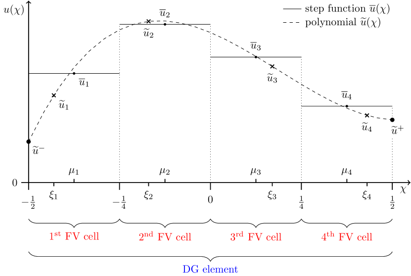
Figure 1: 1D schematic of four ($N=4$) mean values $\overline{\boldsymbol{u}}_{i}$ and their reconstructed nodal values (polynomial coefficients) $\widetilde{\boldsymbol{u}}_{i}$ constituting a polynomial of degree $3$ spanning over the whole DG element.

3.3.1 Projection & Reconstruction

In order to make FV and DG compatible, we define projection and reconstruction operators transforming between $N$ mean values $\overline{\boldsymbol{u}}_{i}$ and $N$ nodal values $\widetilde{\boldsymbol{u}}_{i}$. For the projection operator $\mathcal{P}\in\mathbb{R}^{N\times N}$, we make the following ansatz with $i=1,\dots,N$

$$\overline{\boldsymbol{u}}_{i}=N\int_{\mu_{i-\frac{1}{2}}}^{\mu_{i+\frac{1}{2}}}\widetilde{\boldsymbol{u}}(\chi)\,d\chi=\sum_{j=1}^{N}\widetilde{\boldsymbol{u}}_{j}\;\underbrace{N\,\int_{\mu_{i-\frac{1}{2}}}^{\mu_{i+\frac{1}{2}}}\ell_{j}(\chi)\,d\chi}_{:=\;\mathcal{P}_{ij}},$$ (42)

where the sub-cell centres, $\mu_{i}$, and interfaces, $\mu_{i\pm\frac{1}{2}}$, given as

$$\mu_{i}=-\frac{1}{2}+\frac{i}{N}-\frac{1}{2\,N}\quad\text{and}\quad\mu_{i\pm\frac{1}{2}}=\mu_{i}\pm\frac{1}{2\,N},$$ (43)

encode a regular sub-cell grid of $N$ finite volumes within the reference element $\big{[}-\frac{1}{2},\frac{1}{2}\big{]}$. By construction the projection matrix $\mathcal{P}$ is quadratic and non-singular. Hence, the inverse $\mathcal{R}:=\mathcal{P}^{-1}$ reconstructs $N$ nodal values from given $N$ mean values. We write

$$\overline{\boldsymbol{u}}_{ijk}=\sum_{c=1}^{N}\mathcal{P}_{kc}\sum_{b=1}^{N}\mathcal{P}_{jb}\sum_{a=1}^{N}\mathcal{P}_{ia}\>\>\widetilde{\boldsymbol{u}}_{abc}:=\mathcal{P}_{ijk}^{[abc]}\>\>\widetilde{\boldsymbol{u}}_{[abc]}\quad\text{and}\quad$$

$$\widetilde{\boldsymbol{u}}_{ijk}=\sum_{c=1}^{N}\mathcal{R}_{kc}\sum_{b=1}^{N}\mathcal{R}_{jb}\sum_{a=1}^{N}\mathcal{R}_{ia}\>\>\overline{\boldsymbol{u}}_{abc}:=\mathcal{R}_{ijk}^{[abc]}\>\>\overline{\boldsymbol{u}}_{[abc]},$$ (44)

where we introduce a variant of the Einstein notation for brevity. That is, indices enclosed in brackets are summed over.

3.3.2 Convex Blending

We aim to blend the right-hand-side solution of a LOW and HIGH order scheme with a continuous blending factor $\alpha\in[0,1]$ in a convex manner:

$$\partial_{t}\boldsymbol{u}_{q}\;=\;(1-\alpha)\,\partial_{t}\boldsymbol{u}_{q}^{\text{LOW}}\;+\;\alpha\,\partial_{t}\boldsymbol{u}_{q}^{\text{HIGH}}.$$

In order to make the disparate solution spaces for FV and DG compatible we transform the nodal values from DG to mean values and convex combine with the FV flux to the blended right-hand-side:

$$\partial_{t}\overline{\boldsymbol{u}}_{q,ijk}\;=\;(1-\alpha_{q})\,\partial_{t}\overline{\boldsymbol{u}}_{q,ijk}^{\text{FV}}\;+\;\alpha_{q}\,\mathcal{P}_{ijk}^{[abc]}\,\partial_{t}\widetilde{\boldsymbol{u}}_{q,[abc]}^{\text{DG}}.$$ (45)

We call $\alpha_{q}$ the volume blending factor, which can be chosen to be unique for each element. However, we have to carefully ensure the conservation property of the blending scheme by determining a common surface flux

$$\overline{\boldsymbol{F}}^{*}_{q\pm\frac{1}{2},jk}=(1-\alpha_{q\pm\frac{1}{2}})\,\overline{\boldsymbol{F}}^{*\text{FV}}_{q\pm\frac{1}{2},jk}+\alpha_{q\pm\frac{1}{2}}\,\mathcal{P}_{jk}^{[bc]}\,\widetilde{\boldsymbol{F}}^{*\text{DG}}_{q\pm\frac{1}{2},[cb]}.$$ (46)

We call $\alpha_{q\pm\frac{1}{2}}$ the surface blending factor, which is shared between neighbouring elements $q$ and $q~{}+~{}1$. The outermost fluxes in (3.1) are replaced with expression (46):

$$\overline{\boldsymbol{F}}^{*}_{q,1jk}\rightarrow\overline{\boldsymbol{F}}^{*}_{q-\frac{1}{2},jk}\quad\text{and}\quad\overline{\boldsymbol{F}}^{*}_{q,Njk}\rightarrow\overline{\boldsymbol{F}}^{*}_{q+\frac{1}{2},jk}.$$

Likewise, we replace the surface flux in (30) with the transformed flux (46):

$$\widetilde{\boldsymbol{F}}^{*}_{q\pm\frac{1}{2},jk}\rightarrow\mathcal{R}_{jk}^{[bc]}\,\overline{\boldsymbol{F}}^{*}_{q\pm\frac{1}{2},[bc]}.$$

The surface fluxes in y- and z-direction are computed analogously.

3.3.3 Calculation of the Blending Factor $\alpha$

The surface blending factors $\alpha_{q\pm\frac{1}{2}}$ are estimated from the relative differences in the jumps of the element mean values $\overline{\boldsymbol{u}}_{q,ijk}$ and the reconstructed polynomial $\widetilde{\boldsymbol{u}}_{q,ijk}$ at element interfaces $q\pm\frac{1}{2}$. As in the previous section, we transform the interpolated nodal interface values to mean values beforehand:

$$\overline{\kappa}^{\text{DG}}_{q\pm\frac{1}{2},jk}=\mathcal{P}^{[bc]}_{jk}\;\widetilde{\kappa}_{q\pm\frac{1}{2},[bc]},$$

where $\kappa$ is a freely chosen indicator variable, such as density or pressure. Additionally, we introduce the element interface jumps

$$\left[\left[\cdot\right]\right]_{q\pm\frac{1}{2},jk}=(\cdot)^{-}_{q\pm\frac{1}{2},jk}-(\cdot)^{+}_{q\pm\frac{1}{2},jk}$$ (47)

illustrated in Fig. 2. The blending factor in x-direction then reads

$$\alpha_{q\pm\frac{1}{2},jk}=1-\mathcal{T}\left(\left[\left[\overline{\kappa}^{\text{FV}}\right]\right]_{q\pm\frac{1}{2},jk},\left[\left[\overline{\kappa}^{\text{DG}}\right]\right]_{q\pm\frac{1}{2},jk}\right),$$ (48)

with the transfer function

$$\mathcal{T}\left((\cdot)^{\text{FV}},(\cdot)^{\text{DG}}\right)=\Bigg{\lfloor}_{0}\tau_{A}\,\frac{\left|\,(\cdot)^{\text{FV}}-(\cdot)^{\text{DG}}\right|-\tau_{S}\,\big{|}\,(\cdot)^{\text{FV}}\,\big{|}\,}{\max\big{(}\,\big{|}\,(\cdot)^{\text{FV}}\,\big{|},1\,\big{)}}\Bigg{\rceil}_{1},$$ (49)

mapping the two input arguments $(\cdot)^{\text{FV}},(\cdot)^{\text{DG}}\in\mathbb{R}$ to the unit interval $[0,1]$ as is indicated by the notation $\lceil_{0}\,(\cdot)\,\rceil_{1}$ trimming the input $(\cdot)$ for values below 0 and above 1. The amplification parameter, $\tau_{A}:=20$, and the shifting parameter, $\tau_{S}:=1.0$, are fixed for all numerical results shown in this work. Moreover, we choose the thermal pressure (5) as the indicator variable.

For the common surface blending factor we pick the minimum result along the interface:

$$\alpha_{q\pm\frac{1}{2}}=\min_{ij=1}^{N}\alpha_{q\pm\frac{1}{2},jk}.$$ (50)

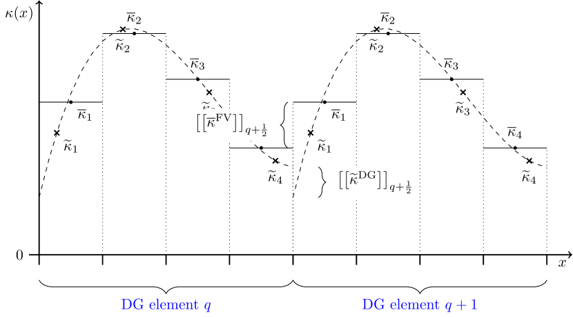
Figure 2: 1D schematic of two neighbouring elements $q$ and $q+1$ each with four ($N=4$) mean values of the indicator variable $\overline{\kappa}_{i}$ and their reconstructed polynomial coefficients $\widetilde{\kappa}_{i}$. The relative difference of the jumps at an element interface is considered to be a measure of the smoothness of the solution at hand.

For the volume blending factor $\alpha_{q}$ we calculate the averages of the surface blending factors in each direction, for example in x-direction

$$\alpha^{x}_{q}=\frac{1}{2}\big{(}\alpha^{x}_{q-\frac{1}{2}}+\alpha^{x}_{q+\frac{1}{2}}\big{)},$$

and determine the minimum among all directions

$$\alpha_{q}=\min\big{\{}\alpha^{x}_{q},\alpha^{y}_{q},\alpha^{z}_{q}\big{\}}.$$ (51)

The idea of the proposed algorithm is to have a mechanism which is designed such that for well resolved flows the solver yields the full DG solution and gradually shifts to the FV solution in case of discontinuities or strong under-resolution. Additionally, the blending factor is set to zero, if the reconstructed polynomial coefficients yield unbound values, such as negative densities or negative pressures. The result is then a 100% second-order slope limiting FV solution in elements where the reconstruction of a DG polynomial failed. Hence, in some sense, the proposed method with convex blending of a low and high-order operator guarantees that the discretisation cannot be "worse" than the second-order FV method.

3.4 Source terms

The discretisation of the gravity source term (18) is constructed in a straight forward manner by inserting the cell-averaged fluid state, i.e.

$$\overline{\boldsymbol{\Upsilon}}^{\text{gravity}}_{q,ijk}=\boldsymbol{\Upsilon}^{\text{gravity}}\big{(}\overline{\boldsymbol{u}}_{q,ijk}\big{)},$$

where the gravitational acceleration vector $\vec{g}$ in (18) comes in the form of mean values from the gravity modules provided by FLASH (e.g. the tree-based gravity solver by Wünsch et al., 2018). We do remark that this way of evaluating the source term, albeit very robust and straight forward to implement, is formally only second order accurate as the mean value of the sub-cell and not the DG polynomial evaluation is used. However, as already mentioned, the goal is to connect to the multi-physics framework as seamless as possible and this is one compromise taken.

3.5 Time Integration

Time integration of the semi-discrete equation (3.1) is done by explicit Runge-Kutta schemes, such as the optimal second order Ralston’s Method (Ralston, 1962) or the fourth order, five stages and strong-stability SSP-RK(5,4) variant (Spiteri & Ruuth, 2002).

To calculate a stable timestep the maximum eigenvalue estimate (11) is evaluated on all mean values $\overline{\boldsymbol{u}}_{q,ijk}$ in block $q$. In three dimensions it reads as

$$\overline{\lambda}_{q}^{\text{max}}=\max_{d=1}^{3}\max_{ijk=1}^{N}\lambda^{\text{max}}_{d}\Big{(}\overline{\boldsymbol{u}}_{q,ijk}\Big{)}.$$ (52)

Then the maximal timestep is estimated by the CFL condition

$$\Delta t:=\frac{CFL}{d}\,\min_{q}\;\frac{\min(\Delta x_{q},\Delta y_{q},\Delta z_{q})}{N\;\overline{\lambda}_{q}^{\text{max}}},$$ (53)

where $d=3,CFL:=0.4$ and $N$ is the number of mean values in each direction of the block $q$. Furthermore, we calculate the global hyperbolic correction speed (17) with

$$c_{h}=\max_{q}\,\max_{d=1}^{3}\max_{ijk=1}^{N}c_{d}\Big{(}\overline{\boldsymbol{u}}_{q,ijk}\Big{)}.$$ (54)

3.6 Enforcing Density and Pressure Positivity

In the conserved variables formulation (3), the thermal pressure (5) is derived from the total energy by subtracting the kinetic and magnetic energy terms. Hence, at strong shocks or under near-vacuum conditions the scheme can produce non-physical states. To alleviate this problem, we lift the troubled cells into positivity such that the permissibility condition

$$\big{\{}\text{permissible states}\big{\}}=\big{\{}\forall\,\boldsymbol{u}\;\big{|}\;\rho>0\wedge p(\boldsymbol{u})>0\big{\}}.$$ (55)

is fulfilled for all cells in a block $q$. First, we calculate the block average

$$\langle\boldsymbol{u}\rangle_{q}=\frac{1}{N^{3}}\sum_{ijk=1}^{N}\,\overline{\boldsymbol{u}}_{q,ijk}$$ (56)

and then determine a ’squeezing’ parameter $\beta\in[0,1]$ which enforces physical states:

$$\overline{\boldsymbol{u}}_{q,ijk}^{\text{physical}}=(1-\beta)\,\langle\boldsymbol{u}\rangle_{q}+\beta\;\overline{\boldsymbol{u}}_{q,ijk}\quad\in\big{\{}\text{permissible states}\big{\}}.$$ (57)

The algorithm to find a suitable $\beta$ is straightforward. One starts with $\beta:=1$ and decrements in steps of $\Delta\beta:=0.1$ till the permissibility condition is fulfilled. The advantage of this algorithm lies in its simplicity and it is conservative by construction. However, it fails when the block average is not part of the permissible set. In this case the code crashes and the simulation stops. For the results presented in this paper this worst case never happened.

4 Implementation in FLASH

The FLASH code is a modular, parallel multi-physics simulation code capable of handling general compressible flow problems found in many astrophysical environments. It uses the Message Passing Interface (MPI) library for inter-processor communication and the HDF5 or Parallel-NetCDF library for parallel I/O to achieve portability and scalability on a variety of different parallel computers. The framework provides three interchangeable grid modules: a Uniform Grid, a block-structured octree based adaptive grid using the PARAMESH library (Olson et al., 1999) and a block-structured patch based adaptive grid using Chombo (Colella et al., 2009). The architecture of the code is designed to be flexible and easily extensible.

The numerical scheme described in Section 3 has been implemented within FLASH as an independent solver module named DGFV under the hydro/HydroMain/split namespace. Although our numerical scheme is technically an unsplit solver it mimics the same interface as the other directionally split solvers since most physics modules necessary for our envisaged astrophysics simulations only interface to directionally split schemes. Contrary to the described 3D FV scheme in Section 3.1 we cannot split the 3D DGSEM scheme from Section 3.2 into separate arrays of 1D data; at least not without compromising the accuracy. These so called sweeps in spatial direction $d$ are treated independently by directionally split schemes and assembled to the new solution afterwards. Fortunately, the split scheme interface is flexible enough to accommodate a high-order (unsplit) DG scheme.

Figure 3: Cross section of a PARAMESH grid with blocks of $8^{3}$ cells at different refinement levels (i.e. mesh resolution). The block of interest is shaded in yellow and its guard cell layer is shaded in grey. One 4^th-order DG element with its adjacent elements is highlighted in blue and the blue dots indicate the position of the Gauss quadrature nodes (29). The red square with its red midpoint exemplifies one FV cell in the block.

We focus our solver implementation on the octree-based grid unit PARAMESH which is the default in FLASH. PARAMESH is built on the basic component of blocks consisting of $N_{x}\times N_{y}\times N_{z}$ regular cells extended with $N_{g}$ layers of guard cells. Fig. 3 shows a cross section of such a PARAMESH grid. The block of interest is coloured in yellow while the guard cells are shaded in grey. The complete computational grid consists of a collection of such blocks with different physical cell sizes. They are related to each other in a hierarchical fashion using a tree data structure (octree). Blocks do not overlap and there are only jumps of maximal one refinement level allowed between neighbours sharing a common face.

PARAMESH handles the filling of the guard cells with information from neighbouring blocks or at the boundaries of the physical domain. If the block’s neighbour has the same level of refinement, PARAMESH fills the corresponding guard cells using a direct copy from the neighbour’s interior cells. If the neighbour is at a higher refinement level, the data is restricted via second order averaging. If the neighbour is at a lower refinement level, the data is prolongated via monotonic interpolation guaranteeing positive densities and pressures.

The default configuration in FLASH is $N_{x}=N_{y}=N_{z}:=8$ and $N_{g}:=4$, which allows us to implement a fourth order DG method ($N=4$) with $2^{3}$ elements embedded within a block. In Fig. 3 one DG element and its DG neighbours are highlighted in blue. The blue dots represent the Legendre-Gauss quadrature nodes (29). The nodal state values of the DG element are reconstructed from the underlying mean values as described in Section 3.3.1.

What follows is a brief outline of the algorithm implemented within the DGFV solver module. The module enters the Runge-Kutta cycle of $m$ stages starting with the first stage. A full timestep is completed after exiting the loop with the last stage where we compute the global timestep of the next cycle according to the CFL condition (53). The updated states are returned back to FLASH, which in turn calls the other modules handling different aspects of the simulation such as grid coarsening/refinement, load balancing, gravity, chemistry, etc. At the beginning of each Runge-Kutta stage the guard cells of each block are filled by PARAMESH with the latest data from direct neighbours. We reconstruct the nodal data of the DG elements via (3.3.1) and compute the blending factors according to Section 3.3.3. If any of the calculated blending factors is less than one, indicating under-resolved flow features within a DG element, the blending procedures are activated and we compute the standard FV solution described in Section 3.1. Otherwise it suffices to just compute the DG solution from the reconstructed nodal values according to Section 3.2. If blending is active one has to determine the common surface fluxes (46) at DG element interfaces in order to maintain the conservation property. The final solution is then the convex blend (45) of both solutions. Moreover, the (common) surface fluxes at block boundaries are handed over to PARAMESH, which does a flux correction by replacing the coarse fluxes with the restricted fine fluxes at non-conforming block interfaces. We retrieve the corrected fluxes and calculate the total surface flux error among all block boundaries. The error is then evenly deducted from all cells restoring mass conservation. Finally, we calculate the gravity source terms (18), which we add to the solution. The solver can now proceed to the next Runge-Kutta stage. This completes the outline of the algorithm.

Three remarks are in order. Firstly, FLASH stores its fluid data in primitive state variables. For DG we need to reconstruct on conservative state variables in order to maintain high-order accuracy and stability. In other words, the conservative state variables are first calculated from the primitive state variables in mean value space and then transformed to nodal values. Secondly, the treatment at non-conforming block interfaces by PARAMESH is at most second order accurate. For DG the standard approach is the so called mortar method (Kopriva et al., 2002), which matches the spatial order of the scheme if done correctly. However, we decided to stick with the default procedure provided by PARAMESH since it would otherwise lead to substantial restructuring of the internal workings of the FLASH code. Furthermore, we observed that in practice the gain in accuracy by a higher-order mortar method is negligible in our simulations, neither do we have any troubles with numerical artefacts or stability issues. Thirdly, physics and chemistry units in FLASH are designed and implemented around mean values, i.e. they expect mean values as input, do their calculations on mean values and produce mean values as output. As mentioned already in Section 3.4 about source terms, this formally reduces the convergence order to at most second order, however, provides the benefit of directly using the rich collection of physics modules available in the FLASH framework.

5 Numerical Results

In this section, we present simulation results using our new 4^th-order (DGFV4) fluid solver module in FLASH. All test problems shown are computed on 1D, 2D or 3D Cartesian grids, for which the refinement level $l$ corresponds to $2^{l-1}\times 8$ grid points per dimension. We gradually increase the complexity of the test cases, where the later test cases are multi-physics applications with multiple physics modules working together.

5.1 Experimental Order of Convergence

First, we verify the experimental order of convergence (EOC) of our 4^th-order DGFV4 implementation. Measuring convergence of higher-order MHD codes can be challenging since smooth MHD test problems present numerical subtleties that are potentially revealed by the very low numerical dissipation of higher-order methods. In this work, we rely on common, smooth MHD test problems for convergence assessment: the non-linear circularly polarised Alfvén waves in 2D and a manufactured solution setup for 3D.

For our convergence tests, we enable any shock indicators and limiters on purpose in order to confirm that the limiters do not interfere for smooth and well resolved solutions.

To study the convergence properties of the code, we compute the numerical errors, that is, the norm of the difference of the numerical solution, $u_{\text{num}}$, from the reference solution, $u_{\text{ref}}$, with mean values. In this work, we look at the $\infty$-norm, i.e.

$$\big{|}\big{|}\overline{u}_{\text{num}}-\overline{u}_{\text{ref}}\big{|}\big{|}_{\infty}=\max_{q=1}^{Q}\max_{ijk=1}^{N}\Big{|}\overline{u}_{\text{num},q,ijk}-\overline{u}_{\text{ref},q,ijk}\Big{|}$$ (58)

and the 2-norm, i.e.

$$\big{|}\big{|}\overline{u}_{\text{num}}-\overline{u}_{\text{ref}}\big{|}\big{|}_{2}=\left[|\Omega|^{-1}\sum_{q=1}^{Q}\sum_{ijk=1}^{N}\frac{V_{q}}{N^{3}}\Big{|}\overline{u}_{\text{num},q,ijk}-\overline{u}_{\text{ref},q,ijk}\Big{|}^{2}\right]^{\frac{1}{2}},$$ (59)

where $V_{q}=\Delta x_{q}\,\Delta y_{q}\,\Delta z_{q}$ is the volume of block $q$ and $|\Omega|$ is the volume of the computational domain.

We note that one has to compute the mean values of the reference solution with high accuracy as they should formally be the exact mean values of the reference solution. Hence, we evaluate the reference solution on quadrature nodes of the same order or higher as in (34) and then project to mean values.

Circularly polarised smooth Alfvén waves are exact analytic solutions of the MHD equations for arbitrary wave amplitude perturbations. Hence, they are suitable to study the experimental convergence order of the scheme, as well as its amount of numerical dispersion and dissipation errors. The solution consists of plane waves in which the magnetic field and velocity oscillate in phase in a circular polarisation perpendicular to the propagation direction.

We initialise the Alfvén waves within a periodic 2D domain $\Omega=[0,0]\times[\cos^{-1}(\alpha),\sin^{-1}(\alpha)]$ at an angle of $\alpha=45^{\circ}$. The longitudinal Alfvén wave speed is fixed at $|v_{A}|=B_{||}/\sqrt{\rho}:=1$, such that the wave returns to its initial state at integer times $T\in\mathbb{N}$. For our test we let the wave turn around five times, i.e. $T=5$. The heat capacity ratio is $\gamma=5/3$. With the rotated coordinate $\hat{x}=x\,\cos(\alpha)+y\,\sin(\alpha)$, we define $B_{\perp}=0.1\,\sin(2\pi\,\hat{x})$ and $B_{3}=0.1\,\cos(2\pi\,\hat{x})$. The initial state in primitive state variables then reads $(\rho,\vec{v},p,\vec{B},\Psi)^{T}=(1.0,\vec{v}_{0},0.1,\vec{B}_{0},0)^{T}$ with $\vec{v}_{0}=(-B_{\perp}\sin(\alpha),B_{\perp}\cos(\alpha),B_{3})^{T}$ and $\vec{B}_{0}=(\cos(\alpha),\sin(\alpha),0)^{T}+\vec{v}_{0}$. We look at the total pressure (2) and calculate the $\infty$-norm and 2-norm according to (58) and (59). Since the total pressure involves all state variables it is a good quantity to measure the overall convergence of the code. The results are shown in Table 1. The formally 4^th-order DGFV4 scheme in 2D yields the expected EOCs.

Table 1: EOC of total pressure $P$ of the smooth Alfvén wave problem in 2D run by the 4^th-order DGFV4 scheme.

cells	$\big{|}\big{|}P\big{|}\big{|}_{\infty}$	$\big{|}\big{|}P\big{|}\big{|}_{2}$	EOC∞	EOC2
$16^{2}$	9.852e-05	4.951e-05	n/a	n/a
$32^{2}$	6.086e-06	2.110e-06	4.016	4.552
$64^{2}$	3.634e-07	1.285e-07	4.065	4.036
$128^{2}$	2.334e-08	8.002e-09	3.960	4.006
$256^{2}$	1.461e-09	4.998e-10	3.997	4.000
$512^{2}$	9.221e-11	3.423e-11	3.985	3.868

Next, in order to verify the convergence order in 3D we construct a manufactured solution which, in primitive state variables, reads as

$$\boldsymbol{\Phi}^{\text{man}}=\big{(}h,0.1,0.2,0.3,h,h,-h,1,0\big{)}^{T}$$ (60)

with $h=h(t,x,y,z)=0.5\sin(2\pi(x+y+z-t))$. The domain is a cubic box $\Omega=[0,1]^{3}$ and the heat capacity ratio is set to $\gamma=2.0$. At each Runge-Kutta stage we subtract the residual

$$\boldsymbol{\Upsilon}^{\text{man}}=\partial_{x}F\big{|}_{\boldsymbol{\Phi}^{\text{man}}}+\partial_{y}G\big{|}_{\boldsymbol{\Phi}^{\text{man}}}+\partial_{z}H\big{|}_{\boldsymbol{\Phi}^{\text{man}}}$$ (61)

from the numerical solution $\partial_{t}\boldsymbol{u}$ and advance in time. As before, the source term is evaluated with an appropriate quadrature rule and projected to mean values. At final time $T=0.1$ the convergence of the total pressure (2) is computed as previously described in the Alfvén wave test. The results in Table 2 confirm the correct EOCs for the formally 4^th-order DGFV4 scheme in 3D.

Table 2: EOC of total pressure $P$ of the manufactured solution problem in 3D run by the 4^th-order DGFV4 scheme.

cells	$\big{|}\big{|}P\big{|}\big{|}_{\infty}$	$\big{|}\big{|}P\big{|}\big{|}_{2}$	EOC∞	EOC2
$16^{3}$	1.259e-03	4.122e-04	n/a	n/a
$32^{3}$	4.998e-05	1.773e-05	4.655	4.538
$64^{3}$	3.248e-06	1.015e-06	3.943	4.126
$128^{3}$	1.962e-07	6.594e-08	4.048	3.944
$256^{3}$	1.290e-08	4.141e-09	3.927	3.992
$512^{3}$	7.963e-10	2.540e-10	4.018	4.027

5.2 Divergence Control

We now turn to test problems more specifically aimed at evaluating the efficacy of the hyperbolic divergence cleaning scheme discussed in Section 2.1.4.

5.2.1 Magnetic Loop Advection

This test investigates the proper advection of a magnetic field loop (Gardiner & Stone, 2005). On a periodic domain $\Omega=[-0.5,0.5]^{2}$, the background medium has $\rho=1$, $p=1$, and a global advection velocity $(v_{1}v_{2})=(2,1)$ so that the ambient flow is not aligned with any coordinate axis. Letting $r=\sqrt{x^{2}+y^{2}}$ be the radial distance to the centre of the domain, the magnetic field is initialised from a vector potential $\vec{A}=(0,0,A_{3}(r))$ with $\vec{B}=\nabla\times\vec{A}$. To define a magnetic field loop of radius $r_{0}=0.3$, we set $A_{3}(r)=\max(0,10^{-3}(r_{0}-r))$ and obtain a very weakly magnetised configuration with a plasma $\beta$ of order $10^{6}$, in which the magnetic field is essentially a passive scalar. For this field configuration, the MHD current vanishes everywhere, except at $r=0$, and $r=r_{0}$ where the corresponding current line and current tube become singular. Note, that we added a smoothing parameter $\delta r=0.05$ to $r$ in order to avoid spurious ringing caused by the unresolved singularity of the initial magnetic field at the domain centre. The aim of the test is to verify that the current loop is advected without deformation or noise.

Fig. 4 shows the z-component of the current density $\vec{j}=\nabla\times\vec{B}$ at final time $T=1$ corresponding to two horizontal domain crossings. The test is carried out with a uniform resolution of $128^{2}$ cells. The current density is a stringent diagnostic since, being a derivative of the magnetic field, it is very sensitive to noise and local fluctuations. The scheme preserves the exact circular shape of the current loop very well, with very little noise and oscillations in the current.

Figure 4: We show the $z$-component of the current density $\vec{j}=\nabla\times\vec{B}$ for the final time $T=1.0$ as calculated with the DGFV4 scheme.

5.2.2 MHD Current Sheet

The two-dimensional current sheet problem in ideal MHD regimes has been extensively studied before (see e.g. Gardiner & Stone, 2005; Guillet et al., 2019; Rastätter et al., 1994; Rueda-Ramírez et al., 2021). Two magnetic currents are initialized in opposite direction sharing a common interface and disturbed with a small velocity fluctuation which provokes magnetic reconnections. In the regions where the magnetic reconnection takes place, the magnetic flux approaches very small values and the lost magnetic energy is converted into internal energy. This phenomenon changes the overall topology of the magnetic fields and consequently affects the global magnetic configuration.

The square computational domain is given as $\Omega=[-0.5,0.5]^{2}$ with periodic boundary conditions. We initialise the setup in primitive variables $(\rho,\vec{v},p,\vec{B},\Psi)^{T}=(1.0,v_{1},0,0,0.05\,B_{0}^{2},0,B_{2}.0,0)^{T}$ with $B_{0}=1/\sqrt{4\pi}$, $v_{1}=0.1\sin(2\pi y)$ and $B_{2}=-B_{0}$ when $-0.25<x<0.25$ and $B_{2}=B_{0}$ in the rest of the domain. The heat capacity ratio is set to $\gamma=5/3$ and the final simulation time is $T=10$. The simulation is carried out with a uniform resolution of $256^{2}$ cells.

The changes in the magnetic field seed the magnetic reconnection and develop formations of magnetic islands along the two current sheets. The small islands are then merged into bigger islands by continuously shifting up and down along the current sheets until there is one big island left in each current sheet. The final result is shown in Fig. 5, which depicts the $z$-component of the current density with overlayed magnetic field lines.

Figure 5: We show the $z$-component of the current density $\vec{j}=\nabla\times\vec{B}$ with overlayed magnetic field lines for the MHD current sheet test at final time $T=10$.

Fig. 6 shows the domain-integrated divergence error over time for three different runs: without any divergence cleaning (none; blue line), with just Powell source terms (Powell; orange line) and with Powell source terms plus hyperbolic divergence cleaning (Powell + hyb. div. cleaning; green line) which is the default in our code. The first simulation crashes early on due to the rapid surge of divergence error leading to the well known instability issues of uncontrolled magnetic field divergence growth in MHD simulations (Brackbill & Barnes, 1980; Tóth, 2000; Kemm, 2013). The second run with Powell terms does not crash and is at least able to keep the overall errors at bay over the course of the simulation (see also Fig. 7). As expected, the run with hyperbolic divergence cleaning has the lowest divergence error at all times. This particular setup is insofar challenging in that it perpetually prompts a significant production of divergence errors, thus highlighting the importance of a proper and robust divergence cleaning technique.

Figure 6: Evolution of the domain-integrated absolute magnetic field divergence $\int_{\Omega}|\nabla\cdot\vec{B}(t)|d\Omega$ for the MHD current sheet test. Three runs with different flavours of divergence cleaning are shown. The simulation without any divergence correction method ("none"; blue line) crashed at around $t=2.5$. The run where only the Powell source terms are used (orange line) is stable but has a substantially larger divergence error than the full scheme with Powell source terms and hyperbolic divergence cleaning (green line) which is the default setting in our code.

Fig. 7 shows the time evolution of the kinetic, internal, magnetic, and total energies of the current sheet problem with (solid lines) and without (dashed lines) hyperbolic divergence cleaning activated (see Section 2.1.4). The decline of the magnetic energy is compensated by the increase in internal energy due to the heating driven by the magnetic reconnection. Furthermore, without divergence cleaning a significant total energy drift is introduced by the non-conservative Powell terms and the accompanied high divergence errors, which are not properly corrected for in this case. This energy drift also causes artificial cooling at the reconnection points giving rise to a non-physical behaviour. However, with hyperbolic divergence cleaning the total energy is conserved.

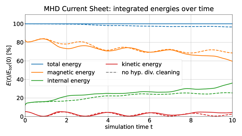
Figure 7: The percentage of total and individual energies as a function of time for the MHD current sheet test. We compare the results with (solid lines) and without (dashed lines) our hyperbolic divergence cleaning method. The results for the run without any divergence treatment is not shown since it crashed early on.

5.3 Shock Problems

In this section, we test the correct resolution of shock waves inherent to ideal MHD regimes by our DGFV4 scheme in 1D, 2D and 3D. Furthermore, one shock tube problem investigates the proper handling of waves in a multi-species setting and we also utilise adaptive mesh refinement for a further challenge. Note that we actually run all our 1D test problems in 2D, with perfectly $y$-independent initial conditions and periodic boundaries. A correct implementation of our multidimensional scheme does not develop any $y$-dependence of the solution.

5.3.1 Briu-Wu Shock Tube

The established MHD shock tube problem introduced by Brio & Wu (1988) has now become a classic shock test for MHD codes. For this test, we take the computational domain to be $[0,1]$ with outflow boundaries left and right. In the whole domain, the flow is initially at rest ($v=0$) and $(B_{1},B_{2})=(0.75,0)$. The initial primitive variables are discontinuous at $x=0.5$, with the left and right states given by $(\rho,p,B_{2})_{\mathrm{L}}=(1,1,1)$ and $(\rho,p,B_{2})_{\mathrm{R}}=(0.125,0.1,-1)$, respectively. We set $\gamma=2$, and run the simulation until the final time $T=0.1$.

Fig. 8 presents the density, pressure, and $y$-component of the magnetic field of the Brio-Wu shock tube test problem at final time $T=0.1$, using the DGFV4 scheme on an AMR grid with a minimum resolution of 32 cells and a maximum resolution of 512 cells. The reference solution is obtained using the latest version of ATHENA (v4.2) (Stone et al., 2008) with default settings on 2048 cells. Our DGFV4 scheme captures all the MHD waves correctly, and the limiter sharply resolves the shocks and the contact discontinuity within very few cells. The limiter sufficiently suppresses overshoots and oscillations around shocks. Furthermore, our scheme cooperates well with the standard AMR method provided by FLASH (not directly visible in Fig. 8) and properly traces the shock fronts at the highest resolution possible.

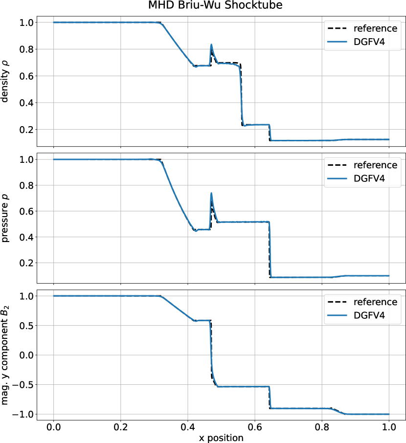
Figure 8: Density, pressure and magnetic field profiles of the Briu-Wu shock tube at final time $T=0.1$ run by the DGFV4 scheme on an AMR grid with a minimum resolution of 32 cells and a maximum resolution of 512 cells. We compute the reference solution with the ATHENA code using a resolution of 2048 cells.

5.3.2 MHD Shu-Osher Shock Tube

The MHD version of the 1D Shu-Osher shock tube test (Shu & Osher, 1988) proposed by Susanto (2014) becomes increasingly popular (Derigs et al., 2016; Guillet et al., 2019) to test the scheme’s ability to resolve small-scale flow features in the presence of strong shocks in ideal MHD regimes.

The setup follows the interaction of a supersonic shock wave with smooth density perturbations. The computational domain is $\Omega=[-5,5]$ with outflow boundary conditions. At $t=0$, the shock interface is located at $x_{0}=-4$. In the region $x\leq x_{0}$, a smooth supersonic flow is initialised with primitive states given by $(\rho,\vec{v},p,\vec{B},\Psi)=(3.5,5.8846,1.1198,0,42.0267,1,3.6359,0,0)$. In the rest of the domain $x>x_{0}$, smooth stationary density perturbations are setup in primitive state as $(1+0.2\sin(5\,x),0,0,0,1,1,1,0,0)$. The flow is evolved until the final time $T=0.7$.

The resulting density profile at the final time $T$ is shown in Fig. 9, for two maximum resolution levels: 256 cells and 512 cells. As in the Briu-Wu shock tube, we employ AMR in order to confirm the correct tracking of the small-scale flow features and the smooth interplay with our MHD solver. The reference solution has been computed using ATHENA on 2048 grid cells. Our scheme properly resolves all expected flow features for both levels of resolutions shown.

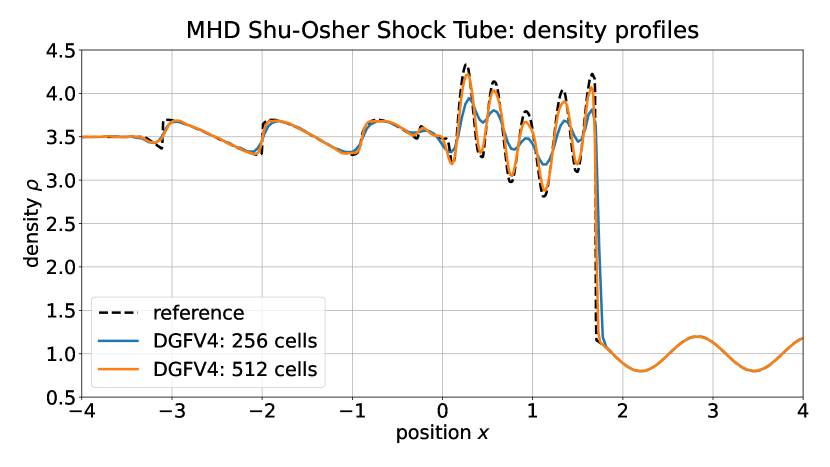
Figure 9: MHD Shu-Osher shock tube test problem: The density profile is shown at final time $T=0.7$. The reference solution has been computed using ATHENA on 2048 grid cells.

5.3.3 Two-component Sod Shock Tube

We simulate a Sod shock tube problem extended with two species as done for example in Gouasmi et al. (2020). The computational domain is $\Omega=[0,1]$ with outflow boundary conditions. At $t=0$, the shock interface is located at $x_{0}=0.5$. In the region $x\leq x_{0}$, the fluid is initialised with primitive states given by $(\rho,v,p,\sigma_{1},\sigma_{2})=(1,0,1,1,0)$. In the rest of the domain $x>x_{0}$, we setup the primitive states $(\rho,v,p,\sigma_{1},\sigma_{2})=(0.125,0,0.1,0,1)$. The individual heat capacity ratios of the two fluid components are $\gamma_{1}=1.4$ and $\gamma_{2}=1.6$ with equal heat capacities for constant volume $c^{\text{vol.}}_{1}=c^{\text{vol.}}_{2}=1$. The shock tube is evolved until the final time $T=0.2$ run by the DGFV4 scheme on an AMR grid with a minimum resolution of 32 cells and a maximum resolution of 256 cells. Fig. 10 shows the total density, pressure and specific heat ratio profiles at the final time. There is an excellent agreement with the exact solution provided by Karni (1994).

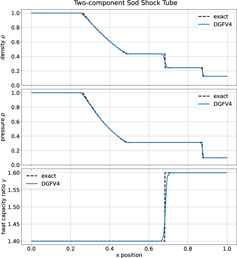
Figure 10: Two-component Sod shock tube problem: The profiles of the numerical solution with the DGFV4 scheme (on an AMR grid with a minimum resolution of 32 cells and a maximum resolution of 256 cells) together with the exact solution are shown at final time $T=0.2$.

5.3.4 Orszag–Tang Vortex

Now we look at the 2D Orszag–Tang vortex problem (Orszag & Tang, 1979), a widely-used test problem for ideal MHD. The vortex starts from a smooth initial field configuration, and quickly forms shocks before transitioning into turbulent flow. For this problem, our computational domain is $\Omega=[0,1]^{2}$ and we use $\gamma=5/3$. The initial density and pressure are uniform, $\rho=1$ and $p=1/\gamma$. The initial fluid velocity is $\vec{v}=(-\sin(2\pi\,y),\sin(2\pi\,x),0)^{T}$, and the initial magnetic field is $\vec{B}=(-\sin(2\pi\,y),\sin(4\pi\,x),0)^{T}/\gamma$.

The final solution at time $T=0.5$ is shown in Fig. 11. We employ an AMR grid with resolution levels going from $64^{2}$ cells to $1024^{2}$ cells, which is highlighted as black lines on the left half of the density plot. We recognise the well-known density distribution of the Orszag–Tang vortex, which is commonly presented in MHD code papers. Note that we obtain both sharp shocks and smooth, noise-free flow with resolved features between the shocks.

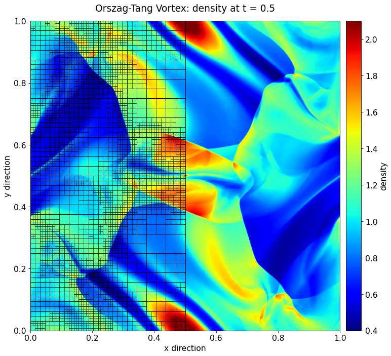
Figure 11: Density profile of the Orszag-Tang vortex at the final time $T=0.5$ as calculated with our DGFV4 scheme on an AMR mesh (shown as black lines in the left half of the plot) with a maximum refinement level of $l=8$, which is equivalent to a maximum resolution of $1024^{2}$ cells.

In order to corroborate the correct positioning of the shock waves, we computed a reference solution on a finer grid of $2048^{2}$ cells with the ATHENA code and overlay 1D cuts of both pressure solutions in Fig. 12. The resulting profile of our scheme matches the reference very well and is very sharp and without spurious oscillations or overshoots.

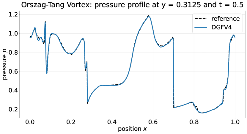
Figure 12: Numerical solution of the pressure profiles at $y=0.3125$ and time $T=0.5$ are shown for the DGFV4 solver with AMR and a maximum resolution of $1024^{2}$ cells. The reference solution has been computed with the ATHENA code at a uniform resolution of $2048^{2}$ cells.

During our numerical experiments we found that without proper divergence cleaning, distinctive grid artefacts appear, which considerably pollute the solution. Analog to Section 5.2.2 we compared the time evolution of the divergence errors with and without divergence control mechanisms. The results shown in Fig. 13 clearly demonstrate that the hyperbolic divergence cleaning method is effective in confining the divergence errors ensuring a clean, unpolluted MHD flow.

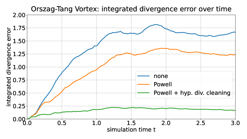
Figure 13: Domain-integrated divergence error $\int_{\Omega}|\nabla\cdot\vec{B}|d\Omega$ as a function of the simulation time for the Orszag-Tang vortex setup. Three runs with the DGFV4 are shown where the Powell scheme and hyperbolic divergence cleaning are either on or off. The simulation without any divergence correction method activated is labelled as "none".

5.3.5 Magnetic Rotor

We now investigate the 2D MHD rotor problem introduced by Balsara & Spicer (1999). In this setup, a dense disc of fluid rotates within a static fluid background, with a gradually declining velocity layer between the disk edge and the ambient fluid. An initially uniform magnetic field is present, winding up with the disc rotation and containing the dense rotating region through magnetic field tension. The computational domain is set to $\Omega=[0,1]^{2}$. Initial pressure and magnetic fields are uniform in the whole domain, with $p=1$ and $\vec{B}=(5/4\pi,0,0)^{T}$. The central, rotating disc is defined by $r<r_{0}$ where $r^{2}=(x-0.5)^{2}+(y-0.5)^{2}$, and $r_{0}=0.1$. Inside the disc, $\rho=10$, and the disc rotates rigidly with $\vec{v}=(0.5-y,x-0.5)v_{0}/r_{0}$ with $v_{0}=2$. The background fluid has a density of $\rho=1$ and is at rest: $\vec{v}=\vec{0}$. In the annulus $r_{0}\leq r\leq r_{1}=0.115$, the transition region linearly interpolates between the disc and the background, with $\vec{v}=(0.5-y,x-0.5)v_{0}f/r_{0}$ and $\rho=1+9f$, where $f=(r_{1}-r)/(r_{1}-r_{0})$ is the transition function. The simulation runs until the final time $T=0.15$. We use outflow boundary conditions.

We present the density contours at $T=0.15$ in Fig. 14. The black lines in the left half the plot highlight the AMR grid bounded between refinement levels of $64^{2}$ cells to $1024^{2}$ cells. The contours of the evolved disc show a sharp and noise-free picture of the circular rotation pattern, which is in general a challenge for MHD codes.

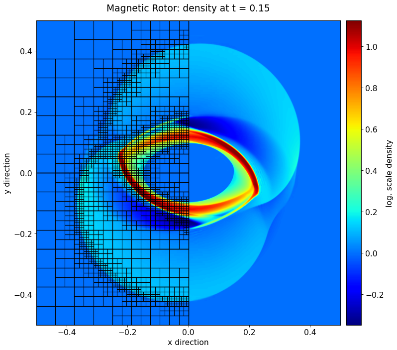
Figure 14: Density contours in logarithmic scale of the magnetic rotor at final time $T=0.15$ calculated with DGFV4 on an dynamic AMR mesh (shown as black lines in the left half of the plane) with a maximum refinement level of $l=8$ which is equivalent to a maximum resolution of $1024^{2}$ cells.

In Fig. 15, we plot the local magnetic field divergence error $|\nabla\cdot\vec{B}|$ of the DGFV4 solver at the final simulation time. The error is mostly concentrated in regions around shocks and radially propagates away in all directions (circular ripples) due to the hyperbolic divergence advection mechanism detailed in Section 2.1.4. Preferably, the divergence error gets advected out of the domain but, as clearly visible in the divergence plot, the errors can accumulate in stagnant regions of the domain, which justifies the importance of the damping source term (16) as an additional mechanism to dispose of any accrued magnetic field divergence errors.

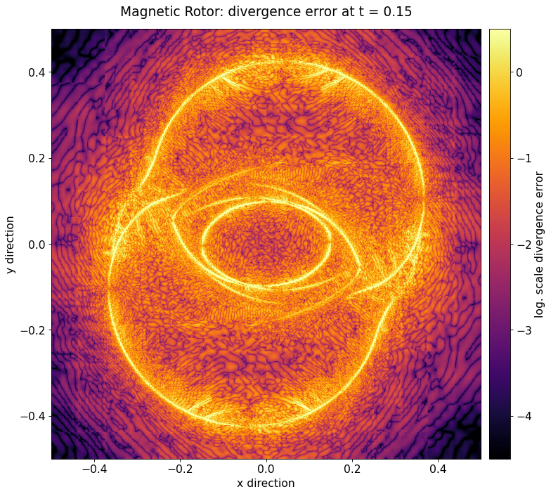
Figure 15: Contours of the local divergence error $|\nabla\cdot\vec{B}|$ in logarithmic scale of the magnetic rotor run by the DGFV4 scheme at final time $T=0.15$.

5.3.6 MHD Blast

In order to test the shock-capturing performance of our code for a very strong ideal MHD shock problem in 3D, we utilise the 3D blast wave setup of Balsara et al. (2009). The computational domain is set to $\Omega=[0,1]^{3}$ with outflow boundary conditions. The background fluid is initially at rest with respect to the grid, where $\vec{v}=\vec{0}$, $\rho=1$, and with a uniform magnetic field $\vec{B}=(100\sqrt{3},100\sqrt{3},0)$. The ambient pressure is set to $p=10^{-1}$, and within a central sphere of radius $r_{0}=0.1$, we set $p=10^{3}$ to initialise the blast. This creates an extreme initial shock strength with a pressure ratio of $10^{4}$ in a strongly magnetised background with a plasma-$\beta$ of $\approx 10^{-5}$ . We take $\gamma=1.4$, and run the simulation until the final simulation time $T=0.01$. The AMR grid is bounded between refinement levels of $64^{3}$ cells to $256^{3}$ cells.

In Fig. 16, we show a slice at $z=0$ of the magnetic pressure at the final time. The black lines in the left half of the plot highlight the AMR grid, while the light grey arrows trace the magnetic field lines of the solution. The originally spherical blast bubble gets stretched along the magnet background field over the course of the simulation as is described by Balsara et al. (2009). Our scheme is able to maintain positivity of the pressure and density in the whole domain and correctly captures the very strong discontinuities, while resolving the complex structures within the blast shell. Note that no oscillations are visible around discontinuities. This test shows the robustness and shock-capturing performance of our blending scheme for three-dimensional problems involving very strong magnetised shocks.

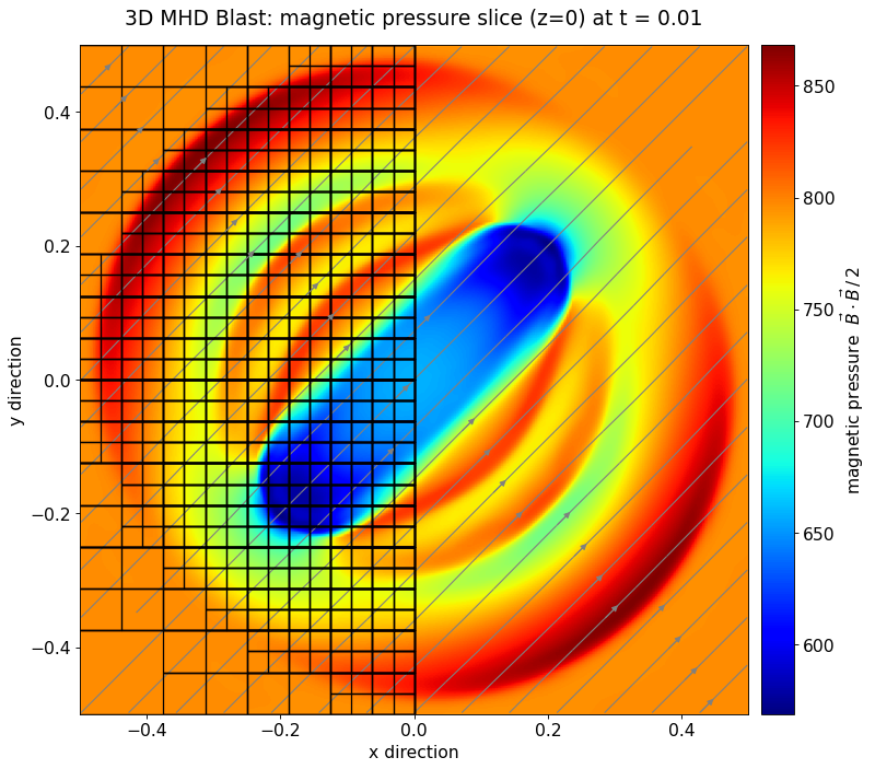
Figure 16: Slice of the magnetic pressure at $z=0$ for the MHD blast wave test solved with the DGFV4 scheme. The black lines on the left side highlight part of the AMR mesh and the grey stream lines indicate the field spanned by the $x$- and $y$-component of the magnetic field.

5.4 Coupling to Gravity

The FLASH framework provides specialised units for the employment of static gravitational sources emanating from point masses distributed at arbitrary points within the computational domain or from external background fields. Furthermore, FLASH unites a variety of solvers for the Poisson equations of gravity for mass distributions (self-gravity) based on multi-pole expansions (Müller & Steinmetz, 1995), tree-based Barnes-Hut algorithms (BHTree) (Barnes & Hut, 1986; Wünsch et al., 2018), multi-grid methods (Ricker, 2008) or hybridized schemes (Pfft) (Daley et al., 2012).

At first, we show an interesting MHD simulation using the static point mass module in FLASH and in the second part we verify the proper coupling of our code to the gravity solvers in FLASH for the case of the tree solver implementation by Wünsch et al. (2018).

5.4.1 Differentially Rotating MHD Torus

Here, we present the results of a three-dimensional global MHD simulation of magneto-rotationally instabilities (MRI) growing in a differentially rotating torus initially threaded by a toroidal magnetic field (Okada et al., 1989). After several rotation periods the inner region of the torus becomes turbulent due to the growth of the MRI fuelling efficient angular momentum transport processes (Velikhov, 1959; Chandrasekhar, 1960; Balbus & Hawley, 1990). Magnetic loops emerge by the buoyant rise of magnetic flux sheets from the interior of the torus (Machida et al., 1999), also known as Parker instability (Parker, 1966). Owing to this angular momentum redistribution, the torus becomes flattened to a disc where interstellar material gradually accretes to the massive source of gravity at the centre. Consequently, this process leads to various interesting phenomena such as X-ray flares and jet formation.

Such setups are usually modelled with the ideal MHD equations in cylindrical coordinates $(r,\phi,z)$, but in this work we resort to the Cartesian coordinate system $(x,y,z)$. Following Machida et al. (1999), we adopt an equilibrium model of the magnetised torus in order to initialise the setup. The scales of the model are completely determined by the following parameters: gravitational constant $G$, mass of the central object $M$, initial angular momentum of the torus $L$, median radius of the torus $r_{0}$, characteristic density of the torus $\rho_{0}$, magnetic field strength of the initial toroidal magnetic field $B_{\phi}$ and the initial ratio of gas pressure to magnetic pressure $\beta_{0}$. For convenience we set all aforementioned parameters to unity: $G=M=L=r_{0}=\rho_{0}=B_{\phi}=\beta_{0}=1$. We assume the polytropic equation of state $p=K\,\rho^{\gamma}$ with constant $K=0.05$ and $\gamma=5/3$. The inviscid, non-resistive torus is embedded in non-rotating, non-self-gravitating ambient gas ($\rho=10^{-5}$) and evolves adiabatically. Radiative cooling effects are neglected. For the static gravitational field caused by the central mass, we use the Newtonian potential provided by the PointMass module. The Alfvén wave speed is calculated according to Okada et al. (1989) as

$$c_{\text{Alfv\'{e}n}}^{2}=\frac{2\,K}{\beta_{0}}\big{(}\rho\,r^{2}\big{)}^{\gamma-1}\;\;\text{with}\;r^{2}=x^{2}+y^{2},$$ (62)

and the sound speed $c_{\text{sound}}$ is defined by (10). We transform the equation of motion (Machida et al., 1999) to the potential form

$$\psi_{\text{torus}}=\text{const.}=-\frac{G\,M}{r}+\frac{L^{2}}{2\,r^{2}}+\frac{c_{\text{sound}}^{2}}{\gamma-1}+\frac{\gamma\,c_{\text{Alfv\'{e}n}}^{2}}{2\,(\gamma-1)}\;\Bigg{|}_{r\,=\,r_{0}}$$ (63)

and obtain an expression for the density distribution of the initial torus

$$\rho_{\text{torus}}=\left[\frac{\max\big{(}0,\psi_{\text{torus}}+G\,M/R-L^{2}/(2\,r^{2})\big{)}}{K\,\gamma/(\gamma-1)\big{(}1+r^{2\,(\gamma-1)}/\beta_{0}\big{)}}\right]^{1/(\gamma-1)}.$$ (64)

The torus rotates differentially according to the Keplerian velocity $v_{\phi}=\sqrt{G\,M/r}$. The computational domain is set to $\Omega=[-7,7]^{3}$ with outflow boundary conditions at all faces. The AMR grid is bounded between refinement levels of $64^{3}$ cells to $256^{3}$ cells. The first row in Fig. 17 shows what the initial torus looks like in our setup.

After several periods, regions of dominating magnetic pressure $(\beta<1)$ emerge, where magnetic flux buoyantly escapes from the disk leading to violent flaring activities. The loop-like structures, similar to those in the solar corona, are also visible in our simulation after eight rotation periods as shown in Fig. 17 in the second and third row. This setup shows that the DGFV4 solver is capable of simulating complex MHD flow configurations under the influence of a static gravitational potential, giving rise to magnetically driven structures over several spatial scales.

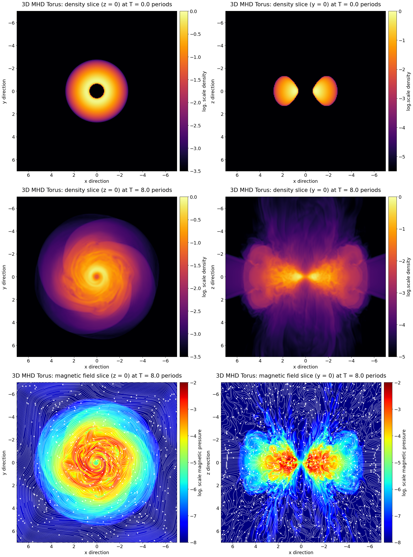
Figure 17: MHD torus at the initial time (top row) and after 8 periods: density (middle row) and magnetic field (bottom row) slices.

We further compare our implementation with another established MHD solver readily available in FLASH and perform simulations with different resolutions. The results can be found in appendix A.

5.4.2 Evrard Test

The Evrard test described by Evrard (1988) investigates the gravitational collapse and subsequent re-bounce of an adiabatic, initially cold sphere. It is generally used to verify energy conservation when hydrodynamics schemes are coupled to gravity (Springel et al., 2001; Wetzstein et al., 2009). The initial conditions consist of a gaseous sphere of mass $M$, radius $R$, and density profile

$$\rho(r)=\frac{M}{2\pi\,R^{2}\,r}.$$

The uniform temperature is initialised so that the internal energy per unit mass is

$$E_{\text{int}}=0.05\,\frac{G\,M}{R},$$

where $G$ is the gravitational constant. The standard values of the above parameters, used also in this work, are $M=R=G=1$. The Barnes-Hut MAC is set to $\theta_{\text{lim}}=0.5$ and the AMR refinement levels range from $64^{3}$ cells to $256^{3}$ cells. We computed the reference solution on a uniform grid of $256^{3}$ cells with the PPM solver for hydrodynamics (Colella & Woodward, 1984) and the same tree solver for gravity with equal settings as presented in Wünsch et al. (2018).

Fig. 18 presents the time evolution of the domain-integrated gravitational, kinetic, internal, and the sum of the three energies. Our results match the reference very well which confirms the correct coupling to the gravity solver. Since the interface to the gravitational source terms in FLASH is completely generic our findings transfer to any other gravity solver module available in FLASH. Note that the reason for a deviation from energy conservation has been discussed extensively in Wünsch et al. (2018). The source of the inaccuracy is the finite grid resolution, which leads to an error at the point in time where the sphere is most compressed (least resolved) and continues to bounce back.

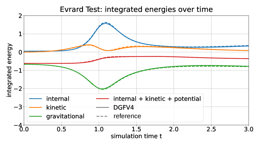
Figure 18: Domain-integrated energies over simulation time for the Evrard test run by our DGFV4 solver. The dashed lines show the reference solution computed with PPM on a uniform grid.

5.5 Coupling to TreeRay

Turbulent, multi-phase structures within the interstellar medium (ISM) are shaped by the complex and non-linear interplay between gravity, magnetic fields, heating and cooling, and the radiation and momentum input from stars (e.g. Agertz et al., 2013; Walch et al., 2015; Kim et al., 2017).

TreeRay (Wünsch et al., 2021) is a new radiation transport method combining an octree (Wünsch et al., 2018) with reverse ray tracing. The method is currently implemented in FLASH. In short, sources of radiation and radiation absorbing gas are mapped onto the tree encoded as emission and absorption coefficients. The tree is traversed for each grid cell and tree nodes are mapped onto rays going in all directions. Finally, a one-dimensional radiation transport equation is solved along each ray. Several physical processes are integrated into the TreeRay code by providing prescriptions for the absorption and the emission coefficients.

In this work, we employ a simple On-the-Spot approximation with only one source (a massive star) emitting a constant number of extreme ultraviolet (EUV) photons per unit time. The Spitzer sphere (Spitzer, 1978) is a simple model regarding the interaction of ionizing radiation with absorbing gases. In this model, the EUV radiation from a young, massive star ionizes and heats the surrounding medium, creating a so-called HII region, i.e. an over-pressured, expanding bubble of photo-ionized gas bounded by a sharp ionisation front (Whitworth, 1979; Deharveng et al., 2008). The expanding ionisation front drives a shock into the surrounding neutral, cold gas, sweeping it up into a dense, warm shell.

All radiation-hydrodynamic codes use this spherical expansion of an HII region as a standard test problem (Bisbas et al., 2015). The problem is insofar challenging, since it involves a complicated combination of fluid dynamics, radiative transfer, micro-physical heating, cooling, ionisation and recombination.

After we verify our simulation of the spherical expansion of an HII region with the Starbench test (Section 5.5.1), we extend the setup in order to simulate the expansion of an HII region into a fractal cloud (Section 5.5.2).

5.5.1 Starbench Test

Bisbas et al. (2015) introduced a standard benchmark test in 3D for early-time ($t\leq 0.05$ Myr) and late-time ($t>0.05$ Myr) expansion phases of the process. In this work we test our code with the 3D late expansion phase simulation which is coined the Starbench test.

An analytic approximation for the time evolution of the ionisation front (IF) is given by Spitzer (1978)

$$R_{\text{Spitzer}}(t)=R_{\text{S}}\left(1+\frac{7\,c_{\text{ionized}}\,t}{4\,R_{\text{S}}}\right)^{4/7}$$ (65)

where

$$R_{\text{S}}=\left(1+\frac{3\,\dot{N}\,m_{p}^{2}}{4\pi\,\alpha_{B}\,\rho_{0}^{2}}\right)^{1/3}$$ (66)

is the Strömgren radius (Strömgren, 1939), $c_{\text{ionized}}=12.85\,\text{km}\,\text{s}^{-1}$ is the sound speed in the ionised gas inside the isothermal bubble of $T_{\text{ionised}}=10^{4}\,\text{K}$. $\dot{N}=10^{49}\,\text{s}^{-1}$ is the rate at which the source at the centre emits hydrogen ionising photons ($E_{\nu}>13.6\text{eV}$), $m_{p}=1.67\cdot 10^{24}$ g is the proton mass, and $\alpha_{B}=2.7\cdot 10^{-13}\text{cm}^{3}\text{s}^{-1}$ is the recombination coefficient. The density of the surrounding neutral cloud of only hydrogen gas ($\gamma=5/3$) is taken to be $\rho_{0}=5.21\cdot 10^{-21}\text{g}\,\text{cm}^{-3}$ and has a temperature of $T_{\text{neutral}}=10^{3}\,\text{K}$. The corresponding sound speed is then $c_{\text{neutral}}=2.87\,\text{km}\,\text{s}^{-1}$. If, during the simulation, the temperature in the neutral gas exceeds $T_{\text{shell}}=300\,\text{K}$, it is instantaneously cooled to $T_{\text{shell}}$. Consequently, the shell of shock-compressed neutral gas immediately ahead of the expanding IF is effectively isothermal. The cooling aims to limit the thickness of the shell and make it resolvable for the numerical fluid solver. The given parameters result in a Strömgren radius of $R_{\text{S}}=0.3141\,\text{pc}$. Note, that this setup contains two fluid species, namely the neutral and ionised medium, and that all aforementioned physical and chemical processes are implemented within TreeRay which are completely opaque to the fluid solver.

Since the Spitzer solution (65) is only valid for the very early expansion phase, Bisbas et al. (2015) proposed a heuristic equation (equation (28) in Bisbas et al. (2015)) giving a good approximation of the position of the ionisation front at all times

$$R_{\text{Starbench}}=R_{\text{II}}+\big{(}1-0.733\,\exp(-t/\text{Myr})\big{)}\,(R_{\text{I}}-R_{\text{II}})$$ (67)

where $R_{\text{I}}$ and $R_{\text{II}}$ are solutions to the ordinary differential equations (8) and (12) in Bisbas et al. (2015). For brevity we omit the explicit definition of these and refer to the paper.

We run our simulation to final time $T=1.5\,\text{Myr}$ and set the domain to $\Omega=[0,3\,\text{pc}]^{3}$ which only represents one octant of the whole setup. Since the model is spherically symmetric around the emitting radiation source situated at the $\vec{x}=(0,0,0)^{T}$, we can speedup the simulation considerably. The resolution ranges from $32^{3}$ cells to $128^{3}$ cells. The boundaries of the domain touching the coordinate origin are reflecting walls while the rest are set to outflow. The ionised bubble is expected to occupy most of the domain by the end of the simulation.

Fig. 19 is a snapshot of the expanding bubble at time $t=0.8\,\text{Myr}$ showing a density slice at constant $z=0$. The dark violet region of lower density is completely filled with hot gas, photo-ionised by the radiation emitting point source sitting in the lower left corner. The dashed white circle demarks the ionisation front separating the inner, ionised medium from the surrounding, neutral medium of higher density. The dashed circle is computed with the Starbench solution (67) confirming excellent agreement between theoretical and numerical results.

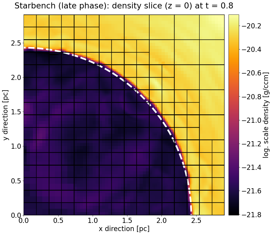
Figure 19: Density slice of the Starbench test setup at simulation time $t=0.8$ Myr computed with our DGFV4 solver and a maximum resolution of $256^{3}$ cells. The dashed circle highlights the Starbench solution given by (67). The black lines depict the AMR grid.

Additionally, we plotted the position of the ionisation front over the course of our simulation which we retrieved from snapshots taken at regular time intervals. The position of the IF is determined by calculating the mean radius where the shell-averaged ionised medium drops to 50 %, signalling the rapid transition to the neutral medium. The result is shown in Fig. 20 together with the Starbench solution (67) (black solid line) and the Spitzer solution (65) (grey dashed line). Clearly, our numerical solution matches the Spitzer solution only at very early times, but there is good agreement to the Starbench solution throughout the whole simulation. We ascribe the deviation observable from $t=1.1\,\text{Myr}$ on-wards to the bubble nearing the boundaries of the domain and the still rather low resolution. Investigations with identical parameters but different solvers in FLASH, such as PPM, revealed the exact same behaviour, hence the phenomenon is not rooted in our fluid solver.

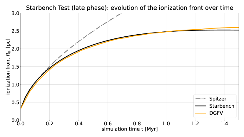
Figure 20: Ionisation fronts over time computed with our DGFV4 solver. For reference the Spitzer solution (65) and the Starbench solution (67) are plotted.

From a technical point of view, this particular test setup is remarkable, since it unites a large number of numerical components into one simulation. The complex interplay of physics and chemistry, especially the correct handling of a very sharp transition of a two-component (ionised/neutral) medium intertwined with ionisation, recombination, heating and cooling is a major challenge for every fluid dynamics code.

In our next section, we extend the Starbench test setup with an initial fractal density distribution to get a more realistic picture of a typical D-type expansion seen in astronomical observations.

5.5.2 D-type Expansion into a Fractal Molecular Cloud

Radiation driven feedback from massive stars is believed to be a key element in the evolution of molecular clouds. In this work, we utilise our new DGFV4 solver to model the dynamical effects of a single O7 star emitting ionising photons at $10^{49}\,\text{s}^{-1}$ located at the centre of a spherical molecular cloud. The cloud consists of $10^{4}\,\text{M}_{\odot}$ and stretches over a region of $6.4\,\text{pc}$ in each direction, so the volume-weighted mean density of the cloud amounts to $\rho_{0}=0.62\cdot 10^{-21}\,\text{g}\,\text{cm}^{-3}$.

It is a well established fact that molecular clouds are rich in internal structure probably driven by pure turbulence (Klessen, 2011; Girichidis et al., 2011) and subscribe to a statistically self-similar fractal structure (Stutzki et al., 1998). Our goal is to model the development of a molecular cloud having initial fractal dimension of $\mathcal{D}=2.6$ with a standard deviation of the approximately log-normal PDF of $\sigma_{\text{STD}}=0.38$. With these parameters the cloud is initially dominated by small-scale structures, which are then quickly overrun by the advancing ionisation front, thereby producing neutral pillars protruding into the HII region. The ionised gas within the expanding hot bubble blows out through a large number of small holes between these pillars. These regions are termed pillar-dominated (Walch et al., 2012).

Fractals with mass-size relations similar to those observed by Larson (1981) can be created in Fourier space (Shadmehri & Elmegreen, 2011), so we can freely configure the fractal dimension $\mathcal{D}$ of the initial cloud. A detailed account on how to construct such a fractal density distribution is presented in Walch et al. (2012).

The aspects of radiation physics are handled by the TreeRay module in FLASH which we introduced in detail before. Besides minor changes in setup parameters given below, this setup uses the same parameters as in Section 5.5.1. In contrast to Section 5.5.1, we simulate the whole expanding bubble, but keep the same maximum resolution at $128^{3}$ cells. Hence, the radiation source is at the centre of the cubic computational domain $\Omega=[-7\,\text{pc},7\,\text{pc}]^{3}$ and all boundaries are set to outflow. Radiative cooling effects of the molecular cloud itself are neglected. The result at final simulation time $T=1\,\text{Myr}$ can be seen in Fig. 21. The figure shows the column density in z-direction uncovering the aforementioned pillars as a product of the turbulent density distribution tearing apart the shell structure.

Since the setup combines multi-species and radiation physics in a very tough shock-turbulence regime, this final simulation shows that our new DG implementation in FLASH is capable of running complex multi-physics applications in astrophysical settings.

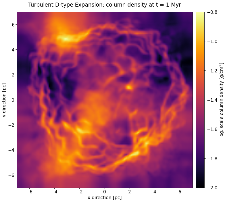
Figure 21: Turbulent D-type expansion into a fractal medium run by our DGFV4 solver. Shown is the column density along the z-axis: $\int_{z_{\mathrm{min}}}^{z_{\mathrm{max}}}\,\rho(x,y,z)\,\mathrm{d}z$.

6 Conclusions

In this paper, we discuss the implementation of a high-order DG fluid dynamics solver within the simulation framework FLASH, with a specific focus on multi-physics problems in astrophysics. We focus in particular on the modifications of the DG scheme to make it fit seamlessly within FLASH in such a way, that all other physics module can be naturally coupled without additional implementation overhead. A key to this is that our DG scheme uses mean value data organised into blocks. In specialised sections on different parts of the solver, we explain the strategy and compromises that we use to get a feasible implementation of the DG solver with the existing module interfaces of FLASH. The compromises are mainly related to accepting that the other physics modules assume mean value data (and not polynomial data), which means that some parts of the coupling are limited to second order accuracy, e.g., the evaluation of the gravitational source terms.

We demonstrate in extensive numerical tests that the novel DG implementation in FLASH works properly and is fully connected to all multi-physics modules. Step by step, the complexity of the test cases is increased by using setups that require more complex physical modules and features. Our novel DG solver in FLASH is ready for use in astrophysical simulations and thus ready for assessments and investigations.

Data Availability

The code is open source and can be accessed under github.com/jmark/DG-for-FLASH.

Appendix A Comparative Study for the MHD Torus Setup

Here we present a small comparative study of the MHD torus setup introduced in Section 5.4.1. We run a total of six simulations: three different resolutions of $64^{3}$, $128^{3}$, and $256^{3}$ cells each with the two MHD solvers Bouchut5 (Bouchut et al., 2010) and DGFV4. We use Bouchut5, a well-tested, second order, split solver in FLASH, since the standard solver for MHD, an unsplit, staggered mesh solver (Lee, 2013), crashes for this setup. As time integrator in DGFV4 we choose the third order, four stages SSP-RK(4,3) (Spiteri & Ruuth, 2002) scheme. All runs are conducted with the ODIN cluster (hosted at the computing centre at the University of Cologne) on 16 nodes each equipped with 16 Intel Xeon CPUs model E5-2670 (2.6 GHz). This gives a total cpu count (#cpus) of 256 cores.

The results at final simulation time are shown in Fig. 22 and Fig. 23. Clearly, the DGFV4 solver shows finer structures and more scales in the disk at every resolution level compared to Bouchut5 and is capable to resolve magneto-rotationally driven outflows at lowest resolution levels.

In Table 3 we list the runtimes of all six simulations. Bouchut5 is a split solver and thus in general has a larger time step (about a factor of 2) compared to unsplit schemes. Hence, the number of time steps (#steps) are lower for Bouchut5 compared to DGFV4, which results in overall faster completion times for the same resolution. To further assess our implementation, we compute a performance index (PID) as

$$\mathrm{PID}=(\mathrm{runtime}\,\times\,\#\mathrm{cpus})\,/\,(\#\mathrm{cells}\,\times\,\#\mathrm{steps})$$ (68)

which we also list in Table 3. PID is basically the average cost of a spatial cell per time step. A lower PID means better performance. Note, that the MPI-parallelised code scales better with increasing resolution resulting in lower PIDs for both schemes. A drawback of DG schemes compared to FV discretizations is, that the spatial operator spectra are more stiff and hence need more stable time integration methods, such as the high-order RK method used in this comparison. This means, that the DGFV4 discretization has to be called four times per time step. Factoring this in and comparing the CPU time per evaluation of the spatial operator gives an unexpected result. The novel DGFV4 implementation is quicker than the Bouchut5 implementation, as one has to divide the PID of DGFV4 by a factor of four to get the cost of a spatial grid cell per ’sweep’.

Table 3: Runtimes of the MHD torus setup introduced in Section 5.4.1 for the Bouchut5 and our DGFV4 solver implemented in FLASH (v4.3.). All simulations run on the cluster ODIN on 16 nodes á 16 cores. The definition for the performance index (PID) is given by eqn. (68).

solver	#cells	runtime [h]	#steps	PID [$\mu$s]
Bouchut5	$64^{3}$	0.03	940	110.00
	$128^{3}$	0.41	3012	60.16
	$256^{3}$	6.14	8374	40.26
DGFV4	$64^{3}$	0.08	1736	156.10
	$128^{3}$	1.18	4808	107.80
	$256^{3}$	17.24	13898	68.16

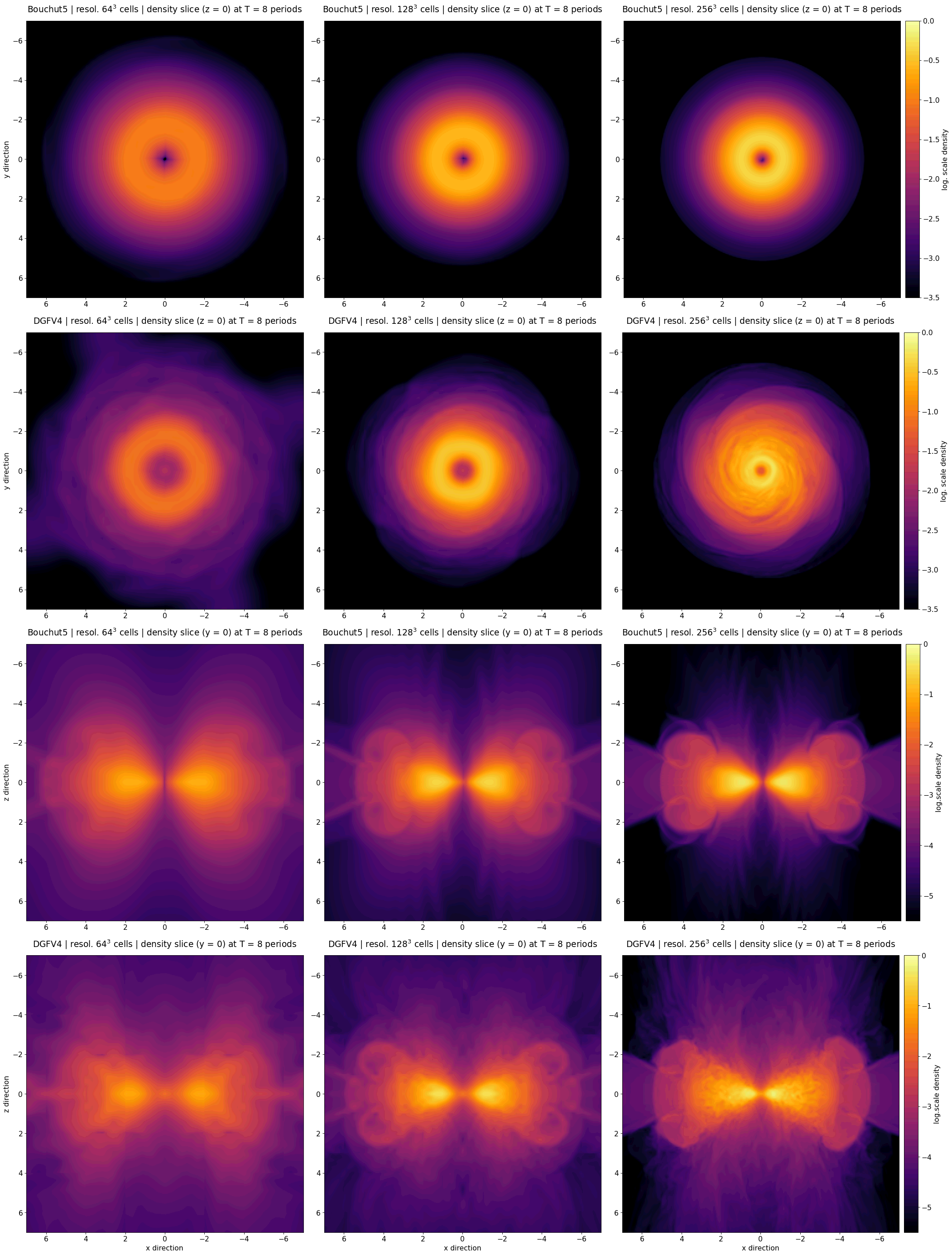
Figure 22: MHD torus after 8 periods run for max. resolutions (from left to right) $64^{3}$, $128^{3}$, $256^{3}$ and two fluid solvers Bouchut5 (rows 1,3) and DGFV4 (rows 2,4). Shown are log-scale density slices in the x-y plane (rows 1,2) and in the x-z plane (rows 3,4).

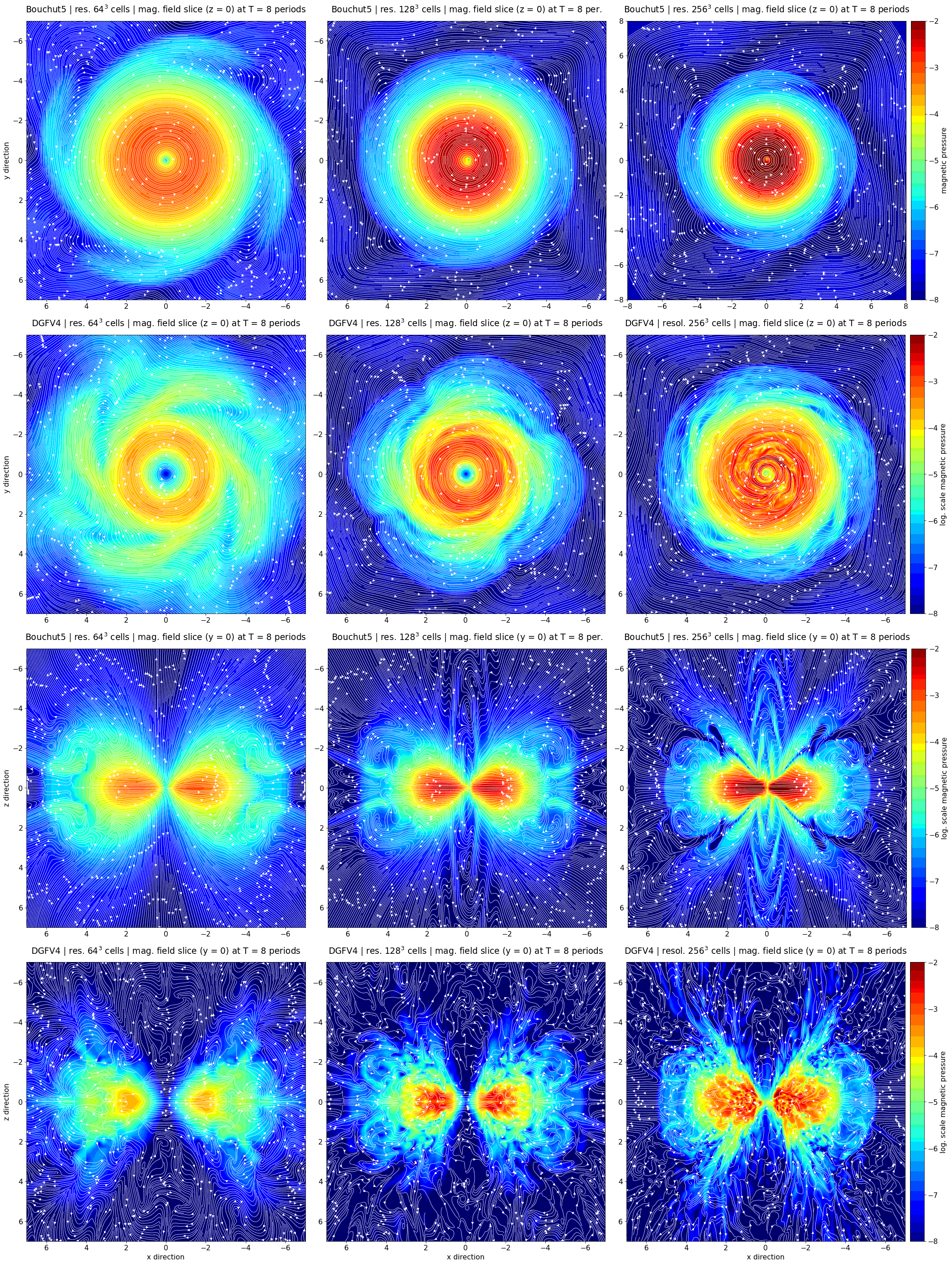
Figure 23: MHD torus after 8 periods run for max. resolutions (from left to right) $64^{3}$, $128^{3}$, $256^{3}$ and two fluid solvers Bouchut5 (rows 1,3) and DGFV4 (rows 2,4). Shown are log-scale magnetic pressure slices in the x-y plane (rows 1,2) and in the x-z plane (rows 3,4). The streamlines in white denote the magnetic field lines.

References

- Agertz et al. (2013) Agertz O., Kravtsov A. V., Leitner S. N., Gnedin N. Y., 2013, The Astrophysical Journal, 770, 25
- Ainsworth (2004) Ainsworth M., 2004, Journal of Computational Physics, 198, 106
- Balbus & Hawley (1990) Balbus S. A., Hawley J. F., 1990, in Bulletin of the American Astronomical Society. p. 1209
- Balsara (2017) Balsara D. S., 2017, Living reviews in computational astrophysics, 3, 1
- Balsara & Spicer (1999) Balsara D. S., Spicer D. S., 1999, Journal of Computational Physics, 149, 270
- Balsara et al. (2009) Balsara D. S., Rumpf T., Dumbser M., Munz C.-D., 2009, Journal of Computational Physics, 228, 2480
- Barnes & Hut (1986) Barnes J., Hut P., 1986, nature, 324, 446
- Bassi et al. (2005) Bassi F., Crivellini A., Rebay S., Savini M., 2005, Computers & Fluids, 34, 507
- Bauer et al. (2016) Bauer A., Schaal K., Springel V., Chandrashekar P., Pakmor R., Klingenberg C., 2016, in , Software for Exascale Computing-SPPEXA 2013-2015. Springer, pp 381–402
- Bisbas et al. (2015) Bisbas T. G., et al., 2015, Monthly Notices of the Royal Astronomical Society, 453, 1324
- Bohm et al. (2018) Bohm M., Winters A. R., Gassner G. J., Derigs D., Hindenlang F., Saur J., 2018, Journal of Computational Physics
- Bohm et al. (2019) Bohm M., Schermeng S., Winters A. R., Gassner G. J., Jacobs G. B., 2019, Journal of Scientific Computing, 81, 820
- Bouchut et al. (2010) Bouchut F., Klingenberg C., Waagan K., 2010, Numerische Mathematik, 115, 647
- Brackbill & Barnes (1980) Brackbill J. U., Barnes D. C., 1980, Journal of Computational Physics, 35, 426
- Brio & Wu (1988) Brio M., Wu C. C., 1988, Journal of computational physics, 75, 400
- Burns et al. (2020) Burns K. J., Vasil G. M., Oishi J. S., Lecoanet D., Brown B. P., 2020, Physical Review Research, 2, 023068
- Chandrasekhar (1960) Chandrasekhar S., 1960, Proceedings of the National Academy of Sciences of the United States of America, 46, 253
- Chandrashekar & Klingenberg (2016) Chandrashekar P., Klingenberg C., 2016, SIAM Journal on Numerical Analysis, 54, 1313
- Ching et al. (2019) Ching E. J., Lv Y., Gnoffo P., aichael Barnhardt Ihme M., 2019, Journal of Computational Physics, 376, 54
- Cockburn & Shu (1998) Cockburn B., Shu C.-W., 1998, Journal of Computational Physics, 141, 199
- Cockburn et al. (1990) Cockburn B., Hou S., Shu C.-W., 1990, Mathematics of Computation, 54, 545
- Colella & Woodward (1984) Colella P., Woodward P. R., 1984, Journal of computational physics, 54, 174
- Colella et al. (2009) Colella P., Graves D. T., Ligocki T., Martin D., Modiano D., Serafini D., Van Straalen B., 2009, Available at the Chombo website: http://seesar. lbl. gov/ANAG/chombo/(September 2008)
- Collins et al. (2010) Collins D. C., Xu H., Norman M. L., Li H., Li S., 2010, The Astrophysical Journal Supplement Series, 186, 308
- Daley et al. (2012) Daley C., Vanella M., Dubey A., Weide K., Balaras E., 2012, Concurrency and Computation: Practice and Experience, 24, 2346
- Dedner et al. (2002) Dedner A., Kemm F., Kröner D., Munz C.-D., Schnitzer T., Wesenberg M., 2002, Journal of Computational Physics, 175, 645
- Deharveng et al. (2008) Deharveng L., Lefloch B., Kurtz S., Nadeau D., Pomares M., Caplan J., Zavagno A., 2008, Astronomy & Astrophysics, 482, 585
- Derigs et al. (2016) Derigs D., Winters A. R., Gassner G. J., Walch S., 2016, Journal of Computational Physics, 317, 223
- Derigs et al. (2018) Derigs D., Winters A. R., Gassner G. J., Walch S., Bohm M., 2018, Journal of Computational Physics, 364, 420
- Després & Labourasse (2015) Després B., Labourasse E., 2015, Journal of Computational Physics, 290, 28
- Dobrev et al. (2012) Dobrev V. A., Kolev T. V., Rieben R. N., 2012, SIAM Journal on Scientific Computing, 34, B606
- Dumbser & Loubere (2016) Dumbser M., Loubere R., 2016, Journal of Computational Physics, 319, 163
- Dumbser et al. (2014) Dumbser M., Zanotti O., Loubere R., Diot S., 2014, Journal of Computational Physics, 278, 47
- Evans & Hawley (1988) Evans C. R., Hawley J. F., 1988, The Astrophysical Journal, 332, 659
- Evrard (1988) Evrard A. E., 1988, Monthly Notices of the Royal Astronomical Society, 235, 911
- Fromang et al. (2006) Fromang S., Hennebelle P., Teyssier R., 2006, Astronomy & Astrophysics, 457, 371
- Fryxell et al. (2000) Fryxell B., et al., 2000, The Astrophysical Journal Supplement Series, 131, 273
- Gaburov & Nitadori (2011) Gaburov E., Nitadori K., 2011, Monthly Notices of the Royal Astronomical Society, 414, 129
- Gardiner & Stone (2005) Gardiner T. A., Stone J. M., 2005, Journal of Computational Physics, 205, 509
- Gassner & Kopriva (2011) Gassner G., Kopriva D. A., 2011, SIAM Journal on Scientific Computing, 33, 2560
- Gatto et al. (2015) Gatto A., et al., 2015, Monthly Notices of the Royal Astronomical Society, 449, 1057
- Girichidis et al. (2011) Girichidis P., Federrath C., Banerjee R., Klessen R. S., 2011, Monthly Notices of the Royal Astronomical Society, 413, 2741
- Glover & Clark (2014) Glover S. C., Clark P. C., 2014, Monthly Notices of the Royal Astronomical Society, 437, 9
- Godunov (1972) Godunov S., 1972, Numerical Methods for Mechanics of Continuum Medium, 1, 26
- Gouasmi et al. (2020) Gouasmi A., Duraisamy K., Murman S. M., 2020, Computer Methods in Applied Mechanics and Engineering, 363, 112912
- Guillet et al. (2019) Guillet T., Pakmor R., Springel V., Chandrashekar P., Klingenberg C., 2019, Monthly Notices of the Royal Astronomical Society, 485, 4209
- Guo et al. (2015) Guo W., Nair R. D., Zhong X., 2015, International Journal for Numerical Methods in Fluids, 81, 3
- He et al. (2020) He X., Yang D., Huang X., Ma X., 2020, Geophysics, 85, T101
- Karni (1994) Karni S., 1994, Journal of Computational Physics, 112, 31
- Karniadakis & Sherwin (2005) Karniadakis G. E., Sherwin S. J., 2005, Spectral/hp Element Methods for Computational Fluid Dynamics. Oxford University Press
- Kemm (2013) Kemm F., 2013, Communications in Applied Mathematics and Computational Science, 8, 1
- Kidder et al. (2017) Kidder L. E., et al., 2017, Journal of Computational Physics, 335, 84
- Kim et al. (2017) Kim J.-G., Kim W.-T., Ostriker E. C., Skinner M. A., 2017, The Astrophysical Journal, 851, 93
- Klessen (2011) Klessen R. S., 2011, EAS Publications Series, 51, 133
- Kopriva (2009) Kopriva D. A., 2009, Implementing spectral methods for partial differential equations: Algorithms for scientists and engineers. Springer Science & Business Media
- Kopriva et al. (2002) Kopriva D. A., Woodruff S. L., Hussaini M. Y., 2002, International Journal for Numerical Methods in Engineering, 53, 105
- Kuzmin (2012) Kuzmin D., 2012, International Journal for Numerical Methods in Fluids, 71, 1178
- Larson (1981) Larson R. B., 1981, Monthly Notices of the Royal Astronomical Society, 194, 809
- Lee (2013) Lee D., 2013, Journal of Computational Physics, 243, 269
- Li et al. (2021) Li P. S., et al., 2021, Journal of Open Source Software, 6, 3771
- Lombart & Laibe (2020) Lombart M., Laibe G., 2020, Monthly Notices of the Royal Astronomical Society, 501, 4298
- Machida et al. (1999) Machida M., Hayashi M., Matsumoto R., 1999, in Star Formation 1999. pp 245–246
- Manzanero et al. (2018) Manzanero J., Ferrer E., Rubio G., Valero E., 2018, Journal of Computational Physics
- Markert et al. (2021) Markert J., Gassner G., Walch S., 2021, Communications on Applied Mathematics and Computation, pp 1–43
- Mignone et al. (2012) Mignone A., Flock M., Stute M., Kolb S., Muscianisi G., 2012, Astronomy & Astrophysics, 545, A152
- Mocz et al. (2014) Mocz P., Vogelsberger M., Sijacki D., Pakmor R., Hernquist L., 2014, Monthly Notices of the Royal Astronomical Society, 437, 397
- Moura et al. (2017) Moura R. C., Mengaldo G., Peiró J., Sherwin S. J., 2017, Journal of Computational Physics, 330, 615
- Müller & Steinmetz (1995) Müller E., Steinmetz M., 1995, Computer Physics Communications, 89, 45
- Munz et al. (2007) Munz C.-D., Dumbser M., Roller S., 2007, Journal of Computational Physics, 224, 352
- Murawski (2002) Murawski K., 2002, Analytical and numerical methods for wave propagation in fluid media. A Vol. 7, World Scientific
- Okada et al. (1989) Okada R., Fukue J., Matsumoto R., 1989, Publications of the Astronomical Society of Japan, 41, 133
- Olson et al. (1999) Olson K., MacNeice P., Fryxell B., Ricker P., Timmes F., Zingale M., 1999, in American Astronomical Society Meeting Abstracts. pp 42–03
- Orszag & Tang (1979) Orszag S. A., Tang C.-M., 1979, Journal of Fluid Mechanics, 90, 129
- Parker (1966) Parker E., 1966, The Astrophysical Journal, 145, 811
- Persson & Peraire (2006) Persson P.-O., Peraire J., 2006, in 44th AIAA Aerospace Sciences Meeting and Exhibit. American Institute of Aeronautics and Astronautics
- Powell et al. (1999) Powell K. G., Roe P. L., Linde T. J., Gombosi T. I., De Zeeuw D. L., 1999, Journal of Computational Physics, 154, 284
- Qiu & Zhu (2010) Qiu J., Zhu J., 2010, in , Notes on Numerical Fluid Mechanics and Multidisciplinary Design. Springer Berlin Heidelberg, pp 67–80
- Ralston (1962) Ralston A., 1962, Mathematics of computation, 16, 431
- Rastätter et al. (1994) Rastätter L., Voge A., Schindler K., 1994, Physics of plasmas, 1, 3414
- Ricker (2008) Ricker P., 2008, The Astrophysical Journal Supplement Series, 176, 293
- Rueda-Ramírez et al. (2021) Rueda-Ramírez A. M., Hennemann S., Hindenlang F. J., Winters A. R., Gassner G. J., 2021, Journal of Computational Physics, 444, 110580
- Ryu et al. (1998) Ryu D., Miniati F., Jones T., Frank A., 1998, The Astrophysical Journal, 509, 244
- Schaal et al. (2015) Schaal K., Bauer A., Chandrashekar P., Pakmor R., Klingenberg C., Springel V., 2015, Monthly Notices of the Royal Astronomical Society, 453, 4278
- Shadmehri & Elmegreen (2011) Shadmehri M., Elmegreen B. G., 2011, Monthly Notices of the Royal Astronomical Society, 410, 788
- Shu & Osher (1988) Shu C.-W., Osher S., 1988, Journal of computational physics, 77, 439
- Sonntag & Munz (2014) Sonntag M., Munz C.-D., 2014, in , Finite Volumes for Complex Applications VII-Elliptic, Parabolic and Hyperbolic Problems. Springer International Publishing, pp 945–953
- Spiteri & Ruuth (2002) Spiteri R. J., Ruuth S. J., 2002, SIAM Journal on Numerical Analysis, 40, 469
- Spitzer (1978) Spitzer L., 1978, Physical processes in the interstellar medium. John Wiley & Sons
- Springel (2010) Springel V., 2010, Proceedings of the International Astronomical Union, 6, 203
- Springel et al. (2001) Springel V., Yoshida N., White S. D., 2001, New Astronomy, 6, 79
- Stone et al. (2008) Stone J. M., Gardiner T. A., Teuben P., Hawley J. F., Simon J. B., 2008, The Astrophysical Journal Supplement Series, 178, 137
- Stone et al. (2020) Stone J. M., Tomida K., White C. J., Felker K. G., 2020, The Astrophysical Journal Supplement Series, 249, 4
- Strömgren (1939) Strömgren B., 1939, ApJ, 89, unknown
- Stutzki et al. (1998) Stutzki J., Bensch F., Heithausen A., Ossenkopf V., Zielinsky M., 1998, Astronomy and Astrophysics, 336, 697
- Susanto (2014) Susanto A., 2014, High-Order Finite-Volume Schemes for Magnetohydrodynamics. University of Waterloo, Waterloo, Ontario, Canada
- Toro (1999) Toro E. F., 1999, Riemann Solvers and Numerical Methods for Fluid Dynamics. Springer Verlag
- Tóth (2000) Tóth G., 2000, Journal of Computational Physics, 161, 605
- Velikhov (1959) Velikhov E., 1959, Sov. Phys. JETP, 36, 995
- Vilar (2019) Vilar F., 2019, Journal of Computational Physics, 387, 245
- Walch et al. (2012) Walch S., Whitworth A., Bisbas T., Wünsch R., Hubber D., 2012, Monthly Notices of the Royal Astronomical Society, 427, 625
- Walch et al. (2015) Walch S., et al., 2015, Monthly Notices of the Royal Astronomical Society, 454, 238
- Warburton & Karniadakis (1999) Warburton T., Karniadakis G. E., 1999, Journal of computational Physics, 152, 608
- Wetzstein et al. (2009) Wetzstein M., Nelson A. F., Naab T., Burkert A., 2009, The Astrophysical Journal Supplement Series, 184, 298
- Whitworth (1979) Whitworth A., 1979, Monthly Notices of the Royal Astronomical Society, 186, 59
- Winters & Gassner (2016) Winters A. R., Gassner G. J., 2016, Journal of Scientific Computing, 67, 514
- Wünsch et al. (2018) Wünsch R., Walch S., Dinnbier F., Whitworth A., 2018, Monthly Notices of the Royal Astronomical Society, 475, 3393
- Wünsch et al. (2021) Wünsch R., Walch S., Dinnbier F., Seifried D., Haid S., Klepitko A., Whitworth A. P., Palouš J., 2021, Monthly Notices of the Royal Astronomical Society, 505, 3730
- Zanotti et al. (2015) Zanotti O., Fambri F., Dumbser M., Hidalgo A., 2015, Computers & Fluids, 118, 204
- Zhang & Stanescu (2010) Zhang X., Stanescu D., 2010, Computers & Fluids, 39, 251
- Zhu & Qiu (2009) Zhu J., Qiu J., 2009, Journal of Scientific Computing, 39, 293