SDSS-IV MaNGA: Understanding Ionized Gas Turbulence using Integral Field Spectroscopy of 4500 Star-Forming Disk Galaxies

Abstract

The Sloan Digital Sky Survey MaNGA program has now obtained integral field spectroscopy for over 10,000 galaxies in the nearby universe. We use the final MaNGA data release DR17 to study the correlation between ionized gas velocity dispersion and galactic star formation rate, finding a tight correlation in which $\sigma_{\rm H\alpha}$ from galactic HII regions increases significantly from $\sim 18-30$ km s${}^{-1}\,$ broadly in keeping with previous studies. In contrast, $\sigma_{\rm H\alpha}$ from diffuse ionized gas (DIG) increases more rapidly from $20-60$ km s${}^{-1}\,$. Using the statistical power of MaNGA, we investigate these correlations in greater detail using multiple emission lines and determine that the observed correlation of $\sigma_{\rm H\alpha}$ with local star formation rate surface density is driven primarily by the global relation of increasing velocity dispersion at higher total SFR, as are apparent correlations with stellar mass. Assuming HII region models consistent with our finding that $\sigma_{\textrm{[O\,{\sc iii}]}}<\sigma_{\rm H\alpha}<\sigma_{\textrm{[O\,{\sc i}]}}$, we estimate the velocity dispersion of the molecular gas in which individual HII regions are embedded, finding values $\sigma_{\rm Mol}=5-30$ km s${}^{-1}\,$ consistent with ALMA observations in a similar mass range. Finally, we use variations in the relation with inclination and disk azimuthal angle to constrain the velocity dispersion ellipsoid of the ionized gas $\sigma_{z}/\sigma_{r}=0.84\pm 0.03$ and $\sigma_{\phi}/\sigma_{r}=0.91\pm 0.03$, similar to that of young stars in the Galactic disk. Our results are most consistent with theoretical models in which turbulence in modern galactic disks is driven primarily by star formation feedback.

I. Introduction

The gaseous interstellar medium (ISM) extends throughout galaxies, the densest molecular phase of which is closely confined to the midplane of the galactic disk. The distribution of this gas is far from uniform though; periodically localized overdensities become sufficiently massive that their gravity can overcome hydrostatic gas pressure and trigger bursts of star formation. The bright O and B stars produced by this star formation ionize the surrounding ISM on the timescale of a few Myr, illuminating these regions in nebular emission lines such as $\rm H\alpha$, [N ii]$\lambda 6585$, and [O iii] $\lambda 5007$ that can be observed to cosmological distances. On small scales, the gas velocity dispersion observed in such emission lines can tell us about the physical conditions within individual HII regions. On large scales $\sim$ a few hundred pc to a kpc, such dispersions also encode information about the overall structure of the molecular gas disk in which the HII regions are embedded; the corresponding turbulence is thus tightly linked to the overall stability of the gaseous disk.

One of the major puzzles revealed by observations in recent years is the apparent systematic growth of turbulence with redshift. As traced by observations of bright nebular emission lines, numerous studies (e.g., Glazebrook, 2013; Simons et al., 2017; Johnson et al., 2018; Übler et al., 2019) have confirmed a systematic increase of the velocity dispersion $\sigma_{\rm H\alpha}$ from $\sim 20$ km s${}^{-1}\,$at $z=0$ (Terlevich & Melnick, 1981; Epinat et al., 2008; Varidel et al., 2016; Zhou et al., 2017) to $\sim 70$ km s${}^{-1}\,$at $z\sim 2-3$ (e.g., Law et al., 2009; Förster Schreiber et al., 2009, 2018; Jones et al., 2010; Price et al., 2020). Indeed, in the $z\sim 2$ universe many typical star forming galaxies exhibit kinematics that are dominated by turbulent motion, even in cases for which the galaxy morphology exhibits unambiguous spiral disk structure (Law et al., 2012) (although c.f. Yuan et al., 2017).

The cause of this strong evolution in turbulence is uncertain (see review by Glazebrook, 2013) but has been broadly ascribed either to increased radiative and mechanical feedback from intense star formation (e.g., Lehnert et al., 2009; Green et al., 2014; Moiseev et al., 2015) or gravitational instabilities driven by galactic gas accretion (e.g., Dekel et al., 2009; Ceverino et al., 2010; Krumholz & Burkhart, 2016), both of which predict a degree of correlation between $\sigma_{\rm H\alpha}$ and the total galactic star formation rate. Distinguishing between these two scenarios is challenging; in the high-redshift universe the entire star-forming main sequence is offset to significantly higher star formation rates (SFR) at fixed stellar mass compared to $z=0$ (see, e.g., Wuyts et al., 2011), and at the same time models also suggest the likelihood of significant gas accretion from clumpy cold streams (e.g., Dekel et al., 2009; Ceverino et al., 2010). In the nearby universe ultraluminous galaxies with high SFR possess much higher $\sigma_{\rm H\alpha}$ than their main sequence counterparts, yet localized peaks in the velocity dispersion tend to be associated with large-scale gas flows rather than peaks in the star formation rate surface density (e.g., Colina et al., 2005; Arribas et al., 2014).

Generally, the large statistical studies of spectroscopic galaxy properties at $z\sim 0$ around which such studies are anchored are based on spatially unresolved fiber spectroscopy (e.g., Brinchmann et al., 2004) for which $\sigma_{\rm H\alpha}$ can be both biased by contributions from active galactic nuclei (AGN) and challenging to separate from large-scale streaming and rotational motions. Similarly, targeted spatially-resolved observations have by necessity focused on relatively small samples of objects (e.g., Andersen et al., 2006; Epinat et al., 2010; Martinsson et al., 2013; Arribas et al., 2014; Moiseev et al., 2015; Varidel et al., 2016) that trace only subsets of the star forming main sequence.

The early generation of IFU galaxy surveys has likewise not been able to address this question; the $R=850$ spectral resolution of the Calar Alto Legacy Integral Field Area Survey (CALIFA; Sánchez et al., 2012) was too low to be able to measure $\rm H\alpha$ velocity dispersions of typical galactic disks, while the $R\sim 1200$ Atlas3D survey (Cappellari et al., 2011) focused exclusively on early-type galaxies. With the current generation of large-scale IFU galaxy survey such as MaNGA (Bundy et al., 2015) and SAMI (Croom et al., 2012) , it has now become possible for the first time to study statistically large representative samples of nearby galaxies with IFU observations similar to those employed at high redshifts. The MaNGA survey in particular represents more than an order of magnitude increase in sample size compared to previous IFU surveys, with a now-completed sample of $>$ 10,000 galaxies and contiguous spectral coverage in the wavelength range $\lambda\lambda 0.36-1.0\micron$). However, the $R\sim 2000$ spectral resolution of MaNGA (corresponding to an instrumental resolution with $1\sigma$ width $\sim 70$ km s${}^{-1}\,$) makes it challenging to study velocity dispersions that are typically on the order of $20-30$ km s${}^{-1}\,$.

In Law et al. (2021a) we showed that through a multi-year concerted effort to understand and model the properties of the MaNGA instrument, pipeline estimates of the instrumental line spread function (LSF) in the final DR17 survey data products are accurate to within 0.3% systematic and 2% random error, permitting the reliable study of astrophysical velocity dispersions down to 20 km s${}^{-1}\,$and below. Further, in Law et al. (2021b) we showed that these astrophysical velocity dispersions exhibit dramatic trends with the physical origin of the ionizing photons exciting the gas, with star-formation activity preferentially occurring in dynamically cold disks with a well defined peak in the galactic line-of-sight velocity distribution around 25 km s${}^{-1}\,$ and AGN/LI(N)ER activity preferentially illuminating gas with much larger velocity dispersions extending to 200 km s${}^{-1}\,$ and above. In this third paper of the series, we focus on subtle variations in velocity dispersion within the star-forming sequence and the underlying relation to the galactic star formation rate as a local benchmark for future observations at high redshift.

We structure our discussion as follows. In §II we discuss the characteristics of the MaNGA galaxy sample and the relevant survey data products, and select a subset of spaxels whose line ratios are consistent with ionization by galactic HII regions. In §III we present the basic correlations between $\sigma_{\rm H\alpha}$ and star formation rate noting the effect of beam smearing, and compare our results against recent works in the literature. In §IV we use the statistical power of MaNGA to dissect the contributions from star formation rate, stellar mass, and other observables in order to isolate the physical mechanism responsible for the observed correlations. We investigate the role of galaxy inclination in §V, and in combination with galaxy azimuthal information measure the ellipsoid of the ionized gas velocity dispersion field. Finally, in §VI we discuss the implications of our results for the structure of galactic HII regions, the underlying molecular gas, and for the diffuse ionized gas. We summarize our conclusions in §VII.

Throughout our analysis we adopt a Chabrier (2003) stellar initial mass function and a $\Lambda$CDM cosmology in which $H_{0}=70$ km s^-1 Mpc^-1, $\Omega_{m}=0.27$, and $\Omega_{\Lambda}=0.73$.

II. Observational Data

II.1. Survey Overview and Data Products

The Mapping Nearby Galaxies at APO (MaNGA, Bundy et al., 2015) survey is one of three primary surveys undertaken as part of the fourth-generation Sloan Digital Sky Survey (SDSS-IV, Blanton et al., 2017) that uses a multiplexed IFU fiber bundle interface (Drory et al., 2015) to feed the BOSS spectrographs (Smee et al., 2013) on the Sloan 2.5m telescope (Gunn et al., 2006) at Apache Point Observatory. MaNGA survey operations (Law et al., 2015; Yan et al., 2016) began in 2014 and concluded in 2020, providing $R\sim 2000$ resolved spectroscopy in the wavelength range $\lambda\lambda 3600-10300$ Å for $>10,000$ unique galaxies (see Law et al., 2021a, their Table 1). These raw observational data have been fully processed using the MaNGA Data Reduction Pipeline (DRP) to produce science-grade calibrated data products (Law et al., 2016, 2021a; Yan et al., 2016), the final version of which was available internally to the SDSS-IV collaboration as version MPL-11 and released to the broader astronomical community as SDSS Data Release 17 (DR17; Abdurro’uf et al., 2021) in December 2021.

Following Law et al. (2021a) and Law et al. (2021b), we use the $\rm H\alpha$ velocity dispersion maps produced by the MaNGA Data Analysis Pipeline (DAP, Belfiore et al., 2019; Westfall et al., 2019). The stellar continuum templates used for fitting the emission lines were based on hierarchically clustered template spectra observed by the MaNGA MaStar program (Yan et al., 2019). These DAP velocity dispersion maps provide raw line widths, from which we subtracted the expected instrumental LSF (also provided by the DAP) in quadrature. We additionally corrected these maps for beam smearing arising from the finite size of the MaNGA PSF by following the method described by Law et al. (2021a) and Law et al. (2021b) (see their §5 and §2 respectively) in which a model velocity field for each galaxy is convolved with the PSF to estimate the artificial inflation in the observed velocity dispersions.

As discussed at length by Law et al. (2021a) these DR17-based velocity dispersions are significantly more reliable than the values provided in previous MaNGA public data releases.

II.2. MaNGA Galaxy Sample

The full MaNGA galaxy sample is highly heterogenous and spans galaxies of a wide range of masses and morphological types with a nearly flat mass distribution in the range $M_{\ast}=10^{9}-10^{11}M_{\odot}$. This full sample is composed of a primary galaxy sample that covers a radial range out to 1.5 effective radii ($R_{\rm e}$), a secondary sample that covers out to 2.5 $R_{\rm e}$, a color-enhanced sample that fills in less-represented regions of color/magnitude space, and a variety of ancillary programs that have their own unique selection criteria (e.g., massive galaxies, dwarf galaxies, Milky Way analogs, bright AGN, post starburst galaxies, etc). In the present contribution we are most interested in the properties of star forming regions within star forming galaxies, and must therefore downselect from the full sample.

Starting with the 11,273 galaxy data cubes in DR17, we follow Law et al. (2021b, see their Section 2) in rejecting nearby galaxies ($z<0.001$), mis-centered galaxies, galaxies with data quality problems, and a small number of unusual galaxies in the Coma cluster. This leaves a sample of 10,016 data cubes corresponding to 9883 unique galaxies. Next, we downselect to include only star-forming galaxies as identified by their mean $\rm H\alpha$ equivalent width measured within 1 effective radius ($R_{\rm e}$) of the galaxy center. As illustrated in Law et al. (2021b, see their Figure 1), our requirement of $EW_{\rm H\alpha}>5$ Å does a good job of selecting galaxies that lie on the star-forming main sequence, eliminating those in both the red sequence ($EW_{\rm H\alpha}<2$ Å) and the transitional ‘green valley’ (2 Å $<EW_{\rm H\alpha}<5$ Å) and reducing our total sample to 5142 galaxy data cubes.

As discussed further in §V, we make no specific cuts on galaxy disk inclination to the line of sight in order to explore the impact of inclination on our results.

II.3. Selecting Star-Forming Spaxels

While we have thus identified our galaxy sample, we must additionally restrict our study to those spaxels within these galaxies whose $\rm H\alpha$ emission is dominated by ionizing photons arising from star-forming HII regions. As we explored in depth in Law et al. (2021b), resolved $\rm H\alpha$ velocity dispersions from the entire MaNGA sample ($\sim 3.6$ million spaxels across 7400 individual galaxies) exhibit a clear two-component kinematic population consisting of a dynamically cold gas disk (LOSVDs with a strong peak around $\sigma_{\rm H\alpha}=24$ km s${}^{-1}\,$) and an extended warm tail (LOSVDs extending to $\sigma_{\rm H\alpha}>100$ km s${}^{-1}\,$). These two populations are strongly segregated from each other by their strong-line nebular flux ratios (e.g., [N ii]/$\rm H\alpha$, [S ii]/$\rm H\alpha$, [O iii]/$\rm H\beta$, and [O i]/$\rm H\alpha$) the boundary between which is traced by a series of well defined curves (see Law et al., 2021b, their Eqns. 1-3). For the [S ii]/$\rm H\alpha$ vs [O iii]/$\rm H\beta$ relation in particular, these kinematically defined curves are in excellent agreement with theoretical relations (e.g., Kewley et al., 2001), indicating that selecting spaxels according to their strong emission line ratios is a reliable way of identifying dynamically cold star-forming gas disks.

We therefore make our initial identification of star-forming spaxels by selecting those whose [S ii]/$\rm H\alpha$ vs [O iii]/$\rm H\beta$ line ratios place them below the relation defined by Law et al. (2021b, their Eqn. 2):

$$R3=\frac{0.648}{S2-0.324}+1.349$$ (1)

for $R3\equiv\textrm{log}(\textrm{[O\,{\sc iii}]}\ \lambda 5007/\rm H\beta)$ and $S2\equiv\textrm{log}(\textrm{[S\,{\sc ii}]}\ \lambda 6716+\lambda 6731/\rm H\alpha)$. As discussed by Law et al. (2021b, see their §5.4 and Figure 9) this selection cut is broadly similar to the criterion defined by Kewley et al. (2001), except slightly offset to larger $S2$ in order to compensate for star-forming spaxels at large galactocentric radii that were missing from early work using SDSS single-fiber spectra against which the Kewley et al. (2001) study was calibrated.

As our goal is to diagnose statistical trends in actively star-forming galaxies for which $\sigma_{\rm H\alpha}$ is typically $\leq 30$ km s${}^{-1}\,$, we additionally restrict our sample to spaxels with $\rm H\alpha$ signal-to-noise ratio (SNR) $>50$ and that lie at radii $>4$ arcsec from the center of each galaxy. The first of these cuts is necessary in order to avoid systematic bias in the recovered velocity dispersions arising from the preferential loss of spaxels whose measured line widths scatter below the instrumental resolution at low SNR (see discussion in Law et al., 2021a, their §4.3 and Figure 15). The second of these cuts allows us to mitigate additional systematic biases that arise from beam smearing by the observational PSF, which is most pronounced in the central regions of galaxies. Although we have corrected the DAP velocity dispersion maps for beam smearing following the method outlined by Law et al. (2021a, their §5), as these authors note the corrected values are most uncertain within the central 4 arcsec. Additionally, we require the [S ii], [O iii], and $\rm H\beta$ lines to be detected at SNR $>3$ to avoid contamination by low-SNR line ratios, and $\sigma_{\rm H\alpha}<100$ km s${}^{-1}\,$. This final kinematic selection serves only to eliminate $\sim 3000$ abnormally-high $\sigma_{\rm H\alpha}$ spaxels from the sample; these are predominantly from galaxies that have clear major-merger morphology and multi-component LOSVDs that the DAP was not designed to fit reliably.

After all of these cuts, our final sample size is 1.4 million spaxels from 4,517 individual galaxies. We show the distribution of these galaxies compared to the full MaNGA sample in Figure 1.

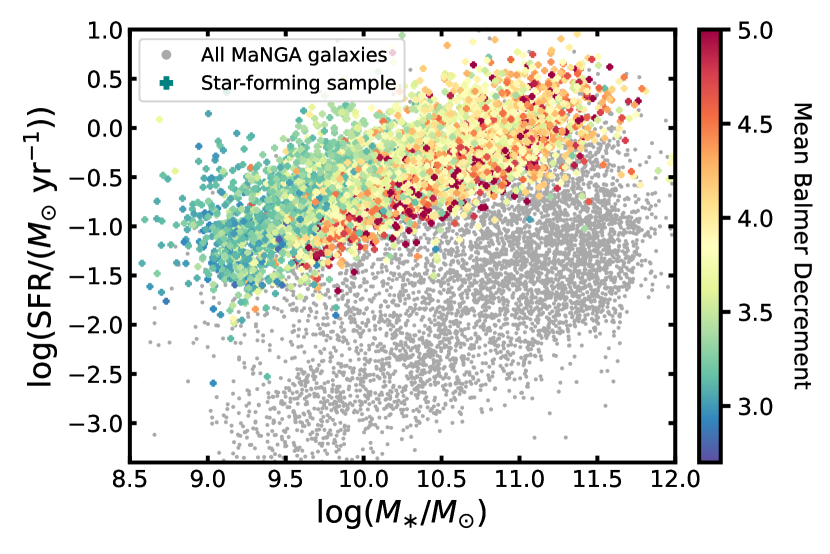
Figure 1.— Total SFR (computed from the summation of all MaNGA spaxels, without dust correction) as a function of stellar mass for the entire MaNGA DR17 galaxy sample (grey points). The 4517 star-forming galaxies used for our analysis are color-coded by the mean Balmer decrement ($f_{\rm H\alpha}/f_{\rm H\beta}$) of their star-forming spaxels meeting our selection criteria (c.f. Figure 1 of Law et al., 2021b).

III. Results

III.1. The Local Relation

Following the generic predictions of star formation feedback models (e.g., Krumholz & Burkhart, 2016; Hayward & Hopkins, 2017; Hung et al., 2019, and references therein) and results from a variety of observational studies (e.g., Green et al., 2014; Varidel et al., 2020), we expect that the MaNGA data should exhibit a positive correlation between the local gas-phase velocity dispersion in each spaxel ($\sigma_{\rm H\alpha}$) and the corresponding local star formation rate surface density ($\Sigma_{\rm SFR}$).

In Figure 2 we therefore plot $\sigma_{\rm H\alpha}$ against $\Sigma_{\rm SFR}$ for all 1.4 million spaxels in our DR17 star-forming sample, color-coded by the logarithm of the number of spaxels contributing to each location in the plot. In all cases $\sigma_{\rm H\alpha}$ for each spaxel is drawn directly from the DAP-provided data products and corrected for the instrumental LSF and a model-derived estimate of the beam smearing imparted by the MaNGA PSF (see Law et al., 2021a, their §5). $\Sigma_{\rm SFR}$ is similarly derived from the MaNGA DAP data products by converting the reported $\rm H\alpha$ flux for each spaxel to the $\rm H\alpha$ SFR following the relation defined by Kennicutt (1998, their Eqn 2):

$$\Sigma_{\rm SFR}(M_{\odot}\textrm{yr}^{-1}\textrm{kpc}^{-2})=\frac{L(\rm H\alpha)}{1.26\times 10^{41}\textrm{erg s}^{-1}}\times(0.56/\Theta)$$ (2)

where $L_{\rm H\alpha}$ in units of erg s^-1 is the dust-corrected $\rm H\alpha$ luminosity of the spaxel given the known redshift of the source, the factor of 0.56 represents a conversion to the Chabrier (2003) initial mass function from that used by Kennicutt (1998), and $\Theta$ is a scale factor representing the solid angle of a spaxel in square kpc. Our dust correction factor for each spaxel is based upon the corresponding MaNGA-observed $\rm H\alpha$/$\rm H\beta$ Balmer decrement (assuming an unreddened ratio $\rm H\alpha$/$\rm H\beta$ $=2.86$) in combination with a Cardelli et al. (1989) dust model.

Although there is substantial scatter in the measured velocity dispersion of individual spaxels (due primarily to the 2% random uncertainty in the MaNGA LSF around $\rm H\alpha$, Law et al., 2021a), there is a clear overall trend in the sense that gas-phase velocity dispersion increases across the range of star-formation rate surface densities probed by MaNGA. This trend is driven largely by the absence of spaxels at low $\sigma_{\rm H\alpha}$ and high $\Sigma_{\rm SFR}$; this absence is likely to be genuine rather than a selection bias as narrow, bright emission lines should be particularly easy to detect.

It is nonetheless difficult to get a sense of the overall trends in star-forming galaxies as an ensemble from this plot as the regions of low spaxel density confuse the impression of the statistical bulk of the spaxels which are concentrated in a narrow range around log($\Sigma_{\rm SFR}$/($M_{\odot}{\rm yr}^{-1}{\rm kpc}^{-2}$)) = -2.25 and $\sigma_{\rm H\alpha}=20-25$ km s${}^{-1}\,$ (see also Figure 3 of Law et al., 2021b). We therefore compute the $2.5\sigma$-clipped mean of the distribution in bins of $\Sigma_{\rm SFR}$, overplotting this running mean against the raw data in open black squares in Figure 2. This spaxel-averaged relation shows a clear trend, but flattens out substantially at the lowest values of $\sigma_{\rm H\alpha}$ due to the survival bias imparted by the large MaNGA LSF. That is, lower values of $\sigma_{\rm H\alpha}$ are preferentially lost from the sample as observational uncertainties scatter them below the instrumental LSF, resulting in imaginary velocity dispersions after correction for the LSF in quadrature. We explored this effect in detail in Law et al. (2021a) and provided there a series of correction factors to account for this effect as a function of both SNR and the intrinsic astrophysical velocity dispersion. Per their Figure 15, this correction can be as large as 10% at $\sigma_{\rm H\alpha}=15$ km s${}^{-1}\,$, even for SNR=100.

Table 1MaNGA Ensemble Velocity Dispersions

SFR Surface Density				SFR				SFR (1$R_{\rm e}$)
log($\Sigma_{\rm SFR}$)	$\sigma_{\rm H\alpha}$	$\epsilon_{\rm H\alpha}$		log(SFR)	$\langle\sigma_{\rm H\alpha}\rangle$	$\epsilon_{\rm H\alpha}$		log(SFR)	$\langle\sigma_{\rm H\alpha}\rangle$	$\epsilon_{\rm H\alpha}$
($M_{\odot}$ yr-1 kpc-2)	(km s${}^{-1}\,$)	(km s${}^{-1}\,$)		($M_{\odot}$ yr-1)	(km s${}^{-1}\,$)	(km s${}^{-1}\,$)		($M_{\odot}$ yr-1)	(km s${}^{-1}\,$)	(km s${}^{-1}\,$)
-2.9	17.1	7.0		-1.50	16.1	4.1		-1.70	15.5	4.2
-2.7	17.7	6.8		-1.28	15.5	3.1		-1.48	16.4	3.8
-2.5	18.8	6.7		-1.06	16.8	3.3		-1.26	17.0	3.5
-2.3	20.0	6.8		-0.84	18.3	4.0		-1.04	18.4	4.0
-2.1	21.2	6.8		-0.62	19.0	3.8		-0.82	19.1	3.8
-1.9	22.6	6.9		-0.40	20.1	4.0		-0.60	20.5	4.4
-1.7	23.9	7.0		-0.18	22.2	5.3		-0.38	22.2	5.3
-1.5	25.1	7.3		0.04	23.6	5.7		-0.16	23.6	5.2
-1.3	27.0	7.7		0.26	24.8	5.3		0.06	25.7	5.7
-1.1	29.3	8.2		0.48	26.7	5.7		0.28	28.4	6.7
-0.9	31.5	9.5		0.70	29.8	6.3		0.50	30.0	6.7
-0.7	35.8	9.1		0.92	33.0	7.2		0.72	33.5	7.2

We therefore apply a survival bias correction to the open black squares following the prescriptions of Law et al. (2021a) in order to obtain the relation given by the filled black squares in Figure 2 (see also Table 1) with error bars representing the rms width of the distribution corrected for observational uncertainties. This corrected relation is much clearer, showing that $\sigma_{\rm H\alpha}$ increases from 17 km s${}^{-1}\,$ to 35 km s${}^{-1}\,$ over about two decades in $\Sigma_{\rm SFR}$ from $10^{-2.9}$ to $10^{-0.7}$ $M_{\odot}$ yr^-1 kpc^-2. Using an unweighted least-squares fitting algorithm in log-log space, we find that this corresponds to an approximately power-law relation of the form

$$\sigma_{\rm H\alpha}=42\pm 1\left(\frac{\Sigma_{\rm SFR}}{M_{\odot}\,{\rm yr}^{-1}\,{\rm kpc}^{-2}}\right)^{0.140\pm 0.005}\rm{km\,s}^{-1}$$ (3)

Despite our focus on on spaxels outside the central 4 arcsec in each galaxy, we nonetheless note that the strength of this correlation depends at the few km s${}^{-1}\,$ level on our beam smearing correction. If we repeat the above analysis without making such a correction, we derive values that are systematically larger by 1 km s${}^{-1}\,$ at the low end of the relation and 3 km s${}^{-1}\,$ at the high end of the relation (open triangles vs open boxes in Figure 2). We return to a discussion of this effect in §IV.

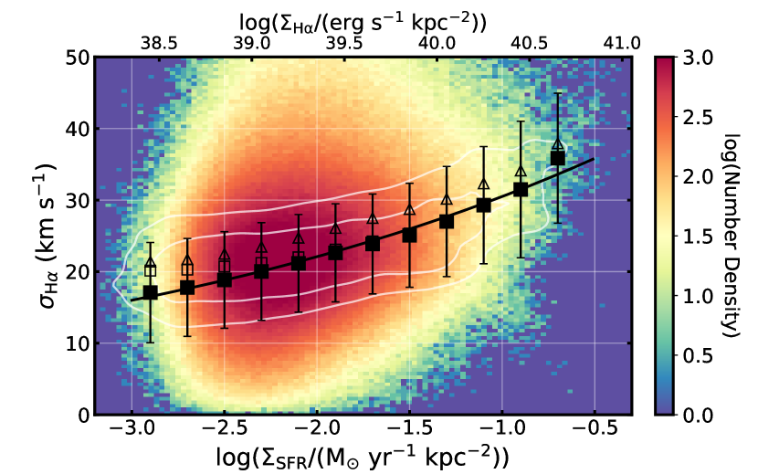
Figure 2.— Logarithmic number density plot of local $\rm H\alpha$ velocity dispersion as a function of dust-corrected star formation rate surface density and $\rm H\alpha$ surface brightness for 1.4 million spaxels from 4,517 individual galaxies in the MaNGA DR17 final data release. Grey contours represent 50% and 75% intervals in the number density distribution when counts are normalized in each bin along the $\Sigma_{\rm SFR}$ axis. Open symbols represent the moving sigma-clipped average of the distribution with (open boxes) and without (open triangles) a beam smearing correction applied to the spaxel data. Black filled squares are as the open boxes, but with an additional correction applied to account for the preferential loss of values at low $\sigma_{\rm H\alpha}$ from the distribution due to the MaNGA LSF (see discussion in text). Error bars on the black filled squares represent the $1\sigma$ width of the distribution corrected in quadrature for the expected width due to the observational uncertainties in $\sigma_{\rm H\alpha}$ and the MaNGA LSF. The black line represents a power-law fit to the relation given by Eqn. 3.

III.2. The Global Relation

In addition to presenting our results in a local sense for individual spaxels as in §III.1, it is also possible to recast our observations in terms of galaxy-averaged quantities. This approach has, for instance, been commonly adopted in studies of the high-redshift universe (e.g., Law et al., 2009; Wisnioski et al., 2015; Simons et al., 2017; Übler et al., 2019) for which a single velocity dispersion is typically quoted for each galaxy. The method of estimating that single velocity dispersion value for each galaxy can vary significantly from study to study, with some preferring to average individual measurements and others constructing physically-based models of the galaxies that can be matched to the ensemble of observed spaxels via forward modeling. Here, we follow Law et al. (2009) and Green et al. (2014) in computing the intensity-weighted mean velocity dispersion $\langle\sigma_{\rm H\alpha}\rangle$ of spaxels in each galaxy that fulfill the selection criteria defined in §II.3.

We plot this galaxy-averaged velocity dispersion in Figure 3 against two estimates of the total dust-corrected star formation rate; the total star formation rate within the MaNGA IFU footprint, and the total star formation rate within 1 effective radius of the galaxy center. The former value is computed by simply summing the $\rm H\alpha$-derived star formation rates within each galaxy data cube for all spaxels in which the nebular emission line ratios are consistent with ionization from star formation (§II.3), while the latter includes only spaxels at radii less than one $R_{\rm e}$ (given in elliptical polar coordinates by the MaNGA DAP for each galaxy). While the simple sum across the MaNGA footprint will be a closer approximation to the total galaxy SFR, the SFR within $1R_{\rm e}$ will be a more uniform statistic across the MaNGA sample, as individual galaxies can be covered out to a range of different radii along their major and minor axes.

As before, we also compute the $2.5\sigma$-clipped mean of the distribution in bins of total SFR, overplotting this running mean against the raw data in filled black squares in Figure 3 (see also Table 1) with error bars representing the rms width of the clipped distribution. No attempt has been made in this estimate to remove the observational uncertainty in individual line measurements, as such uncertainties largely average to zero in our construction of $\langle\sigma_{\rm H\alpha}\rangle$ from the individual spaxel measurements. Likewise, survival bias in the individual spaxel measurements is largely mitigated by the intensity weighting within each galaxy. For both the total SFR within the MaNGA footprint (left panel) and the total SFR within $1R_{\rm e}$ (right panel), we find that the local correlation between $\sigma_{\rm H\alpha}$ and $\Sigma_{\rm SFR}$ extends in a global sense to a strong correlation between $\langle\sigma_{\rm H\alpha}\rangle$ and the total galaxy-integrated SFR as well, increasing from 16 km s${}^{-1}\,$ to 33 km s${}^{-1}\,$ over 2.5 decades in total SFR. This relation is again well described by a power-law relation, given by

$$\langle\sigma_{\rm H\alpha}\rangle=23.6\pm 0.3\left(\frac{{\rm SFR}}{M_{\odot}\,{\rm yr}^{-1}}\right)^{0.133\pm 0.006}\rm{km\,s}^{-1}$$ (4)

As for the local relation, uncorrected beam smearing can exaggerate the strength of this correlation (open triangles in Figure 3) but does not wholly explain it.

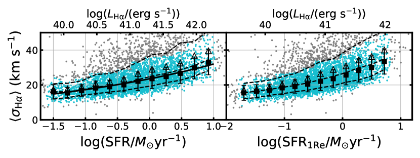
Figure 3.— Intensity averaged $\rm H\alpha$ velocity dispersion as a function of the total star formation rate in the MaNGA footprint (left panel) and within one effective elliptical radius of the galaxy center (right panel) for 4517 star-forming galaxies from MaNGA DR17 (small cyan and grey points). Black filled squares represent a moving sigma-clipped average with error bars representing the sigma-clipped rms distribution width. Grey/cyan points represent data rejected/kept by the clipping algorithm. Black open triangles represent the same quantity as the black filled squares but derived from velocity dispersions that have not been corrected for beam smearing. The solid black line represents a power-law fit to the relation given by Eqn. 4. Dashed black lines represent the 16th, 50th, and 84th percentiles of the full distribution.

We note that Figure 3 contains an appreciable number of galaxies for which $\langle\sigma_{\rm H\alpha}\rangle$ lies above the general relation with the tail of the distribution extending above the plotted range to $\sim$ 120 km s${}^{-1}\,$. Of the 4517 galaxies in this plot, 665 are effectively removed from consideration in deriving the average relation by our $2.5\sigma$ clipping algorithm: 135 have $\langle\sigma_{\rm H\alpha}\rangle>50$ km s${}^{-1}\,$, and 7 have $\langle\sigma_{\rm H\alpha}\rangle>100$ km s${}^{-1}\,$.

The physical origin of this high-dispersion tail varies significantly from galaxy to galaxy. Galaxies with $\langle\sigma_{\rm H\alpha}\rangle>50$ km s${}^{-1}\,$ are $\sim 10^{\circ}$ more highly inclined to the line of sight on average than the rest of the galaxy sample, suggesting that the line-of-sight velocity dispersion in some cases may be inflated by contributions from the rotational velocity field. In a handful of galaxies randomly selected for inspection from the high-$\langle\sigma_{\rm H\alpha}\rangle$ tail however (e.g., 7977-12701, 8332-12704) visual inspection of the galaxy spectra indicates clear multi-component nebular emission lines indicative of bulk gas flows that cannot be well fit by the single-component gaussian models used by the DAP. We defer treatment of such multi-component profiles to future work, and simply note here that they represent a small fraction of the overall MaNGA galaxy sample.

III.3. Comparison to Recent Literature

While the MaNGA relation between $\sigma_{\rm H\alpha}$ and star formation rate shown in Figures 2 and 3 represents by far the largest sample of galaxies from across the entire star forming main sequence to date, our results largely confirm previous measurements made from smaller galaxy samples (often made at much higher spectral resolution). Forty years ago for instance, Terlevich & Melnick (1981) measured gas-phase velocity dispersions for a selection of extragalactic HII regions, finding typical $\sigma_{\rm H\alpha}=15-30$ km s${}^{-1}\,$ in excellent agreement with the values that we have derived from the overall star forming galaxy population. In Figure 4 we compare our observed MaNGA relations between $\sigma_{\rm H\alpha}$, the local star formation rate surface density, and the total galactic star formation rate against a variety of other studies from the recent literature.

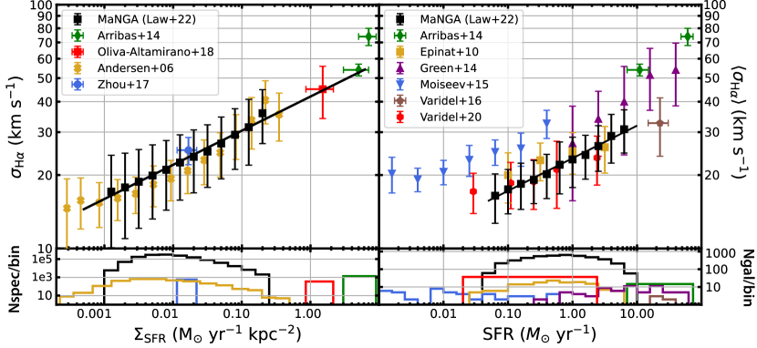
Figure 4.— Per-spaxel velocity dispersion $\sigma_{\rm H\alpha}$ as a function of the local star formation rate surface density $\Sigma_{\rm SFR}$ (left panel) and galaxy-averaged $\langle\sigma_{\rm H\alpha}\rangle$ as a function of the galaxy-integrated star formation rate (right panel) for MaNGA DR17 galaxies and other $z=0$ samples from the literature. Star formation rates for all samples are consistently shown dust-corrected using a Chabrier (2003) IMF. As in Figures 2 and 3 the MaNGA data points represent moving averages computed for 4517 MaNGA galaxies with error bars showing the clipped $1\sigma$ range of the distribution after correction for the additional scatter introduced by the uncertainty in the LSF. Literature values are similarly averaged across individual galaxies with error bars showing the range of the distribution, including 32/16 LIRGs/ULIRGs from Arribas et al. (2014), 7 star forming galaxies from Zhou et al. (2017), 7 DYNAMO galaxies with 400 pc adaptive-optics resolution observations from Oliva-Altamirano et al. (2018), 59 dwarf galaxies from Moiseev et al. (2015), 39 spiral galaxies from Andersen et al. (2006), 153 galaxies from Epinat et al. (2010), six starburst galaxies from Varidel et al. (2016), 67 starburst galaxies from Green et al. (2014), and 383 galaxies from the combined SAMI+DYNAMO sample (Varidel et al., 2020). The histograms in the lower panels show the logarithmic number of spectra (left-hand panel) or galaxies (right-hand panel) contributing to each bin in SFR or $\Sigma_{\rm SFR}$ for each of the different samples (assuming 100 spectra per galaxy for the Arribas et al. (2014), Oliva-Altamirano et al. (2018), and Zhou et al. (2017) samples).

Andersen et al. (2006) for instance found an average $\sigma_{\rm H\alpha}=18\pm 4$ km s${}^{-1}\,$ (see their Figure 6) from DensePak IFU (Barden et al., 1998) echelle spectroscopy of 39 face-on spirals (mean inclination 23^∘) with a comparable spatial resolution to MaNGA ($\sim 1.1$ kpc median fiber diameter). This agrees well with the low-$\Sigma_{\rm SFR}$ end of the MaNGA distribution where the peak number of spaxels are located for both the MaNGA and the DensePak data (Figure 4, lower panels). Reprocessing the DensePak line-width data from Andersen et al. (2006) with the flux calibration from Andersen et al. (2013) to present the results as a function of $\Sigma_{\rm SFR}$ (Figure 4, gold points in left-hand plot) we find excellent agreement in the trend of increasing $\sigma_{\rm H\alpha}$ with increasing $\Sigma_{\rm SFR}$ as well. We select only DensePak spectra consistent with star-forming regions using $\rm\log[NII]\lambda 6584/H\alpha<-0.3$ based on [NII] line-fluxes from D. Andersen (private comm.); this is a conservative selection in the context of Equation 1. We have applied Equation 2 with a variable dust correction factor assuming that the Balmer decrement varies from 2.86 to 4.5 as a function of the $\rm H\alpha$ surface brightness in a manner similar to that observed in the MaNGA spaxel sample (see Figure 5). While no correction for beam-smearing has been applied, the line-widths have been corrected for the instrumental broadening. The DensePak and MaNGA relations are in excellent agreement to within observational uncertainty, despite the DensePak data having substantially higher spectral resolution $R\sim 13,000$ providing an instrumental $1\sigma$ LSF of just 10 km s${}^{-1}\,$.

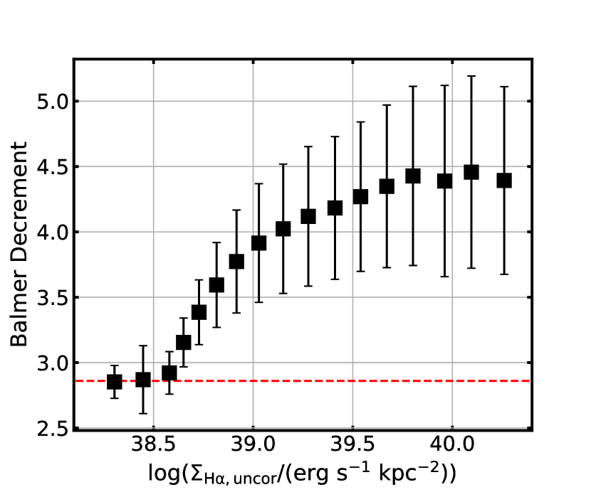
Figure 5.— Average Balmer decrement (i.e., $\rm H\alpha$/$\rm H\beta$) measured from the MaNGA spaxel data in Figure 2 as a function of the uncorrected $\rm H\alpha$ surface brightness $\Sigma_{\rm\rm H\alpha,uncor}$. Error bars indicate the $1\sigma$ width of the spaxel distribution. The dashed red line represents the constant value of 2.86 corresponding to the nominal dust-free value under Case B recombination (Osterbrock & Ferland, 2006).

Similarly, Epinat et al. (2008, 2010) presented Fabry-Perot $\rm H\alpha$ kinematics for a sample of $\sim 100$ nearby spiral galaxies from the GHASP survey and found average $\rm H\alpha$ velocity dispersion $\langle\sigma_{\rm H\alpha}\rangle=24\pm 5$ km s${}^{-1}\,$. Binning the results from their online supplemental data according to SFR (and applying a dust correction factor of 2.0 based on the average correction for the MaNGA star forming galaxy sample), we find a relation that matches the MaNGA data to within an average of 1.2 km s${}^{-1}\,$.

More recently, observations from the SAMI IFU survey have also been used to assess the velocity dispersion of galactic disks. Zhou et al. (2017) for instance analyzed SAMI velocity maps for 8 local star forming galaxies and found $\sigma_{\rm H\alpha}$ in the range 20-30 km s${}^{-1}\,$ for galaxies with $\Sigma_{\rm SFR}\approx 10^{-2}M_{\odot}$ yr^-1 kpc^-2, in excellent agreement with our results (Figure 4, left-hand panel). Likewise, Varidel et al. (2020) analyzed a sample of 383 galaxies from the combined SAMI and DYNAMO samples and found a statistically significant correlation between SFR and $\langle\sigma_{\rm H\alpha}\rangle$. As indicated by Figure 4 (right-hand panel), in the SFR range of overlap between the MaNGA and SAMI samples the MaNGA velocity dispersions are larger on average by about 0.4 km s${}^{-1}\,$, consistent with the 0.7 km s${}^{-1}\,$ that we found in Law et al. (2021a, see their Figure 21) for a sample of galaxies observed in common between the two surveys. We note, however, that Varidel et al. (2020) made an inclination-dependent correction to their observations and thus estimate the vertical disk velocity dispersion $\sigma_{\rm z}$ rather than the simple line-of-sight velocity dispersion. As discussed in §V, if we were to make such a correction our results would shift downward by $\sim 1.5$ km s${}^{-1}\,$, and nonetheless still be a reasonable match to within 1.1 km s${}^{-1}\,$. Broadly speaking, the MaNGA and SAMI data thus give much the same trend, with the higher spectral resolution SAMI data complemented by the 10x larger MaNGA sample.

At lower star formation rates, Moiseev et al. (2015) used scanning Fabry-Perot interferometry to study the ionized gas in 59 nearby dwarf galaxies (SFR 0.001 to 0.1 $M_{\odot}$ yr^-1). While these authors observed a trend between $\langle\sigma_{\rm H\alpha}\rangle$ and SFR similar to ours, this trend appears offset relative to the MaNGA, GHASP, and SAMI observations. Adding a 3 km s${}^{-1}\,$ natural line width and 9 km s${}^{-1}\,$ thermal broadening back into their data in quadrature for consistency with our observations (since these authors subtracted these quantities from their published values), we note that their 20-30 km s${}^{-1}\,$ values are systematically about 10 km s${}^{-1}\,$ higher than the MaNGA observations at similar SFR. The reason for this discrepancy is unclear; while it may reflect a genuine difference between the dwarf galaxy population and the star forming main sequence at higher stellar masses, it may also be due in part to systematic differences between the survey analysis techniques.

At higher star formation rates, Green et al. (2014) (see also Green et al., 2010) presented initial results from the DYNAMO survey of 67 $z\sim 0.1$ starburst galaxies (SFR $0.2-57M_{\odot}$/yr). While these authors found a similar correlation between $\sigma_{\rm H\alpha}$ and total SFR, their relation is steeper than ours, reaching $40-50$ km s${}^{-1}\,$at $10M_{\odot}$ yr^-1 instead of 30 km s${}^{-1}\,$. Arribas et al. (2014) and García-Marín et al. (2009) likewise observed large values of $\sigma_{\rm H\alpha}$ for a sample of 58 LIRGs and ULIRGs, as did Varidel et al. (2016) for six $z<0.04$ starburst galaxies observed with the WiFeS IFU, and Oliva-Altamirano et al. (2018) for Keck/OSIRIS IFU observations (at 400 pc adaptive-optics resolution) for a sample of 7 disk galaxies reobserved from the DYNAMO sample. As illustrated in Figure 4 (left-hand panel), the Arribas et al. (2014) and Oliva-Altamirano et al. (2018) samples represent SFR surface densities 1-1.5 orders of magnitude larger than those probed by the MaNGA sample, yet nonetheless the LIRG and DYNAMO samples agree fairly well with our extrapolated $\sigma_{\rm H\alpha}-\Sigma_{\rm SFR}$ relation (though the 70 km s${}^{-1}\,$ ULIRG sample is still notably high). In terms of total SFR the Varidel et al. (2016) sample (using their flux-weighted mean $\sigma_{\rm H\alpha}$ corrected for beam smearing) agrees well with the extrapolated MaNGA relation, while the Arribas et al. (2014) LIRG/ULIRG data points are both substantially higher.

Finally, we note that an early analysis of the MaNGA data was presented by Yu et al. (2019), who used 648 galaxies from the MaNGA MPL-5 (DR14) data set and similarly noted positive correlations between velocity dispersion and SFR, $M_{\ast}$, and $\Sigma_{\rm SFR}$. However, this study had significantly different methodology than our present contribution. First, Yu et al. (2019) measured the $\rm H\alpha$ velocity dispersion from stacked galaxy spectra, which included a substantial component due to galactic rotation (although this was partially mitigated by their beam smearing correction and preferential selection of face-on spiral disks). Second, as demonstrated in Law et al. (2021a) the DR14 data products used by Yu et al. (2019) adopted an instrumental LSF estimate that was in error by about 5% in the vicinity of $\rm H\alpha$. As a result, the 30-50 km s${}^{-1}\,$ values presented by Yu et al. (2019) were likely systematically overestimated by about 15 km s${}^{-1}\,$ compared to the DR17 analysis of the full MaNGA data set presented here.

IV. Secondary Relations

In §III we confirmed the existence of a correlation between gas-phase velocity dispersion and both the local star formation rate surface density and the galaxy-integrated total star formation rate, as expected on the basis of theoretical work and recent observational studies. However, there are multiple other correlations that can be physically expected as well; for instance, since the most rapidly star forming galaxies on the main sequence tend to be the most massive, we would expect to see a correlation between velocity dispersion and stellar mass as well. Likewise, artifacts produced by an imperfect beam smearing correction would tend to be largest for the highest mass galaxies, potentially masquerading as a correlation with the star formation rate. In this section, we use the statistical power of MaNGA to investigate such correlations and narrow down the most likely physical cause of the enhanced velocity dispersions.

IV.1. Redshift

The redshift range of the MaNGA sample ($z=0.015-0.1$) is too small to expect any significant physical evolution in the galaxy population, and therefore presents a good test of our ability to separate genuine physical trends in $\langle\sigma_{\rm H\alpha}\rangle$ from trends imparted by the correlation of $z$ with other observables. Specifically, redshift is strongly correlated with both stellar mass and total SFR (see, e.g., Law et al., 2021b, their Figure 1) for the simple reason that massive, high-SFR disk galaxies are rare and thus occur more frequently at larger redshifts corresponding to a larger survey volume. At the same time, our fixed angular resolution will correspond to larger physical scales at higher redshifts, resulting in more significant beam smearing.

Both effects will tend to produce a relation in the sense that we expect $\langle\sigma_{\rm H\alpha}\rangle$ to increase as a function of redshift. Indeed, this is exactly what we see in Figure 6 (left panel, dashed black line). However, this apparent relation is driven by the correlation of $z$ with total SFR; if we subdivide the sample into bins by SFR (Fig. 6, left panel, colored lines) we note that there is no relation between $\langle\sigma_{\rm H\alpha}\rangle$ and $z$ within a given SFR bin. In contrast, $\langle\sigma_{\rm H\alpha}\rangle$ increases consistently between each bin in SFR, and the dominance of high-SFR galaxies at high-z produced the apparent relation.

Figure 6 also provides a sanity check on our beam smearing correction; if there were a significant uncorrected effect from beam smearing we should expect these relations to increase as a function of $z$ even within a given SFR bin, which is exactly what we see if we use values of $\langle\sigma_{\rm H\alpha}\rangle$ that have not been corrected for beam smearing (right-hand panel).

Figure 6.— Galaxy-averaged $\rm H\alpha$ velocity dispersion with (left panel) and without (right panel) beam smearing correction applied as a function of redshift for all star-forming galaxies (dashed black line and points) and for four bins in the total star formation rate (colored lines and points). All points represent $2.5\sigma$-clipped means applied to the observational sample. Statistical uncertainties in the mean for each point are $<1$ km s${}^{-1}\,$. The apparent relation between $\langle\sigma_{\rm H\alpha}\rangle$ and redshift after beam-smearing correction is driven by the strong relation between redshift and total SFR.

IV.2. Stellar Mass

By definition, the star-forming galaxy main sequence describes a correlation between stellar mass and star-formation rate, and the intensity averaged gas-phase velocity dispersion $\langle\sigma_{\rm H\alpha}\rangle$ is strongly correlated with the position of a galaxy along this sequence. As illustrated in Figure 7 (top panel), the lowest velocity dispersions $\langle\sigma_{\rm H\alpha}\rangle\sim 15$ km s${}^{-1}\,$ occur at the lower end of this sequence, while the highest values $\sim 40$ km s${}^{-1}\,$ occur at the upper end of the sequence. However, to what extent is the increase due to the increasing stellar mass (increasing both the gravitational potential of the galactic disk and the magnitude of shear within that disk) vs the increasing star formation rate (increasing the amount of feedback injected into the interstellar medium)? Is it possible to distinguish which is the primary correlation, and which is simply a secondary correlation?

We endeavour to break this degeneracy by subdividing the galaxy sample according to quartiles in both SFR and stellar mass, and plotting the residual correlations within each quartile.

In Figure 7 (lower-left panel) we show the $2.5\sigma$-clipped mean $\langle\sigma_{\rm H\alpha}\rangle$ as a function of stellar mass for the overall galaxy sample (dashed black line), and for four quartiles in the total SFR (colored lines). We note that the overall relation for all galaxies considered together shows a strong positive correlation, and runs between 17 km s${}^{-1}\,$ and 25 km s${}^{-1}\,$. Within individual quartiles in total SFR however, this correlation with stellar mass is almost entirely absent. While the lowest-SFR bin (filled circles) increases slightly from 17 - 20 km s${}^{-1}\,$ with increasing stellar mass, the second (downward-pointing triangles), third (upward-pointing triangles), and fourth (diamonds) quartiles in SFR show no such increase (and if anything mild evidence for a decrease) in $\sigma_{\rm H\alpha}$ with increasing $M_{\ast}$.

If galaxies were homologous systems, which is generally a good first order approximation when studying galaxy scaling relations, and the $\langle\sigma_{\rm H\alpha}\rangle$ was tracing the gravitational potential, one would expect a $\langle\sigma_{\rm H\alpha}\rangle\propto\sqrt{M_{\ast}}$ dependence. This implies that if $\langle\sigma_{\rm H\alpha}\rangle=25$ km s${}^{-1}\,$ at $10^{11}M_{\odot}$ one would expect $\langle\sigma_{\rm H\alpha}\rangle=25/\sqrt{10}=8$ km s${}^{-1}\,$ at $10^{10}M_{\odot}$; even the overall global trend is clearly much more shallow than this.

In contrast, in Figure 7 (lower-right panel) we show the $2.5\sigma$-clipped mean $\langle\sigma_{\rm H\alpha}\rangle$ as a function of SFR for the overall galaxy sample (dashed black line), and for four quartiles in the total stellar mass (colored lines). This overall relation is stronger than the $\langle\sigma_{\rm H\alpha}\rangle$ - $M_{\ast}$ relation, running between 15 km s${}^{-1}\,$ and 30 km s${}^{-1}\,$. In addition, the correlation between $\langle\sigma_{\rm H\alpha}\rangle$ and SFR very closely follows the average relation in all four of the mass-quartile bins with no evidence of a systematic vertical offset between the bins.

Figure 7.— Top panel: Total stellar mass (derived from the NSA catalog, Blanton et al., 2011) vs total extinction-corrected $\rm H\alpha$ star formation rate within the MaNGA footprint for all 4517 galaxies in our star-forming sample, color-coded by their intensity-averaged $\rm H\alpha$ velocity dispersion. Solid black lines show the corresponding quartile divisions in both axes, the dashed black line shows a power-law fit to the MaNGA main sequence using an orthogonal distance regression algorithm. $\langle\sigma_{\rm H\alpha}\rangle$ is strongly correlated with location along this star-forming main sequence. Bottom-left panel: $\langle\sigma_{\rm H\alpha}\rangle$ as a function of stellar mass for all points (dashed black line) and for four quartiles in SFR (colored lines). Bottom-right panel: $\langle\sigma_{\rm H\alpha}\rangle$ as a function of SFR for all points (dashed black line) and for four quartiles in stellar mass (colored lines). All points represent $2.5\sigma$-clipped means applied to the observational data.

We therefore conclude that the correlation between $\langle\sigma_{\rm H\alpha}\rangle$ and SFR is the primary relation, and that the apparent correlation with stellar mass is driven by the preferential location of high-SFR objects at higher stellar masses.

Numerous authors have similarly examined the relation between $\langle\sigma_{\rm H\alpha}\rangle$ and stellar mass in the past, with mixed results. Moiseev et al. (2015) for instance concluded that the trend of $\langle\sigma_{\rm H\alpha}\rangle$ was stronger with $\rm H\alpha$ luminosity than with stellar mass for their sample of dwarf galaxies, as did Varidel et al. (2020) for the SAMI galaxy sample. Unlike Varidel et al. (2020) however, we do not see evidence of a residual correlation between $\langle\sigma_{\rm H\alpha}\rangle$ and $M_{\ast}$ after accounting for the SFR relation. Epinat et al. (2010) did not observe a correlation between $\langle\sigma_{\rm H\alpha}\rangle$ and the maximum rotation velocity (i.e., a proxy for stellar mass) of galaxies in their sample, but noted that at higher redshifts (or lower spatial resolution) beam smearing was capable of artificially producing such a trend if uncorrected. The importance of beam smearing matches with our own observations; our $\langle\sigma_{\rm H\alpha}\rangle$ vs stellar mass relation is nearly twice as strong if we were to instead use velocity dispersions that have not been corrected for beam smearing, and less straightforward to disentangle from the SFR relation. Given how shallow the beam-smearing corrected trend with stellar mass is in the MaNGA data, Monte Carlo tests drawing random subsamples of our data suggest that it is unsurprising that Epinat et al. (2010) would have been unable to detect it in a sample 1/40th the size of MaNGA.

IV.3. Specific SFR, Main Sequence Offset, and Gas Fraction

Similarly to §IV.2, we can investigate whether any other variations on the SFR are even more closely correlated to the ionized gas velocity dispersion. Following Varidel et al. (2020), we compute both the specific star formation rate (SSFR, i.e. the total SFR divided by the stellar mass) and the main-sequence SFR offset ($\Delta$MS, i.e. the SFR ‘excess’ of a given galaxy above the MaNGA-derived main sequence mean for the stellar mass; see dashed line in Figure 7). As indicated by Figure 8 we see correlations of $\langle\sigma_{\rm H\alpha}\rangle$ with both quantities. However, these trends appear to again be be driven primarily by the underlying correlation with total SFR as suggested by the vertical offset in the colored lines. While there appears to be a residual trend within the highest-SFR bin, this is an artifact of the wide range of this bin and disappears if we subdivide further in total SFR (see, e.g., §IV.4).

Figure 8.— Intensity-weighted mean $\rm H\alpha$ velocity dispersion for galaxies in the MaNGA sample as a function of their specific star formation rate (left-hand panel), SFR offset from the main sequence (middle panel), and HI gas fraction (right-hand panel). HI gas fractions are based on 1732 galaxies of the sample with HI gas masses drawn from Stark et al. (2021). The majority of the trends in all panels are best explained by the vertical offset between individual quartiles of the galaxy sample in total SFR (colored lines and points). All points represent $2.5\sigma$-clipped means applied to the observational data.

Additionally, we compute the HI gas fraction using Green Bank Telescope and ALFALFA HI masses drawn from the ongoing HI-MaNGA survey (Masters et al., 2019; Stark et al., 2021). We find that 1732 of our galaxies have HI measurements flagged as reliable in v2.0.1 of the HI-MaNGA catalog. In Figure 8 (right-hand panel) we show the intensity-weighted velocity dispersion as a function of the HI gas fraction, and observe a small decline of $\sim 3-4$ km s${}^{-1}\,$ from 0-60% gas fraction that is statistically significant at $8\sigma$ based on the error in the mean. Varidel et al. (2020) noted a similar relation in their SAMI data, although these authors were unable to determine if the relation was significant. This relation, however, appears to be a consequence of the anticorrelation between gas fraction and total SFR in the sense that the largest gas fractions occur in the lowest mass galaxies with low total SFR. As indicated by the colored lines in Figure 8 (right-hand panel), no such trends are convincing within individual SFR bins.

IV.4. SFR Surface Density

Finally, we investigate whether we can break the correlation between local star formation rate surface density $\Sigma_{\rm SFR}$ and the total galaxy-integrated SFR in order to determine whether local or global properties are the physical driver of the observed relation. The underlying tension between local and global galaxy properties and their respective influence on star formation has been a subject of substantial debate for many years (see, e.g., Sánchez et al., 2021a, b, and references therein for a recent review).

Unsurprisingly, as indicated by Figure 9 $\Sigma_{\rm SFR}$ and total SFR are closely correlated with each other in the sense that the regions of highest SFR surface density ($\Sigma_{\rm SFR}\sim 10^{-1.5}M_{\odot}$ yr^-1 kpc^-2) tend to live within the most rapidly star-forming galaxies. There is nonetheless a wide range though, with regions of $\Sigma_{\rm SFR}=10^{-2.5}M_{\odot}$ yr^-1 kpc^-2 occurring in galaxies of all SFR. Thus, it should be possible to test whether the velocity dispersion is higher near regions of active star formation in lower-SFR galaxies or far away from regions of active star formation in higher-SFR galaxies.

Figure 9 demonstrates the results relatively convincingly on its own; the sigma-clipped mean $\sigma_{\rm H\alpha}$ as a function of location within the diagram increases strongly with SFR, but less convincingly with $\Sigma_{\rm SFR}$. We dissect this furter in Figure 10, breaking the relation between $\Sigma_{\rm SFR}$ and $\sigma_{\rm H\alpha}$ into multiple bins of total SFR, with Table 2 giving the translation of percentile ranges from the MaNGA sample to actual SFR. We observe that this relation appears to be governed primarily by the correlation between $\Sigma_{\rm SFR}$ and total SFR; at fixed $\Sigma_{\rm SFR}$ there is a strong increase in $\sigma_{\rm H\alpha}$ as a function of total SFR (from 17-30 km s${}^{-1}\,$ at $\Sigma_{\rm SFR}=10^{-2}M_{\odot}$ yr^-1 kpc^-2). In contrast, $\sigma_{\rm H\alpha}$ is nearly constant over two orders of magnitude as a function of $\Sigma_{\rm SFR}$ at fixed SFR.

Although there may be a small positive relation with $\Sigma_{\rm SFR}$ in higher-SFR bins (visible also as slight vertical gradients in $\sigma_{\rm H\alpha}$ in Figure 9), the majority of such trends are produced by residual correlations between $\Sigma_{\rm SFR}$ and SFR within each SFR bin. If, for instance, we had plotted a single bin of galaxies with SFR between the 75th and 100th percentiles we would have observed a strong correlation between $\Sigma_{\rm SFR}$ and $\sigma_{\rm H\alpha}$. Splitting this out as we have done into 75th-90th percentile, 90th-95th percentile, etc. we see that the trend is driven more by the total SFR.

We therefore conclude that the increase of ionized gas velocity dispersion is driven more by the global SFR of a galactic disk than by local properties governing the injection of supernova feedback at the sites of peak star formation within that disk. We caution, however, that the SFR itself is likely not the underlying physical driver of the observed relation, and some other as-yet untested global quantity that correlates strongly with total SFR (e.g., the total molecular gas mass) may be the true cause.

One potential explanation for this may be that (at least at kpc scales) velocity dispersions are set largely by the global increase of the disk midplane pressure in the presence of larger quantities of cold gas, and correspondingly higher star formation rates. Indeed, both Hughes et al. (2013) and Sun et al. (2020) noted that giant molecular clouds appear to ‘know’ about the global properties of their host galaxies, with galaxies with higher stellar masses and SFR hosting molecular gas with higher surface densities and velocity dispersions. As we demonstrate in §VI.2, after accounting for physics internal to HII regions the velocity dispersion of the molecular gas disk in which HII regions are embedded increases with total molecular gas mass density in agreement with recent ALMA CO (2-1) observations. While localized phenomena such as spiral arms and bars tend to be associated with regions of enhanced velocity dispersion as well both in molecular gas observations (e.g., Sun et al., 2020) and in theoretical models (e.g., Nguyen et al., 2018), these effects may simply be difficult to discern at the dynamic range and kpc-scale resolutions to which MaNGA is sensitive (although see discussion in §V).

Our results therefore take a step towards understanding why some studies have found a relation between $\Sigma_{\rm SFR}$ and $\sigma_{\rm H\alpha}$ at higher redshifts (e.g., Swinbank et al., 2012; Lehnert et al., 2013) while others have not (e.g., Übler et al., 2019, their Fig 8). With low number statistics and coarse spatial resolution, the strength of this relation will be driven in large part by the range and distribution of SFR in the galaxy sample instead of the dynamic range of the observations within any individual galaxy. Likewise, the findings from Colina et al. (2005) and Arribas et al. (2014) that localized peaks in velocity dispersion don’t tend to be correlated with peaks in $\Sigma_{\rm SFR}$ in local LIRGs/ULIRGs are naturally explained if $\Sigma_{\rm SFR}$ is not the primary driver of enhanced velocity dispersions.

Table 2SFR Percentiles

Percentile	log(SFR/$M_{\odot}$ yr-1)
0%	-2.02
25%	-0.61
50%	-0.20
75%	0.19
90%	0.51
95%	0.70
98%	0.90
100%	2.09

Figure 9.— Local star-formation rate surface density $\Sigma_{\rm SFR}$ for individual MaNGA spaxels vs the total SFR of the galaxy within which they reside, color-coded by the $2.5\sigma$-clipped mean $\rm H\alpha$ velocity dispersion of the spaxels at each point. Solid white contours indicate the linear number density distribution of spaxels within the plot. Binning artifacts in the SFR axis are caused by the discrete nature of the integrated SFR for the 4517 galaxies in the MaNGA sample compared to the 1.4 million individual spaxel measurements. High-$\Sigma_{\rm SFR}$ spaxels are located almost exclusively in high-SFR galaxies.

Figure 10.— Spaxel velocity dispersion as a function of the local star formation rate surface density $\Sigma_{\rm SFR}$ for a variety of bins in total galaxy SFR (colored points and lines). The mean relation for all galaxies (dashed black line; see Figure 2) is produced primarily by the offset between individual SFR subsamples, which are nearly flat as a function of $\Sigma_{\rm SFR}$. Individual points represent $2.5\sigma$-clipped averages of the observational data.

V. Disk Inclination and Azimuthal Angle

Thus far, we have made no explicit cuts to the galaxy sample in terms of the inclination $i$ of the galactic disk to the line of sight, nor any corrections for inclination-dependent effects. Indeed, the full MaNGA galaxy sample was selected in a manner agnostic to inclination, although there is a small bias towards more face-on galaxies ($i=0^{\circ}$) at a given stellar mass because additional extinction in edge-on disks ($i=90^{\circ}$) tends to give fainter optical magnitudes corresponding to a smaller redshift volume (see discussion by Wake et al., 2017). As such, MaNGA galaxies span a wide range of inclinations from $i=0^{\circ}-90^{\circ}$ with mean and median values of 56^∘ and 57^∘ respectively, consistent with expectations for a population of randomly-oriented disks ($57.3^{\circ}$ and $60^{\circ}$ respectively; see derivation in Appendix A of Law et al., 2009).

Here, we have estimated the inclination of our star-forming disk sample based on the $r$-band Sersic profile morphological minor and major axis lengths given by the NSA catalog (Blanton et al., 2011) from which the MaNGA parent catalog was derived. Assuming an intrinsic axis ratio of $q_{0}=0.15$ (e.g. Ryden, 2006), the inclination is given by (Holmberg, 1958):

$$\textrm{cos}^{2}i=\frac{(b/a)^{2}-q_{0}^{2}}{1-q_{0}^{2}}$$ (5)

where $a$ and $b$ are the major and minor axis lengths respectively.

In the past, many studies have opted to focus on face-on disk galaxies in order to ensure that the the observed line-of-sight velocity dispersion $\sigma_{\rm los}$ is nearly the disk vertical velocity dispersion ($\sigma_{\rm z}$) and minimize confusion from the radial ($\sigma_{\rm r}$) and azimuthal ($\sigma_{\phi}$) components, along with minimizing observational biases from beam smearing that are more severe at large inclinations (see, e.g., Cappellari, 2020). Using the statistical power of the MaNGA sample, we quantify the magnitude of such effects at kpc-scale resolution for the star-forming main sequence galaxy distribution at $z=0$.

Figure 11.— Top panels: Line-of-sight velocity dispersion $\sigma_{\rm los}$ (defined equal to the observed $\sigma_{\rm H\alpha}$) as a function of galaxy inclination $i$ and spaxel azimuthal angle $\phi$ for various ranges of both (solid black and colored lines respectively). $i=0^{\circ}/90^{\circ}$ corresponds to face-on/edge-on systems respectively, while $\phi=0^{\circ}/90^{\circ}$ corresponds to locations on the major/minor axis respectively. Dashed grey lines indicate the expected value of $\sigma_{\rm H\alpha}$ given by Equation 7 with the best-fit choices for $\sigma_{z}/\sigma_{r}$ and $\sigma_{\phi}/\sigma_{r}$; the turnover in this relation in the top-left panel is due to the preferential bias of MaNGA spaxels towards the major axis for the most edge-on galaxies. Bottom panels: Disk vertical velocity dispersion $\sigma_{z}$ as a function of galaxy inclination $i$ and spaxel azimuthal angle $\phi$ for an appropriate choice of $\sigma_{z}=0.85\sigma_{r}$ and $\sigma_{\phi}=0.91\sigma_{r}$. All points represent $2.5\sigma$-clipped means applied to the observational data.

In Figure 11 (top panels) we plot our observed $\sigma_{\rm H\alpha}\equiv\sigma_{\rm los}$ as a function of both the galaxy inclination angle $i$ and the disk azimuth angle $\phi$ of each spaxel (where the values reported by the DAP have been collapsed via symmetry to the range $\phi=0^{\circ}-90^{\circ}$, such that $\phi=0^{\circ}$ and $\phi=90^{\circ}$ correspond to the disk major and minor axes respectively, as given by the NSA catalog). In each plot, we further subdivide the points according to bins in the other parameters; i.e., we plot $\sigma_{\rm H\alpha}$ as a function of $i$ for various bins in $\phi$, and as a function of $\phi$ for various bins in $i$.

We note that the overall $\sigma_{\rm H\alpha}$ increases by about 3 km s${}^{-1}\,$ as a function of $i$ for all $\phi$, albeit slightly offset from each other. Likewise, $\sigma_{\rm H\alpha}$ increases by about 1 km s${}^{-1}\,$ as a function of $\phi$ overall, with both a difference in slope and a vertical offset for different ranges in $i$.

At the most simplistic level, we assess the potential bias that these trends have on our derived relation between $\langle\sigma_{\rm H\alpha}\rangle$ and SFR by plotting the relation for sub-populations of inclination and azimuthal angle in Figure 12. As expected from the relative amplitude of the trends with $i$ and $\phi$, such effects represent only a minor perturbation to the overall relation.

Figure 12.— Intensity-weighted mean velocity dispersion as a function of total dust-corrected star formation rate for the entire galaxy sample (black line, c.f. Figure 3) and for subsamples in galaxy inclination $i$ and spaxel azimuthal angle $\phi$ (colored lines). Although inclination of the galaxy sample shifts the overall trend slightly, it is nonetheless strong in all subsamples. All points represent $2.5\sigma$-clipped means applied to the observational data.

However, we can also go a step further by noting that changes in $\sigma_{\rm H\alpha}$ are produced by the inclusion of radial ($\sigma_{r}$) and azimuthal ($\sigma_{\phi}$) velocity dispersions into the line of sight projected velocity dispersion that was dominated by the disk vertical velocity dispersion $\sigma_{\rm z}$ for face-on galaxies. Both radial and azimuthal components increase in importance as $i$ increases; for larger inclinations $\sigma_{\phi}$ becomes dominant on the major axis ($\phi<30^{\circ}$) while $\sigma_{r}$ becomes dominant on the minor axis ($\phi>60^{\circ}$).

Mathematically, for a cylindrical alignment of the velocity ellipsoid (which is appropriate in the disk plane) the combination of these effects is given by geometric projection (see, e.g. Cappellari, 2020, their Eqn. 27) as:

$$\sigma_{\rm los}^{2}=\left(\sigma_{r}^{2}{\rm sin}^{2}\phi+\sigma_{\phi}^{2}{\rm cos}^{2}\phi\right){\rm sin}^{2}i+\sigma_{z}^{2}{\rm cos}^{2}i$$ (6)

Following (Martinsson et al., 2013, their Eqn. 10), we define $\alpha=\sigma_{z}/\sigma_{r}$ and $\beta=\sigma_{\phi}/\sigma_{r}$, in which case Equation 6 can be rearranged as

$$\sigma_{z}^{2}=\frac{\sigma_{\rm los}^{2}}{{\rm cos}^{2}i}\left[1+\frac{{\rm tan}^{2}i}{\alpha^{2}}({\rm sin}^{2}\phi+\beta^{2}{\rm cos}^{2}\phi)\right]^{-1}$$ (7)

Making the approximate assumption of axisymmetry, which is appropriate for spiral galaxies, the intrinsic components of the velocity ellipsoid $\sigma_{z}$, $\sigma_{r}$, $\sigma_{\phi}$ (or equivalently, $\sigma_{z}$, $\alpha$, and $\beta$) must be constant at a given galactocentric radius in the disk plane. If one further assumes that the gas kinematics of the galaxy population shares the same anisotropy $\alpha$ and $\beta$, one can use the variations of the projected $\sigma_{\rm los}$ at different inclinations and azimuthal angles to measure $\alpha$ and $\beta$ from the data. Here we determine these parameters by trying to remove any dependency of $\sigma_{z}$ on both inclination and azimuth angle.

We approach this problem numerically by considering a grid of $\alpha$, $\beta$ in the range $0.6-1.1$ sampled every $0.01$ dex; for each grid point we compute the slope of $\sigma_{z}$ as a linear function of $i$ and of $\phi$, and sum the absolute values of these two slopes to compute a ‘flatness’ statistic $\Omega$, the uncertainty of which is given by the quadratic sum of the uncertainties in each of the two slopes. In Figure 13 we show this surface in $\Omega$ and note that there is a well-defined global minimum at

$$\sigma_{z}/\sigma_{r}=0.84\pm{0.03}$$ (8)

and

$$\sigma_{\phi}/\sigma_{r}=0.91\pm 0.03$$ (9)

Using these parameters, we observe that $\sigma_{z}$ is indeed flat as a function of both $\phi$ and $i$ for all subsamples in which $i<75^{\circ}$ (Figure 11, lower panels). At $i\geq 75^{\circ}$ our thin disk assumptions break down, and projection effects due to finite disk thickness and substructure along a given line of sight become more significant, resulting in marginally higher values for $\sigma_{z}$.

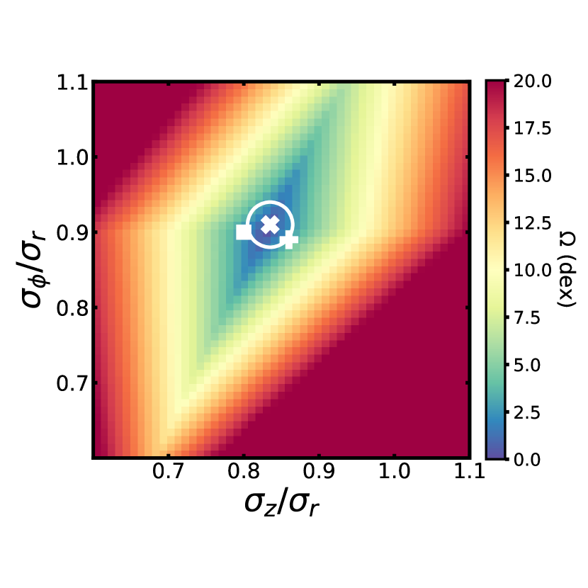
Figure 13.— Quality of fit statistic $\Omega$ describing the slope of the relation between $\sigma_{z}$, $i$, and $\phi$ for a various choices of the velocity dispersion ratios $\sigma_{z}/\sigma_{r}$ and $\sigma_{\phi}/\sigma_{r}$. The global minimum is prominently defined in the region indicated by the white X, with the white circle indicating the $1\sigma$ uncertainty in the measurement. The white $+$ and white square indicate the best-fit values for the MaNGA Primary and Secondary samples respectively.

This result is dependent on whether there is any residual beam smearing in our spaxel sample; if we had not applied a beam smearing correction we would have derived nearly twice the slope for $\sigma_{\rm H\alpha}$ as a function of $i$ or $\phi$. The absence of any trend between $\langle\sigma_{\rm H\alpha}\rangle$ and redshift (see §IV.1) suggests that any such residual effect should be small; however, we confirm this by repeating our exercise using the MaNGA Primary and Secondary galaxy samples which were designed to reach 1.5 and 2.5 effective radii respectively and have median redshifts of $z=0.027$ and $z=0.05$ (see Figure 1 of Law et al., 2021b). While the Secondary sample has velocity dispersions that are about 1.5 km s${}^{-1}\,$ higher than the Primary sample on average (likely due to the greater prevalence of high-SFR objects in the larger cosmological volume), the derived values of $\alpha=0.86/0.80$ and $\beta=0.89/0.90$ for the Primary/Secondary samples respectively. All four values are within about $1\sigma$ uncertainty of our estimate from the whole MaNGA sample, although the subsample $\alpha$ values differ from each other by $2\sigma$. This difference may suggest some residual beam smearing, but may also simply reflect the statistical uncertainty in our measurement.

Our result for the average velocity dispersion ellipsoid of the ionized gas disk in MaNGA galaxies is broadly in keeping with other estimates in the literature. Most immediately, Varidel et al. (2020) estimated $\sigma_{z}/\sigma_{r}=0.80^{0.06}_{-0.05}$ on the basis of 383 galaxies from the SAMI survey. Although these authors fixed $\sigma_{\phi}/\sigma_{r}=1.0$, their result for $\sigma_{z}/\sigma_{r}$ is consistent with ours to within $1\sigma$. Similarly, Leroy et al. (2008, see their Fig. 21) found that $\sigma_{\rm los}$ for HI gas in the THINGS survey increased by about 2 km s${}^{-1}\,$ from $i=0-60^{\circ}$ (albeit within their quoted error bars) with a significant spike at $i>60^{\circ}$ that they ascribe to projection effects, consistent with our Figure 11.

Likewise, Guiglion et al. (2015) estimate $\sigma_{r}$, $\sigma_{\phi}$, and $\sigma_{z}$ for stellar populations in the Milky Way’s Galactic disk using GAIA-ESO spectroscopic observations. Their Figure 12 suggests that $\sigma_{z}/\sigma_{r}=0.61$ and $\sigma_{\phi}/\sigma_{r}=0.71$, and $\sigma_{z}=20$ km s${}^{-1}\,$ for the metal-rich (i.e., young) thin stellar disk. A more recent analysis by Nitschai et al. (2021) using a combination of GAIA EDR3 and SDSS-IV APOGEE spectroscopic observations found similar results, with $\sigma_{z}/\sigma_{r}=0.663$ and $\sigma_{\phi}/\sigma_{r}=0.711$ (see their Table 1).

Although we should not expect the gas disk and the young stellar disk to have identical kinematics, it is nonetheless suggestive that we find similar values for the vertical velocity dispersion, that the radial velocity dispersion is significantly larger than the vertical dispersion, and that the azimuthal dispersion is intermediate between the two. Indeed, since young stars must have formed from HII regions relatively recently and both broadly trace galactic features such as bars and spiral arms, it is perhaps unsurprising that the trends are in general agreement.

We tested this further using morphological classifications drawn from the Galaxy Zoo project (Willett et al., 2013), in which we describe the strength of the bar and/or spiral arms by the level of agreement between individual classifiers on the presence or absence of such a feature (see, e.g., Géron et al., 2021). Our derived values for the ionized gas velocity dispersion ellipsoid in strong vs weak or absent bars/arms show inconclusive deviations from the main galaxy sample, although our value of $\beta=\sigma_{\phi}/\sigma_{r}=1.0$ for the strong-bar subsample is marginally significant at $3\sigma$. The strong-bar subsample also has line-of-sight velocity dispersions that are larger than the unbarred subsample by about 2 km s${}^{-1}\,$ in the most highly-inclined galaxies, suggesting that bars increase the azimuthal velocity dispersion between HII regions on kpc scales. While galaxies with a strong spiral pattern also have velocity dispersions that are 1-2 km s${}^{-1}\,$ larger than those without a clear spiral pattern, this is likely driven by the increased prevalence of strong spiral patterns in higher-mass galaxies (a trend originally established by Elmegreen & Elmegreen, 1987). We investigate both trends in greater detail in a forthcoming contribution.

VI. Discussion

VI.1. Internal dynamics of the HII regions

Far from being unbiased tracers of a uniform ‘ionized gas’ layer, HII regions are distributed according to wherever the local molecular gas density is high enough that it has been able to condense and initiate star formation. This star formation in turn has dramatic effects on the surrounding gas, with the flood of ionizing photons both heating the gas and combining with mechanical feedback from the bright O+B stars to stir additional turbulence in the now-bright HII region (see, e.g., discussion by Osterbrock & Ferland, 2006). The velocity dispersions $\sigma_{\rm H\alpha}$ that we have measured from observations of the bright $\rm H\alpha$ emission line will thus be a combination of thermal pressure within individual HII regions, turbulent motions within those regions, and an overall dispersion between individual HII regions that tells us about the distribution of molecular clouds within the galactic disk.

The thermal pressure in such regions will be determined by their temperatures $T\sim 10^{4}$K, corresponding to a thermal velocity dispersion $\sigma_{\rm Therm}\approx 10$ km s${}^{-1}\,$ (see, e.g., Krumholz & Burkhart, 2016). The non-thermal component of the velocity dispersion $\sigma_{\rm Turb}$ is broadly related to the expansion of the HII region, although the velocity profiles in nearby galaxies may be more accurately described as turbulent (Osterbrock & Ferland, 2006). The strength of this turbulent component may vary significantly between different HII regions and contribute to the observed relation between $\sigma_{\rm H\alpha}$ and total SFR. Indeed, for giant HII regions there is a well-known relation $L_{\rm H\beta}\propto\sigma_{\rm H\beta}^{5}$ between the turbulent velocity dispersion and the total $\rm H\beta$ luminosity of the nebula that is sufficiently well-calibrated (see, e.g., Larson, 1981; Melnick et al., 2021) as to be used for cosmological distance measurements. For typical HII regions however (many of which we expect to contribute to the signal in a given kpc-scale MaNGA beam) values of $\sigma_{\rm Turb}^{2}$ range from 6-16 km s${}^{-1}\,$ across 4 orders of magnitude in $\rm H\alpha$ luminosity (Zaragoza-Cardiel et al., 2015). Since we observed no strong trends in $\sigma_{\rm H\alpha}$ with $\Sigma_{\rm SFR}$ at fixed total SFR (see Figures 9 and 10), we therefore follow Osterbrock & Ferland (2006) and Krumholz & Burkhart (2016) in assuming that $\sigma_{\rm Turb}\approx 10$ km s${}^{-1}\,$ on average. Altogether, we expect that processes internal to the HII regions themselves thus contribute $\sqrt{\sigma_{\rm Therm}^{2}+\sigma_{\rm Turb}^{2}}=14$ km s${}^{-1}\,$ to our $\rm H\alpha$ velocity dispersion measurements.

One way in which we can assess the physical validity of this assumption is to look at the corresponding velocity dispersion of other elements in the MaNGA data as each will have unique properties. In Figure 14 we plot the observed velocity dispersion of the $\rm H\beta$, [S ii] $\lambda 6718+6732$, [N ii] $\lambda 6585$, [O i] $\lambda 6302$, [O ii] $\lambda 3727+3729$, and [O iii] $\lambda 5007$ emission lines relative to that of $\rm H\alpha$.

We note that $\langle\sigma_{\rm H\beta}\rangle$, $\langle\sigma_{\textrm{[S\,{\sc ii}]}}\rangle$, and $\langle\sigma_{\textrm{[N\,{\sc ii}]}}\rangle$, and $\langle\sigma_{\textrm{[O\,{\sc ii}]}}\rangle$ all closely track $\langle\sigma_{\rm H\alpha}\rangle$, albeit offset to larger values by about 5-10%. This offset was previous noted in Law et al. (2021a, see their Figure 16) at $\langle\sigma_{\rm H\alpha}\rangle$ values characteristic of gas ionized by HII regions and may be due to the corresponding selection bias in favor of only the brightest HII regions (since requiring $\rm H\beta$ SNR $>50$ corresponds to a selection cut $\rm H\alpha$ SNR $\geq 150$). $\langle\sigma_{\textrm{[O\,{\sc iii}]}}\rangle$ in contrast shows a markedly different behavior, rising steadily from $\sim 75$% of $\langle\sigma_{\rm H\alpha}\rangle$ at the lowest SFR to roughly equal values at the highest SFR.

This difference is unlikely to be due to any variation in the distribution of HII regions within the galaxy giving rise to $\rm H\alpha$ vs [O iii] emission. Similarly, it should not be an artifact of dust obscuration (since the trend is not observed in $\rm H\beta$), or of differences in the atomic mass-dependent thermal broadening (since the O⁺⁺ and N⁺ ions have comparable mass, and S⁺ is even more massive). Rather, this is likely due to the significantly larger 35.2 eV ionization potential of the O⁺⁺ ion compared to the $\sim 14$ eV ionization potential of the other ions in Figure 14. As a result of the higher ionization potential, [O iii] -emitting gas is located at denser regions deeper within the HII nebula (see, e.g., Byler et al., 2017) for which the turbulent velocity dispersion $\sigma_{\rm Turb}$ is smaller as the ionization front in HII regions generally increases in speed with radius as the density drops (see review by Osterbrock & Ferland, 2006).

Indeed, our finding that $\langle\sigma_{\textrm{[O\,{\sc iii}]}}\rangle<\langle\sigma_{\rm H\alpha}\rangle$ for the MaNGA data is in keeping with well established trends in giant extragalactic HII regions, for which studies from Hippelein (1986) to Bresolin et al. (2020) have noted that $\langle\sigma_{\textrm{[O\,{\sc iii}]}}\rangle$ is systematically $\sim 2$ km s${}^{-1}\,$ less than $\langle\sigma_{\rm H\alpha}\rangle$. The change in $\langle\sigma_{\textrm{[O\,{\sc iii}]}}\rangle/\langle\sigma_{\rm H\alpha}\rangle$ that we observe over the range of total SFR probed by the MaNGA sample of galaxies on the star-forming main sequence may be a product of the variable size of the $O^{++}$ gas as a function of both age and metallicity of the HII region. However, it is perhaps more likely that this trend is an artifact of the increasing velocity dispersion $\sigma_{\rm Mol}$ between individual HII regions in galactic disks. As we show in §VI.2, at low SFR the observed $\rm H\alpha$ velocity dispersion $\sigma_{\rm H\alpha}$ is dominated by the internal HII region dispersions $\sigma_{\rm Therm}$ and $\sigma_{\rm Turb}$, and differences in $\sigma_{\rm Turb}$ due to stratification of different ionization species within HII regions is therefore noticeable in the measured MaNGA velocity dispersions. In contrast, at higher SFR $\sigma_{\rm H\alpha}$ is dominated by $\sigma_{\rm Mol}$, and small differences due to varying $\sigma_{\rm Turb}$ are impossible to discern.

Our observation of [O i] $\lambda 6302$ may be in keeping with this theory as well, as we find that $\langle\sigma_{\textrm{[O\,{\sc i}]}}\rangle/\langle\sigma_{\rm H\alpha}\rangle\approx 1.5$, consistent with [O i] production by neutral gas far out in the nebula. However, [O i] is significantly fainter than $\rm H\alpha$, and our requirement of SNR $>50$ thus limits our sample to just 400 spaxels across 25 galaxies. We are thus unable to conclusively assess any potential trends in $\langle\sigma_{\textrm{[O\,{\sc i}]}}\rangle/\langle\sigma_{\rm H\alpha}\rangle$ with galactic SFR.

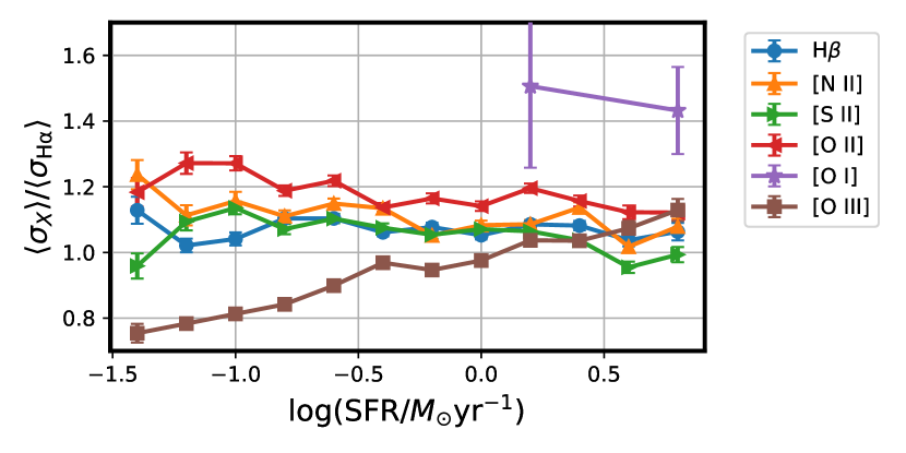
Figure 14.— Ratio between the intensity-weighted mean velocity dispersion of $\rm H\alpha$ and a variety of other strong emission lines as a function of the total $\rm H\alpha$-derived SFR. Colored lines and points show the $2.5$-sigma clipped averages for the MaNGA galaxy sample; error bars represent the uncertainty in the mean.

VI.2. Properties of the Molecular Gas

Assuming that the corrections for thermal velocity dispersion and turbulence within individual HII regions from §VI.1 are (on average) isotropic, we can estimate the vertical velocity dispersion of the disk molecular gas in which individual HII regions are embedded (many of which will typically fall within a $\sim$ kpc-sized MaNGA spatial resolution element) as

$$\sigma_{\rm Mol}^{2}=\sigma_{\rm z}^{2}-\sigma_{\rm Therm}^{2}-\sigma_{\rm Turb}^{2}$$ (10)

where $\sigma_{z}$ is the total vertical velocity dispersion computed following Equation 7 with the best-fit parameters for the velocity ellipsoid derived in §V.

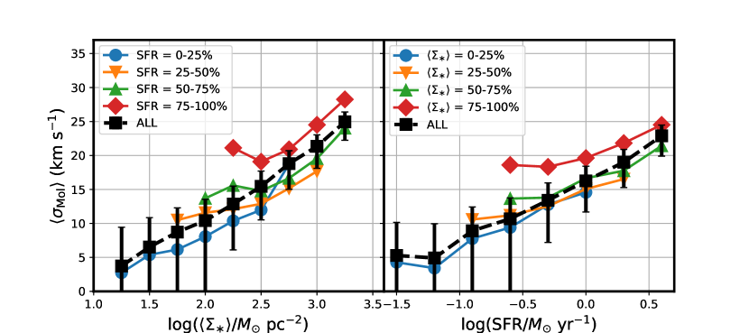
Figure 15.— Velocity dispersion $\sigma_{\rm Mol}$ of the molecular gas (computed as the quadrature difference between the observed ionized gas velocity dispersion and the estimated internal velocity dispersion of the HII regions) as a function of the total SFR and the average disk stellar mass surface density. Colored lines and symbols show the trend for four quartiles in total SFR, while the black lines and symbols show the trend for all MaNGA galaxies. Each point represents the $2.5\sigma$-clipped average of the individual MaNGA data points. Error bars on black point show estimated uncertainty in the mean assuming that the turbulent velocity dispersion is $\sigma_{\rm Turb}=10\pm 5$ km s${}^{-1}\,$. All points represent $2.5\sigma$-clipped means applied to the observational sample.

In Figure 15 we plot $\sigma_{\rm Mol}$ for the MaNGA galaxy sample as a function of the total SFR and the average stellar mass surface density (i.e., one potential candidate for a global disk property that might be expected to scale with the vertical disk velocity dispersion). These values are extremely uncertain; as illustrated by Figure 7 (lower-right panel) the observed velocity dispersion in the lowest SFR bin is approximately 15 km s${}^{-1}\,$, which is statistically indistinguishable from our assumed 14 km s${}^{-1}\,$ (see §VI.1) due to thermal and turbulent motions within individual HII regions. We cannot therefore say with confidence whether $\sigma_{\rm Mol}=2$ km s${}^{-1}\,$ in the lowest SFR (or $\langle\Sigma_{\ast}\rangle$) bin as indicated by Figure 15 or some other small single-digit value. Regardless, under our present assumptions it appears to be the case that in main-sequence galaxies with the lowest SFR the observed ionized gas velocity dispersion is consistent with being entirely produced by physics internal to individual HII regions, while at the highest SFR the observed dispersion is dominated by the velocity dispersion of the molecular gas in which those HII regions are embedded.

Despite the large uncertainties, our estimated $\sigma_{\rm Mol}$ are broadly consistent with estimates of the HI and molecular gas velocity dispersions available in the literature. Ianjamasimanana et al. (2012) for instance reports H I velocity dispersions of 7-17 km s${}^{-1}\,$ for 34 galaxies in the THINGS survey (which they ascribe to two components due to the cold and warm neutral medium respectively). These values are close to the 5-20 km s${}^{-1}\,$ range that we see in Figure 15 for the log(SFR$/M_{\odot}$ yr^-1) $=-1.5$ to 0.5 range of the THINGS survey (Walter et al., 2008). Likewise, Wilson et al. (2019) observed that the CO-based velocity dispersion in local (U)LIRGs increased as the square root of the molecular gas surface density. Although we cannot estimate a meaningful slope to this relation ourselves due to the uncertainty of our correction for thermal and turbulent pressure within the HII regions, we note that we are nonetheless consistent with such a scaling relation- over a factor of 100 in $\Sigma_{\ast}$ Figure 15 suggests that $\sigma_{\rm Mol}$ changes by about a factor of ten.

Molecular gas velocity dispersions have been studied in detail in recent years as well. Hughes et al. (2013) for instance measured the 53-pc matched resolution properties of thousands of molecular clouds in M51, M33 and the LMC and found a range of values from 3-15 km s${}^{-1}\,$. More recently, Sun et al. (2020) studied a sample of 70 nearby galaxies with the PHANGS-ALMA CO survey composed of $>100,000$ independent sightlines. As these authors demonstrated (see their Fig 1), $\sigma_{\rm Mol}$ on 150pc scales is a strong function of the molecular gas surface density, ranging from $\sigma_{\rm Mol}=1$ km s${}^{-1}\,$ to values in excess of 30 km s${}^{-1}\,$ at the highest surface densities. We endeavor to compare our results quantitatively by estimating the average molecular gas surface density of our MaNGA galaxies. We do this by scaling our galaxy-averaged SFR surface densities to $\Sigma_{\rm Mol}$ using the observed mean relation for nearby disk galaxies from the HERACLES CO survey (Leroy et al., 2013, their $\rm H\alpha$$+24\micron$ relation.). In Figure 16 we plot $\sigma_{\rm Mol}$ as a function of $\Sigma_{\rm Mol}$ for the MaNGA data in comparison to the median of the Sun et al. (2020, see their Fig. 1) data; while the overall normalization of both axes is somewhat uncertain, the two data sets more or less agree that $\sigma_{\rm Mol}$ increases rapidly over the range in molecular gas surface densities probed by galaxies on the main sequence. Sun et al. (2020) in particular noted that their results (and by extension ours as well) implied that the molecular gas exceeds its self-gravitational binding energy by a small factor.

On its own, the MaNGA data is unable to conclusively determine whether or not there is a floor to the cold gas velocity dispersion around 10 km s${}^{-1}\,$ as predicted by some galactic disk models (e.g., the Transport+Feedback model of Krumholz et al., 2018). As illustrated by Figure 15, the presence or absence of such a floor is predicated on the nature of the corrections for $\sigma_{\rm Therm}$ and $\sigma_{\rm Turb}$; if $\sigma_{\rm Turb}\geq 10$ km s${}^{-1}\,$ there is no such floor and the observed $\rm H\alpha$ velocity dispersions appear to be explained entirely by HII region physics. If $\sigma_{\rm Turb}=5$ km s${}^{-1}\,$ though, the error bars suggest that the MaNGA data is compatible with a 10 km s${}^{-1}\,$ floor. Given the Sun et al. (2020) ALMA results though, we favor the former explanation in which $\sigma_{\rm Mol}$ continues to decline towards lower SFR.

Theoretical models of the turbulence tend to fall into two broad groups; those in which the turbulence is driven by stellar feedback (e.g., Ostriker & Shetty, 2011; Faucher-Giguère et al., 2013), and those in which the turbulence is driven by gravitational instabilities (e.g., Krumholz & Burkert, 2010). Based on the work of Krumholz & Burkhart (2016), in the first scenario we would expect that the SFR $\propto\sigma_{\rm Mol}^{2}$, while the latter would predict that SFR $\propto f_{g}^{2}\sigma_{\rm Mol}$ where $f_{g}$ is the gas fraction. We evaluate these two possibilities in Figure 17 by plotting $\sigma_{\rm Mol}$ divided by the SFR for the MaNGA galaxies as a function of the gas fraction. In the feedback driven model, $\sigma_{\rm Mol}/SFR\propto SFR^{-1/2}$ with no explicit dependence on the gas fraction. Based on the HI-MaNGA data though we note that in our galaxies SFR $\propto f_{g}^{-2}$ (i.e., total SFR is highest in the highest-mass galaxies for which the average atomic gas fraction is low), implying that $\sigma_{\rm Mol}/SFR\propto f_{g}$. Such a relation is exactly what we see in our data. In contrast, the gravity driven model predicts $\sigma_{\rm Mol}/SFR\propto f_{g}^{-2}$ which is strongly disfavored by the MaNGA observations. At least in the range of conditions present in the $z=0$ galactic main sequence, turbulence therefore appears to be consistent with feedback driven by the observed star formation rate. We note that a similar conclusion was reached by Bacchini et al. (2020), who found that the atomic and molecular gas turbulence in a sample of ten nearby star forming galaxies was energetically consistent with supernova feedback alone after accounting for increased dissipation timescales due to radial flaring of the galactic gas disk.

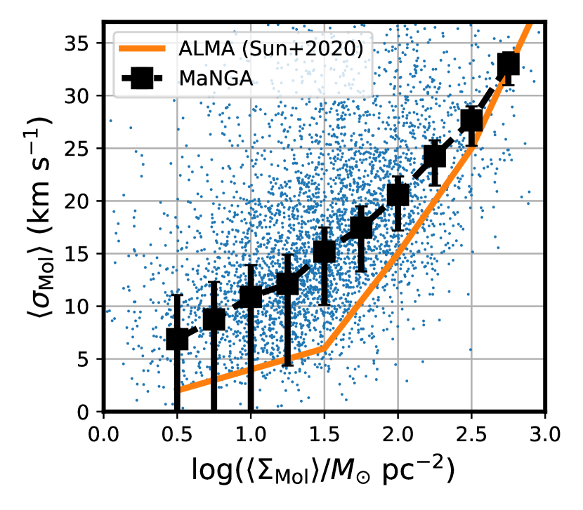
Figure 16.— Estimated molecular gas velocity dispersion as a function of the mean molecular gas surface density for the MaNGA data (small blue points), along with 2.5-$\sigma$ clipped mean values (solid black points). Error bars represent the uncertainty in the mean, which is dominated by the uncertainty in our adopted correction for HII region turbulence $\sigma_{\rm Turb}$. The solid orange line represents the mean observed for 150-pc scale CO PHANGS-ALMA data by Sun et al. (2020).

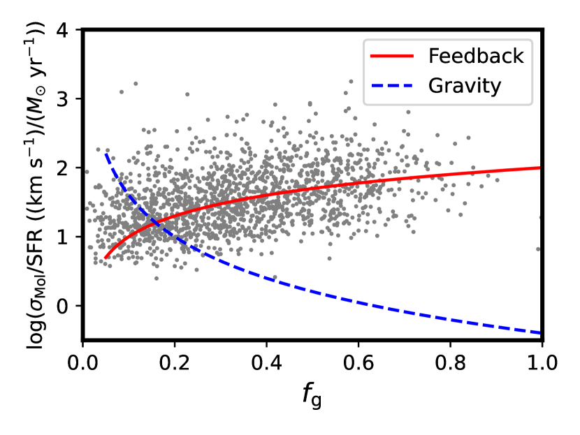
Figure 17.— Estimated mean molecular gas velocity dispersion divided by the total SFR as a function of the atomic gas mass fraction estimated from HI observations for the MaNGA galaxy sample (grey points). Overplotted for comparison are the feedback-based and gravity-based turbulence models (SFR $\propto\sigma_{\rm Mol}^{2}$ and SFR $\propto f_{g}^{2}\sigma_{\rm Mol}$ respectively) described by Krumholz & Burkhart (2016); note that the normalization of the models has been chosen arbitrarily.

Assuming that the molecular gas is in pressure equilibrium with the vertical disk velocity dispersion balancing the gravitational force of the average disk mass surface density it is possible to estimate the effective scaleheight $h$ across which our HII regions are distributed. Following traditional derivations (see, e.g., Wilson et al., 2019; Barrera-Ballesteros et al., 2021), we define

$$h=\sigma_{\rm Mol}^{2}/2\pi G\Sigma_{\rm Tot}$$ (11)

where $\Sigma_{\rm Tot}=\Sigma_{\ast}+\Sigma_{\rm Mol}$.

For the range of values shown in Figures 15 and 16, Equation 11 implies disk scaleheights in the range $\sim 10-40$ pc. While estimates of the molecular gas scaleheight in the Milky Way and other galaxies vary substantially according to the tracer used (e.g., CO emission, [C ii] emission, 870 $\micron$ continuum emission, etc), our values are consistent with those similarly sensitive to the actively star-forming layer; Anderson et al. (2019, and references therein) for instance find a vertical scale height of $\sim 30$pc in the Milky Way based on the observed distribution of Galactic HII regions in the WISE catalog (ranging from 25 pc for the youngest to 40 pc for the oldest such regions). Likewise, at a SFR of $1M_{\odot}$ yr^-1, Figure 15 implies a molecular gas velocity dispersion of $\sigma_{\rm Mol}=15$ km s${}^{-1}\,$, entirely in keeping with the youngest, most metal-rich Galactic stellar populations which have vertical velocity dispersions in the range 10-20 km s${}^{-1}\,$ (Bovy et al., 2012; Hayden et al., 2017).

VI.3. Diffuse Ionized Gas

Thus far, we have concentrated our attention exclusively on the gas ionized by star-forming processes in HII regions, and the corresponding implications for the underlying molecular gas layer. However, star formation is not the only source of H ionizing photons; diffuse ionized gas (DIG) can represent a significant component of the total $\rm H\alpha$ emission from a given galaxy (Oey et al., 2007; Zhang et al., 2017) and offers an additional means by which to study the structure of the ionized gas beyond the confines of traditional HII regions.

As discussed in Law et al. (2021b), DIG can be reliably identified by selecting spaxels with low $\rm H\alpha$ equivalent width that strongly cluster in the traditional LI(N)ER region of the BPT diagram. Using the [S ii]/$\rm H\alpha$ and [O iii]/$\rm H\beta$ criteria established in Law et al. (2021b), we select all DIG-like spaxels in our sample of otherwise star-forming galaxies. By definition, very few such spaxels meet our ideal SNR $>50$ threshold required to minimize biases from the large MaNGA instrumental LSF. We therefore relax this criterion to require SNR $>10$, resulting in a sample of 39,000 spaxels distributed amongst 2935 individual galaxies. While this spaxel sample is just 3% the sample size of star-forming spaxels, it is nonetheless sufficient to draw some general conclusions.

In Figure 18 (open triangles) we plot the intensity-weighted mean $\rm H\alpha$ velocity dispersion of these 2935 MaNGA galaxies as a function of the total galaxy SFR (as estimated from the star-forming spaxels). Unlike for the star-forming spaxels, the sample is strongly biased towards the lowest $\rm H\alpha$ SNR in the sample, and we must therefore correct the intensity-weighted mean values for survival statistics from the large MaNGA instrumental LSF following Figure 15 of Law et al. (2021a). After such a correction (filled red triangles in Figure 18) we note that the velocity dispersion of the DIG in the lowest-SFR systems is nearly indistinguishable from the velocity dispersion of the HII regions, but at the highest SFR is nearly double that of the HII regions.

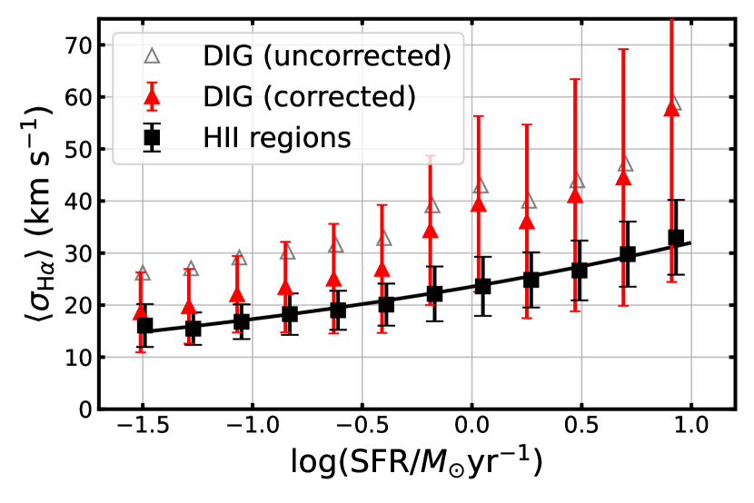
Figure 18.— Intensity-weighted mean velocity dispersion of the diffuse ionized gas within the MaNGA star-forming galaxy sample as a function of the total star-formation rate (derived from the HII regions). Open grey triangles show the binned data for the $\sim 39,000$ spaxels across 2935 individual galaxies meeting our selection criteria. This relation steepens significantly after application of a correction to account for low values lost due to the MaNGA instrumental LSF (solid red triangles). Also shown for comparison are the velocity dispersions for HII regions (filled black squares). Error bars represent the observed width of the galaxy distribution corrected for artificial width due to uncertainties in the instrumental LSF. All points represent $2.5\sigma$-clipped means applied to the observational sample.

We remarked in Law et al. (2021b) that the velocity dispersion of the DIG was larger in general than the velocity dispersion of HII regions; Figure 18 breaks this down into a physical picture of the evolving sources of the DIG with increasing galactic SFR. At low SFR (and low masses) in which there is not a significant evolved stellar population the DIG may be predominantly created by leakage from HII regions, and the overall velocity structure of the HII and DIG gas is thus similar. At higher SFR (and high masses) the galactic stellar disk is much more massive and well-established, and we may be observing the dominant source of the DIG-illuminating photons shifting to hot evolved stars distributed in a much thicker (and higher velocity dispersion) disk.

Such a result is broadly compatible with the observational results of Della Bruna et al. (2020) who noted that the velocity dispersion of the DIG was measurably larger than that of the HII regions at 10pc scales in NGC 7793 observed with the MUSE integral field spectrograph, and of den Brok et al. (2020) who reached similar conclusions based on relative asymmetric drift measurements for 41 galaxies observed with MUSE.

VII. Summary

We have used the completed MaNGA survey to study the behavior of $\rm H\alpha$ velocity dispersions for 4517 star-forming galaxies at $z\sim 0.02$ that sample the star-forming main sequence from $M_{\ast}=10^{9}-10^{11}M_{\odot}$. Despite the large instrumental line spread function, our detailed understanding of systematics allows us to reliably measure ensemble velocity dispersions down to 15-30 km s${}^{-1}\,$ characteristic of the galactic ionized gas disk. We summarize our main conclusions as follows:

• There are strong, well-defined correlations between both the localized SFR surface density $\Sigma_{\rm SFR}$ and the local ionized gas velocity dispersion $\sigma_{\rm H\alpha}$, and between the total galactic SFR and the intensity-weighted mean velocity dispersion $\langle\sigma_{\rm H\alpha}\rangle$. In the latter case, $\langle\sigma_{\rm H\alpha}\rangle$ increases from $16.1\pm 4.1$ km s${}^{-1}\,$ at SFR of 0.03 $M_{\odot}$ yr^-1 to $33.0\pm 7.2$ km s${}^{-1}\,$ at SFR of $8M_{\odot}$ yr^-1. Our results in both cases are consistent with previous measurements from smaller samples of galaxies at higher spectral resolution.

• Using the statistical power of MaNGA to control for a variety of sub-populations, we have demonstrated that trends between ionized gas velocity dispersion $\Sigma_{\rm SFR}$ and stellar mass $M_{\ast}$ are subdominant to the relation with total SFR. That is, total SFR is the strongest driver of the trend in velocity dispersions, and apparent trends with $\Sigma_{\rm SFR}$ and $M_{\ast}$ are produced by the correlation of these quantities with total SFR.

• We have used velocity dispersions derived from multiple nebular emission lines $\rm H\alpha$, $\rm H\beta$, [N ii], [S ii], and [O iii] to constrain our understanding of the ionized gas physics internal to the HII regions that are responsible for the majority of the observed emission. We find that the [O iii] velocity dispersion is systematically smaller than the $\rm H\alpha$ velocity dispersion, consistent with models of HII regions in which the turbulent velocity dispersion $\sigma_{\rm Turb}$ increases with radius within the HII region as the density and ionization parameter decrease.

• Assuming a model for the thermal and turbulent contributions of individual HII regions ($\sigma_{\rm Therm}$ and $\sigma_{\rm Turb}$ respectively), we have estimated the velocity dispersion $\sigma_{\rm Mol}$ of the molecular gas within which the HII regions in our sample are embedded. We find that $\sigma_{\rm Mol}$ increases from $\sim 5$ km s${}^{-1}\,$ at low SFR to $\sim 30$ km s${}^{-1}\,$ at high SFR. Casting our result in terms of the galaxy-averaged cold gas fraction, these results agree closely with recent molecular gas observations from the PHANGS survey.

• The velocity dispersion of the diffuse ionized gas (i.e., $\rm H\alpha$ emission produced by regions with nebular line ratios inconsistent with star-formation models) is comparable to that of the HII-region ionized gas at low SFR and increases more rapidly to $\sim 60$ km s${}^{-1}\,$ in the high-SFR subsample. This may be consistent with a transition from DIG produced mostly by HII-region leakage at low SFR to ionization from hot evolved stars in the more massive stellar disks present at high SFR.

• Using positional information of the spaxels that compose each galaxy, we have assessed the mean velocity dispersion as a function of galaxy inclination $i$ and azimuthal angle $\phi$ within the galaxy. The observed relation suggests that the ionized gas has a velocity dispersion ellipsoid in which the radial and azimuthal velocity dispersions are appreciably larger than the vertical velocity dispersion ($\sigma_{z}/\sigma_{r}=0.84\pm 0.03$ and $\sigma_{\phi}/\sigma_{r}=0.91\pm 0.03$). These ratios differ from unity in the same sense as for the youngest stellar population in the Milky Way, suggesting that young stars and the birth clouds that they come from have similar large-scale influences on their orbital dynamics (e.g., bars and spiral arms within disks).

Overall, the MaNGA data are consistent with a picture in which HII regions condense within localized overdensities in galactic molecular disks. As these HII regions evolve the stars within them, newly freed from the molecular gas disk, gradually diffuse to larger scaleheights as they relax into the gravitational potential of the stellar disk. In the Milky Way, the most metal-rich such stellar populations have scaleheights of order 200 pc, increasing to 400-600 pc for progressively older and more metal-poor populations (Bovy et al., 2012). At higher redshifts $z\sim 2$, the ubiquitously large ionized gas velocity dispersions $\sim 70$ km s${}^{-1}\,$ (e.g. Law et al., 2009; Übler et al., 2019) may imply a similarly large dispersion between HII regions embedded in the molecular gas, fueling the correspondingly thick stellar disk scaleheights that are observed (Law et al., 2012; Zhang et al., 2019). Since main-sequence star-forming galaxies at such redshifts tend to have SFR $\sim 10-100M_{\odot}$ yr${-1}$ (e.g., Wuyts et al., 2011; Theios et al., 2019) typically only seen in (U)LIRGs and similar systems in the nearly universe, the overall picture may be consistent with ‘upside-down’ disk formation in which thick disks form early and thin disks form at later times (e.g., Yu et al., 2021).

References

- Abdurro’uf et al. (2021) Abdurro’uf, Accetta, K., Aerts, C., et al. 2021, arXiv:2112.02026
- Allen et al. (2008) Allen, M. G., Groves, B. A., Dopita, M. A., et al. 2008, ApJS, 178, 20
- Andersen et al. (2006) Andersen, D. R., Bershady, M. A., Sparke, L. S., et al. 2006, ApJS, 166, 505
- Andersen et al. (2013) Andersen, D. R. & Bershady, M. A. 2013, ApJ, 768, 41
- Anderson et al. (2019) Anderson, L. D., Wenger, T. V., Armentrout, W. P., et al. 2019, ApJ, 871, 145. doi:10.3847/1538-4357/aaf571
- Barden et al. (1998) Barden, S. C., Sawyer, D. G., & Honeycutt, R. K. 1998, Proc. SPIE, 3355, 892
- Arribas et al. (2014) Arribas, S., Colina, L., Bellocchi, E., et al. 2014, A&A, 568, A14
- Bacchini et al. (2020) Bacchini, C., Fraternali, F., Iorio, G., et al. 2020, A&A, 641, A70. doi:10.1051/0004-6361/202038223
- Baldwin et al. (1981) Baldwin, J. A., Phillips, M. M., & Terlevich, R. 1981, PASP, 93, 5
- Barrera-Ballesteros et al. (2021) Barrera-Ballesteros, J. K., Sánchez, S. F., Heckman, T., et al. 2021, MNRAS, 503, 3643. doi:10.1093/mnras/stab755
- Belfiore et al. (2016) Belfiore, F., Maiolino, R., Maraston, C., et al. 2016, MNRAS, 461, 3111
- Belfiore et al. (2017) Belfiore, F., Maiolino, R., Tremonti, C., et al. 2017, MNRAS, 469, 151
- Belfiore et al. (2019) Belfiore, F., Westfall, K. B., Schaefer, A., et al. 2019, AJ, 158, 160
- Blanton et al. (2011) Blanton, M. R., Kazin, E., Muna, D., et al. 2011, AJ, 142, 31
- Blanton et al. (2017) Blanton, M. R., Bershady, M. A., Abolfathi, B., et al. 2017, AJ, 154, 28. doi:10.3847/1538-3881/aa7567
- Bovy et al. (2012) Bovy, J., Rix, H.-W., Hogg, D. W., et al. 2012, ApJ, 755, 115. doi:10.1088/0004-637X/755/2/115
- Bovy et al. (2012) Bovy, J., Rix, H.-W., Liu, C., et al. 2012, ApJ, 753, 148. doi:10.1088/0004-637X/753/2/148
- Bresolin et al. (2020) Bresolin, F., Rizzi, L., Ho, I.-T., et al. 2020, MNRAS, 495, 4347. doi:10.1093/mnras/staa1472
- Brinchmann et al. (2004) Brinchmann, J., Charlot, S., White, S. D. M., et al. 2004, MNRAS, 351, 1151
- Brown et al. (2014) Brown, M. J. I., Moustakas, J., Smith, J.-D. T., et al. 2014, ApJS, 212, 18
- Bundy et al. (2015) Bundy, K., Bershady, M. A., Law, D. R., et al. 2015, ApJ, 798, 7
- Byler et al. (2017) Byler, N., Dalcanton, J. J., Conroy, C., et al. 2017, ApJ, 840, 44. doi:10.3847/1538-4357/aa6c66
- Cappellari et al. (2011) Cappellari, M., Emsellem, E., Krajnović, D., et al. 2011, MNRAS, 413, 813
- Cappellari (2020) Cappellari, M. 2020, MNRAS, 494, 4819. doi:10.1093/mnras/staa959
- Cardelli et al. (1989) Cardelli, J. A., Clayton, G. C., & Mathis, J. S. 1989, ApJ, 345, 245. doi:10.1086/167900
- Ceverino et al. (2010) Ceverino, D., Dekel, A., & Bournaud, F. 2010, MNRAS, 404, 2151
- Chabrier (2003) Chabrier, G. 2003, PASP, 115, 763
- Cherinka et al. (2019) Cherinka, B., Andrews, B. H., Sánchez-Gallego, J., et al. 2019, AJ, 158, 74
- Colina et al. (2005) Colina, L., Arribas, S., & Monreal-Ibero, A. 2005, ApJ, 621, 725
- Croom et al. (2012) Croom, S. M., Lawrence, J. S., Bland-Hawthorn, J., et al. 2012, MNRAS, 421, 872
- D’Agostino et al. (2019) D’Agostino, J. J., Kewley, L. J., Groves, B. A., et al. 2019, MNRAS, 487, 4153
- Dekel et al. (2009) Dekel, A., Birnboim, Y., Engel, G., et al. 2009, Nature, 457, 451
- Della Bruna et al. (2020) Della Bruna, L., Adamo, A., Bik, A., et al. 2020, A&A, 635, A134
- den Brok et al. (2020) den Brok, M., Carollo, C. M., Erroz-Ferrer, S., et al. 2020, MNRAS, 491, 4089. doi:10.1093/mnras/stz3184
- Drory et al. (2015) Drory, N., MacDonald, N., Bershady, M. A., et al. 2015, AJ, 149, 77
- Elmegreen & Elmegreen (1987) Elmegreen, D. M. & Elmegreen, B. G. 1987, ApJ, 314, 3. doi:10.1086/165034
- Epinat et al. (2008) Epinat, B., Amram, P., & Marcelin, M. 2008, MNRAS, 390, 466
- Epinat et al. (2010) Epinat, B., Amram, P., Balkowski, C., et al. 2010, MNRAS, 401, 2113
- Faucher-Giguère et al. (2013) Faucher-Giguère, C.-A., Quataert, E., & Hopkins, P. F. 2013, MNRAS, 433, 1970. doi:10.1093/mnras/stt866
- Förster Schreiber et al. (2009) Förster Schreiber, N. M., Genzel, R., Bouché, N., et al. 2009, ApJ, 706, 1364
- Förster Schreiber et al. (2018) Förster Schreiber, N. M., Renzini, A., Mancini, C., et al. 2018, ApJS, 238, 21
- García-Marín et al. (2009) García-Marín, M., Colina, L., & Arribas, S. 2009, A&A, 505, 1017
- Genzel et al. (2011) Genzel, R., Newman, S., Jones, T., et al. 2011, ApJ, 733, 101
- Géron et al. (2021) Géron, T., Smethurst, R. J., Lintott, C., et al. 2021, MNRAS, 507, 4389. doi:10.1093/mnras/stab2064
- Glazebrook (2013) Glazebrook, K. 2013, PASA, 30, 56
- Green et al. (2010) Green, A. W., Glazebrook, K., McGregor, P. J., et al. 2010, Nature, 467, 684
- Green et al. (2014) Green, A. W., Glazebrook, K., McGregor, P. J., et al. 2014, MNRAS, 437, 1070
- Guiglion et al. (2015) Guiglion, G., Recio-Blanco, A., de Laverny, P., et al. 2015, A&A, 583, A91. doi:10.1051/0004-6361/201525883
- Gunn et al. (2006) Gunn, J. E., Siegmund, W. A., Mannery, E. J., et al. 2006, AJ, 131, 2332
- Harrison et al. (2017) Harrison, C. M., Johnson, H. L., Swinbank, A. M., et al. 2017, MNRAS, 467, 1965
- Hayden et al. (2017) Hayden, M. R., Recio-Blanco, A., de Laverny, P., et al. 2017, A&A, 608, L1. doi:10.1051/0004-6361/201731494
- Hayward & Hopkins (2017) Hayward, C. C., & Hopkins, P. F. 2017, MNRAS, 465, 1682
- Hippelein (1986) Hippelein, H. H. 1986, A&A, 160, 374
- Holmberg (1958) Holmberg, E. 1958, Meddelanden fran Lunds Astronomiska Observatorium Serie II, 136, 1
- Hughes et al. (2013) Hughes, A., Meidt, S. E., Colombo, D., et al. 2013, ApJ, 779, 46. doi:10.1088/0004-637X/779/1/46
- Hung et al. (2019) Hung, C.-L., Hayward, C. C., Yuan, T., et al. 2019, MNRAS, 482, 5125
- Ianjamasimanana et al. (2012) Ianjamasimanana, R., de Blok, W. J. G., Walter, F., et al. 2012, AJ, 144, 96
- Johnson et al. (2018) Johnson, H. L., Harrison, C. M., Swinbank, A. M., et al. 2018, MNRAS, 474, 5076
- Jones et al. (2010) Jones, T. A., Swinbank, A. M., Ellis, R. S., et al. 2010, MNRAS, 404, 1247
- Kauffmann et al. (2003) Kauffmann, G., Heckman, T. M., Tremonti, C., et al. 2003, MNRAS, 346, 1055
- Kennicutt (1998) Kennicutt, R. C. 1998, ApJ, 498, 541
- Kewley et al. (2001) Kewley, L. J., Dopita, M. A., Sutherland, R. S., et al. 2001, ApJ, 556, 121
- Krumholz & Burkert (2010) Krumholz, M. & Burkert, A. 2010, ApJ, 724, 895. doi:10.1088/0004-637X/724/2/895
- Krumholz & Burkhart (2016) Krumholz, M. R., & Burkhart, B. 2016, MNRAS, 458, 1671
- Krumholz et al. (2018) Krumholz, M. R., Burkhart, B., Forbes, J. C., et al. 2018, MNRAS, 477, 2716
- Larson (1981) Larson, R. B. 1981, MNRAS, 194, 809. doi:10.1093/mnras/194.4.809
- Law et al. (2009) Law, D. R., Steidel, C. C., Erb, D. K., et al. 2009, ApJ, 697, 2057
- Law et al. (2012) Law, D. R., Shapley, A. E., Steidel, C. C., et al. 2012, Nature, 487, 338
- Law et al. (2012) Law, D. R., Steidel, C. C., Shapley, A. E., et al. 2012, ApJ, 745, 85. doi:10.1088/0004-637X/745/1/85
- Law et al. (2015) Law, D. R., Yan, R., Bershady, M. A., et al. 2015, AJ, 150, 19
- Law et al. (2016) Law, D. R., Cherinka, B., Yan, R., et al. 2016, AJ, 152, 83
- Law et al. (2018) Law, D. R., Steidel, C. C., Chen, Y., et al. 2018, ApJ, 866, 119
- Law et al. (2021a) Law, D. R., Westfall, K. B., Bershady, M. A., et al. 2021, AJ, 161, 52. doi:10.3847/1538-3881/abcaa2
- Law et al. (2021b) Law, D. R., Ji, X., Belfiore, F., et al. 2021, ApJ, 915, 35. doi:10.3847/1538-4357/abfe0a
- Lehnert et al. (2009) Lehnert, M. D., Nesvadba, N. P. H., Le Tiran, L., et al. 2009, ApJ, 699, 1660
- Lehnert et al. (2013) Lehnert, M. D., Le Tiran, L., Nesvadba, N. P. H., et al. 2013, A&A, 555, A72
- Leroy et al. (2008) Leroy, A. K., Walter, F., Brinks, E., et al. 2008, AJ, 136, 2782. doi:10.1088/0004-6256/136/6/2782
- Leroy et al. (2013) Leroy, A. K., Walter, F., Sandstrom, K., et al. 2013, AJ, 146, 19. doi:10.1088/0004-6256/146/2/19
- Martinsson et al. (2013) Martinsson, T. P. K., Verheijen, M. A. W., Westfall, K. B., et al. 2013, A&A, 557, A130
- Masters et al. (2019) Masters, K. L., Stark, D. V., Pace, Z. J., et al. 2019, MNRAS, 488, 3396. doi:10.1093/mnras/stz1889
- Melnick et al. (2021) Melnick, J., Tenorio-Tagle, G., & Telles, E. 2021, A&A, 649, A175. doi:10.1051/0004-6361/201937268
- Moiseev et al. (2015) Moiseev, A. V., Tikhonov, A. V., & Klypin, A. 2015, MNRAS, 449, 3568
- Nguyen et al. (2018) Nguyen, N. K., Pettitt, A. R., Tasker, E. J., et al. 2018, MNRAS, 475, 27. doi:10.1093/mnras/stx3143
- Nitschai et al. (2021) Nitschai, M. S., Eilers, A.-C., Neumayer, N., et al. 2021, ApJ, 916, 112. doi:10.3847/1538-4357/ac04b5
- Oliva-Altamirano et al. (2018) Oliva-Altamirano, P., Fisher, D. B., Glazebrook, K., et al. 2018, MNRAS, 474, 522
- Oey et al. (2007) Oey, M. S., Meurer, G. R., Yelda, S., et al. 2007, ApJ, 661, 801. doi:10.1086/517867
- Oparin & Moiseev (2018) Oparin, D. V., & Moiseev, A. V. 2018, Astrophysical Bulletin, 73, 298
- Orr et al. (2020) Orr, M. E., Hayward, C. C., Medling, A. M., et al. 2020, MNRAS, 496, 1620. doi:10.1093/mnras/staa1619
- Osterbrock & Ferland (2006) Osterbrock, D. E. & Ferland, G. J. 2006, Astrophysics of gaseous nebulae and active galactic nuclei, 2nd. ed. by D.E. Osterbrock and G.J. Ferland. Sausalito, CA: University Science Books, 2006
- Ostriker & Shetty (2011) Ostriker, E. C. & Shetty, R. 2011, ApJ, 731, 41. doi:10.1088/0004-637X/731/1/41
- Pettini & Pagel (2004) Pettini, M., & Pagel, B. E. J. 2004, MNRAS, 348, L59
- Price et al. (2020) Price, S. H., Kriek, M., Barro, G., et al. 2020, ApJ, 894, 91. doi:10.3847/1538-4357/ab7990
- Ryden (2006) Ryden, B. S. 2006, ApJ, 641, 773. doi:10.1086/500497
- Sánchez et al. (2012) Sánchez, S. F., Kennicutt, R. C., Gil de Paz, A., et al. 2012, A&A, 538, A8
- Sánchez et al. (2021a) Sánchez, S. F., Walcher, C. J., Lopez-Cobá, C., et al. 2021, RMxAA, 57, 3. doi:10.22201/ia.01851101p.2021.57.01.01
- Sánchez et al. (2021b) Sánchez, S. F., Barrera-Ballesteros, J. K., Colombo, D., et al. 2021, MNRAS, 503, 1615. doi:10.1093/mnras/stab442
- Shirazi & Brinchmann (2012) Shirazi, M., & Brinchmann, J. 2012, MNRAS, 421, 1043
- Simons et al. (2017) Simons, R. C., Kassin, S. A., Weiner, B. J., et al. 2017, ApJ, 843, 46
- Smee et al. (2013) Smee, S. A., Gunn, J. E., Uomoto, A., et al. 2013, AJ, 146, 32
- Stark et al. (2021) Stark, D. V., Masters, K. L., Avila-Reese, V., et al. 2021, MNRAS, 503, 1345. doi:10.1093/mnras/stab566
- Stott et al. (2016) Stott, J. P., Swinbank, A. M., Johnson, H. L., et al. 2016, MNRAS, 457, 1888
- Sun et al. (2020) Sun, J., Leroy, A. K., Schinnerer, E., et al. 2020, ApJ, 901, L8. doi:10.3847/2041-8213/abb3be
- Swinbank et al. (2012) Swinbank, A. M., Smail, I., Sobral, D., et al. 2012, ApJ, 760, 130. doi:10.1088/0004-637X/760/2/130
- Terlevich & Melnick (1981) Terlevich, R., & Melnick, J. 1981, MNRAS, 195, 839
- Theios et al. (2019) Theios, R. L., Steidel, C. C., Strom, A. L., et al. 2019, ApJ, 871, 128. doi:10.3847/1538-4357/aaf386
- Tremonti et al. (2004) Tremonti, C. A., Heckman, T. M., Kauffmann, G., et al. 2004, ApJ, 613, 898
- Übler et al. (2019) Übler, H., Genzel, R., Wisnioski, E., et al. 2019, ApJ, 880, 48
- Varidel et al. (2016) Varidel, M., Pracy, M., Croom, S., et al. 2016, PASA, 33, 6
- Varidel et al. (2019) Varidel, M. R., Croom, S. M., Lewis, G. F., et al. 2019, MNRAS, 485, 4024
- Varidel et al. (2020) Varidel, M. R., Croom, S. M., Lewis, G. F., et al. 2020, MNRAS, doi:10.1093/mnras/staa1272
- Veilleux & Osterbrock (1987) Veilleux, S., & Osterbrock, D. E. 1987, ApJS, 63, 295
- Wake et al. (2017) Wake, D. A., Bundy, K., Diamond-Stanic, A. M., et al. 2017, AJ, 154, 86
- Walter et al. (2008) Walter, F., Brinks, E., de Blok, W. J. G., et al. 2008, AJ, 136, 2563. doi:10.1088/0004-6256/136/6/2563
- Weiner et al. (2006) Weiner, B. J., Willmer, C. N. A., Faber, S. M., et al. 2006, ApJ, 653, 1027
- Westfall et al. (2019) Westfall, K. B., Cappellari, M., Bershady, M. A., et al. 2019, AJ, 158, 231
- Willett et al. (2013) Willett, K. W., Lintott, C. J., Bamford, S. P., et al. 2013, MNRAS, 435, 2835. doi:10.1093/mnras/stt1458
- Wilson et al. (2019) Wilson, C. D., Elmegreen, B. G., Bemis, A., et al. 2019, ApJ, 882, 5
- Wisnioski et al. (2015) Wisnioski, E., Förster Schreiber, N. M., Wuyts, S., et al. 2015, ApJ, 799, 209. doi:10.1088/0004-637X/799/2/209
- Wuyts et al. (2011) Wuyts, S., Förster Schreiber, N. M., van der Wel, A., et al. 2011, ApJ, 742, 96
- Yan et al. (2016) Yan, R., Tremonti, C., Bershady, M. A., et al. 2016, AJ, 151, 8
- Yan et al. (2016) Yan, R., Bundy, K., Law, D. R., et al. 2016, AJ, 152, 197
- Yan et al. (2019) Yan, R., Chen, Y., Lazarz, D., et al. 2019, ApJ, 883, 175. doi:10.3847/1538-4357/ab3ebc
- Yu et al. (2019) Yu, X., Shi, Y., Chen, Y., et al. 2019, MNRAS, 486, 4463
- Yu et al. (2021) Yu, S., Bullock, J. S., Klein, C., et al. 2021, MNRAS, 505, 889. doi:10.1093/mnras/stab1339
- Yuan et al. (2017) Yuan, T., Richard, J., Gupta, A., et al. 2017, ApJ, 850, 61
- Zaragoza-Cardiel et al. (2015) Zaragoza-Cardiel, J., Beckman, J. E., Font, J., et al. 2015, MNRAS, 451, 1307. doi:10.1093/mnras/stv1024
- Zhang et al. (2017) Zhang, K., Yan, R., Bundy, K., et al. 2017, MNRAS, 466, 3217
- Zhang et al. (2019) Zhang, H., Primack, J. R., Faber, S. M., et al. 2019, MNRAS, 484, 5170. doi:10.1093/mnras/stz339
- Zhou et al. (2017) Zhou, L., Federrath, C., Yuan, T., et al. 2017, MNRAS, 470, 4573