Interpretable Preference-based Reinforcement Learning
with Tree-Structured Reward Functions

Abstract.

The potential of reinforcement learning (RL) to deliver aligned and performant agents is partially bottlenecked by the reward engineering problem. One alternative to heuristic trial-and-error is preference-based RL (PbRL), where a reward function is inferred from sparse human feedback. However, prior PbRL methods lack interpretability of the learned reward structure, which hampers the ability to assess robustness and alignment. We propose an online, active preference learning algorithm that constructs reward functions with the intrinsically interpretable, compositional structure of a tree. Using both synthetic and human-provided feedback, we demonstrate sample-efficient learning of tree-structured reward functions in several environments, then harness the enhanced interpretability to explore and debug for alignment.

1. Introduction

It has recently been argued that the paradigm of reinforcement learning (RL) , in which agents learn action-selection policies by exploration to maximise future reward, is sufficiently general to give rise to most, if not all, aspects of natural and artificial intelligence Silver et al. (2021). However, the origin of the reward signal itself has received limited research attention compared with the algorithms used to optimise it. Singh et al. (2009) argue that the traditional presentation of reward, as a known and hard-wired property of an agent’s environment, is misleading with respect to both biological plausibility and real-world technical applications. Motivated by evolutionary biology, they propose a differentiation between a latent fitness function $F$, which produces a scalar evaluation of the true quality of a behavioural trajectory, and the reward function $R$, which is a mere proxy to convert global pressures on fitness into local pressures on immediate decision-making. $R$ may have a nontrivial relationship to $F$ because it must be tailored to both the learning dynamics of the agent and the structure of the environment. During the learning process, two nested optimisation loops are at work: inner adaptation of the RL agent within a given reward structure $R$, and outer adaptation of $R$ to better align it with fitness.

As RL becomes more powerful, the engineering of aligned reward functions will become “both more important and more difficult” Dewey (2014). The prevailing reliance on heuristic approaches, which already presents challenges to real-world deployment Leike et al. (2018) and hampers the use of RL non-experts Wirth et al. (2017), is likely to prove inadequate in the face of vastly more capable agents which can exploit any specification errors. Several alternatives to heuristic reward engineering have been proposed, including inverse RL Abbeel and Ng (2004), inverse reward design Hadfield-Menell et al. (2017), and advice-taking mechanisms Maclin and Shavlik (1996), all of which involve interaction with a human with (possibly tacit) knowledge of $F$. In this paper, we focus on yet another human-in-the-loop approach, preference-based RL (PbRL) Wirth et al. (2017), in which a reward function is inferred from preferences expressed by the human over sets of candidate behaviours, indicating which have higher fitness. Given a dataset of preference labels, $R$ is constructed to reward commonly-preferred states and actions, and this function is used to train the agent. While ostensibly restrictive, preference feedback places low cognitive demands on the human, requires little domain expertise or training, and tends to yield lower variance than direct fitness labelling since it does not require the human to fix an absolute scale Guo et al. (2018).

The outcome of PbRL is a policy whose true fitness depends on its expected reward under $R$, and the alignment of $R$ to $F$. Without ground-truth knowledge of $F$, it is hard to define quantitative metrics for the latter, which instead becomes a fuzzy, multi-faceted judgement, requiring the assessor to build an intuitive understanding of the structure of $R$ and its effect on agent learning. In large part, this is an interpretability problem. The importance of interpretability for human-in-the-loop RL has been highlighted in surveys Leike et al. (2018); Arzate Cruz and Igarashi (2020), and some post hoc analysis has been applied to learnt reward functions to gain some insight into feature influence Russell and Santos (2019); Michaud et al. (2020), but to our knowledge, there have been no efforts to make $R$ intrinsically interpretable (loosely speaking, human-readable) by constraining its functional form. Indeed, prior works implement reward functions as deep neural networks, or ensembles thereof Christiano et al. (2017), which are notoriously opaque to scrutiny.

We present a PbRL algorithm that learns intrinsically interpretable reward functions from human preferences. Specifically, it yields tree-structured reward functions, formed of independent components associated with disjoint subsets of the state-action space, and defined hierarchically as a binary tree. The tree is incrementally refined as new preference labels arrive, and the traceability of these changes provides a powerful mechanism for monitoring and debugging. Trees afford both diagrammatic and geometric visualisation, textual description as a rule set in disjunctive normal form, and the efficient computation of feature importance metrics. Maintaining an explicit uncertainty estimate for each reward component also facilitates active preference learning based on upper confidence bounds. We evaluate our algorithm on four benchmark RL problems using both synthetic and human feedback, and in both offline and online learning settings. We observe aligned and sample-efficient learning of tree-structured reward functions in each of these contexts, alongside some informative failure cases. We then harness the enhanced interpretability to explore and debug for alignment.

This paper is structured as follows. Section 2 reviews the general PbRL problem definition, section 3 introduces the additional tree-structuring constraint that we apply to improve interpretability, and section 4 presents our algorithm for approximately solving the constrained problem. Section 5 gives experimental results with a focus on quantitative performance metrics, while section 6 uses case studies to demonstrate the qualitative interpretability benefits of the tree structure for the purpose of alignment. Finally, section 7 briefly concludes and discusses directions for future work.

2. PbRL Problem Definition

The PbRL problem is formalised within a Markov Decision Process without reward (MDP\R) Abbeel and Ng (2004), in which at discrete time $t$, an agent’s action $a_{t}\in\mathcal{A}$ influences the evolution of an environmental state $s_{t}\in\mathcal{S}$ according to a Markovian dynamics function $D(s_{t+1}|s_{t},a_{t})$. We specifically consider fixed-length episodic MDP\Rs, in which $t$ is initially $0$, $s_{0}$ is sampled from an initial distribution $P_{0}$, and the process deterministically terminates at a fixed $t=T$. The events of an episode are described by a trajectory in state-action space, $\tau=((s_{0},a_{0}),...,(s_{{T-1}},a_{{T-1}}))\in(\mathcal{S}\times\mathcal{A})^{T}$. There also exists a human observer, who evaluates the quality of trajectories according to the latent fitness function $F:(\mathcal{S}\times\mathcal{A})^{T}\rightarrow\mathbb{R}$. The ultimate goal of the agent is to learn an action selection policy $\pi(a_{t}|s_{t})$ that maximises the expected fitness over induced trajectories:

$$\underset{\pi}{\text{argmax}}\ \mathbb{E}_{\tau_{i}\sim\text{Pr}(\tau|P_{0},D,\pi)}F(\tau_{i}).$$ (1)

In order to learn about $F$, the agent must interact with the human. In PbRL, we assume the human cannot specify the analytical form of $F$, or even evaluate it absolutely for a given trajectory, but can only assess the relative fitness of a trajectory pair $\tau_{i},\tau_{j}$ and provide a label $y_{ij}\in[\varepsilon,1-\varepsilon]$ indicating their assessment of the probability that $\tau_{i}$ has higher fitness than $\tau_{j}$ (denoted by $\tau_{i}\succ\tau_{j}$). Here, $\varepsilon\in(0,0.5]$ is a noise parameter preventing extreme probabilities. Agent-human interaction therefore consists of sampling trajectory pairs from a distribution $\psi:((\mathcal{S}\times\mathcal{A})^{T})^{2}\rightarrow[0,1]$ and obtaining preference labels in response. The inference of $F$ reduces to minimising some loss $\ell$ over labelled pairs:

$$\underset{F}{\text{argmin}}\ \mathbb{E}_{(\tau_{i},\tau_{j})\sim\psi}\ \ell(y_{ij},P(\tau_{i}\succ\tau_{j}|F)).$$ (2)

Here, $P$ is a statistical model of human preference labels given estimated fitness values for a trajectory pair, whose definition is an assumption of the modelling process. Applying a basic rationality hypothesis, we can assume that the probability of the human preferring $\tau_{i}$ to $\tau_{j}$ is a monotonically non-decreasing function of the fitness difference $F(\tau_{i})-F(\tau_{j})$. Specifically, we adopt Thurstone’s law of comparative judgement Thurstone (1927), which models the fitness of a set of $n$ trajectories $F(\tau_{1}),...,F(\tau_{n})$ as a multivariate normal distribution with mean $\boldsymbol{\mu}\in\mathbb{R}^{n}$ and covariance $C\in\mathbb{R}^{n\times n}$. This leads to the following preference model:

$$P(\tau_{i}\succ\tau_{j}|\boldsymbol{\mu},C)=\Phi\left(\frac{\boldsymbol{\mu}_{i}-\boldsymbol{\mu}_{j}}{\sqrt{C_{ii}+C_{jj}-2C_{ij}}}\right),$$ (3)

where $\Phi$ is the standard normal cumulative distribution (CDF).

Following the classic approach of Mosteller (1951), we note that under Thurstone’s model, a label $y_{ij}$ implies that the variance-scaled difference in fitness between $\tau_{i}$ and $\tau_{j}$ is proportional to $\Phi^{-1}(y_{ij})$, where $\Phi^{-1}$ is the inverse normal CDF. Therefore, a suitable choice for the labelling loss $\ell$ is the squared error in this variance-scaled fitness difference. Equation 2 can be rewritten as

$$\underset{\boldsymbol{\mu},C}{\text{argmin}}\ \mathbb{E}_{(\tau_{i},\tau_{j})\sim\psi}\left[\Phi^{-1}(y_{ij})-\frac{\boldsymbol{\mu}_{i}-\boldsymbol{\mu}_{j}}{\sqrt{C_{ii}+C_{jj}-2C_{ij}}}\right]^{2}.$$ (4)

For the agent to perform the optimisation in equation 1, $\boldsymbol{\mu}$ and $C$ must be parameterised in a way that generalises to unlabelled trajectories. We adopt a linear model $\boldsymbol{\mu}_{i}=\textbf{r}^{\top}\textbf{n}_{i},\ C_{ij}=\textbf{n}_{i}^{\top}\Sigma\textbf{n}_{j},\ \forall i,j\in\{1..n\}$, where $\textbf{n}_{i}\in\mathbb{R}^{m}$ is a feature vector summarising the trajectory, $\textbf{r}\in\mathbb{R}^{m}$ is a vector of weights, and $\Sigma\in\mathbb{R}^{m\times m}$ is a covariance matrix associated with r. As in several prior works Abbeel and Ng (2004); Akrour et al. (2012); Christiano et al. (2017), we add a second level of decomposition by defining $\phi:\mathcal{S}\times\mathcal{A}\rightarrow\mathbb{R}^{m}$ as a function that constructs feature vectors from individual state-action pairs, and $\textbf{n}_{i}=\sum_{t=0}^{T-1}\phi(s_{it},a_{it})$ as the unweighted feature expectation over $\tau_{i}$. By the linearity of the normal distribution, it follows that $\boldsymbol{\mu}_{i}-\boldsymbol{\mu}_{j}=\textbf{r}^{\top}(\textbf{n}_{i}-\textbf{n}_{j})$ and $C_{ii}+C_{jj}-2C_{ij}=(\textbf{n}_{i}-\textbf{n}_{j})^{\top}\Sigma(\textbf{n}_{i}-\textbf{n}_{j})$. The final form of equation 2 is thus

$$\underset{\phi,\textbf{r},\Sigma}{\text{argmin}}\ \mathbb{E}_{(\tau_{i},\tau_{j})\sim\psi}\left[\Phi^{-1}(y_{ij})-\frac{\textbf{r}^{\top}(\textbf{n}_{i}-\textbf{n}_{j})}{\sqrt{(\textbf{n}_{i}-\textbf{n}_{j})^{\top}\Sigma(\textbf{n}_{i}-\textbf{n}_{j})}}\right]^{2}.$$ (5)

The decomposition also allows us to rewrite equation 1 as

$$\underset{\pi}{\text{argmax}}\ \mathbb{E}_{\tau_{i}\sim\text{Pr}(\tau|P_{0},D,\pi)}\sum_{t=0}^{T-1}\textbf{r}^{\top}\phi(s_{it},a_{it}),$$ (6)

which is structurally identical to the conventional RL objective of maximising (undiscounted) return in an MDP with reward. Thus, once the agent has inferred the function $\phi$ and vector r it can define a reward function $R(s,a)=\textbf{r}^{\top}\phi(s,a)$, then employ any unmodified RL algorithm to learn a policy $\pi$. As alluded to in the Introduction, $R$ thereby serves as a proxy for $F$, with the true fitness of $\pi$ being a function of both its expected return under $R$ (equation 6) and the alignment of $R$ to $F$, which is approximated by the labelling loss (equation 5). Given that equation 6 is the domain of standard RL, the contribution of this paper is an algorithm for approximately solving equation 5, subject to the particular interpretability constraint outlined in the following section.

3. Interpretability Constraint

We now introduce the key assumption that differentiates our approach from prior work and enables interpretability. That is, we constrain the feature function $\phi$ so that for all $(s,a)\in\mathcal{S}\times\mathcal{A}$, $\phi(s,a)$ is a one-hot vector. This effectively induces a partition of the state-action space into $m$ disjoint subsets, which map to the $m$ possible one-hot vectors. For trajectory $\tau_{i}$, $\textbf{n}_{i}$ can be interpreted as the number of timesteps spent in each subset, and the reward vector r as a set of components that reward state-action pairs according to the subsets they fall within. We model reward components as independent, so that $\Sigma$ is a diagonal matrix. Furthermore, the partition induced by $\phi$ has a binary tree structure, with the $m$ subsets as leaves, connected by a hierarchy of internal nodes emanating from a root. Each internal node applies a test to the state-action pair $(s,a)$. If the test is passed, the logical flow proceeds to the “right” child node. Otherwise, it proceeds to the “left” child. Testing continues until a leaf node $x\in\{1..m\}$ is reached, the state-action pair is mapped to the corresponding one-hot vector, and the reward is given as the corresponding component $\textbf{r}_{x}$ with variance $\Sigma_{xx}$. Although most of our algorithm does not rely on this assumption, we focus here on Euclidean state and action spaces $\mathcal{S}=\mathbb{R}^{D_{s}}$, $\mathcal{A}=\mathbb{R}^{D_{a}}$, in which a state-action pair is a vector $(s,a)\in\mathbb{R}^{D}$, where $D=D_{s}+D_{a}$. Internal node tests have the form $(s,a)_{d}\geq c:d\in\{1..D\}$, which evaluates whether the $d$th element of $(s,a)$ meets or exceeds a threshold $c$. Consequently, each state-action subset has the geometry of an axis-aligned hyperrectangle. Figure 1 provides an illustrative example.

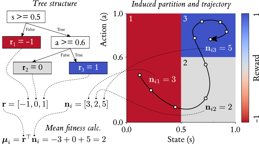
Figure 1. Tree and induced partition for a simple case with $D_{s}=D_{a}=1$ and $m=3$. For a trajectory $\tau_{i}$, $\textbf{n}_{i}$ counts the timesteps (white circles) spent in each subset, and its dot product with r gives the mean fitness estimate $\boldsymbol{\mu}_{i}$. Each component also has a variance $\Sigma_{xx}$, which can be used to compute the trajectory fitness variance $C_{ii}=n_{i}\Sigma n_{i}$ (not shown).

4. Proposed Algorithm

We now present an algorithm for optimising equation 5 subject to the tree-structuring constraint on $\phi$, alongside an active learning scheme that adapts the sampling distribution $\psi$ to focus on trajectories with high-variance fitness estimates and correct overestimation errors. As the algorithm iterates over stages of preference elicitation, reward component fitting, tree structure refinement and distribution updates, there is no single first step. We have tried to order the following subsections to maximise comprehensibility.

Remark

The indirect, multi-stage optimisation approach described here was converged on after extensive experimentation with alternatives, which we outline in Appendix B. The final approach is computationally efficient, easy to implement, and yields reward functions that are significantly more robust to small data changes than the alternatives.

4.1. Preference Elicitation and Representation

We first outline the process of sampling trajectory pairs and storing preference labels. We assume a finite data setting, in which the trajectory space $(\mathcal{S}\times\mathcal{A})^{T}$ is approximated by a sequence of $n$ trajectories $\mathcal{T}=(\tau_{1},...,\tau_{n})$, and the domain of $\psi$ is restricted to $\mathcal{T}^{2}$. This distribution can thus be written as a matrix $\Psi\in[0,1]^{n\times n}:\sum_{ij}\Psi_{ij}=1,\Psi_{ii}=0,\ \forall i\in\{1..n\}$. For the moment, let us take both $\mathcal{T}$ and $\Psi$ as given; we discuss their origins in section 4.5. An instance of preference feedback is obtained by sampling a trajectory pair $\tau_{i}$, $\tau_{j}$ with probability $\Psi_{ij}$, presenting the pair (e.g. by visualisation) to a human, and recording the resultant preference label $y_{ij}\in[\varepsilon,1-\varepsilon]$. We represent a set of $k$ feedback instances by three data structures, a set $\mathcal{P}$, a matrix $A\in\{-1,0,1\}^{k\times n}$ and a vector $\textbf{y}\in\mathbb{R}^{k}$, which are incrementally assembled as preferences arrive. After sampling the $k$th pair $\tau_{i},\tau_{j}$ and observing $y_{ij}$, we add $\{\tau_{i},\tau_{j}\}$ to $\mathcal{P}$, append a row to $A$ in which the $i$th element is $1$, the $j$th element is $-1$ and all other elements are $0$, and append $\textbf{y}_{k}=y_{ij}$. $\mathcal{P}$ thus serves as a record of which pairs have been sampled. $A$ and y allow us to express equation 5 in matrix form as follows:

$$\underset{\phi,\textbf{r},\Sigma}{\text{argmin}}\ \left[\Phi^{-1}(\textbf{y})-(\text{diag}(NA^{\top}\Sigma AN^{\top})^{-\frac{1}{2}})^{\top}AN^{\top}\textbf{r}\right]^{2}.$$ (7)

Here, $N$ is the $m\times n$ matrix of columnar feature vectors $\textbf{n}_{i}$. This notation is used in equations throughout this section.

4.2. Trajectory-Level Fitness Estimation

Direct optimisation of equation 7 subject to the tree-structuring constraint is computationally intractable, so we approximate the global problem by a sequence of local ones. First, we temporarily apply Thurstone’s Case V reduction Thurstone (1927), which assumes unit standard deviations for all fitness differences, i.e. $\text{diag}(NA^{\top}\Sigma AN^{\top})^{\frac{1}{2}}=\mathbbm{1}_{m}$, so simplifies the bracketed expression in equation 7 to $\Phi^{-1}(\textbf{y})-AN^{\top}\textbf{r}$. Following the method developed by Morrissey and Gulliksen (1956), we then use least squares to compute a somewhat biased (by the Case V assumption) estimate of $N^{\top}\textbf{r}=\boldsymbol{\mu}$, which is the $n\times 1$ vector of mean fitness estimates at the level of complete trajectories:

$$N^{\top}\textbf{r}=\boldsymbol{\mu}\approx\tilde{\boldsymbol{\mu}}=(A^{\top}A)^{-1}A^{\top}\Phi^{-1}(\textbf{y}).$$ (8)

4.3. Independent Reward Component Fitting

We then use the trajectory-level estimates $\tilde{\boldsymbol{\mu}}$ to fit the means and variances of the reward components. This is a kind of temporal credit assignment problem: how does each component contribute to the overall fitness of a trajectory $\tau_{i}$? To solve it, we recall that under our tree-structuring constraint, $N_{xi}$ is the number of timesteps $\tau_{i}$ spends in the $x$th state-action subset. A priori, we cannot know which timesteps are responsible for the fitness of $\tau_{i}$, so the least strong assumption is a uniform temporal prior, that the reward component for this subset contributes a fraction $N_{xi}/T$ of the fitness. We can thereby compute an empirical estimate of the $x$th reward component mean by taking a weighted sum over trajectories:

$$\textbf{r}_{x}=\frac{\sum_{\tau_{i}\in\mathcal{P}}\frac{N_{xi}}{T}\tilde{\boldsymbol{\mu}}_{i}}{\sum_{\tau_{i}\in\mathcal{P}}N_{xi}}.$$ (9)

Note that this summation is only over trajectories for which at least one preference label has been provided (denoted, in a slight abuse of notation, by $\tau_{i}\in\mathcal{P}$). We then use $\tilde{\boldsymbol{\mu}}$ and $\textbf{r}_{x}$ to empirically estimate the variance of the $x$th component, $\Sigma_{xx}$:

$$\Sigma_{xx}=\frac{\text{RSS}(N_{x})}{\sum_{\tau_{i}\in\mathcal{P}}N_{xi}};\ \ \ \ \ \text{RSS}(N_{x})=\sum_{\tau_{i}\in\mathcal{P}}N_{xi}\left[\frac{\tilde{\boldsymbol{\mu}}_{i}}{T}-\textbf{r}_{x}\right]^{2}.$$ (10)

The residual sum of squares $\text{RSS}(\cdot)$ is a useful intermediate function that we use again below. By this method, reward components are fitted independently, using only the corresponding rows of $N$. The independent treatment of components leaves $\Sigma$ as a diagonal matrix.

4.4. Tree Structure Refinement

So far, we have assumed a fixed $N$ matrix, and thus a fixed feature function $\phi$, but this function can be modified by adding or removing internal nodes in the tree structure described above. Consider splitting the $x$th leaf node into two by replacing it with an internal node which tests whether the $d$th element of the $(s,a)$ vector exceeds a threshold $c$. The effect of this split on the feature matrix $N$ is to replace the $x$th row of $N$ with a new $2\times n$ matrix, denoted by $N^{[xdc]}$, representing how the number of timesteps each trajectory spends in the $x$th state-action subset is distributed between two new child subsets contained within it. Using the two rows of $N^{[xdc]}$, reward components for the child subsets can be fitted using equations 9 and 10. All other reward components remain unchanged. Repeatedly making such splits grows the tree, each time increasing the number of leaves, subsets and associated reward components $m$ by $1$.

Whenever the trajectory-level fitness estimates $\tilde{\boldsymbol{\mu}}$ are updated, our algorithm grows the existing tree by recursive splitting up to a maximum $m=m_{\text{max}}$, at each step choosing a component to split $x$, splitting dimension $d$ and threshold $c$ to greedily minimise the total residual sum of squares $\sum_{x=1}^{m}\text{RSS}(N_{x})$, and thus achieve a better fit to $\tilde{\boldsymbol{\mu}}$. Since reward components are fitted independently, a single step of this optimisation process can be expressed as follows:

$$\underset{1\leq x\leq m}{\text{max}}\ \underset{1\leq d\leq D}{\text{max}}\ \underset{c\in\mathcal{C}_{d}}{\text{max}}\ \text{RSS}(N_{x})-\text{RSS}(N^{[xdc]}_{1})-\text{RSS}(N^{[xdc]}_{2}).$$ (11)

$\mathcal{C}_{d}$ is a set of candidate split thresholds along dimension $d$. In our experiments, where dataset sizes are moderate, we exhaustively search over all values that occur in labelled trajectories: $\mathcal{C}_{d}=\{(s,a)_{d},\ \forall(s,a)\in\tau,\ \forall\tau\in\mathcal{P}\}$. Crucially, the RSS-based splitting criterion in equation 11 is precisely the one used in classical regression tree learning Breiman et al. (2017). Our algorithm thus utilises a virtually-unmodified, highly-optimised, regression tree implementation.

Once $m_{\text{max}}$ is reached, we then iterate backwards through the growth process, pruning the tree back until $m=1$. At each step in this backward pass, we use the corresponding $N$, r and $\Sigma$ to evaluate the labelling loss expression given in equation 7 (i.e. the global objective that we aim to optimise). To this labelling loss, we add a complexity regularisation term $\alpha m$ to modulate the tradeoff between predictive accuracy and interpretability (through compactness) and also to mitigate overfitting. We identify the tree size that minimises the regularised labelling loss, and use this tree as the updated $\phi$.

4.5. Trajectory Pair Sampling Distribution

Our algorithm works in two data settings: offline and online. In the offline setting, the underlying trajectory dataset $\mathcal{T}$ remains fixed but the sampling matrix $\Psi$ is modified over time. In the online setting, both $\Psi$ and $\mathcal{T}$ change, with the latter being gradually augmented with new trajectories. This makes it possible to use trajectory data generated by the PbRL agent itself as it learns a policy in real-time.

Offline setting

A wide variety of active preference learning schemes have been proposed for PbRL Talati et al. (2021). Partly inspired by existing work in the bandit literature Carpentier et al. (2011); Zoghi et al. (2014) we adopt an upper confidence bound (UCB) strategy, which weights trajectory pairs according to optimistic estimates of their summed fitness. This strategy prioritises trajectories with highly uncertain fitness under the current model, for which additional preference labels are likely to be most useful for reducing uncertainty (in this respect, it is similar to Christiano et al. (2017)). Additionally, the optimism induces a bias towards identifying and correcting cases where trajectory fitness is overestimated, ultimately yielding a conservative reward function which counteracts the well-known overestimation bias in value-based RL Fujimoto et al. (2018). Finally, biasing the preference dataset towards promising trajectories leads the reward function to prioritise distinguishing between high and very high fitness behaviour (rather than low vs very low), which reduces the risk of an agent stagnating at mediocre fitness with no incentive to improve. To implement the UCB strategy we use $N$, r and $\Sigma$ to compute a vector of optimistic fitness values:

$$\textbf{u}=\boldsymbol{\mu}+\lambda\ \text{diag}(C)^{\frac{1}{2}}=N^{\top}\textbf{r}+\lambda\ \text{diag}(N^{\top}\Sigma N)^{\frac{1}{2}},$$ (12)

where $\lambda\geq 0$ determines the number of standard deviations added to the mean. We then construct an $n\times n$ weighting matrix as follows:

$$W^{\text{off}}_{ij}=\left\{\begin{array}[]{ll}0&\text{if }i=j\text{ or }\{\tau_{i},\tau_{j}\}\in\mathcal{P},\\ &\text{or }(\mathcal{P}\neq\emptyset\text{ and }\tau_{i}\not\in\mathcal{P}),\\ \textbf{u}_{i}+\textbf{u}_{j}+\delta&\text{otherwise,}\end{array}\right.\ \ \begin{array}[]{ll}\forall i\in\{1..n\},\\ \forall j\in\{1..n\}.\end{array}$$ (13)

Here, the three “zeroing” conditions respectively prevent comparing a trajectory to itself, prevent repeated pairs, and ensure that one of any sampled pair has already received feedback. The offset $\delta$ is calibrated so that the minimum element not matching a zeroing condition is set to $0$. If all elements match a zeroing condition, then all possible trajectory pairs have been sampled and the process must be halted. Otherwise, we define $\Psi=W^{\text{off}}/\sum_{ij}W^{\text{off}}_{ij}$.

Online setting

If $\mathcal{T}$ monotonically expands with new trajectories over time, but preference labels are obtained at a constant rate, it is possible to show that a higher density of labels is given to trajectory pairs that appear earlier, creating a strong earliness bias in the preference dataset. Assuming a total labelling budget $k_{\text{max}}$ and known final trajectory count $n_{\text{max}}$, we correct for this bias by collecting a batch of labels every time $f_{l}$ new trajectories are added, using monotonically-increasing batch sizes. On the $b$th batch, we define $W^{\text{on}}$ the same as $W^{\text{off}}$, with the extra condition that $W^{\text{on}}_{ij}=0$ if $i\leq f_{l}(b-1)$ and $j\leq f_{l}(b-1)$, which ensures that at least one of $i$ and $j$ are in the most recent $f_{l}$ trajectories. We compute $\Psi$ by normalising $W^{\text{on}}$ as above, then sample $k_{b}$ trajectory pairs, where

$$k_{b}=\text{round}\left(k_{\text{max}}\frac{f_{l}^{2}(2b-1)-f_{l}}{n_{\text{max}}(n_{\text{max}}-1)}\right).$$ (14)

We refer the reader to Appendix C for a more detailed justification of this approach and a derivation of equation 14. Note that the offline setting is recovered by setting $f_{l}=n_{\text{max}}=|\mathcal{T}|$.

4.6. Complete Algorithm

Our algorithm initiates with one reward component ($m=1$) and $\textbf{r}=[0]$, $\Sigma=[0]$. During batch $b$, labelling is paused every $f_{u}$ samples for an iteration of trajectory-level fitness estimation, reward component fitting and tree refinement. This leads to a modified u vector, which alters the sampling matrix for the rest of the batch. In the online setting, where an RL agent uses the learnt reward to train a policy in real-time, the latest $\phi$ and r are used as soon as an update is made. Otherwise, the algorithm runs until the budget $k_{\text{max}}$ is expended, and the final fixed reward is used to train a policy at a later time. A pseudocode algorithm is given in Appendix D.

5. Performance Results

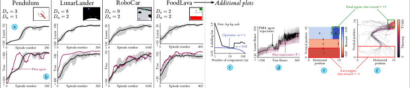
Figure 2. Performance in offline setting using oracle feedback; additional plots shown for FoodLava.

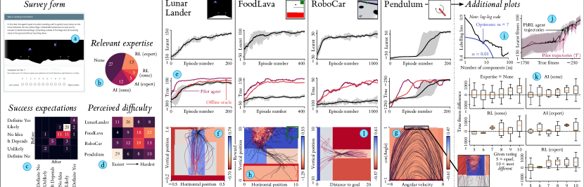
Figure 3. Performance in offline setting using human feedback; additional plots shown for Pendulum.

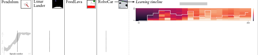
Figure 4. Performance in online setting using oracle feedback; learning timeline shown for RoboCar.

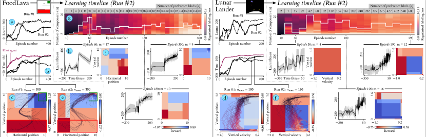
Figure 5. Performance in online setting using human feedback; results with learning timelines for FoodLava and LunarLander.

We have evaluated our algorithm in four RL environments under various learning conditions. In all cases we used a feedback budget $k_{\text{max}}$ between $600$ and $620$, equating to $\approx 1$ hour of human time. Full experimental details are reported in Appendix E; below we discuss our findings by reference to the blue annotation letters in figures 2-5. Key findings are in bold and summarised at the end.

5.1. Offline with Oracle Feedback (Figure 2)

Here, $\mathcal{T}$ was fixed, and comprised of trajectories generated by an RL agent (the pilot agent) as it trained on each environment’s default, hand-engineered reward function. Preference labels came from a synthetic oracle with query access to this reward function. We then trained a second agent (the PbRL agent) on the learnt reward, and finally measured the PbRL agent’s alignment to the original reward function, which was taken to represent ground-truth fitness; see Ibarz et al. (2018) for a similar method of quantitative evaluation. We show learning curves (time series of fitness per episode) for both learnt (a) and ground-truth (b) reward ($5$ repeats; mean and min-max range shown). The consistent monotonicity of the former indicates that tree-structured reward functions gave rise to stable agent learning in all cases, and the latter confirm that this learning was well-aligned with the ground-truth. For Pendulum and RoboCar, asymptotic fitness was indistinguishable from the pilot, while for LunarLander and FoodLava, it was slightly below. We show additional plots for FoodLava. (c) shows that the $\alpha m$-regularised labelling loss was minimised by a tree with $9$ leaves, hence $9$ reward components. (d) gives another measure of alignment by plotting true vs learnt fitness ($\pm 1$ std) for both the pilot trajectories $\mathcal{T}$ and those generated during PbRL agent training. In both cases there is a clear positive correlation, although the relationship for the latter is noisier, suggesting a degree of distributional shift. (e) visualises the $9$ reward components over the two state dimensions as coloured rectangles. The components are arranged isomorphically to the maze layout, with negative reward in the red “lava” region and positive reward around the green “food”. However, some misalignment is visible as high-reward component $8$ is too large in the vertical direction. Referring to (f), which plots the final $10$ trajectories of all $5$ PbRL repeats, we see that this misalignment led to policies that sometimes terminated just below the food.

5.2. Offline with Human Feedback (Figure 3)

Using the same pilot trajectories as $\mathcal{T}$, we then gathered preference data from $62$ human participants via a survey (a) then trained PbRL agents using the resultant reward functions. We asked participants to indicate their level of relevant expertise (b) and expectations of the likelihood of our method succeeding, both before and after completing the survey (c), and to rank the tasks by perceived difficulty of giving feedback (d). Notably, this ranking turned out to predict the success of our method in this setting, since for LunarLander and Pendulum we achieved asymptotic ground-truth fitness (e) only slightly below the oracle results. Information about the ground-truth was not used anywhere in this experiment, which instead relied on participants’ intuitive understanding of the tasks. The fact that it could nonetheless be well-optimised by the resultant PbRL agents indicates that for LunarLander and Pendulum, human intuition was broadly aligned with the default reward functions. Again, the coloured rectangle plots (f) and (g) provide insight into the learnt reward structure, with high reward in LunarLander given in a column above the landing zone, and in Pendulum given when the pole is upright with small angular velocity. The final $10$ trajectories from the PbRL runs are overlaid, showing that the agents sought out high-reward regions and consequently solved the respective landing and pole-balancing tasks. We were unable to achieve aligned learning in FoodLava and RoboCar, although in the former the outcome was not as catastrophic as the learning curve suggests. As can be seen in the rectangle/trajectory plot (h), the PbRL agent learnt to solve most of the maze but was not incentivised to proceed to the food, since a large positive reward component covered the entire upper third. This, we hypothesise, is evidence of a causal confusion problem: within the pilot run dataset, most trajectories that reached the upper third then went on to the food, so our uniform temporal credit assignment was unable to determine that the latter step was necessary for a favourable preference label. A similar issue arose in RoboCar, which we focus on in our interpretability analysis (section 6). For Pendulum, we include the labelling loss curve (i) and alignment plot (j), alongside box plots showing the agreement between provided preference labels and ground-truth fitness differences (k). Ratings from participants of all expertise levels generally aligned with fitness (above dotted line), with this trend becoming slightly more pronounced for more certain ratings (closer to $10$), and an indication that those with RL expertise exhibited somewhat lower variance than those without.

5.3. Online with Oracle Feedback (Figure 4)

Next, we deployed our algorithm in an online setting, using trajectories generated by the PbRL agent as it trained on the learnt reward in real-time. After $n_{\text{max}}$ trajectories were gathered, the reward function was fixed and the agent continued to train until convergence. Initially, we used synthetic oracle feedback. The ground-truth learning curves (a) indicate that overall performance was similar to the oracle-based offline setting, with mean final fitness being slightly higher for Pendulum and FoodLava and slightly lower for LunarLander and RoboCar. We further examine one of the five RoboCar runs via a hybrid visualisation that we call a learning timeline (b). With $n_{\text{max}}=200$ and $f_{l}=10$ we had a total of $20$ labelling batches, over which the number of labels $k$ increased according to the scheduling equation 14. The heatmap shows how the regularised labelling loss varied as a function $m$ during the tree pruning sweep performed after each batch. The overlaid white curve shows how the tree size was modified accordingly to track the optimal $m$. As batches accumulated, the global pattern was that $m$ first increased to a maximum, then remained somewhat below that maximum thereafter, with large changes becoming less frequent. Inspecting the model at three checkpoints during training, we find that (c) the positive correlation between true and learnt fitness became less noisy over time, and (d) the reward components converged to an arrangement that positively rewarded both proximity to the goal and facing towards it (bearing $\approx 0$), doing so in an almost-symmetric manner.

5.4. Online with Human Feedback (Figure 5)

Finally, we ran the algorithm online using feedback from a single human participant. Due to the labour-intensiveness of this experiment, we focused on two environments – FoodLava and LunarLander – both of which revealed the risk of prematurely fixing the reward structure. For both, we initially used $n_{\text{max}}=100$ as in the oracle-based experiments, and found the agent quickly converged to high fitness according to the learnt reward function (a; dotted lines) but after episode $n_{\text{max}}$, gradually lost fitness according to the ground-truth reward (b). This indicated that the reward structure had been fixed in a state that was only partly aligned, so that further optimisation hindered true performance. Using rectangle plots of the final reward components, we can see that for FoodLava (c), the maximum positive reward component was placed around the food region, but was “loosely” targeted as it exceeded the bounds of the food. The overlaid final trajectories show that the agent learnt to seek out this high reward, but sometimes stop short of the food itself. For LunarLander (d), a similarly “loose” reward function was learnt that gave high reward for a vertical position close to zero, regardless of the vertical velocity. The trajectory overlay indicates this reward function led the agent to maintain high negative velocity as it approached the ground, which was recognised as a crash landing by the ground-truth reward function. For both environments, we completed a second run using a higher $n_{\text{max}}$, thereby distributing the same feedback budget over a larger fraction of the training process, providing more time for the human to reactively fine-tune alignment. For these runs, we found that ground-truth fitness (b) almost matched the pilot agent from the offline oracle experiment, with no sign of a performance dropoff. For FoodLava, the rectangle plot of reward components (e) reveals a much smaller area of maximum reward that did not exceed the bounds of the food region and thus incentivised the agent to reliably enter it. For LunarLander (f), we had a very different reward structure to the first run, which gave positive reward for maintaining slow vertical velocity, and negative reward for exceeding a velocity threshold of $-0.55$, rather than merely rewarding reaching the ground. This incentivised the agent to gradually decelerate as its height decreased, resulting in softer landings that were not registered as crashes by the ground-truth reward function. For both environments, we show a learning timeline for the second run (g). We again see the trend of $m$ increasing to a maximum before stabilising at a lower value. The checkpoints also show the relationship between true and learnt fitness becoming less noisy over time (h) and several intermediate reward component layouts that emerged during training (i).

Summary of Key Findings

$\bullet\$ With no exceptions, the tree- structured reward functions gave rise to stable, convergent reinforcement learning. $\bullet\$ Using several hundred instances of oracle feedback based on ground-truth reward functions, our algorithm could reconstruct those reward functions sufficiently well to train PbRL agents whose performance nearly matched that of conventional RL agents. $\bullet\$ The aggregated preferences of $62$ human participants (offline), as well those of a single participant (online), yielded learnt reward functions that were similarly well-aligned to the ground-truth. This is despite participants having no direct knowledge of the ground-truth, instead relying on intuitive task understanding alone. $\bullet\$ In the offline setting, dataset biases led to causal confusion, where the learnt reward incentivised state-action pairs that commonly appeared alongside high-fitness behaviours, as well as the behaviours themselves. Careful rebalancing of training data, or moving to an online learning setup, would both help to mitigate this problem. $\bullet\$ In the online setting, the main failure mode was “loose” alignment due to fixing the reward prematurely. Increasing $n_{\text{max}}$ gave more time to reactively correct for misaligned changes in behaviour. $\bullet\$ In the online setting, the number of components $m$ tended to initially increase rapidly, then stabilise somewhat below the maximum later on, with large changes becoming less frequent. $\bullet\$ In all human experiments, we did not encounter a single tree with a split along an action dimension, so that all rewards were a function of state only. We are wary to make a general claim about this result, but it is consistent with a recent suggestion that human teaching focuses on states over actions Jauhri et al. (2020), and indicates future PbRL work may succeed by learning state-dependent rewards only.

6. Interpretability Demonstration

The analysis of rectangle plots above, which provides insight into the learnt reward functions and their effect on behaviour, exemplifies the interpretability benefits of the tree-structuring constraint. Figure 6 demonstrates these benefits further by focusing on two specific PbRL runs: one failure case and one success case.

Failure case: RoboCar using offline human feedback

As is visible in figure 3 (l), this reward function led to policies that sometimes reached the goal as desired, but other times made no move towards the goal and appeared to seek only to maintain a vertical position close to $0$. We can diagnose this misalignment by examining the full reward function tree (figure 6; a). Here, the splitting dimensions are $y=$ vertical position (initialised to $0$), $d=$ distance to goal, and $\beta=$ bearing to goal in radians. The first two splits appear well-aligned, creating a component with maximum reward for achieving $d<1.16$ and a smaller positive reward for $d<5.84$. The remaining splits are problematic, creating components that penalise moving out of the region $y\in[-1.64,1.68]$ and, otherwise, reward a bearing outside of $\beta\in[-2.15,2.18]$ (i.e. facing away from the goal). To understand this, consider the design of the environment. In each episode, the goal position is randomised but the car is initialised facing to the right, making it easier to reach the goal when it is also to the right. Hence, a majority of goal-reaching trajectories in the pilot run dataset showed the car driving directly forward, rarely exiting a narrow corridor around $y=0$. The splits to penalise large absolute $y$ are thus an example of causal confusion, in which behaviour correlating with a high fitness outcome is mistaken for being high fitness in itself, and would not appear if the environment were differently initialised or the dataset better balanced. We give a similar, if subtler, causal confusion justification of the $\beta$-based splits in Appendix F. The heatmaps (b), (c) and (d) provide fine-grained insight into the effect of the misaligned reward function on the learning dynamics of one of the $5$ PbRL repeats. (b) represents the timesteps spent in each component – the $N$ matrix – over the $1000$-episode training history. Multiplying $N$ row-wise with the mean reward vector r we obtain (c), which gives per-episode reward from each component, and can be understood as a decomposed learning curve. Summing (c) column-wise gives (d), the total fitness for each episode, which is a conventional learning curve. From these, we find that the agent quickly (by episode $50$) learned to avoid negative-reward components $3$ and $8$, inducing an early bias towards exiting the $y\in[-1.64,1.68]$ corridor. With this bias in place, exploration was curtailed and the agent largely settled into the moderate positive rewards of components $4$ and $7$. Although there was a gradual increase in visitation to component $1$ (the one corresponding to reaching the goal) in the first half of training, the agent never completely prioritised this component, with visitation peaking around episode $700$ before dropping off again. In (e), we harness the component structure to construct textual report cards for two episodes near the end of training ($950$ and $975$) which describe the state-action subsets that were visited. While both are in the top $10\%$ of episodes by performance on the learnt reward, the former is aligned (obtaining positive reward from components $1$ and $2$) while the latter is not (staying entirely in component $6$, thereby driving straight ahead despite the goal being behind it).

Success case: FoodLava using online oracle feedback

In this run (chosen randomly from the $5$ repeats), we achieved aligned learning. For the first $n_{\text{max}}=100$ episodes, a label batch was obtained at intervals of $f_{l}=10$ and the tree structure incrementally updated by growth and pruning. (f) depicts the net changes resulting from each update using both rectangle plots and a graph of the split/merge dependencies between components from batch-to-batch. Key events in the construction of the reward function included the merging of four components into one at $b=4$, and the corrective splitting, merging, and re-splitting (at a different threshold) of a component between $b=8$ and $b=10$, yielding the final maximum-reward component $9$ whose subset boundaries (horizontal position $x\geq 7.95$, vertical position $y\geq 8.06$) lined up almost exactly with the food region ($x\geq 8$, $y\geq 8$). From $b=2$ onwards, component $1$ was persistent, being neither split nor merged. However, its mean and variance were continually refined as preference labels arrived, a process that we visualise in (g). For each batch, every trajectory $\tau_{i}$ that had been labelled so far (of which there are more for later batches) is shown as a black horizontal line, whose vertical position corresponds to its trajectory-level fitness estimate $\tilde{\boldsymbol{\mu}}_{i}$ (divided by the episode length $T=200$) and whose width is proportional to the time spent in component $1$, $N_{1i}$. The method described in section 4.3 effectively fits a normal distribution to these lines, and the results for all batches are overlaid (mean as squares, $\pm 1$ std as shading). Between batches $2$ and $10$, component $1$ saw a slight increase in its mean, and a gradual narrowing of its variance, as more trajectories were labelled. (h) depicts the fixed $9$-component tree used for the final $n_{\text{post fix}}=300$ training episodes, and (i) shows the timesteps spent in each component throughout this period. As of episode $100$, roughly equal time was being spent in components $2$ and $9$, but the latter came to dominate around episode $250$. Since component $9$ corresponded to the food region, this indicated consistent, rapid solution of the navigation problem, with occasional failures (j) attributable to the agent becoming stuck in component 1.

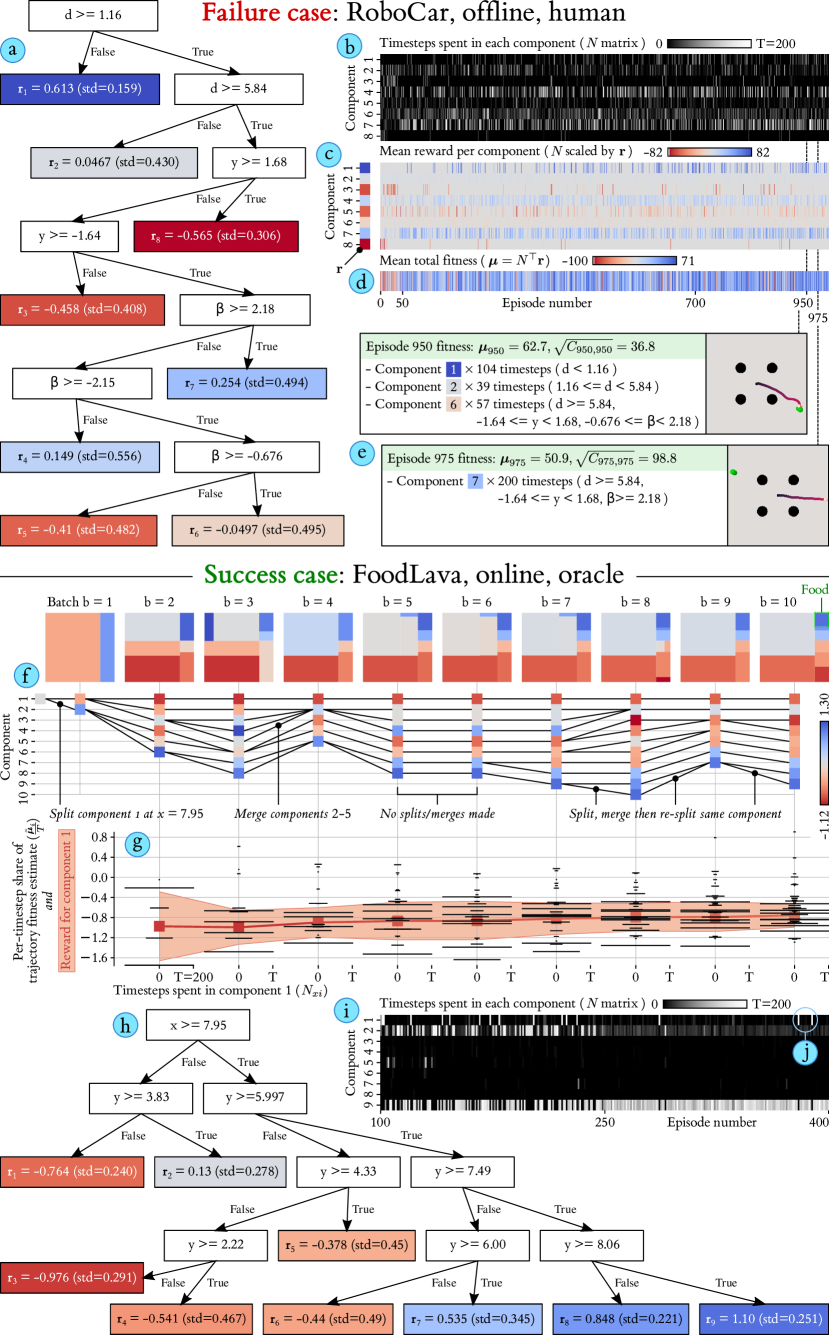
Figure 6. Interpretability demo for two exemplar cases.

7. Conclusion

We have presented an algorithm for interpretable PbRL using tree-structured reward functions, demonstrating successful learning of compact and aligned reward functions across four environments, alongside informative and actionable failure cases due to causal confusion in the offline setting and premature reward fixing in the online setting. We have also shown the value of interpretability for exploring and debugging the learnt reward structure. In the offline setting, future work could construct trajectory datasets using unsupervised agents that optimise for behavioural diversity (e.g. Eysenbach et al. (2018)) instead of our somewhat contrived pilot agents. In the online setting, there is scope for larger human experiments, with a focus on ablation and hyperparameter tuning. An additional layer of interpretability could be realised by integrating our method with agent architectures that learn decomposed value functions Juozapaitis et al. (2019).

See pages - of appendix

References

- (1)
- Abbeel and Ng (2004) Pieter Abbeel and Andrew Y Ng. 2004. Apprenticeship learning via inverse reinforcement learning. In Proceedings of the twenty-first international conference on Machine learning. 1.
- Akrour et al. (2012) Riad Akrour, Marc Schoenauer, and Michèle Sebag. 2012. April: Active preference learning-based reinforcement learning. In Joint European Conference on Machine Learning and Knowledge Discovery in Databases. Springer, 116–131.
- Arzate Cruz and Igarashi (2020) Christian Arzate Cruz and Takeo Igarashi. 2020. A survey on interactive reinforcement learning: Design principles and open challenges. In Proceedings of the 2020 ACM Designing Interactive Systems Conference. 1195–1209.
- Bewley and Lawry (2021) Tom Bewley and Jonathan Lawry. 2021. TripleTree: A Versatile Interpretable Representation of Black Box Agents and their Environments. In Proceedings of the AAAI Conference on Artificial Intelligence, Vol. 35. 11415–11422.
- Bradley and Terry (1952) Ralph Allan Bradley and Milton E Terry. 1952. Rank analysis of incomplete block designs: I. The method of paired comparisons. Biometrika 39, 3/4 (1952), 324–345.
- Breiman et al. (2017) Leo Breiman, Jerome H Friedman, Richard A Olshen, and Charles J Stone. 2017. Classification and regression trees. Routledge.
- Carpentier et al. (2011) Alexandra Carpentier, Alessandro Lazaric, Mohammad Ghavamzadeh, Rémi Munos, and Peter Auer. 2011. Upper-confidence-bound algorithms for active learning in multi-armed bandits. In International Conference on Algorithmic Learning Theory. Springer, 189–203.
- Christiano et al. (2017) Paul F Christiano, Jan Leike, Tom Brown, Miljan Martic, Shane Legg, and Dario Amodei. 2017. Deep Reinforcement Learning from Human Preferences. In Advances in Neural Information Processing Systems, I. Guyon, U. V. Luxburg, S. Bengio, H. Wallach, R. Fergus, S. Vishwanathan, and R. Garnett (Eds.), Vol. 30.
- Csató (2015) László Csató. 2015. A graph interpretation of the least squares ranking method. Social Choice and Welfare 44, 1 (2015), 51–69.
- Dewey (2014) Daniel Dewey. 2014. Reinforcement learning and the reward engineering principle. In 2014 AAAI Spring Symposium Series.
- Eysenbach et al. (2018) Benjamin Eysenbach, Abhishek Gupta, Julian Ibarz, and Sergey Levine. 2018. Diversity is all you need: Learning skills without a reward function. arXiv preprint arXiv:1802.06070 (2018).
- Fujimoto et al. (2018) Scott Fujimoto, Herke Hoof, and David Meger. 2018. Addressing function approximation error in actor-critic methods. In International Conference on Machine Learning. PMLR, 1587–1596.
- Gulliksen (1956) Harold Gulliksen. 1956. A least squares solution for paired comparisons with incomplete data. Psychometrika 21, 2 (1956), 125–134.
- Guo et al. (2018) Yuan Guo, Peng Tian, Jayashree Kalpathy-Cramer, Susan Ostmo, J Peter Campbell, Michael F Chiang, Deniz Erdogmus, Jennifer G Dy, and Stratis Ioannidis. 2018. Experimental Design under the Bradley-Terry Model.. In IJCAI. 2198–2204.
- Hadfield-Menell et al. (2017) Dylan Hadfield-Menell, Smitha Milli, Pieter Abbeel, Stuart J Russell, and Anca Dragan. 2017. Inverse Reward Design. In Advances in Neural Information Processing Systems, I. Guyon, U. V. Luxburg, S. Bengio, H. Wallach, R. Fergus, S. Vishwanathan, and R. Garnett (Eds.), Vol. 30. Curran Associates, Inc. https://proceedings.neurips.cc/paper/2017/file/32fdab6559cdfa4f167f8c31b9199643-Paper.pdf
- Ibarz et al. (2018) Borja Ibarz, Jan Leike, Tobias Pohlen, Geoffrey Irving, Shane Legg, and Dario Amodei. 2018. Reward learning from human preferences and demonstrations in Atari. In Advances in Neural Information Processing Systems, S. Bengio, H. Wallach, H. Larochelle, K. Grauman, N. Cesa-Bianchi, and R. Garnett (Eds.), Vol. 31.
- Jauhri et al. (2020) Snehal Jauhri, Carlos Celemin, and Jens Kober. 2020. Interactive Imitation Learning in State-Space. In Conference on Robot Learning.
- Juozapaitis et al. (2019) Zoe Juozapaitis, Anurag Koul, Alan Fern, Martin Erwig, and Finale Doshi-Velez. 2019. Explainable reinforcement learning via reward decomposition. In IJCAI/ECAI Workshop on Explainable Artificial Intelligence.
- Leike et al. (2018) Jan Leike, David Krueger, Tom Everitt, Miljan Martic, Vishal Maini, and Shane Legg. 2018. Scalable agent alignment via reward modeling: a research direction. arXiv preprint arXiv:1811.07871 (2018).
- Maclin and Shavlik (1996) Richard Maclin and Jude W Shavlik. 1996. Creating advice-taking reinforcement learners. Machine Learning 22, 1 (1996), 251–281.
- Michaud et al. (2020) Eric J Michaud, Adam Gleave, and Stuart Russell. 2020. Understanding learned reward functions. arXiv preprint arXiv:2012.05862 (2020).
- Mosteller (1951) Frederick Mosteller. 1951. Remarks on the method of paired comparisons: I. The least squares solution assuming equal standard deviations and equal correlations. Psychometrika 16, 1 (1951), 3–9.
- Russell and Santos (2019) Jacob Russell and Eugene Santos. 2019. Explaining reward functions in markov decision processes. In The Thirty-Second International Flairs Conference.
- Silver et al. (2021) David Silver, Satinder Singh, Doina Precup, and Richard S Sutton. 2021. Reward is enough. Artificial Intelligence (2021), 103535.
- Singh et al. (2009) Satinder Singh, Richard L Lewis, and Andrew G Barto. 2009. Where do rewards come from?. In Proceedings of the annual conference of the cognitive science society. Cognitive Science Society, 2601–2606.
- Talati et al. (2021) Aditi Talati, Dorsa Sadigh, et al. 2021. APReL: A Library for Active Preference-based Reward Learning Algorithms. arXiv preprint arXiv:2108.07259 (2021).
- Thurstone (1927) Louis L Thurstone. 1927. A law of comparative judgment. Psychological review 34, 4 (1927), 273.
- Wirth et al. (2017) Christian Wirth, Riad Akrour, Gerhard Neumann, Johannes Fürnkranz, et al. 2017. A survey of preference-based reinforcement learning methods. Journal of Machine Learning Research 18, 136 (2017), 1–46.
- Xu et al. (2020) Yichong Xu, Ruosong Wang, Lin Yang, Aarti Singh, and Artur Dubrawski. 2020. Preference-based Reinforcement Learning with Finite-Time Guarantees. Advances in Neural Information Processing Systems 33 (2020).
- Zoghi et al. (2014) Masrour Zoghi, Shimon Whiteson, Remi Munos, and Maarten Rijke. 2014. Relative upper confidence bound for the k-armed dueling bandit problem. In International conference on machine learning. PMLR, 10–18.