New Formulas for the Euler-Mascheroni Constant and other
Consequences derived from the Acceptance of Hyperbolicity of Jensen
Polynomials and the Analysis of the Turán Moments for the $\xi$-Function

Research Content

The Euler-Mascheroni constant is calculated by three novel representations over these sets respectively: 1) Turán moments, 2) coefficients of Jensen polynomials for the Taylor series of the Riemann Xi function at $s=1/2+i.t$ and 3) even coefficients of the Riemann Xi function around $s=1/2$. These findings support the acceptance of the property of hyperbolicity of Jensen polynomials within the scope of the Riemann Hypothesis due to exactness on the approximations calculated not only for the Euler-Mascheroni constant, but also for the Bernoulli numbers and the even derivatives of the Riemann Xi function at $s=1/2$. The new formulas are linked to similar patterns observed in the formulation of the Akiyama-Tanigawa algorithm based on the Gregory coefficients of second order and lead to understanding the Riemann zeta function as a bridge between the Gregory coefficients and other relevant sets

Abstract

We calculate the Euler-Mascheroni constant $\gamma$ in this article by a convergent series that requires the computation of few Turán moments $\widehat{b}_{n}$ or their equivalent definition in terms of the coefficients $c_{n}$ of the Jensen polynomials $J^{d,N}(x)$ of degree $d$ and shift $N=0$ for the Taylor series of the Riemann $\xi$-function at the special points $s=\frac{x}{2}$ and $s=\frac{1}{2}+ix$. This fascinating result comes from the consequences of the explicit multiplication of all the factors with each other indicated by the Hadamard product of the $\xi$-function at the complex variable $s$, which leads to write a convenient algebraic expansion in $s^{0},s^{1},s^{2},s^{3}\ldots$ that can be plausibly compared to the equivalent terms in $s^{0},s^{1},s^{2},s^{3}\ldots$ derived from the Taylor series for the $\xi$-function around $\frac{1}{2}$, i.e., the Taylor series and Hadamard product of $\xi$ must be equivalents to each other because they represent the Riemann $\xi$ function. Hence, new priceless summation formulas that support the novel representations for $\gamma$ are presented in this article leading to relate successfully the coefficients of the Taylor series for the $\xi$ function to the non-trivial zeros of the Riemann zeta function $\zeta$ and the well-known values $\Gamma\left(\frac{1}{4}\right),\zeta\left(\frac{1}{2}\right),\gamma$ and the Lugo’s constant within this scope. Furthermore, it is provided a thorough inspection of the numerical results for the first twenty-one values of $c_{n}$ and $\widehat{b}_{n}$, for $n=$ $0,1,2\ldots,20$, and their role in the representations proposed for $\gamma$, which would support the formulation of all the $c_{n}$ and $\widehat{b_{n}}$ and their connection with the even derivatives of $\xi$ at $s=\frac{1}{2}$. As an important conclusion of this work, the new representations for the Euler-Mascheroni constant could be significant consequences of the Riemann Hypothesis due to the tremendous precision and assertiveness achieved for $\gamma$ based on that hypothesis

Keywords: Euler-Mascheroni constant, coefficients of Jensen polynomials, Turán Moments, Riemann Xi-function, Riemann zeta function, non-trivial zeros of the Riemann zeta function, Riemann Hypothesis, Hadamard product, Taylor series, even derivatives of the Xi-function, Lugo constant, Gregory coefficients, Akiyama-Tanigawa’s formula, hyperbolicity, Bernoulli numbers

I. Introduction

We have deduced a new formula for the Euler-Mascheroni constant $\gamma$ based on the set of the Turán moments $\widehat{b}_{n}$ whose role could be crucial for the analysis of the Riemann Hypothesis. Hence,

$$\gamma=\log(4\pi)-2+\left(2^{7}\right)\sum_{n=1}^{\infty}\frac{n\widehat{b}_{n}}{(2n)!}.$$

That formula could be reinforcing potential consequences derived from the validation of the property known as hyperbolicity of the Jensen polynomials for a particular Taylor series for the Riemann Xi function at $s=\frac{1}{2}+i.x$. Thus, we provide a clear evidence that the real roots $x$ defined by the assumption of hyperbolicity of the Jensen polynomials $J^{d,N}(x)$ necessarily lead to link the expected coefficients $\widehat{b}_{n},c_{n}$ and $a_{2n}$ with each other as discussed in this article, which would support significantly the Riemann Hypothesis itself because these coefficients $\widehat{b_{n}},a_{2n}$ and $c_{n}$ cannot be casually computed without assuming that major Conjecture on the structure of the roots $s=\frac{1}{2}+i.x$ within the Hadamard product and Taylor series for the Riemann Xi function as explained later. We offer numerical data by the use of already computed Turán moments $\widehat{b}_{n}$ replaced in the new formula for $\gamma$, but also by the summation series involving the even-index coefficients $a_{2n}$ that will be discussed thoroughly later. Thus, the second version for the EulerMascheroni constant we dealt with in this article is given by

$$\gamma=\log(4\pi)-2+\left(2^{4}\right)\sum_{n=1}^{\infty}\frac{na_{2n}}{2^{2n}}.$$

Then, we will revise later that the coefficients $a_{2n}$ are related to the Turán moments $\widehat{b}_{n}$ by the relation

$$a_{2n}=\frac{2^{3}\left(2^{2n}\right)\widehat{b}_{n}}{(2n)!}=\frac{8\cdot\left(2^{2n}\right)\widehat{b}_{n}}{(2n)!},$$

and thanks to a rigorous experimental inspection, we have concluded that the $c_{n}$ are linked to the other coefficients $a_{2n}$ and $\widehat{b}_{n}$ as follows

$$c_{n}=2(n!)(-1)^{n}a_{2n}=(-1)^{n}\frac{n!}{(2n)!}2^{2n}\cdot 2^{4}\cdot\widehat{b}_{n}$$

Therefore, we have found that a third formula for the Euler-Mascheroni constant is defined by the coefficients $c_{n}$ of the Jensen polynomials within our approach as

$$\gamma=\log(4\pi)-2+\left(2^{3}\right)\sum_{n=1}^{\infty}\frac{n(-1)^{n}c_{n}}{\left(2^{2n}\right)n!}$$

As a result, the previous three formulas for the Euler-Mascheroni constant and the precise ways to link the coefficients $c_{n},a_{2n}$ and $\widehat{b}_{n}$ with each other are the main set of unpublished findings for this important constant we offer in our research work. Furthermore, we provide strict numerical evaluation for the approximation for the Euler-Mascheroni constant, which can be easily calculated by anyone using the data we present for the $c_{n},a_{2n}$ and $\widehat{b}_{n}$ in the Table 1 , just replacing these coefficients as follows

Version 1, using the $\widehat{b}_{n}$ of Table 1:

$$\gamma=\log(4\pi) -2+\left(2^{7}\right)\sum_{n=1}^{\infty}\frac{n\widehat{b}_{n}}{(2n)!}\approx 0.53102424697+\left(2^{7}\right)\left(\frac{\widehat{b}_{1}}{2!}+\frac{2\widehat{b}_{2}}{4!}+\cdots+20\frac{\widehat{b}_{20}}{40!}\right)\approx$$

$$\approx 0.53102424697+\left(2^{7}\right)\left(3.60870452595\left(10^{-4}\right)\right)\approx 0.577215664902.$$

Version 2, using the $a_{2n}$ of Table 1:

$$\gamma=\log(4\pi) -2+\left(2^{4}\right)\sum_{n=1}^{\infty}\frac{na_{2n}}{2^{2n}}\approx 0.53102424697+16\left(\frac{a_{2}}{4}+\frac{2a_{4}}{16}+\cdots+\frac{20a_{40}}{2^{40}}\right)\approx$$

$$\approx 0.577215664902,$$

Version 3, using the $c_{n}$ of Table 1:

$$\gamma\approx 0.53102424697+\left(2^{3}\right)\left(\frac{-c_{1}}{4}+\frac{2c_{2}}{16(2!)}-\cdots+\frac{20c_{20}}{2^{40}(20!)}\right)\approx 0.577215664902.$$

The previous representations are consistent and look similar to other known formulas like the Akiyama-Tanigawa’s representation, which involves an interesting pattern below

$$\gamma=\log(2\pi)-2-2\sum_{n=1}^{\infty}\frac{(-1)^{n}G_{n}(2)}{n}.$$

We have noticed that the structure of this formula, although over the numbers $G_{n}(2)$ known as the Gregory coefficients of the second order, is extremely similar, but not the same, to our cases based on the $c_{n},a_{2n}$ and $\widehat{b_{n}}$ which is not a coincidence because our novel representations for the Euler-Mascheroni constant have been inferred from a new totally different approach which is independent of the Akiyama-Tanigawa’s formulation. Furthermore, other findings or discoveries introduced here are one summation formula that involves the non-trivial zeros $s_{r}=\sigma_{r}+t_{r}.i$ and $\bar{s}_{r}=\sigma_{r}-t_{r}.i$ of the Riemann zeta function to the coefficients $a_{2n}$ given by:

$$\sum_{r=1}^{\infty}\frac{\sigma_{r}}{s_{r}\bar{s}_{r}}=\left(\frac{4a_{2}}{2^{2}}+\frac{4(2)a_{4}}{2^{4}}+\frac{4(3)a_{6}}{2^{6}}+\frac{4(4)a_{8}}{2^{8}}+\cdots\right)=\sum_{n=1}^{\infty}\frac{4na_{2n}}{2^{2n}},$$

and a second summation relating the coefficients $a_{2n}$ as well:

$$\frac{1}{2}=\left(\frac{a_{0}}{2^{0}}+\frac{a_{2}}{2^{2}}+\frac{a_{4}}{2^{4}}+\frac{a_{6}}{2^{6}}+\cdots\right)=\sum_{n=0}^{\infty}\frac{a_{2n}}{2^{2n}}.$$

We will discuss later that these last results really are reduced to the following expressions

$$\sum_{r=1}^{\infty}\frac{\frac{1}{2}}{s_{r}\bar{s}_{r}}=\frac{1}{2}\sum_{r=1}^{\infty}\frac{1}{\left(\frac{1}{2}+t_{r}\cdot i\right)\left(\frac{1}{2}-t_{r}\cdot i\right)}=\sum_{n=1}^{\infty}\frac{4na_{2n}}{2^{2n}},$$

and

$$\sum_{n=0}^{\infty}\frac{a_{2n}}{2^{2n}}=\frac{1}{2},$$

because the numerical evidence of the computed coefficients demands obligatorily the acceptance of the real part as strictly $\sigma_{r}=\frac{1}{2}$ for every non-trivial zero of the Riemann Zeta function. All these results will be explained carefully by our approach of equating the Hadamard product and Taylor series for the Riemann Xi function. For now, we introduce the crucial formulas that can be checked simply by replacing the data of the Table 1 as revised later.

We have also discovered another expected pattern to calculate the Bernoulli numbers $B_{2r}$, whose index $2r$ is considered for $r=0,1,2\ldots$, which leads to involve the coefficients $\widehat{b}_{n}$ and $c_{n}$ after having assumed the complete property of hyperbolicity of the Jensen polynomials for the Taylor series of the Riemann Xi function. We compute successfully various values of $B_{2r}$ by using the valid coefficients of the Jensen polynomials, i.e., the coefficients $c_{n}$ are achievable as expected by the acceptance of the property of hyperbolicity and the unique real part $\frac{1}{2}$ for the formulations of the non-trivial zeros $s_{r}=\frac{1}{2}+t_{r}.i$. The formulas for the Bernoulli numbers $B_{2r}$ deduced here are

$$B_{2r}=\frac{16(-1)^{r-1}\cdot(2r)!2^{-2r}}{(\pi)^{r}(2r-1)\mathrm{r}!}\sum_{n=0}^{\infty}\frac{2^{2n}\widehat{b}_{\mathrm{n}}\left(2r-\frac{1}{2}\right)^{2n}}{(2n)!},$$

$$B_{2r}=\frac{(-1)^{r-1}\cdot(2r)!2^{1-2r}}{(\pi)^{r}(2r-1)\mathrm{r}!}\sum_{n=0}^{\infty}\frac{(-1)^{n}c_{n}\left(2r-\frac{1}{2}\right)^{2n}}{2(n)!},$$

of course, by replacing $c_{n}=2(n!)(-1)^{n}a_{2n}$, we could find a third formula based on these coefficients $a_{2n}$, thus, if someone wants to compute particular Bernoulli numbers based on the Turán moments $\widehat{b}_{n}$ or also by the coefficients $c_{n}$ of the Jensen polynomials, or even index coefficients $a_{2n}$ could use the Table 1 with twenty-one data of these coefficients in order to verify it. As reinforce of our approach, if these coefficients $a_{2n},c_{n}$ and $\widehat{b}_{n}$ had not been properly calculated, then, neither the Bernoulli numbers nor the even derivatives of the Riemann Xi function at $s=1/2$ and all the formulations for the Euler-Mascheroni constant never had been achievable! Hence, the validity of all the non-trivial zeros with real part $\frac{1}{2}$ is clear as stated on the Riemann Hypothesis.

Regarding the relevance of these results, we propose in the current introduction that findings about new links between the Euler-Mascheroni constant $\gamma=0.57721\ldots$ and other important numbers in mathematics could help to unravel fundamental conjectures with extraordinary consequences in several fields of exact sciences and industrial technologies. We propose the use of these less known coefficients $a_{2n},c_{n}$ and $\widehat{b}_{n}$ as very important set of numbers within the study of other famous sets like the Gregory coefficients of higher orders. As a result, we define the Gregory coefficients $G_{n}=G_{n}(1),n\geq 2$, with basic order 1, by a well-known expression like

$$G_{n}=-\frac{B_{n}{}^{(n-1)}}{(n-1)\cdot(n!)}$$

which introduces immediately a new relationship between $G_{2r}=G_{2r}(1)$ and the respective $c_{n}$, $a_{2n}$ and $\widehat{b_{n}}$ because we already know that we can replace the previous formula in the proposed ones for $B_{2r}$

$$B_{2r}=\frac{16(-1)^{r-1}\cdot(2r)!2^{-2r}}{(\pi)^{r}(2r-1)r!}\sum_{n=0}^{\infty}\frac{2^{2n}\widehat{b}_{\mathrm{n}}\left(2r-\frac{1}{2}\right)^{2n}}{(2n)!}=\sqrt[2r-1]{-G_{2r}(2r-1)\cdot(2r)!}$$

$$B_{2r}=\frac{(-1)^{r-1}\cdot(2r)!2^{1-2r}}{(\pi)^{r}(2r-1)r!}\sum_{n=0}^{\infty}\frac{(-1)^{n}c_{n}\left(2r-\frac{1}{2}\right)^{2n}}{2(n)!}=\sqrt[2r-1]{-G_{2r}(2r-1)\cdot(2r)!}$$

which lead to formulate the Gregory coefficients $G_{2r}$ in function of the either $c_{n}$ or $\widehat{b}_{n}$, with possibility of expressing $G_{2r}$ in terms of $a_{2n}$ as well. So the vital numbers $c_{n},\widehat{b_{n}}$ and $a_{2n}$ can act as generators of the fundamental numbers $B_{2r}$ of Bernoulli or the Gregory of type $G_{2r}$. These are perhaps the greatest conclusions derived in this article as nobody had noticed such numerical findings.

We also want to introduce some famous definitions for $\gamma$ that every reader of the article needs to assimilate in order to understand that our formulas are not the only ones, there are many others, e.g., the limit based on the Harmonic numbers [1] $H_{n}=\sum\limits_{k=1}^{n}\frac{1}{k}$, being $\log n$ the natural logarithm of $n$ or $\ln(n)$

$$\gamma=\lim_{n\rightarrow\infty}\left(H_{n}-\log n\right),$$

which is given by the convergent series

$$\gamma=\sum_{n=2}^{\infty}(-1)^{n}\frac{\zeta(n)}{n},$$

whose definition over the terms $\zeta(n)$, for $n=2,3,4\ldots$, draws attention due to the relevance of the Riemann zeta function in number theory and functional analysis. Furthermore, the beautiful expression

$$\sum_{\rho}\frac{1}{\rho}=1+\frac{\gamma}{2}-\frac{\log(4\pi)}{2},$$

defines a summation over the inverses of all the values $\rho=s_{r}$ or $\rho=\bar{s}_{r}$ known as the non-trivial zeros of the Riemann zeta function, being $s_{r}=\sigma_{r}+it_{r}$ and $\bar{s}_{r}=\sigma_{r}-it_{r}$, where a useful count index $r=1,2,3,\ldots$ lets distinguish the different zeros $s_{1},s_{2},s_{3},\ldots\bar{s}_{1},\bar{s}_{2},\bar{s}_{3},\ldots$ from each other. In this regard, one of the most important unsolved problems in mathematics is related to the nature of the real part of these $\rho$, i.e., for each $\sigma_{r}$, since all the calculations made so far have not been able to yield a non-trivial zero of the Riemann zeta function that had a real part different from $\frac{1}{2}$, e.g., $\sigma_{1}=\frac{2}{3},\sigma_{2}=\frac{3}{5},\ldots$ or others. In this article is discussed an approach that links not only the Eq.(3) to the non-trivial zeros $\rho$, but also to the coefficients $a_{2n}$ [2] of the Taylor series for the Riemann $\xi$ function, around the point $s_{0}=\frac{1}{2}$, given by

$$\xi(s)=\sum_{n=0}^{\infty}a_{2n}\left(s-s_{0}\right)^{2n}=\sum_{n=0}^{\infty}a_{2n}\left(s-\frac{1}{2}\right)^{2n}.$$

Then, a summation involving each $a_{2n}$, or later, each Jensen $c_{n}$ (or also the Turán moments $\widehat{b_{n}}$ or indistinctly $\widehat{b}_{m}$ ), would lead to calculate the Euler-Mascheroni constant with high fidelity.

In the references about the Riemann $\xi$-function, the first coefficient $a_{0}=-\frac{\Gamma\left(\frac{1}{4}\right)\left(\frac{1}{2}\right)}{8\pi^{\frac{1}{4}}}=$ $0.497120\ldots[3]$ is exactly formulated thanks to the calculation of the integral

$$a_{2n}=4\int_{1}^{\infty}\frac{d\left[x^{\frac{3}{2}}\psi^{\prime}(x)\right]}{dx}\frac{\left(\frac{1}{2}\ln x\right)^{2n}}{(2n)!}x^{-\frac{1}{4}}dx,$$

at $n=0$, where $a_{2(0)}=a_{0}$ and $\psi(x)=\sum\limits_{m=1}^{\infty}e^{-m^{2}\pi x}=\frac{1}{2}\left[\vartheta_{3}\left(0,e^{-\pi x}\right)-1\right]$, being $\vartheta_{3}$ the Jacobi theta function. Moreover, $A_{0}=a_{0}=\frac{\left.d^{(0)}\xi\left(\frac{1}{2}+ix\right)\right|_{x=0}}{dx^{(0)}}=-\frac{\Gamma\left(\frac{1}{4}\right)\zeta\left(\frac{1}{2}\right)}{8\pi^{\frac{1}{4}}}$ which can be inferred from the representation given by DeFranco [4] in the following Taylor series for $\xi(s)$, at $s=\frac{1}{2}+ix$, with $x$ a real number

$$\xi\left(\frac{1}{2}+ix\right)=\sum_{n=0}^{\infty}(-1)^{n}A_{n}x^{2n}=\sum_{n=0}^{\infty}(-1)^{n}a_{2n}x^{2n},$$

being $A_{n}=a_{2n}=\left.\frac{(-1)^{2n}}{(2n)!}\frac{d^{2n}}{d^{2n}x}\xi\left(\frac{1}{2}+ix\right)\right|_{x=0}$. Therefore, each $a_{2n}$ would require very complicated steps of evaluation which could limit apparently a complete representation for the Riemann $\xi$ function through the computation of thousands of such coefficients. However, in this article is argued that, in fact, each $a_{2n}$ can be analytically and numerically represented by the coefficients $c_{n}$ of the Jensen polynomials $J^{d,N}(x)$ of degree $d$ and shift $N=0$ for the Taylor series of the Riemann $\xi$-function or, instead, the little known Turán moments $\widehat{b}_{n}$ which were already tabulated almost three decades ago!, e.g., the first twenty-one data found in [5]. Furthermore, each $c_{n}$ can be calculated by special summation series, corroborated by the even derivatives of the Riemann $\xi$ function at $\frac{1}{2}$, that involve the computation of all the non-trivial zeros $\rho$ but only if the assertion of the Riemann Hypothesis was accepted, i.e., $\sigma_{r}=\frac{1}{2}$ for $r=1,2,3,\ldots$, as clearly exposed in this work. In fact, with a few tens of $c_{n}$ (and some thousands of non-trivial zeros $s_{r}=\sigma_{r}+it_{r}$, assuming $\sigma_{r}=\frac{1}{2}$ ) it would be possible to achieve numerically a good representation for the EulerMascheroni constant according to the approach introduced in this article, which is proved computationally with extraordinary effectiveness. As a result, each $A_{n}$ or $a_{2n}$ is exactly defined in terms of the $c_{n}$, and later, $\gamma$ will have a representation based on those values as well. Throughout this article, the assumption of the Riemann Hypothesis plays an important role because it leads to raise consequences never seen before that let refine the model of the Taylor series for Eq.(4) and Eq.(6), and other results explained later. Nevertheless, in the proposed methodology, there will be made clear that the Riemann Hypothesis has not to be neither assumed nor proved in order to equate the representation for the Hadamard product of the Riemann $\xi$-function to the Taylor series in Eq.(4). In this regard, the most fascinating scenario for future research is the deduction of not just one, not two, but thousands of formulations relating the $a_{2n},c_{n}$ and $\widehat{b}_{n}$ to various sequences based on the non-trivial zeros of the Riemann zeta function that would be the result of the natural comparison between the Hadamard product of the $\xi$-function and its Taylor series.


Theory

Based on the Taylor series given by Eq.(4) and the representation for the Hadamard product of the Riemann $\xi$-function [6]

$$\xi(s)=\frac{1}{2}\prod_{\rho}\left(1-\frac{s}{\rho}\right),$$

being $\rho=s_{r}$ or also $\rho=\bar{s}_{r}$ all the non-trivial zeros of the Riemann zeta function, i.e., including all the conjugate pairs $s_{r}=\sigma_{r}+it_{r}$ and $\bar{s}_{r}=\sigma_{r}-it_{r}$, then, Eq.(7) can be conveniently adapted to the algebraic equivalent version deduced by professor Alhargan [7] and published few months ago

$$\xi(s)=\frac{1}{2}\prod_{\rho}\left(1-\frac{s}{\rho}\right)=\frac{1}{2}\prod_{r=1}^{\infty}\left(1-\frac{s\left(2\sigma_{r}-s\right)}{s_{r}\bar{s}_{r}}\right),$$

being $\sigma_{r}$ the real part of the non-trivial zeros of the Riemann zeta function. At this point, it is important to clarify that Eq.(4) and Eq.(8) are absolutely equivalent to each other because both of them represent the same function, i.e., the Riemann $\xi$-function. Therefore, the Hadamard product is developed on the right side of Eq.(9), with the $\frac{1}{2}$ being algebraically included only in the first factor, as follows

$$\sum_{n=0}^{\infty}a_{2n}\left(s-\frac{1}{2}\right)^{2n}=\left[\frac{1}{2}-\frac{s\left(2\sigma_{1}-s\right)}{2s_{1}\bar{s}_{1}}\right]\left[1-\frac{s\left(2\sigma_{2}-s\right)}{s_{2}\bar{s}_{2}}\right]\left[1-\frac{s\left(2\sigma_{3}-s\right)}{s_{3}\bar{s}_{3}}\right]\left[1-\frac{s\left(2\sigma_{4}-s\right)}{s_{4}\bar{s}_{4}}\right]\ldots$$

Then, after the product of the first two factors $\left[\frac{1}{2}-\frac{s\left(2\sigma_{1}-s\right)}{2s_{1}\bar{s}_{1}}\right],\left[1-\frac{s\left(2\sigma_{2}-s\right)}{s_{2}\bar{s}_{2}}\right]$ to each other

$$\sum_{n=0}^{\infty}a_{2n}\left(s-\frac{1}{2}\right)^{2n}=$$

$$=\left[\frac{1}{2}-\frac{s\left(2\sigma_{2}-s\right)}{2s_{2}\bar{s}_{2}}-\frac{s\left(2\sigma_{1}-s\right)}{2s_{1}\bar{s}_{1}}+\frac{s^{2}\left(2\sigma_{1}-s\right)\left(2\sigma_{2}-s\right)}{2s_{1}\bar{s}_{1}s_{2}\bar{s}_{2}}\right]\left[1-\frac{s\left(2\sigma_{3}-s\right)}{s_{3}\bar{s}_{3}}\right]\left[1-\frac{s\left(2\sigma_{4}-s\right)}{s_{4}\bar{s}_{4}}\right]\ldots,$$

and when multiplying carefully more and more factors with each other and rearranging the long results, a noticeable pattern begins to emerge, mainly for $s^{0}$ and $s^{1}$, which undoubtedly defines the coefficients that accompany the terms $s^{0},s^{1},s^{2},s^{3}\ldots$ on the right side of the Eq.(9) as follows

$$\sum_{n=0}^{\infty}a_{2n}\left(s-\frac{1}{2}\right)^{2n}=\frac{1}{2}s^{0}-\left(\frac{\sigma_{1}}{s_{1}\bar{s}_{1}}+\frac{\sigma_{2}}{s_{2}\bar{s}_{2}}+\frac{\sigma_{3}}{s_{3}\bar{s}_{3}}+\cdots\right)s^{1}+\left(\frac{1}{2s_{1}\bar{s}_{1}\ldots}+\frac{1}{2s_{2}\bar{s}_{2}\ldots}+\frac{1}{2s_{3}\bar{s}_{3}\ldots}+\right.$$

$$\left.+\frac{2\sigma_{1}\sigma_{2}\ldots}{s_{1}\bar{s}_{1}s_{2}\bar{s}_{2}\ldots}+\cdots\right)s^{2}+\left(-\frac{\sigma_{1}\ldots}{s_{1}\bar{s}_{1}s_{2}\bar{s}_{2}\ldots}-\cdots\right)s^{3}+\cdots+F_{j}s^{j}+F_{j+1}s^{j+1}+\cdots,$$

where the coefficients with more complexity in Eq.(11), such like those for $s^{2},s^{3},\ldots,s^{j},s^{j+1},\ldots$, and successive expressions, have been indicated implicitly, with some parts in ellipsis and denominations like $F_{j},F_{j+1}$, as they are not going to be used in the calculation of the EulerMascheroni constant. However, they could play a relevant role to broaden this research in the future, being necessary to define them in new quests of results. Then, the Eq.(11) can be written as

$$\sum_{n=0}^{\infty}a_{2n}\left(s-\frac{1}{2}\right)^{2n}=\frac{1}{2}s^{0}-\left(\sum_{r=1}^{\infty}\frac{\sigma_{r}}{s_{r}\bar{s}_{r}}\right)s^{1}+F_{2}s^{2}+F_{3}s^{3}+\cdots+F_{j}s^{j}+F_{j+1}s^{j+1}+\cdots,$$

being the coefficients $F_{0}=\frac{1}{2},F_{1}=-\sum\limits_{r=1}^{\infty}\frac{\sigma_{r}}{s_{r}\bar{s}_{r}},F_{2}=\frac{1}{2s_{1}\bar{s}_{1}\ldots}+\frac{1}{2s_{2}\bar{s}_{2}\ldots}+\cdots,F_{3}=-\frac{\sigma_{1}\ldots}{s_{1}\bar{s}_{1}s_{2}\bar{s}_{2}\ldots}-\cdots$, and the successive undefined terms like $F_{j}$ and $F_{j+1}$ for future advances.

Now, the expansion of the left side of Eq.(11) or Eq.(12), up to certain organized arrangement for the terms $s^{0},s^{1},s^{2},s^{3}$, leads to understand clearly why the Hadamard product of the Riemann $\xi$-function corresponds exactly to the Taylor series for the same function. First, the pattern of the summation in the left side of Eq.(12) is tentatively developed according to the first addends given by $a_{0}\left(s-\frac{1}{2}\right)^{0},a_{2}\left(s-\frac{1}{2}\right)^{2},a_{4}\left(s-\frac{1}{2}\right)^{4}$ $\ldots$ for the indicated power exponent $2n$. This approach represents an intuitive operation that can be validated algebraically and whose consistency will be proved thanks to the truthful formulas obtained in this article and introduced before. Therefore, the left side of Eq.(12) is expanded as follows

$$\sum_{n=0}^{\infty}a_{2n}\left(s-\frac{1}{2}\right)^{2n}=a_{0}\left(s-\frac{1}{2}\right)^{0}+a_{2}\left(s-\frac{1}{2}\right)^{2}+ a_{4}\left(s-\frac{1}{2}\right)^{4}\ldots=a_{0}+a_{2}\left(s^{2}-s+\frac{1}{4}\right)+$$

$$+a_{4}\left(s^{2}-s+\frac{1}{4}\right)\left(s^{2}-s+\frac{1}{4}\right)+\cdots$$

and after a careful factorization of the expressions based on the coefficients $a_{2n}$ in Eq.(13)

$$\sum_{n=0}^{\infty}a_{2n}\left(s-\frac{1}{2}\right)^{2n} =\left(\frac{a_{0}}{2^{0}}+\frac{a_{2}}{2^{2}}+\frac{a_{4}}{2^{4}}+\frac{a_{6}}{2^{6}}+\cdots\right)s^{0}+\left(-\frac{4a_{2}}{2^{2}}-\frac{4(2)a_{4}}{2^{4}}-\frac{4(3)a_{6}}{2^{6}}-\frac{4(4)a_{8}}{2^{8}}-\cdots\right)s^{1}+$$

$$+G_{2}s^{2}+G_{3}s^{3}+\cdots+G_{j}s^{j}+G_{j+1}s^{j+1}+\cdots$$

where $G_{0}=\left(\frac{a_{0}}{2^{0}}+\frac{a_{2}}{2^{2}}+\frac{a_{4}}{2^{4}}+\frac{a_{6}}{2^{6}}+\cdots\right),G_{1}=\left(-\frac{4a_{2}}{2^{2}}-\frac{4(2)a_{4}}{2^{4}}-\frac{4(3)a_{6}}{2^{6}}-\frac{4(4)a_{8}}{2^{8}}-\cdots\right)$ and the others coefficients in Eq.(14) would be represented by $G_{2},G_{3},\ldots,G_{j},G_{j+1},\ldots.$ Therefore, every coefficient indicated by the letter $G$ could be compared to the equivalent counterpart $F$ as follows

$$F_{0}=\frac{1}{2}=G_{0}=\left(\frac{a_{0}}{2^{0}}+\frac{a_{2}}{2^{2}}+\frac{a_{4}}{2^{4}}+\frac{a_{6}}{2^{6}}+\cdots\right)=\sum_{n=0}^{\infty}\frac{a_{2n}}{2^{2n}},$$ (15)

$$F_{1}=-\sum_{r=1}^{\infty}\frac{\sigma_{r}}{s_{r}\bar{s}_{r}}=G_{1}=\left(-\frac{4a_{2}}{2^{2}}-\frac{4(2)a_{4}}{2^{4}}-\frac{4(3)a_{6}}{2^{6}}-\frac{4(4)a_{8}}{2^{8}}-\cdots\right),$$ (16)

$$F_{2}=\left(\frac{1}{2s_{1}\bar{s}_{1}\cdots}+\frac{1}{2s_{2}\bar{s}_{2}\ldots}+\cdots\right)=G_{2},$$ (17)

$$F_{3}=\left(-\frac{\sigma_{1}\ldots}{s_{1}\bar{s}_{1}s_{2}\bar{s}_{2}\ldots}-\cdots\right)=G_{3},$$ (18)

and successively for the others like $F_{j}=G_{j},F_{j+1}=G_{j+1},\ldots$ In this regard, the Eq.(15) can be also represented when replacing the value $A_{0}=a_{0}=\frac{\left.d^{(0)}\xi\left(\frac{1}{2}+ix\right)\right|_{x=0}}{dx^{(0)}}=-\frac{\Gamma\left(\frac{1}{4}\right)\zeta\left(\frac{1}{2}\right)}{8\pi^{\frac{1}{4}}}$ as follows

$$\frac{1}{2}+\frac{\Gamma\left(\frac{1}{4}\right)\zeta\left(\frac{1}{2}\right)}{8\pi^{\frac{1}{4}}}=\frac{1}{2}\left(1+\frac{\Gamma\left(\frac{1}{4}\right)\zeta\left(\frac{1}{2}\right)}{4\pi^{\frac{1}{4}}}\right)=\left(\frac{a_{2}}{2^{2}}+\frac{a_{4}}{2^{4}}+\frac{a_{6}}{2^{6}}+\cdots\right)=\sum_{n=1}^{\infty}\frac{a_{2n}}{2^{2n}},$$

where the summation in Eq.(19) starts in $n=1$ instead of $n=0$. Now, Eq.(16) is re-written as

$$\sum_{r=1}^{\infty}\frac{\sigma_{r}}{s_{r}\bar{s}_{r}}=\left(\frac{4a_{2}}{2^{2}}+\frac{4(2)a_{4}}{2^{4}}+\frac{4(3)a_{6}}{2^{6}}+\frac{4(4)a_{8}}{2^{8}}+\cdots\right)=\sum_{n=1}^{\infty}\frac{4na_{2n}}{2^{2n}}=2^{2}\sum_{n=1}^{\infty}\frac{na_{2n}}{2^{2n}}.$$

According to the structure of Eq.(20), the expression $\sum\limits_{r=1}^{\infty}\frac{\sigma_{r}}{s_{r}\bar{s}_{r}}$ is a similar definition for representing the famous summation over the inverses of all the non-trivial zeros of the Riemann zeta function given by Eq.(3). The link between Eq.(3) and Eq.(20) is as follows: given the nontrivial zeros of the Riemann zeta function as $\rho=s_{r}$ or also as $\rho=\bar{s}_{r}$, with $s_{r}=\sigma_{r}+it_{r}$ and $\bar{s}_{r}=\sigma_{r}-it_{r}$, then, the conjugate pairs can be arranged as

$$\sum_{\rho}\frac{1}{\rho}=\left(\frac{1}{s_{1}}+\frac{1}{s_{2}}+\frac{1}{s_{3}}+\cdots\right)+\left(\frac{1}{\bar{s}_{1}}+\frac{1}{\bar{s}_{2}}+\frac{1}{\bar{s}_{3}}+\cdots\right),$$ (21)

$$\sum_{\rho}\frac{1}{\rho}=\left(\frac{1}{s_{1}}+\frac{1}{\bar{s}_{1}}\right)+\left(\frac{1}{s_{2}}+\frac{1}{\bar{s}_{2}}\right)+\left(\frac{1}{s_{3}}+\frac{1}{\bar{s}_{3}}\right)+\cdots,$$ (22)

$$\sum_{\rho}\frac{1}{\rho}=\left(\frac{s_{1}+\bar{s}_{1}}{s_{1}\bar{s}_{1}}\right)+\left(\frac{s_{2}+\bar{s}_{2}}{s_{2}\bar{s}_{2}}\right)+\left(\frac{s_{3}+\bar{s}_{3}}{s_{3}\bar{s}_{3}}\right)+\cdots,$$ (23)

$$\sum_{\rho}\frac{1}{\rho}=\left(\frac{\sigma_{1}+it_{1}+\sigma_{1}-it_{1}}{s_{1}\bar{s}_{1}}\right)+\left(\frac{\sigma_{2}+it_{2}+\sigma_{2}-it_{2}}{s_{2}\bar{s}_{2}}\right)+\left(\frac{\sigma_{3}+it_{3}+\sigma_{3}-it_{3}}{s_{3}\bar{s}_{3}}\right)+\cdots,$$ (24)

and then, after cancelling the imaginary parts to each other, and adding the duplicate real parts,

$$\sum_{\rho}\frac{1}{\rho}=\left(\frac{2\sigma_{1}}{s_{1}\bar{s}_{1}}\right)+\left(\frac{2\sigma_{2}}{s_{2}\bar{s}_{2}}\right)+\left(\frac{2\sigma_{3}}{s_{3}\bar{s}_{3}}\right)+\cdots=2\sum_{r=1}^{\infty}\frac{\sigma_{r}}{s_{r}\bar{s}_{r}}=1+\frac{\gamma}{2}-\frac{\log(4\pi)}{2}.$$

At this point, the summation $\sum_{r=1}^{\infty}\frac{\sigma_{r}}{s_{r}\bar{s}_{r}}$ in Eq.(20) can be used into Eq.(25) as follows

$$\sum_{\rho}\frac{1}{\rho}=2\sum_{r=1}^{\infty}\frac{\sigma_{r}}{s_{r}\bar{s}_{r}}=8\sum_{n=1}^{\infty}\frac{na_{2n}}{2^{2n}}=1+\frac{\gamma}{2}-\frac{\log(4\pi)}{2}.$$

As a result, Eq.(26) is evidently a link between the Euler-Mascheroni constant and the coefficients $a_{2n}$ of the Taylor series for the Riemann $\xi$-function, around the point $s_{0}=\frac{1}{2}$, given by Eq.(4). At the present time, there is no bibliographic reference about this important finding and its fascinating consequences. The Eq.(26) lets conclude not only that the summation over the inverses of the non-trivial zeros of the Riemann zeta function, i.e., $\sum_{\rho}\frac{1}{\rho}$, converges to $1+\frac{\gamma}{2}-\frac{\log(4\pi)}{2}$, but also that there is an unsuspected relationship involving the coefficients $a_{2n}$ of Eq.(4) with $\sum_{\rho}\frac{1}{\rho}$. Later, in the next sections, the first twenty-one numerical values of the $a_{2n}$ will be calculated and analysed leading to unravel the consistency of the first formulas presented in the introduction. Then, from Eq.(26) it is inferred a new representation for the Euler-Mascheroni constant as follows

$$\gamma=\log(4\pi)-2+\left(2^{4}\right)\sum_{n=1}^{\infty}\frac{na_{2n}}{2^{2n}}.$$

Now, a theoretical basis regarding the Turán moments and coefficients of the Jensen polynomials will be discussed in order to understand their role within this context. Thus, an excellent article about Turán inequalities and their role in the Riemann Hypothesis is cited here. It was written by Csordas, T. S. Norfolk and and R. S. Varga [5] who calculated the first twenty-one Turán moments $\widehat{b}_{m}$ (baptized in this way for the purposes of the current article, without an official name in the references) in the early eighties. They wrote the entire function $\xi$ in Taylor series form as

$$\frac{1}{8}\xi\left(\frac{x}{2}\right)=\sum_{m=0}^{\infty}\frac{(-1)^{m}\widehat{b}_{m}x^{2m}}{(2m)!},$$

being the moments $\widehat{b}_{m}$ and the function $\Phi(t)$ as

$$\widehat{b}_{m}:=\int_{0}^{\infty}t^{2m}\Phi(t)dt,\quad(m=0,1,\ldots),$$

$$\Phi(t)=\sum_{n=1}^{\infty}\left(2n^{4}\pi^{2}e^{9t}-3n^{2}\pi e^{5t}\right)\exp\left(-n^{2}\pi e^{4t}\right).$$

These authors obtained, as a result, that the Turán inequalities given by

$$\left(\widehat{b}_{m}\right)^{2}>\left(\frac{2m-1}{2m+1}\right)\widehat{b}_{m-1}\widehat{b}_{m+1}\quad(m=1,2,\ldots),$$

are all valid. Moreover, they pointed out (quoted verbatim): ’if one of these inequalities were to fail for some $m\geq 1$, then the Riemann Hypothesis could not be true!’ [5, p.522]. Actually, in the present research about the Euler-Mascheroni constant, it will be reinforced the validity of the aforementioned, proving that the moments $\widehat{b}_{m}$ lead to calculate exactly the Euler-Mascheroni constant in Eq.(27) by the precise formulation of the $a_{2n}$ based on the data of the $\widehat{b}_{m}$ and after having accepted the Riemann Hypothesis and the hyperbolicity of the Jensen polynomials [8] for the Taylor series with coefficients $c_{n}$, associated to the Jensen polynomials, as follows

$$2\xi\left(\frac{1}{2}+ix\right)=\sum_{n=0}^{\infty}c_{n}\frac{x^{2n}}{n!}.$$

Eq.(32) is a particular case of the Eq.(4) when the complex variable is set as $s=\frac{1}{2}+ix$ and is equivalent to the Eq.(6) when the number 2 is included as

$$2\xi\left(\frac{1}{2}+ix\right)=2\sum_{n=0}^{\infty}(-1)^{n}a_{2n}x^{2n}=\sum_{n=0}^{\infty}c_{n}\frac{x^{2n}}{n!},$$

with $a_{2n}=A_{n}=\left.\frac{(-1)^{2n}}{(2n)!}\frac{d^{2n}}{d^{2n}x}\xi\left(\frac{1}{2}+ix\right)\right|_{x=0}$. As a result, the coefficients $c_{n}$ are equivalent to

$$c_{n}=2(n!)(-1)^{n}a_{2n}=\left.2(n!)\frac{(-1)^{n}}{(2n)!}\frac{d^{2n}}{d^{2n}x}\xi\left(\frac{1}{2}+ix\right)\right|_{x=0}.$$

In this regard, the biggest problem about the definitive acceptance of the model for the Taylor series in Eq.(32), to ensure that only real roots $x$ exist instead of imaginary or complex $x$, has been to finish checking the hyperbolicity of all the Jensen polynomials $J^{d,N}(x)=\sum\limits_{h=0}^{d}c_{h}\left(\begin{array}[]{l}d\\ h\end{array}\right)x^{h}[9]$ of degree $d$ and, at least, shift $N=0$, for the Taylor series of the Riemann $\xi$-function in Eq.(32). The current evidence provided by Griffin et al. [10] has led to rescue the possibility that such property known as hyperbolicity or the fact of having only real roots for those polynomials could be true at all. In the present paper, taking into consideration that the values of the coefficients $a_{2n}$ and $c_{n}$ can be calculated by the computation of the Turán moments $\widehat{b_{m}}$, and based on other numerical evidences derived from the assumption of the hypothetical nature of the Hadamard product for $\xi\left(\frac{1}{2}+ix\right)$ that would equate the respective Taylor series seen in Eq.(32) as follows

$$2\xi\left(\frac{1}{2}+ix\right)=\prod_{r=1}^{\infty}\frac{\left(t_{r}{}^{2}-x^{2}\right)}{\left(\frac{1}{4}+t_{r}{}^{2}\right)}=2\sum_{n=0}^{\infty}(-1)^{n}a_{2n}x^{2n}=\sum_{n=0}^{\infty}c_{n}\frac{x^{2n}}{n!},$$

it has been made a significant effort in favour of the computation of the first three coefficients $c_{n}$, i.e., $c_{0},c_{1}$ and $c_{2}$ by the thorough analysis of the Eq.(35) in the section Materials and Methods and the convergence of certain summations involving significant sets of the non-trivial zeros $\rho$ with $\sigma_{r}=\frac{1}{2}$ calculated by Odlyzko [11], which leads to compute consistently the same analytical value for

$$c_{0}=2(0!)(-1)^{0}a_{0}=\left.\frac{2(0!)(-1)^{0}}{(2(0))!}\frac{d^{0}}{d^{0}x}\xi\left(\frac{1}{2}+ix\right)\right|_{x=0}=2\left(-\frac{\Gamma\left(\frac{1}{4}\right)\zeta\left(\frac{1}{2}\right)}{8\pi^{\frac{1}{4}}}\right)=-\frac{\Gamma\left(\frac{1}{4}\right)\zeta\left(\frac{1}{2}\right)}{4\pi^{\frac{1}{4}}},$$

and numerical valid approximations for $c_{1}$ and $c_{2}$. However, the computation of twenty-one values for $c_{n}$ is seen later in Table 1, by using the known data for $\widehat{b}_{n}$. As a result, the successive $c_{1}$ and $c_{2}$ are inferred analytically and numerically according to the assumption that Eq.(35) contains in its structure a pattern for the real part of the non-trivial zeros assumed like $s_{r}=\frac{1}{2}+it_{r}$ and $\bar{s}_{r}=\frac{1}{2}-$ $it_{r}$, being $\sigma_{r}=\frac{1}{2}$, which works perfectly against the same expected calculations derived from the data of the Turán moments and the formulation in Eq.(34) based mainly in the numerical values of the even derivatives $\left.\frac{d^{2n}}{d^{2n}x}\xi\left(\frac{1}{2}+ix\right)\right|_{x=0}$. As a result, twenty-one experimental coefficients of the Jensen polynomials are validated and used for calculating, quite enough, the Euler-Mascheroni constant and Lugo’s as well.

II. Materials and Methods

In this section it is formulated empirically the exact relationship between the Turán moments $\widehat{b}_{n}$ and the coefficients $c_{n}$ of the Jensen polynomials, for $n=0,1,2,3,\ldots$, as follows

$$c_{n}=(-1)^{n}\frac{n!}{(2n)!}2^{2n}\cdot 2^{4}\cdot\widehat{b}_{n},$$

and also, between the $\widehat{b}_{n}$ and $a_{2n}$, thanks to the Eq.(34), $c_{n}=2(n!)(-1)^{n}a_{2n}$, as

$$c_{n}=2(n!)(-1)^{n}a_{2n}=(-1)^{n}\frac{n!}{(2n)!}2^{2n}\cdot 2^{4}\cdot\widehat{b}_{n},$$ (38)

$$a_{2n}=\frac{2^{3}\left(2^{2n}\right)\widehat{b}_{n}}{(2n)!}=\frac{8\cdot\left(2^{2n}\right)\widehat{b}_{n}}{(2n)!}.$$ (39)

Therefore, when checking the first coefficients $c_{0}$ and $a_{0}$, which are already known by the result in Eq.(36), and also thanks to the mentioned reference [3], it is concluded that $\widehat{b}_{0}$ obeys consistently the previous formulas because the known data for $\widehat{b}_{0}\approx 6.214009727353926\left(10^{-2}\right)$ from the Table $4.1$ of the authors G. Csordas, T.S. Norfolk and R.S. Varga [5, p.540] or in the Table 1 of the current article can be validated as

$$c_{0}=(-1)^{0}\frac{0!}{(2(0))!}2^{2(0)}\cdot 2^{4}\cdot\widehat{b}_{0}=16\widehat{b_{0}}=-\frac{\Gamma\left(\frac{1}{4}\right)\zeta\left(\frac{1}{2}\right)}{4\pi^{\frac{1}{4}}}\approx 16\left(6.214009727353926\left(10^{-2}\right)\right),$$

which is evidently $c_{0}=-\frac{\Gamma\left(\frac{1}{4}\right)\zeta\left(\frac{1}{2}\right)}{4\pi^{\frac{1}{4}}}\approx 0.994241556376\ldots$, because $\zeta\left(\frac{1}{2}\right)\approx-1.460354\ldots$ and $\Gamma\left(\frac{1}{4}\right)=\sqrt{2G\sqrt{2\pi^{3}}}\approx 3.6256098177\ldots$, being $G\approx 0.8346268\ldots$, the Gauss constant [12]. Hence, $a_{0}=-\frac{\Gamma\left(\frac{1}{4}\right)\zeta\left(\frac{1}{2}\right)}{8\pi^{\frac{1}{4}}}=\frac{2^{3}\left(2^{2(0)}\right)\widehat{b}_{0}}{(2(0))!}=8\widehat{b}_{0}\approx 0.497120778188\ldots$ Then, the successive values for the coefficients $\widehat{b}_{n},c_{n}$ and $a_{2n}$ have been filled in the Table 1 in order to compute the Euler-Mascheroni constant by any scientific calculator, e.g., an (HP) $48\mathrm{G}+$ of $128\mathrm{\leavevmode\nobreak\ K}\mathrm{RAM}$ [13]. Thus, it is possible to use the Eq.(27) when considering $\log(4\pi)-2\approx 0.53102424697$ and that the summation in Eq.(41) starts at $n=1$, with $a_{2}\approx 1.14859721576\left(10^{-2}\right)$ and finishes at $n=20$, $a_{40}\approx 1.48737634559\left(10^{-55}\right)$

$$\gamma=\log(4\pi)-2+\left(2^{4}\right)\sum_{n=1}^{\infty}\frac{na_{2n}}{2^{2n}}\approx 0.53102424697+16\left(\frac{a_{2}}{4}+\frac{2a_{4}}{16}+\cdots+\frac{20a_{40}}{2^{40}}\right),$$

$$\gamma\approx 0.53102424697 +16\left(2.88696362077\left(10^{-3}\right)\right)\approx$$

$$\approx 0.53102424697+4.61914179323\left(10^{-2}\right)\approx 0.577215664902$$

n	Turán moments $\boldsymbol{(\widehat{b}_{n})}$	Jensen’s $\boldsymbol{c_{n}^{\ast}}$	Taylor’s $\boldsymbol{a_{2n}^{\ast}}$
0	$6.214009727353926\cdot 10^{-2}$	0.994241556376	0.497120778188
1	$7.178732598482949\cdot 10^{-4}$	$-2.29719443152\cdot 10^{-2}$	$1.14859721576\cdot 10^{-2}$
2	$2.314725338818463\cdot 10^{-5}$	$4.93808072283\cdot 10^{-4}$	$1.23452018071\cdot 10^{-4}$

Table 1: The first twenty-one Turán moments $\widehat{b}_{n}$, Jensen’s $c_{n}$ and Taylor’s $a_{2n}$

3	$1.170499895698397\cdot 10^{-6}$	$-9.98826577664\cdot 10^{-6}$	$8.32355481387\cdot 10^{-7}$
4	$7.859696022958770\cdot 10^{-8}$	$1.91626874465\cdot 10^{-7}$	$3.99222655135\cdot 10^{-9}$
5	$6.47444266092415\cdot 10^{-9}$	$-3.50784618243\cdot 10^{-9}$	$1.46160257601\cdot 10^{-11}$
6	$6.248509280628118\cdot 10^{-10}$	$6.15533766557\cdot 10^{-11}$	$4.27454004553\cdot 10^{-14}$
7	$6.857113566031334\cdot 10^{-11}$	$-1.03921031437\cdot 10^{-12}$	$1.03096261346\cdot 10^{-16}$
8	$8.379562856498463\cdot 10^{-12}$	$1.69325437329\cdot 10^{-14}$	$2.09976980815\cdot 10^{-19}$
9	$1.122895900525652\cdot 10^{-12}$	$-2.66944768148\cdot 10^{-16}$	$3.67814109551\cdot 10^{-22}$
10	$1.630766572462173\cdot 10^{-13}$	$4.08084512257\cdot 10^{-18}$	$5.62285758732\cdot 10^{-25}$
11	$2.543075058368090\cdot 10^{-14}$	$-6.06077541545\cdot 10^{-20}$	$7.59176013038\cdot 10^{-28}$
12	$4.226693865498318\cdot 10^{-15}$	$8.75935173682\cdot 10^{-22}$	$9.14334287904\cdot 10^{-31}$
13	$7.441357184567353\cdot 10^{-16}$	$-1.23371064104\cdot 10^{-23}$	$9.9061066332\cdot 10^{-34}$
14	$1.380660423385153\cdot 10^{-16}$	$1.69556431188\cdot 10^{-25}$	$9.72469343308\cdot 10^{-37}$
15	$2.687936596475912\cdot 10^{-17}$	$-2.27655637357\cdot 10^{-27}$	$8.7045996667\cdot 10^{-40}$
16	$5.470564386990504\cdot 10^{-18}$	$2.98923338866\cdot 10^{-29}$	$7.14348661116\cdot 10^{-43}$
17	$1.160183185841992\cdot 10^{-18}$	$-3.84211459038\cdot 10^{-31}$	$5.40097046858\cdot 10^{-46}$
18	$2.556698594979872\cdot 10^{-19}$	$4.83821574529\cdot 10^{-33}$	$3.7784546542\cdot 10^{-49}$
19	$5.840019662344811\cdot 10^{-20}$	$-5.97376698863\cdot 10^{-35}$	$2.45540797309\cdot 10^{-52}$
20	$1.379672872080269\cdot 10^{-20}$	$7.23728179619\cdot 10^{-37}$	$1.48737634559\cdot 10^{-55}$

${}^{\ast}c_{n}$ and $a_{2n}$ were computed by a Hewlett Packard (HP) $48\mathrm{G}+$ of $128\mathrm{\leavevmode\nobreak\ K}\mathrm{RAM}$, based on the Turan moments included on the existing cited Table $4.1$ of the article of the authors G. Csordas, T.S. Norfolk and R.S. Varga [5, p.540].

Now, the Lugo’s constant [14] can be defined according to the expression

$$L:=\lim_{n\rightarrow\infty}\left[\sum_{i=1}^{n}\sum_{j=1}^{n}\frac{1}{i+j}-(2\ln(2))n+\ln(n)\right]=-\frac{1}{2}-\gamma+\ln(2),$$

and, by replacing $\gamma$ according to Eq.$(27)$ in Eq.$(43)$, it is obtained

$$L=-\frac{1}{2}-\left[\ln(4\pi)-2+\left(2^{4}\right)\sum_{n=1}^{\infty}\frac{na_{2n}}{2^{2n}}\right]+\ln(2)=\frac{3}{2}-\ln(2\pi)-\left(2^{4}\right)\sum_{n=1}^{\infty}\frac{na_{2n}}{2^{2n}},$$

$$L\approx\frac{3}{2}-\ln(2\pi)-4.61914179323\left(10^{-2}\right)\approx-0.384068484342,$$

where the data from Table 1 has been used again. Now, when using Eq.(39) into Eq.(41), a second new representation for $\gamma$ is possible by the formula

$$\gamma=\log(4\pi)-2+\left(2^{7}\right)\sum_{n=1}^{\infty}\frac{n\widehat{b}_{n}}{(2n)!},$$

which is based on the Turán moments $\widehat{b}_{n}$.

A verification of its convergence by using the data of the well-known twenty-one values for $\widehat{b}_{n}$, from Table 1, i.e., $\widehat{b}_{1}=7.178732598482949\left(10^{-4}\right),\ldots$ $\widehat{b}_{20}=1.379672872080269\left(10^{-20}\right)$, excluding $\widehat{b_{0}}$, and the same scientific calculator mentioned, is presented below

$$\gamma=\log(4\pi)-2+\left(2^{7}\right)\sum_{n=1}^{\infty}\frac{n\widehat{b}_{n}}{(2n)!}\approx 0.53102424697+\left(2^{7}\right)\left(\frac{\widehat{b}_{1}}{2!}+\frac{\widehat{2b}_{2}}{4!}+\cdots+20\frac{\widehat{b}_{20}}{40!}\right)\approx$$

$$\approx 0.53102424697+\left(2^{7}\right)\left(3.60870452595\left(10^{-4}\right)\right)\approx 0.577215664902.$$

Then, the Eq.(46) also contributes to represent the Lugo’s constant as follows

$$L=\frac{3}{2}-\ln(2\pi)-\left(2^{7}\right)\sum_{n=1}^{\infty}\frac{n\widehat{b}_{n}}{(2n)!} \approx-0.33787706641-2^{7}\left(3.60870452595\left(10^{-4}\right)\right)\approx$$

$$\approx-0.384068484342.$$

Now, when using Eq. $(37)$ for replacing the Turán moments $\widehat{b}_{n}$ by the coefficients $c_{n}$ of the Jensen polynomials, a third representation is deduced

$$\gamma=\log(4\pi)-2+\left(2^{3}\right)\sum_{n=1}^{\infty}\frac{n(-1)^{n}c_{n}}{\left(2^{2n}\right)n!},$$

it is possible to calculate, once again, the same approximation for the Euler-Mascheroni constant and the Lugo’s by using the data for $c_{n}$ instead of $\widehat{b}_{n}$ or $a_{2n}$. Here, the results

$$\gamma\approx 0.53102424697+\left(2^{3}\right)\left(\frac{-c_{1}}{4}+\frac{2c_{2}}{16(2!)}-\cdots+\frac{20c_{20}}{2^{40}(20!)}\right)\approx 0.577215664902,$$

$$L=\frac{3}{2}-\ln(2\pi)-\left(2^{3}\right)\sum_{n=1}^{\infty}\frac{n(-1)^{n}c_{n}}{\left(2^{2n}\right)n!}\approx-0.384068484342.$$

Now, thanks to Eq.(19) it is possible to count on a valid series that can approximate very well the value for $\Gamma\left(\frac{1}{4}\right)\zeta\left(\frac{1}{2}\right)$ by using the Taylor coefficients $a_{2n}$ (or the $c_{n}$ and $\widehat{b}_{n}$ instead) as follows

$$\Gamma\left(\frac{1}{4}\right)\zeta\left(\frac{1}{2}\right)=\left(8\pi^{\frac{1}{4}}\right)\left[\left(\frac{a_{2}}{2^{2}}+\frac{a_{4}}{2^{4}}+\frac{a_{6}}{2^{6}}+\cdots\right)-\frac{1}{2}\right]=-64\pi^{\frac{1}{4}}\widehat{b}_{0}\approx-5.29467577665.$$

The discussion about reinforcing the previous results, specifically the assumption of the Riemann Hypothesis in order to reach the consistent approximations for the Euler-Mascheroni constant, which have proved their effectiveness at all, is based on the corroboration of the first coefficients $c_{0},c_{1},c_{2},\widehat{b}_{0},\widehat{b}_{1},\widehat{b}_{2}$ and $a_{0},a_{2}$ and $a_{4}$ by computing numerically some summations in Matlab[15] by using thousands of the well-known non-trivial zeros of the Riemann zeta function provided by Odlyzko as cited before. First, it is necessary to start with Eq.(35) for each $\sigma_{r}=\frac{1}{2}$ by expanding the Hadamard product when multiplying the factors to each other in a similar way as in Eq.(9), but this time for the version given by Eq.(53)

$$2\xi\left(\frac{1}{2}+ix\right)=\frac{\left(t_{1}{}^{2}-x^{2}\right)}{\left(\frac{1}{4}+t_{1}{}^{2}\right)}\frac{\left(t_{2}{}^{2}-x^{2}\right)}{\left(\frac{1}{4}+t_{2}{}^{2}\right)}\ldots\frac{\left(t_{j}{}^{2}-x^{2}\right)}{\left(\frac{1}{4}+t_{j}{}^{2}\right)}\ldots=2\sum_{n=0}^{\infty}(-1)^{n}a_{2n}x^{2n}=\sum_{n=0}^{\infty}c_{n}\frac{x^{2n}}{n!},$$

then, by multiplying Eq.(53) by the following factors presented in Eq.(54)

$$\frac{\left(\frac{1}{4}+t_{1}{}^{2}\right)}{t_{1}{}^{2}}\frac{\left(\frac{1}{4}+t_{2}{}^{2}\right)}{t_{2}{}^{2}}\ldots\frac{\left(\frac{1}{4}+t_{j}{}^{2}\right)}{t_{j}{}^{2}}\ldots=\prod\limits_{r=1}^{\infty}\frac{\left(\frac{1}{4}+t_{r}{}^{2}\right)}{t_{r}{}^{2}},$$

$$\prod_{r=1}^{\infty}\frac{\left(\frac{1}{4}+t_{r}{}^{2}\right)}{t_{r}{}^{2}}\cdot\left[\sum_{n=0}^{\infty}c_{n}\frac{x^{2n}}{n!}\right]=\prod_{r=1}^{\infty}\frac{\left(\frac{1}{4}+t_{r}{}^{2}\right)}{t_{r}{}^{2}}\prod_{r=1}^{\infty}\frac{\left(t_{r}{}^{2}-x^{2}\right)}{\left(\frac{1}{4}+t_{r}{}^{2}\right)}=\frac{\left(t_{1}{}^{2}-x^{2}\right)}{t_{1}^{2}}\frac{\left(t_{2}{}^{2}-x^{2}\right)}{t_{2}^{2}}\ldots\frac{\left(t_{j}{}^{2}-x^{2}\right)}{t_{j}{}^{2}}\ldots,$$

where each $\left(\frac{1}{4}+t_{r}^{2}\right)$ is cancelled in the previous product. Now, by definition, the limit

$$\lim_{s\rightarrow\frac{1}{2}}2\xi(s)=\lim_{s\rightarrow\frac{1}{2}}\zeta(s)(s-1)s\Gamma\left(\frac{s}{2}\right)\pi^{\frac{-s}{2}}=\lim_{s\rightarrow\frac{1}{2}}\prod_{r=1}^{\infty}\left[1-\frac{s\left(2\sigma_{r}-s\right)}{s_{r}\bar{s}_{r}}\right]$$

is easily calculated by

$$\lim_{s\rightarrow\frac{1}{2}}\zeta(s)(s-1)s\Gamma\left(\frac{s}{2}\right)\pi^{\frac{-s}{2}}=\zeta\left(\frac{1}{2}\right)\left(\frac{1}{2}-1\right)\left(\frac{1}{2}\right)\Gamma\left(\frac{1}{4}\right)\pi^{\frac{-1}{4}}=-\frac{1}{4}\Gamma\left(\frac{1}{4}\right)\zeta\left(\frac{1}{2}\right)\pi^{\frac{-1}{4}}=c_{0}=2a_{0}.$$

As a result, if the Riemann Hypothesis is assumed also in that step, each $\sigma_{r}$ would be equal to $\frac{1}{2}$, i.e., Eq.(56) would be reduced to the expression

$$\lim_{s\rightarrow\frac{1}{2}}\prod_{r=1}^{\infty}\left[1-\frac{s\left(2\sigma_{r}-s\right)}{s_{r}\bar{s}_{r}}\right]=\prod_{r=1}^{\infty}\left[1-\frac{\frac{1}{2}\left(1-\frac{1}{2}\right)}{\left(\frac{1}{4}+t_{r}^{2}\right)}\right]=\prod_{r=1}^{\infty}\left[1-\frac{\frac{1}{4}}{\left(\frac{1}{4}+t_{r}^{2}\right)}\right]=-\frac{\Gamma\left(\frac{1}{4}\right)\zeta\left(\frac{1}{2}\right)}{4\pi^{\frac{1}{4}}}=c_{0}$$

or

$$\prod_{r=1}^{\infty}\left[1-\frac{\frac{1}{4}}{\left(\frac{1}{4}+t_{r}^{2}\right)}\right]=\prod_{r=1}^{\infty}\left[\frac{\left(\frac{1}{4}+t_{r}^{2}\right)-\frac{1}{4}}{\left(\frac{1}{4}+t_{r}^{2}\right)}\right]=\prod_{r=1}^{\infty}\left[\frac{t_{r}^{2}}{\left(\frac{1}{4}+t_{r}^{2}\right)}\right]=-\frac{\Gamma\left(\frac{1}{4}\right)\zeta\left(\frac{1}{2}\right)}{4\pi^{\frac{1}{4}}}=c_{0}=2a_{0}$$

Keeping Eq.(59) in mind, it will be proved that it is possible to calculate analytically the same $c_{0}$ which has been already defined in Eq.(59) because it is known from the approach on the cited reference number[3] and also thanks to Eq.(36). However, if the analytical deduction and numerical computation are attempted independently further the aforementioned, the surprise would be that the supposition of the Riemann Hypothesis, i.e., $\sigma_{r}=\frac{1}{2}$, would yield that the value $-\frac{1}{4}\Gamma\left(\frac{1}{4}\right)\zeta\left(\frac{1}{2}\right)\pi^{\frac{-1}{4}}$ must be really $c_{0}$ or its equivalent $2a_{0}$. Moreover, it is not the only assertion, but also that the consecutive coefficients $c_{n}$ can be inferred by the assumption of the Riemann Hypothesis that coincides with the calculations of the Table 1. Thus, Eq.(59) would help to simplify Eq.(54) as follows

$$\frac{-4\pi^{\frac{1}{4}}}{\Gamma\left(\frac{1}{4}\right)\zeta\left(\frac{1}{2}\right)}\sum_{n=0}^{\infty}c_{n}\frac{x^{2n}}{n!}=\frac{\left(t_{1}{}^{2}-x^{2}\right)}{t_{1}^{2}}\frac{\left(t_{2}{}^{2}-x^{2}\right)}{t_{2}^{2}}\ldots\frac{\left(t_{j}{}^{2}-x^{2}\right)}{t_{j}{}^{2}}\ldots=\prod_{r=1}^{\infty}\frac{\left(t_{r}{}^{2}-x^{2}\right)}{t_{r}{}^{2}}=\prod_{r=1}^{\infty}\left(1-\frac{x^{2}}{t_{r}{}^{2}}\right).$$

If the factors indicated in the product given by the right side of Eq.(60) are developed carefully, the following patterns would occur

$$\frac{\left(t_{1}{}^{2}-x^{2}\right)}{t_{1}{}^{2}}\frac{\left(t_{2}{}^{2}-x^{2}\right)}{t_{2}{}^{2}}\ldots\frac{\left(t_{j}{}^{2}-x^{2}\right)}{t_{j}{}^{2}}\ldots=1 -\left(\frac{1}{t_{1}{}^{2}}+\frac{1}{t_{2}{}^{2}}+\cdots\right)x^{2}+\left(\frac{1}{t_{1}{}^{2}t_{2}{}^{2}}+\frac{1}{t_{1}{}^{2}t_{3}{}^{2}}+\cdots+\right)x^{4}+$$

$$-\left(\frac{1}{t_{1}{}^{2}t_{2}{}^{2}t_{3}{}^{2}}+\frac{1}{t_{1}{}^{2}t_{2}{}^{2}t_{4}{}^{2}}+\cdots\right)x^{6}+\cdots+D_{2l}x^{2l}+\cdots,$$

with implicit terms like $D_{2l}x^{2l}$ for higher degrees. Then, Eq.(61) is generalized partially as

$$\frac{-4\pi^{\frac{1}{4}}}{\Gamma\left(\frac{1}{4}\right)\zeta\left(\frac{1}{2}\right)}\sum_{n=0}^{\infty}c_{n}\frac{x^{2n}}{n!}=\prod_{r=1}^{\infty} \left(1-\frac{x^{2}}{t_{r}^{2}}\right)=1-\left(\sum_{r=1}^{\infty}\frac{1}{t_{r}^{2}}\right)x^{2}+\left.\left(\sum_{j=1}^{\infty}\sum_{i=1}^{\infty}\frac{1}{t_{j}^{2}t_{i}^{2}}\right)\right|_{t_{j}\neq t_{i}}x^{4}-$$

$$\left(\left.\sum_{i,j,m}^{\infty}\frac{1}{t_{j}^{2}t_{i}^{2}t_{m}^{2}}\right|_{t_{j}\neq t_{i}\neq t_{m}}\right)x^{6}+\cdots+D_{2l}x^{2l}+\cdots$$

It is important to be cautious with the terms $\left.\left(\sum_{j=1}^{\infty}\sum_{i=1}^{\infty}\frac{1}{t_{j}{}^{2}t_{i}{}^{2}}\right)\right|_{t_{j}\neq t_{i}},\left(\left.\sum_{i,j,m}^{\infty}\frac{1}{t_{j}{}^{2}t_{i}{}^{2}t_{m}{}^{2}}\right|_{t_{j}\neq t_{i}\neq t_{m}}\right)$ and others consecutives in order to avoid and repeat elements like $t_{i}{}^{2}$ and $t_{j}{}^{2}$ to respect the combinatorial structures derived from the considered expansion. Thus, from Eq.(62) it is easy to compare side by side and deduce which coefficients pair the respective with each other as

$$\frac{-4\pi^{\frac{1}{4}}}{\Gamma\left(\frac{1}{4}\right)\zeta\left(\frac{1}{2}\right)}\cdot c_{0}=1 \rightarrow c_{0}=\frac{-\Gamma\left(\frac{1}{4}\right)\zeta\left(\frac{1}{2}\right)}{4\pi^{\frac{1}{4}}}\approx 0.994241556376,$$ (63)

$$\frac{-4\pi^{\frac{1}{4}}}{\Gamma\left(\frac{1}{4}\right)\zeta\left(\frac{1}{2}\right)}\cdot c_{1}=-\left(\sum_{r=1}^{\infty}\frac{1}{t_{r}^{2}}\right) \rightarrow c_{1}=\frac{\Gamma\left(\frac{1}{4}\right)\zeta\left(\frac{1}{2}\right)}{4\pi^{\frac{1}{4}}}\left(\sum_{r=1}^{\infty}\frac{1}{t_{r}^{2}}\right)=-c_{0}\left(\sum_{r=1}^{\infty}\frac{1}{t_{r}^{2}}\right)$$ (64)

$$\frac{-4\pi^{\frac{1}{4}}}{(2!)\Gamma\left(\frac{1}{4}\right)\zeta\left(\frac{1}{2}\right)}\cdot c_{2}=\left.\sum_{j=1}^{\infty}\sum_{i=1}^{\infty}\frac{1}{t_{j}{}^{2}t_{i}{}^{2}}\right|_{t_{j}\neq t_{i}} \rightarrow c_{2}=-\left.\frac{(2!)\Gamma\left(\frac{1}{4}\right)\zeta\left(\frac{1}{2}\right)}{4\pi^{\frac{1}{4}}}\left(\sum_{j=1}^{\infty}\sum_{i=1}^{\infty}\frac{1}{t_{j}{}^{2}t_{i}{}^{2}}\right)\right|_{t_{j}\neq t_{i}}$$ (65)

$$\frac{-4\pi^{\frac{1}{4}}}{(3!)\Gamma\left(\frac{1}{4}\right)\zeta\left(\frac{1}{2}\right)}\cdot c_{3}=-\left.\sum_{i,j,m}^{\infty}\frac{1}{t_{j}{}^{2}t_{i}{}^{2}t_{m}{}^{2}}\right|_{t_{j}\neq t_{i}\neq t_{m}} \rightarrow c_{3}=\frac{(3!)\Gamma\left(\frac{1}{4}\right)\zeta\left(\frac{1}{2}\right)}{4\pi^{\frac{1}{4}}}\left(\left.\sum_{i,j,m}^{\infty}\frac{1}{t_{j}{}^{2}t_{i}{}^{2}t_{m}{}^{2}}\right|_{t_{j}\neq t_{i}\neq t_{m}}\right),$$ (66)

and all the successive terms given by expressions like: $\frac{-4\pi^{\frac{1}{4}}}{\Gamma\left(\frac{1}{4}\right)\zeta\left(\frac{1}{2}\right)(l!)}\cdot c_{l}=D_{2l}$ for any $n=l$. A routine in Matlab, Fig.1, that processed a vector with a length of 40356 imaginary parts of the non-trivial zeros of the Riemann zeta function has been used for computing the coefficients $c_{0},c_{1}$ and $c_{2}$. The results are very close approximations for the first coefficients mentioned which is consistent with the data seen in Table 1. There are no doubts that the calculations of such coefficients are valid, backing the approach of professors Csordas, Norfolk and Varga, who obtained the tabulated Turán moments which are related to the coefficients of Jensen polynomials as proved before. Furthermore, expressions like $\sum_{r=1}^{\infty}\frac{1}{t_{r}{}^{2}},\left.\sum_{j=1}^{\infty}\sum_{i=1}^{\infty}\frac{1}{t_{j}{}^{2}t_{i}{}^{2}}\right|_{t_{j}\neq t_{i}}$ and successive converge after having used certain amounts of imaginary parts, and it is evident that inverses like $\frac{1}{t_{r}{}^{2}}$ and $\frac{1}{t_{j}{}^{2}t_{i}{}^{2}}$ vanish for greater values of $t_{i},t_{j}$ or others, especially those involving long products like $t_{j}{}^{2}t_{i}{}^{2}t_{m}{}^{2}$ which define the denominator of such expressions. The convergence for these approximations does not require to use exaggerated sets of data, but for the experimental purposes of this research, it is used a convenient amount of 40356 , being enough even less than that.

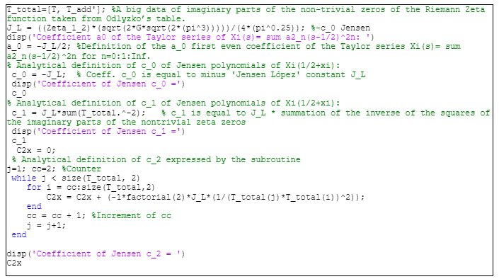
Figure 1: Routine in Matlab for computing the first three coefficients of Jensen polynomials with shift $N=0,c_{0},c_{1}$ and $c_{2}$.

Therefore, the expected numerical coefficients $c_{0},c_{1}$ and $c_{2}$ in Matlab are

$$c_{0}=\frac{-\Gamma\left(\frac{1}{4}\right)\zeta\left(\frac{1}{2}\right)}{4\pi^{\frac{1}{4}}}\approx 0.9942\ldots$$

$$c_{1}=\frac{\Gamma\left(\frac{1}{4}\right)\zeta\left(\frac{1}{2}\right)}{4\pi^{\frac{1}{4}}}\left(\sum_{r=1}^{\infty}\frac{1}{t_{r}^{2}}\right)\approx-0.02297\ldots,$$

$$c_{2}=-\left.\frac{(2!)\Gamma\left(\frac{1}{4}\right)\zeta\left(\frac{1}{2}\right)}{4\pi^{\frac{1}{4}}}\left(\sum_{j=1}^{\infty}\sum_{i=1}^{\infty}\frac{1}{t_{j}{}^{2}t_{i}{}^{2}}\right)\right|_{t_{j}\neq t_{i}}\approx 0.00049172\ldots$$

As a very interesting finding, it has been introduced a remarkable analytical representation for computing some first Jensen’s $c_{n}$, because from Eq.(34) it is possible to infer that, for $n=1$,

$$c_{1}=\frac{\Gamma\left(\frac{1}{4}\right)\zeta\left(\frac{1}{2}\right)}{4\pi^{\frac{1}{4}}}\left(\sum_{r=1}^{\infty}\frac{1}{t_{r}^{2}}\right)=-\left.\frac{d^{2}}{d^{2}x}\xi\left(\frac{1}{2}+ix\right)\right|_{x=0}\approx-0.02297\ldots$$

which means that the second derivative of the Riemann Xi-function evaluated at $\frac{1}{2}+i(0)$ is based on the summation of the inverse of the squares of the imaginary parts of the non-trivial zeros of the Riemann zeta function as seen in Eq.(70). As a result, several values for the even derivatives of $\xi$ will be calculated using the Turán moments, which can be compared to the approximations of Coffey[16].

Taking into consideration that Coffey[16] calculated the even derivatives of the Riemann Xi function at the particular point $s=\left.\left(\frac{1}{2}+ix\right)\right|_{x=0}$, the new results presented in the current article are part of a further computation of some known even derivatives and also new ones as seen in the Table 2 until the last even derivative of order 40 or $\left.\frac{d^{40}}{d^{40}x}\xi\left(\frac{1}{2}+ix\right)\right|_{x=0}$ which is rare or too difficult to be found in the references about the Riemann Xi function, hence it is why this work is novel.

n	$\left.\frac{d^{2n}}{d^{2n}x}\xi\left(\frac{1}{2}+ix\right)\right|_{x=0}$ by $\widehat{\boldsymbol{b}}_{\mathbf{n}}$	$\left.\frac{d^{2n}}{d^{2n}x}\xi\left(\frac{1}{2}+ix\right)\right|_{x=0}$ by $\boldsymbol{c}_{\mathbf{n}}$	$\left.\frac{d^{2n}}{d^{2n}x}\xi\left(\frac{1}{2}+ix\right)\right|_{x=0}$ by $\boldsymbol{{a}_{2\mathbf{n}}}$
0	0.497120778188	0.497120778188	0.497120778188
1	0.0229719443152	0.0229719443152	0.0229719443152
2	0.002962848433688	0.0029628484337	0.0029628484337
3	0.0005992959465976	0.000599295946598	0.000599295946599
4	0.00016096657455	0.000160966574551	0.00016096657455
5	0.0000530386342783	0.0000530386342783	0.0000530386342783
6	0.0000204751152107	0.0000204751152108	0.0000204751152107
7	0.00000898775589325	0.00000898775589327	0.00000898775589325
8	0.00000439330425091	0.0000043933042509	0.00000439330425091
9	0.00000235488338359	0.00000235488338359	0.00000235488338359
10	0.00000136798615159	0.00000136798615159	0.00000136798615159
11	0.000000853314391166	0.000000853314391166	0.000000853314391166
12	0.00000056729724758	0.00000056729724758	0.00000056729724758
13	0.0000003995048218196	0.000000399504821818	0.000000399504821818
14	0.000000296494568267	0.000000296494568267	0.000000296494568267
15	0.0000002308919955117	0.000000230891995511	0.000000230891995511
16	0.0000001879671610623	0.000000187967161062	0.000000187967161062
17	0.0000001594543628979	0.000000159454362897	0.000000159454362897
18	0.0000001405559916949	0.000000140555991695	0.000000140555991694
19	0.0000001284233905038	0.000000128423390504	0.000000128423390503
20	0.0000001213573092303	0.000000121357309231	0.000000121357309231

Table 2: The first twenty-one approximations of the even derivatives of $\xi\left(\frac{1}{2}+ix\right)$ at $\left.\right|_{x=0}$.

The first twenty-one even derivatives of $\xi\left(\frac{1}{2}+ix\right)$ at $\left.\right|_{x=0}$ calculated on Matlab by using the $\widehat{b}_{\mathbf{n}},c_{\mathbf{n}}$ and $a_{2\mathbf{n}}$. Here can be appreciated that the three columns contain practically the same results since they are equivalent ways to compute the values. The precision will depend on the decimal places of the coefficients used.

When inspecting $\mathrm{Eq}(34)$, it is rewritten in terms of $a_{2n}$ as follows

$$\left.\frac{d^{2n}}{d^{2n}x}\xi\left(\frac{1}{2}+ix\right)\right|_{x=0}=(2n)!(-1)^{2n}a_{2n}=(2n)!a_{2n},$$

or also by its equivalent version based on the coefficients of the Jensen polynomials $c_{n}$

$$\left.\frac{d^{2n}}{d^{2n}x}\xi\left(\frac{1}{2}+ix\right)\right|_{x=0}=(-1)^{n}\frac{(2n)!}{2(n!)}c_{n},$$

and a third way based on the Turán moments corresponding to the analysis of the Eq.(38) and Eq.(39), which lets conclude that

$$\left.\frac{d^{2n}}{d^{2n}x}\xi\left(\frac{1}{2}+ix\right)\right|_{x=0}=(2n)!a_{2n}=(2n)!\frac{8.\left(2^{2n}\right)\widehat{b}_{n}}{(2n)!}=8\left(2^{2n}\right)\widehat{b}_{n}.$$

By using any of these three representations and the data of the Table 1, it can be calculated any even derivative of $\xi\left(\frac{1}{2}+ix\right)$ at $\left.\right|_{x=0}$ as seen in the Table 2. Moreover, the consistent approximations of such derivatives would prove that the three kind of coefficients are all valid, otherwise they would yield to wrong approximations in the three cases. The Table 2 illustrates the even derivatives from $\left.\frac{d^{(0)}}{d^{(0)}x}\xi\left(\frac{1}{2}+ix\right)\right|_{x=0}$ to $\left.\frac{d^{(40)}}{d^{(40)}x}\xi\left(\frac{1}{2}+ix\right)\right|_{x=0}$, as a result, the researchers can validate the first known even derivatives computed by Coffey [16] that can be found on the page 529 of the journal where the publication was presented, i.e., $\left.\frac{d^{(2)}}{d^{(2)}x}\xi\left(\frac{1}{2}+ix\right)\right|_{x=0}\cong 0.0229719443$, $\left.\frac{d^{(4)}}{d^{(4)}x}\xi\left(\frac{1}{2}+ix\right)\right|_{x=0}\cong 0.0029628484$ and $\left.\frac{d^{(6)}}{d^{(6)}x}\xi\left(\frac{1}{2}+ix\right)\right|_{x=0}\cong 0.0005992959$. Moreover, the even derivatives are all positive accordingly to the results of Coffey.

The m-file for computing the even derivatives can be requested directly from the author as free code, the name is ’Even derivatives.m’, however, it is very easy just to test by a calculator the coefficients of the Table 1 and the equations Eq.(71), Eq.(72) and Eq.(73) in order to generate the data of the Table 2.

Now, the final part of this section shows a formula for the Riemann Xi and Riemann zeta function based on the three types of coefficients discussed before as follow

$$\xi(s)=\sum_{n=0}^{\infty}a_{2n}\left(s-\frac{1}{2}\right)^{2n}\equiv\sum_{n=0}^{\infty}(-1)^{n}\frac{c_{n}}{2(n!)}\left(s-\frac{1}{2}\right)^{2n}\equiv\sum_{n=0}^{\infty}\frac{8.\left(2^{2n}\right)\widehat{b_{n}}}{(2n)!}\left(s-\frac{1}{2}\right)^{2n},$$

and using one the multiples definitions of the Riemann zeta function [17] by the Riemann Xi as

$$\zeta(s)=\xi(s)\frac{\pi^{\frac{s}{2}}}{(s-1)\Gamma\left(1+\frac{s}{2}\right)}=\frac{\pi^{\frac{s}{2}}}{(s-1)\Gamma\left(1+\frac{s}{2}\right)}\sum_{n=0}^{\infty}a_{2n}\left(s-\frac{1}{2}\right)^{2n},$$

and hence, the other two representations based on the coefficients of the Jensen polynomials and the Turán moments thanks to the equivalences inferred before

$$\zeta(s)=\xi(s)\frac{\pi^{\frac{s}{2}}}{(s-1)\Gamma\left(1+\frac{s}{2}\right)}=\frac{\pi^{\frac{s}{2}}}{(s-1)\Gamma\left(1+\frac{s}{2}\right)}\sum_{n=0}^{\infty}(-1)^{n}\frac{c_{n}}{2(n!)}\left(s-\frac{1}{2}\right)^{2n},$$

$$\zeta(s)=\xi(s)\frac{\pi^{\frac{s}{2}}}{(s-1)\Gamma\left(1+\frac{s}{2}\right)}=\frac{\pi^{\frac{s}{2}}}{(s-1)\Gamma\left(1+\frac{s}{2}\right)}\sum_{n=0}^{\infty}\frac{8.\left(2^{2n}\right)\widehat{b}_{n}}{(2n)!}\left(s-\frac{1}{2}\right)^{2n},$$

because the Eq.(37), Eq.(38) and Eq.(39) let define such equivalences. Moreover, the expressions given by Eq.(15) and the successive ones after it that have been studied previously like Eq.(25) and Eq.(26) let formulate a new polynomial series not seen before and whose coefficients would be precisely the $G_{0},G_{1},G_{2},\ldots G_{j},\ldots$ being $G_{0}$ and $G_{1}$ the first well-known coefficients revised previously

$$\frac{1}{2}=G_{0}=\left(\frac{a_{0}}{2^{0}}+\frac{a_{2}}{2^{2}}+\frac{a_{4}}{2^{4}}+\frac{a_{6}}{2^{6}}+\cdots\right)=\sum_{n=0}^{\infty}\frac{a_{2n}}{2^{2n}},$$

$$G_{1}=-\frac{1}{2}\sum_{\rho}\frac{1}{\rho}=\sum_{r=1}^{\infty}\frac{\sigma_{r}}{s_{r}\bar{s}_{r}}=-\sum_{n=1}^{\infty}\frac{4na_{2n}}{2^{2n}}=-\frac{1}{2}\left(1+\frac{\gamma}{2}-\frac{\log(4\pi)}{2}\right)$$

As a result, the partial definition of the Riemann Xi and zeta functions are

$$\xi(s)=\sum_{n=0}^{\infty}a_{2n}\left(s-\frac{1}{2}\right)^{2n}\equiv\frac{1}{2}-\frac{1}{2}\left(1+\frac{\gamma}{2}-\frac{\log(4\pi)}{2}\right)s+G_{2}s^{2}+G_{3}s^{3}+\cdots G_{j}s^{j}+\cdots.$$

$$\zeta(s)=\frac{\pi^{\frac{s}{2}}}{(s-1)\Gamma\left(1+\frac{s}{2}\right)}\left[\frac{1}{2}-\frac{1}{2}\left(1+\frac{\gamma}{2}-\frac{\log(4\pi)}{2}\right)s+G_{2}s^{2}+G_{3}s^{3}+\cdots G_{j}s^{j}+\cdots\right],$$

which are alternative representations when expanding the term $a_{2n}\left(s-\frac{1}{2}\right)^{2n}$ by the binomial theorem applied on $\left(s-\frac{1}{2}\right)^{2n}$. Finally, a graphical representation of the modulus of the Riemann Xi function in Matlab and also the real and imaginary parts of it are presented in the Fig.2 for a small region specified for $0<\operatorname{Real}(s)<1$ and $-15<\operatorname{Imag}(s)<15$, in order to show only the region where the first conjugated non-trivial zeros $s=\frac{1}{2}+i14,1347\ldots$ and $s=\frac{1}{2}-i14,1347\ldots$ are. The modulus has been computed within the rectangle of the complex domain considered by using the analytical expression Eq. (74) based on the Taylor even coefficients $a_{2n}$ which were calculated on the Table 1. As a result, it is a valid approximation for the Riemann Xi function by using those 21 coefficients. It would prove that the coefficients are suitable for a representation of the Riemann Xi function. The algorithm in Matlab generates graphics that can be compared to the same figures that Wolfram [18] has available for the public, as a result, the algorithm launches the same modulus, real and imaginary parts exactly as expected on the domain considered. The Fig. 3 can be checked via Wolfram on the link https://mathworld.wolfram.com/Xi-Function.html and compared to the m.file named ’Riemann Xi modulus.m’. Moreover, typical values like $\zeta\left(\frac{1}{2}\right)\cong 0.497120778188$ and $\zeta(0)=\zeta(1)=0.5$ are computed by the $m$-file through the Taylor series given by Eq. (74).

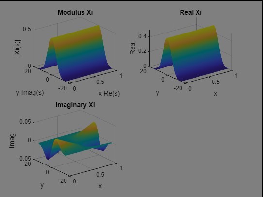
Figure 2: The real and imaginary parts and modulus of the Riemann Xi function represented in Matlab by using the twenty-one $a_{2n}$ ’s.

The m-file leads to represent consistently the expected figures in small intervals, and the first non-trivial zero has been computed approximately $\xi\left(\frac{1}{2}+i14,13\ldots\right)\cong$

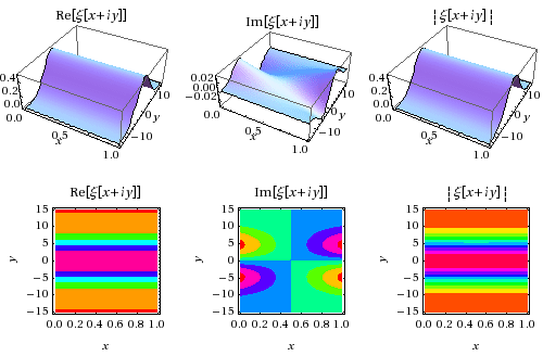
Figure 3: The real and imaginary parts of the Riemann Xi function and its modulus computed by Wolfram. The results are similar to Fig.2

The complete m-file for generating the graphics in Fig.2(can be requested for use from authors as well).

Crucial results that can help to validate the computed even coefficients $a_{2n}$ and $c_{2n}$ and their numerical consequences based on the formulas applied to the data of the Turán moments $\widehat{b_{n}}$ are the Bernoulli numbers [19] based on the Eq.(75) because the fact of using the famous expression for $\zeta(2r)$[20] when the Riemann zeta function is evaluated per every $s=2r$, for $r=0,1,2,3\ldots$, as follows

$$\zeta(2r)=(-1)^{r-1}\frac{(2\pi)^{2r}B_{2r}}{2(2r)!}=\frac{\pi^{r}}{(2r-1)\Gamma(1+r)}\sum_{n=0}^{\infty}a_{2n}\left(2r-\frac{1}{2}\right)^{2n},$$

where $\Gamma(1+r)=r!$ is a well-known property of the Gamma function and $B_{2r}$ are the Bernoulli numbers with even index $2r$. Then, every Bernoulli $B_{2r}$ is written in function of convergent summations based only on the Taylor coefficients $a_{2n}$ as follows

$$B_{2r}=\frac{2(-1)^{r-1}\cdot(2r)!{\pi}^{r}}{(2\pi)^{2r}(2r-1)\mathrm{r}!}\sum_{n=0}^{\infty}a_{2n}\left(2r-\frac{1}{2}\right)^{2n}=\frac{(-1)^{r-1}\cdot(2r)!(2)^{1-2r}}{\pi^{r}(2r-1)\mathrm{r}!}\sum_{n=0}^{\infty}a_{2n}\left(2r-\frac{1}{2}\right)^{2n},$$

which can be evaluated easily by any calculator or software online like Matlab for any specific integer $r=0,1,2,3,\ldots$, for example, when computing the first four even indexes for those Bernoulli numbers based on the known data of the Table 1 , for twenty-one $a_{2n}$ as follows

$$B_{0}=2\sum_{n=0}^{\infty}a_{2n}\left(\frac{1}{2}\right)^{2n}=2\sum_{n=0}^{\infty}\frac{a_{2n}}{4^{n}}\approx 2\left(\frac{a_{0}}{4^{0}}+\frac{a_{2}}{4^{1}}+\cdots+\frac{a_{40}}{4^{20}}\right)\approx 0.4971207781+\frac{\frac{1.14859721576}{100}}{4}+\cdots,$$

$B_{0}\approx 0.999999999999\approx 1$ as expected. Now, for the next Bernoulli numbers with even index

$$B_{2}=\frac{1}{\pi^{1}}\sum_{n=0}^{\infty}a_{2n}\left(\frac{3}{2}\right)^{2n}\approx\frac{1}{\pi}\left[a_{0}+a_{2}\left(\frac{3}{2}\right)^{2}+\cdots+a_{40}\left(\frac{3}{2}\right)^{40}\right]\approx 0.16666666666658\approx\frac{1}{6},$$ (85)

$$B_{4}=\frac{-1}{2\pi^{2}}\sum_{n=0}^{\infty}a_{2n}\left(\frac{7}{2}\right)^{2n}\approx\frac{-1}{2\pi^{2}}\left[a_{0}+a_{2}\left(\frac{7}{2}\right)^{2}+\cdots+a_{40}\left(\frac{7}{2}\right)^{40}\right]\approx-0.03333\ldots\approx-\frac{1}{30},$$ (86)

$$B_{6}=\frac{3}{4\pi^{3}}\sum_{n=0}^{\infty}a_{2n}\left(\frac{11}{2}\right)^{2n}\approx\frac{3}{4\pi^{3}}\left[a_{0}+a_{2}\left(\frac{11}{2}\right)^{2}+\cdots+a_{40}\left(\frac{11}{2}\right)^{40}\right]\approx 0.0238\ldots\approx\frac{1}{42}.$$ (87)

Anyone who tests more Bernoulli numbers $B_{2r}$ with the help of Eq.(83) will prove consistently that such numbers are inferred in this way. The results for the Eq.(41) and the Eq.(46) are undoubtedly related to those findings. Until now, nobody had discovered that the Bernoulli numbers could have an evident connection with the Turán moments and the coefficients of Jensen polynomials as seen before, which has been numerically derived by the computation and, above all, the proper analysis of such numbers. As a result, Eq.(83) can be written in two ways as well, one for the Turán moments, Eq.(88), and a second one, Eq.(89), over the coefficients of Jensen polynomials, being the Eq.(89) deeply related to the fact of considering the entire function $\xi$ evaluated as $\xi\left(\frac{1}{2}+ix\right)$ when the scenario of hyperbolicity of the Jensen polynomials is accepted according to the recent works of researchers like Griffin et al. [21], who have proved many significant cases for such property on the Jensen polynomials which in the current article would be extremely difficult to be contradicted against the variety of formulas obtained and presented here considering the real part of the non-trivial zeros of the Riemann zeta function lying strictly on the critical line. From this scenario, the Bernoulli numbers $B_{2r}$ have an important connection with the Turán moments and coefficients of Jensen polynomials as follows

$$B_{2r}=\frac{16(-1)^{r-1}\cdot(2r)!2^{-2r}}{(\pi)^{r}(2r-1)\mathrm{r}!}\sum_{n=0}^{\infty}\frac{2^{2n}\widehat{b_{\mathrm{n}}}\left(2r-\frac{1}{2}\right)^{2n}}{(2n)!}$$

$$B_{2r}=\frac{(-1)^{r-1}\cdot(2r)!2^{1-2r}}{(\pi)^{r}(2r-1)\mathrm{r}!}\sum_{n=0}^{\infty}\frac{(-1)^{n}c_{n}\left(2r-\frac{1}{2}\right)^{2n}}{2(n)!},$$

Remembering also that with the help of the known expression that links the Gregory coefficients $G_{n}$ of order 1 introduced in the beginning of this article

$$G_{n}=-\frac{B_{n}{}^{(n-1)}}{(n-1)\cdot(n!)}$$

we were able to find that every $G_{2r}=G_{2r}(1)$, with $r=1,2,3$ and the respective $c_{n}$ and $\widehat{b_{n}}$ can be linked as

$$B_{2r}=\frac{16(-1)^{r-1}\cdot(2r)!2^{-2r}}{(\pi)^{r}(2r-1)\mathrm{r}!}\sum\limits_{n=0}^{\infty}\frac{2^{2n}\widehat{b_{n}}\left(2r-\frac{1}{2}\right)^{2n}}{(2n)!}=\sqrt[2r-1]{-G_{2r}(2r-1)\cdot(2r)!}$$

$$B_{2r}=\frac{(-1)^{r-1}\cdot(2r)!2^{1-2r}}{(\pi)^{r}(2r-1)r!}\sum\limits_{n=0}^{\infty}\frac{(-1)^{n}c_{n}\left(2r-\frac{1}{2}\right)^{2n}}{2(n)!}=\sqrt[2r-1]{-G_{2r}(2r-1)\cdot(2r)!}$$

where each $B_{0},B_{2},B_{4}\ldots$ can be deduced by a similar way computed by Eq.(83), since Eq.(83) can be modified by the equivalences studied before $C_{n}=2(n!)(-1)^{n}a_{2n}=\frac{16(-1)^{n}(n!)2^{2n}}{(2n)!}\widehat{b_{n}}$ in Eq.(38) and Eq.(39) which lead to write such expressions, only possible if the entire function $\xi$ evaluated in the complex values like $\frac{1}{2}+ix$ is agreed to the phenomen of hyperbolicity of the Jensen polynomials or the validity of the Riemann hypothesis. The formulation of the Bernoulli numbers for even indexes, the calculation of the even derivatives of the Riemann Xi function at the special point $\frac{1}{2}+i(0)$ and the novel three representation formulas for the Euler-Mascheroni constant would be very important consequences for supporting the validity of the Riemann hypothesis, which is presented in this article for pointing out the extreme difficulties to try to adjust the entire function in other ways that violated the Riemann hypothesis itself. The Hadamard product and the Taylor series for $\xi\left(\frac{1}{2}+ix\right)$ would be hardly feasible against the evidence provided on the data of the Table 1 and Table 2 and the formulations derived from these. As a result, the Eq.(46), $\gamma=\log(4\pi)-2+$ $\left(2^{7}\right)\sum\limits_{n=1}^{\infty}\frac{n\widehat{b_{n}}}{(2n)!}$, is consistent with the formula for the summation over the Bernoulli numbers[22], in Eq.(90), that computes the approximation for the Euler-Mascheroni constant as follows

$$\gamma=\frac{1}{2}+\sum_{n=1}^{\infty}\frac{B_{2n}}{(2n)}$$

the unexpected connection between the Euler-Mascheroni constant and the Turán moments is not a surprise if it is noticed that there is already a well-known formula, Eq.(90), that lets consider an expansion on the Bernoulli numbers. Of course, other infinite sets of relevant numbers like the Gregory coefficients [23] and the Cauchy numbers of the second kind [24] can describe special summations on those ones which converge to the Euler-Mascheroni constant. Now, the evidence shows that three new sets of coefficients $a_{2n},\widehat{b_{n}}$ and $C_{n}$, can contribute to represent this important constant as it has been inferred in the current article. Moreover, the equivalences on both sides of Eq.(46) and Eq.(90) lead to get this possible formulation

$$\gamma=\frac{1}{2}+\sum_{n=1}^{\infty}\frac{B_{2n}}{(2n)}=\log(4\pi)-2+\left(2^{7}\right)\sum_{n=1}^{\infty}\frac{n\widehat{b_{n}}}{(2n)!},$$

which exposes that the summation of the Bernoulli numbers in that way has a final effect that is equivalent to introduce the Turán moments and the number $\pi$ in the other special summation. As a result, many sets of numbers produce relevant summations that represent the same constant.

The Turán inequalities and Laguerre inequalities [25] are accomplished as well when the numerical values for the coefficients $C_{n}$ of the Jensen polynomials are examined

$$C_{n}{}^{2}-C_{n-1}C_{n+1}>0,\quad n\geq 1,$$

for example,

$$C_{1}^{2}-C_{0}C_{2}>0,$$

because, when testing $C_{0}=0.994241556376,C_{1}=-2.29719443152\left(10^{-2}\right)$ and $C_{2}=$ $4.93808072283\left(10^{-4}\right)$

$$\left(-2.29719443152\left(10^{-2}\right)\right)^{2}-0.994241556376\left(4.93808072283\left(10^{-4}\right)\right)\approx 3.674\left(10^{-5}\right)>0$$

and for the consecutive values $C_{1},C_{2},C_{3}$

$$C_{2}{}^{2}-C_{1}C_{3}>0,$$

$$\left(4.93808072283\left(10^{-4}\right)\right)^{2}-\left(-2.29719443152\left(10^{-2}\right)\right)\left(-9.98826577664\left(10^{-6}\right)\right)\approx 1.4396\left(10^{-8}\right)>0$$

Such inequalities must be accomplished strictly for all the successive coefficients considered, which is valid here because these are the correct coefficients of the Jensen polynomials.


Discussion

The numerical results presented in this article are evidently good approximations for the coefficients of the Jensen polynomials and the even Taylor coefficients for the Riemann Xi function which have been inferred from a solid basis like the Csordas, Norfolk and Varga’s work mentioned before in the references. The formulation of these coefficients have let discover an interesting formula for the Euler-Mascheroni constant which is a novel representation. The results, numerically said, are a clear proof of the consistency of these numbers, being the main proof, the possibility to represent various values of the Riemann Xi function and, above all, its graphics, i.e., its modulus, real and imaginary parts. The references in mathematics regarding the Turán moments and their immediate connection with the coefficients of the Jensen polynomials, Bernoulli numbers and the hyperbolicity of the Jensen polynomials are just a little part of a reduced group of publications when discussing the structure of the Riemann Xi function, and hence, the Riemann zeta function, which is really a pity because not many researchers have considered the potential of the analysis of interesting sets of Taylor coefficients as seen in this article and other equivalent numbers that could help to understand the field of number theory in a better way. Regarding the possible future directions of this research, the newest ideas are based on the similitude or parallelism between these two expressions, Eq.(97) for the formulation already seen

$$\frac{\zeta(s)(s-1)\Gamma\left(1+\frac{s}{2}\right)}{8\pi^{\frac{s}{2}}}-\widehat{b_{0}}=\sum_{n=1}^{\infty}\frac{2^{2n}\widehat{b_{n}}\left(s-\frac{1}{2}\right)^{2n}}{(2n)!},$$

and the definition of the series form for the hyperbolic cotangent function [26] which involves the Bernoulli numbers as follows

$$\left(s-\frac{1}{2}\right)\operatorname{coth}\left(s-\frac{1}{2}\right)-B_{0}=\sum_{n=1}^{\infty}\frac{2^{2n}B_{2n}\left(s-\frac{1}{2}\right)^{2n}}{(2n)!}.$$

From these two equations is thought to involve the Bernoulli numbers within the representation of a compact formula, still being developed in multiple hypothesis, due to the tremendous parallelism that these two series present within this context. The only difference between Eq.(97) and Eq.(98) is the use of either the Turán moments $\widehat{b_{n}}$ or the $B_{2n}$ which would lead to describe the possible connection between the Riemann zeta function $\zeta(s)$ and other special functions like the hyperbolic trigonometric functions. This idea is majestic because there exist a possible link to the Riesz function [27] and the suggestions of using Eq.(97) and Eq.(98), since the Riesz function has this interesting definition

$$R(x)=2\sum_{n=1}^{\infty}\frac{n^{\bar{n}}x^{n}}{(2\pi)^{2n}\left(\frac{B_{2n}}{2n}\right)},$$

being $n^{\bar{n}}$ the rising factorial power.

The essence of this function is appreciated when considering $F(x)=\frac{1}{2}\operatorname{Riesz}\left(4\pi^{2}x\right)$ since its Laurent series is related precisely to the concept of hyperbolic cotangent function as seen in this expression

$$\left(\frac{x}{2}\right)\operatorname{coth}\left(\frac{x}{2}\right)=\sum_{n=0}^{\infty}C_{n}x^{n}=1+\frac{1}{12}x^{2}-\frac{1}{720}x^{4}+\cdots,$$

which lets define the series form for

$$F(x)=\frac{1}{2}\operatorname{Ries}z\left(4\pi^{2}x\right)=\sum_{n=1}^{\infty}\frac{x^{n}}{c_{2n}(n-1)!}=12x-720x^{2}+15120x^{3}\ldots,$$

that is also written in the references as

$$F(x)=\sum_{n=1}^{\infty}\frac{n^{\overline{n+1}}x^{n}}{B_{2n}},$$

the perspective of this work is to develop a model that lets write the Turán moments, coefficients of the Jensen polynomials and even Taylor coefficients strictly in function of the Bernoulli numbers or others like the Gregory coefficients of higher order, which would be a tremendous finding in mathematics because would let write the Riemann zeta function and Riemann Xi strictly in function of the Gregory coefficients of higher orders. The initial speculations based on the hyperbolic trigonometric functions, particularly about the hyperbolic cotangent, seem to point out that at least in some complex points the hyperbolic cotangent is candidate to be used within a model for the Riemann $\mathrm{Xi}$ and zeta functions.

A forced equivalence that is still under revision for future development is the idea of equating the Eq.(97) and Eq.(98) for representing some domains of the Riemann zeta function, in fact, the partial model of a compact analytical definition is highly based in transcendental functions that nobody had suspected before, a slight set of parameters, about a novel model known as the hypothetical parameters, for example, $a$ and $b$, could help to equate the expressions and cover all the complex domains considered conveniently by

$$\frac{\zeta(s)(s-1)\Gamma\left(1+\frac{s}{2}\right)}{{8\pi^{\frac{s}{2}}}}-\widehat{b_{0}}=\left((\mathbf{a})\cdot\mathbf{s}-\frac{b}{2}\right)\operatorname{coth}\left((\mathbf{a})\cdot\mathbf{s}-\frac{b}{2}\right)-B_{0}=\sum_{n=1}^{\infty}\frac{2^{2n}B_{2n}\left((a)\cdot s-\frac{b}{2}\right)^{2n}}{(2n)!},$$

the analysis of that kind of expressions, of course, improved by meticulous theorems, could be the key for resolving the mystery of writing a final version for the Riemann Xi and zeta function. Some tests have shown that using transcendental equations could help to find these parameters and define the way of the Riemann zeta function and Xi as well. This is the future part of this research.


Conclusions

The most important conclusion regarding the coefficients of the Taylor series for the Riemann Xi function is the surprising consequence that the convergence of the special summations involving the non-trivial zeros of $\zeta$ seems to define exactly the coefficients of the Jensen polynomials which are useful for supporting the idea of the hyperbolicity of this kind of polynomials regarding the work of Griffin, Ono and other authors. If the current research shows that after computing the first coefficients of Jensen polynomials by the assumption of the real part of the non-trivial zeros of the Riemann zeta function like $\frac{1}{2}$, then the structure of the Hadamard product of the Riemann Xi function is clearly exact to the expansion for the Taylor series of the Riemann Xi function around $s_{0}=\frac{1}{2}+i\cdot t_{0}$, being $t_{0}$ the imaginary part of any non-trivial zero of the Riemann zeta function.

The never told before comparison between the Hadamard product and the Taylor series of the Riemann Xi function is an important equivalence that according to this article would lead to deduce veridic consequences when ${s}_{{0}}=\frac{1}{2}+{i}\cdot{t}_{{0}}$, because the formulas depend on this approach, as a result, how the Euler-Mascheroni constant, Bernoulli numbers, even derivatives of the Riemann Xi function and other relationships discovered could be written with such exactness and based on solid true experimental results if the Riemann hypothesis had been false? That is the most important conclusion that the readers of this article should take into consideration after examining the complete work presented here.

References

[1] L. Euler, De summatione innumerabilium progressionum, Comment. Acad. Sci. Petrop. 5 (1738), 91–105. (presented March 5, 1731) (Opera Omnia, Series 1, Vol. 14, pp. 25–41). [E20] [2.2, 2.4]
[2] H.M. Edwards. The Function . §1.8 in Riemann’s Zeta Function. New York: Dover, pp. 16-18, 2001.
[4] M. DeFranco. “On properties of the Taylor series coefficients of the Riemann xi function at s=1/2”. (2019). [Online]. Available: https://arxiv.org/abs/1907.08984
[5] G. Csordas, T.S. Norfolk, R.S. Varga. The Riemann Hypothesis and the Turán Inequalities. [Online]. Available: https://doi.org/10.2307/2000378
[6] J.B. Keiper. (1992). ”Power series expansions of Riemann’s xi function”. Mathematics of Computation. 58 (198): 765–773. Bibcode:1992MaCom..58..765K. doi:10.1090/S0025-5718-1992-1122072-5.
[7] F. Alhargan. A Concise Proof of the Riemann Hypothesis Based on Hadamard Product. 2021. ffhal-01819208v4.
[8] M. Griffin et al., “Jensen polynomials for the Riemann zeta function and other sequences”. (2019). [Online]. Available: https://doi.org/10.1073/pnas.1902572116.
[9] Enrico Bombieri. “New progress on the zeta function: From old conjectures to a major breakthrough”. (2019). [Online]. Available: https://www.pnas.org/content/116/23/11085.
[16] Relations and positivity results for the derivatives of the Riemann function. Journal of Computational and Applied Mathematics. Volume 166, Issue 2, 15 April 2004, Pages 525-534. [Online]. Available: https://www.sciencedirect.com/science/article/pii/S0377042703007970
[24] G. Csordas. Turán-type inequalities and the distribution of zeros of entire functions. From the book Number Theory, Analysis, and Combinatorics. [Online]. Available: https://doi.org/10.1515/9783110282429.25 (accessed on 1 of January 2021).
[26] Herbert S. Wilf. “On the zeros of Riesz’ function in the analytic theory of numbers”. [Online]. Available: Illinois J. Math. 8(4): 639-641 (December 1964). DOI: 10.1215/ijm/1256059463 (accessed on the 1 of September of 2021).