Value Activation for Bias Alleviation: Generalized-activated Deep Double Deterministic Policy Gradients

Abstract

It is vital to accurately estimate the value function in Deep Reinforcement Learning (DRL) such that the agent could execute proper actions instead of suboptimal ones. However, existing actor-critic methods suffer more or less from underestimation bias or overestimation bias, which negatively affect their performance. In this paper, we reveal a simple but effective principle: proper value correction benefits bias alleviation, where we propose the generalized-activated weighting operator that uses any non-decreasing function, namely activation function, as weights for better value estimation. Particularly, we integrate the generalized-activated weighting operator into value estimation and introduce a novel algorithm, Generalized-activated Deep Double Deterministic Policy Gradients (GD3). We theoretically show that GD3 is capable of alleviating the potential estimation bias. We interestingly find that simple activation functions lead to satisfying performance with no additional tricks, and could contribute to faster convergence. Experimental results on numerous challenging continuous control tasks show that GD3 with task-specific activation outperforms the common baseline methods. We also uncover a fact that fine-tuning the polynomial activation function achieves superior results on most of the tasks. Codes will be available upon publication.

We propose a novel generalized-activated weighting operator for bias alleviation in deep reinforcement learning.

We theoretically and experimentally show that the distance between the max operator and the generalized-activated weighting operator can be bounded.

We show theoretically and experimentally that generalized-activated weighting operator helps alleviate both underestimation bias and overestimation bias.

We find that simple activation functions are enough for amazing performance without any tricks and special design for activation function.

1 Introduction

Reinforcement Learning (RL) has achieved remarkable progress in continuous control scenarios in recent years (Mnih et al. (2015)). Actor-critic methods (Konda and Tsitsiklis (2000)) are widely adopted in continuous control problems, which relies on the critic to estimate the value function under the current state and execute policy via an actor. In actor-critic-style methods, it is important for the critic to estimate the value function in a good manner such that the actor can be driven to learn better policy. However, existing methods are far from satisfying.

As an extension of Deterministic Policy Gradient (DPG) (Silver et al. (2014)), Deep Deterministic Policy Gradient (DDPG) (Lillicrap et al. (2015)) is one of the earliest and most widely-used algorithms. DDPG is designed to operate on a continuous regime with a deterministic policy based on the Actor-Critic method. Although DDPG performs well in many continuous control tasks, it actually suffers from overestimation bias (Fujimoto et al. (2018)), as is often reported in Deep Q-Network (DQN) (van Hasselt et al. (2016); Zhang et al. (2017)). Such phenomenon is caused by the fact that the actor network in DDPG learns to take action according to the maximal value estimated by the critic network, which would result in poor performance. To address the function approximation error in DDPG, Fujimoto et al. propose Twin Delayed Deep Deterministic Policy Gradient (TD3) algorithm (Fujimoto et al. (2018)) by training two critic networks and updating with the smaller estimated value to tackle the problem, which is inspired to the idea of Double DQN (van Hasselt et al. (2016)). TD3 significantly outperforms DDPG with reduced overestimation bias with Clipped Double Q-learning and delayed update of target networks. While it turns out that TD3 may induce large underestimation bias (Ciosek et al. (2019)).

In this paper, we reveal a simple but effective principle: proper value correction benefits bias alleviation, i.e., the bias in value estimation can be eased. Particularly, we propose a novel and general function transformation framework for value estimation bias alleviation in deep reinforcement learning. Our method leverages any non-decreasing function, namely activation function, and leads to a novel generalized-activated weighting operator. The operator is an activation to the estimated Q values which generates a new distribution with a one-to-one mapping to the original value distribution as shown in Fig 1. The activated distribution reveals the importance of the estimated value in the distribution. Intuitively, we can get a better value estimation by weighting these estimated values. We show that the generalized-activated weighting operator helps alleviate overestimation bias in DDPG if built upon single critic network, where we develop Generalized-activated Deep Deterministic Policy Gradient (GD2) algorithm. It also helps relieve underestimation bias in TD3 if built upon double critics, which incurs Generalized-activated Deep Double Deterministic Policy Gradients (GD3) algorithm. Extensive experimental results on challenging continuous control tasks in OpenAI Gym (Brockman et al. (2016)) show that GD3 significantly outperforms common baseline methods and could achieve better performance and sample efficiency with task-specific activations.

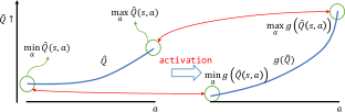
Figure 1: How activation function changes the distribution of value function over action space. Large Q would become larger after being activated.

Our contributions can be summarized as follows:

• We propose a novel generalized-activated weighting operator for bias alleviation in deep reinforcement learning.

• We theoretically and experimentally show that the distance between the max operator and the generalized-activated weighting operator can be bounded.

• We show theoretically and experimentally that generalized-activated weighting operator helps alleviate both underestimation bias and overestimation bias.

• We find that simple activation functions are enough for amazing performance without any tricks and special design for activation function.

The rest of the paper is organized as follows: Section 2 is a collection of related work; Section 3 gives preliminaries of reinforcement learning; Section 4 formally defines generalized-activated weighting operator and gives theoretical analysis; Section 5 develops GD2 and GD3 algorithm; Section 6 presents detailed experimental results of GD3; Section 7 concludes the paper.

2 Related Work

Reinforcement learning has witnessed impressive progress in recent years (Mnih et al. (2015); Silver et al. (2015); Arulkumaran et al. (2019); Mirhoseini et al. (2020)), and has been applied into many fields, like games (Ye et al. (2020a, b); Liu et al. (2021)), complex system control (Chen et al. (2021); Huang et al. (2020); Pálos and Huszák (2020)), financial trading (Ma et al. (2021)), recommendation (Liu et al. (2020); Pei et al. (2019)), etc.

Actor-Critic methods (Konda and Tsitsiklis (2000)) are widely used in reinforcement learning which involve value function approximation for the estimation of policy gradient (Sutton et al. (2000)). Many improvements and advances upon actor-critic methods are proposed in recent years, including asynchronous method (Mnih et al. (2016)), maximum entropy reinforcement learning (Haarnoja et al. (2018)), distributional RL Bellemare et al. (2017); Ma et al. (2020), offline RL (batch RL) Levine et al. (2020); Yang et al. (2021); Jiang and Lu (2021), etc. DDPG (Lillicrap et al. (2015)), which is built upon actor-critic and sheds lights to continuous control, extends DPG (Silver et al. (2014)) algorithm to deep reinforcement learning. There are many works that are built on and improve DDPG, such as model-based (Gu et al. (2016)), distributed (Popov et al. (2017)), distributional (Barth-Maron et al. (2018); Bellemare et al. (2017)), prioritized experience replay (Horgan et al. (2018)) and multi-step returns (Meng et al. (2020)). While DDPG may cause devastating overestimation bias (Fujimoto et al. (2018)) which is also often reported in DQN and is relieved by Double DQN in discrete regime (van Hasselt et al. (2016)).

In this paper, we are interested in ways of getting a better value estimator for continuous control tasks. How to obtain satisfying value estimation remains an important problem to be solved in reinforcement learning, and has been widely studied (Pan et al. (2020); Jiafei et al. (2021); Kuznetsov et al. (2021)). TD3 (Fujimoto et al. (2018)) improves value estimation of DDPG with Clipped Double Q-learning while it can lead to large underestimation bias (Ciosek et al. (2019)). Kuznetsov et al. adopt a truncated ensemble of distributional critics for controlling overestimation in continuous setting (Kuznetsov et al. (2020)). Moskovitz et al. balance between optimism and pessimism with a multi-arm bandit aiming at maximizing the immediate performance improvement (Moskovitz et al. (2021)). Weighted Delayed DDPG (He and Hou (2020)) adopts weighted sum of the minimum of Q-functions and the average of an ensemble of Q-functions for overestimation bias alleviation. A recent work (Cetin and Çeliktutan (2021)) studies a flexible data-driven way of bias controlling method with the aid of epistemic uncertainty. Different from these advances, we focus on improving the value estimation by leveraging any non-decreasing activation functions. Our method does not involve training critic ensembles, estimating uncertainty or bandit components, which makes it much lighter and efficient.

Most relevant to our work is SD3 (Pan et al. (2020)), which uses the softmax operator on value function to get a softer value estimation. It is worth noting that SD3 is a special case of our method, i.e., we set the activation function as exponential and then GD3 would degenerate into SD3. Also, according to our experimental results, exponential activation is often not the optimal activation function (see Section 6). GD3 is a general and effective method for bias alleviation in continuous control.

3 Preliminaries

Reinforcement learning aims to maximize expected discounted cumulative future reward and it can be formulated by a Markov Decision Process (MDP) which is made up of state space $\mathcal{S}$, action space $\mathcal{A}$, reward function $r:\mathcal{S}\times\mathcal{A}\rightarrow\mathbb{R}$, transition probability distribution $p(s^{\prime}|s,a)$, and discount factor $\gamma\in[0,1]$. In this paper, we consider continuous action space and reward function scenarios and assume they are bounded as required in (Pan et al. (2020); Silver et al. (2014)), i.e., $r(s,a)\in[-R_{\mathrm{max}},R_{\mathrm{max}}],\forall s,a$. DDPG is an off-policy algorithm for continuous control which learns deterministic policy $\pi(\cdot;\phi)$ instead of stochastic policy as in Q learning (Watkins and Cornish Hellaby (1989)). It is an extension of Deterministic Policy Gradient (DPG) (Silver et al. (2014)) with deep neural networks and actor-critic structure. Since it is expensive to take max operator on continuous action space directly, the critic of DDPG estimates Q value by maximizing the Q-function $Q$: $\mathcal{S}\times\mathcal{A}\rightarrow\mathbb{R}$ to approximate max operator and is updated by minimizing $\mathbb{E}[(y_{t}-Q(s_{t},a_{t};\theta))^{2}]$, where $y_{t}=r_{t}+\gamma Q(s_{t+1},\pi(s_{t+1}))$. $r_{t}$ is the scalar reward at time step $t$ and $Q(s_{t},a_{t};\theta)$ parameterized by $\theta$ is estimated by neural networks to approximate the true value $\theta^{\mathrm{true}}$; The actor decides what action to take and is updated via deterministic policy gradient:

$$\nabla_{\phi}J(\pi(\cdot;\phi))=\mathbb{E}[\nabla_{\phi}(\pi(s;\phi))\nabla_{a}Q(s,a;\theta)|_{a=\pi(s,\phi)}].$$ (1)

4 Generalized-activated Weighting Operator

4.1 How to better estimate value function?

In Actor-Critic, it is crucial for the critic network to effectively estimate the value function as the performance of the actor network is hugely influenced by its counterpart critic. TD3 alleviates the overestimation bias in DDPG (Fujimoto et al. (2018)) while it may result in large underestimation bias (Ciosek et al. (2019)). Both of the biases would negatively affect the performance of the algorithm. We, however, propose to do value estimate correction using any non-decreasing functions for more balanced value estimation. With function transformation, a new distribution for Q-values can be acquired. We name the transformation from one distribution to another as activation, and the corresponding non-decreasing function as activation function.

Fig 1 shows the process of activation from original value function distribution to activated one via a non-decreasing function $g(\cdot;\bm{\psi})$ parameterized by $\bm{\psi}$ where $\bm{\psi}$ can be a scalar or a vector. Note that we suppose that one action corresponds to one unique value function here for simplicity and better illustration which may not be necessarily true in the continuous regime. We require the activation function to be non-decreasing as we need larger weight upon larger Q value to prevent devastating underestimation bias. The activation process is actually a one-to-one order-preserving mapping (as the red line in Fig 1 shows) from one probability space to another probability space with larger variance, i.e., the diversity of the value distribution would become larger after being activated.

The operator $\mathcal{T}$ is a value estimator which gives estimation of value function given state $s$ and is used to update target value, i.e. $y=r+\gamma\mathcal{T}(s)$. Then we could give a formal definition of the generalized-activated weighting operator.

Definition 1.

Let $g(\cdot;\bm{\psi})$ be a non-decreasing function parameterized by $\bm{\psi}$, then the generalized-activated weighting operator is defined as:

$$GA_{g}(Q(s,\pi(s));\bm{\psi})=\int_{a\in\mathcal{A}}\frac{g(Q(s,a);\bm{\psi})Q(s,a)}{\int_{a^{\prime}\in\mathcal{A}}g(Q(s,a^{\prime});\bm{\psi})da^{\prime}}da.$$ (2)

4.2 Theoretical Analysis

Theorem 1 and Theorem 2 guarantee the rationality and practicability of generalized-activated weighting operator. Note that some proofs of theorems in this part and section 5 are deferred to Appendix A.

We first give a simple lemma under the bounded reward function assumption.

Lemma 1.

The Q value is bounded, i.e., $-\frac{R_{\mathrm{max}}}{1-\gamma}\leq Q(s,a)\leq\frac{R_{\mathrm{max}}}{1-\gamma},\forall s,a$.

Proof.

By definition, we have

$$Q(s,a) =\mathbb{E}_{\pi}\left[\sum_{t=1}^{T}\gamma^{t}r(s_{t},a_{t})\bigg{|}a\sim\pi(\cdot|s)\right]$$

$$\leq\mathbb{E}_{\pi}\left[R_{\mathrm{max}}\sum_{t=1}^{T}\gamma^{t}\right]=\frac{R_{\mathrm{max}}}{1-\gamma}.$$

Similarly, we have

$$Q(s,a) =\mathbb{E}_{\pi}\left[\sum_{t=1}^{T}\gamma^{t}r(s_{t},a_{t})\bigg{|}a\sim\pi(\cdot|s)\right]$$

$$\geq\mathbb{E}_{\pi}\left[-R_{\mathrm{max}}\sum_{t=1}^{T}\gamma^{t}\right]=-\frac{R_{\mathrm{max}}}{1-\gamma}.$$

∎

Our first main result reveals that the distance between generalized-activated weighting operator and the max operator can be bounded.

Theorem 1.

Denote $\mathcal{C}(Q,s,\epsilon)=\{a|a\in\mathcal{A},Q(s,a)\geq\max_{a}Q(s,a)-\epsilon\}$, $F(Q,s,\epsilon)=\int_{a\in\mathcal{C}(Q,s,\epsilon)}1da$ for $\epsilon>0$. Let $\beta\in\mathcal{B}$ such that $g(Q(s,a);\bm{\psi})\geq\exp(\beta Q(s,a))$, and denote $T(Q^{*})$ as the maximum value of the function $T(Q(s,a);\bm{\psi},\beta)=\frac{1}{\beta}\ln g(Q(s,a);\bm{\psi})-Q(s,a)$ for some non-decreasing functions $g(Q(s,a);\bm{\psi})$, then the difference between the max operator and generalized-activated weighting operator is bounded:

$$0\leq\max_{a}Q(s,a)-GA_{g}(Q(s,\pi(s));\bm{\psi})\leq M(Q,\epsilon;\bm{\psi},\beta),$$

where $M(Q,\epsilon;\bm{\psi},\beta)=\epsilon+\frac{\int_{a\in\mathcal{A}}1da-1+\ln F(Q,s,\epsilon)}{\beta}+T(Q^{*})$.

Proof.

See Appendix A.1. ∎

Remark 1: If we adopt exponential function as activation function, then (1) $T(Q^{*})$ would become a constant; (2) the generalized-activated weighting operator would degenerate to softmax operator, which is recently studied in (Pan et al. (2020)).

Remark 2: The upper bound would be 0 if $Q(s,a)$ is a constant function since

$$GA_{g}(Q(s,\pi(s));\psi) =\int_{a\in\mathcal{A}}\frac{g(Q(s,a);\psi)Q(s,a)}{\int_{a^{\prime}\in\mathcal{A}}g(Q(s,a^{\prime});\psi)da^{\prime}}da$$

$$=Q(s,a)=\max_{a}Q(s,a).$$

The upper bound would converge to $\epsilon+T(Q^{*})$ with $\beta\rightarrow\infty$.

$T(Q^{*})$ denotes the cost of the generalization from exponential family to arbitrary non-decreasing functions which measures the maximal distance between an arbitrary non-decreasing function to exponential activation parameterized by $\beta$. If $T(Q^{*})$ always lies in a reasonable region, then the upper bound would be $O(\frac{1}{\beta})$. In fact, the distance between max operator and generalized-activated weighting operator is reasonable enough in practice where detailed discussion in available in section 6.1.

Lemma 2 says that we can always find such non-decreasing functions satisfying the inequality $g(Q(s,a);\bm{\psi})\geq\exp(\beta Q(s,a))$, which ensures the rationality of the theorem.

Lemma 2.

The support set $\mathcal{B}$ containing $\beta$ such that for some non-decreasing functions $g(\cdot;\psi)$, $g(Q;\psi)\geq\exp(\beta Q)$, is non-empty, i.e., $|\mathcal{B}|>$ 0.

Proof.

Note that when $\beta\rightarrow 0$, i.e., $\beta$ is sufficiently small, the exponential operator would become similar to that of linear operator, i.e., $\exp(\beta Q(s,a))\approx 1+\beta Q$ if $|\beta|<\epsilon$. Hence we can always design some non-decreasing functions with parameter $\psi$ such that $g(Q(s,a);\psi)\geq\exp(\beta Q(s,a))$, e.g., $g(Q(s,a);\psi)=1+2Q(s,a)$ as $2\gg\beta$. Furthermore, the $Q$-value is bounded based on Lemma 1, therefore as long as $\beta$ is small enough, we can always find some non-decreasing functions that satisfy the constraint. Hence $|\mathcal{B}|>0$. ∎

After applying generalized-activated weighting operator, the value function would be updated by $Q_{t+1}=r_{t}+\gamma\mathbb{E}_{s^{\prime}\sim p(\cdot|s,a)}[GA_{g}(Q(s,a);\bm{\psi})]$, then by using Theorem 1, the distance of value functions induced by optimal operator and generalized-activate weighting operator is also bounded.

Theorem 2 (Value Iteration).

The distance between the optimal value function $V^{*}$ and the value function weighted by generalized-activated weighting operator is bounded at t-th iteration:

$$\|V_{t}-V^{*}\|_{\infty}\leq\gamma^{t}\|V_{0}(s)-V^{*}(s)\|_{\infty}+N(Q,\epsilon,\gamma;\psi,\beta),$$

where $N(Q,\epsilon,\gamma;\psi,\beta)=\frac{T(Q^{*})}{1-\gamma}+\frac{1}{1-\gamma}\frac{\beta\epsilon+\int_{a\in\mathcal{A}}1da-1}{\beta}-\sum_{k=1}^{t}\gamma^{t-k}\frac{\min_{s}\ln F(Q_{k}(s,\pi(s)),s,\epsilon)}{\beta}$.

Proof.

Note that the optimal value estimation function $V^{*}$ is acquired by the max operator, i.e.,

$$V^{*}(s)=\max_{a\in\mathcal{A}}Q^{*}(s,a).$$ (3)

By definition of generalized-activated weighting operator value iteration, we have

$$|V_{t+1}-V^{*}| =|GA_{g}(Q(s,\pi(s));\psi)-\max_{a}Q^{*}(s,a)|$$

$$\leq|GA_{g}(Q(s,\pi(s));\psi)-\max_{a}Q_{t+1}(s,a)|$$

$$\quad+|\max_{a}Q_{t+1}(s,a)-\max_{a}Q^{*}(s,a)|.$$

By using Theorem 1 and the fact that max operator is non-expansive (Singh et al. (1994)), we have $|\max_{a}Q_{t+1}(s,a)-\max_{a}Q^{*}(s,a)|=\max_{a}|Q_{t+1}(s,a)-Q^{*}(s,a)|\leq\gamma\max_{s^{\prime}}|V_{t}(s^{\prime})-V^{*}(s^{\prime})|$. Then,

$$\|V_{t+1}(s)-V^{*}(s)\|_{\infty} \leq\gamma\|V_{t}(s)-V^{*}(s)\|_{\infty}+\epsilon+T(Q^{*})$$

$$\,+\frac{\int_{a\in\mathcal{A}}1da-1-\min_{s}\ln F(Q_{t+1},s,\epsilon)}{\beta}.$$

Doing iteration, we have

$$\|V_{t}(s)-V^{*}(s)\|_{\infty}$$

$$\leq\gamma^{t}\|V_{0}(s)-V^{*}(s)\|_{\infty}+\sum_{k=1}^{t}\gamma^{t-k}(\epsilon+T(Q^{*}))$$

$$\qquad-\sum_{k=1}^{t}\frac{\min_{s}\ln F(Q_{t+1},s,\epsilon)}{\beta}+\sum_{k=1}^{t}\frac{\int_{a\in\mathcal{A}}1da-1}{\beta}$$

$$\leq\gamma^{t}\|V_{0}(s)-V^{*}(s)\|_{\infty}+\frac{\epsilon+T(Q^{*})}{1-\gamma}+\frac{\int_{a\in\mathcal{A}}1da-1}{(1-\gamma)\beta}$$

$$\qquad-\sum_{k=1}^{t}\frac{\min_{s}\ln F(Q_{t+1},s,\epsilon)}{\beta}$$

$$=\gamma^{t}\|V_{0}(s)-V^{*}(s)\|_{\infty}+N(Q,\epsilon,\gamma;\psi,\beta).$$

∎

Remark 3: The error bound would converge to $\frac{T(Q^{*})+\epsilon}{1-\gamma}$ with iteration.

5 Bias alleviation with Generalized-activated Deep Double Deterministic Policy Gradients

Since generalized-activated weighting operator would deviate the maximum value and lead to a softer value estimation, then will it help achieve an intermediate status between overestimation bias and underestimation bias?

5.1 Generalized-activated weighting operator upon single critic

We start from applying the generalized-activated weighting operator on the value estimation function of DDPG, and we have GD2 algorithm (see Algorithm 1 for full algorithm of GD2) which is a variant but efficient algorithm as guaranteed by the following Corollary:

Corollary 1.

Suppose that the actor is a local maximizer with respect to the critic, then there exists noise clipping parameter $c>0$ such that the bias of GD2 is smaller than that of DDPG, i.e. bias($\mathcal{T}_{GD2}$) $\leq$ bias($\mathcal{T}_{DDPG}$).

Proof.

The bias caused by an operator $\mathcal{T}$ is: $\mathbb{E}[\mathcal{T}(s)-\mathbb{E}[Q(s,\pi(s;\phi^{-});\theta^{\prime})]]$ where $\theta^{\prime}$ is the true parameter of value function. Then it is easy for us to find that $bias(\mathcal{T}_{GD2})-bias(\mathcal{T}_{DDPG})=\mathbb{E}[\mathcal{T}_{GD2}(s)]-\mathbb{E}[\mathcal{T}_{DDPG}(s)]$. By definition, we have

$$\mathcal{T}_{DDPG}(s)=Q(s,\pi(s;\phi^{-});\theta^{-}),$$ (4)

$$\mathcal{T}_{GD2}(s)=GA_{g}(Q(s,\pi(s);\theta^{-});\psi).$$

The actor is the local maximizer with respect to the critic, then there exist some noise clipping parameter such that for any state $s$, the selected action by the policy would induce to a local maximum, that is $Q(s,\pi(s;\phi^{-});\theta^{-})=\max_{a}Q(s,a;\theta^{-})$.

By using the left-hand-side inequality of Theorem 1, we have

$$\quad bias(\mathcal{T}_{GD2})-bias(\mathcal{T}_{DDPG})$$ (5)

$$=\mathbb{E}[GA_{g}(Q(s,\pi(s);\theta^{-});\psi)]-\mathbb{E}[\max_{a}Q(s,a;\theta^{-})]$$

$$\leq\mathbb{E}[\max_{a}Q(s,a;\theta^{-})-\max_{a}Q(s,a;\theta^{-})]=0.$$

Hence, $bias(\mathcal{T}_{GD2})\leq bias(\mathcal{T}_{DDPG})$.

∎

Corollary 1 reveals an important fact that we could ease overestimation bias with any non-decreasing activation function as weights compared with the max operator, i.e., generalized-activated weighted operator helps alleviate overestimation bias.

Algorithm 1 Generalized-activated Deep Deterministic Policy Gradient (GD2)

1:  Initialize critic networks $Q$ and actor networks $\pi$ with random parameters $\theta,\phi$; Initialize target network $\theta^{\prime}\leftarrow\theta,\phi^{\prime}\leftarrow\phi$.

2:  Initialize replay buffer $\mathcal{B}=\{\}$.

3:  Given a non-decreasing function $g(\cdot;\bm{\psi})$ with parameter $\bm{\psi}$.

4:  for $t$ = 1 to $T$ do

5:     Select action $a$ with Gaussian exploration noise $\epsilon$, $\epsilon\sim\mathcal{N}(0,\sigma)$ based on $\pi$ and observe reward $r$, new state $s^{\prime}$ and done flag $d$

6:     Store transitions, i.e. $\mathcal{B}\leftarrow\mathcal{B}\bigcup\{(s,a,r,s^{\prime},d)\}$

7:     Sample $N$ transitions $\{(s_{i},a_{i},r_{i},s_{i}^{\prime},d_{i})\}_{i=1}^{N}\sim\mathcal{B}$

8:     $a^{\prime}\leftarrow\pi(s^{\prime};\phi^{\prime})+\epsilon$, $\epsilon\sim$ clip($\mathcal{N}(0,\bar{\sigma}),-c,c$)

9:     Calculate $GA_{g}\left(Q(s^{\prime},a^{\prime});\bm{\psi}\right)$

10:     $y_{t}\leftarrow r+\gamma(1-d)GA_{g}\left(Q(s^{\prime},a^{\prime});\bm{\psi}\right)$

11:     Update critic network: $\theta\leftarrow\arg\min_{\theta}\frac{1}{N}\sum_{s}(Q(s,a;\theta)-y)^{2}$

12:     Update actor network: $\nabla J_{\phi}(\phi)=\frac{1}{N}\sum_{s}\nabla_{a}Q(s,a;\theta_{i})|_{a=\pi_{\phi}(s;\phi)}\nabla_{\phi}\pi(s;\phi)$

13:     Update target networks: $\theta^{\prime}\leftarrow\tau\theta+(1-\tau)\theta^{\prime},\phi^{\prime}\leftarrow\tau\phi+(1-\tau)\phi^{\prime}$

14:  end for

In order to illustrate the effectiveness of GD2 in overestimation bias reduction, we conduct experiments in one typical environment in MuJoCo (Todorov et al. (2012)), Hopper-v2. We compare the performance of DDPG and GD2 with simple activations (e.g., polynomial activation and tanh activation). The polynomial activation has the following parameter setup: $k=2,\alpha=0.05$ with bias $b=2$, and tanh activation has the parameter $\beta=0.1$, $b=2$ (see Section 6.1 for detailed activation formula). We also record the value estimation bias of these two algorithms to investigate whether GD2 helps alleviate overestimation bias where the true values are evaluated by averaging the discounted long-term rewards acquired by rolling out the current policy that starts from the sampled states every $10^{4}$ steps.

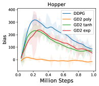
(a) Estimation bias

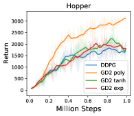
(b) Performance

Figure 2: (a) Value estimation bias comparison, (b) Performance comparison between GD2 with different activations (polynomial activation, tanh activation, and exponential activation) and DDPG. The experiment is conducted on Hopper-v2 environment (5 runs, mean $\pm$ standard deviation). Note that exp denotes exponential activation, poly denotes polynomial activation, and tanh denotes tanh activation.

The experimental result is presented in Fig 2, where we observe significant estimation reduction compared to DDPG with the aid of generalized-activated weighting operator with different activation functions in Fig 2(a). GD2 significantly outperforms DDPG with activations like polynomial functions, or tanh functions as shown in Fig 2(b). It is interesting to note that different activations have different performance and bias reduction effect on this task, e.g., polynomial activation has much less estimation bias and the best performance on Hopper-v2, which indicates that the optimal activation function is task-relevant or task-specific.

5.2 Generalized-activated weighting operator upon double critics

Generalized-activated weighting operator also helps with underestimation bias. Note that the direct application of generalized-activated weighting operator on the value estimation from two critics of TD3 would lead to larger underestimation bias because $\mathcal{T}_{GD2}(s^{\prime})=GA_{g}(Q_{i}(s^{\prime},a;\theta_{i}^{\prime});\bm{\psi})\leq\max_{a}Q_{i}(s^{\prime},a;\theta_{i}^{\prime})$ based on Theorem 1 where the right side is the value estimation by TD3. We therefore apply double actors and estimate the target value for critic $i$ by $y_{i}=r+\gamma\mathcal{T}_{GD3}(s^{\prime})$ as in SD3 (Pan et al. (2020)), where $\mathcal{T}_{GD3}=GA_{g}(\hat{Q}_{i}(s^{\prime},\pi(s^{\prime}));\bm{\psi})$ and $\hat{Q}_{i}(s^{\prime},a)=\min_{i=1,2}\{Q_{i}(s^{\prime},a;\theta_{i}^{\prime})\}$. In this way, we can get an estimator with less bias than GD2 as guaranteed by Lemma 3. Considering there exist integral in generalized-activated weighting operator, we rewrite $GA_{g}(\cdot)$ in terms of expectation with importance sampling to convert it into a manageable formula given by Eq. (6) as suggested in (Haarnoja et al. (2017)).

$$\mathbb{E}_{a^{\prime}\sim p}\left[\frac{g(\hat{Q}(s^{\prime},a^{\prime};\bm{\psi})\hat{Q}(s^{\prime},a^{\prime}))}{p(a^{\prime})}\right]{\Big{/}}\mathbb{E}_{a^{\prime}\sim p}\left[\frac{g(\hat{Q}(s^{\prime},a^{\prime};\bm{\psi})}{p(a^{\prime})}\right],$$ (6)

where $p(a^{\prime})$ is the Gaussian probability density function which depends on the clipped action values. The novel algorithm, Generalized-activated Deep Double Deterministic Policy Gradients (GD3) is shown in Algorithm 2.

A detailed computational graph description on the different updating process of TD3 and GD3 is available in Fig 3. The general network architecture of GD3 is similar to that of TD3 while the update process is different. TD3 directly uses the minimal value estimation from two critic networks (Clipped Double Q-learning) while GD3 gives the value function an activation to create a new distribution that indicates the importance of each Q value and uses it as weights over action space to get a softer value estimation.

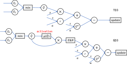
Figure 3: Graph describing the difference in updating between TD3 and GD3. E&N denotes Expectation and Normalization.

Algorithm 2 Generalized-activated Deep Double Deterministic Policy Gradients (GD3)

1:  Initialize critic networks $Q_{\theta_{1}},Q_{\theta_{2}}$ and actor networks $\pi_{\phi_{1}},\pi_{\phi_{2}}$ with random parameters $\theta_{1},\theta_{2},\phi_{1},\phi_{2}$; Initialize target network $\theta_{1}^{\prime}\leftarrow\theta_{1},\theta_{2}^{\prime}\leftarrow\theta_{2},\phi_{1}^{\prime}\leftarrow\phi_{1},\phi_{2}^{\prime}\leftarrow\phi_{2}$. Initialize replay buffer $\mathcal{B}=\{\}$.

2:  Given a non-decreasing function $g(\cdot;\bm{\psi})$ with parameter $\bm{\psi}$.

3:  for $t$ = 1 to $T$ do

4:     Select action $a$ with Gaussian exploration noise $\epsilon$, $\epsilon\sim\mathcal{N}(0,\sigma)$ based on current policy and observe reward $r$, new state $s^{\prime}$ and done flag $d$

5:     Store transitions, i.e. $\mathcal{B}\leftarrow\mathcal{B}\bigcup\{(s,a,r,s^{\prime},d)\}$

6:     for $i=1,2$ do

7:        Sample $N$ transitions $\{(s_{j},a_{j},r_{j},s_{j}^{\prime},d_{j})\}_{j=1}^{N}\sim\mathcal{B}$

8:        $a^{\prime}\leftarrow\pi_{\phi_{i}}(s^{\prime};\phi_{i}^{\prime})+\epsilon$, $\epsilon\sim$ clip($\mathcal{N}(0,\bar{\sigma}),-c,c$)

9:        $\hat{Q}(s^{\prime},a^{\prime})\leftarrow\min_{j=1,2}\left(Q_{j}(s^{\prime},a^{\prime};\theta_{j}^{\prime})\right)$

10:        Calculate $GA_{g}\left(\hat{Q}(s^{\prime},a^{\prime});\bm{\psi}\right)$ based on Eq.(6)

11:        $y_{i}\leftarrow r+\gamma(1-d)GA_{g}\left(\hat{Q}(s^{\prime},a^{\prime});\bm{\psi}\right)$

12:        Update critic networks: $\theta_{i}\leftarrow\arg\min_{\theta_{i}}\frac{1}{N}\sum_{s}(Q_{i}(s,a;\theta_{i})-y_{i})^{2}$

13:        Update actor networks: $\nabla J_{\phi_{i}}(\phi_{i})=\frac{1}{N}\sum_{s}\nabla_{a}Q_{i}(s,a;\theta_{i})|_{a=\pi_{\phi_{i}}(s;\phi_{i})}\nabla_{\phi_{i}}\pi(s;\phi_{i})$

14:        Update target networks: $\theta_{i}^{\prime}\leftarrow\tau\theta_{i}+(1-\tau)\theta_{i}^{\prime},\phi_{i}^{\prime}\leftarrow\tau\phi_{i}+(1-\tau)\phi_{i}^{\prime}$

15:     end for

16:  end for

Lemma 3.

The bias of GD3 is smaller than that of GD2, i.e., bias($\mathcal{T}_{GD3}$) $\leq$ bias($\mathcal{T}_{GD2}$).

Proof.

Suppose the activation function is identical for GD2 and GD3, and we denote it as $g(\cdot;\psi)$. We neglect the normalization term here as the integral of activated value function over action space gives similar results with identical activation function. There is no much difference between the value estimation from two critic networks. The bias of GD2 gives

$$bias(\mathcal{T}_{GD2})=\mathbb{E}\left[g(Q;\psi)Q(s,a^{\prime})\right]-\mathbb{E}\left[Q(s,\pi(s;\phi_{1}^{\prime});\theta^{\prime})\right],$$

where $\theta^{\prime}$ is the true parameter. GD3 uses two critic networks and it takes the minimal value estimation, i.e.,

$$\hat{Q}(s,\hat{a})=\min_{i=1,2}Q_{i}(s,\hat{a};\theta_{i}^{\prime}).$$

Obviously, $Q(s,a^{\prime})\leq\hat{Q}(s,\hat{a})$. Hence, the bias of GD3 gives

$$bias(\mathcal{T}_{GD3})=\mathbb{E}\left[g(\hat{Q};\psi)\hat{Q}(s,\hat{a}^{\prime})\right]-\mathbb{E}\left[Q(s,\pi(s;\phi_{i}^{\prime});\theta^{\prime})\right].$$

Because the activation function $g(\cdot;\psi)$ is non-decreasing, it is easy to find $g(Q(s,a^{\prime});\psi)\leq g(\hat{Q}(s,\hat{a});\psi)$. Therefore, $g(Q;\psi)Q(s,a^{\prime})\leq g(\hat{Q};\psi)\hat{Q}(s,\hat{a}^{\prime})$ which induce to the conclusion,

$$bias(\mathcal{T}_{GD3})\leq bias(\mathcal{T}_{GD2}).$$

∎

Lemma 3 paves the way for Theorem 3 which says that with proper activation function engineering satisfying Condition 1, it is ensured that we could find a suitable activation function which could result in softer value estimation, i.e., it would alleviate both large overestimation bias and underestimation bias. Many function families meet the constraint, e.g. exponential family, linear family, etc.

Condition 1.

$\int_{a\in\mathcal{A}}g(Q(s,a);\psi)Q(s,a)da\int_{a^{\prime}\in\mathcal{A}}1da^{\prime}\geq\int_{a\in\mathcal{A}}g(Q(s,a);\psi)da\int_{a^{\prime}\in\mathcal{A}}Q(s,a^{\prime})da^{\prime}.$

Theorem 3 (GD3 alleviates estimation bias).

Suppose that the actor is a local maximizer with respect to the critic, then there exists noise clipping parameter $c>0$ and some non-decreasing functions such that bias($\mathcal{T}_{TD3}$) $\leq$ bias($\mathcal{T}_{GD3}$) $\leq$ bias($\mathcal{T}_{DDPG}$).

Proof.

See Appendix A.2. ∎

Note that an additional positive bias term $b>0$ could lead to reduced bias as stated in the following corollary:

Corollary 2.

If some non-decreasing functions $g(\cdot;\bm{\psi})$ satisfy Condition 1, then a non-negative bias term would lead to a softer value estimation, i.e. the bias would be further reduced.

Proof.

Suppose the non-decreasing function $g(\cdot;\psi)$ satisfies Condition 1, let $b\geq 0$ be the bias term and denote $g^{\prime}(\cdot;\psi)=g(\cdot;\psi)+b$. Then,

$$bias(\mathcal{T}_{GD3}(s;g))-bias(\mathcal{T}_{GD3}(s;g^{\prime}))$$

$$=\mathbb{E}\left[GA_{g}(\hat{Q}(s,\cdot);\psi)\right]-\mathbb{E}\left[GA_{g^{\prime}}(\hat{Q}(s,\cdot);\psi)\right]$$

$$=\frac{\int_{a\in\mathcal{A}}g(Q;\psi)Q(s,a)da}{\int_{a^{\prime}\in\mathcal{A}}g(Q(s,a^{\prime});\psi)da^{\prime}}-\frac{\int_{a\in\mathcal{A}}(g(Q;\psi)+b)Q(s,a)da}{\int_{a^{\prime}\in\mathcal{A}}(g(Q(s,a^{\prime});\psi)+b)da^{\prime}}$$

$$=\frac{b\left(\int_{a\in\mathcal{A}}g(Q(s,a);\psi)Q(s,a)da\int_{a^{\prime}\in\mathcal{A}}1da^{\prime}\right)}{\int_{a^{\prime}\in\mathcal{A}}g(Q(s,a^{\prime});\psi)da^{\prime}\int_{a^{\prime}\in\mathcal{A}}(g(Q(s,a^{\prime});\psi)+b)da^{\prime}}-$$

$$\qquad\frac{b\left(\int_{a\in\mathcal{A}}g(Q(s,a);\psi)da\int_{a^{\prime}\in\mathcal{A}}Q(s,a^{\prime})da^{\prime}\right)}{\int_{a^{\prime}\in\mathcal{A}}g(Q(s,a^{\prime});\psi)da^{\prime}\int_{a^{\prime}\in\mathcal{A}}\left[g(Q(s,a^{\prime});\psi)+b\right]da^{\prime}}.$$

Since $b\geq 0$ and by using Condition 1, we get that

$$bias(\mathcal{T}_{GD3}(s;g))\geq bias(\mathcal{T}_{GD3}(s;g^{\prime})).$$

Thus, we get the conclusion that an additional non-negative bias term would lead to a softer value estimation. ∎

However, too large bias term is undesired based on the following corollary.

Corollary 3.

The Generalized-activated weighting operator approximates mean operator with sufficiently large bias term, i.e., $\lim_{b\rightarrow+\infty}GA_{g}(Q(s,\pi(s));\psi,b)=\mathbb{E}_{a\in\mathcal{A}}[Q(s,a)]$.

Proof.

By the definition of Generalized-activated weighting operator, if we add a bias term in the activation function, then

$$GA_{g}(Q(s,\pi(s));\bm{\psi},b)=\int_{a\in\mathcal{A}}\frac{(g(Q(s,a);\bm{\psi})+b)Q(s,a)}{\int_{a^{\prime}\in\mathcal{A}}(g(Q(s,a^{\prime});\bm{\psi})+b)da^{\prime}}da.$$

With sufficiently large bias term, the activation function would degenerate to constant function. It is then easy to conclude that $\lim_{b\rightarrow+\infty}GA_{g}(Q(s,\pi(s));\psi,b)=\mathbb{E}_{a\in\mathcal{A}}[Q(s,a)]$. ∎

Actually, an additional bias term is essential as the activation could be generalized to be non-decreasing in $(0,+\infty)$ instead of $\mathbb{R}$ as long as we perform a translation transformation, i.e., add a constant value such that the value function is non-negative. Hence the constraint is further loosened with a suitable bias term. However, too large bias term would equally weigh Q values, which may induce unsatisfying results (see Section 6.2). Furthermore, we experimentally find out that there is no need to strictly follow Condition 1 in practice as simple activations are adequate for a near-optimal estimation which is discussed in detail in Section 6.1.

6 Experiments

In this part, we conduct experiments on challenging MuJoCo (Todorov et al. (2012)) and Box2d (Catto (2011)) environments in OpenAI Gym (Brockman et al. (2016)) with simple activations. GD3 shares network configuration with the default setting of TD3. For the polynomial activation function, we mainly consider the index term $k$ to be 2 or 3 for simplicity. The coefficient $\alpha$ is mainly chosen from $\{0.01,0.05,0.5,0.1\}$. For the tanh and exponential activation, the coefficient $\beta$ is mainly chosen from $\{0.005,0.05,0.1\}$. The bias term $b$ for all activations is chosen from $\{0,1,2,5\}$ using grid search. All algorithms are run with 5 seeds and the performance is evaluated for 10 times every 5000 timesteps.

The network configuration for DDPG, TD3, and GD3 are similar, where we use fine-tuned DDPG instead of the vanilla DDPG as is suggested in (Fujimoto (2018)). The detailed hyperparameters for baseline algorithms and GD3 are shown in Table 1. We use the parameter suggested in (Fujimoto (2018)) for Humanoid-v2 where all algorithms fail if we use the same hyperparameters setup as other environments. We use the open-source implementation of SAC (Soft Actor Critic) in Github by the author (https://github.com/haarnoja/sac) where the hyperparameters are followed the same way as those in TD3 paper (Fujimoto et al. (2018)). The task-specific optimal activation parameter setup are shown in Table 2. Notice that the optimal activations are mostly polynomial, which indicates that fine-tuning the polynomial activation function can guarantee a satisfying performance on most of the tasks (see Fig 6 for more detailed performance of polynomial activation). It also reveals that simple activation functions are adequate for satisfying performance.

Hyperparameter	Humanoid-v2	Other tasks
Shared
Actor network	$(256,256)$	$(400,300)$
Critic network	$(256,256)$	$(400,300)$
Batch size	$256$	$100$
Learning rate	$3\times 10^{-4}$	$10^{-3}$
Optimizer	Adam
Discount factor	$0.99$
Replay buffer size	$10^{6}$
Warmup steps	$10^{4}$
Exploration noise	$\mathcal{N}(0,0.1)$
Noise clip	$0.5$
Target update rate	$5\times 10^{-3}$
TD3
Target update interval	$2$
Target nosie	$0.2$
GD3
Number of noises	$50$
Action noise variance	$0.2$

Table 1: Hyperparameters setup for baseline algorithms and GD3.

Environment	activation	coef	index	bias
Ant-v2	poly	$0.05$	$3$	$2$
BipedalWalker-v3	poly	$0.05$	$2$	$2$
HalfCheetah-v2	poly	$0.05$	$3$	$2$
Hopper-v2	poly	$0.05$	$2$	$2$
Humanoid-v2	poly	$0.05$	$2$	$2$
LunarLancerContinuous-v2	poly	$0.05$	$3$	$5$
Swimmer-v2	exp	—	$500$	$0$
Walker2d-v2	poly	$0.05$	$2$	$2$

Table 2: Hyperparameters setup for activations of GD3 in different environments. Note that coef denotes coefficient, poly refers to polynomial activations, and exp refers to exponential activations. Polynomial activation has hyperparameters of coefficient $\alpha$, index term $k$, bias term $b$, and exponential activation has hyperparameters of index term $\beta$ and bias term $b$.

6.1 How different activation functions perform?

Both GD2 and GD3 stand for a huge family of methods with activated weighting of any non-decreasing functions, which may lead to activation function engineering dilemma, i.e., it may be confusing what activation function to choose when dealing with an unknown environment. We claim that there is no need for trivial design (it is hard to design functions that meet the constraint in Condition 1), because we could get satisfying performance with some simple functions. We verify this by choosing three types of commonly used functions, polynomial function $g(x;\alpha,k,b)=\alpha x^{k}+b,\,(\alpha,k,b>0)$ and tanh $g(x;\beta,b)=\frac{\exp(\beta x)-\exp(-\beta x)}{\exp(\beta x)+\exp(-\beta x)}+b,\,(\beta,b>0)$, and exponential function $g(x;\beta,b)=\exp(\beta x)+b,(\beta,b>0)$, as activation function and testing the effectiveness of these activation functions under different parameters. The index term $k$ in polynomial activation is not required to be even as we would add a non-negative bias term. We select one typical environment in MuJoCo Todorov et al. (2012), Hopper-v2, to uncover the properties and benefits of simple activations. The detailed hyperparameter setup is listed in Table 1.

Can operator distance be bounded? Based on Theorem 1, the $T(Q^{*})$ term in the upper bound remains uncertain with arbitrary non-decreasing activations. Intuitively, if we assume $Q$ function is smooth, then $T(Q*)$ can be bounded as the activation function is non-decreasing and the $Q$ value is bounded. While it is essential to analyze whether the bound can be bounded with simple activation functions empirically. We run 5 independent experiments on Hopper-v2 with polynomial, tanh and exponential activations. It turns out that though poly and tanh deviate a little far away from max operator compared with exponential activation, the distance is actually measurable and it would gradually converge with the increment of training steps, which is shown clearly in Fig 4(a) where poly refers to polynomial activation. The distance between max operator and generalized-activated weighting operator is doomed to be bounded as larger Q values always get larger weights which makes the weighted value estimation lean to the maximal value with value iteration thanks to the non-decreasing activation function. The convergence ensures that our estimator is valid.

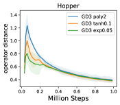
(a) Distance

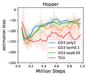
(b) Estimation bias

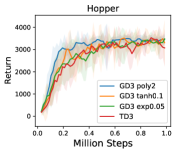
(c) Performance

Figure 4: Comparison among exponential activation, polynomial activation and tanh activation: (a) distance between activations and max operator; (b) value estimation bias; (c) overall performance with different activations (5 runs, mean $\pm$ standard deviation).

Can GD3 alleviate bias? Based on Theorem 3, we could get a suitable estimator that could achieve a balance between overestimation bias and underestimation bias with proper activation design. We verify whether simple activations could alleviate the bias by recording the bias induced by GD3 and comparing it with TD3. True values are evaluated by rolling out the present policy and averaging the discounted future rewards over the trajectories which start from the sampled states every $10^{5}$ steps. Activations help relieve overestimation bias as guaranteed by Corollary 1 but not necessarily underestimation bias, while we can find such function as long as it meets Condition 1. However, the result in Fig 4(b) shows that simple activation functions may induce larger bias than TD3 where all of the activations (polynomial, tanh, exponential) reserve larger bias than TD3. It indicates that simple activations can also empirically benefit underestimation bias alleviation. Fig 4(c) shows that simple activations are enough for good performance where all of them outperform TD3 on Hopper-v2.

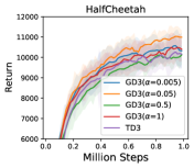
(a) The effect of coefficient $\alpha$.

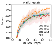
(b) The effect of index $k$.

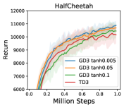
(c) The effect of $\beta$ in tanh.

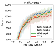
(d) The effect of $\beta$ in exp.

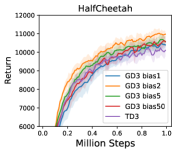
(e) The effect of bias $b$.

Figure 5: Parameter study and performance comparison. We use polynomial activation with $k=3$ in (a) and (e) (5 runs, mean $\pm$ standard deviation). Note that poly denotes polynomial activation, exp denotes exponential activation, and tanh denotes tanh activation.

6.2 How different parameters affect performance?

To better understand how hyperparameters in simple activation functions affect the performance of GD3, we conduct the parameter study in a MuJoCo environment, HalCheetah-v2. For polynomial activation, the coefficient $\alpha$ is vital as small $\alpha$ may lead to a slight underestimation bias while we could achieve an intermediate value that provides a trade-off as shown in Fig 5(a). The index $k$ in polynomial activation and $\beta$ in tanh activation significantly leverage the value estimation result where larger $k$ results in a smaller gap from the max operator. Fig 5(b) and Fig 5(d) show that too large $k$ in polynomial activation and too large $\beta$ in exponential activation may incur a bad performance. While there does exist a trade-off for $k$ in polynomial activation and $\beta$ in exponential activation. Fig 5(c) shows that smaller $\beta$ may be better for HalfCheetah-v2, and tanh is not sensitive to $\beta$ as long as it is not too large. From corollary 2, bias term is essential which could result in a softer value estimation while we should not use large bias as it may domain the activation function and lead to even weights (approximate mean operator according to Corollary 3). We should use a non-negative bias term to ensure the validity of activation such that larger values would always get larger weights. It turns out that we could achieve an intermediate trade-off for bias as shown in Fig 5(e). It is worth noting that almost all GD3 results under different parameters significantly outperform TD3.

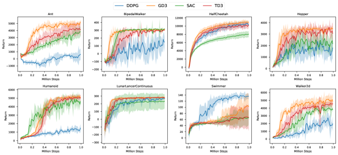
Figure 6: Performance comparison in continuous control tasks. The optimal activation functions are, Ant, HalfCheetah, LunarLancerContinuous: poly3; BipedalWalker, Hopper, Humaniod, Walker2d: poly2; Swimmer: exponential (5 runs, mean $\pm$ standard deviation). Most of the bias terms are set to be 2.

6.3 Extensive experiments

GD3 is designed for better value estimation where we get a soft value estimation that leans towards the max operator with a little gap by integrating the weighted value function over action space. To further investigate the benefits of simple activations, we conduct additional experiments on other environments. We use common baseline algorithms, DDPG (Lillicrap et al. (2015)), TD3 (Fujimoto et al. (2018)) and Soft Actor Critic (SAC) (Haarnoja et al. (2018)), as baselines where DDPG refers to fine-tuned DDPG in (Fujimoto (2018)) instead of vanilla DDPG implementation (as the vanilla DDPG performs badly). The result could be seen in Fig 6 where we find that GD3 significantly outperforms these common baseline methods with larger return and faster convergence. Notice that optimal activations for different tasks are actually task-specific. While polynomial activation performs well on almost all of the tasks. Various choices of activations make GD3 more flexible and changeable which makes it possible for near-optimal value estimation with reasonable activation functions.

7 Conclusion

We propose a general framework for bias alleviation in deep reinforcement learning, namely generalized-activated weighting operator. We show that the distance between generalized-activated weighting operator and max operator can be bounded both theoretically and empirically. We further present Generalized-activated Deep Double Deterministic Policy Gradients (GD3) algorithm. GD3 does a correction to the value estimation with function transformation over action space, leveraging any non-decreasing activation functions. We find that there is no need for trivial activation design to specifically meet the bias constraints as optimal activations are task-specific and simple activations are adequate for both higher sample efficiency and good performance. Experimental results on several challenging continuous control tasks show that GD3 with task-specific activations significantly outperforms the common baseline methods.

For future work, it would be interesting to apply the generalized-activated weighting operator in discrete regime. It would also be interesting to study how to accelerate the learning process of double actors and design a more efficient variant of the GD3 algorithm.

Appendix A Omitted proofs

A.1 Proof of Theorem 1

Proof.

The left hand side could be derived directly by definition:

$$GA_{g}(Q(s,\pi(s));\psi)$$ (7)

$$\quad\leq\int_{a\in\mathcal{A}}\frac{g(Q(s,a);\psi)}{\int_{a^{\prime}\in\mathcal{A}}g(Q(s,a^{\prime});\psi)da^{\prime}}\max_{\hat{a}}Q(s,\hat{a})da$$

$$\quad\leq\max_{a}Q(s,a)$$

As is in (Pan et al. (2020)) and (Fujimoto et al. (2018)), in order to show the right hand side, we would need the aid of log-sum-g operator, i.e.,

$$\mathrm{lsg}_{\psi}(Q(s,\pi(s));\beta)=\frac{1}{\beta}\ln\int_{a\in\mathcal{A}}g(Q(s,a);\psi)da.$$

Note here the activation is a generalized one instead of exponential function, if $\psi=\beta$ and $g(Q(s,a);\psi)=\exp(\psi Q(s,a))$, the lsg operator would become lse operator. Through a non-decreasing function $g(\cdot)$, the estimated $Q$ value is activated with a new density distribution $p_{\psi}(s,a)=\frac{g(Q(s,a);\psi)}{\int_{a^{\prime}\in\mathcal{A}}g(Q(s,a^{\prime}))da^{\prime}}$. Then from one perspective,

$$\mathrm{lsg}_{\psi}(Q(s,\pi(s)))-GA_{g}(Q(s,\pi(s));\psi)$$ (8)

$$=\frac{1}{\beta}\ln\int_{a\in\mathcal{A}}g(Q(s,a);\psi)da-\int_{a\in\mathcal{A}}p_{\psi}(s,a)Q(s,a)da$$

$$=\frac{1}{\beta}\int_{a\in\mathcal{A}}p_{\psi}(s,a)\left(\ln\frac{g(Q(s,a);\psi)}{p_{\psi}(s,a)}\right)da$$

$$\qquad\qquad-\int_{a\in\mathcal{A}}p_{\psi}(s,a)Q(s,a)da$$

$$=\frac{\int_{a\in\mathcal{A}}-p_{\psi}(s,a)\ln p_{\psi}(s,a)da}{\beta}+\int_{a\in\mathcal{A}}p_{\psi}(s,a)T(Q)da$$

$$\leq\frac{\int_{a\in\mathcal{A}1da-1}}{\beta}+T(Q^{*})$$

where $T(Q(s,a);\psi,\beta)=\frac{1}{\beta}\ln g(Q(s,a);\psi)-Q(s,a)$ and $T(Q^{*})$ is the maximum value of this function. The above inequality is induced by the fact that $\forall a$, $-p_{\psi}(s,a)\ln p_{\psi}(s,a)\leq 1-p_{\psi}(s,a)$ and $\int_{a\in\mathcal{A}}p_{\psi}(s,a)da=1$. Note that $\mathcal{C}(Q,s,\epsilon)\subset\mathcal{A}$, hence,

$$\mathrm{lsg}_{\psi}(Q(s,\pi(s)))$$ (9)

$$=\frac{\ln\int_{a\in\mathcal{A}}g(Q(s,a);\psi)da}{\beta}$$

$$\geq\frac{\ln\int_{a\in\mathcal{C}(Q,s,\epsilon)}g(\max_{a^{\prime}}Q(s,a^{\prime})-\epsilon;\psi)da}{\beta}$$

$$=\frac{\ln\int_{a\in\mathcal{C}}1da+\ln g(\max_{a^{\prime}}Q(s,a^{\prime})-\epsilon;\psi)}{\beta}$$

$$\geq\frac{\ln F(Q,s,\epsilon)+\ln\exp\left(\beta(\max_{a^{\prime}}Q(s,a^{\prime})-\epsilon)\right)}{\beta}$$

$$=\frac{\ln F(Q,s,\epsilon)}{\beta}+\max_{a^{\prime}}Q(s,a^{\prime})-\epsilon$$

We get the inequality that $\ln\int_{a\in\mathcal{A}}g(Q(s,a);\psi)da\geq\ln\int_{a\in\mathcal{C}(Q,s,\epsilon)}g(\max_{a^{\prime}}Q(s,a^{\prime})-\epsilon;\psi)da$ due to the fact that $g(\cdot)$ is a non-decreasing function, hence for $\forall\,Q\in\mathcal{C}(Q,s,\epsilon)$, $g(Q(s,a))\geq g(\max_{a^{\prime}}Q(s,a^{\prime}))$. Note that $\beta\in\mathcal{B}$, i.e. $\beta$ is small. By combining Eq.(8) and Eq. (9) and denote $M(Q,\epsilon;\psi,\beta)=\epsilon+\frac{\int_{a\in\mathcal{A}}1da-1+\ln F(Q,s,\epsilon)}{\beta}+T(Q^{*})$, we have the desired conclusion.

∎

A.2 Proof of Theorem 3

Proof.

By using Corollary 1 and Lemma 3, the right hand side can be easily shown. For the left hand side, if the non-decreasing function $g(Q(s,\pi(s);\theta^{-});\psi)$ satisfies Condition 2, then the left hand side holds.

Condition 2.

$\int_{a\in\mathcal{A}}g(Q(s,a);\psi)Q(s,a)da\int_{a^{\prime}\in\mathcal{A}}1da^{\prime}\geq\int_{a\in\mathcal{A}}g(Q(s,a);\psi)da\int_{a^{\prime}\in\mathcal{A}}Q(s,a^{\prime})da^{\prime}$

By definition, we have

$$bias(\mathcal{T}_{TD3}(s))=\mathbb{E}[\hat{Q}_{i}(s,a)]-\mathbb{E}\left[Q(s,\pi(s;\phi_{i}^{\prime});\theta^{\prime})\right]$$ (10)

where $\theta^{\prime}$ is the true parameter and the value estimation $\hat{Q}_{i}(s,a)=\min_{i=1,2}Q_{i}(s,a;\theta_{i}^{\prime})$.

$$bias(\mathcal{T}_{GD3}(s))=\mathbb{E}[GA_{g}(\hat{Q}_{i}(s,a);\psi)]-\mathbb{E}\left[Q(s,\pi(s;\phi_{i}^{\prime});\theta^{\prime})\right]$$ (11)

Eq. (10) and Eq. (11) have the same component. Thus,

$$bias(\mathcal{T}_{GD3}(s))-bias(\mathcal{T}_{TD3}(s))$$ (12)

$$\quad\quad=\mathbb{E}[GA_{g}(\hat{Q}_{i}(s,a);\psi)]-\mathbb{E}[\hat{Q}_{i}(s,a)]$$

If Condition 2 holds, we have $\frac{\int_{a\in\mathcal{A}}g(Q(s,a);\psi)Q(s,a)da}{\int_{a\in\mathcal{A}}g(Q(s,a);\psi)da}\geq\frac{\int_{a^{\prime}\in\mathcal{A}}Q(s,a^{\prime})da^{\prime}}{\int_{a^{\prime}\in\mathcal{A}}1da^{\prime}}$ which is exactly $\mathbb{E}[GA_{g}(\hat{Q}_{i}(s,a);\psi)]\geq\mathbb{E}[\hat{Q}_{i}(s,a)]$ and hence the left hand side holds.

It turns out that there exist some non-decreasing functions satisfying such inequality apart from softmax, e.g., the linear activation family. Suppose $g(Q(s,\cdot);\psi)=\psi Q(s,\cdot)+b$, $b\in\mathbb{R}$ and we require $b\geq 0$ here. Then we have the generalized-activated weighting operator: $GA_{g}(Q(s,\cdot);\psi)=\int_{a\in\mathcal{A}}\frac{(\psi Q(s,a)+b)Q(s,a)}{\int_{a^{\prime}\in\mathcal{A}}(\psi Q(s,a^{\prime})+b)da^{\prime}}da$. We also have $\psi\geq 0$ as the activation function has to be non-decreasing. By applying Cauchy-Schwarz inequality, it is easy to find

$$\quad\nabla_{\psi}GA_{g}(Q(s,\cdot);\psi)$$ (13)

$$=\nabla_{\psi}\int_{a\in\mathcal{A}}\frac{(\psi Q(s,a)+b)Q(s,a)}{\int_{a^{\prime}\in\mathcal{A}}(\psi Q(s,a^{\prime})+b)da^{\prime}}da$$

$$=\frac{b\left[\int_{a\in\mathcal{A}}Q^{2}(s,a)da\int_{a^{\prime}\in\mathcal{A}}1da^{\prime}-(\int_{a\in\mathcal{A}}Q(s,a)da)^{2}\right]}{\left(\int_{a^{\prime}\in\mathcal{A}}(\psi Q(s,a^{\prime})+b)da^{\prime}\right)^{2}}$$

$$\geq 0$$

Exponential family, i.e., $g(Q(s,\cdot);\psi,k)=k^{\psi Q(s,\cdot)},k\geq 1,\psi\geq 0,$ also satisfies the inequality, follow similar procedure as the above proof and apply Cauchy-Schwarz inequality, we have

$$\quad\nabla_{\psi}GA_{g}(Q(s,\cdot);\psi)$$ (14)

$$=\nabla_{\psi}\int_{a\in\mathcal{A}}\frac{k^{\psi Q(s,a)}Q(s,a)}{\int_{a^{\prime}\in\mathcal{A}}k^{\psi Q(s,a^{\prime})}da^{\prime}}da$$

$$=\frac{\ln k\left(\int_{a\in\mathcal{A}}Q^{2}(s,a)k^{\psi Q(s,a)}da\int_{a^{\prime}\in\mathcal{A}}k^{\psi Q(s,a)}da^{\prime}\right)}{(\int_{a^{\prime}\in\mathcal{A}}k^{\psi Q(s,a^{\prime})}da^{\prime})^{2}}$$

$$\quad-\frac{\ln k\left(\int_{a\in\mathcal{A}}Q(s,a)k^{\psi Q(s,a)}da\right)^{2}}{\left(\int_{a^{\prime}\in\mathcal{A}}k^{\psi Q(s,a^{\prime})}da^{\prime}\right)^{2}}$$

$$\geq 0$$

∎

JiafeiLyu.jpg Jiafei Lyu. Jiafei Lyu received his B.S. degree in Engineering Physics from Tsinghua University, Beijing, China, in 2020. He is currently pursuing a Ph.D. degree in Tsinghua Shenzhen International Graduate School. His research interest includes deep reinforcement learning, big data analysis, machine learning, and artificial intelligence.

yuyang.jpg Yu Yang. Yu Yang received his B.S. degree in Beijing Jiaotong University, Beijing, China, in 2020. He is currently a master student at Tsinghua Shenzhen International Graduate School. His research interest includes deep reinforcement learning, especially multi-agent deep reinforcement learning, deep learning, and artificial intelligence.

[width=2.5cm]jiangpengyan.jpg Jiangpeng Yan. Jiangpeng Yan received his B.S. degree in the Department of Automation from Tsinghua University, Beijing, China, in 2017. He is currently a Ph.D. Student in Department of Automation, Tsinghua University, China. His research interests include medical image analysis, reinforcement learning, and artificial intelligence.

xiuli.jpg Xiu Li. Xiu Li(Member, IEEE) received her Ph.D. degree in computer integrated manufacturing in 2000. Since then, she has been working with Tsinghua University. Her research interests are in the areas of data mining, deep learning, computer vision, reinforcement learning, and image processing.

References

- Arulkumaran et al. (2019) Arulkumaran, K., Cully, A., Togelius, J., 2019. Alphastar: an evolutionary computation perspective. Proceedings of the Genetic and Evolutionary Computation Conference Companion .
- Barth-Maron et al. (2018) Barth-Maron, G., Hoffman, M.W., Budden, D., Dabney, W., Horgan, D., Tb, D., Muldal, A., Heess, N., Lillicrap, T., 2018. Distributed distributional deterministic policy gradients. arXiv preprint arXiv:1804.08617 .
- Bellemare et al. (2017) Bellemare, M.G., Dabney, W., Munos, R., 2017. A distributional perspective on reinforcement learning, in: International Conference on Machine Learning, pp. 449–458.
- Brockman et al. (2016) Brockman, G., Cheung, V., Pettersson, L., Schneider, J., Schulman, J., Tang, J., Zaremba, W., 2016. Openai gym. arXiv preprint arXiv:1606.01540 .
- Catto (2011) Catto, E., 2011. Box2d: A 2d physics engine for games. URL: http://www.box2d.org .
- Cetin and Çeliktutan (2021) Cetin, E., Çeliktutan, O., 2021. Learning pessimism for robust and efficient off-policy reinforcement learning. ArXiv abs/2110.03375.
- Chen et al. (2021) Chen, Q., Jin, Y., Song, Y., 2021. Fault-tolerant adaptive tracking control of euler-lagrange systems — an echo state network approach driven by reinforcement learning. Neurocomputing .
- Ciosek et al. (2019) Ciosek, K., Vuong, Q., Loftin, R., Hofmann, K., 2019. Better exploration with optimistic actor critic, in: Advances in Neural Information Processing Systems, pp. 1787–1798.
- Fujimoto (2018) Fujimoto, S., 2018. Open-source implementation for td3. https://github.com/sfujim/TD3.
- Fujimoto et al. (2018) Fujimoto, S., Hoof, H., Meger, D., 2018. Addressing function approximation error in actor-critic methods, in: International Conference on Machine Learning, pp. 1587–1596.
- Gu et al. (2016) Gu, S., Lillicrap, T., Sutskever, I., Levine, S., 2016. Continuous deep q-learning with model-based acceleration, in: International Conference on Machine Learning, pp. 2829–2838.
- Haarnoja et al. (2017) Haarnoja, T., Tang, H., Abbeel, P., Levine, S., 2017. Reinforcement learning with deep energy-based policies, in: International Conference on Machine Learning, pp. 1352–1361.
- Haarnoja et al. (2018) Haarnoja, T., Zhou, A., Abbeel, P., Levine, S., 2018. Soft actor-critic: Off-policy maximum entropy deep reinforcement learning with a stochastic actor, in: International Conference on Machine Learning, pp. 1861–1870.
- van Hasselt et al. (2016) van Hasselt, H., Guez, A., Silver, D., 2016. Deep reinforcement learning with double q-learning, in: AAAI.
- He and Hou (2020) He, Q., Hou, X., 2020. Reducing estimation bias via weighted delayed deep deterministic policy gradient. ArXiv abs/2006.12622.
- Horgan et al. (2018) Horgan, D., Quan, J., Budden, D., Barth-Maron, G., Hessel, M., Van Hasselt, H., Silver, D., 2018. Distributed prioritized experience replay. arXiv preprint arXiv:1803.00933 .
- Huang et al. (2020) Huang, Q., Huang, R., Hao, W., Tan, J., Fan, R., Huang, Z., 2020. Adaptive power system emergency control using deep reinforcement learning. IEEE Transactions on Smart Grid 11, 1171–1182.
- Jiafei et al. (2021) Jiafei, L., Xiaoteng, M., Jiangpeng, Y., Xiu, L., 2021. Efficient continuous control with double actors and regularized critics. arXiv preprint arXiv:2106.03050 .
- Jiang and Lu (2021) Jiang, J., Lu, Z., 2021. Offline decentralized multi-agent reinforcement learning. ArXiv abs/2108.01832.
- Konda and Tsitsiklis (2000) Konda, V.R., Tsitsiklis, J.N., 2000. Actor-critic algorithms, in: Advances in neural information processing systems, pp. 1008–1014.
- Kuznetsov et al. (2021) Kuznetsov, A., Grishin, A., Tsypin, A., Ashukha, A., Vetrov, D.P., 2021. Automating control of overestimation bias for continuous reinforcement learning. ArXiv abs/2110.13523.
- Kuznetsov et al. (2020) Kuznetsov, A., Shvechikov, P., Grishin, A., Vetrov, D., 2020. Controlling overestimation bias with truncated mixture of continuous distributional quantile critics, in: International Conference on Machine Learning, pp. 5556–5566.
- Levine et al. (2020) Levine, S., Kumar, A., Tucker, G., Fu, J., 2020. Offline reinforcement learning: Tutorial, review, and perspectives on open problems. ArXiv abs/2005.01643.
- Lillicrap et al. (2015) Lillicrap, T.P., Hunt, J.J., Pritzel, A., Heess, N., Erez, T., Tassa, Y., Silver, D., Wierstra, D., 2015. Continuous control with deep reinforcement learning. arXiv preprint arXiv:1509.02971 .
- Liu et al. (2020) Liu, F., Tang, R., Guo, H., Li, X., Ye, Y., He, X., 2020. Top-aware reinforcement learning based recommendation. Neurocomputing 417, 255–269.
- Liu et al. (2021) Liu, S., Cao, J., Wang, Y., Chen, W., Liu, Y., 2021. Self-play reinforcement learning with comprehensive critic in computer games. Neurocomputing 449, 207–213.
- Ma et al. (2021) Ma, C., Zhang, J., Liu, J., Ji, L., Gao, F., 2021. A parallel multi-module deep reinforcement learning algorithm for stock trading. Neurocomputing 449, 290–302.
- Ma et al. (2020) Ma, X., Xia, L., Zhou, Z., Yang, J., Zhao, Q., 2020. Dsac: Distributional soft actor critic for risk-sensitive reinforcement learning. arXiv: Learning .
- Meng et al. (2020) Meng, L., Gorbet, R., Kulić, D., 2020. The effect of multi-step methods on overestimation in deep reinforcement learning. arXiv preprint arXiv:2006.12692 .
- Mirhoseini et al. (2020) Mirhoseini, A., Goldie, A., Yazgan, M., Jiang, J.W., Songhori, E.M., Wang, S., Lee, Y.J., Johnson, E., Pathak, O., Bae, S., Nazi, A., Pak, J., Tong, A., Srinivasa, K., Hang, W., Tuncer, E., Babu, A., Le, Q.V., Laudon, J., Ho, R., Carpenter, R., Dean, J., 2020. Chip placement with deep reinforcement learning. ArXiv abs/2004.10746.
- Mnih et al. (2016) Mnih, V., Badia, A.P., Mirza, M., Graves, A., Lillicrap, T., Harley, T., Silver, D., Kavukcuoglu, K., 2016. Asynchronous methods for deep reinforcement learning, in: International conference on machine learning, pp. 1928–1937.
- Mnih et al. (2015) Mnih, V., Kavukcuoglu, K., Silver, D., Rusu, A.A., Veness, J., Bellemare, M.G., Graves, A., Riedmiller, M., Fidjeland, A.K., Ostrovski, G., et al., 2015. Human-level control through deep reinforcement learning. nature 518, 529–533.
- Moskovitz et al. (2021) Moskovitz, T., Parker-Holder, J., Pacchiano, A., Arbel, M., Jordan, M., 2021. Tactical optimism and pessimism for deep reinforcement learning, in: Advances in Neural Information Processing Systems.
- Pálos and Huszák (2020) Pálos, P., Huszák, Á., 2020. Comparison of q-learning based traffic light control methods and objective functions. 2020 International Conference on Software, Telecommunications and Computer Networks (SoftCOM) , 1–6.
- Pan et al. (2020) Pan, L., Cai, Q., Huang, L., 2020. Softmax deep double deterministic policy gradients. Advances in Neural Information Processing Systems 33.
- Pei et al. (2019) Pei, C., Yang, X., Cui, Q., Lin, X., Sun, F., Jiang, P., Ou, W., Zhang, Y., 2019. Value-aware recommendation based on reinforcement profit maximization. The World Wide Web Conference .
- Popov et al. (2017) Popov, I., Heess, N., Lillicrap, T., Hafner, R., Barth-Maron, G., Vecerik, M., Lampe, T., Tassa, Y., Erez, T., Riedmiller, M., 2017. Data-efficient deep reinforcement learning for dexterous manipulation. arXiv preprint arXiv:1704.03073 .
- Silver et al. (2014) Silver, D., Lever, G., Heess, N., Degris, T., Wierstra, D., Riedmiller, M., 2014. Deterministic policy gradient algorithms, in: International Conference on Machine Learning, pp. 387–395.
- Silver et al. (2015) Silver, D., Schrittwieser, J., Simonyan, K., Antonoglou, I., Huang, A., Guez, A., Hubert, T., et al., 2015. Mastering the game of go without human knowledge. nature 550, 354–359.
- Singh et al. (1994) Singh, S.P., Jaakkola, T., Jordan, M.I., 1994. Convergence of stochastic iterative dynamic programming algorithms, in: Advances in Neural Information Processing Systems, pp. 703–710.
- Sutton et al. (2000) Sutton, R.S., McAllester, D.A., Singh, S.P., Mansour, Y., 2000. Policy gradient methods for reinforcement learning with function approximation, in: Advances in neural information processing systems, pp. 1057–1063.
- Todorov et al. (2012) Todorov, E., Erez, T., Tassa, Y., 2012. Mujoco: A physics engine for model-based control, in: 2012 IEEE/RSJ International Conference on Intelligent Robots and Systems, IEEE. pp. 5026–5033.
- Watkins and Cornish Hellaby (1989) Watkins, C., Cornish Hellaby, J., 1989. Learning from delayed rewards .
- Yang et al. (2021) Yang, Y., Ma, X., Li, C., Zheng, Z., Zhang, Q., Huang, G., Yang, J., Zhao, Q., 2021. Believe what you see: Implicit constraint approach for offline multi-agent reinforcement learning. ArXiv abs/2106.03400.
- Ye et al. (2020a) Ye, D., Chen, G., Zhang, W., Chen, S., Yuan, B., Liu, B., Chen, J., Liu, Z., Qiu, F., Yu, H., Yin, Y., Shi, B., Wang, L., Shi, T., Fu, Q., Yang, W., Huang, L., Liu, W., 2020a. Towards playing full moba games with deep reinforcement learning. ArXiv abs/2011.12692.
- Ye et al. (2020b) Ye, D., Liu, Z., Sun, M., Shi, B., Zhao, P., Wu, H., Yu, H., Yang, S., Wu, X., Guo, Q., Chen, Q., Yin, Y., Zhang, H., Shi, T., Wang, L., Fu, Q., Yang, W., Huang, L., 2020b. Mastering complex control in moba games with deep reinforcement learning. ArXiv abs/1912.09729.
- Zhang et al. (2017) Zhang, Z., Pan, Z., Kochenderfer, M.J., 2017. Weighted double q-learning., in: IJCAI, pp. 3455–3461.