AutoCTS: Automated Correlated Time Series Forecasting – Extended Version
Abstract.
Correlated time series (CTS) forecasting plays an essential role in many cyber-physical systems, where multiple sensors emit time series that capture interconnected processes. Solutions based on deep learning that deliver state-of-the-art CTS forecasting performance employ a variety of spatio-temporal (ST) blocks that are able to model temporal dependencies and spatial correlations among time series. However, two challenges remain. First, ST-blocks are designed manually, which is time consuming and costly. Second, existing forecasting models simply stack the same ST-blocks multiple times, which limits the model potential. To address these challenges, we propose AutoCTS that is able to automatically identify highly competitive ST-blocks as well as forecasting models with heterogeneous ST-blocks connected using diverse topologies, as opposed to the same ST-blocks connected using simple stacking. Specifically, we design both a micro and a macro search space to model possible architectures of ST-blocks and the connections among heterogeneous ST-blocks, and we provide a search strategy that is able to jointly explore the search spaces to identify optimal forecasting models. Extensive experiments on eight commonly used CTS forecasting benchmark datasets justify our design choices and demonstrate that AutoCTS is capable of automatically discovering forecasting models that outperform state-of-the-art human-designed models. This is an extended version of “AutoCTS: Automated Correlated Time Series Forecasting” (Wu et al., 2022), to appear in PVLDB 2022.
1. Introduction
We are witnessing continued developments in sensor technologies in cyber-physical systems (CPS), where sensors produce large amounts of correlated time series (Cirstea et al., 2018; Hu et al., 2018). For example, in transportation, traffic sensors embedded in roads emit multiple traffic time series that record traffic flows at their locations across time. Since the traffic on a road is often correlated with the traffic on nearby roads, the traffic time series are often correlated (Pedersen et al., 2020a). Forecasting on correlated time series plays an essential role in ensuring effective operation of CPSs, such as identifying trends, predicting future behavior (Cirstea et al., 2019), and detecting outliers (Campos et al., 2022). For instance, traffic time series forecasting can improve vehicle routing in transportation systems (Guo et al., 2020; Liu et al., 2018a; Pedersen et al., 2020b; Yang et al., 2020).
By considering both temporal dependencies in time series and spatial correlations among different time series, recent deep learning models demonstrate impressive and state-of-the-art performance on correlated time series forecasting. Temporal dependencies capture how historical values influence future values. We use the term “spatial correlations” because the correlations among time series are often due to the proximity of the locations in which the sensors that generate the time series are deployed, but correlations may also be due to other factors. More specifically, correlated time series are modeled as a spatio-temporal (ST) graph, where nodes represent time series, and edges represent spatial correlations between pairs of time series (Cirstea et al., 2021; Wu et al., 2020).
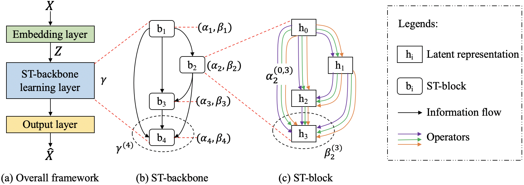
Based on the above ST-graph modeling, different models are proposed to enable forecasting. Figure 1(a) summarizes existing forecasting models, which often include (1) an embedding layer that transforms the input time series data, (2) a ST-backbone that consists of a stack of multiple ST-blocks that are able to extract appropriate spatio-temporal features from the embedded time series data, and (3) an output layer that produces a final forecasting based on the features extracted by the ST-backbone.
Different studies propose unique ST-blocks that are responsible for the capture of both the temporal dependencies and spatial correlations (Yu et al., 2018; Li et al., 2018; Guo et al., 2019; Wu et al., 2019; Zheng et al., 2020; Diao et al., 2019; Fang et al., 2019; Li and Zhu, 2021; Xu et al., 2020; Cirstea et al., 2019; Hu et al., 2020). For example, STGCN (Yu et al., 2018) employs a “sandwich” ST-block that includes two temporal convolutions, which model temporal dependencies, with one graph convolution in-between, which captures spatial correlations; and Graph Wavenet (Wu et al., 2019) uses a simpler ST-block that first employs gated temporal convolution to model temporal dependencies and then uses graph convolution to capture spatial correlations.


Although various forecasting models have been proposed and the state-of-the-art accuracy continues to improve, two major limitations remain.
Manually Designed ST-blocks. Existing studies rely on human expertise to design effective ST-blocks, which is both inefficient, often taking weeks or months, and costly. In addition, as a large number of operators exist that are able to capture temporal dependencies (i.e., T-operators) and spatial correlations (i.e., S-operators), the search space for designing ST-blocks is very large. Thus, it is almost impossible for humans to be able to identify an optimal combination of T/S-operators, thus potentially missing ST-blocks with high effectiveness. Further, rapid developments in machine learning are likely to lead to the invention of new, competitive operators. In order to benefit from new operators, it is necessary to reiterate the inefficient and costly manual design process whenever a new operator becomes available. Next, since time series from different domains have different characteristics, it is very difficult to design an ST-block that works well on substantially different datasets. To contend with these limitations, an automated design process that is able to identify optimal ST-blocks from a configurable search space of T/S-operators for specific datasets is called for.
ST-backbone with Stacking, Homogeneous ST-blocks. Existing forecasting models often have an ST-backbone that stacks the same ST-blocks sequentially multiple times to achieve “deeper” models that are better at capturing complex dependencies and correlations, as shown in Figure 1(a). We hypothesize that ST-backbones with heterogeneous ST-blocks connected by more flexible topologies, as exemplified in Figure 1(b), hold the potential to yield higher accuracy. Here, different ST-blocks, instead of same ST-blocks, can be connected using arbitrary topologies rather than by sequential stacking only. Intuitively, different ST-blocks may extract distinct features, which may enable more diverse and thus potentially better representations of time series. Supporting multiple topologies offers added flexibility, thus contributing further to enabling diverse models, which may enhance accuracy and stability. However, considering topologically flexible, heterogeneous ST-blocks increases the search space when designing forecasting models, thus rendering manual design more difficult and time-consuming. This naturally calls for an automated design approach.
Although Neural Architecture Search (NAS), a technology that automatically learns neural architectures (Elsken et al., 2019), is able to outperform human-designed architectures on various tasks in computer vision (CV) (Pham et al., 2018; Liu et al., 2018b) and natural language processing (NLP) (Wang et al., 2020), existing NAS methods fail to offer automated solutions capable of solving the aforementioned two limitations. First, no well-defined search space exists for correlated time series forecasting, as existing NAS methods often focus on CV and NLP. Directly using the search space designed for other domains fails to identify ST-blocks with high potential for capturing both temporal dependencies and spatial correlations. Directly using all existing S/T-operators in the literature yields an extremely large search space, thus making it very difficult and time-consuming to identify promising ST-blocks. Second, most existing NAS methods focus on identifying an optimal cell, e.g., an ST-block in our setting, while assuming a fixed topology, e.g., stacking the same ST-blocks as shown in Figure 1(a), for connecting multiple instances of the same cell to derive the final model (Elsken et al., 2019; Zoph et al., 2018; Pham et al., 2018; Liu et al., 2018b). This fails to address the second limitation of manually designed forecasting models.
We propose AutoCTS that is able to not only automatically design ST-blocks but also ST-backbones with complex topologies that connect heterogeneous ST-blocks, thus addressing the two limitations. To create AutoCTS, we first design a micro search space targeting ST-blocks that models operators and how different operators are connected using a graph. To enable effective and efficient search, we judiciously select a compact set of T-operators that model temporal dependencies and S-operators that model spatial correlations based on a thorough analysis of existing, manually designed ST-blocks. This enables us to automatically identify highly competitive ST-blocks in the proposed micro search space, thus addressing the first limitation. Next, we propose a macro search space, along with a joint search strategy that allows searches for an optimal topology among heterogeneous ST-blocks. This addresses the second limitation.
To the best of our knowledge, this is the first study that systematically investigates automated correlated time series forecasting by exploring jointly the neural architectures of ST-blocks and ST-backbones. The study makes three contributions. First, we carefully design a micro search space for correlated time series forecasting, including both T-operators and S-operators, along with a search strategy that is able to identify optimal ST-blocks from the micro search space. Second, we propose a macro search space, along with a joint search strategy that searches both ST-blocks and forecasting models, while allowing flexible topologies among heterogeneous ST-blocks. Third, we conduct extensive experiments on correlated time series from different application domains to offer insight into and justify our design choices, demonstrating also that our proposal is able to outperform state-of-the-art methods.
The remainder of the paper is organized as follows. Section 2 presents preliminaries. Section 3 elaborates the proposed AutoCTS framework. Section 4 presents the empirical study. Section 5 covers related work, and Section 6 concludes and suggests future work.
2. Preliminaries
We introduce correlated time series forecasting, cover concepts that are necessary for the paper’s proposal, and formalize the problem.
Correlated Time Series. Consider correlated multivariate time series , where each time series covers timestamps and each timestamp is associated with features. For example, assuming that 100 sensors are deployed in a road network and each sensor reports both travel speed and traffic flow every 5 minutes. Then, for one day, we have correlated time series with time series covering timestamps and features. We use to indicate the -th time series, where , and to indicate the features from all time series at timestamp , where .
To model spatial correlations among different time series, we introduce a graph , where each vertex in corresponds to a time series so that , edges in represent spatial correlations between different time series, and adjacency matrix contains edge weights that reflect the strengths of the spatial correlations between time series. The edge weights are either predefined, e.g., based on the distances between the locations of the sensors that generate the time series (Li et al., 2018; Wu et al., 2019; Song et al., 2020), or learned in a data-driven manner (Bai et al., 2020; Wu et al., 2020; Cirstea et al., 2021).
Correlated Time Series Forecasting. We consider both single-step and multi-step correlated time series forecasting. Given the past steps, (1) for the single step forecasting, we predict the -th future step, where ; (2) for the multi-step forecasting, we predict a total of future steps, with . Formally, we define the single-step correlated time series forecasting problem as follows:
| (1) |
where is a forecasting model and is its learnable parameters; and represents forecasted values. Likewise, the multi-step correlated time series forecasting problem is defined as follows:
| (2) |
Problem Definition. The goal of the paper is to automatically identify an accurate forecasting model . This includes the identification of (1) architecture parameters that describe the model , e.g., which operators that are used in different ST-blocks and how the different ST-blocks are connected in the ST-backbone; and (2) model parameters that are used in the different operators, e.g., kernels in convolution operators and the projection matrices in attention operators. The objective function is show in Equation 3.
| (3) |
where returns the forecasting error of the model that is learned on a training dataset .
3. Automated CTS Forecasting
Figure 2 offers an overview of the automated CTS forecasting framework AutoCTS, which consists of three main components—an embedding layer, an ST-backbone learning layer, and an output layer.
The embedding layer maps the original input feature from time series to a high-dimensional representation , which facilities extracting richer features from the input time series.
The ST-backbone learning layer, which is the core component of AutoCTS, is able to automatically design ST-backbones that encompass heterogeneous ST-blocks (as exemplified in Figure 2 (b)), where the design of the heterogeneous ST-blocks is also automated (as exemplified in Figure 2 (c)). When searching for ST-backbones, we use parameter to parameterize the connections among different ST-blocks. For example, controls how the three connections from ST-blocks , , and connect to ST-block . When searching for ST-blocks, we search both (1) the operators between two representations, parameterized by , and (2) the different possible connections among different hidden representations, parameterized by . For example, represents the operators between hidden representations and in ST-block , represents, in ST-block , how the hidden representations , , and connect to the hidden representation . We use unique sets of parameters such that heterogeneous ST-blocks can be identified. The automatically designed ST-backbone takes as input the high-dimensional representation from the embedding layer and extracts spatio-temporal features, which are fed to the output layer.
Finally, the output layer makes the forecasting . We use a loss function, e.g., mean squared error, to measure the discrepancy between the forecast w.r.t. the ground truth to enable learning.
In the following, we first identify an appropriate search granularity (in Section 3.1), then we introduce the design of a micro search space for ST-blocks (in Section 3.2) and a macro search space for ST-backbones (in Section 3.3). Finally, we present the search strategy that explores the micro and macro search spaces jointly to discover promising forecasting models (in Section 3.4).
3.1. Search Granularity
The search space can be constructed from operators of different granularities. A search space based on fine-granularity operators offers more flexibility and greater opportunities for identifying promising neural architectures that cannot be identified by human experts, but it often also yields a very large search space, the search of which takes prohibitively long time and requires excessive computational resources. In contrast, a search space based on coarse-granularity operators yields a smaller search space and thus speeds up the search process, but it may also introduce human biases that may prevent the identification of high-performance architectures.
More specifically, in our problem setting, three different granularities exist. From coarse to fine, they are ST-blocks, S/T operators, and basic computations. We proceed to introduce the three granularities using a concrete example. Then, we discuss our design choices related to choosing the appropriate search granularity.
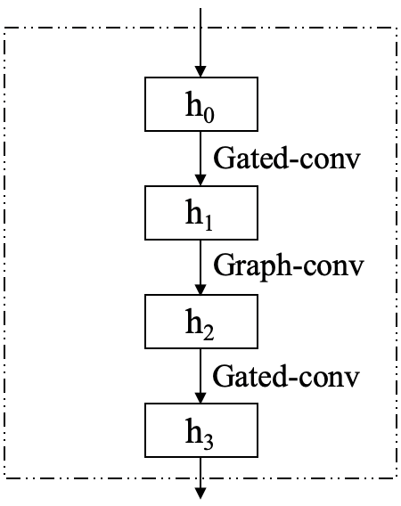
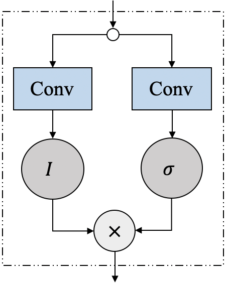
Figure 3 shows the neural architecture of Spatio-Temporal Graph Convolutional Networks (STGCN) (Yu et al., 2018), a human designed forecasting model. The backbone of STGCN consists of two ST-blocks that are stacked (cf. Figure 3(a)). An ST-block consists of three S/T operators—two T-operators, i.e., gated convolution operators, with an S-operator in-between, namely a graph convolution operator, (cf. Figure 3(b)). An S/T operator often consists of multiple basic computations. For example, Figure 3(c) shows the architecture of gated convolution, i.e., the T-operator. Here, and refer to an identity and a sigmoid function, respectively; is the convolution operator, and is the element-wise product. These are all basic computations.
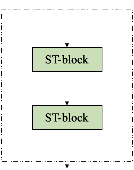
Based on the above, the coarsest search granularity is to use existing, manually-designed ST-blocks as atomic search units in the search space for finding novel ST-backbones. For example, instead of using a stacking structure with homogeneous ST-blocks as shown in Figure 3(a), it is possible to search for an ST-backbone with a more flexible structure with many different human designed ST-blocks as shown in Figure 1(b). However, since human designed ST-blocks may contain human biases already, only searching the different connections among them may limit the opportunities for finding novel and high-performance backbones.
The next granularity is that of using, human designed S/T-operators as atomic search units to search for novel ST-blocks. Since S/T-operators are at a finer granularity than ST-blocks, this granularity offers greater opportunities for discovering more powerful forecasting models that go beyond existing human designed models. In addition, whenever a new S/T-operator is designed, the new S/T-operator can be easily included in the search space. We consider this as an appropriate granularity.
The finest search granularity is to use basic operations as atomic search units to search for novel S/T operators. However, this leads to a much larger search space than when using S/T operators as the search space unit, incurs excessive computational costs, and requires a very large dataset to enable effective training (Mei et al., 2019).
To find highly competitive forecasting models without requiring high computational and memory costs, we choose to use S/T operators as the atomic search units in a so-called micro search space to discover novel ST-blocks. Next, in the macro search space, we use the automatically learned ST-blocks as atomic search units to identify novel ST-backbones with flexible structures.
3.2. Micro Search Space
The micro search space defines the possible architectures of the ST-blocks that can be discovered. We first introduce the design of the micro search space and then explain how to reduce the size of the micro search space to speed up search.
3.2.1. Micro-DAG
We assume that an ST-block includes latent representations. The first latent representation is the output representation from the embedding layer or the output representation of another ST-block. In addition, we consider a set of operators, e.g., including multiple S/T operators, that are able to transform one latent representation to a new latent representation.
We represent the micro search space as a directed acyclic graph, denoted as micro-DAG (see Figure 4). The micro-DAG has nodes , , that each denotes a latent representation. Node denotes the representation returned by the embedding layer. For each node pair , we have edges, where each edge corresponds to an operator from operator set . Figure 4(a) shows an example, where includes three operators such that each node pair is associated with three edges. In addition, we only include edges from node to if . This makes the graph a DAG, which simulates the forward flow when training a neural network.
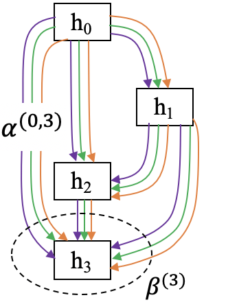
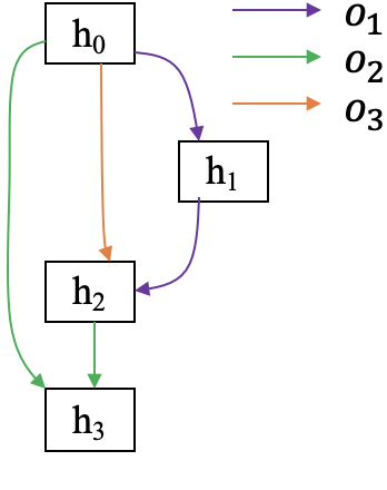
Figure 4(b) shows a derived ST-block, which is a subgraph of the micro-DAG. Specifically, the derived ST-block only retains one edge, i.e., one operator, between each node pair . In addition, for each node, it preserves at most two incoming edges. This enables relatively complex internal topologies for ST-blocks and avoids introducing too many parameters.
The micro-DAG represents all possible architectures of an ST-block with latent representations. This design yields to possible ST-blocks. This is because a micro-DAG with nodes has node pairs , where , and because each node pair can be connected by an operator from . In Section 3.2.3, we discuss how to select a compact operator set , thus reducing the size of the micro search space without comprising effectiveness.
3.2.2. Parameterizing ST-blocks
In order to derive an optimal ST-block, we introduce two sets of architecture parameters and , where parameterizes node pair and parameterizes nodes.
First, we parameterize each node pair with vector to indicate the weights over all operators in . Then transformation from node to node is formulated as a weighted sum of all operators.
| (4) |
where represents the weight of operator , which is to be learned, and is the representation after applying operator to representation .
Next, we parameterize each node based on its incoming edges. We use another architecture parameter to assign weights to the incoming edge groups at node , where each incoming edge group represents a hidden representation from a node that appears earlier than , i.e., . For example, in Figure 4, node has three incoming edge groups from , , and , respectively. We then apply a softmax function to normalize the parameter. If , it means that the weights of the representations from , , and are 0.3, 0.3, and 0.4, respectively. Therefore, for each node , we can compute its representation as the weighted sum of all transformations of its predecessor nodes.
| (5) | ||||
| (6) |
where is the architecture parameter value for weighting the transformation from to , which is to be learned.
In this way, given the first node , we are able to compute the representations of the remaining nodes in the micro-DAG. We use the representation of the last node as the output of the micro-DAG, and we thus feed to the output layer. This gives a forecasting model that we can train using classic back propagation. The training enables us to identify the most appropriate and .
After training, we derive the final ST-block. For each node pair , we compute a weight using Eq. 7 for each operator , and retain the operator with the largest , i.e., .
| (7) |
Next, for each node , we preserve two operators. One is the operator from node , i.e., its immediate predecessor node. The other one is the operator with the largest among the remaining operators, i.e., . For example, in Figure 4(b), always connects to , where . For , assuming , then is connected to .
| Family | Operator | Literature | Equation | |
| T-Operators | CNN | 1D Convolution | (Guo et al., 2019) | (8) |
| Gated Dilated Causal Convolution | (Yu et al., 2018; Diao et al., 2019; Huang et al., 2020) | (9) | ||
| (GDCC) | ||||
| RNN | Long Short Term Memory (LSTM) | (Lai et al., 2018; Shih et al., 2019) | (10) | |
| Gated Recurrent Unit (GRU) | (Li et al., 2018; Chen et al., 2020; Bai et al., 2020) | (11) | ||
| Attention | Transformer | (Park et al., 2020; Xu et al., 2020) | (12) | |
| Informer (INF-T) | (Zhou et al., 2021) | (13) | ||
| S-Operators | GCN | Chebyshev GCN | (Yu et al., 2018; Guo et al., 2019; Diao et al., 2019; Fang et al., 2019; Huang et al., 2020) | (14) |
| Diffusion GCN (DGCN) | (Li et al., 2018; Wu et al., 2019; Pan et al., 2021) | (15) | ||
| Attention | Transformer | (Park et al., 2020; Xu et al., 2020) | (16) | |
| Informer (INF-S) | None | (17) |
Reducing the gap between the micro-DAG and the derived ST-block. Due to how we reduce a micro-DAG to an ST-Block, there may be a large gap between the micro-DAG and the derived ST-Block, which may make the derived ST-block suboptimal. In other words, although we have learned an effective micro-DAG, the derived ST-block may not perform as well as the micro-DAG since the derived ST-Block can be very different from the micro-DAG.
Figure 5(a) shows an example. After training the micro-DAG, we get weight vector . To derive the ST-block, we retain the operator with the largest weight, e.g., the second operator. However, the other two operators have relatively high weights as well, meaning that they also contribute significantly to the transformation from to . In contrast, in the derived ST-block, only the second operator contributes to the transformation. This represents a big gap, which makes the derived ST-block may not be optimal.
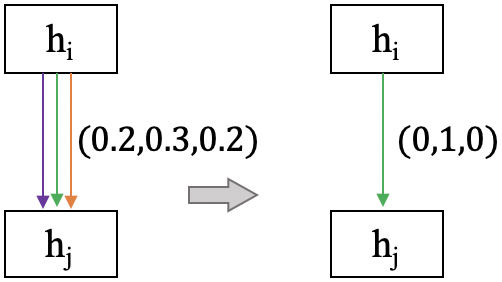
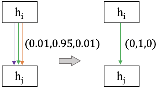
To reduce the discrepancy between the derived ST-block and the extended micro-DAG, we introduce a temperature parameter to the function when normalizing parameter , where we replace by . Thus, is computed as follows.
When , the output of is getting closer to a one-hot vector. In this way, for each node pair , the operator with largest is dominant, thus making it very close to the derived ST-block that only retains the operator with the largest weight. Figure 5(b) shows an example with a small gap when using the temperature parameter . In the micro-DAG, the 2nd operator plays a dominant role for the transformation from to , and the other two operators contribute only slightly. Thus, when ignoring the other two operators in the derived ST-block, the gap is insignificant. This ensures that the micro-DAG with optimal architecture parameters and is able to derive a high-performance ST-block.
In practice, if we set the temperature to be very small from the beginning, the training process can be unstable. Therefore, we set the initial value of to be relatively large, and perform exponential annealing on to reduce it gradually as training epochs increase.
3.2.3. Reducing Operator Set
Rather than using all S/T operators in the literature, we propose two principles to select a compact set of S/T operators to construct with the aim of achieving high search efficiency without compromising accuracy. First, selecting S/T operators that capture different perspectives is purposeful. To this end, we categorize existing S/T operators according to their characteristics. Second, for each category of S/T operators, we choose the most effective variant. This helps reduce operator set without losing promising operators.
We categorize commonly used S/T operators for correlated time series forecasting in Table 1. Specifically, we categorize the T-operators into three families—the Convolutional Neural Network (CNN) family, the Recurrent Neural Network (RNN) family, and the Attention family; and we categorize the S-operators into two families—the Graph Convolution Network (GCN) family and the Attention family.
For all equations in Table 1, denotes the input tensor and denotes the output tensor after applying an S/T operator to . Here, represents the number of time series or nodes in the graph, and represent the number of timestamps, and and represent the number of features. We use to represent the input and output of the -th time series and to represent the input and output of the -th timestamp. We use to represent the adjacency matrix; denotes convolution kernels; , , and represent projection matrices used in computing attention scores; and represent the diagonal in-degree and out-degree matrices, respectively; and is the Chebyshev polynomial of the adjacency matrix. Finally, is the convolution operator, represents the sigmoid function, is a sampling function used in Informer, and is the element-wise product.
Applying Principle 1: We analyze the different perspectives of different families for T-operators and S-operators, respectively. For T-operators, we consider two perspectives—(i) the ability of modeling long-term temporal dependencies and (ii) efficiency. Since short-term temporal dependencies can be relatively easily captured by all families, we do not consider it as a perspective. Figure 6 shows the CNN, RNN, and Attention families w.r.t. the two perspectives.
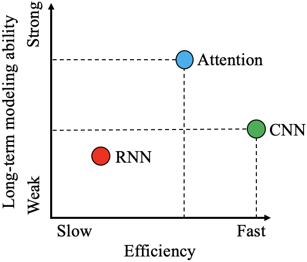
For the CNN family, the core operation is to convolve multiple kernels, e.g., matrices or vectors, with different parts of to extract meaningful features. The kernel size is often set to be small, which leads to a small receptive field that considers only local features and limits its ability of modeling long-term temporal dependencies. To model long-term temporal dependencies, it is possible to stack multiple CNN layers to expand the receptive filed (Wu et al., 2019, 2020; Kieu et al., 2018). Since convolutions at different parts of the input tensors are independent, CNNs can be easily parallelized and thus being very efficient.
For the RNN family, the core operation is to compute a hidden state for each timestamp . Since is computed based on , i.e., the hidden state from the previous timestamp , such recursive computations cannot be parallelized. Thus, RNN is inefficient. To model long term dependencies, many RNN computations need to be done sequentially. This makes RNN suffer from gradient vanishing and exploding problems (Khandelwal et al., 2018), making RNN difficult to capture long-term dependencies. Some recent studies have shown that CNN is able to outperform RNN in capturing long-term dependencies (Kalchbrenner et al., 2016; Oord et al., 2016; Gehring et al., 2017). This explains why RNN is placed lower than CNN in Figure 6.
For the Attention family, the core operation is, for each timestamp, to compute an attention score with each other timestamp. Then, a weighted sum based on the attention scores can be computed. Since the attention scores are computed w.r.t. all timestamps, this enables the Attention family to be very good at capturing long-term temporal dependencies. In addition, since the attention score computations for different timestamps are independent, they can be easily parallelized and thus being efficient. However, the CNN family has better efficiency than the Attention family in practice.
To conclude the discussion on the T-operators, we disregard the RNN family from our search space because CNN and Attention are more efficient and capture long-term temporal dependencies better. We keep both the CNN and Attention families because one is not better than the other one on both perspectives. We provide empirical evidence to justify this design choice in Section 4.
We proceed to analyze three different perspectives for the S-operators—(i) whether an adjacency matrix is required, (ii) the ability of capturing time-varying spatial correlations, and (iii) efficiency.
The GCN family relies on an adjacency matrix that indicates the neighboring nodes of each node. The adjacency matrix is often constructed based on meta information, e.g., the distances among the sensors which produce the time series or is learned from data (Wu et al., 2019; Bai et al., 2020). Given an adjacency matrix, for each node, graph convolution convolves features of neigboring nodes using a learnable kernel such that the features from the neighbors are aggregated. The aggregations per node are independent and thus can be done in parallel. As a result, GCN is efficient. The spatial correlations between two time series can be different across time, e.g., the correlations on two roads’ traffic time series in peak vs. offpeak hours. However, the adjacency matrix is often constructed based on distance that does not change across time, this makes GCN fail to capture dynamic spatial correlations.
The Attention family computes attention scores w.r.t. all other nodes for each node. Thus, it does not require an adjacency matrix that indicates the neighboring relationships. Next, the attention scores can be computed based on hidden representations at different timestamps, and thus it is able to capture time-varying dependencies. In terms of efficiency, attention scores at different nodes are independent and thus are parallelizable and efficient.
Table 2 summarizes the GCN vs. Attention families w.r.t. the perspectives of interest. We observe that the two families complement each other and thus we keep both families in our search space.
| Perspectives | GCN | Attention |
|---|---|---|
| Needs predefined adjacency matrix | Yes | No |
| Captures time-varying spatial correlations | No | Yes |
| Efficiency | Fastest | Fast |
Applying Principle 2: After determining the relevant S/T operator families, we apply the second principle to choose the most effective variant for each family. To do so, we consider two scenarios. If there exist studies that compare the different variants in the same experimental setting, we then directly choose the most effective variant. If such studies do not exist, we conduct experiments to identify the most effective variant.
For the CNN family, we consider 1D Convolution and Gated Dilated Causal Convolution (GDCC). The computations of both operators are shown in Equations 8 and 9 in Table 1, which clearly indicates that GDCC is an enhanced version of 1D convolution. In addition, a recent paper (Dauphin et al., 2017) has shown strong empirical evidence that GDCC is more effective than 1D convolution. Thus, for the CNN family, we include only GDCC into operator set .
For the temporal Attention family, we have two candidates— Transformer (Vaswani et al., 2017) and its more efficient variant, Informer (Zhou et al., 2021). Informer improves the attention mechanism in Transformer by only sampling a subset of timestamps to calculate the attention score with all the other timestamps, denoted by in Equation 13. In addition, Informer has been shown to be able to also achieve more accurate forecasting than Transformer on time series forecasting tasks (Zhou et al., 2021). Thus, we include only Informer, denoted by INF-T as it concerns temporal dependencies, into .
For the GCN family, we consider Chebyshev GCN (Kipf and Welling, 2017) and Diffusion GCN (Li et al., 2018). Although the two variants are commonly used in the literature, there is no existing studies compare the two variants in a consistent experimental setting for CTS forecasting. We thus design an experiment to compare them. This experiment is conducted on two datasets, namely METR-LA and PEMS03 (see the deatils of the two datasets in Section 4.1). The results in Table 3 show that the diffusion GCN consistently outperforms the Chebyshev GCN. Therefore, we include only diffusion GCN into .
| DGCN | Cheby GCN | Informer | Transformer | |
|---|---|---|---|---|
| METR-LA | 3.33 | 3.42 | 3.64 | 3.65 |
| PEMS03 | 18.44 | 21.55 | 23.79 | 23.54 |
For the spatial Attention family, only Transformer is used in the literature. However, since Informer achieves better accuracy on modeling temporal dependencies, it motivates us to consider it on modeling spatial correlations. We thus conduct an experiment to compare them. Table 3 shows that they have similar accuracy. Since Informer is more efficient than Transformer, we include Informer, denoted by INF-S as it concerns spatial correlations, into .
To summarize, we include GDCC, INF-T, DGCN, and INF-S as the S/T operators in our micro space. In addition, we also include two non-parametric operators, zero and identity. This yields a compact operator set with 6 operators.
3.3. Macro Search Space
We design a macro search space to search for topologies among different ST-blocks. This enables AutoCTS to generate ST-backbones with heterogeneous ST-blocks connected by flexible topologies.
Specifically, we represent the macro search space as a macro-DAG with nodes, where each node , , represents an ST-block, and an edge stands for information flow from node to node (see Figure 7(a)). Note that the predecessor of node is the embedding layer. An information flow from to means that the output representation of ST-block is fed into as the input representation of ST-block . This is different from the micro-DAG, where an edge indicates some operators that transform the representations.
In addition to the information flows which are to be learned, we also have hard code connections from all ST-blocks to the output layer. In other words, no matter which topology is learned to connect the ST-blocks, the outputs of all ST-blocks are merged and fed to the output layer.
The final, learned ST-backbone is a subgraph of the macro-DAG, where only one incoming edge is retained for each node, i.e., each ST-block (see Figure 7(b)).
To enable the learning, we introduce the third architecture parameter to parameterize the information flows among ST-blocks. Let and be the input and output representations of ST-block , respectively. We use a scalar-valued parameter to represent the weight of edge , and calculate as the weighted sum of all its predecessors’ outputs.
| (18) |
At the end of the learning, each ST-block is connected to the precedent with the largest .
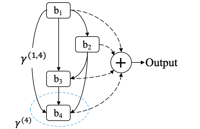
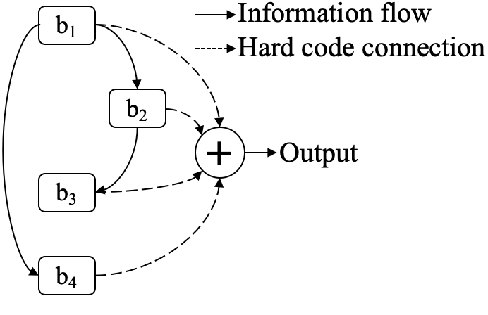
To enable heterogeneous ST-blocks, we allow the ST-blocks to have different micro architectures. This is achieved by using distinct micro architecture parameters for each ST-block. Specifically, we use architecture parameters and to parameterizing the micro search space of ST-block . The joint search space, which is composed of both the micro and macro search spaces, is parameterized by .
3.4. Search Strategy
The goal of the architecture search is to learn the architecture parameter by training the macro-DAG, governed by , and multiple heterogeneous micro-DAGs governed by , in an end-to-end manner. We design a search strategy to achieve this.
The learning of AutoCTS follows a two-stage strategy—(i) architecture search and (ii) architecture evaluation. In the architecture search stage, we run AutoCTS on the training set to search for an optimal ST-backbone. To do this, we first divide the training data evenly into a pseudo-training data and a pseudo-validation data , which are used to train both the architecture parameters and the network weights , e.g., kernels in CNNs and GCNs, projection matrices in Attentions. Specifically, we adopt a bi-level optimization algorithm to optimize and .
| (19) |
| (20) |
where and denote the losses (e.g., mean absolute error or mean squared error) on the pseudo-training and pseudo-validation data, respectively. We employ first-order approximation to speed-up the architecture search (Liu et al., 2018b). The detailed training process is shown in Algorithm 1, where and are the learning rates for the two optimizers for and , respectively.
Input: Correlated time series , Adjacency matrix ;
In the architecture evaluation stage, we only keep the architecture parameters but discard the learned network weights from the architecture search stage. This means that we only keep the learned neural architecture of the learned ST-backbone. Instead, we train the forecasting model with the learned ST-backbone from scratch on the original training and validation sets to obtain new network weights . Finally, we report the accuracy of the forecasting model with on the testing set.
4. Experiments
We evaluate AutoCTS on both single- and multi-step time series forecasting tasks using eight correlated time series datasets from different domains to justify our design choices.
4.1. Experimental Settings
4.1.1. Datasets
To enable fair comparisons with existing studies and to facilitate reproducibility, we employ eight commonly used benchmark datasets for correlated time series forecasting, including six datasets for multi-step forecasting (Yu et al., 2018; Guo et al., 2019; Li et al., 2018; Wu et al., 2019; Bai et al., 2020; Song et al., 2020) and two datasets for single-step forecasting (Lai et al., 2018; Shih et al., 2019).
Multi-step forecasting:
-
•
METR-LA and PEMS-BAY: Both datasets are traffic speed time series datasets, released by Li et al. (Li et al., 2018). The two datasets are collected from highways in the Los Angeles County and the Bay area, respectively.
-
•
PEMS03, PEMS04, PEMS07 and PEMS08: All datasets are traffic flow time series collected from the Caltrans Performance Measurement System (PeMS), which are released by Song et al. (Song et al., 2020).
Table 4 summarizes the statistics of the six datasets. This includes , the number of time seriesor nodes, and , the total number of timestamps. We adopt the same train-validation-test splits as in the original papers (Li et al., 2018; Song et al., 2020), as shown in the “Split Ratio” column in Table 4. All the time series in the six dataset have a record every 5 minutes, and thus there are 12 records per hour. Following existing literature (Li et al., 2018; Wu et al., 2019, 2020), we consider a multi-step forecasting setting where we use the recent one hour in the history (i.e., input=12 timestamps) to forecast the records in the next hour (i.e., output=12 timestamps). For each dataset, a graph is constructed where each node represents a sensor that generates a time series. The adjacency matrix represents the road network distances among the sensors (Yu et al., 2018; Li et al., 2018; Wu et al., 2019; Song et al., 2020).
| Dataset | Split Ratio | Input | Output | ||
|---|---|---|---|---|---|
| METR-LA | 207 | 34,272 | 7:1:2 | 12 | 12 |
| PEMS-BAY | 325 | 52,116 | 7:1:2 | 12 | 12 |
| PEMS03 | 358 | 26,208 | 6:2:2 | 12 | 12 |
| PEMS04 | 307 | 16,992 | 6:2:2 | 12 | 12 |
| PEMS07 | 883 | 28,224 | 6:2:2 | 12 | 12 |
| PEMS08 | 170 | 17,856 | 6:2:2 | 12 | 12 |
| Solar-energy | 137 | 52,560 | 6:2:2 | 168 | 1 |
| Electricity | 321 | 26,304 | 6:2:2 | 168 | 1 |
To enable direct and fair comparisons with existing studies (Li et al., 2018; Wu et al., 2019, 2020; Song et al., 2020; Bai et al., 2020), for METR-LA and PEMS-BAY, we report accuracy of the forecasts on the 3rd, 6th, and 12th timestamps, corresponding to the next 15-min, 30-min, and 60-min, respectively; for PEMS03, PEMS04, PEMS07, and PEMS08, we report the average accuracy over all 12 future timestamps.
Single-step forecasting:
-
•
Solar-Energy: The solar power production records collected from 137 PV plants in the Alabama State, released by Lai et al. (Lai et al., 2018)
-
•
Electricity: The electricity consumption records collected from 321 clients, released by Lai et al. (Lai et al., 2018).
The statistics of the two datasets are also summarized in Table 4. We also use the same train-validation-test splits as the original paper (Lai et al., 2018). Similar to the multi-step forecasting, we consider a well-known single-step forecasting setup to enable fair comparions with existing studies. Specifically, we use the historical 168 timestamps (i.e., input=168 timestamps) to predict the value in a single future timestamp (i.e., output=1 timestamp). The single future timestamp is either 3 or 24. There is no predefined adjacency matrix for Solar-Energy and Electricity datasets.
4.1.2. Evaluation Metrics
Following the evaluation methodology in previous studies (Li et al., 2018; Wu et al., 2019; Lai et al., 2018; Wu et al., 2020), we use mean absolute error (MAE), root mean squared error (RMSE), mean absolute percentage error (MAPE) to evaluate the accuracy of multi-step forecasting, and use Root Relative Squared Error (RRSE) and Empirical Correlation Coefficient (CORR) to measure the accuracy of single-step forecasting. For MAE, RMSE, MAPE, and RRSE, lower values indicate higher accuracy, while larger CORR values indicate higher accuracy.
4.1.3. Baselines
We compare AutoCTS with eight methods, including seven methods that are manually designed by human experts and one automated approach. The implementations of the baselines are based on the public-available code released by their authors.
-
•
DCRNN: Diffusion convolutional recurrent neural network uses diffusion GCN with GRU to build ST-blocks, and employs an encoder-decoder architecture for multi-step forecasting (Li et al., 2018).
-
STGCN: Spatio-temporal graph convolutional network adopts a Chebyshev GCN and a gated 1D convolution to build ST-blocks (Yu et al., 2018).
-
Graph WaveNet: It employs diffusion GCN and GDCC to build ST-blocks (Wu et al., 2019).
-
AGCRN: Adaptive graph convolutional recurrent network combines enhanced Chebyshev GCN and GRU to build ST-blocks (Bai et al., 2020).
-
LSTNet: A long- and short-term time-series network, which combines 1D convolution and GRU to extract short-term and long-term temporal dependencies (Lai et al., 2018).
-
TPA-LSTM: An attention based recurrent neural network (Shih et al., 2019).
-
MTGNN: A multivariate time series forecasting model with graph neural networks, which utilizes a spatial-based GCN and GDCC to construct ST-blocks (Wu et al., 2020).
-
AutoSTG: A NAS based method for automated spatio-temporal graph prediction, which uses only diffusion GCN and 1D convolution as the S/T operators in the search space for only ST-blocks but not ST-backbones, and employs meta learning to learn the weights for the diffusion GCN and 1D convolution (Pan et al., 2021).
4.1.4. Implementation Details
All the model training experiments are conducted on Nvidia Quadro RTX 8000 GPUs. The source code is available at %leave␣empty␣if␣no␣availability␣url␣should␣be␣sethttps://github.com/WXL520/AutoCTS.
Architecture Search. Following Liu et al. (Liu et al., 2018b), we use the ReLU-operator-BN order for all parametric operators to improve the training stability. We vary the number of nodes in the micro-DAG among 3, 5, and 7, and vary the number of nodes in the macro-DAG among 2, 4, 6, with default values shown in bold, for all datasets. We adopt Adam (Kingma and Ba, 2014) as the optimizer for both the architecture parameters and the network weights . For , we set the initial learning rate to , the momentum to , and the weight decay to . For , we set the initial learning rate to , and the weight decay to . We adopt partial channels (Xu et al., 2019) to improve the memory efficiency, where we select features during training. For all datasets, we set the initial temperature to and use exponential annealing with a multiplicative factor of to gradually reduce it as training evolves until it reaches .
4.2. Experimental Results
| Data | Models | 15 min | 30 min | 60 min | ||||||
|---|---|---|---|---|---|---|---|---|---|---|
| MAE | RMSE | MAPE | MAE | RMSE | MAPE | MAE | RMSE | MAPE | ||
| METR-LA | DCRNN | 2.77 | 5.38 | 7.30% | 3.15 | 6.45 | 8.80% | 3.60 | 7.60 | 10.50% |
| STGCN | 2.88 | 5.74 | 7.62% | 3.47 | 7.24 | 9.57% | 4.59 | 9.40 | 12.70% | |
| Graph WaveNet | 2.69 | 5.15 | 6.90% | 3.07 | 6.22 | 8.37% | 3.53 | 7.37 | 10.01% | |
| AGCRN | 2.83 | 5.45 | 7.56% | 3.20 | 6.55 | 8.79% | 3.58 | 7.41 | 10.13% | |
| MTGNN | 2.69 | 5.18 | 6.86% | 3.05 | 6.17 | 8.19% | 3.49 | 7.23 | 9.87% | |
| AutoSTG | 2.70 | 5.16 | 6.91% | 3.06 | 6.17 | 8.30% | 3.47 | 7.27 | 9.87% | |
| AutoCTS | 2.67 | 5.11 | 6.80% | 3.05 | 6.11 | 8.15% | 3.47 | 7.14 | 9.81% | |
| PEMS-BAY | DCRNN | 1.38 | 2.95 | 2.90% | 1.74 | 3.97 | 3.90% | 2.07 | 4.74 | 4.90% |
| STGCN | 1.36 | 2.96 | 2.90% | 1.81 | 4.27 | 4.17% | 2.49 | 5.69 | 5.79% | |
| Graph WaveNet | 1.30 | 2.74 | 2.73% | 1.63 | 3.70 | 3.67% | 1.95 | 4.52 | 4.63% | |
| AGCRN | 1.35 | 2.83 | 2.87% | 1.69 | 3.81 | 3.84% | 1.96 | 4.52 | 4.67% | |
| MTGNN | 1.32 | 2.79 | 2.77% | 1.65 | 3.74 | 3.69% | 1.94 | 4.49 | 4.53% | |
| AutoSTG | 1.31 | 2.76 | 2.73% | 1.63 | 3.67 | 3.63% | 1.92 | 4.38 | 4.43% | |
| AutoCTS | 1.30 | 2.71 | 2.69% | 1.61 | 3.62 | 3.55% | 1.89 | 4.32 | 4.36% | |
| Data | Metric | DCRNN | STGCN | Graph WaveNet | AGCRN | MTGNN | AutoCTS |
|---|---|---|---|---|---|---|---|
| PEMS03 | MAE | 18.18 | 17.49 | 14.82 | 15.89 | 15.10 | 14.71 |
| RMSE | 30.31 | 30.12 | 25.24 | 28.12 | 25.93 | 24.54 | |
| MAPE | 18.91% | 17.15% | 16.16% | 15.38% | 15.67% | 14.39% | |
| PEMS04 | MAE | 24.70 | 22.70 | 19.16 | 19.83 | 19.32 | 19.13 |
| RMSE | 38.12 | 35.55 | 30.46 | 32.26 | 31.57 | 30.44 | |
| MAPE | 17.12% | 14.59% | 13.26% | 12.97% | 13.52% | 12.89% | |
| PEMS07 | MAE | 25.30 | 25.38 | 21.54 | 21.31 | 22.07 | 20.93 |
| RMSE | 38.58 | 38.78 | 34.23 | 35.06 | 35.80 | 33.69 | |
| MAPE | 11.66% | 11.08% | 9.22% | 9.13% | 9.21% | 8.90% | |
| PEMS08 | MAE | 17.86 | 18.02 | 15.13 | 15.95 | 15.71 | 14.82 |
| RMSE | 27.83 | 27.83 | 24.07 | 25.22 | 24.62 | 23.64 | |
| MAPE | 11.45% | 11.40% | 10.10% | 10.09% | 10.03% | 9.51% |
| DataSet | Search | Memory |
|---|---|---|
| Time | ||
| METR-LA | 21.43 | 20,109 |
| PEMS-BAY | 52.60 | 32,117 |
| PEMS03 | 25.95 | 34,401 |
| PEMS04 | 14.64 | 30,681 |
| PEMS07 | 61.74 | 33,057 |
| PEMS08 | 12.34 | 16,521 |
| Solar-Energy | 163.21 | 30,977 |
| Electricity | 145.68 | 36,339 |
4.2.1. Multi-step Forecasting Accuracy
Tables 5 and 7 present the overall accuracy of AutoCTS and the baselines on multi-step forecasting datasets. We use bold to highlight the best accuracy and underline the second best accuracy. Since AutoSTG relies on additional information on the road network to enable meta learning based weight generation, and such information is unavailable on the four PEMS datasets, AutoSTG is thus unable to work on the four PEMS datasets.
Key observations are as follows. First, AutoCTS outperforms all manually designed models on all multi-step forecasting tasks, demonstrating that AutoCTS is able to produce very competitive ST-blocks and ST-backbones that outperform human designed models.
Second, when comparing to the other automated approach AutoSTG, although AutoSTG includes additional features, such as GPS coordinates of sensors, to enhance its forecasting accuracy, it is still inferior to AutoCTS except for the MAE at the 60-min timestamp on METR-LA. This is due to (i) AutoSTG only include diffusion GCN and 1D convolution to construct the search space, while we follow the proposed two principles to select a compact yet complementary S/T operators. (ii) AutoSTG only searches for the micro architecture of a single ST-block, and then stacks the ST-blocks to build the forecasting model. In contrast, we jointly search for both the micro architecture of ST-blocks and the macro architecture of the ST-backbone.
Third, AutoCTS outperforms AGCRN and DCRNN, which both employ GRU to model temporal dependencies. This justifies our design choices that disregard the RNN family in the micro search space.
Fourth, there does not exist a single manually-designed model that consistently outperforms other manually-designed models. For example, MTGNN outperforms Graph WaveNet on METR-LA, but is outperformed by Graph WaveNet on PEMS04. This suggests that the optimal neural architectures for different datasets may be different, which implies that it is beneficial to be able to automatically identify forecasting models with unique architectures for different datasets, which is what AutoCTS is able to offer.
4.2.2. Single-step Forecasting Accuracy
Table 8 shows the experimental results on the two single-step forecasting datasets. We observe that: (1) AutoCTS and MTGNN outperform LSTNet and TPA-LSTM. This is because LSTNet and TPA-LSTM do not explicitly model the correlations among different time series. In contrast, both AutoCTS and MTGNN simultaneously model the temporal and spatial dependencies. AutoCTS does not outperform MTGNN much for single-step forecasting when compared to multi-step forecasting. This suggests that MTGNN is already a very effective model that behaves similarly to the optimal model identified from the search space of AutoCTS for single-step forecasting, but is less effective for multi-step forecasting. This further justifies the needs for automated solutions for identifying specific, optimal models for different forecasting tasks. (2) AutoCTS achieves the best accuracy on both short-term (see Table 5 and Table 7) and long-term (see Table 8) datasets. This is because our search space contains GDCC and INF-T, which are good at modeling both short- and long-term dependencies, respectively, which enables AutoCTS to generate high-performance models in both cases.
| Data | Solar-Energy | Electricity | |||
|---|---|---|---|---|---|
| Models | Metric | 3 | 24 | 3 | 24 |
| LSTNet | RRSE | 0.1843 | 0.4643 | 0.0864 | 0.1007 |
| CORR | 0.9843 | 0.8870 | 0.9283 | 0.9119 | |
| TPA-LSTM | RRSE | 0.1803 | 0.4389 | 0.0823 | 0.1006 |
| CORR | 0.9850 | 0.9081 | 0.9439 | 0.9133 | |
| MTGNN | RRSE | 0.1778 | 0.4270 | 0.0745 | 0.0953 |
| CORR | 0.9852 | 0.9031 | 0.9474 | 0.9234 | |
| AutoCTS | RRSE | 0.1750 | 0.4143 | 0.0743 | 0.0947 |
| CORR | 0.9855 | 0.9085 | 0.9477 | 0.9239 | |
4.2.3. Ablation Studies
We conduct ablation studies to justify the design choices used in AutoCTS.
| Models | 15 min | 30 min | 60 min | GPU hours | ||||||
|---|---|---|---|---|---|---|---|---|---|---|
| MAE | RMSE | MAPE | MAE | RMSE | MAPE | MAE | RMSE | MAPE | ||
| AutoCTS | 2.67 | 5.11 | 6.80% | 3.05 | 6.11 | 8.15% | 3.47 | 7.14 | 9.81% | 21.43 |
| w/o design principles | 2.72 | 5.20 | 6.97% | 3.12 | 6.27 | 8.42% | 3.57 | 7.34 | 9.98% | 96.79 |
| w/o temperature | 2.75 | 5.21 | 6.89% | 3.13 | 6.19 | 8.23% | 3.55 | 7.20 | 9.84% | 21.42 |
| w/o macro search | 2.68 | 5.07 | 6.76% | 3.07 | 6.09 | 8.08% | 3.56 | 7.22 | 9.75% | 21.37 |
| macro only | 2.73 | 5.21 | 7.02% | 3.07 | 6.20 | 8.34% | 3.51 | 7.29 | 10.02% | 10.97 |
| Models | 15 min | 30 min | 60 min | GPU hours | ||||||
|---|---|---|---|---|---|---|---|---|---|---|
| MAE | RMSE | MAPE | MAE | RMSE | MAPE | MAE | RMSE | MAPE | ||
| AutoCTS | 1.30 | 2.71 | 2.69% | 1.61 | 3.62 | 3.55% | 1.89 | 4.32 | 4.36% | 52.60 |
| w/o design principles | 1.30 | 2.72 | 2.71% | 1.62 | 3.64 | 3.62% | 1.92 | 4.38 | 4.52% | 223.56 |
| w/o temperature | 1.31 | 2.72 | 2.72% | 1.63 | 3.65 | 3.68% | 1.93 | 4.42 | 4.54% | 52.63 |
| w/o macro search | 1.31 | 2.74 | 2.69% | 1.62 | 3.66 | 3.55% | 1.89 | 4.35 | 4.40% | 52.31 |
| macro only | 1.34 | 2.77 | 2.83% | 1.65 | 3.68 | 3.74% | 1.95 | 4.42 | 4.66% | 24.08 |
| Models | Metrics | GPU hours | ||
|---|---|---|---|---|
| MAE | RMSE | MAPE | ||
| AutoCTS | 14.71 | 24.54 | 14.39% | 25.95 |
| w/o design principles | 15.66 | 25.51 | 15.28% | 126.25 |
| w/o temperature | 14.87 | 24.93 | 14.64% | 25.97 |
| w/o macro search | 15.07 | 25.22 | 14.84% | 25.89 |
| macro only | 15.83 | 26.12 | 15.77% | 15.90 |
| Models | Metrics | GPU hours | ||
|---|---|---|---|---|
| MAE | RMSE | MAPE | ||
| AutoCTS | 19.13 | 30.44 | 12.89% | 14.64 |
| w/o design principles | 19.33 | 30.64 | 12.98% | 48.40 |
| w/o temperature | 19.23 | 30.59 | 13.03% | 14.64 |
| w/o macro search | 19.59 | 30.86 | 13.07% | 14.60 |
| macro only | 20.14 | 31.41 | 13.97% | 8.27 |
| Models | Metrics | GPU hours | ||
|---|---|---|---|---|
| MAE | RMSE | MAPE | ||
| AutoCTS | 20.93 | 33.69 | 8.90% | 61.74 |
| w/o design principles | 21.03 | 33.78 | 9.01% | 247.67 |
| w/o temperature | 21.16 | 34.12 | 9.22% | 61.71 |
| w/o macro search | 21.23 | 34.02 | 9.20% | 61.68 |
| macro only | 22.91 | 36.02 | 10.16% | 31.64 |
| Models | Metrics | GPU hours | ||
|---|---|---|---|---|
| MAE | RMSE | MAPE | ||
| AutoCTS | 14.82 | 23.64 | 9.51% | 12.34 |
| w/o design principles | 15.48 | 24.21 | 10.33% | 46.13 |
| w/o temperature | 15.03 | 23.69 | 9.69% | 12.34 |
| w/o macro search | 15.24 | 24.17 | 9.91% | 12.32 |
| macro only | 16.03 | 24.91 | 10.92% | 6.78 |
| Models | 3 | 24 | GPU hours | ||
|---|---|---|---|---|---|
| RRSE | CORR | RRSE | CORR | ||
| AutoCTS | 0.1750 | 0.9855 | 0.4143 | 0.9085 | 163.21 |
| w/o design principles | 0.1783 | 0.9846 | 0.4159 | 0.9062 | 559.09 |
| w/o temperature | 0.1658 | 0.9875 | 0.4109 | 0.9084 | 163.37 |
| w/o macro search | 0.1763 | 0.9847 | 0.4158 | 0.9034 | 162.70 |
| macro only | 0.1787 | 0.9832 | 0.4183 | 0.9029 | 98.31 |
| Models | 3 | 24 | GPU hours | ||
|---|---|---|---|---|---|
| RRSE | CORR | RRSE | CORR | ||
| AutoCTS | 0.0743 | 0.9477 | 0.0947 | 0.9239 | 145.68 |
| w/o design principles | 0.0753 | 0.9464 | 0.0952 | 0.9227 | 494.15 |
| w/o temperature | 0.0753 | 0.9457 | 0.0958 | 0.9231 | 145.73 |
| w/o macro search | 0.0780 | 0.9441 | 0.0963 | 0.9206 | 145.62 |
| macro only | 0.0832 | 0.9230 | 0.0950 | 0.9168 | 85.19 |
| M | 15 min | 30 min | 60 min | ||||||
|---|---|---|---|---|---|---|---|---|---|
| MAE | RMSE | MAPE | MAE | RMSE | MAPE | MAE | RMSE | MAPE | |
| 3 | 2.71 | 5.14 | 6.91% | 3.08 | 6.16 | 8.41% | 3.54 | 7.26 | 10.08% |
| 5 | 2.67 | 5.11 | 6.80% | 3.05 | 6.11 | 8.15% | 3.47 | 7.14 | 9.81% |
| 7 | 2.73 | 5.22 | 7.07% | 3.11 | 6.25 | 8.38% | 3.56 | 7.37 | 10.21% |
| B | 15 min | 30 min | 60 min | ||||||
|---|---|---|---|---|---|---|---|---|---|
| MAE | RMSE | MAPE | MAE | RMSE | MAPE | MAE | RMSE | MAPE | |
| 2 | 2.70 | 5.11 | 6.96% | 3.07 | 6.07 | 8.42% | 3.50 | 7.09 | 10.15% |
| 4 | 2.67 | 5.11 | 6.80% | 3.05 | 6.11 | 8.15% | 3.47 | 7.14 | 9.81% |
| 6 | 2.68 | 5.09 | 6.88% | 3.04 | 6.07 | 8.35% | 3.50 | 7.18 | 10.18% |
| M | 15 min | 30 min | 60 min | ||||||
|---|---|---|---|---|---|---|---|---|---|
| MAE | RMSE | MAPE | MAE | RMSE | MAPE | MAE | RMSE | MAPE | |
| 3 | 1.30 | 2.70 | 2.71% | 1.62 | 3.65 | 3.65% | 1.91 | 4.38 | 4.55% |
| 5 | 1.30 | 2.71 | 2.69% | 1.61 | 3.62 | 3.55% | 1.89 | 4.32 | 4.36% |
| 7 | 1.32 | 2.73 | 2.76% | 1.64 | 3.72 | 3.69% | 1.92 | 4.48 | 4.60% |
| B | 15 min | 30 min | 60 min | ||||||
|---|---|---|---|---|---|---|---|---|---|
| MAE | RMSE | MAPE | MAE | RMSE | MAPE | MAE | RMSE | MAPE | |
| 2 | 1.31 | 2.72 | 2.72% | 1.62 | 3.62 | 3.60% | 1.90 | 4.34 | 4.42% |
| 4 | 1.30 | 2.71 | 2.69% | 1.61 | 3.62 | 3.55% | 1.89 | 4.32 | 4.36% |
| 6 | 1.30 | 2.74 | 2.72% | 1.63 | 3.71 | 3.67% | 1.92 | 4.45 | 4.59% |
| M | MAE | RMSE | MAPE | B | MAE | RMSE | MAPE |
|---|---|---|---|---|---|---|---|
| 3 | 14.95 | 25.36 | 15.18% | 2 | 14.92 | 25.11 | 15.03% |
| 5 | 14.71 | 24.54 | 14.39% | 4 | 14.71 | 24.54 | 14.39% |
| 7 | 14.82 | 25.23 | 14.51% | 6 | 14.80 | 24.73 | 14.45% |
| M | MAE | RMSE | MAPE | B | MAE | RMSE | MAPE |
|---|---|---|---|---|---|---|---|
| 3 | 19.40 | 30.64 | 13.76% | 2 | 19.39 | 30.74 | 13.67% |
| 5 | 19.13 | 30.44 | 12.89% | 4 | 19.13 | 30.44 | 12.89% |
| 7 | 19.32 | 30.69 | 13.18% | 6 | 19.11 | 30.53 | 12.90% |
| M | MAE | RMSE | MAPE | B | MAE | RMSE | MAPE |
|---|---|---|---|---|---|---|---|
| 3 | 21.73 | 34.66 | 9.25% | 2 | 21.11 | 33.74 | 9.53% |
| 5 | 20.93 | 33.69 | 8.90% | 4 | 20.93 | 33.69 | 8.90% |
| 7 | 21.32 | 34.14 | 9.17% | 6 | 20.62 | 33.30 | 9.33% |
| M | MAE | RMSE | MAPE | B | MAE | RMSE | MAPE |
|---|---|---|---|---|---|---|---|
| 3 | 15.27 | 24.06 | 10.14% | 2 | 15.37 | 24.14 | 9.74% |
| 5 | 14.82 | 23.64 | 9.51% | 4 | 14.82 | 23.64 | 9.51% |
| 7 | 14.97 | 24.11 | 9.62% | 6 | 15.12 | 23.89 | 9.77% |
| M | 3 | 24 | B | 3 | 24 | ||||
|---|---|---|---|---|---|---|---|---|---|
| RRSE | CORR | RRSE | CORR | RRSE | CORR | RRSE | CORR | ||
| 3 | 0.1786 | 0.9848 | 0.4150 | 0.9062 | 2 | 0.1755 | 0.9846 | 0.4164 | 0.9040 |
| 5 | 0.1750 | 0.9855 | 0.4143 | 0.9085 | 4 | 0.1750 | 0.9855 | 0.4143 | 0.9085 |
| 7 | 0.1761 | 0.9849 | 0.4136 | 0.9073 | 6 | 0.1692 | 0.9869 | 0.4117 | 0.9089 |
| M | 3 | 24 | B | 3 | 24 | ||||
|---|---|---|---|---|---|---|---|---|---|
| RRSE | CORR | RRSE | CORR | RRSE | CORR | RRSE | CORR | ||
| 3 | 0.0752 | 0.9441 | 0.0942 | 0.9223 | 2 | 0.0749 | 0.9438 | 0.0971 | 0.9235 |
| 5 | 0.0743 | 0.9477 | 0.0947 | 0.9239 | 4 | 0.0743 | 0.9477 | 0.0947 | 0.9239 |
| 7 | 0.0755 | 0.9463 | 0.0949 | 0.9231 | 6 | 0.0748 | 0.9432 | 0.0958 | 0.9227 |
| Models | Training | Inference | Parameters |
|---|---|---|---|
| (s/epoch) | (ms/window) | ||
| DCRNN | 304.2 | 8.58 | 372,353 |
| STGCN | 16.8 | 7.32 | 119,176 |
| Graph WaveNet | 46.7 | 0.17 | 309,400 |
| AGCRN | 47.6 | 0.59 | 751,650 |
| MTGNN | 39.6 | 0.43 | 405,452 |
| AutoSTG | 453.3 | 1.60 | 509,048 |
| AutoCTS | 138.9 | 0.34 | 358,520 |
| Models | Training | Inference | Parameters |
|---|---|---|---|
| (s/epoch) | (ms/window) | ||
| DCRNN | 779.0 | 11.88 | 372,353 |
| STGCN | 41.8 | 7.24 | 119,648 |
| Graph WaveNet | 117.9 | 0.17 | 311,760 |
| AGCRN | 95.3 | 0.80 | 752,830 |
| MTGNN | 87.5 | 0.68 | 573,484 |
| AutoSTG | 613.2 | 1.97 | 553,932 |
| AutoCTS | 310.4 | 0.35 | 395,984 |
| Models | Training | Inference | Parameters |
|---|---|---|---|
| (s/epoch) | (ms/window) | ||
| DCRNN | 335.7 | 10.90 | 371,393 |
| STGCN | 18.8 | 7.18 | 119,204 |
| Graph WaveNet | 52.8 | 0.16 | 312,388 |
| AGCRN | 45.7 | 0.94 | 749,320 |
| MTGNN | 45.1 | 0.74 | 619,228 |
| AutoCTS | 149.3 | 0.34 | 351,108 |
| Models | Training | Inference | Parameters |
|---|---|---|---|
| (s/epoch) | (ms/window) | ||
| DCRNN | 226.1 | 11.69 | 371,393 |
| STGCN | 10.5 | 7.45 | 119,000 |
| Graph WaveNet | 28.5 | 0.17 | 311,368 |
| AGCRN | 21.9 | 0.74 | 748,810 |
| MTGNN | 23.6 | 0.64 | 546,604 |
| AutoCTS | 80.3 | 0.34 | 367,048 |
| Models | Training | Inference | Parameters |
|---|---|---|---|
| (s/epoch) | (ms/window) | ||
| DCRNN | 870.9 | 25.45 | 371,393 |
| STGCN | 52.8 | 13.18 | 121,304 |
| Graph WaveNet | 155.8 | 0.17 | 322,888 |
| AGCRN | 144.8 | 2.76 | 754,570 |
| MTGNN | 107.6 | 1.95 | 1,366,828 |
| AutoCTS | 381.2 | 0.35 | 407,112 |
| Models | Training | Inference | Parameters |
|---|---|---|---|
| (s/epoch) | (ms/window) | ||
| DCRNN | 157.7 | 7.61 | 371,393 |
| STGCN | 6.4 | 4.50 | 118,452 |
| Graph WaveNet | 18.7 | 0.16 | 308,628 |
| AGCRN | 16.6 | 0.53 | 150,112 |
| MTGNN | 14.1 | 0.35 | 351,516 |
| AutoCTS | 50.3 | 0.34 | 357,236 |
| Models | Training | Inference | Parameters |
|---|---|---|---|
| (s/epoch) | (ms/window) | ||
| LSTNet | 29.2 | 0.06 | 174,807 |
| TPA-LSTM | 206.8 | 11.78 | 122,295 |
| MTGNN | 218.3 | 1.82 | 347,665 |
| AutoCTS | 746.1 | 1.06 | 318,277 |
| Models | Training | Inference | Parameters |
|---|---|---|---|
| (s/epoch) | (ms/window) | ||
| LSTNet | 12.1 | 0.05 | 325,871 |
| TPA-LSTM | 252.2 | 30.94 | 193,135 |
| MTGNN | 258.9 | 4.51 | 362,385 |
| AutoCTS | 856.0 | 3.50 | 321,957 |
| Data | Models | 15 min | 30 min | 60 min | ||||||
|---|---|---|---|---|---|---|---|---|---|---|
| MAE | RMSE | MAPE | MAE | RMSE | MAPE | MAE | RMSE | MAPE | ||
| METR-LA | Transferred Model | 2.72 | 5.11 | 6.90% | 3.08 | 6.09 | 8.28% | 3.50 | 7.12 | 10.02% |
| AutoCTS | 2.67 | 5.11 | 6.80% | 3.05 | 6.11 | 8.15% | 3.47 | 7.14 | 9.81% | |
| PEMS-BAY | Transferred Model | 1.30 | 2.73 | 2.73% | 1.62 | 3.63 | 3.63% | 1.90 | 4.35 | 4.51% |
| AutoCTS | 1.30 | 2.71 | 2.69% | 1.61 | 3.62 | 3.55% | 1.89 | 4.32 | 4.36% | |
| # Edges | 15 min | 30 min | 60 min | Training (s/epoch) | ||||||
|---|---|---|---|---|---|---|---|---|---|---|
| MAE | RMSE | MAPE | MAE | RMSE | MAPE | MAE | RMSE | MAPE | ||
| 2 | 2.67 | 5.11 | 6.80% | 3.05 | 6.11 | 8.15% | 3.47 | 7.14 | 9.81% | 138.9 |
| 3 | 2.68 | 5.09 | 6.86% | 3.05 | 6.07 | 8.16% | 3.50 | 7.18 | 9.75% | 188.6 |
| # Edges | MAE | RMSE | MAPE | Training (s/epoch) |
|---|---|---|---|---|
| 2 | 14.71 | 24.54 | 14.39% | 149.3 |
| 3 | 14.58 | 24.20 | 15.40% | 204.0 |
| CNN | RNN | Attention | |
|---|---|---|---|
| GCN | (Yu et al., 2018; Guo et al., 2019; Wu et al., 2019; Huang et al., 2020; Diao et al., 2019; Fang et al., 2019; Wu et al., 2020) | (Li et al., 2018; Bai et al., 2020; Chen et al., 2020; Hu et al., 2020) | (Guo et al., 2019) |
| Attention | (Guo et al., 2019) | None | (Zheng et al., 2020; Xu et al., 2020) |
In particular, we compare AutoCTS with the following variants: (1) w/o design principles: this variant does not follow the proposed two principles for selecting a compact set of S/T operators. Rather, it includes all operators in Table 1. (2) w/o temperature: it does not use the temperature parameter to reduce the gap between the micro-DAG and the derived ST-block. (3) w/o macro search: this variant only searches for a single optimal ST-block and then sequentially stacks ST-blocks with residual connections to build an ST-backbone. (4) macro only: it employs four existing human designed ST-blocks as the atomic search units and only searches for novel ST-backbones. The selected ST-blocks come from STGCN (Yu et al., 2018), DCRNN (Li et al., 2018), Graph WaveNet (Wu et al., 2019), and MTGNN (Wu et al., 2020). We consider (1) the accuracy of the models that are identified by the different variants, and (2) the runtime in GPU hours that it takes to identify the models.
Tables 9 to 16 show that: (1) AutoCTS achieves better accuracy than its variant w/o design principles, and costs much less GPU hours for architecture search. This demonstrates the effectiveness of the proposed principles for selecting a compact and complementary S/T operators from Table 1. (2) The proposed temperature parameter helps reduce the gap and find more accurate models with similar GPU hours, except in the case of only one dataset, Solar-Energy. (3) Disabling the macro search and search for the stacking of homogeneous ST-backbone lowers the performance without significantly decreasing the searching time – the only exception is the METR-LA dataset, where the accuracies when using and no using the macro search are similar. This suggests our joint search space and strategy is effective and efficient. (4) AutoCTS significantly outperforms the macro only variant, which justifying that S/T operators are more suitable to be used as the atomic search units in the search space than manually-designed ST-blocks. Although the macro only variant is very efficient, due to its small search space, it is unappealing as many human designed models, such as Graph WaveNet, AGCRN, and MTGNN, outperform it.
4.2.4. Parameter Sensitivity Analysis
We proceed to evaluate the impact of key hyperparameters in AutoCTS, including , i.e., the number of nodes in an ST-block in the micro search space, and , i.e., the number of ST-blocks in the macro search space, and , i.e., the number of incoming edges per node in the derived ST-block. We use , , and as default values. We then vary among {3, 5, 7}, vary among {2, 4, 6}, and vary among {2, 3}, while keeping the rest to their default values.
Tables 17 to 26 show that AutoCTS achieves the best accuracy under and , except on PEMS07 and Solar-Energy, where the results are not optimal but are still comparable to the best setting. Decreasing or reduces the expressiveness of AutoCTS and thus the accuracy of the automatically identified models. A larger or increases the complexity of the micro and macro search space, resulting in potentially more overfitting problems when the training data is not abundant. Thus, it slightly degrades the accuracy. In addition, larger or may lead to models that use significantly more parameters than the baseline models.
Tables 36 and 37 show minimal accuracy improvements when increases from 2 to 3, while the training time (s/epoch) shows a clear increase. This suggests that using 2 edges per node yields sufficiently complex internal topologies for ST-blocks and avoids introducing too many parameters and thus maintaining good efficiency.
4.2.5. Case Study
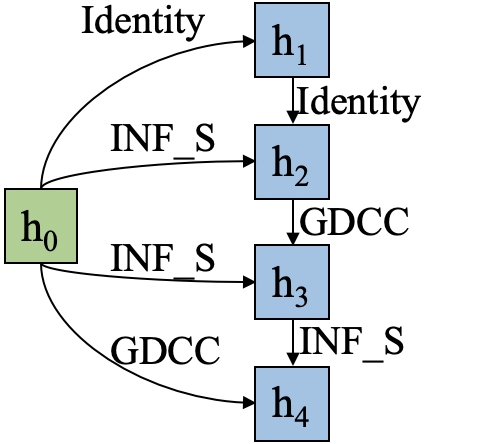
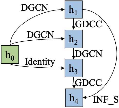
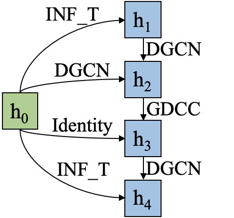
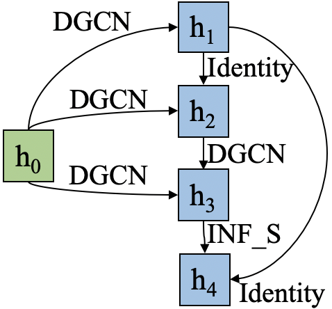
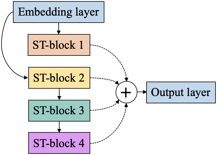
We show the architecture of the forecasting model on PEMS03 in Figure 8. As Figures 8(a), 8(b), 8(c) and 8(d) show, each ST-block has a distinct internal architecture. In particular, the four ST-blocks contain all S/T operators in the micro search space, including 5 GDCC, 2 INF-T, 5 INF-S and 10 DGCN. This indicates the effectiveness of the proposed micro search space. The ST-backbone consists of the four heterogeneous ST-blocks, which are assembled by diverse topologies. This justifies the needs of enabling topologically flexible, heterogeneous ST-backbone, which most existing models fail to support.
4.2.6. Transferability
Since manually designed forecasting models are often applied to different datasets, it is pertinent to investigate the transferability of forecasting models learned by AutoCTS to assess how such models compare with traditional, manually designed models. To this end, we consider a “Transferred Model” that is identified automatically by AutoCTS on the PEMS03 dataset, as shown in Figure 8. We apply this model to make forecasts on datasets METR-LA and PEMS-BAY. The results are shown in Table 35, where AutoCTS denotes the automatically identified model on METR-LA or PEMS-BAY. The transferred model achieves competitive accuracy on METR-LA and PEMS-BAY. Although the transferred model is not as good as the model that is directly learned by AutoCTS on the specific dataset, it is able to outperform the baselines on most metrics, especially in the case of PEMS-BAY (cf. Table 5). This is evidence that AutoCTS is able to produce effective and transferable forecasting models.
4.2.7. Runtime, Memory Costs & Number of Parameters
For the architecture search phase, we consider the runtime and memory that AutoCTS takes. Table 7 shows that the search time varies from 12.34 to 163.21 GPU hours across datasets, depending on the number of time series/nodes, the total number of timestamps, and the length of the input time window. The searching process takes up to ca. 36 GB memory, which can fit into the memory of a single modern GPU.
To understand how models identified by AutoCTS and baseline models compare in terms of time and space, we report the training time (seconds per epoch), inference time (milliseconds per window), and total number of parameters in Tables 28 to 34. First, in terms of training time, AutoCTS is faster than DCRNN and AutoSTG but slower than other models. It’s because AutoCTS includes operators from both the CNN and Attention families, where Attention operators are less efficient than CNN operators. Besides, AutoCTS is much deeper than DCRNN and AGCRN. DCRNN and AutoSTG are slow because the former sequentially produces predictions at all time steps, and the latter employs meta-learning to learn the network weights.
Second, in terms of inference time, all methods are able to make near-instantaneous predictions when new data arrives and are thus able to support online prediction in streaming settings. Third, in terms of the number of parameters, AutoCTS often uses fewer parameters than do MTGNN, AGCRN, and AutoSTG, uses more parameters than does STGCN (whose accuracy is among the worst), and is comparable to the other methods.
5. Related work
We categorize existing studies on CTS forecasting into two categories—manually designed models vs. automated designed models.
Manually Designed Models. Recent deep learning models achieve the state-of-the-art accuracy in correlated time series forecasting. Such models rely on different types of human designed ST-blocks that capture both temporal dependencies and spatial correlations. Table 38 summarizes the ST-blocks in the literature according to two dimensions—temporal dependencies modeling (including the CNN, RNN and attention families) vs. spatial correlation modeling (including the GCN and attention families).
Automatically Designed Models. Neural Architecture Search (NAS) has been employed to automatically design neural architectures for the many tasks. Existing NAS methods can be divided into evolutionary algorithm based (So et al., 2019), reinforcement learning based (Pham et al., 2018), performance predictor based (Li et al., 2020a) and gradient-based methods (Liu et al., 2018b). AutoCTS is a gradient-based method due to its high efficiency. Despite of great success in computer vision (Pham et al., 2018; Chen et al., 2018), natural language processing (So et al., 2019), and AutoML systems (Zogaj et al., 2021; Li et al., 2021), little effort has been devoted to time series forecasting.
AutoST (Li et al., 2020b) is proposed for spatio-temporal prediction, where the time series are from a uniform grid. The values at each timestamp are considered as an image, and then a search space that only contains convolution operators is proposed. AutoST does not apply in our setting, where time series are not necessarily from a uniform grid, making the image modeling inapplicable. AutoSTG (Pan et al., 2021) considers correlated time series forecasting. However, it differs from AutoCTS in the following perspective. (1) AutoSTG only considers one T-operator and one S-operator, i.e., 1D convolution and Diffusion GCN. In contrast, we propose two principles to select the most effective and efficient operators from diverse families. (2) AutoSTG only designs ST-blocks, whereas we search jointly both ST-blocks and the ST-backbone. (3) AutoSTG relies on additional information of the graph to enable meta-learning to learn network weight . In contrast, AutoCTS does not rely on such additional information but purely on the time series themselves. Thus, AutoCTS has a wider application scope.
6. Conclusion
We present AutoCTS, a framework that is able to automatically learn a neural network model for correlated time series forecasting. In particular, we design a micro search space with a compact set of S/T operators to find novel ST-blocks. In addition, we design a macro search space to identify the topology among heterogeneous ST-blocks to construct novel ST-backbones. Extensive experiments on eight commonly used correlated time series forecasting datasets justify the design choices of AutoCTS. As future work, it is of interest to include model efficiency as an additional criterion into the search strategy to automatically identify both accurate and efficient models and to employ parallel computing techniques (Yuan et al., 2010) to make the search more efficient. It is also of interest to extend AutoCTS to other analytics tasks, such as outlier detection (Kieu et al., 2022) and trajectory analytics (Yang et al., 2021).
Acknowledgements.
This work was partially supported by Independent Research Fund Denmark under agreements 8022-00246B and 8048-00038B, the VILLUM FONDEN under agreements 34328 and 40567, and the Innovation Fund Denmark centre, DIREC.References
- (1)
- Bai et al. (2020) Lei Bai, Lina Yao, Can Li, Xianzhi Wang, and Can Wang. 2020. Adaptive Graph Convolutional Recurrent Network for Traffic Forecasting. In NeurIPS, Vol. 33. 17804–17815.
- Campos et al. (2022) David Campos, Tung Kieu, Chenjuan Guo, Feiteng Huang, Kai Zheng, Bin Yang, and Christian S. Jensen. 2022. Unsupervised Time Series Outlier Detection with Diversity-Driven Convolutional Ensembles. Proc. VLDB Endow. 15, 3 (2022), 611–623.
- Chen et al. (2018) Liang-Chieh Chen, Maxwell D Collins, Yukun Zhu, George Papandreou, Barret Zoph, Florian Schroff, Hartwig Adam, and Jonathon Shlens. 2018. Searching for efficient multi-scale architectures for dense image prediction. In NeurIPS. 8713–8724.
- Chen et al. (2020) Weiqi Chen, Ling Chen, Yu Xie, Wei Cao, Yusong Gao, and Xiaojie Feng. 2020. Multi-range attentive bicomponent graph convolutional network for traffic forecasting. In AAAI, Vol. 34. 3529–3536.
- Cirstea et al. (2018) Razvan-Gabriel Cirstea, Darius-Valer Micu, Gabriel-Marcel Muresan, Chenjuan Guo, and Bin Yang. 2018. Correlated Time Series Forecasting using Multi-Task Deep Neural Networks. In CIKM. 1527–1530.
- Cirstea et al. (2021) Razvan-Gabriel Cirstea, Tung Kieu, Chenjuan Guo, Bin Yang, and Sinno Jialin Pan. 2021. EnhanceNet: Plugin Neural Networks for Enhancing Correlated Time Series Forecasting. In ICDE. 1739–1750.
- Cirstea et al. (2019) Razvan-Gabriel Cirstea, Bin Yang, and Chenjuan Guo. 2019. Graph Attention Recurrent Neural Networks for Correlated Time Series Forecasting. In MileTS19@KDD.
- Dauphin et al. (2017) Yann N Dauphin, Angela Fan, Michael Auli, and David Grangier. 2017. Language modeling with gated convolutional networks. In ICML. 933–941.
- Diao et al. (2019) Zulong Diao, Xin Wang, Dafang Zhang, Yingru Liu, Kun Xie, and Shaoyao He. 2019. Dynamic spatial-temporal graph convolutional neural networks for traffic forecasting. In AAAI, Vol. 33. 890–897.
- Elsken et al. (2019) Thomas Elsken, Jan Hendrik Metzen, and Frank Hutter. 2019. Neural Architecture Search: A Survey. Journal of Machine Learning Research 20 (2019), 1–21.
- Fang et al. (2019) Shen Fang, Qi Zhang, Gaofeng Meng, Shiming Xiang, and Chunhong Pan. 2019. GSTNet: Global Spatial-Temporal Network for Traffic Flow Prediction. In IJCAI. 2286–2293.
- Gehring et al. (2017) Jonas Gehring, Michael Auli, David Grangier, Denis Yarats, and Yann N Dauphin. 2017. Convolutional sequence to sequence learning. In ICML. 1243–1252.
- Guo et al. (2020) Chenjuan Guo, Bin Yang, Jilin Hu, Christian S. Jensen, and Lu Chen. 2020. Context-aware, preference-based vehicle routing. Proc. VLDB Endow. 29, 5 (2020), 1149–1170.
- Guo et al. (2019) Shengnan Guo, Youfang Lin, Ning Feng, Chao Song, and Huaiyu Wan. 2019. Attention based spatial-temporal graph convolutional networks for traffic flow forecasting. In AAAI, Vol. 33. 922–929.
- Hu et al. (2018) Jilin Hu, Bin Yang, Chenjuan Guo, and Christian S. Jensen. 2018. Risk-aware path selection with time-varying, uncertain travel costs: a time series approach. Proc. VLDB Endow. 27, 2 (2018), 179–200.
- Hu et al. (2020) Jilin Hu, Bin Yang, Chenjuan Guo, Christian S. Jensen, and Hui Xiong. 2020. Stochastic Origin-Destination Matrix Forecasting Using Dual-Stage Graph Convolutional, Recurrent Neural Networks. In ICDE. 1417–1428.
- Huang et al. (2020) Rongzhou Huang, Chuyin Huang, Yubao Liu, Genan Dai, and Weiyang Kong. 2020. LSGCN: Long Short-Term Traffic Prediction with Graph Convolutional Networks. In IJCAI. 2355–2361.
- Kalchbrenner et al. (2016) Nal Kalchbrenner, Lasse Espeholt, Karen Simonyan, Aaron van den Oord, Alex Graves, and Koray Kavukcuoglu. 2016. Neural machine translation in linear time. arXiv preprint arXiv:1610.10099 (2016).
- Khandelwal et al. (2018) Urvashi Khandelwal, He He, Peng Qi, and Dan Jurafsky. 2018. Sharp Nearby, Fuzzy Far Away: How Neural Language Models Use Context. In ACL. 284–294.
- Kieu et al. (2022) Tung Kieu, Bin Yang, Chenjuan Guo, Razvan-Gabriel Cirstea, Yan Zhao, Yale Song, and Christian S. Jensen. 2022. Anomaly Detection in Time Series with Robust Variational Quasi-Recurrent Autoencoders.. In ICDE.
- Kieu et al. (2018) Tung Kieu, Bin Yang, Chenjuan Guo, and Christian S. Jensen. 2018. Distinguishing Trajectories from Different Drivers using Incompletely Labeled Trajectories. In CIKM. 863–872.
- Kingma and Ba (2014) Diederik P Kingma and Jimmy Ba. 2014. Adam: A method for stochastic optimization. arXiv preprint arXiv:1412.6980 (2014).
- Kipf and Welling (2017) Thomas N. Kipf and Max Welling. 2017. Semi-Supervised Classification with Graph Convolutional Networks. In ICLR.
- Lai et al. (2018) Guokun Lai, Wei-Cheng Chang, Yiming Yang, and Hanxiao Liu. 2018. Modeling long-and short-term temporal patterns with deep neural networks. In SIGIR. 95–104.
- Li and Zhu (2021) Mengzhang Li and Zhanxing Zhu. 2021. Spatial-Temporal Fusion Graph Neural Networks for Traffic Flow Forecasting. In AAAI, Vol. 35. 4189–4196.
- Li et al. (2020b) Ting Li, Junbo Zhang, Kainan Bao, Yuxuan Liang, Yexin Li, and Yu Zheng. 2020b. Autost: Efficient neural architecture search for spatio-temporal prediction. In SIGKDD. 794–802.
- Li et al. (2020a) Wei Li, Shaogang Gong, and Xiatian Zhu. 2020a. Neural graph embedding for neural architecture search. In AAAI, Vol. 34. 4707–4714.
- Li et al. (2021) Yang Li, Yu Shen, Wentao Zhang, Jiawei Jiang, Bolin Ding, Yaliang Li, Jingren Zhou, Zhi Yang, Wentao Wu, Ce Zhang, et al. 2021. VolcanoML: speeding up end-to-end AutoML via scalable search space decomposition. Proc. VLDB Endow. 14 (2021), 2167–2176.
- Li et al. (2018) Yaguang Li, Rose Yu, Cyrus Shahabi, and Yan Liu. 2018. Diffusion Convolutional Recurrent Neural Network: Data-Driven Traffic Forecasting. In ICLR.
- Liu et al. (2018a) Huiping Liu, Cheqing Jin, Bin Yang, and Aoying Zhou. 2018a. Finding Top-k Optimal Sequenced Routes. In ICDE. 569–580.
- Liu et al. (2018b) Hanxiao Liu, Karen Simonyan, and Yiming Yang. 2018b. DARTS: Differentiable Architecture Search. In ICLR.
- Mei et al. (2019) Jieru Mei, Yingwei Li, Xiaochen Lian, Xiaojie Jin, Linjie Yang, Alan Yuille, and Jianchao Yang. 2019. AtomNAS: Fine-Grained End-to-End Neural Architecture Search. In ICLR.
- Oord et al. (2016) Aäron van den Oord, Nal Kalchbrenner, Oriol Vinyals, Lasse Espeholt, Alex Graves, and Koray Kavukcuoglu. 2016. Conditional image generation with PixelCNN decoders. In NeurIPS. 4797–4805.
- Pan et al. (2021) Zheyi Pan, Songyu Ke, Xiaodu Yang, Yuxuan Liang, Yong Yu, Junbo Zhang, and Yu Zheng. 2021. AutoSTG: Neural Architecture Search for Predictions of Spatio-Temporal Graphs. In WWW. 1846–1855.
- Park et al. (2020) Cheonbok Park, Chunggi Lee, Hyojin Bahng, Yunwon Tae, Seungmin Jin, Kihwan Kim, Sungahn Ko, and Jaegul Choo. 2020. ST-GRAT: A novel spatio-temporal graph attention networks for accurately forecasting dynamically changing road speed. In CIKM. 1215–1224.
- Pedersen et al. (2020a) Simon Aagaard Pedersen, Bin Yang, and Christian S. Jensen. 2020a. Anytime Stochastic Routing with Hybrid Learning. Proc. VLDB Endow. 13, 9 (2020), 1555–1567.
- Pedersen et al. (2020b) Simon Aagaard Pedersen, Bin Yang, and Christian S. Jensen. 2020b. Fast stochastic routing under time-varying uncertainty. Proc. VLDB Endow. 29, 4 (2020), 819–839.
- Pham et al. (2018) Hieu Pham, Melody Guan, Barret Zoph, Quoc Le, and Jeff Dean. 2018. Efficient neural architecture search via parameters sharing. In ICML. 4095–4104.
- Shih et al. (2019) Shun-Yao Shih, Fan-Keng Sun, and Hung-yi Lee. 2019. Temporal pattern attention for multivariate time series forecasting. Machine Learning 108, 8 (2019), 1421–1441.
- So et al. (2019) David So, Quoc Le, and Chen Liang. 2019. The evolved transformer. In ICML. 5877–5886.
- Song et al. (2020) Chao Song, Youfang Lin, Shengnan Guo, and Huaiyu Wan. 2020. Spatial-temporal synchronous graph convolutional networks: A new framework for spatial-temporal network data forecasting. In AAAI, Vol. 34. 914–921.
- Vaswani et al. (2017) Ashish Vaswani, Noam Shazeer, Niki Parmar, Jakob Uszkoreit, Llion Jones, Aidan N Gomez, Ł ukasz Kaiser, and Illia Polosukhin. 2017. Attention is All you Need. In NeurIPS, Vol. 30.
- Wang et al. (2020) Yujing Wang, Yaming Yang, Yiren Chen, Jing Bai, Ce Zhang, Guinan Su, Xiaoyu Kou, Yunhai Tong, Mao Yang, and Lidong Zhou. 2020. Textnas: A neural architecture search space tailored for text representation. In AAAI, Vol. 34. 9242–9249.
- Wu et al. (2022) Xinle Wu, Dalin Zhang, Chenjuan Guo, Chaoyang He, Bin Yang, and Christian S. Jensen. 2022. AutoCTS: Automated Correlated Time Series Forecasting. Proc. VLDB Endow. 15 (2022).
- Wu et al. (2020) Zonghan Wu, Shirui Pan, Guodong Long, Jing Jiang, Xiaojun Chang, and Chengqi Zhang. 2020. Connecting the dots: Multivariate time series forecasting with graph neural networks. In SIGKDD. 753–763.
- Wu et al. (2019) Zonghan Wu, Shirui Pan, Guodong Long, Jing Jiang, and Chengqi Zhang. 2019. Graph WaveNet for Deep Spatial-Temporal Graph Modeling. In IJCAI. 1907–1913.
- Xu et al. (2020) Mingxing Xu, Wenrui Dai, Chunmiao Liu, Xing Gao, Weiyao Lin, Guo-Jun Qi, and Hongkai Xiong. 2020. Spatial-temporal transformer networks for traffic flow forecasting. arXiv preprint arXiv:2001.02908 (2020).
- Xu et al. (2019) Yuhui Xu, Lingxi Xie, Xiaopeng Zhang, Xin Chen, Guo-Jun Qi, Qi Tian, and Hongkai Xiong. 2019. PC-DARTS: Partial Channel Connections for Memory-Efficient Architecture Search. In ICLR.
- Yang et al. (2021) Sean Bin Yang, Chenjuan Guo, Jilin Hu, Jian Tang, and Bin Yang. 2021. Unsupervised Path Representation Learning with Curriculum Negative Sampling. In IJCAI. 3286–3292.
- Yang et al. (2020) Sean Bin Yang, Chenjuan Guo, and Bin Yang. 2020. Context-Aware Path Ranking in Road Networks. TKDE (2020).
- Yu et al. (2018) Bing Yu, Haoteng Yin, and Zhanxing Zhu. 2018. Spatio-temporal graph convolutional networks: a deep learning framework for traffic forecasting. In IJCAI. 3634–3640.
- Yuan et al. (2010) Peisen Yuan, Chaofeng Sha, Xiaoling Wang, Bin Yang, Aoying Zhou, and Su Yang. 2010. XML Structural Similarity Search Using MapReduce. In WAIM. 169–181.
- Zheng et al. (2020) Chuanpan Zheng, Xiaoliang Fan, Cheng Wang, and Jianzhong Qi. 2020. Gman: A graph multi-attention network for traffic prediction. In AAAI, Vol. 34. 1234–1241.
- Zhou et al. (2021) Haoyi Zhou, Shanghang Zhang, Jieqi Peng, Shuai Zhang, Jianxin Li, Hui Xiong, and Wancai Zhang. 2021. Informer: Beyond Efficient Transformer for Long Sequence Time-Series Forecasting. In AAAI, Vol. 35. 11106–11115.
- Zogaj et al. (2021) Fatjon Zogaj, José Pablo Cambronero, Martin C Rinard, and Jürgen Cito. 2021. Doing more with less: characterizing dataset downsampling for AutoML. Proc. VLDB Endow. 14 (2021), 2059–2072.
- Zoph et al. (2018) Barret Zoph, Vijay Vasudevan, Jonathon Shlens, and Quoc V Le. 2018. Learning transferable architectures for scalable image recognition. In CVPR. 8697–8710.