Hierarchical Over-the-Air Federated Edge Learning
thanks: Ozan Aygün’s research in this study is supported by Turkcell A.S. within the framework of 5G and Beyond Joint Graduate Support Programme coordinated by Information and Communication Technologies Authority. D. Gunduz acknowledges support from UK EPSRC through CHIST-ERA project CONNECT (CHISTERA-18-SDCDN-001, EPSRC-EP/T023600/1).

Ozan Aygün1, Mohammad Kazemi1, Deniz Gündüz2 and Tolga M. Duman1 1Dept. of Electrical and Electronics Engineering, Bilkent University, Ankara, Turkey
2Dept. of Electrical and Electronic Engineering, Imperial College London, London, UK
{ozan, kazemi, duman}@ee.bilkent.edu.tr, d.gunduz@imperial.ac.uk
Abstract

Federated learning (FL) over wireless communication channels, specifically, over-the-air (OTA) model aggregation framework is considered. In OTA wireless setups, the adverse channel effects can be alleviated by increasing the number of receive antennas at the parameter server (PS), which performs model aggregation. However, the performance of OTA FL is limited by the presence of mobile users (MUs) located far away from the PS. In this paper, to mitigate this limitation, we propose hierarchical over-the-air federated learning (HOTAFL), which utilizes intermediary servers (IS) to form clusters near MUs. We provide a convergence analysis for the proposed setup, and demonstrate through theoretical and experimental results that local aggregation in each cluster before global aggregation leads to a better performance and faster convergence than OTA FL.

Index Terms:
machine learning, over-the-air communication, clustering, hierarchical federated learning.

I Introduction

Extensive amounts of collected data from various sources such as mobile phones and Internet-of-things (IoT) sensors have enabled the accelerating rise of machine learning (ML) algorithms, aiming to assemble all the data in a cloud server to obtain representative datasets for model training. This, however, brings out growing concerns regarding the privacy, cost, and latency of traditional ML algorithms. Firstly, data owners have become more sensitive about sharing their data; secondly, the increasing quality of data results in higher communication costs; and finally, solutions that work in real-time are faced with latency issues [1]. To overcome these problems, a decentralized approach called federated learning (FL) has been introduced, where the transmission of data is not required since models are trained locally instead of using a centralized server for training [2].

In FL, several data owners called mobile users (MUs) are selected based on some criteria such as their computing capability, data quality, available power, and location [3]. Each MU in the federation trains a local model using its own data and computing power in every iteration. After each MU completes its local stochastic gradient descent (SGD) computation, only the weight updates are sent to a parameter server (PS) that performs model aggregation and sends back the updated global model to MUs for the next iteration.

Despite its superiority over traditional ML, adverse channel effects in wireless setups and increased communication costs have arisen some concerns about the feasibility of conventional FL in practical scenarios. To address the communication cost concerns, over-the-air (OTA) aggregation [4] has become a popular method in wireless schemes thanks to its efficient strategy that allocates all the users to the same bandwidth, thereby handling the transmission and aggregation of the gradient updates simultaneously (over the air). For this framework, one approach to deal with the channel effects (particularly when there is no transmit side channel state information) is to increase the number of receive antennas at the PS [5]. Nevertheless, the disparity among the channel gains is still a critical factor when some MUs are far away from the PS.

Recent developments on FL include device selection algorithms [6], efficient communication schemes [7, 8, 4, 9, 10, 11], heterogeneity of data [12], and power and latency analysis [13, 14]. Although Federated Averaging [2] is the most common way to perform global aggregation in error-free setups, OTA communication has been preferred for wireless FL [5, 15, 12]. Furthermore, hierarchical federated learning (HFL) has been gaining increasing attention, where the objective is to utilize intermediate servers (IS) to form clusters to reduce communication costs. There exist studies on HFL on latency and power analysis [16, 17], resource allocation [18, 19], and performance analysis for non-independent and identically distributed (i.i.d.) data [20]. However, there is no work on HFL with OTA taking into account practical wireless channel models, which motivates this work.

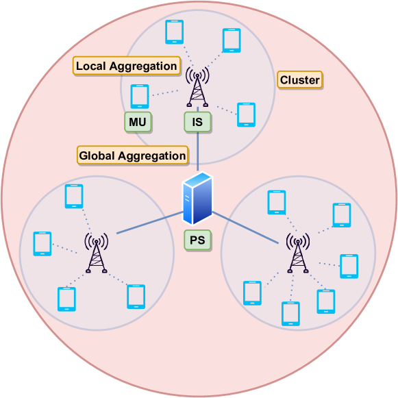
In order to make distant MUs more resilient to the channel effects, we propose hierarchical over-the-air federated learning (HOTAFL), where MUs communicate with their corresponding ISs through wireless links. In this setup, each MU shares its local training result with its corresponding IS through OTA (cluster) aggregation. After several local iterations with the MUs in their clusters, the ISs send the results to the PS to complete the global aggregation, which constitutes one global iteration. We examine the performance of HOTAFL and compare the results with those of the conventional FL and error-free HFL both through analytical results and numerical experiments. The results show that the proposed framework outperforms conventional OTA FL and leads to a better model accuracy and faster convergence.

The paper is organized as follows: in Sections II and III, we introduce the HOTAFL framework as well as its communication model. In Section IV, we provide a convergence analysis of HOTAFL under convexity assumptions on the loss functions. We present our numerical results in Section V, and conclude the paper in Section VI.

II System Model

The objective of HOTAFL is to minimize a loss function F(𝜽)𝐹𝜽F(\bm{\theta}) with respect to the model weight vector 𝜽2N𝜽superscript2𝑁\bm{\theta}\in\mathbb{R}^{2N}, where 2N2𝑁2N is the model dimension. Our system consists of C𝐶C clusters each containing an IS and M𝑀M MUs as depicted in Fig. 1.

Refer to caption
Figure 1: HOTAFL system model.

The dataset of the m𝑚m-th MU in the c𝑐c-th cluster is denoted as m,csubscript𝑚𝑐\mathcal{B}_{m,c}, and we define Bc=1Cm=1M|m,c|𝐵superscriptsubscript𝑐1𝐶superscriptsubscript𝑚1𝑀subscript𝑚𝑐B\triangleq\sum_{c=1}^{C}\sum_{m=1}^{M}|\mathcal{B}_{m,c}|. We have

F(𝜽)=c=1Cm=1M|m,c|BFm,c(𝜽),𝐹𝜽superscriptsubscript𝑐1𝐶superscriptsubscript𝑚1𝑀subscript𝑚𝑐𝐵subscript𝐹𝑚𝑐𝜽F(\bm{\theta})=\sum_{c=1}^{C}\sum_{m=1}^{M}\frac{|\mathcal{B}_{m,c}|}{B}F_{m,c}(\bm{\theta}), (1)

where Fm,c(𝜽)1|m,c|um,cf(𝜽,u)subscript𝐹𝑚𝑐𝜽1subscript𝑚𝑐subscript𝑢subscript𝑚𝑐𝑓𝜽𝑢F_{m,c}(\bm{\theta})\triangleq\frac{1}{|\mathcal{B}_{m,c}|}\sum_{u\in\mathcal{B}_{m,c}}f(\bm{\theta},u), with f(𝜽,u)𝑓𝜽𝑢f(\bm{\theta},u) denoting the corresponding loss of u𝑢u-th data sample.

We consider a hierarchical and iterative approach to minimize (1) consisting of global, local, and user iterations. In every cluster iteration, the MUs carry out τ𝜏\tau user iterations on their own, then send their model updates to their corresponding ISs for local iteration. I𝐼I local iterations are performed at the IS in every cluster before all the local models are forwarded to the PS for global aggregation. At the j𝑗j-th user iteration of the i𝑖i-th local iteration, the weight update is performed employing stochastic gradient descent (SGD) for the m𝑚m-th user in the c𝑐c-th cluster as follows

𝜽m,ci,j+1(t)=𝜽m,ci,j(t)ηm,ci,j(t)Fm,c(𝜽m,ci,j(t),𝝃m,ci,j(t)),superscriptsubscript𝜽𝑚𝑐𝑖𝑗1𝑡superscriptsubscript𝜽𝑚𝑐𝑖𝑗𝑡superscriptsubscript𝜂𝑚𝑐𝑖𝑗𝑡subscript𝐹𝑚𝑐superscriptsubscript𝜽𝑚𝑐𝑖𝑗𝑡superscriptsubscript𝝃𝑚𝑐𝑖𝑗𝑡\bm{\theta}_{m,c}^{i,j+1}(t)=\bm{\theta}_{m,c}^{i,j}(t)-\eta_{m,c}^{i,j}(t)\nabla F_{m,c}(\bm{\theta}_{m,c}^{i,j}(t),\bm{\xi}_{m,c}^{i,j}(t)), (2)

where ηm,ci,j(t)superscriptsubscript𝜂𝑚𝑐𝑖𝑗𝑡\eta_{m,c}^{i,j}(t) is the learning rate, Fm,c(𝜽m,ci,j(t),𝝃m,ci,j(t))subscript𝐹𝑚𝑐superscriptsubscript𝜽𝑚𝑐𝑖𝑗𝑡superscriptsubscript𝝃𝑚𝑐𝑖𝑗𝑡\nabla F_{m,c}(\bm{\theta}_{m,c}^{i,j}(t),\bm{\xi}_{m,c}^{i,j}(t)) denotes the stochastic gradient estimate for the weight vector 𝜽m,ci,j(t)superscriptsubscript𝜽𝑚𝑐𝑖𝑗𝑡\bm{\theta}_{m,c}^{i,j}(t) and a randomly sampled batch of data samples ξm,ci,j(t)superscriptsubscript𝜉𝑚𝑐𝑖𝑗𝑡\xi_{m,c}^{i,j}(t) from the dataset of the m𝑚m-th user in the c𝑐c-th cluster at the t𝑡t-th global, i𝑖i-th local and j𝑗j-th user iteration. Initially, 𝜽m,c1,1(t)=𝜽IS,ci(t),i[I]formulae-sequencesuperscriptsubscript𝜽𝑚𝑐11𝑡superscriptsubscript𝜽𝐼𝑆𝑐𝑖𝑡for-all𝑖delimited-[]𝐼\bm{\theta}_{m,c}^{1,1}(t)=\bm{\theta}_{IS,c}^{i}(t),\forall i\in[I] where [I]{1,2,,I}delimited-[]𝐼12𝐼[I]\triangleq\{1,2,\ldots,I\}, and 𝜽IS,c1(t)=𝜽PS(t)superscriptsubscript𝜽𝐼𝑆𝑐1𝑡subscript𝜽𝑃𝑆𝑡\bm{\theta}_{IS,c}^{1}(t)=\bm{\theta}_{PS}(t), where 𝜽PS(t)subscript𝜽𝑃𝑆𝑡\bm{\theta}_{PS}(t) is the global model at the PS at the t𝑡t-th global iteration and 𝜽IS,ci(t)superscriptsubscript𝜽𝐼𝑆𝑐𝑖𝑡\bm{\theta}_{IS,c}^{i}(t) denotes the local model of IS in the c𝑐c-th cluster at the i𝑖i-th local iteration. The purpose of employing ISs is to accumulate the local model differences within each cluster more frequently in smaller areas before obtaining the global model 𝜽PS(t)subscript𝜽𝑃𝑆𝑡\bm{\theta}_{PS}(t) for the next iteration. Also, note that Fm,c(𝜽m,ci,j(t),𝝃m,ci,j(t))subscript𝐹𝑚𝑐superscriptsubscript𝜽𝑚𝑐𝑖𝑗𝑡superscriptsubscript𝝃𝑚𝑐𝑖𝑗𝑡\nabla F_{m,c}(\bm{\theta}_{m,c}^{i,j}(t),\bm{\xi}_{m,c}^{i,j}(t)) is an unbiased estimator of Fm,c(𝜽m,ci,j(t))subscript𝐹𝑚𝑐superscriptsubscript𝜽𝑚𝑐𝑖𝑗𝑡\nabla F_{m,c}(\bm{\theta}_{m,c}^{i,j}(t)), i.e., 𝔼ξ[Fm,c(𝜽m,ci,j(t),𝝃m,ci,j(t))]=Fm,c(𝜽m,ci,j(t)),subscript𝔼𝜉delimited-[]subscript𝐹𝑚𝑐superscriptsubscript𝜽𝑚𝑐𝑖𝑗𝑡superscriptsubscript𝝃𝑚𝑐𝑖𝑗𝑡subscript𝐹𝑚𝑐superscriptsubscript𝜽𝑚𝑐𝑖𝑗𝑡\mathbb{E}_{\xi}\left[\nabla F_{m,c}(\bm{\theta}_{m,c}^{i,j}(t),\bm{\xi}_{m,c}^{i,j}(t))\right]=\nabla F_{m,c}(\bm{\theta}_{m,c}^{i,j}(t)), where the expectation is over the randomness due to the SGD.

III Hierarchical Over-the-Air FL (HOTAFL)

III-A Ideal Communication

We refer to the case where all the communication among all the units is error-free as the ideal communication scenario. In this case, after performing SGD, each MU calculates its model difference to be sent to its corresponding IS as

Δ𝜽m,ci(t)=𝜽m,ci,τ+1(t)𝜽IS,ci(t).Δsuperscriptsubscript𝜽𝑚𝑐𝑖𝑡superscriptsubscript𝜽𝑚𝑐𝑖𝜏1𝑡superscriptsubscript𝜽𝐼𝑆𝑐𝑖𝑡\Delta\bm{\theta}_{m,c}^{i}(t)=\bm{\theta}_{m,c}^{i,\tau+1}(t)-\bm{\theta}_{IS,c}^{i}(t). (3)

Then, the local aggregation at the c𝑐c-th cluster is performed as

Δ𝜽IS,ci(t)Δsuperscriptsubscript𝜽𝐼𝑆𝑐𝑖𝑡\displaystyle\Delta\bm{\theta}_{IS,c}^{i}(t) =1Mm=1MΔ𝜽m,ci(t),absent1𝑀superscriptsubscript𝑚1𝑀Δsuperscriptsubscript𝜽𝑚𝑐𝑖𝑡\displaystyle=\frac{1}{M}\sum_{m=1}^{M}\Delta\bm{\theta}_{m,c}^{i}(t), (4)
𝜽IS,ci+1(t)superscriptsubscript𝜽𝐼𝑆𝑐𝑖1𝑡\displaystyle\bm{\theta}_{IS,c}^{i+1}(t) =𝜽IS,ci(t)+Δ𝜽IS,ci(t).absentsuperscriptsubscript𝜽𝐼𝑆𝑐𝑖𝑡Δsuperscriptsubscript𝜽𝐼𝑆𝑐𝑖𝑡\displaystyle=\bm{\theta}_{IS,c}^{i}(t)+\Delta\bm{\theta}_{IS,c}^{i}(t). (5)

After completing I𝐼I local iterations in each cluster, ISs send their model updates to the PS, which can be written as

Δ𝜽PS,c(t)=𝜽IS,cI+1(t)𝜽PS(t).Δsubscript𝜽𝑃𝑆𝑐𝑡superscriptsubscript𝜽𝐼𝑆𝑐𝐼1𝑡subscript𝜽𝑃𝑆𝑡\Delta\bm{\theta}_{PS,c}(t)=\bm{\theta}_{IS,c}^{I+1}(t)-\bm{\theta}_{PS}(t). (6)

The global update rule is Δ𝜽PS(t)=1Cc=1CΔ𝜽PS,c(t)Δsubscript𝜽𝑃𝑆𝑡1𝐶superscriptsubscript𝑐1𝐶Δsubscript𝜽𝑃𝑆𝑐𝑡\Delta\bm{{\theta}}_{PS}(t)=\frac{1}{C}\sum_{c=1}^{C}\Delta\bm{\theta}_{PS,c}(t). Using recursion, we can conclude that

Δ𝜽PS(t)=1MCc=1Ci=1Im=1MΔ𝜽m,ci(t).Δsubscript𝜽𝑃𝑆𝑡1𝑀𝐶superscriptsubscript𝑐1𝐶superscriptsubscript𝑖1𝐼superscriptsubscript𝑚1𝑀Δsuperscriptsubscript𝜽𝑚𝑐𝑖𝑡\Delta\bm{\theta}_{PS}(t)=\frac{1}{MC}\sum_{c=1}^{C}\sum_{i=1}^{I}\sum_{m=1}^{M}\Delta\bm{\theta}_{m,c}^{i}(t). (7)

After the global aggregation, the model at the PS is updated as 𝜽PS(t+1)=𝜽PS(t)+Δ𝜽PS(t)subscript𝜽𝑃𝑆𝑡1subscript𝜽𝑃𝑆𝑡Δsubscript𝜽𝑃𝑆𝑡\bm{\theta}_{PS}(t+1)=\bm{\theta}_{PS}(t)+\Delta\bm{\theta}_{PS}(t).

III-B OTA Communication

We now consider the scheme referred as OTA communications, for which the links between the users and the ISs are wireless with OTA aggregation, however, the links between ISs and the PS is assumed to be error-free. Since a common wireless medium is used in local aggregations, noisy versions of the model updates Δ𝜽IS,c(t)Δsubscript𝜽𝐼𝑆𝑐𝑡\Delta\bm{\theta}_{IS,c}(t) are received at the ISs. In our setup, the ISs are equipped with K𝐾K antennas, and we assume perfect channel state information (CSI) at the receivers. For the k𝑘k-th antenna, the received signal at the c𝑐c-th IS can be written as111Note that the setup here can be efficiently implemented in practice using orthogonal frequency-division multiplexing (OFDM).

𝒚IS,c,ki(t)=m=1M𝒉m,c,ki(t)𝒙m,c,ki(t)+𝒛IS,c,ki(t),superscriptsubscript𝒚𝐼𝑆𝑐𝑘𝑖𝑡superscriptsubscript𝑚1𝑀superscriptsubscript𝒉𝑚𝑐𝑘𝑖𝑡superscriptsubscript𝒙𝑚𝑐𝑘𝑖𝑡superscriptsubscript𝒛𝐼𝑆𝑐𝑘𝑖𝑡\bm{y}_{IS,c,k}^{i}(t)=\sum_{m=1}^{M}\bm{h}_{m,c,k}^{i}(t)\circ\bm{x}_{m,c,k}^{i}(t)+\bm{z}_{IS,c,k}^{i}(t), (8)

where \circ denotes the element-wise product, 𝒙m,c,ki(t)Nsuperscriptsubscript𝒙𝑚𝑐𝑘𝑖𝑡superscript𝑁\bm{x}_{m,c,k}^{i}(t)\in\mathbb{C}^{N}, 𝒛IS,c,ki(t)Nsuperscriptsubscript𝒛𝐼𝑆𝑐𝑘𝑖𝑡superscript𝑁\bm{z}_{IS,c,k}^{i}(t)\in\mathbb{C}^{N} with independent and identically distributed (i.i.d.) entries zIS,c,ki,n(t)𝒞𝒩(0,σz2)similar-tosuperscriptsubscript𝑧𝐼𝑆𝑐𝑘𝑖𝑛𝑡𝒞𝒩0superscriptsubscript𝜎𝑧2z_{IS,c,k}^{i,n}(t)\sim\mathcal{CN}(0,\sigma_{z}^{2}). The channel coefficients are modelled as 𝒉m,c,ki(t)=βm,c𝒈m,c,ki(t)superscriptsubscript𝒉𝑚𝑐𝑘𝑖𝑡subscript𝛽𝑚𝑐superscriptsubscript𝒈𝑚𝑐𝑘𝑖𝑡\bm{h}_{m,c,k}^{i}(t)=\sqrt{\beta_{m,c}}~{}\bm{g}_{m,c,k}^{i}(t), where 𝒈m,c,k(t)Nsubscript𝒈𝑚𝑐𝑘𝑡superscript𝑁\bm{g}_{m,c,k}(t)\in\mathbb{C}^{N} with entries gm,c,ki,n(t)𝒞𝒩(0,σh2)similar-tosuperscriptsubscript𝑔𝑚𝑐𝑘𝑖𝑛𝑡𝒞𝒩0superscriptsubscript𝜎2g_{m,c,k}^{i,n}(t)\sim\mathcal{CN}(0,\sigma_{h}^{2}) (i.e., Rayleigh fading), βm,csubscript𝛽𝑚𝑐\beta_{m,c} is the large-scale fading coefficient modeled as βm,c=(dm,c)psubscript𝛽𝑚𝑐superscriptsubscript𝑑𝑚𝑐𝑝\beta_{m,c}=\left(d_{m,c}\right)^{-p}, where p𝑝p represents the path loss exponent, and dm,csubscript𝑑𝑚𝑐d_{m,c} denotes the distance between the m𝑚m-th user in the c𝑐c-th cluster and the IS in that cluster.

III-B1 Local Aggregation

In OTA communication, in order to increase the spectral efficiency, the model differences are grouped to form a complex vector Δ𝜽m,ci,cxNΔsuperscriptsubscript𝜽𝑚𝑐𝑖𝑐𝑥superscript𝑁\Delta\bm{\theta}_{m,c}^{i,cx}\in\mathbb{C}^{N} with the following real and imaginary parts

Δ𝜽m,ci,re(t)[Δθm,ci,1(t),Δθm,ci,2(t),,Δθm,ci,N(t)]T,Δsuperscriptsubscript𝜽𝑚𝑐𝑖𝑟𝑒𝑡superscriptΔsuperscriptsubscript𝜃𝑚𝑐𝑖1𝑡Δsuperscriptsubscript𝜃𝑚𝑐𝑖2𝑡Δsuperscriptsubscript𝜃𝑚𝑐𝑖𝑁𝑡𝑇\displaystyle\!\!\Delta\bm{\theta}_{m,c}^{i,re}(t)\triangleq\left[\Delta\theta_{m,c}^{i,1}(t),\Delta\theta_{m,c}^{i,2}(t),\ldots,\Delta\theta_{m,c}^{i,N}(t)\right]^{T}, (9a)
Δ𝜽m,ci,im(t)[Δθm,ci,N+1(t),Δθm,ci,N+2(t),,Δθm,ci,2N(t)]T.Δsuperscriptsubscript𝜽𝑚𝑐𝑖𝑖𝑚𝑡superscriptΔsuperscriptsubscript𝜃𝑚𝑐𝑖𝑁1𝑡Δsuperscriptsubscript𝜃𝑚𝑐𝑖𝑁2𝑡Δsuperscriptsubscript𝜃𝑚𝑐𝑖2𝑁𝑡𝑇\displaystyle\!\!\Delta\bm{\theta}_{m,c}^{i,im}(t)\!\triangleq\!\!\left[\Delta\theta_{m,c}^{i,N+1}\!(t),\Delta\theta_{m,c}^{i,N+2}(t),\ldots,\Delta\theta_{m,c}^{i,2N}\!(t)\!\right]^{\!T}\!\!. (9b)

Under the assumption that there is no inter-cluster interference, the received signal for the k𝑘k-th antenna in the c𝑐c-th cluster at the i𝑖i-th local iteration can be represented as

𝒚IS,c,ki(t)=Ptm=1M𝒉m,c,ki(t)Δ𝜽m,ci,cx(t)+𝒛IS,c,ki(t),superscriptsubscript𝒚𝐼𝑆𝑐𝑘𝑖𝑡subscript𝑃𝑡superscriptsubscript𝑚1𝑀superscriptsubscript𝒉𝑚𝑐𝑘𝑖𝑡Δsuperscriptsubscript𝜽𝑚𝑐𝑖𝑐𝑥𝑡superscriptsubscript𝒛𝐼𝑆𝑐𝑘𝑖𝑡\bm{y}_{IS,c,k}^{i}(t)=P_{t}\sum_{m=1}^{M}\bm{h}_{m,c,k}^{i}(t)\circ\Delta\bm{\theta}_{m,c}^{i,cx}(t)+\bm{z}_{IS,c,k}^{i}(t), (10)

where Ptsubscript𝑃𝑡P_{t} is the transmit power constant at the t𝑡t-th global iteration. Knowing the CSI perfectly, the c𝑐c-th IS combines the received signals as 𝒚IS,ci(t)=1Kk=1K(m=1M𝒉m,c,ki(t))𝒚IS,c,ki(t)superscriptsubscript𝒚𝐼𝑆𝑐𝑖𝑡1𝐾superscriptsubscript𝑘1𝐾superscriptsuperscriptsubscript𝑚1𝑀superscriptsubscript𝒉𝑚𝑐𝑘𝑖𝑡superscriptsubscript𝒚𝐼𝑆𝑐𝑘𝑖𝑡\bm{y}_{IS,c}^{i}(t)\!=\!\frac{1}{K}\!\sum_{k=1}^{K}\!\Big{(}\!\sum_{m=1}^{M}\bm{h}_{m,c,k}^{i}(t)\Big{)}^{\!\!\ast}\!\circ\!\bm{y}_{IS,c,k}^{i}(t). For the n𝑛n-th symbol, it can be written as

yIS,ci,n(t)superscriptsubscript𝑦𝐼𝑆𝑐𝑖𝑛𝑡\displaystyle y_{IS,c}^{i,n}(t)\! =Ptm=1M(1Kk=1K|hm,c,ki,n(t)|2)Δθm,ci,n,cx(t)yIS,ci,n,sig(t) (signal term)absentsubscriptsubscript𝑃𝑡superscriptsubscript𝑚1𝑀1𝐾superscriptsubscript𝑘1𝐾superscriptsuperscriptsubscript𝑚𝑐𝑘𝑖𝑛𝑡2Δsuperscriptsubscript𝜃𝑚𝑐𝑖𝑛𝑐𝑥𝑡yIS,ci,n,sig(t) (signal term)\displaystyle=\!\underbrace{P_{t}\!\sum_{m=1}^{M}\!\Big{(}\!\frac{1}{K}\!\sum_{k=1}^{K}\lvert h_{m,c,k}^{i,n}(t)\rvert^{2}\!\Big{)}\!\Delta\theta_{m,c}^{i,n,cx}(t)}_{\text{$y_{IS,c}^{i,n,sig}(t)$ (signal term)}}
+PtKm=1Mm=1mmMk=1K(hm,c,ki,n(t))hm,c,ki,n(t)Δθm,ci,n,cx(t)yIS,ci,n,itf(t) (interference term)subscriptsubscript𝑃𝑡𝐾superscriptsubscript𝑚1𝑀superscriptsubscriptsuperscript𝑚1superscript𝑚𝑚𝑀superscriptsubscript𝑘1𝐾superscriptsuperscriptsubscript𝑚𝑐𝑘𝑖𝑛𝑡superscriptsubscriptsuperscript𝑚𝑐𝑘𝑖𝑛𝑡Δsuperscriptsubscript𝜃superscript𝑚𝑐𝑖𝑛𝑐𝑥𝑡yIS,ci,n,itf(t) (interference term)\displaystyle\hskip 8.5359pt+\underbrace{\frac{P_{t}}{K}\!\sum_{m=1}^{M}\!\sum_{\begin{subarray}{c}m^{\prime}=1\\ m^{\prime}\neq m\end{subarray}}^{M}\!\sum_{k=1}^{K}\!(h_{m,c,k}^{i,n}(t))^{\ast}\!h_{m^{\prime},c,k}^{i,n}(t)\Delta\theta_{m^{\prime},c}^{i,n,cx}(t)}_{\text{$y_{IS,c}^{i,n,itf}(t)$ (interference term)}}
+1Km=1Mk=1K(hm,c,ki,n(t))zc,ki,n(t)yIS,ci,n,no(t) (noise term).subscript1𝐾superscriptsubscript𝑚1𝑀superscriptsubscript𝑘1𝐾superscriptsuperscriptsubscript𝑚𝑐𝑘𝑖𝑛𝑡superscriptsubscript𝑧𝑐𝑘𝑖𝑛𝑡yIS,ci,n,no(t) (noise term)\displaystyle\hskip 8.5359pt+\underbrace{\frac{1}{K}\!\sum_{m=1}^{M}\!\sum_{k=1}^{K}(h_{m,c,k}^{i,n}(t))^{\ast}z_{c,k}^{i,n}(t)}_{\text{$y_{IS,c}^{i,n,no}(t)$ (noise term)}}. (11)

Aggregated model differences can be recovered by

Δθ^IS,ci,n(t)Δsuperscriptsubscript^𝜃𝐼𝑆𝑐𝑖𝑛𝑡\displaystyle\Delta\hat{\theta}_{IS,c}^{i,n}(t) =1PtMσh2β¯cRe{yIS,ci,n(t)},absent1subscript𝑃𝑡𝑀superscriptsubscript𝜎2subscript¯𝛽𝑐Resuperscriptsubscript𝑦𝐼𝑆𝑐𝑖𝑛𝑡\displaystyle=\frac{1}{P_{t}M\sigma_{h}^{2}\bar{\beta}_{c}}\operatorname{Re}\{y_{IS,c}^{i,n}(t)\}, (12a)
Δθ^IS,ci,n+N(t)Δsuperscriptsubscript^𝜃𝐼𝑆𝑐𝑖𝑛𝑁𝑡\displaystyle\Delta\hat{\theta}_{IS,c}^{i,n+N}(t) =1PtMσh2β¯cIm{yIS,ci,n(t)},absent1subscript𝑃𝑡𝑀superscriptsubscript𝜎2subscript¯𝛽𝑐Imsuperscriptsubscript𝑦𝐼𝑆𝑐𝑖𝑛𝑡\displaystyle=\frac{1}{P_{t}M\sigma_{h}^{2}\bar{\beta}_{c}}\operatorname{Im}\{y_{IS,c}^{i,n}(t)\}, (12b)

where β¯c=m=1Mβm,csubscript¯𝛽𝑐superscriptsubscript𝑚1𝑀subscript𝛽𝑚𝑐\bar{\beta}_{c}=\sum_{m=1}^{M}\beta_{m,c}. After estimating the model difference values, the cluster model update is written as

𝜽IS,ci+1(t)=𝜽IS,ci(t)+Δ𝜽^IS,ci(t),superscriptsubscript𝜽𝐼𝑆𝑐𝑖1𝑡superscriptsubscript𝜽𝐼𝑆𝑐𝑖𝑡Δsuperscriptsubscriptbold-^𝜽𝐼𝑆𝑐𝑖𝑡\bm{\theta}_{IS,c}^{i+1}(t)=\bm{\theta}_{IS,c}^{i}(t)+\Delta\bm{\hat{\theta}}_{IS,c}^{i}(t), (13)

where Δ𝜽^IS,ci(t)=[Δθ^IS,ci,1(t)Δθ^IS,ci,2(t)Δθ^IS,ci,2N(t)]TΔsuperscriptsubscriptbold-^𝜽𝐼𝑆𝑐𝑖𝑡superscriptdelimited-[]Δsuperscriptsubscript^𝜃𝐼𝑆𝑐𝑖1𝑡Δsuperscriptsubscript^𝜃𝐼𝑆𝑐𝑖2𝑡Δsuperscriptsubscript^𝜃𝐼𝑆𝑐𝑖2𝑁𝑡𝑇\Delta\bm{\hat{\theta}}_{IS,c}^{i}(t)=\big{[}\Delta\hat{\theta}_{IS,c}^{i,1}(t)~{}\Delta\hat{\theta}_{IS,c}^{i,2}(t)~{}\cdots~{}\Delta\hat{\theta}_{IS,c}^{i,2N}(t)\big{]}^{T}.

III-B2 Global Aggregation

This part is similar to the case of ideal communication. The only difference is that the aggregated signals are estimates of the actual model differences. Letting 𝒙PS,c(t)subscript𝒙𝑃𝑆𝑐𝑡\bm{x}_{PS,c}(t) be the transmitted signal from the c𝑐c-th IS, its n𝑛n-th symbol can be written as

xPS,cn(t)=ΔθPS,cn(t)+jΔθPS,cn+N(t).superscriptsubscript𝑥𝑃𝑆𝑐𝑛𝑡Δsuperscriptsubscript𝜃𝑃𝑆𝑐𝑛𝑡𝑗Δsuperscriptsubscript𝜃𝑃𝑆𝑐𝑛𝑁𝑡\displaystyle x_{PS,c}^{n}(t)=\Delta\theta_{PS,c}^{n}(t)+j\Delta\theta_{PS,c}^{n+N}(t). (14)

Then, using (6), (11), (14) and recursion, the received signal for 1nN1𝑛𝑁1\!\leq\!n\!\leq\!N (similarly for N+1n2N𝑁1𝑛2𝑁N\!+\!1\!\leq\!n\!\leq\!2N) can be written as

yPSn(t)=c=1CxPS,cn(t)superscriptsubscript𝑦𝑃𝑆𝑛𝑡superscriptsubscript𝑐1𝐶superscriptsubscript𝑥𝑃𝑆𝑐𝑛𝑡\displaystyle y_{PS}^{n}(t)=\sum_{c=1}^{C}x_{PS,c}^{n}(t) (15)
=c=1Ci=1IRe{yIS,ci,n,sig(t)}PtMσh2yPS,1n(t)+c=1Ci=1IRe{yIS,ci,n,itf(t)}PtMσh2yPS,2n(t)absentsubscriptsuperscriptsubscript𝑐1𝐶superscriptsubscript𝑖1𝐼Resuperscriptsubscript𝑦𝐼𝑆𝑐𝑖𝑛𝑠𝑖𝑔𝑡subscript𝑃𝑡𝑀superscriptsubscript𝜎2superscriptsubscript𝑦𝑃𝑆1𝑛𝑡subscriptsuperscriptsubscript𝑐1𝐶superscriptsubscript𝑖1𝐼Resuperscriptsubscript𝑦𝐼𝑆𝑐𝑖𝑛𝑖𝑡𝑓𝑡subscript𝑃𝑡𝑀superscriptsubscript𝜎2superscriptsubscript𝑦𝑃𝑆2𝑛𝑡\displaystyle=\!\!\!\underbrace{\sum_{c=1}^{C}\!\sum_{i=1}^{I}\!\frac{\operatorname{Re}\big{\{}y_{IS,c}^{i,n,sig}(t)\big{\}}}{P_{t}M\sigma_{h}^{2}}}_{y_{PS,1}^{n}(t)}\!+\!\underbrace{\sum_{c=1}^{C}\!\sum_{i=1}^{I}\!\frac{\operatorname{Re}\big{\{}y_{IS,c}^{i,n,itf}(t)\big{\}}}{P_{t}M\sigma_{h}^{2}}}_{y_{PS,2}^{n}(t)}
+c=1Ci=1IRe{yIS,ci,n,no(t)}PtMσh2yPS,3n(t).subscriptsuperscriptsubscript𝑐1𝐶superscriptsubscript𝑖1𝐼Resuperscriptsubscript𝑦𝐼𝑆𝑐𝑖𝑛𝑛𝑜𝑡subscript𝑃𝑡𝑀superscriptsubscript𝜎2superscriptsubscript𝑦𝑃𝑆3𝑛𝑡\displaystyle\quad+\underbrace{\sum_{c=1}^{C}\!\sum_{i=1}^{I}\!\frac{\operatorname{Re}\big{\{}y_{IS,c}^{i,n,no}(t)\big{\}}}{P_{t}M\sigma_{h}^{2}}}_{y_{PS,3}^{n}(t)}\!. (16)

The received signal at the PS is then recovered as Δθ^PSn(t)=1CRe{yPSn(t)}Δsuperscriptsubscript^𝜃𝑃𝑆𝑛𝑡1𝐶Resuperscriptsubscript𝑦𝑃𝑆𝑛𝑡\Delta\hat{\theta}_{PS}^{n}(t)=\frac{1}{C}\operatorname{Re}\{y_{PS}^{n}(t)\}, Δθ^PSn+N(t)=1CIm{yPSn(t)}Δsuperscriptsubscript^𝜃𝑃𝑆𝑛𝑁𝑡1𝐶Imsuperscriptsubscript𝑦𝑃𝑆𝑛𝑡\Delta\hat{\theta}_{PS}^{n+N}(t)=\frac{1}{C}\operatorname{Im}\{y_{PS}^{n}(t)\}. Finally, the global aggregation is performed as

𝜽PS(t+1)=𝜽PS(t)+Δ𝜽^PS(t),subscript𝜽𝑃𝑆𝑡1subscript𝜽𝑃𝑆𝑡Δsubscriptbold-^𝜽𝑃𝑆𝑡\displaystyle\bm{\theta}_{PS}(t+1)=\bm{\theta}_{PS}(t)+\Delta\bm{\hat{\theta}}_{PS}(t), (17)

where Δ𝜽^PS(t)=[Δθ^PS1(t)Δθ^PS2(t)Δθ^PS2N(t)]TΔsubscriptbold-^𝜽𝑃𝑆𝑡superscriptdelimited-[]Δsuperscriptsubscript^𝜃𝑃𝑆1𝑡Δsuperscriptsubscript^𝜃𝑃𝑆2𝑡Δsuperscriptsubscript^𝜃𝑃𝑆2𝑁𝑡𝑇\Delta\bm{\hat{\theta}}_{PS}(t)=\big{[}\Delta\hat{\theta}_{PS}^{1}(t)~{}\Delta\hat{\theta}_{PS}^{2}(t)~{}\cdots~{}\Delta\hat{\theta}_{PS}^{2N}(t)\big{]}^{T}.

IV Convergence Analysis

In this section, we present a convergence analysis of the proposed HOTAFL algorithm. Define the optimal solution as 𝜽argmin𝜽F(𝜽)superscript𝜽subscriptargmin𝜽𝐹𝜽\bm{\theta}^{\ast}\triangleq\operatorname*{arg\,min}_{\bm{\theta}}F(\bm{\theta}), the minimum values of the total and the local loss functions as F=F(𝜽)superscript𝐹𝐹superscript𝜽F^{*}=F(\bm{\theta}^{*}) and Fm,csuperscriptsubscript𝐹𝑚𝑐F_{m,c}^{*}, respectively, and the bias in the dataset as ΓFc=1Cm=1MBm,cBFm,c0Γsuperscript𝐹superscriptsubscript𝑐1𝐶superscriptsubscript𝑚1𝑀subscript𝐵𝑚𝑐𝐵superscriptsubscript𝐹𝑚𝑐0\Gamma\triangleq F^{*}-\sum_{c=1}^{C}\sum_{m=1}^{M}\frac{B_{m,c}}{B}F_{m,c}^{*}\geq 0. In addition, assume that the learning rate of the overall system does not change in local iterations, i.e., ηm,ci,j(t)=η(t)superscriptsubscript𝜂𝑚𝑐𝑖𝑗𝑡𝜂𝑡\eta_{m,c}^{i,j}(t)=\eta(t). Therefore, we can write the global update rule as

𝜽m,ci,j+1(t)superscriptsubscript𝜽𝑚𝑐𝑖𝑗1𝑡\displaystyle\bm{\theta}_{m,c}^{i,j+1}(t) =𝜽m,ci,j(t)η(t)Fm,c(𝜽m,ci,j(t),𝝃m,ci,j(t)),absentsuperscriptsubscript𝜽𝑚𝑐𝑖𝑗𝑡𝜂𝑡subscript𝐹𝑚𝑐superscriptsubscript𝜽𝑚𝑐𝑖𝑗𝑡superscriptsubscript𝝃𝑚𝑐𝑖𝑗𝑡\displaystyle=\bm{\theta}_{m,c}^{i,j}(t)-\eta(t)\nabla F_{m,c}(\bm{\theta}_{m,c}^{i,j}(t),\bm{\xi}_{m,c}^{i,j}(t)), (18)

which can also be written as

𝜽m,ci,j+1(t)𝜽m,ci,1(t)=η(t)l=1jFm,c(𝜽m,ci,l,𝝃m,ci,l(t)).superscriptsubscript𝜽𝑚𝑐𝑖𝑗1𝑡superscriptsubscript𝜽𝑚𝑐𝑖1𝑡𝜂𝑡superscriptsubscript𝑙1𝑗subscript𝐹𝑚𝑐superscriptsubscript𝜽𝑚𝑐𝑖𝑙superscriptsubscript𝝃𝑚𝑐𝑖𝑙𝑡\bm{\theta}_{m,c}^{i,j+1}(t)-\bm{\theta}_{m,c}^{i,1}(t)=-\eta(t)\sum_{l=1}^{j}\nabla F_{m,c}(\bm{\theta}_{m,c}^{i,l},\bm{\xi}_{m,c}^{i,l}(t)). (19)
Assumption 1.

All the loss functions are L-smooth and μ𝜇\mu-strongly convex; i.e., 𝐯,𝐰2Nfor-all𝐯𝐰superscript2𝑁\forall\bm{v},\bm{w}\in\mathbb{R}^{2N}, m[M],c[C]formulae-sequencefor-all𝑚delimited-[]𝑀for-all𝑐delimited-[]𝐶\forall m\in[M],\forall c\in[C],

Fm,c(𝒗)Fm,c(𝒘)subscript𝐹𝑚𝑐𝒗subscript𝐹𝑚𝑐𝒘\displaystyle\!\!F_{m,c}(\bm{v})\!-\!F_{m,c}(\bm{w}) 𝒗𝒘,Fm,c(𝒘)+L2𝒗𝒘22,absent𝒗𝒘subscript𝐹𝑚𝑐𝒘𝐿2superscriptsubscriptnorm𝒗𝒘22\displaystyle\!\leq\!\langle\bm{v}\!-\!\bm{w},\!\nabla\!F_{m,c}(\bm{w})\rangle\!+\!\frac{L}{2}\!\left\|\bm{v}-\bm{w}\right\|_{2}^{2}\!, (20)
Fm,c(𝒗)Fm,c(𝒘)subscript𝐹𝑚𝑐𝒗subscript𝐹𝑚𝑐𝒘\displaystyle\!\!F_{m,c}(\bm{v})\!-\!F_{m,c}(\bm{w}) 𝒗𝒘,Fm,c(𝒘)+μ2𝒗𝒘22.absent𝒗𝒘subscript𝐹𝑚𝑐𝒘𝜇2superscriptsubscriptnorm𝒗𝒘22\displaystyle\!\geq\!\langle\bm{v}\!-\!\bm{w},\!\nabla\!F_{m,c}(\bm{w})\rangle\!+\!\frac{\mu}{2}\!\left\|\bm{v}-\bm{w}\right\|_{2}^{2}\!. (21)
Assumption 2.

The expected value of the squared l2subscript𝑙2l_{2} norm of the stochastic gradients are bounded; i.e., j[τ],i[I]formulae-sequencefor-all𝑗delimited-[]𝜏𝑖delimited-[]𝐼\forall j\in[\tau],i\in[I],

𝔼ξ[Fm,c(𝜽m,ci,j(t),𝝃m,ci,j(t))22]G2,subscript𝔼𝜉delimited-[]superscriptsubscriptnormsubscript𝐹𝑚𝑐superscriptsubscript𝜽𝑚𝑐𝑖𝑗𝑡superscriptsubscript𝝃𝑚𝑐𝑖𝑗𝑡22superscript𝐺2\mathbb{E}_{\xi}\Big{[}\left\|\nabla F_{m,c}(\bm{\theta}_{m,c}^{i,j}(t),\bm{\xi}_{m,c}^{i,j}(t))\right\|_{2}^{2}\Big{]}\leq G^{2}, (22)

which translates to n[2N]for-all𝑛delimited-[]2𝑁\forall n\!\in\![2N], 𝔼ξ[Fm,c(θm,ci,j,n,ξm,ci,j,n(t))]Gsubscript𝔼𝜉delimited-[]subscript𝐹𝑚𝑐superscriptsubscript𝜃𝑚𝑐𝑖𝑗𝑛superscriptsubscript𝜉𝑚𝑐𝑖𝑗𝑛𝑡𝐺\mathbb{E}_{\xi}\!\!\left[\nabla\!F_{m,c}(\theta_{m,c}^{i,j,n},\xi_{m,c}^{i,j,n}(t))\!\right]\!\!\leq\!G.

Theorem 1.

In HOTAFL, for 0η(t)min{1,1μτI}0𝜂𝑡𝑚𝑖𝑛11𝜇𝜏𝐼0\leq\eta(t)\leq min\{1,\frac{1}{\mu\tau I}\}, the global loss function can be upper bounded as

𝔼[𝜽PS(t)𝜽22]𝔼delimited-[]superscriptsubscriptnormsubscript𝜽𝑃𝑆𝑡superscript𝜽22\displaystyle\mathbb{E}\big{[}\left\|\bm{\theta}_{PS}(t)-\bm{\theta}^{*}\right\|_{2}^{2}\big{]}
(a=1t1X(a))𝜽PS(0)𝜽22+b=1t1Y(b)a=b+1t1X(a),absentsuperscriptsubscriptproduct𝑎1𝑡1𝑋𝑎superscriptsubscriptnormsubscript𝜽𝑃𝑆0superscript𝜽22superscriptsubscript𝑏1𝑡1𝑌𝑏superscriptsubscriptproduct𝑎𝑏1𝑡1𝑋𝑎\displaystyle\leq\!\bigg{(}\prod_{a=1}^{t-1}\!X(a)\!\bigg{)}\!\left\|\bm{\theta}_{PS}(0)\!-\!\bm{\theta}^{*}\right\|_{2}^{2}\!+\!\sum_{b=1}^{t-1}\!Y(b)\!\prod_{a=b+1}^{t-1}\!X(a), (23)

where X(a)=(1μη(a)I(τη(a)(τ1)))𝑋𝑎1𝜇𝜂𝑎𝐼𝜏𝜂𝑎𝜏1X(a)=\left(1-\mu\eta(a)I\left(\tau-\eta(a)(\tau-1)\right)\right) and

Y(a)=𝑌𝑎absent\displaystyle Y(a)\!= η2(a)τ2G2IM2C2m1=1Mc1=1C(βm1,c12Kβc12¯+(m2=1Mc2=1CA1I))superscript𝜂2𝑎superscript𝜏2superscript𝐺2𝐼superscript𝑀2superscript𝐶2superscriptsubscriptsubscript𝑚11𝑀superscriptsubscriptsubscript𝑐11𝐶superscriptsubscript𝛽subscript𝑚1subscript𝑐12𝐾¯superscriptsubscript𝛽subscript𝑐12superscriptsubscriptsubscript𝑚21𝑀superscriptsubscriptsubscript𝑐21𝐶subscript𝐴1𝐼\displaystyle\frac{\eta^{2}(a)\tau^{2}G^{2}I}{M^{2}C^{2}}\!\!\sum_{m_{1}=1}^{M}\sum_{c_{1}=1}^{C}\!\Big{(}\frac{\beta_{m_{1},c_{1}}^{2}}{K\bar{\beta_{c_{1}}^{2}}}\!+\!\!\Big{(}\!\sum_{m_{2}=1}^{M}\sum_{c_{2}=1}^{C}A_{1}I\!\Big{)}\!\!\Big{)}
+m=1Mm=1mmMc=1Cη2(a)τ2G2Iβm,cβm,cM2C2Kβ¯c2superscriptsubscript𝑚1𝑀superscriptsubscriptsuperscript𝑚1superscript𝑚𝑚𝑀superscriptsubscript𝑐1𝐶superscript𝜂2𝑎superscript𝜏2superscript𝐺2𝐼subscript𝛽𝑚𝑐subscript𝛽superscript𝑚𝑐superscript𝑀2superscript𝐶2𝐾superscriptsubscript¯𝛽𝑐2\displaystyle+\sum_{m=1}^{M}\sum_{\begin{subarray}{c}m^{\prime}=1\\ m^{\prime}\neq m\end{subarray}}^{M}\sum_{c=1}^{C}\frac{\eta^{2}(a)\tau^{2}G^{2}I\beta_{m,c}\beta_{m^{\prime},c}}{M^{2}C^{2}K\bar{\beta}_{c}^{2}}
+σz2INPa2M2C2Kσh2m=1Mc=1Cβm,cβ¯c2superscriptsubscript𝜎𝑧2𝐼𝑁superscriptsubscript𝑃𝑎2superscript𝑀2superscript𝐶2𝐾superscriptsubscript𝜎2superscriptsubscript𝑚1𝑀superscriptsubscript𝑐1𝐶subscript𝛽𝑚𝑐superscriptsubscript¯𝛽𝑐2\displaystyle+\frac{\sigma_{z}^{2}IN}{P_{a}^{2}M^{2}C^{2}K\sigma_{h}^{2}}\sum_{m=1}^{M}\sum_{c=1}^{C}\frac{\beta_{m,c}}{\bar{\beta}_{c}^{2}}
+(1+μ(1η(a))η2(a)IG2τ(τ1)(2τ1)6\displaystyle+\left(1+\mu(1-\eta(a)\right)\eta^{2}(a)IG^{2}\frac{\tau(\tau-1)(2\tau-1)}{6}
+η2(a)I(τ2+τ1)G2+2η(a)I(τ1)Γ,superscript𝜂2𝑎𝐼superscript𝜏2𝜏1superscript𝐺22𝜂𝑎𝐼𝜏1Γ\displaystyle+\eta^{2}(a)I(\tau^{2}+\tau-1)G^{2}+2\eta(a)I(\tau-1)\Gamma, (24)

with A1=1βm1,c1β¯c1βm2,c2β¯c2+βm1,c1βm2,c2β¯c1β¯c2subscript𝐴11subscript𝛽subscript𝑚1subscript𝑐1subscript¯𝛽subscript𝑐1subscript𝛽subscript𝑚2subscript𝑐2subscript¯𝛽subscript𝑐2subscript𝛽subscript𝑚1subscript𝑐1subscript𝛽subscript𝑚2subscript𝑐2subscript¯𝛽subscript𝑐1subscript¯𝛽subscript𝑐2A_{1}=1-\frac{\beta_{m_{1},c_{1}}}{\bar{\beta}_{c_{1}}}-\frac{\beta_{m_{2},c_{2}}}{\bar{\beta}_{c_{2}}}+\frac{\beta_{m_{1},c_{1}}\beta_{m_{2},c_{2}}}{\bar{\beta}_{c_{1}}\bar{\beta}_{c_{2}}}.

Proof:

Let us define auxiliary variable 𝒗(t+1)=𝜽PS(t)+Δ𝜽PS(t)𝒗𝑡1subscript𝜽𝑃𝑆𝑡Δsubscript𝜽𝑃𝑆𝑡\bm{v}(t+1)=\bm{\theta}_{PS}(t)+\Delta\bm{\theta}_{PS}(t). Then, we have

𝜽PS(t+1)𝜽22=𝜽PS(t+1)𝒗(t+1)+𝒗(t+1)𝜽22superscriptsubscriptnormsubscript𝜽𝑃𝑆𝑡1superscript𝜽22superscriptsubscriptnormsubscript𝜽𝑃𝑆𝑡1𝒗𝑡1𝒗𝑡1superscript𝜽22\displaystyle\!\!\left\|\bm{\theta}_{PS}(t\!+\!1)\!-\!\bm{\theta}^{\ast}\right\|_{2}^{2}\!=\!\left\|\bm{\theta}_{PS}(t\!+\!1)\!-\!\bm{v}(t\!+\!1)+\bm{v}(t\!+\!1)\!-\!\bm{\theta}^{\ast}\right\|_{2}^{2}
=𝜽PS(t+1)𝒗(t+1)22+𝒗(t+1)𝜽22absentsuperscriptsubscriptnormsubscript𝜽𝑃𝑆𝑡1𝒗𝑡122superscriptsubscriptnorm𝒗𝑡1superscript𝜽22\displaystyle\!\!\quad=\left\|\bm{\theta}_{PS}(t+1)-\bm{v}(t+1)\right\|_{2}^{2}+\left\|\bm{v}(t+1)-\bm{\theta}^{\ast}\right\|_{2}^{2}
+2𝜽PS(t+1)𝒗(t+1),𝒗(t+1)𝜽.2subscript𝜽𝑃𝑆𝑡1𝒗𝑡1𝒗𝑡1superscript𝜽\displaystyle\!\!\quad\quad+2\langle\bm{\theta}_{PS}(t+1)-\bm{v}(t+1),\bm{v}(t+1)-\bm{\theta}^{\ast}\rangle. (25)

Next, we provide upper bounds on the three terms of (25).

Lemma 1.

We have

𝔼[𝜽PS(t+1)𝒗(t+1)22]𝔼delimited-[]superscriptsubscriptnormsubscript𝜽𝑃𝑆𝑡1𝒗𝑡122\displaystyle\mathbb{E}\Big{[}\big{\|}\bm{\theta}_{PS}(t+1)-\bm{v}(t+1)\big{\|}_{2}^{2}\Big{]}
η2(t)τ2G2IM2C2m1=1Mc1=1C(βm1,c12Kβc12¯+(m2=1Mc2=1CA1I))absentsuperscript𝜂2𝑡superscript𝜏2superscript𝐺2𝐼superscript𝑀2superscript𝐶2superscriptsubscriptsubscript𝑚11𝑀superscriptsubscriptsubscript𝑐11𝐶superscriptsubscript𝛽subscript𝑚1subscript𝑐12𝐾¯superscriptsubscript𝛽subscript𝑐12superscriptsubscriptsubscript𝑚21𝑀superscriptsubscriptsubscript𝑐21𝐶subscript𝐴1𝐼\displaystyle\leq\frac{\eta^{2}(t)\tau^{2}G^{2}I}{M^{2}C^{2}}\sum_{m_{1}=1}^{M}\sum_{c_{1}=1}^{C}\Big{(}\frac{\beta_{m_{1},c_{1}}^{2}}{K\bar{\beta_{c_{1}}^{2}}}+\Big{(}\sum_{m_{2}=1}^{M}\sum_{c_{2}=1}^{C}A_{1}I\Big{)}\Big{)}
+m=1Mm=1mmMc=1Cη2(t)τ2G2Iβm,cβm,cM2C2Kβ¯c2superscriptsubscript𝑚1𝑀superscriptsubscriptsuperscript𝑚1superscript𝑚𝑚𝑀superscriptsubscript𝑐1𝐶superscript𝜂2𝑡superscript𝜏2superscript𝐺2𝐼subscript𝛽𝑚𝑐subscript𝛽superscript𝑚𝑐superscript𝑀2superscript𝐶2𝐾superscriptsubscript¯𝛽𝑐2\displaystyle\quad+\sum_{m=1}^{M}\sum_{\begin{subarray}{c}m^{\prime}=1\\ m^{\prime}\neq m\end{subarray}}^{M}\sum_{c=1}^{C}\frac{\eta^{2}(t)\tau^{2}G^{2}I\beta_{m,c}\beta_{m^{\prime},c}}{M^{2}C^{2}K\bar{\beta}_{c}^{2}}
+σz2INPt2M2C2Kσh2m=1Mc=1Cβm,cβ¯c2.superscriptsubscript𝜎𝑧2𝐼𝑁superscriptsubscript𝑃𝑡2superscript𝑀2superscript𝐶2𝐾superscriptsubscript𝜎2superscriptsubscript𝑚1𝑀superscriptsubscript𝑐1𝐶subscript𝛽𝑚𝑐superscriptsubscript¯𝛽𝑐2\displaystyle\quad+\frac{\sigma_{z}^{2}IN}{P_{t}^{2}M^{2}C^{2}K\sigma_{h}^{2}}\sum_{m=1}^{M}\sum_{c=1}^{C}\frac{\beta_{m,c}}{\bar{\beta}_{c}^{2}}. (26)
Proof:

See Appendix A. ∎

Lemma 2.

We have

𝔼[v(t+1)𝜽22](1μη(t)I(τη(t)(τ1)))𝔼[𝜽PS(t)𝜽22]𝔼delimited-[]superscriptsubscriptnorm𝑣𝑡1superscript𝜽221𝜇𝜂𝑡𝐼𝜏𝜂𝑡𝜏1𝔼delimited-[]superscriptsubscriptnormsubscript𝜽𝑃𝑆𝑡superscript𝜽22\displaystyle\!\mathbb{E}\!\Big{[}\!\big{\|}v(t\!\!+\!\!1)\!-\!\bm{\theta}^{*}\!\big{\|}_{2}^{2}\!\Big{]}\!\!\leq\!\!\left(1\!-\!\mu\eta(t)\!I\!\left(\tau\!-\!\eta(t)(\!\tau\!\!-\!\!1)\!\right)\!\right)\!\mathbb{E}\!\Big{[}\!\big{\|}\bm{\theta}_{\!PS}(t)\!-\!\bm{\theta}^{*}\!\big{\|}_{2}^{2}\!\Big{]}
+(1+μ(1η(t))η2(t)IG2τ(τ1)(2τ1)6\displaystyle\quad+\left(1+\mu(1-\eta(t)\right)\eta^{2}(t)IG^{2}\frac{\tau(\tau-1)(2\tau-1)}{6}
+η2(t)I(τ2+τ1)G2+2η(t)I(τ1)Γ.superscript𝜂2𝑡𝐼superscript𝜏2𝜏1superscript𝐺22𝜂𝑡𝐼𝜏1Γ\displaystyle\quad+\eta^{2}(t)I(\tau^{2}+\tau-1)G^{2}+2\eta(t)I(\tau-1)\Gamma. (27)
Proof:

The proof is similar to that of Lemma 2 in [5]. ∎

Lemma 3.

𝔼[𝜽PS(t+1)𝒗(t+1),𝒗(t+1)𝜽]=0𝔼delimited-[]subscript𝜽𝑃𝑆𝑡1𝒗𝑡1𝒗𝑡1superscript𝜽0\mathbb{E}\left[\langle\bm{\theta}_{PS}(t+1)-\bm{v}(t+1),\bm{v}(t+1)-\bm{\theta}^{\ast}\rangle\right]=0.

Proof:

We have 𝔼[𝜽PS(t+1)𝒗(t+1),𝒗(t+1)𝜽]=𝔼[Δ𝜽^PS(t)Δ𝜽PS(t),𝜽PS(t)+Δ𝜽PS(t)𝜽]𝔼delimited-[]subscript𝜽𝑃𝑆𝑡1𝒗𝑡1𝒗𝑡1superscript𝜽𝔼delimited-[]Δsubscriptbold-^𝜽𝑃𝑆𝑡Δsubscript𝜽𝑃𝑆𝑡subscript𝜽𝑃𝑆𝑡Δsubscript𝜽𝑃𝑆𝑡superscript𝜽\mathbb{E}\!\left[\langle\bm{\theta}_{\!PS}(t\!+\!1)\!-\!\bm{v}(t\!+\!1),\bm{v}(t\!+\!1)\!-\!\bm{\theta}^{\ast}\rangle\right]\!=\!\mathbb{E}\!\left[\!\langle\Delta\bm{\hat{\theta}}_{\!PS}(t)\!-\!\Delta\bm{\theta}_{\!PS}(t),\!\bm{\theta}_{\!PS}(t)\!+\!\Delta\bm{\theta}_{\!PS}(t)\!-\!\bm{\theta}^{*}\rangle\!\right]. Then, knowing that channel realizations are independent of the user and cluster updates at the same global iteration t𝑡t, we have 𝔼[Δ𝜽^PS(t)Δ𝜽PS(t),𝜽PS(t)+Δ𝜽PS(t)𝜽]=0𝔼delimited-[]Δsubscriptbold-^𝜽𝑃𝑆𝑡Δsubscript𝜽𝑃𝑆𝑡subscript𝜽𝑃𝑆𝑡Δsubscript𝜽𝑃𝑆𝑡superscript𝜽0\mathbb{E}\!\left[\!\langle\Delta\bm{\hat{\theta}}_{\!PS}(t)\!-\!\Delta\bm{\theta}_{\!PS}(t),\!\bm{\theta}_{\!PS}(t)\!+\!\Delta\bm{\theta}_{\!PS}(t)\!-\!\bm{\theta}^{*}\rangle\!\right]\!=\!0. ∎

Recursively iterating through the results of Lemmas 1, 2, and 3 concludes the theorem. ∎

Corollary 1.

Assuming L𝐿L-smoothness, after T𝑇T global iterations, the loss function can be upper bounded as

𝔼[F(𝜽PS(T))F]L2𝔼[𝜽PS(T)𝜽22]𝔼delimited-[]𝐹subscript𝜽𝑃𝑆𝑇superscript𝐹𝐿2𝔼delimited-[]superscriptsubscriptnormsubscript𝜽𝑃𝑆𝑇superscript𝜽22\displaystyle\!\!\mathbb{E}\left[F(\bm{\theta}_{PS}(T))-F^{*}\right]\leq\frac{L}{2}\mathbb{E}\left[\left\|\bm{\theta}_{PS}(T)-\bm{\theta}^{*}\right\|_{2}^{2}\right]
L2(n=1T1X(n))𝜽PS(0)𝜽22+L2p=1T1Y(p)n=p+1T1X(n).absent𝐿2superscriptsubscriptproduct𝑛1𝑇1𝑋𝑛superscriptsubscriptnormsubscript𝜽𝑃𝑆0superscript𝜽22𝐿2superscriptsubscript𝑝1𝑇1𝑌𝑝superscriptsubscriptproduct𝑛𝑝1𝑇1𝑋𝑛\displaystyle\!\!\leq\!\frac{L}{2}\!\bigg{(}\prod_{n=1}^{T-1}\!\!X(n)\!\!\bigg{)}\!\!\left\|\bm{\theta}_{PS}(0)\!-\!\bm{\theta}^{*}\right\|_{2}^{2}\!+\!\frac{L}{2}\!\sum_{p=1}^{T-1}\!Y(p)\!\!\!\!\prod_{n=p+1}^{T-1}\!\!\!\!X(n). (28)

Remark. Since the third term in Y(a)𝑌𝑎Y(a) is independent of η(a)𝜂𝑎\eta(a), even for limtη(t)=0subscript𝑡𝜂𝑡0\raisebox{2.15277pt}{\scalebox{0.8}{$\displaystyle\lim_{t\to\infty}\;$}}\eta(t)=0, we have limt𝔼[F(𝜽PS(t))]F0subscript𝑡𝔼delimited-[]𝐹subscript𝜽𝑃𝑆𝑡superscript𝐹0\raisebox{2.15277pt}{\scalebox{0.8}{$\displaystyle\lim_{t\to\infty}\;$}}\mathbb{E}[F(\bm{\theta}_{PS}(t))]-F^{*}\neq 0. This term is also inversely proportional to M𝑀M, C𝐶C, and K𝐾K.

V Simulation Results

We consider a hierarchical system with one PS and C=4𝐶4C=4 non-overlapping clusters, each containing one IS with K=5MC𝐾5𝑀𝐶K=5MC receive antennas and M=5𝑀5M=5 MUs. Users are randomly placed in the clusters in such a way that their distance to the PS is between 0.5 and 3, while having a distance between 0.5 and 1 with their corresponding IS. We also define α=m=1Mc=1Cdm,cd=1Ddd𝛼superscriptsubscript𝑚1𝑀superscriptsubscript𝑐1𝐶subscript𝑑𝑚𝑐superscriptsubscript𝑑1𝐷subscript𝑑𝑑\alpha=\frac{\sum_{m=1}^{M}\sum_{c=1}^{C}d_{m,c}}{\sum_{d=1}^{D}d_{d}} as a measure of relative closeness of the MUs to their corresponding IS compared to the PS, where dm,csubscript𝑑𝑚𝑐d_{m,c} is the distance between m𝑚m-th user in c𝑐c-th cluster to the c𝑐c-th IS and ddsubscript𝑑𝑑d_{d} is the distance between the d𝑑d-th user and the PS. α𝛼\alpha is set to 0.4 in the simulations. We use MNIST [21] and CIFAR-10 [22] datasets with Adam optimizer [23], and considered both i.i.d. and non-i.i.d. data distributions. In the i.i.d. case, data samples are randomly distributed among MUs, while in the non-i.i.d. case, the training data is divided into 5MC5𝑀𝐶5MC groups each consisting of data with only one label. Then, 5 groups are assigned to each user randomly. For CIFAR10, we use the neural network given in [5] with 2N=3074982𝑁3074982N=307498 whereas for MNIST, we employ a one-layer neural network with 784 input and 10 output neurons with 2N=78502𝑁78502N=7850.

Three scenarios are considered: baseline with error-free transmissions, FL with OTA aggregation over a wireless medium, and HOTAFL. We set the total number of global iterations T𝑇T to 200, the mini-batch size to |𝝃m,ci(t)|=500superscriptsubscript𝝃𝑚𝑐𝑖𝑡500|\bm{\xi}_{m,c}^{i}(t)|=500, σh2=1superscriptsubscript𝜎21\sigma_{h}^{2}=1 and the path loss exponent p𝑝p to 4. The noise variance is σz2=10superscriptsubscript𝜎𝑧210\sigma_{z}^{2}=10 for the MNIST, σz2=1superscriptsubscript𝜎𝑧21\sigma_{z}^{2}=1 for the CIFAR-10 training. Also, the power multiplier is set to Pt=1+102tsubscript𝑃𝑡1superscript102𝑡P_{t}=1+10^{-2}t for HOTAFL, Pt=1.5+102tsubscript𝑃𝑡1.5superscript102𝑡P_{t}=1.5+10^{-2}t for conventional FL, t[T]𝑡delimited-[]𝑇t\in[T].

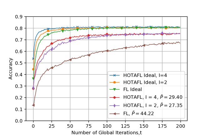
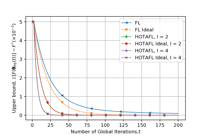
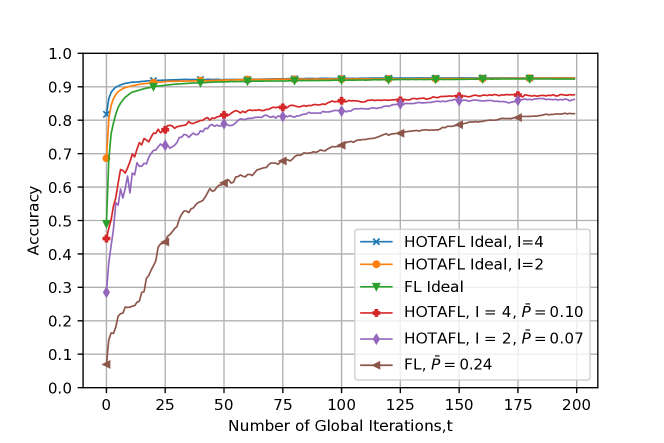
Accuracy plots are presented in Figs. 3-5, where P¯¯𝑃\bar{P} is the average transmit power. The results show that bringing the servers closer to the users enhances learning accuracy significantly. One reason for the improved performance is that the cluster structure enables the MUs share their model differences with a local server closer than the PS, reducing the adverse effects of the large-scale wireless channel effects. Another reason is that MUs receive updated models even without communicating with the PS due to local aggregations. We also observe that although more initial power is given to FL, the user updates do not reflect on the global model as much as HOTAFL does due to the effects of the wireless channel. More local iterations enables faster convergence but uses more transmit power due to the accumulating nature of IS. Even though the noise variance is high when compared to the transmit power, deploying 5MC=1005𝑀𝐶1005MC=100 receive antennas almost mitigates the noise and the interference terms [5]. Increasing τ𝜏\tau compensates the accuracy under more complex data structure. In Fig. 5, we compare the convergence rates of conventional FL and HOTAFL using the upper bound in (1), with 2N=7850,L=10,μ=1,G2=1,Γ=1,η(t)=51022105t,Pt=1+102t,β=3,𝜽PS(0)𝜽22=103formulae-sequence2𝑁7850formulae-sequence𝐿10formulae-sequence𝜇1formulae-sequencesuperscript𝐺21formulae-sequenceΓ1formulae-sequence𝜂𝑡5superscript1022superscript105𝑡formulae-sequencesubscript𝑃𝑡1superscript102𝑡formulae-sequence𝛽3superscriptsubscriptnormsubscript𝜽𝑃𝑆0superscript𝜽22superscript1032N=7850,L=10,\mu=1,G^{2}=1,\Gamma=1,\eta(t)=5\!\cdot\!10^{-2}\!-\!2\cdot 10^{-5}t,P_{t}=1+10^{-2}t,\beta=3,\left\|\bm{\theta}_{PS}(0)-\bm{\theta}^{*}\right\|_{2}^{2}=10^{3}. It can be seen that the convergence rate of HOTAFL is very close to that of the ideal case, and it becomes almost the same when the number of local iterations is increased.
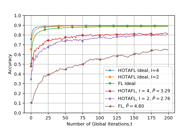
Refer to caption
Figure 2: Test accuracy for i.i.d. MNIST data with τ=1𝜏1\tau=1.
Refer to caption
Figure 3: Test accuracy for non-i.i.d. MNIST data with τ=3𝜏3\tau=3.
Refer to caption
Figure 4: Test accuracy for i.i.d. CIFAR-10 data with τ=5𝜏5\tau=5.
Refer to caption
Figure 5: Convergence rate for i.i.d. MNIST data with τ=1𝜏1\tau=1.

VI Conclusions

In this work, we have proposed HOTAFL where ISs are employed to create clusters to bring the server-side closer to the areas where MUs are more densely located. Our framework includes OTA cluster aggregations, where the MUs send their model updates to the ISs through a wireless channel with path loss and fading. We have examined the performance and convergence rate of HOTAFL through theoretical limits as well as model training where MNIST and CIFAR-10 datasets are used with both i.i.d. and non-i.i.d. data distributions. The results show that employing a cluster-based hierarchical model outperforms the conventional FL.

Appendix A

For the n𝑛n-th symbol, we have Δθ^PSn(t)=l=13Δθ^PS,ln(t)Δsuperscriptsubscript^𝜃𝑃𝑆𝑛𝑡superscriptsubscript𝑙13Δsuperscriptsubscript^𝜃𝑃𝑆𝑙𝑛𝑡\Delta\hat{\theta}_{PS}^{n}(t)=\sum_{l=1}^{3}\Delta\hat{\theta}_{PS,l}^{n}(t), so using the independence of channel coefficients, we have

𝔼[𝜽PS(t+1)𝒗(t+1)22]=𝔼[Δ𝜽^PS(t)Δ𝜽PS(t)22]𝔼delimited-[]superscriptsubscriptnormsubscript𝜽𝑃𝑆𝑡1𝒗𝑡122𝔼delimited-[]superscriptsubscriptnormΔsubscript^𝜽𝑃𝑆𝑡Δsubscript𝜽𝑃𝑆𝑡22\displaystyle\!\mathbb{E}\big{[}||\bm{\theta}_{PS}(t\!+\!1)\!-\!\bm{v}(t\!+\!1)||_{2}^{2}\big{]}=\mathbb{E}\big{[}\big{\|}\Delta\hat{\bm{\theta}}_{PS}(t)\!-\!\Delta\bm{\theta}_{PS}(t)\big{\|}_{2}^{2}\big{]}
=n=12N(𝔼[(Δθ^PS,1n(t)ΔθPSn(t))2]+l=23𝔼[(Δθ^PS,ln(t))2].\displaystyle\!\!=\!\!\sum_{n=1}^{2N}(\mathbb{E}\big{[}\!\big{(}\!\Delta\hat{\theta}_{PS,1}^{n}(t)\!-\!\Delta\theta_{PS}^{n}(t)\big{)}^{\!2}\big{]}\!\!+\!\!\sum_{l=2}^{3}\mathbb{E}\big{[}\!\big{(}\!\Delta\hat{\theta}_{PS,l}^{n}(t)\big{)}^{\!2}\big{]}\!. (29)

In the following lemmas, we will bound each of these terms.

Lemma 4.

We have

n=12N𝔼[(Δθ^PS,1n(t)ΔθPSn(t))2]superscriptsubscript𝑛12𝑁𝔼delimited-[]superscriptΔsuperscriptsubscript^𝜃𝑃𝑆1𝑛𝑡Δsuperscriptsubscript𝜃𝑃𝑆𝑛𝑡2\displaystyle\sum_{n=1}^{2N}\mathbb{E}\big{[}\big{(}\Delta\hat{\theta}_{PS,1}^{n}(t)-\Delta\theta_{PS}^{n}(t)\big{)}^{2}\big{]}
=1M2C2m1=1Mc1=1Ci1=1I(βm1,c12Kβc12¯𝔼[Δ𝜽m1,c1i1(t)22].\displaystyle=\frac{1}{M^{2}C^{2}}\sum_{m_{1}=1}^{M}\sum_{c_{1}=1}^{C}\sum_{i_{1}=1}^{I}\Big{(}\frac{\beta_{m_{1},c_{1}}^{2}}{K\bar{\beta_{c_{1}}^{2}}}\mathbb{E}\big{[}\big{\|}\Delta\bm{\theta}_{m_{1},c_{1}}^{i_{1}}(t)\big{\|}_{2}^{2}\big{]}\big{.}
.+(m2=1Mc2=1Ci2=1In=12NA1𝔼[Δθm1,c1i1,n(t)Δθm2,c2i2,n(t)])),\displaystyle\big{.}+\!\Big{(}\sum_{m_{2}=1}^{M}\!\sum_{c_{2}=1}^{C}\!\sum_{i_{2}=1}^{I}\!\sum_{n=1}^{2N}\!A_{1}\mathbb{E}\big{[}\Delta\theta_{m_{1},c_{1}}^{i_{1},n}(t)\Delta\theta_{m_{2},c_{2}}^{i_{2},n}(t)\big{]}\!\Big{)}\!\Big{)}, (30)

where A1=1βm1,c1β¯c1βm2,c2β¯c2+βm1,c1βm2,c2β¯c1β¯c2subscript𝐴11subscript𝛽subscript𝑚1subscript𝑐1subscript¯𝛽subscript𝑐1subscript𝛽subscript𝑚2subscript𝑐2subscript¯𝛽subscript𝑐2subscript𝛽subscript𝑚1subscript𝑐1subscript𝛽subscript𝑚2subscript𝑐2subscript¯𝛽subscript𝑐1subscript¯𝛽subscript𝑐2A_{1}=1-\frac{\beta_{m_{1},c_{1}}}{\bar{\beta}_{c_{1}}}-\frac{\beta_{m_{2},c_{2}}}{\bar{\beta}_{c_{2}}}+\frac{\beta_{m_{1},c_{1}}\beta_{m_{2},c_{2}}}{\bar{\beta}_{c_{1}}\bar{\beta}_{c_{2}}}

Proof:

Using (7) and (12), we have

𝔼[(Δθ^PS,1n(t)ΔθPSn(t))2]𝔼delimited-[]superscriptΔsuperscriptsubscript^𝜃𝑃𝑆1𝑛𝑡Δsuperscriptsubscript𝜃𝑃𝑆𝑛𝑡2\displaystyle\mathbb{E}\big{[}\big{(}\Delta\hat{\theta}_{PS,1}^{n}(t)-\Delta\theta_{PS}^{n}(t)\big{)}^{2}\big{]}
=𝔼[1M2C2m1=1Mm2=1Mc1=1Cc2=1Ci1=1Ii2=1IΔθm1,c1i1,n(t).\displaystyle=\mathbb{E}\Big{[}\frac{1}{M^{2}C^{2}}\sum_{m_{1}=1}^{M}\sum_{m_{2}=1}^{M}\sum_{c_{1}=1}^{C}\sum_{c_{2}=1}^{C}\sum_{i_{1}=1}^{I}\sum_{i_{2}=1}^{I}\Delta\theta_{m_{1},c_{1}}^{i_{1},n}(t)\Big{.}
.×Δθm2,c2i2,n(t)(11Kσh2β¯c1k1=1K|hm1,c1,k1i1,n(t)|2..\displaystyle\quad\Big{.}\times\Delta\theta_{m_{2},c_{2}}^{i_{2},n}(t)\Big{(}1-\frac{1}{K\sigma_{h}^{2}\bar{\beta}_{c_{1}}}\sum_{k_{1}=1}^{K}|h_{m_{1},c_{1},k_{1}}^{i_{1},n}(t)|^{2}\Big{.}\Big{.}
..1Kσh2β¯c2k2=1K|hm2,c2,k2i2,n(t)|2..\displaystyle\quad\Big{.}\Big{.}-\frac{1}{K\sigma_{h}^{2}\bar{\beta}_{c_{2}}}\sum_{k_{2}=1}^{K}|h_{m_{2},c_{2},k_{2}}^{i_{2},n}(t)|^{2}\Big{.}\Big{.}
..+1K2σh4β¯c12k1=1Kk2=1K|hm1,c1,k1i1,n(t)|2|hm2,c2,k2i2,n(t)|2)].\displaystyle\quad\Big{.}\Big{.}+\!\frac{1}{K^{2}\sigma_{h}^{4}\bar{\beta}_{c_{1}}^{2}}\!\!\sum_{k_{1}=1}^{K}\!\sum_{k_{2}=1}^{K}\!\!|h_{m_{1},c_{1},k_{1}}^{i_{1},n}\!(t)|^{2}|h_{m_{2},c_{2},k_{2}}^{i_{2},n}\!(t)|^{2}\!\Big{)}\!\Big{]}\!. (31)

Summing over all the symbols and using the independence of channel coefficients result in (30). ∎

Lemma 5.

We have

n=12N𝔼[(Δθ^PS,2n(t))2]superscriptsubscript𝑛12𝑁𝔼delimited-[]superscriptΔsuperscriptsubscript^𝜃𝑃𝑆2𝑛𝑡2\displaystyle\sum_{n=1}^{2N}\mathbb{E}\big{[}\big{(}\Delta\hat{\theta}_{PS,2}^{n}(t)\big{)}^{2}\big{]}
=m=1Mm=1mmMc=1Ci=1Iβm,cβm,cM2C2Kβ¯c2𝔼[Δ𝜽m,ci(t)22].absentsuperscriptsubscript𝑚1𝑀superscriptsubscriptsuperscript𝑚1superscript𝑚𝑚𝑀superscriptsubscript𝑐1𝐶superscriptsubscript𝑖1𝐼subscript𝛽𝑚𝑐subscript𝛽superscript𝑚𝑐superscript𝑀2superscript𝐶2𝐾superscriptsubscript¯𝛽𝑐2𝔼delimited-[]superscriptsubscriptnormΔsuperscriptsubscript𝜽superscript𝑚𝑐𝑖𝑡22\displaystyle=\sum_{m=1}^{M}\sum_{\begin{subarray}{c}m^{\prime}=1\\ m^{\prime}\neq m\end{subarray}}^{M}\!\sum_{c=1}^{C}\sum_{i=1}^{I}\frac{\beta_{m,c}\beta_{m^{\prime},c}}{M^{2}C^{2}K\bar{\beta}_{c}^{2}}\mathbb{E}\big{[}\left\|\Delta\bm{\theta}_{m^{\prime},c}^{i}(t)\right\|_{2}^{2}\big{]}. (32)
Proof:

For 1nN1𝑛𝑁1\leq n\leq N, using the independence of channel coefficients, we have

𝔼[(Δθ^PS,2n(t))2]=𝔼[(m=1Mm=1mmMc=1Ci=1I1MCKσh2β¯c..\displaystyle\mathbb{E}\big{[}\big{(}\Delta\hat{\theta}_{PS,2}^{n}(t)\big{)}^{2}\big{]}=\mathbb{E}\Big{[}\Big{(}\sum_{m=1}^{M}\sum_{\begin{subarray}{c}m^{\prime}=1\\ m^{\prime}\neq m\end{subarray}}^{M}\sum_{c=1}^{C}\sum_{i=1}^{I}\frac{1}{MCK\sigma_{h}^{2}\bar{\beta}_{c}}\Big{.}\Big{.}
..×k=1KRe{(hm,c,ki,n(t))hm,c,ki,n(t)Δθm,ci,n(t)})2]\displaystyle\hskip 14.22636pt\Big{.}\Big{.}\times\sum_{k=1}^{K}\operatorname{Re}\big{\{}\big{(}h_{m,c,k}^{i,n}(t)\big{)}^{*}h_{m^{\prime},c,k}^{i,n}(t)\Delta\theta_{m^{\prime},c}^{i,n}(t)\big{\}}\Big{)}^{2}\Big{]}
=𝔼[m=1Mm=1mmMc=1Ci=1Iβm,cβm,c2M2C2Kβ¯c2.\displaystyle=\mathbb{E}\Big{[}\sum_{m=1}^{M}\sum_{\begin{subarray}{c}m^{\prime}=1\\ m^{\prime}\neq m\end{subarray}}^{M}\sum_{c=1}^{C}\sum_{i=1}^{I}\frac{\beta_{m,c}\beta_{m^{\prime},c}}{2M^{2}C^{2}K\bar{\beta}_{c}^{2}}\Big{.}
.×((Δθm,ci,n(t))2+(Δθm,ci,n+N(t))2+Δθm,ci,n(t)Δθm,ci,n(t)..\displaystyle\enskip\Big{.}\times\big{(}\big{(}\Delta\theta_{m^{\prime},c}^{i,n}(t)\big{)}^{2}+\big{(}\Delta\theta_{m^{\prime},c}^{i,n+N}(t)\big{)}^{2}+\Delta\theta_{m,c}^{i,n}(t)\Delta\theta_{m^{\prime},c}^{i,n}(t)\big{.}\Big{.}
.Δθm,ci,n+N(t)Δθm,ci,n+N(t))]\displaystyle\hskip 85.35826pt\Big{.}\left.-\Delta\theta_{m,c}^{i,n+N}(t)\Delta\theta_{m^{\prime},c}^{i,n+N}(t)\right)\Big{]} (33)

Obtaining the expressions for N+1n2N𝑁1𝑛2𝑁N+1\leq n\leq 2N in a similar manner and combining the two, results in (32). ∎

Lemma 6.
n=12N𝔼[(Δθ^PS,3n(t))2]=σz2INPt2M2C2Kσh2m=1Mc=1Cβm,cβ¯c2.superscriptsubscript𝑛12𝑁𝔼delimited-[]superscriptΔsuperscriptsubscript^𝜃𝑃𝑆3𝑛𝑡2superscriptsubscript𝜎𝑧2𝐼𝑁superscriptsubscript𝑃𝑡2superscript𝑀2superscript𝐶2𝐾superscriptsubscript𝜎2superscriptsubscript𝑚1𝑀superscriptsubscript𝑐1𝐶subscript𝛽𝑚𝑐superscriptsubscript¯𝛽𝑐2\displaystyle\sum_{n=1}^{2N}\!\mathbb{E}\big{[}\big{(}\Delta\hat{\theta}_{PS,3}^{n}(t)\big{)}^{2}\big{]}\!=\!\frac{\sigma_{z}^{2}IN}{P_{t}^{2}M^{2}C^{2}K\sigma_{h}^{2}}\!\sum_{m=1}^{M}\!\sum_{c=1}^{C}\!\frac{\beta_{m,c}}{\bar{\beta}_{c}^{2}}. (34)
Proof:

Using the independence of channel coefficients, for 1nN1𝑛𝑁1\leq n\leq N, we have

𝔼[(Δθ^PS,3n(t))2]=𝔼[(m=1Mc=1Ci=1Ik=1K1PtMCKσh2β¯c..\displaystyle\mathbb{E}\big{[}\big{(}\Delta\hat{\theta}_{PS,3}^{n}(t)\big{)}^{2}\big{]}=\mathbb{E}\Big{[}\Big{(}\sum_{m=1}^{M}\sum_{c=1}^{C}\sum_{i=1}^{I}\sum_{k=1}^{K}\frac{1}{P_{t}MCK\sigma_{h}^{2}\bar{\beta}_{c}}\Big{.}\Big{.}
..×Re{(hm,c,ki,n(t))zc,ki,n(t)})2]\displaystyle\hskip 28.45274pt\Big{.}\Big{.}\times\operatorname{Re}\big{\{}\big{(}h_{m,c,k}^{i,n}(t)\big{)}^{*}z_{c,k}^{i,n}(t)\big{\}}\Big{)}^{2}\Big{]}
=𝔼[m=1Mc=1Ci=1Ik=1K1Pt2M2C2K2σh4β¯c2.\displaystyle=\mathbb{E}\Big{[}\sum_{m=1}^{M}\sum_{c=1}^{C}\sum_{i=1}^{I}\sum_{k=1}^{K}\frac{1}{P_{t}^{2}M^{2}C^{2}K^{2}\sigma_{h}^{4}\bar{\beta}_{c}^{2}}\Big{.}
.×(Re{(hm,c,ki,n(t))zc,ki,n(t)})2]\displaystyle\Big{.}\hskip 28.45274pt\times\big{(}\operatorname{Re}\big{\{}\big{(}h_{m,c,k}^{i,n}(t)\big{)}^{*}z_{c,k}^{i,n}(t)\big{\}}\big{)}^{2}\Big{]}
=σz2I2Pt2M2C2Kσh2m=1Mc=1Cβm,cβ¯c2.absentsuperscriptsubscript𝜎𝑧2𝐼2superscriptsubscript𝑃𝑡2superscript𝑀2superscript𝐶2𝐾superscriptsubscript𝜎2superscriptsubscript𝑚1𝑀superscriptsubscript𝑐1𝐶subscript𝛽𝑚𝑐superscriptsubscript¯𝛽𝑐2\displaystyle=\frac{\sigma_{z}^{2}I}{2P_{t}^{2}M^{2}C^{2}K\sigma_{h}^{2}}\sum_{m=1}^{M}\sum_{c=1}^{C}\frac{\beta_{m,c}}{\bar{\beta}_{c}^{2}}. (35)

The same result holds for N+1n2N𝑁1𝑛2𝑁N+1\leq n\leq 2N. Combining the two results concludes the lemma. ∎

Combining the results in Lemmas 4, 5, and 6 and applying Assumption 2 with (19) completes the proof of Lemma 1.

References

  • [1] W. Y. B. Lim, N. C. Luong, D. T. Hoang, Y. Jiao, Y. C. Liang, Q. Yang, D. Niyato, and C. Miao, “Federated learning in mobile edge networks: A comprehensive survey,” IEEE Commun. Surveys Tuts., vol. 22, no. 3, pp. 2031–2063, 2020.
  • [2] B. McMahan, E. Moore, D. Ramage, S. Hampson, and B. A. y. Arcas, “Communication-Efficient Learning of Deep Networks from Decentralized Data,” Proceedings of the 20th International Conference on Artificial Intelligence and Statistics (AISTATS), pp. 1273–1282, 2017.
  • [3] D. Gunduz, D. B. Kurka, M. Jankowski, M. M. Amiri, E. Ozfatura, and S. Sreekumar, “Communicate to earn at the edge,” IEEE Commun. Mag., vol. 58, no. 12, pp. 14–19, 2020.
  • [4] M. Mohammadi Amiri and D. Gunduz, “Machine learning at the wireless edge: Distributed stochastic gradient descent over-the-air,” IEEE Trans. Signal Process., vol. 68, pp. 2155–2169, 2020.
  • [5] M. M. Amiri, T. M. Duman, D. Gunduz, S. R. Kulkarni, and H. V. P. Poor, “Blind federated edge learning,” IEEE Trans. Wireless Commun., vol. 20, no. 8, pp. 5129–5143, 2021.
  • [6] M. M. Amiri, S. R. Kulkarni, and H. V. Poor, “Federated learning with downlink device selection,” arXiv preprint arXiv:2107.03510, 2021.
  • [7] G. Zhu, Y. Wang, and K. Huang, “Broadband analog aggregation for low-latency federated edge learning,” IEEE Trans. Wireless Commun., vol. 19, no. 1, pp. 491–506, 2020.
  • [8] G. Zhu, Y. Du, D. Gündüz, and K. Huang, “One-bit over-the-air aggregation for communication-efficient federated edge learning: Design and convergence analysis,” IEEE Trans. Wireless Commun., vol. 20, no. 3, pp. 2120–2135, 2021.
  • [9] M. Chen, N. Shlezinger, H. V. Poor, Y. C. Eldar, and S. Cui, “Communication-efficient federated learning,” Proceedings of the National Academy of Sciences, vol. 118, no. 17, 2021.
  • [10] B. Tegin and T. M. Duman, “Blind federated learning at the wireless edge with low-resolution adc and dac,” IEEE Trans. on Wireless Commun., 2021.
  • [11] ——, “Federated learning over time-varying channels,” in IEEE Global Communications Conference (GLOBECOM), Madrid, Spain, Dec. 2021.
  • [12] T. Sery, N. Shlezinger, K. Cohen, and Y. Eldar, “Over-the-air federated learning from heterogeneous data,” IEEE Trans. Signal Process., vol. 69, pp. 3796–3811, 2021.
  • [13] C. T. Dinh, N. H. Tran, M. N. Nguyen, C. S. Hong, W. Bao, A. Y. Zomaya, and V. Gramoli, “Federated learning over wireless networks: Convergence analysis and resource allocation,” IEEE/ACM Transactions on Networking, vol. 29, no. 1, pp. 398–409, 2020.
  • [14] D. Liu and O. Simeone, “Privacy for free: Wireless federated learning via uncoded transmission with adaptive power control,” IEEE J. Sel. Areas Commun., vol. 39, no. 1, pp. 170–185, 2021.
  • [15] M. M. Amiri, D. Gunduz, S. R. Kulkarni, and H. Vincent Poor, “Convergence of federated learning over a noisy downlink,” IEEE Trans. Wireless Commun., pp. 1–16, 2021.
  • [16] M. S. H. Abad, E. Ozfatura, D. Gunduz, and O. Ercetin, “Hierarchical federated learning across heterogeneous cellular networks,” in ICASSP 2020-2020 IEEE International Conference on Acoustics, Speech and Signal Processing (ICASSP).   IEEE, 2020, pp. 8866–8870.
  • [17] L. Liu, J. Zhang, S. Song, and K. B. Letaief, “Client-edge-cloud hierarchical federated learning,” in ICC 2020-2020 IEEE International Conference on Communications (ICC).   IEEE, 2020, pp. 1–6.
  • [18] S. Luo, X. Chen, Q. Wu, Z. Zhou, and S. Yu, “HFEL: Joint edge association and resource allocation for cost-efficient hierarchical federated edge learning,” IEEE Trans. Wireless Commun., vol. 19, no. 10, pp. 6535–6548, 2020.
  • [19] J. Wang, S. Wang, R.-R. Chen, and M. Ji, “Local averaging helps: Hierarchical federated learning and convergence analysis,” arXiv preprint arXiv:2010.12998, 2020.
  • [20] C. Briggs, Z. Fan, and P. Andras, “Federated learning with hierarchical clustering of local updates to improve training on non-iid data,” in 2020 International Joint Conference on Neural Networks (IJCNN).   IEEE, 2020, pp. 1–9.
  • [21] Y. LeCun, “The MNIST database of handwritten digits,” http://yann. lecun. com/exdb/mnist/, 1998.
  • [22] A. Krizhevsky et al., “Learning multiple layers of features from tiny images,” 2009.
  • [23] D. P. Kingma and J. Ba, “Adam: A method for stochastic optimization,” arXiv preprint arXiv:1412.6980, 2014.