Data Blurring – Possible extensions and explorations

1 Coverage guarantees for fixed-design GLMs

Fahrmeir-style intervals seem to work fine empirically for logistic regression but mildly violate FCR control for Poisson regression when using data fission. For data splitting, they seem to violate FCR control.

In general, these intervals tend to be fairly similar in size as n grows, as we can seen in Figure 1.

Figure 1: Average size of standard errors as a function of number of data points

1.1 Empirical Results (Poisson Regression)

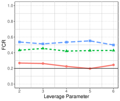
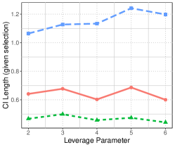
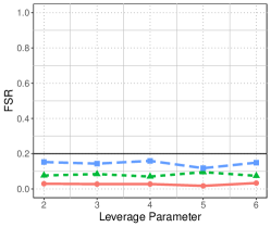
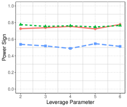
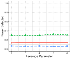
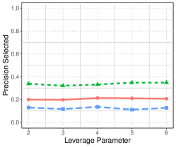
Figure 2: Fahrmeir Intervals Low n, one highly influential point

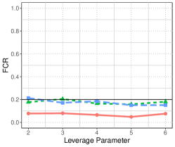
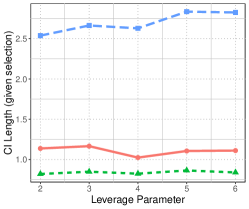
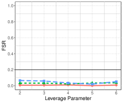
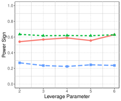
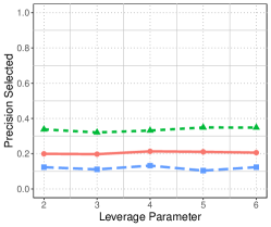
Figure 3: Sandwich Intervals from ClubSandwich package Low n, one highly influential point

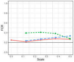
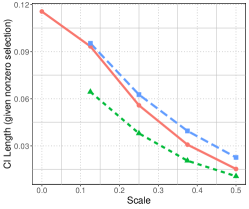
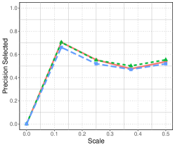
Figure 4: Fahrmeir Intervals Varying signal strength, large $n$ = 500

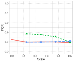
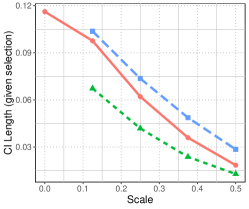
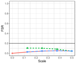
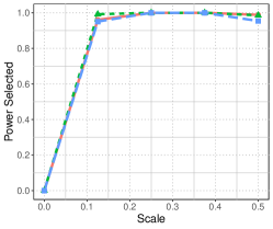
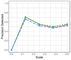
Figure 5: Sandwich Intervals from ClubSandwich package Varying signal strength, large $n$ = 500

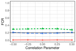
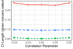
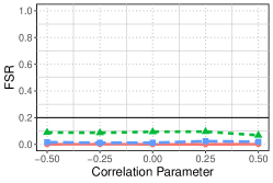
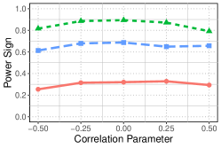
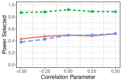
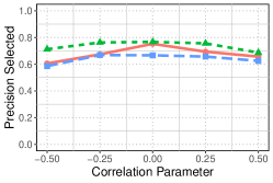
Figure 6: Fahrmeir Intervals Varying correlation strength of features, large $n$ = 500

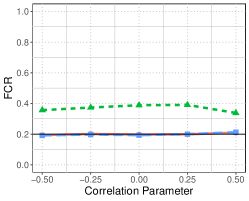
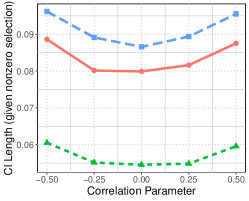
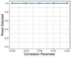
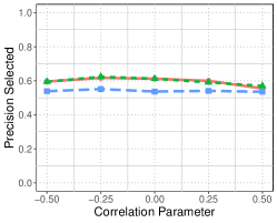
Figure 7: Sandwich Intervals from ClubSandwich package Varying correlation strength of features, large $n$ = 500

1.2 Empirical Results (Logistic)

Figure 9: FCR, CI width, FSR, power for the sign of parameters, and power and precision for the selected features, when varying the signal strength $S_{\Delta}$ in $\{0,0.1,0.2,0.3,0.4,0.5\}$. The hyperparameter $p$ is chosen as $0.2$ and target FCR for confidence intervals is set at $0.2$. We note that data fission offers smaller confidence interval widths when compared to both data splitting and the (invalid) approach that reuses the full dataset for both selection and inference.

Figure 11: ClubSandiwch variant. FCR, CI width, FSR, power for the sign of parameters, and power and precision for the selected features, when varying the signal strength $S_{\Delta}$ in $\{0,0.1,0.2,0.3,0.4,0.5\}$. The hyperparameter $p$ is chosen as $0.2$ and target FCR for confidence intervals is set at $0.2$. We note that data fission offers smaller confidence interval widths when compared to both data splitting and the (invalid) approach that reuses the full dataset for both selection and inference.

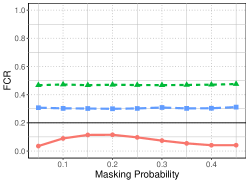
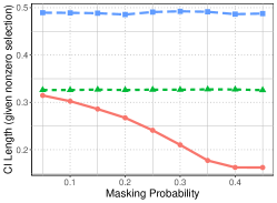
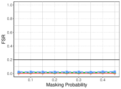
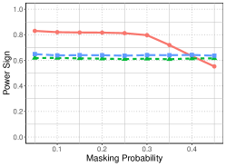
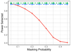
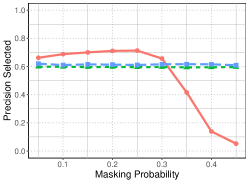
Figure 12: FCR, CI width, power for the sign of parameters, and power/precision for the selected features, when varying the hyperparameter $p$ in $\{0.05,0.1,0.15,0.2,0.25,0.3,0.35,0.4,0.45\}$ with fixed signal strength $S_{\Delta}=0.5$. The power and precision are higher when $p$ is closer to either $0$ or $1$ rather than $0.5$. Interestingly, however, the confidence interval lengths only slightly increases as $p$ varies away from $0.5$.

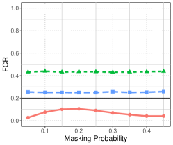
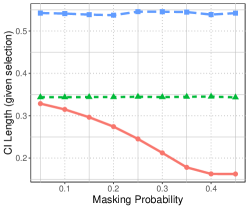
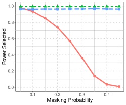
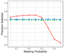
Figure 13: clubSandwich variant. FCR, CI width, power for the sign of parameters, and power/precision for the selected features, when varying the hyperparameter $p$ in $\{0.05,0.1,0.15,0.2,0.25,0.3,0.35,0.4,0.45\}$ with fixed signal strength $S_{\Delta}=0.5$. The power and precision are higher when $p$ is closer to either $0$ or $1$ rather than $0.5$. Interestingly, however, the confidence interval lengths only slightly increases as $p$ varies away from $0.5$.

2 Proof

LABEL:thm:glm_clt_est demonstrates that $\hat{\beta}_{n}(M)\overset{p}{\rightarrow}\beta^{\star}_{n}(M)$. Due to the assumption that the quasi-likelihood function is twice continuously differentiable, $H_{n}$ and $s_{n}$ are both continuous function with respect to $\beta$, so by the continuous mapping theorem, $\hat{H}_{n}\overset{p}{\rightarrow}H_{n}(\beta^{\star}_{n}(M))$ and $s_{n}(\hat{\beta}_{n}(M))\overset{p}{\rightarrow}s_{n}(\beta^{\star}_{n}(M))$. In the rest of the argument, we drop the explicit dependence on the selected model ($M$) to avoid clunky notation so let $\beta^{\star}_{n}:=\beta^{\star}_{n}(M)$ and $x_{i\cdot M}:=x_{i}$ in what follows. Now, note that

$$\mathbb{E}[s_{n}(\beta^{\star}_{n})s_{n}(\beta^{\star}_{n})^{T}] =\text{Var}\left(s_{n}(\beta^{\star}_{n})\right)+\mathbb{E}[s_{n}(\beta^{\star}_{n})]\mathbb{E}[s_{n}(\beta^{\star}_{n})]]^{T}$$

$$=V_{n}\left(\beta^{\star}_{n}\right)+\sum_{i=1}^{n}x_{i}\left(g(y_{i})-m_{i}\right)^{2}v_{i}^{-2}\left(\frac{\partial m_{i}}{\partial\eta_{i}}\right)^{2}x_{i}^{T},$$

where the last term is positive semidefinite since it is a Gram matrix.

Recall that if two matrices $A,B$ are positive semidefinite then: (i) $A^{-1}$ is positive semidefinite, (ii) $A+B$ is positive semidefinite, (iii) ABA is positive semidefnite. Therefore since $H_{n}\left(\beta^{\star}_{n}\right)$ is also positive semi definite by assumption, we know that

$$H^{-1}_{n}\left(\beta^{\star}_{n}\right)\left(\mathbb{E}[s_{n}(\beta^{\star}_{n})s_{n}(\beta^{\star}_{n})^{T}]-V_{n}\left(\beta^{\star}_{n}\right)\right)H^{-1}_{n}\left(\beta^{\star}_{n}\right)$$

is positive semidefnite. Denote the Cholesky decomposition of $H^{-1}_{n}\left(\beta^{\star}_{n}\right)\mathbb{E}[s_{n}(\beta^{\star}_{n})s_{n}(\beta^{\star}_{n})^{T}]H^{-1}_{n}\left(\beta^{\star}_{n}\right)$ as $LL^{T}$ and the Cholesky decomposition of $H^{-1}_{n}\left(\beta^{\star}_{n}\right)V_{n}\left(\beta^{\star}_{n}\right)H^{-1}_{n}\left(\beta^{\star}_{n}\right)$ as $MM^{T}$. From the above, we knot that $LL^{T}-MM^{T}$ is psd which implies that

$$L_{kk}-M_{kk}=\sqrt{[H^{-1}_{n}\left(\beta^{\star}_{n}\right)\mathbb{E}[s_{n}(\beta^{\star}_{n})s_{n}(\beta^{\star}_{n})^{T}]H^{-1}_{n}\left(\beta^{\star}_{n}\right)]_{kk}}-\sqrt{[H^{-1}_{n}\left(\beta^{\star}_{n}\right)V_{n}\left(\beta^{\star}_{n}\right)H^{-1}_{n}\left(\beta^{\star}_{n}\right)]_{kk}}\geq 0$$

since the diagonal entries must be positive.

By the WLLN, $\hat{V}_{n}\overset{p}{\rightarrow}\mathbb{E}[s_{n}(\beta^{\star}_{n})s_{n}(\beta^{\star}_{n})^{T}]$ which combined with the above statement shows us

$$\lim_{n\rightarrow\infty}P\left(\sqrt{[\hat{H}_{n}^{-1}\hat{V}_{n}^{1}\hat{H}_{n}^{-1}]_{kk}}\geq\sqrt{[\hat{H}_{n}^{-1}\left(\beta^{\star}_{n}\right)V_{n}\left(\beta^{\star}_{n}\right)\hat{H}_{n}^{-1}\left(\beta^{\star}_{n}\right)]_{kk}}\right)=1.$$ (1)

Appealing again to LABEL:thm:glm_clt_est, we have that:

$$1-\alpha =\lim_{n\rightarrow\infty}P\left([\beta_{n}^{\star}]_{k}\in\left[[\hat{\beta}_{n}]_{k}\pm z_{\alpha/2}M_{kk}\right]\right)$$

$$\leq\lim_{n\rightarrow\infty}P\left([\beta_{n}^{\star}]_{k}\in\left[[\hat{\beta}_{n}]_{k}\pm z_{\alpha/2}[\hat{H}_{n}^{-1}\hat{V}_{n}^{1/2}]_{kk}\right]\right),$$

where the first line follows from standard arguments and the second line follows from Equation 1. This concludes the proof.

3 Fixed Projections

Let $Y\sim N(\mu,\Sigma)$ with $\mu\in\mathbb{R}^{n}$ and $\Sigma\in\mathbb{R}^{n\times n}$. Consider some fixed matrix $A\in\mathbb{R}^{m\times n}$. We wish to conduct inference on the distribution of $Y|AX$.

Fact 1 (Affine property of Gaussian distribution).

Let $Y\sim N(\mu,\Sigma)$ and $A\in\mathbb{R}^{m\times n}$. Then

$$AY\sim N(A\mu,A\Sigma A^{T})$$

Fact 2 (Conditioning on Gaussian regression ).

If $Y\sim N(\mu,\Sigma)$ is partitioned as follows

$$\mathbf{Y}=\left[\begin{array}[]{l}\mathbf{Y}_{1}\\ \mathbf{Y}_{2}\end{array}\right]\text{ with sizes }\left[\begin{array}[]{c}q\times 1\\ (N-q)\times 1\end{array}\right]$$

and accordingly $\bm{\mu}$ and $\bm{\Sigma}$ are partitioned as follows

$$\bm{\mu} =\left[\begin{array}[]{l}\bm{\mu}_{1}\\ \bm{\mu}_{2}\end{array}\right]\text{ with sizes }\left[\begin{array}[]{c}q\times 1\\ (N-q)\times 1\end{array}\right]$$

$$\bm{\Sigma} =\left[\begin{array}[]{ll}\bm{\Sigma}_{11}&\bm{\Sigma}_{12}\\ \bm{\Sigma}_{21}&\bm{\Sigma}_{22}\end{array}\right]\text{ with sizes }\left[\begin{array}[]{cc}q\times q&q\times(N-q)\\ (N-q)\times q&(N-q)\times(N-q)\end{array}\right]$$

then the distribution of $\mathbf{X}_{1}$ conditional on $\mathbf{Y}_{2}=\mathbf{a}$ is multivariate normal $\left(\mathbf{x}_{1}\mid\mathbf{x}_{2}=\mathbf{a}\right)\sim N(\overline{\bm{\mu}},\overline{\bm{\Sigma}})$ where

$$\overline{\bm{\mu}}=\bm{\mu}_{1}+\bm{\Sigma}_{12}\bm{\Sigma}_{22}^{-1}\left(\mathbf{a}-\bm{\mu}_{2}\right)$$

and covariance matrix

$$\overline{\bm{\Sigma}}=\bm{\Sigma}_{11}-\bm{\Sigma}_{12}\bm{\Sigma}_{22}^{-1}\bm{\Sigma}_{21}$$

To apply the above two facts to the problem define a new matrix $A_{0}=\left[\begin{array}[]{l}I_{n}\\ A\end{array}\right]$ and apply the above formulas. If we make the simplifying assumption that $\Sigma=\sigma^{2}I_{n}$, we have that

$$A_{0}Y\sim N\left(\left[\begin{array}[]{l}\mu\\ A\mu\end{array}\right],\sigma^{2}\left[\begin{array}[]{ll}I&A^{T}\\ A&AA^{T}\\ \end{array}\right]\right)$$

Therefore,

$$Y|AY\sim N\left(\mu+A^{T}(AA^{T})^{-1}(AY-A\mu),\sigma^{2}\left(I-A^{T}(AA^{T})^{-1}A\right)\right)$$

Remark 1.

Data splitting can be considered as a special example of this where you choose a collection of indices to allocate to selection $D_{\text{sel}}\subseteq[n]$ and consider the distribution of $Y|\{Y_{i}:i\in D_{\text{sel}}\}$. In this case, we would let $A$ be the concatenated matrix with each row $A_{i}=e_{j}^{T}$ for each $j\in D_{\text{sel}}$. We would have

$$Y|\{Y_{i}:i\in D_{\text{sel}}\}\sim N(\alpha\mu+(1-\alpha)Y,\sigma^{2}\text{diag}\left(\alpha)\right)$$

where $\alpha\in\mathbb{R}^{n}$ with

$$\alpha_{i}=\begin{cases}1\text{ whenever }i\not\in D_{\text{sel}}\\ 0\text{ whenever }i\in D_{\text{sel}}\end{cases}$$

3.1 Alternative way of splitting Fisher information

Suppose we have a “target” covariance matrix for $AY$ we wish to obtain $\sigma^{2}T$ where $T$ is any symmetric and positive semidefinite matrix of the analyst’s choice. Simply take the eigendecomposition of $T=Q\Delta Q^{T}$ and set

$$A=Q\Delta^{1/2}.$$

This allows you to choose any covariance matrix for the selection stage that they wish — but this also forces the analyst to pay a price at the inference stage with lower information. Note the decomposition for Fisher information Using the chain rule for Fisher information, we have that

$$E[\mathcal{I}_{Y|AY}(\mu)]=\mathcal{I}_{Y}(\mu)-\mathcal{I}_{AY}(\mu).$$

So higher Fisher information in the selection stage necessitates lower information in the inference stage.

4 Extensions to Unknown Variance

4.1 Preliminaries

For simplicity, throughout this document we assume that $\Sigma=\sigma^{2}I_{n}$. As before, we assume that $y_{i}$ is the dependent variable and $x_{i}\in\mathbb{R}^{p}$ is a vector of $p$ features for $i=1,\ldots,n$ samples. We also denote $X=(x_{1},...,x_{n})^{T}$ as the model design matrix and $Y=(y_{1},...,y_{n})^{T}$ with the following structural equation:

$$Y=\mu+\epsilon\text{ with }\epsilon=(\epsilon_{1},...,\epsilon_{n})^{T}\sim N(0,\sigma^{2}I_{n}),$$

Note the following important facts:

1. In a fixed-$X$ setting, if $n>p$, then taking $\hat{\sigma}^{2}$ to be the variance estimated from the residuals by fitting the full model with all $p$ covariates is a consistent estimate of $\sigma^{2}$. See section 5.3 of selective_inference_asymptotics

2. In a fixed-$X$ setting, if $p>n$ then $\sigma^{2}=\frac{1}{n-1}\sum_{i=1}^{n}(Y_{i}-\bar{Y})^{2}$ is an overestimate of $\sigma^{2}$. See section 2.3 of uniform_asymptotic.

4.2 Approach 1: Estimate variance after data blurring

Suppose the true variance is $\sigma^{2}$ but because it is unknown, we blur with $Z\sim N(0,\sigma_{0}^{2})$.As usual, we let $f(Y)=Y+\tau Z$ and $g(Y)=Y-\frac{1}{\tau}Z$

We then have that

$$(f(Y),g(Y))^{T}\sim N\left(\mu,\begin{pmatrix}(\sigma^{2}+\sigma_{0}^{2}\tau^{2})I_{n}&(\sigma^{2}-\sigma_{0}^{2})I_{n}\\ (\sigma^{2}-\sigma_{0}^{2})I_{n}&(\sigma^{2}+\frac{\sigma_{0}^{2}}{\tau^{2}})I_{n}\end{pmatrix}\right).$$

By standard properties of a multivariate Gaussian, we have that,

$$g(Y)|f(Y)\sim N\left(\mu+(f(Y)-\mu)\frac{\sigma^{2}-\sigma_{0}^{2}}{\sigma^{2}+\tau^{2}\sigma_{0}^{2}},\left(\sigma^{2}+\frac{\sigma_{0}^{2}}{\tau^{2}}+\frac{(\sigma^{2}-\sigma_{0}^{2})^{2}}{\sigma^{2}+\tau^{2}\sigma_{0}^{2}}\right)I_{n}\right).$$

Case 1: $n>p$

By the arguments discussed above, we’re assuming we have an estimator $s^{2}$ which is a consistent estimate of the variance of $g(Y)|f(Y)$. Let $f(\sigma^{2})=\sigma^{2}+\frac{\sigma_{0}^{2}}{\tau^{2}}+\frac{(\sigma^{2}-\sigma_{0}^{2})^{2}}{\sigma^{2}+\tau^{2}\sigma_{0}^{2}}$. Take $f^{-1}$ to be the non-negative solution to the quadratic equation that solves for $\sigma^{2}$ given $f(\sigma^{2})$. Then by the continuous mapping theorem, $f^{-1}(s^{2})$ will be a consistent estimate for $\sigma^{2}$. Denote $f^{-1}(s^{2})=\hat{\sigma}^{2}$

Now, we can shift and rescale the mean so it is centered properly and we get

$$\left(g(Y)(\hat{\sigma}^{2}+\tau^{2}\sigma_{0}^{2})-f(Y)(\hat{\sigma}^{2}-\sigma_{0}^{2})\right)\frac{1}{\sigma_{0}^{2}(1+\tau^{2})}|f(Y)\overset{d}{\to}N\left(\mu,\frac{\sigma^{2}+\tau^{2}\sigma_{0}^{2}}{\sigma_{0}^{2}(1+\tau^{2})}\left(\sigma^{2}+\frac{\sigma_{0}^{2}}{\tau^{2}}+\frac{(\sigma^{2}-\sigma_{0}^{2})^{2}}{\sigma^{2}+\tau^{2}\sigma_{0}^{2}}\right)I_{n}\right)$$

which then allows us to apply the same set of arguments as in the known variance case but with a messier variance term to deal with. Note: this ends up being much more messy and less clean than approach 2 in the next section, but I’m still keeping this here as a point of comparison. It also occurs to me that it might be possible to extend this argument to get a finite sample guarantee but approach 2 below relies on asymptotic arguments in a much more central way.

Case 2: $p>n$

This doesn’t appear tractable to me. If we have $s^{2}$ which is an overestimate of $\text{Var}\left(g(Y)|f(Y)\right)$, then applying the same arguments above will then give us $\hat{\sigma}^{2}=f^{-1}(s^{2})$ which is an overestimate of $\sigma^{2}$. But we need to have a consistent estimate of the bias term $(f(Y)-\mu)\frac{\sigma^{2}-\sigma_{0}^{2}}{\sigma^{2}+\tau^{2}\sigma_{0}^{2}}$ in order to get a properly centered confidence interval.

4.3 Approach 2: Estimate variance before data blurring

Case 1: $n>p$

We first fit a regression using all covariates on the non-blurred dataset Y to get a preliminary estimate $\hat{\sigma}^{2}$. From the above papers, we know $\hat{\sigma}^{2}\overset{p}{\to}\sigma^{2}$.

By Slutsky’s theorem, $\frac{Y}{\hat{\sigma}}\overset{d}{\to}N(\frac{\mu}{\sigma},I_{n})$. Draw an independent $Z\sim N(0,I_{n})$ and define $f(Y)=\frac{Y}{\hat{\sigma}}+\tau Z$ and $g(Y)=\frac{Y}{\hat{\sigma}}-\frac{1}{\tau}Z$. Applying the continuous mapping theorem to the joint density of $(\frac{Y}{\hat{\sigma}},Z)$ implies that $(f(Y),g(Y))^{T}\overset{d}{\to}N\left(\frac{\mu}{\sigma},\begin{pmatrix}(1+\tau^{2})I_{n}&0\\ 0&(1+\frac{1}{\tau^{2}})I_{n}\end{pmatrix}\right)$. Applying Slutsky’s theorem once more gives us that $(\hat{\sigma}f(Y),\hat{\sigma}g(Y))^{T}\overset{d}{\to}N\left(\mu,\begin{pmatrix}\sigma^{2}(1+\tau^{2})I_{n}&0\\ 0&\sigma^{2}(1+\frac{1}{\tau^{2}})I_{n}\end{pmatrix}\right)$.

The rest of the arguments follow exactly as in the case with known variance but now results in confidence intervals with asymptotic rather than finite sample coverage.

Case 2: $p>n$

We now have an estimator $\hat{\sigma}^{2}$ which is an overestimate of the variance. Assume $\hat{\sigma}\overset{p}{\to}\sigma_{0}$ with $\sigma_{0}>\sigma$ Apply all of the arguments given above, we now have that:

$$(\hat{\sigma}f(Y),\hat{\sigma}g(Y))^{T}\overset{d}{\to}N\left(\mu,\begin{pmatrix}(\sigma^{2}+\sigma_{0}^{2}\tau^{2})I_{n}&(\sigma^{2}-\sigma_{0}^{2})I_{n}\\ (\sigma^{2}-\sigma_{0}^{2})I_{n}&(\sigma^{2}+\frac{\sigma_{0}^{2}}{\tau^{2}})I_{n}\end{pmatrix}\right)$$

We now run into roughly the same issues as we see in approach 2 above. Conditioning on $f(Y)$ results in a bias term which requires a consistent estimate of $\hat{\sigma}^{2}$ to get rid of.