Counting Simplices in Hypergraph Streams

Abstract

We consider the problem of space-efficiently estimating the number of simplices in a hypergraph stream. This is the most natural hypergraph generalization of the highly-studied problem of estimating the number of triangles in a graph stream. Our input is a $k$-uniform hypergraph $H$ with $n$ vertices and $m$ hyperedges, each hyperedge being a $k$-sized subset of vertices. A $k$-simplex in $H$ is a subhypergraph on $k+1$ vertices $X$ such that all $k+1$ possible hyperedges among $X$ exist in $H$. The goal is to process the hyperedges of $H$, which arrive in an arbitrary order as a data stream, and compute a good estimate of $T_{k}(H)$, the number of $k$-simplices in $H$.

We design a suite of algorithms for this problem. As with triangle-counting in graphs (which is the special case $k=2$), sublinear space is achievable but only under a promise of the form $T_{k}(H)\geq T$. Under such a promise, our algorithms use at most four passes and together imply a space bound of

$$O\left(\varepsilon^{-2}\log\delta^{-1}\mathop{\text{polylog}}n\cdot\min\left\{\frac{m^{1+1/k}}{T},\frac{m}{T^{2/(k+1)}}\right\}\right)$$

for each fixed $k\geq 3$, in order to guarantee an estimate within $(1\pm\varepsilon)T_{k}(H)$ with probability at least $1-\delta$. We also give a simpler $1$-pass algorithm that achieves $O\left(\varepsilon^{-2}\log\delta^{-1}\log n\cdot(m/T)\left(\Delta_{E}+\Delta_{V}^{1-1/k}\right)\right)$ space, where $\Delta_{E}$ (respectively, $\Delta_{V}$) denotes the maximum number of $k$-simplices that share a hyperedge (respectively, a vertex), which generalizes a previous result for the $k=2$ case. We complement these algorithmic results with space lower bounds of the form $\Omega(\varepsilon^{-2})$, $\Omega(m^{1+1/k}/T)$, $\Omega(m/T^{1-1/k})$ and $\Omega(m\Delta_{V}^{1/k}/T)$ for multi-pass algorithms and $\Omega(m\Delta_{E}/T)$ for $1$-pass algorithms, which show that some of the dependencies on parameters in our upper bounds are nearly tight. Our techniques extend and generalize several different ideas previously developed for triangle counting in graphs, using appropriate innovations to handle the more complicated combinatorics of hypergraphs.

1 Introduction

Estimating the number of triangles in a massive input graph is a fundamental algorithmic problem that has attracted over two decades of intense research [AYZ97, BKS02, JG05, BFL⁺06, SV11, TKM11, KMPT12, PT12, BOV13, PTTW13, JSP15, BFKP16, MVV16, BC17, CJ17, KP17, JK21]. It is easy to see why. On the one hand, the problem arises in applications where a complex real-world network is naturally modeled as a graph and the number of triangles is a crucial statistic of the network. Such applications are found in many different domains, such as social networks [CF10, LHK10, New03], the web graph [BBCG08, WCW⁺18], and biological networks [RH03]; see [TKM11] for a more detailed discussion of such applications. On the other hand, a triangle is perhaps the most basic nontrivial pattern in a graph and as such, triangle counting is a problem with a rich theory and connections to many areas within computer science [AYZ97, ELRS15, GP18, NPRR18, DKPW20] and combinatorics [Man07, Fis89, KV04, Raz08].

In this work, we study the natural generalization of this problem to massive hypergraphs. Just as graphs model pairwise interactions between entities in a network, hypergraphs model higher arity interactions. For instance, in an academic collaboration network with researchers being the vertices, it would be natural to model coauthorships on research papers and articles using hyperedges, each of which can be incident to more than two vertices. Just as we may use triangle counts to study clustering behaviors in graphs or even in different portions of a single graph, we may analyze higher-order clustering behaviors in the $3$-uniform hypergraph $H$ formed by all three-way coauthorships by counting $3$-simplices in $H$. A $3$-simplex on four vertices $\{u,v,w,x\}$ is the structure formed by the hyperedges $\{uvw,uvx,uwx,vwx\}$: it is the natural $3$-dimensional analog of a triangle in an ordinary graph.

1.1 Our Results

We design several algorithms for space-efficiently estimating the number of $k$-simplices in a $k$-uniform hypergraph $H$ that is given as a stream of hyperedges. A $k$-simplex is a complete $k$-uniform hypergraph on $k+1$ vertices. The special case $k=2$ is the triangle counting problem which, as noted above, is intensely investigated. Indeed, even in this setting of streaming algorithms, triangle counting is highly studied, with new algorithmic techniques being developed as recently as early 2021 [JK21]. There is also a body of work on generalizing these results to the problem of estimating the number of occurrences of patterns (a.k.a. motifs) more complicated than triangles, e.g., fixed-size cliques and cycles [MMPS11, KMSS12, PTTW13, BC17, KMPV19, Vor20]. Our work adds to this literature by generalizing in a different direction: we generalize the class of inputs from graphs to hypergraphs and focus on counting the simplest nontrivial symmetric motifs, i.e., $k$-simplices.

Our algorithms provide optimal space bounds (up to log factors) in certain parameter regimes; we prove this optimality by giving a set of matching lower bounds. In certain other parameter regimes, there remains a gap between our best upper bounds and lower bounds, which immediately provides a goal for future work on this problem. Below are informal statements of our major algorithmic results.

Theorem 1 (Upper bounds; informal).

Let $H$ be an $n$-vertex $k$-uniform hypergraph, presented as a stream of $m$ hyperedges, that is promised to contain $T$ or more $k$-simplices. Suppose that each hyperedge is contained in at most $\Delta_{E}$ such simplices and each vertex is contained in at most $\Delta_{V}$ of them. Then, there are algorithms for $(1\pm\varepsilon)$-estimating $T_{k}(H)$, the number of $k$-simplices in $H$, with the following guarantees:

1. a $4$-pass algorithm using $\widetilde{O}(m^{1+1/k}/T)$ space;

2. a $2$-pass algorithm using $\widetilde{O}(m/T^{2/(k+1)})$ space, provided $k\geq 3$; and

3. a $1$-pass algorithm using $\widetilde{O}(m(\Delta_{E}+\Delta_{V}^{1-1/k})/T)$ space.

Each of these algorithms is randomized and fails with probability at most $\delta$.

Formal versions of these results appear as Theorem 4 in Section 4, Theorem 7 in Section 5.4, and Theorem 8 in Section 5.5, respectively. Along the way, we also obtain some other algorithmic results—stated as Theorem 13, Theorem 5, and Theorem 6—that we include to paint a more complete picture, even though the space complexities of those algorithms are dominated by the algorithms behind Theorem 1. In Section 2, we give a high-level overview of the techniques behind these algorithmic results. As we shall see, we take several ideas from triangle-counting algorithms as inspiration, but the “correct” way to extend these ideas to hypergraphs is far from obvious. Indeed, we shall see that some of the more “obvious” extensions lead to the less-than-best algorithms hinted at above.

Next, we informally state our lower bound results. These are not the main technical contributions of this paper, but they play the important role of clarifying where our algorithms are optimal and where there might be room for improvement. As in Theorem 1, we denote the number of $k$-simplices in $H$ by $T_{k}(H)$.

Theorem 2 (Lower bounds; informal).

Let $k,n,m,H,\Delta_{E},\Delta_{V}$ be as above. Suppose an algorithm makes $p$ passes over a stream of hyperedges of $H$, using at most $S$ bits of working memory, and distinguishes between the cases $T_{k}(H)=0$ and $T_{k}(H)\geq T$ with probability at least $2/3$. Then the following lower bounds apply.

1. With $T=1$ and $p=O(1)$, a sublinear-space solution is impossible: we must have $S=\Omega(n^{k})$.

2. With $p=1$, we must have $S=\Omega(m\Delta_{E}/T)$.

3. With $p=O(1)$, we must have $S=\Omega(m^{1+1/k}/T)$, $S=\Omega(m/T^{1-1/k})$, and $S=\Omega(m\Delta_{V}^{1/k}/T)$.

Here, a bound of the form $\Omega(Q)$ should be interpreted as ruling out the existence of an algorithm that can guarantee a space bound of $o(Q)$. If, instead, the streaming algorithm distinguishes between the cases $T_{k}(H)<(1-\varepsilon)T$ and $T_{k}(H)>(1+\varepsilon)T$, then the following lower bound applies.

1. With $p=O(1)$, we must have $S=\Omega(\varepsilon^{-2})$.

There is some definitional subtlety in the use of asymptotic notation in these lower bound results, hinted at in the language above. The picture will become clearer when we state these results formally, in Section 6.

1.2 Closely Related Previous Work

To the best of our knowledge, this is the first work to study the simplex counting problem in hypergraphs in the setting just described (the work of [KKP18] on counting general hypergraph patterns is not closely related; see Section 1.3). We now summarize some highlights of previous work on the triangle counting problem (in graphs), with a focus on streaming algorithms, so as to provide context for our contributions.

Suppose an $n$-vertex $m$-edge graph $G$ is given as a stream of edges and we wish to estimate the number of triangles, $T_{3}(G)$. It is not hard to show that, absent any promises on the structure of $G$, this problem requires $\Omega(n^{2})$ space, even with multiple passes, thus precluding a sublinear-space solution. Therefore, all work in this area seeks bounds under a promise that $T_{3}(G)\geq T$, for some nontrivial threshold $T$. Intuitively, the larger this threshold, the easier the problem, so we expect the space complexity to decrease. The earliest nontrivial streaming solution [BKS02] reduced triangle counting to a combination of $\ell_{0}$, $\ell_{1}$, and $\ell_{2}$ estimation and achieved $\widetilde{O}((mn/T)^{2})$ space by using suitable linear sketches. Almost all algorithms developed since then have instead used some sort of sampling to extract a small portion of $G$, perform some computation on this sample, and then extrapolate to estimate $T_{3}(G)$.

Over the years, a number of different sampling strategies have been developed, achieving different, sometimes incomparable, guarantees. Here is a whirlwind tour through this landscape of strategies. One could sample an edge uniformly at random (using reservoir sampling), then count common neighbors of its endpoints [JG05]; or sample an edge uniformly and sample a vertex not incident to it [BFL⁺06]; or sample a subset of edges by independently picking each with a carefully adjusted probability $p$ [KMPT12, BOV13]; or choose a random color for each vertex and collect all monochromatic edges [PT12]; or sample a subset of vertices at random and collect all edges incident to the sample [BOV13]. One could collect two random subsets of vertices at different sampling rates and further sample edges between the two subsets [KP17]; or, as in a very recent algorithm, sample a subset of vertices at rate $p$ and further sample edges incident to this sample at rate $q$, for well-chosen $p$ and $q$ [JK21]. Notice that in the just-mentioned algorithms, the sampling technique decides whether or not to store an edge without regard to other edges that may be in store and is thus not actively trying to “grow” a triangle around a sampled edge. We shall call such sampling strategies oblivious.

Besides the above oblivious sampling strategies, another set of works used what we shall call targeted sampling strategies, where information previously stored about the stream guides what gets sampled subsequently. Here is another quick tour through these. One could sample wedges (defined as length-$2$ paths) in the input graph, using a more sophisticated reservoir sampling approach [JSP15]; or sample an edge uniformly and then sample a second edge that touches the first [PTTW13]; or sample a vertex with probability proportional to its squared degree, then sample two neighbors of that vertex [MVV16]; or sample an edge uniformly and then sample a neighbor of the lower-degree endpoint of that edge [BC17].

There are also a handful of algorithms that add further twists on top of the sample-count-extrapolate framework. The algorithm of [BFKP16] combines the vertex coloring idea of [PT12] with $\ell_{2}$ estimation sketches to obtain a solution that can handle dynamic graph streams, where each stream update may either insert or delete an edge. The algorithm of [CJ17] combines multiple runs of [PT12] with a heavy/light edge partitioning technique: an edge is deemed “heavy” if it participates in “too many” triangles. A key observation is that the variance of an estimator constructed by oblivious sampling—which needs to be small in order to guarantee good results in small space—can be bounded better if no heavy edges are involved. On the other hand, triangles involving a heavy edge are easier to pick up (because there are many of them!) by randomly sampling vertices at a low rate. Thus, by carefully picking the threshold for heaviness, one can combine an algorithm that counts all-light triangles efficiently with one that counts heavy-edged triangles efficiently for a good overall space bound. In this way, [CJ17] obtains a space bound of $O(\varepsilon^{-2.5}\log\delta^{-1}\operatorname{polylog}n\cdot m/\sqrt{T})$, while [MVV16] provides a tight dependence on $\varepsilon$ (i.e., $\varepsilon^{-2}$) by achieving $\widetilde{O}(m/\sqrt{T})$ space.

Separately, the aforementioned targeted sampling strategies of [MVV16] and [BC17] provide $4$-pass algorithms for estimating $T_{3}(G)$ using space $\widetilde{O}(m^{3/2}/T)$. When $T$ is large enough—specifically, $T=\Omega(m)$—this space bound is better than the $\widetilde{O}(m/\sqrt{T})$ bound obtained via heavy/light edge partitioning. By picking the better of the two algorithms, one obtains a space bound of $\widetilde{O}(\min\{m^{3/2}/T,m/\sqrt{T}\})$. Both portions of this bound are tight, thanks to lower bounds of $\Omega(m^{3/2}/T)$ and $\Omega(m/\sqrt{T})$ that follow by reducing from the set-disjointness communication problem [CJ17, BC17].

The algorithm of [JK21] is optimal in a different sense: it runs in a single pass and $\widetilde{O}((m/T)(\Delta_{E}+\sqrt{\Delta_{V}}))$ space, where $\Delta_{E}$ and $\Delta_{V}$ are as defined in Theorem 1. Each term in this bound is tight, since the aforementioned reduction also implies an $\Omega(m\sqrt{\Delta_{V}}/T)$ lower bound and a different reduction from the index communication problem implies an $\Omega(m\Delta_{E}/T)$ bound for $1$-pass algorithms [BOV13]. Note, however, that this result is incomparable to the multi-pass upper bounds noted above. It must be so: a lower bound of $\Omega(m^{3}/T^{2})$ holds for $1$-pass algorithms [BC17].

1.3 Other Related Work

This work is focused on streams that simply list the input hypergraph’s hyperedges. This is sometimes called the insert-only streaming model, in contrast to the dynamic or turnstile streaming model where the stream describes a sequence of (hyper)edge insertions or deletions. A small subset of works mentioned in Section 1.2 do provide results in a turnstile model. Besides these, there is the recent seminal work [KKP18] that fully settles the complexity of triangle counting in turnstile streams for constant-degree graphs. This work also considers the very general problem of counting copies of an arbitrary fixed-size hypergraph motif $M$ inside a large input hypergraph $H$, again in a turnstile setting. Because of the way their upper bound results depend on the structure of $M$, they cannot obtain sublinear-space solutions for counting $k$-simplices without a strong constant-degree assumption on the input $H$.

A handful of works on triangle counting consider adjacency list streams [BFL⁺06, KMPT12, MVV16], where the input stream provides all edges incident to each vertex contiguously. This setting can somewhat simplify algorithm design, though the basic framework is still sample-count-extrapolate. We do not consider adjacency list streams in this work.

There are important related algorithms that predate the now-vast literature on streaming algorithms. In particular, [AYZ97] gives the current best run-time for exact triangle counting in the RAM model and [CN85] gives time-efficient algorithms for listing all triangles (and more general motifs). A version of the heavy/light partitioning idea appears in these early works.

More recently, a handful of works [ELRS15, AKK19, ERS20] have designed sublinear-time algorithms for approximately counting triangles and other motifs given query access to a large input graph. Triangle detection, listing, and counting have connections to other important problems in the area of fine-grained complexity [GP18, Wil21]. Triangle counting has also been studied in distributed, parallel, and high-performance computing models [SV11, PT12, SPK14, GZY⁺19].

2 Our Algorithmic Techniques

In this section, we shall describe the algorithms designed in this work at a high level. Our goal is to give an overview of our techniques so as to clarify two things: (a) how our various algorithms relate to one another, and (b) how we build upon several of the techniques described in Section 1.2 and what novelty we add.

Recall that our input is a $k$-uniform hypergraph $H$ that has $m$ edges; the motif we’re counting is a $k$-simplex (which involves $k+1$ vertices); and all our algorithms are given a parameter $T$, which is a promised lower bound on $T_{k}(H)$, the number of $k$-simplices. Our algorithms can be divided into two families. Algorithms in the first family use targeted sampling in the sense described in Section 1.2 and provide space guarantees of the form $\widetilde{O}(m^{\lambda}/T)$, for some $\lambda>1$. Algorithms in the second family use various oblivious sampling strategies, again in the sense described in Section 1.2, and their space guarantees are typically of the form $\widetilde{O}(m/T^{\lambda})$, for some $\lambda>1$. Note that, given two specific algorithms $\mathcal{A}_{1},\mathcal{A}_{2}$ from the first and second families respectively, there is a threshold $\tau$ such that the more space-efficient of the two algorithms is $\mathcal{A}_{1}$, when $T>\tau$, and $\mathcal{A}_{2}$, otherwise. Thus, algorithms from the first family are good when $k$-simplices are “abundant” in $H$, whereas those from the second family are good when $k$-simplices are “meager” in $H$. For a concrete example, take $k=3$: our results give space bounds of $\widetilde{O}(m^{4/3}/T)$ and $\widetilde{O}(m/T^{1/2})$; the former wins when $T>m^{2/3}$ and the latter wins otherwise.

2.1 The “Abundant” Case: Targeted Sampling

Our first family of algorithms uses targeted sampling along the lines of [BC17]: that is, we sample a hyperedge $e$ uniformly at random and then sample a “neighboring” vertex $v$ by considering edges that interact with $e$ in a good way. Having made these choices, the $k+1$ vertices in $e\cup\{v\}$ either do or do not define a simplex; we detect which is the case and prepare our basic estimator accordingly. It is not hard to make this estimator unbiased, by using appropriate scaling.

The nontrivial portion of these algorithms is controlling the variance $\sigma^{2}$ of the basic estimator. The final algorithm, which returns a $(1\pm\varepsilon)$-approximation to $T_{k}(H)$ with high probability, is obtained by combining several independent copies of the basic estimator using a standard median-of-means technique (Lemma 3.7). The eventual space complexity is proportional to the number of independent copies, which needs be proportional to $\sigma^{2}$. What might make $\sigma^{2}$ high? If we “detect” a $k$-simplex $\Xi$ upon sampling any one of its hyperedges $e$ and picking up the sole remaining vertex $v$, then we may run into trouble when $H$ contains many simplices that share a common hyperedge $e^{*}$: our estimator is too drastically affected by whether or not the initial random sampling picked $e^{*}$.

To remedy this, we modify our basic estimator so that it detects the simplex formed by $e$ and $v$ (if it exists) only when $e$ has low influence on this detection. In the graph case ($k=2$), the algorithm of [BC17] chooses $v$ from among the neighbors of the lower-degree endpoint of $e$ and considers a triangle detected only when $v$ is its highest-degree vertex: these choices are crucial for the combinatorial arguments that prove their variance bound.

A Suboptimal Algorithm.

We start with a natural extension of the above idea to hypergraphs. Having chosen $e$, we then choose $v$ from the neighborhood of the minimum degree vertex inside $e$. We consider a simplex at the vertices in $e\cup\{v\}$ to be detected iff $v$ is its highest-degree vertex. This sets up a basic estimator and then a final estimator as described above. Algorithmically, we implement each basic estimator by using one pass to pick $e$ and additional passes to pick $v$ and test for the presence of a simplex. Analyzing the resulting algorithm largely comes down to upper-bounding the variance of the basic estimator.

This variance bound is not straightforward. After some initial calculations, we arrive at an expression involving the sum

$$s_{1}:=\sum_{e\in E(H)}\min\{\deg(v):\,v\in e\}\,,$$ (1)

for which we need a good upper bound. In the case of a graph $G$, such a bound is provided by a classic result of [CN85], which states that $\sum_{\{u,v\}\in E(G)}\min\{\deg(u),\deg(v)\}=O(m^{3/2})$. The combinatorial argument that proves this ultimately involves orienting each edge. We need to find the right analog of this notion for hypergraphs and this is where the complication lies. Our solution is to generalize the graph theoretic notion of arboricity to what we call hyperarboricity, based on decomposing the set $E(H)$ of hyperedges into hyperforests as defined by [FKK03]. We then prove a general upper bound on the hyperarboricity of an $m$-edge hypergraph in terms of $m$ and this in turn proves that $s_{1}=O(m^{2-1/k})$. From here, it is not hard to obtain a space bound of $\widetilde{O}(m^{2-1/k}/T)$ for estimating $T_{k}(H)$.

Though this space bound is suboptimal, we feel that the algorithm and its analysis are interesting in their own right and the ideas could be instructive for future work. Therefore, we present the details towards the end of the paper, in Section 7.

An Optimal Algorithm.

To obtain the optimal bound of $\widetilde{O}(m^{1+1/k}/T)$ mentioned in Theorem 1, we change the basic estimator as follows. We again start by choosing $e$ uniformly at random, but for choosing the additional vertex $v$, we do something more complicated: we consider joint neighborhoods and codegrees of sets of vertices.

For ease of high-level exposition, let us consider the case $k=3$ first. Given two vertices $x$ and $y$, the joint neighborhood of $\{x,y\}$ is the set $\{u:\,\{x,y,u\}\in E(H)\}$ and the codegree $\operatorname{codeg}(\{x,y\})$ is the number of hyperedges containing both $x$ and $y$. Suppose that the initially picked hyperedge is $e=\{x,y,z\}$, with $x$ being the minimum-degree vertex among these three and $y$ being such that $\operatorname{codeg}(\{x,y\})\leq\operatorname{codeg}(\{x,z\})$. We then sample $v$ from the joint neighborhood of $\{x,y\}$. Having done so, if there is in fact a $3$-simplex on the vertices $\{x,y,z,v\}$, we “detect” it if and only if the following conditions hold: (a) $x$ has minimum degree among $x,y,z$, and $v$; (b) $\{x,y\}$ has minimum codegree among $\{x,y\}$, $\{x,z\}$, and $\{x,v\}$; and (c) $\{x,z\}$ has minimum codegree among $\{x,z\}$ and $\{x,v\}$.

For general $k\geq 3$, we define a careful ordering of the vertices inside $e$ using codegrees of successively larger vertex sets. A single streaming pass suffices to determine this ordering within $e$. We sample $v$ from the joint neighborhood of the first $k-1$ vertices in this ordering. Finally, we detect a simplex at $\Xi:=e\cup\{v\}$, if one exists, only if a similar iterative procedure that repeatedly picks the “smallest” remaining vertex from $\Xi$ singles out $v$ as the only vertex not picked. The full details and analysis appear in Section 4 after the necessary definitions in Section 3.

As before, the space complexity analysis hinges on bounding the variance of the basic estimator. After some algebra, this boils down to giving a good bound for a combinatorial sum that is a more complicated version of (1). In the new sum, the term corresponding to a particular $e\in E(H)$ is the codegree of the first $k-1$ vertices in the above ordering within $e$. We prove that this sum is bounded by $O(m^{1+1/k})$, leading to our claimed optimal space bound.

2.2 The “Meager” Case: Oblivious Sampling

We now outline the ideas involved in our second family of algorithms, which use various oblivious sampling strategies. This means that the sampling portion of one of these algorithms picks (and stores) a hyperedge based on conditions tested only on that specific hyperedge, without regard to what else has been stored. The resulting space bounds are typically of the form $\widetilde{O}(m/T^{\lambda})$.

The most basic of these is a direct generalization of one of the algorithms in [MVV16], which picks each edge independently with probability $p$ and applies heavy/light edge partitioning on top of this. Let us explain this suboptimal algorithm in slightly more detail, so as to introduce a general framework for analyzing this family of algorithms. In fact, this framework is an important conceptual contribution of this work.

A First Attempt and a Framework for Analysis.

We collect a sample $Q$ by picking each incoming hyperedge with probability $p$, independently. Define a hyperwedge to be a simplex minus one of its hyperedges (generalizing the notion of an wedge in a graph, which is a a triangle minus one edge). For our algorithm, we detect a simplex $\Xi$ if all $k$ edges of one of its hyperwedges are chosen in $Q$: the actual detection happens in a subsequent pass, when we see the sole remaining hyperedge of $\Xi$ in the stream. It is easy to show that the number of detected simplices divided by $(k+1)p^{k}$ is an unbiased estimator of $T_{k}(H)$. It will now be helpful to think of the algorithm as counting the hyperwedges defined by the $k$-simplices in $H$: this count is exactly $T^{\prime}:=(k+1)T_{k}(H)$. A particular hyperwedge is detected iff all its edges are sampled.

It is not hard to bound the variance of our unbiased estimator by an expression whose important term is proportional to

$$s_{2}:=\sum_{\genfrac{}{}{0.0pt}{2}{1\leq i<j\leq T^{\prime}}{i\sim j}}\Pr[\text{both }W_{i}\text{ and }W_{j}\text{ are detected}]\,.$$ (2)

where $W_{1},\ldots,W_{T^{\prime}}$ enumerates all the copies within $H$ of the motif being counted (in this case, hyperwedges) and “ $i\sim j$ ” means that the events “$W_{i}$ is detected” and “$W_{j}$ is detected” are correlated. At this point, we observe that our sampling procedure satisfies the following

Separation Property:  If $W_{i}$ and $W_{j}$ have no hyperedge in common, then “$W_{i}$ is detected” and “$W_{j}$ is detected” are independent events.

Depending on the sampling algorithm in question, let the parameters $\alpha$ and $\beta$ be such that

$$\forall\,i :~{}\Pr[W_{i}\text{ is detected}]=p^{\alpha}\,,$$ (3)

$$\forall\,i,j\text{ with }i\sim j :~{}\Pr[W_{i},W_{j}\text{ are both detected}]\leq p^{\beta}\,,$$ (4)

For the algorithm we are currently describing, $\alpha=k$ and $\beta=2k-1$. Using the separation property and some algebra, we can bound $s_{2}$ by a term proportional to $\Delta_{E}T_{k}(H)p^{\beta}$, where $\Delta_{E}$ is the maximum number of simplices that may share a single hyperedge. Then, using Chebyshev’s inequality, we can bound the probability that our unbiased estimator is not a $(1\pm\varepsilon)$-approximation to $T_{k}(H)$ by

$$P_{\text{err}}\leq\frac{1}{\varepsilon^{2}p^{\alpha}T_{k}(H)}+\frac{(k+1)\Delta_{E}}{2\varepsilon^{2}p^{2\alpha-\beta}T_{k}(H)}\,.$$ (5)

The choice $p=\Theta(T^{-1/\alpha})$ makes the first term small (we’ll ignore the dependence on $\varepsilon$ in this outline) and reduces the second term to $O(\Delta_{E}p^{\beta-\alpha})=O(\Delta_{E}/T^{\theta})$, where $\theta=\beta/\alpha-1$. We cannot claim that this term is small in general. The solution, as in [CJ17, MVV16], is to apply this sampling technique to a sub-hypergraph of $H$ where $\Delta_{E}=O(T^{\theta})$ is guaranteed and handle the rest of $H$ in some other way.

Heavy/Light Edge Partitioning.

Define a hyperedge $e\in E(H)$ to be heavy if it participates in at least $T^{\theta}$ simplices and light otherwise. Further, define a simplex occurring in $H$ to be heavy if it at least one of its hyperedges is heavy; define it to be light otherwise. Assume, for a moment, that as each hyperedge arrives in the stream, an oracle tells us whether it is heavy or light. Using such an oracle, we can filter out all heavy edges and apply the above sampling scheme to the sub-hypergraph that remains, thereby obtaining a good estimate for the number of light simplices.

As for the rest, the number of simplices containing a particular heavy hyperedge $e$ can be estimated very well by sampling the vertices of $H$ at a rate of $\widetilde{O}(T^{-\theta})$ and counting how many sampled vertices complete a simplex with $e$. Algorithmically, this amounts to collecting the set $S$ of all edges incident to sampled vertices in one streaming pass and checking for the relevant simplices in a subsequent pass. We can therefore estimate the number of heavy simplices; a bit of care is needed to account for multiplicities when a simplex contains several heavy edges.

It remains to explain how the oracle we need can be implemented. A Chernoff bound argument shows that $e$ is heavy iff it completes a noticeable number of simplices using edges from $S$, so this same sample $S$ can be repurposed to implement the oracle in the second pass. The algorithm is complete.

Space Bound.

The space usage of the overall algorithm is dominated by the space required to store the sample $Q$, for counting the light simplices, and the sample $S$, for implementing the oracle and counting the heavy simplices. If the sampling scheme stores a hyperedge in $Q$ with probability $p^{\gamma}$, for some parameter $\gamma$ (note that, for the simple algorithm we are currently considering, $\gamma=1$), then, in expectation, $|Q|=p^{\gamma}m=\Theta(m/T^{\gamma/\alpha})$ whereas $|S|=\Theta(T^{-\theta}m)=\Theta(m/T^{\beta/\alpha-1})$. Thus, we obtain a space bound of $\widetilde{O}(m/T^{\lambda})$ for

$$\lambda=\min\left\{\frac{\gamma}{\alpha},\,\frac{\beta}{\alpha}-1\right\}\,.$$

For the present algorithm, $\alpha=k,\beta=2k-1$, and $\gamma=1$, leading to a space bound of $\widetilde{O}(m/T^{1/k})$. Notice how this generalizes the $\widetilde{O}(m/\sqrt{T})$ bound for triangle-counting in graphs [MVV16]. Notice, also, that this space bound is already sublinear and, in a certain regime of $T$ values, it beats $O(m^{1+1/k}/T)$, which we obtained by targeted sampling.

First Improvement: Sampling by Coloring.

We can improve on the above space bound by using a more sophisticated sampling strategy. Recall the [PT12] strategy of coloring vertices and picking up monochromatic edges. We could do the same here: use a coloring function $\operatorname{col}$ to assign each vertex a random color from $\{1,\ldots,N\}$, where $N=1/p$ (assume, for simplicity, that this is an integer) and store a hyperedge iff it becomes monochromatic, an event that has probability $p^{k-1}$. Thus, the set $Q$ of all stored hyperedges has expected size $p^{\gamma}m$ with $\gamma=k-1$.

It is tempting to apply the above analysis framework to this algorithm, using $\alpha=k$ and $\beta=k+1$—these values do satisfy eqs. 3 and 4 with $W_{i}$ being the $i$th copy of a $k$-simplex in $H$—to arrive at $\lambda=\min\{1-1/k,1/k\}=1/k$. However, this would be wrong, because this sampling scheme breaks the separation property defined above: two $k$-simplices within $H$ are correlated as soon as they have two vertices in common. The analysis only works when $k=2$ (the graph case), when we do obtain $\lambda=1/2$ and a space bound of $\widetilde{O}(m/\sqrt{T})$.

To remedy the situation, we introduce our first novel twist: we apply the coloring idea not to vertices, but to subsets of vertices. Specifically, we assign one of $N=1/p$ colors to each $(k-1)$-sized subset of vertices and we collect a hyperedge $e$ into $Q$ iff all subsets within $e$ receive the same color. This removes the unwanted correlations between simplices that don’t share a common hyperedge. After going through the above analysis framework, we arrive at $\lambda=2/(k+2)$, for a space bound of $\widetilde{O}(m/T^{2/(k+2)})$.

Second Improvement: Working With a Shadow Hypergraph.

To obtain the even better bound of $\widetilde{O}(m/T^{2/(k+1)})$ mentioned in Theorem 1, we introduce a further twist, one that is specific to hypergraphs (i.e., it requires hyperedge size $k\geq 3$). We perform the vertex-subset coloring on what we call the shadow hypergraph of the input $H$: this shadow is a $(k-1)$-uniform hypergraph $H^{\prime}$ obtained by removing the lowest-numbered vertex from each hyperedge of $H$ and doing some bookkeeping to record which vertex got removed. This bookkeeping creates a more complicated set $V^{\prime}$ of shadow vertices, so that the set of shadow edges $E^{\prime}$ is in bijective correspondence with the original edge set $E$.

As we shall see in Section 5, such shadow edges contain most of the information we need to count $k$-simplices in $H$ and we obtain a space efficient algorithm by sampling shadow edges based on a coloring of $(k-2)$-sized subsets of shadow vertices. Notice how this requires $k\geq 3$. All further details are best explained after the construction of $H^{\prime}$ has been formally given. Once we spell out these details and go through our usual analysis framework, we obtain $\lambda=2/(k+1)$, leading to the claimed space complexity.

A One-Pass Algorithm.

Finally, we turn to the $1$-pass bound claimed in Theorem 1, where the space bound is given in terms of structural parameters $\Delta_{E}$ and $\Delta_{V}$, in addition to the usual $m$ and $T$. This is based on generalizing the recent algorithm of [JK21], i.e., sampling vertices at a certain rate and then sampling incident hyperedges at a certain other rate. The corresponding analysis is simpler, since we do not use the heavy/light partitioning technique. In fact, it is a fairly direct generalization of the analysis in [JK21].

3 Preliminaries

We now define our key terminology, set up notation, and establish some basic facts that we shall refer to in the algorithms and analyses to come.

Definition 3.1 (Hypergraph, degrees, neighborhoods).

A hypergraph is a pair $H=(V,E)$ where $V$ is a nonempty finite set of vertices and $E\subseteq 2^{V}$ is a set of hyperedges. In certain contexts, this structure is instead called a set system over $V$. If $|e|=k\geq 1$ for all $e\in E$, then $H$ is said to be $k$-uniform. For simplicity, we shall often shorten “$k$-uniform hypergraph” to $k$-graph and “hyperedge” to “edge.”

For each $S\subseteq V$ with $|S|<k$, the joint degree or codegree $\operatorname{codeg}(S)$ of $S$ is the number of edges that strictly extend $S$. The neighborhood $\operatorname{N}(S)$ of $S$ is the set of non-$S$ vertices that share an edge with $S$. Formally,

$$\operatorname{codeg}(S) :=|\{e\in E:\,e\supsetneq S\}|\,;$$ (6)

$$\operatorname{N}(S) :=\{v\in V:\,v\notin S\text{ and }\exists\,e\in{E}\text{ such that }e\supseteq S\cup\{v\}\}\,.$$ (7)

For a singleton set $S=\{u\}$, we define $\deg(u):=\operatorname{codeg}(\{u\})$ and $\operatorname{N}(u):=\operatorname{N}(\{u\})$. Further, given $S\subseteq V$, we define the $S$-relative degrees of vertices $x\in V\smallsetminus S$ by

$$\deg(x\mid S):=\operatorname{codeg}(S\cup\{x\})\,.$$ (8)

Note that this definition is meaningful only when $|S|\leq k-2$. Note, also, that $\deg(x)=\deg(x\mid\varnothing)$.

Throughout the paper, hypergraphs will be $k$-uniform unless qualified otherwise. We shall consistently use the notation $H=(V,E)$ for a generic $k$-graph and define $n:=|V|$ and $m:=|E|$. We shall assume that each vertex $v\in V$ has a unique ID, denoted $\operatorname{ID}(v)$, which is an integer in the range $[n]:=\{1,\ldots,n\}$.

In general, there isn’t an equation relating $|\operatorname{N}(S)|$ to $\operatorname{codeg}(S)$. However, all $k$-graphs satisfy the following useful lemmas.

Lemma 3.2 (Degree-vs-Neighborhood).

For $S\subseteq V$ with $|S|<k$, $\operatorname{codeg}(S)\leq|\operatorname{N}(S)|\leq(k-|S|)\operatorname{codeg}(S)$.

Proof 1.

Each edge that extends $S$ adds at least one and at most $k-|S|$ new neighbors to the sum.

Lemma 3.3 (Generalized Handshake).

For $1\leq r<k$, we have $\sum_{S\subseteq V:\,|S|=r}\operatorname{codeg}(S)=\binom{k}{r}m=O(m)$.

Proof 2.

The sum counts each edge exactly $\binom{k}{r}$ times.

Definition 3.4 (Simplices).

A $k$-simplex is a $k$-graph on $k+1$ vertices such that all possible $k$-sized edges are present. If $H=(V,E)$ is a $k$-graph and $X\subseteq V$ with $|X|=k+1$, we say that $H$ has a simplex at $X$ if the induced subhypergraph $H[X]:=(X,\{e\in E:e\subseteq X\})$ is a simplex. Abusing notation, we also use $X$ to denote this simplex.

We use $\mathcal{T}_{k}(H)$ to denote the set of all $k$-simplices in $H$ and $T_{k}(H):=|\mathcal{T}_{k}(H)|$ to denote the number of such simplices. We define $\Delta_{E}=\Delta_{E}(H)$ and $\Delta_{V}=\Delta_{V}(H)$ as follows:

$$\Delta_{E} :=\max_{e\in E}|\{X\in\mathcal{T}_{k}(H):\,X\text{ contains edge }e\}|\,;$$ (9)

$$\Delta_{V} :=\max_{v\in V}|\{X\in\mathcal{T}_{k}(H):\,X\text{ contains vertex }v\}|\,.$$ (10)

Drawing inspiration from the link operation for abstract and simplicial complexes in topology, we define a couple of operations that derive $(k-1)$-graphs from $k$-graphs.

Definition 3.5 (Neighborhood and shadow hypergraphs).

Let $k\geq 3$ and let $H=(V,E)$ be a $k$-graph. For each $u\in V$, the neighborhood hypergraph of $H$ at $u$ is the $(k-1)$-graph ${H}\downarrow{u}=(\operatorname{N}(u),E_{u})$, where

$$E_{u}:=\{\{x_{1},\ldots,x_{k-1}\}:\,\{u,x_{1},\ldots,x_{k-1}\}\in E\}=\{e\smallsetminus u:\,e\in E\text{ and }e\ni u\}\,.$$

The shadow hypergraph of $H$ is the $(k-1)$-graph $H^{\prime}=(V^{\prime},E^{\prime})=\left(\bigcup_{u\in V}V^{\prime}_{u},\,\bigcup_{u\in V}E^{\prime}_{u}\right)$, where

$$V^{\prime}_{u} :=\big{\{}x^{{\langle{u}\rangle}}:\,x\in V\big{\}}\text{ is a copy of $V$ ``flavored'' with $u$, and}$$

$$E^{\prime}_{u} :=\big{\{}\big{\{}x_{1}^{{\langle{u}\rangle}},\ldots,x_{k-1}^{{\langle{u}\rangle}}\big{\}}:\,\{u,x_{1},\ldots,x_{k-1}\}\in E\text{ and }\operatorname{ID}(u)\leq\operatorname{ID}(x_{i})~{}\forall\,i\in[k-1]\big{\}}\,.$$

Note that $E^{\prime}_{u}$ is subtly different from $E_{u}$ in that it is induced by hyperedges incident on $u$ in which $u$ is the minimum-ID vertex. Observe that, as a result, $|E^{\prime}|=|E|$.

We use neighborhood hypergraphs as a tool to analyze our first major algorithm, in Section 4. We use shadow hypergraphs in a crucial way to obtain our second major algorithm, in Section 5.4.

In the literature on triangle counting in graphs, the structure formed by two edges sharing a common vertex is called a wedge. It will be useful to define an analog of the notion for hypergraphs.

Definition 3.6.

A $k$-hyperwedge is the hypergraph obtained by deleting one hyperedge from a $k$-simplex. Thus, if its vertex set is $X$, then $|X|=k+1$ and it has $k$ hyperedges with exactly one common vertex, which we call the apex of the hyperwedge. The only $k$-sized subset of $X$ that is not present in the hyperwedge is called the base of the hyperwedge. Adding this base as a new hyperedge produces a $k$-simplex.

Fix a $k$-graph $H$ and a $k$-simplex $X$ in $H$. Observe that $X$ contains $k+1$ distinct hyperwedges; each such hyperwedge $W$ corresponds to a $(k-1)$-simplex in the neighborhood hypergraph of $H$ at the apex of $W$. On the other hand, $X$ corresponds to exactly one $(k-1)$-simplex in the shadow hypergraph $H^{\prime}$, namely the simplex at $\{u_{1}^{{\langle{z}\rangle}},\ldots,u_{k}^{{\langle{z}\rangle}}\}$, where $z$ is the minimum-ID vertex in $X$ and $\{u_{1},\ldots,u_{k}\}=X\smallsetminus\{z\}$.

The first major algorithmic result we shall give estimates $T_{k}(H)$ in space $\widetilde{O}(m^{1+1/k}/T)$. To appreciate this form of the bound, it is worth studying the following simple result that upper bounds the maximum possible value of $T_{k}(H)$. It is a direct analogue of the well-known graph theoretic fact that a graph with $m$ edges has at most $O(m^{3/2})$ triangles. The proof will serve as a useful warm-up for the work to come.

Proposition 3 (Upper bound on number of simplices).

For every $k$-graph $H=(V,E)$ with $m$ edges, we have the bound $T_{k}(H)=O\left(m^{1+1/k}\right)$.

Proof.

We use induction on $k$. The $k=2$ case is the aforementioned folklore result for triangles in graphs.

Consider $k\geq 3$. For $v\in V$, call $v$ heavy if $\deg(v)>m^{(k-1)/k}$ and light otherwise. By the handshake lemma, there are $O(m^{1/k})$ heavy vertices, each of which can be in at most $m$ simplices. Therefore, the number of simplices that contain a heavy vertex is at most $O(m^{1+1/k})$.

Now, let $T_{k}^{L}(H)$ be the number of simplices with all their vertices light. Each simplex containing a particular light vertex $v$ must, as observed above, correspond to a $(k-1)$-simplex in the neighborhood hypergraph ${H}\downarrow{v}$. Thus, by the induction hypothesis,

$$T_{k}^{L}(H) =O\left(\sum_{v\text{ light}}\deg(v)^{k/(k-1)}\right)$$

$$=O\left(\sum_{v\text{ light}}\deg(v)^{1/(k-1)}\cdot\deg(v)\right)$$

$$=O\left(m^{1/k}\sum_{v\text{ light}}\deg(v)\right)=O\big{(}m^{1+1/k}\big{)}\,.\qed$$

The above bound is tight. A complete $n$-vertex $k$-graph has $T_{k}(H)=\Theta(n^{k+1})$ and $m=\Theta(n^{k})$.

A random variable $\widetilde{Q}$ is said to be an $(\varepsilon,\delta)$-estimate of a statistic $Q$ if $\Pr[\widetilde{Q}\in(1\pm\varepsilon)Q]\geq 1-\delta$. The following boosting lemma from the theory of randomized algorithms is standard and we shall often use it.

Lemma 3.7 (Median-of-Means improvement).

If $\hat{Q}$ is an unbiased estimator of some statistic, then one can obtain an $(\varepsilon,\delta)$-estimate of that statistic by suitably combining

$$K:=\frac{C}{\varepsilon^{2}}\ln\frac{2}{\delta}\cdot\frac{\operatorname{Var}[\hat{Q}]}{\mathbb{E}[\hat{Q}]^{2}}$$

independent samples of $\hat{Q}$, where $C$ is a universal constant. ∎

4 An Optimal Algorithm Based on Targeted Sampling

In this section, we present the details of the algorithm behind subresult (1.1) in Theorem 1, with a formal description of the algorithm (as Algorithm 1) followed by its analysis. This algorithm is based on “targeted sampling,” as outlined in Section 2. It runs in $\widetilde{O}(m^{1+1/k}/T)$ space, which is optimal in view of Theorem 11. It is the method of choice for the “abundant” case, when $T$ is large enough: specifically, in view of the guarantees of Algorithm 3 to follow (see Theorem 7), “large enough” should be defined as $T\geq m^{(k+1)/(k^{2}-k)}$.

As outlined in Section 2.1, the algorithm presented in this section is in fact the second (and the less straightforward) of two targeted-sampling algorithms. The first of these algorithms gives a suboptimal space bound of $\widetilde{O}(m^{2-1/k})$: it is easier to describe but its space guarantee is far from obvious to prove, requiring new methods for analyzing the structure of hypergraphs. Since this analysis is interesting on its own, we do give a full exposition and analysis of this suboptimal algorithm, but defer it to Section 7.

4.1 The Algorithm

The basic setup is as in the algorithm of [BC17] for counting odd cycles in graphs (and an analogous algorithm of [MVV16]). We use one pass to pick an edge $e\in E$ uniformly at random and, in subsequent passes, use further sampling to estimate the number of suitable apex vertices $z$ at which there is a hyperwedge with base $e$, which would complete a simplex together with $e$. As noted in Section 2.1, in order to control the variance of the resulting estimator, we want the vertices of a detected simplex $e\cup\{z\}$ to respect a certain ordering “by degree.” In the more straightforward algorithm (given in Section 7), we use a total ordering of $V$ based on actual vertex degrees, with ties broken by vertex IDs. Here, however, this ordering is more subtle, as hinted in Section 2.

We let the sampled edge $e$ determine the ordering, for which we use relative degrees, relative to certain subsets of $e$. Moreover, this ordering—which we call the $e$-relative ordering—is only partial, as we never need to compare two vertices that both lie outside $e$. Let $c_{i}(e)$ be the $i$th vertex of $e$ according to this ordering that we shall soon define. In our algorithm, we shall look for a suitable apex $z$ only in the neighborhood $\operatorname{N}(\{c_{1}(e),\ldots,c_{k-1}(e)\})$. Furthermore, we shall require that $z$ have a larger degree than $c_{1}(e)$, a larger $\{c_{1}(e)\}$-relative degree than $c_{2}(e)$, a larger $\{c_{1}(e),c_{2}(e)\}$-relative degree than $c_{3}(e)$, and so on. As we shall see, the analysis of the resulting algorithm uses the recursive structure of $k$-graphs and $k$-simplices through the notion of neighborhood hypergraphs (Definition 3.5).

These next two, somewhat elaborate, definitions formalize the above ideas.

Definition 4.1 ($\bm{e}$-relative ordering).

Fix a hyperedge $e\in E$. The $e$-relative ordering, $\prec_{e}$, is a partial order on $V$ defined as follows. Set $S_{0}(e)=\varnothing$ and define the following, iteratively, for $i$ running from $1$ to $k$.

Let $c_{i}(e)$ be the vertex in $e\smallsetminus S_{i-1}(e)$ that minimizes $\deg(c_{i}(e)\mid S_{i-1}(e))$, with ties resolved in favor of the vertex with smallest ID. Set $S_{i}(e):=S_{i-1}(e)\cup\{c_{i}(e)\}=\{c_{1}(e),\ldots,c_{i}(e)\}$.

Then declare $c_{1}(e)\prec_{e}\cdots\prec_{e}c_{k}(e)$. Further, for each $z\in V\smallsetminus e$, declare $c_{k}(e)\prec_{e}z$ if the following two things hold: (a) for $1\leq i\leq k-1$, we have $\deg(c_{i}(e)\mid S_{i-1}(e))\leq\deg(z\mid S_{i-1}(e))$, and (b) we also have $\deg(c_{k}(e)\mid S_{k-2}(e))\leq\deg(z\mid S_{k-2}(e))$. Ties in degree comparisons are resolved by declaring the vertex with smaller ID to be smaller.

Definition 4.2 (Simplex labeling).

Suppose that $H$ has a simplex at $X$, where $X\subseteq V$. Number the vertices in $X$ as $u_{1},\ldots,u_{k+1}$ iteratively, as follows. For $i$ from $1$ to $k-1$, let $u_{i}$ be the vertex in $X$ that minimizes $\deg(u_{i}\mid\{u_{1},\ldots,u_{i-1}\})$. Let $u_{k}$ be the vertex among $\{u_{k},u_{k+1}\}$ that minimizes $\deg(u_{k}\mid\{u_{1},\ldots,u_{k-2}\})$. This automatically determines $u_{k+1}$. Based on this, define the label of the simplex at $X$ to be $(e(X),z(X))$, where $e(X):=\{u_{1},\ldots,u_{k}\}$ and $z(X):=u_{k+1}$.

Notice that if a simplex is labeled $(e,z)$, then the $e$-relative ordering satisfies $\max_{\prec_{e}}(e)\prec_{e}z$. Conversely, if there is a simplex at $X$ and an edge $e$ of this simplex such that $X=e\cup\{z\}$ and $\max_{\prec_{e}}(e)\prec_{e}z$, then the label of this simplex is $(e,z)$.

For each $e\in E$, let $\tau_{e}$ denote the number of simplices that have a label of the form $(e,\cdot)$. Thanks to the uniqueness of labels, we immediately have

$$\sum_{e\in E}\tau_{e}=T_{k}(H)\,.$$ (11)

Our algorithm is described in Algorithm 1. Our analysis will make use the following two combinatorial lemmas at key moments. We defer the proofs of these lemmas to Section 4.3.

Lemma 4.3.

For every edge $e\in E$, we have $\tau_{e}\leq km^{1/k}$.

Lemma 4.4.

Let $k\geq 3$. If $H$ is a $k$-uniform hypergraph, then $\sum_{e\in E}\operatorname{codeg}(S_{k-1}(e))=O\left(m^{1+1/k}\right)$.

1:procedure $k$-Simplex-Count-Abundant($\sigma:$ stream of edges of $k$-graph $H=(V,E)$)

2:     pass 1: $\triangleright$ $O(1)$ space      

3:         pick edge $e=\{u_{1},u_{2},\ldots,u_{k}\}\in E$ u.a.r. using reservoir sampling      

4:     pass 2: $\triangleright$ $O(2^{k})=O(1)$ space      

5:         compute $\operatorname{codeg}(S)$ for all non-trivial $S\subset e$      

6:     pass 3: $\triangleright$ $O(R)$ space      

7:         re-arrange (if needed) $u_{1},\ldots,u_{k}$ so that $u_{i}=c_{i}(e)$ for $i\in[k]$, using co-degrees from pass 2

8:         $R\leftarrow\left\lceil\operatorname{codeg}(S_{k-1}(e))\cdot m^{-1/k}\right\rceil$ $\triangleright$ note that $\operatorname{codeg}(S_{k-1}(e))=|\operatorname{N}(S_{k-1}(e))|$

9:         for $j\leftarrow 1$ to $R$, in parallel, do

10:              $Z_{j}\leftarrow 0$

11:              pick vertex $x_{j}\in\operatorname{N}(S_{k-1}(e))$ u.a.r. using reservoir sampling from relevant substream of $\sigma$               

12:     pass 4: $\triangleright$ $O(kR)=O(R)$ space      

13:         compute the relative degrees $\deg(x_{j}\mid S_{i-1}(e))$ for all $i\in[k-1]$ and $j\in[R]$

14:         for $j\leftarrow 1$ to $R$, in parallel, do

15:              if $e\cup\{x_{j}\}$ determines a simplex with label $(e,x_{j})$ then

16:                  $Z_{j}\leftarrow\operatorname{codeg}(S_{k-1}(e))$                             

17:     return $Y\leftarrow(m/R)\sum_{j=1}^{R}Z_{j}$ $\triangleright$ Average out the trials and scale

Algorithm 1 Counting $k$-simplices in $k$-uniform hypergraph streams: the “abundant” case

4.2 Analysis of the Algorithm

We begin by proving that the estimator $Y$ computed by Algorithm 1 is unbiased. Let $\mathcal{E}_{e}$ denote the event that the edge sampled in pass 1 is $e$. For each $j\in[R]$, the vertex $x_{j}$ is picked uniformly at random from $\operatorname{N}(S_{k-1}(e))$ and exactly $\tau_{e}$ choices cause $Z_{j}$ to be set to the nonzero value $\operatorname{codeg}(S_{k-1}(e))$. Therefore,

$$\mathbb{E}[Z_{j}\mid\mathcal{E}_{e}]=\frac{\tau_{e}}{|\operatorname{N}(S_{k-1}(e))|}\cdot\operatorname{codeg}(S_{k-1}(e))=\tau_{e}$$ (12)

because $\operatorname{codeg}(S_{k-1}(e))=|N(S_{k-1}(e))|$, by Lemma 3.2. By the law of total expectation and eq. 11,

$$\mathbb{E}[Y]=\frac{m}{R}\sum_{j=1}^{R}\sum_{e\in E}\frac{1}{m}\mathbb{E}[Z_{j}\mid\mathcal{E}_{e}]=\frac{1}{R}\sum_{j=1}^{R}\sum_{e\in E}\tau_{e}=T_{k}(H)\,.$$ (13)

Next, we bound the variance of the estimator. Proceeding along similar lines as above, we have

$$\mathbb{E}[Z_{j}^{2}\mid\mathcal{E}_{e}]=\operatorname{codeg}(S_{k-1}(e))\cdot\tau_{e}\quad\text{and}\quad\mathbb{E}[Z_{j_{1}}Z_{j_{2}}\mid\mathcal{E}_{e}]=\tau_{e}^{2}$$ (14)

for all $j_{1}\neq j_{2}$, because $Z_{j_{1}}$ and $Z_{j_{2}}$ are independent conditioned on $\mathcal{E}_{e}$. So,

$$\mathbb{E}[Y^{2}\mid\mathcal{E}_{e}] =\mathbb{E}\left[\left(\frac{m}{R}\sum_{j=1}^{R}Z_{j}\right)^{2}~{}\bigg{|}~{}\mathcal{E}_{e}\right]$$

$$=\frac{m^{2}}{R^{2}}\sum_{j=1}^{R}\mathbb{E}[Z_{j}^{2}\mid\mathcal{E}_{e}]+\frac{m^{2}}{R^{2}}\sum_{j_{1}\neq j_{2}}\mathbb{E}[Z_{j_{1}}Z_{j_{2}}\mid\mathcal{E}_{e}]$$

$$\leq\frac{m^{2}\cdot\operatorname{codeg}(S_{k-1}(e))\cdot\tau_{e}}{R}+\frac{m^{2}R(R-1)\tau_{e}^{2}}{R^{2}}$$

$$\leq m^{2+1/k}\tau_{e}+m^{2}\tau_{e}^{2}\,,$$

since $\operatorname{codeg}(S_{k-1}(e))\leq m^{1/k}R$ by the definition of $R$. Therefore,

$$\operatorname{Var}[Y]\leq\mathbb{E}[Y^{2}] =\sum_{e\in E}\frac{1}{m}\mathbb{E}[Y^{2}\mid\mathcal{E}_{e}]$$

$$\leq m^{1+1/k}\sum_{e\in E}\tau_{e}+m\sum_{e\in E}\tau_{e}^{2}$$

$$\leq m^{1+1/k}T_{k}(H)+m\sum_{e\in E}\tau_{e}^{2}\,.$$ (15)

To bound the final expression in eq. 15, we invoke Lemma 4.3 and eq. 11 to derive

$$\operatorname{Var}[Y] \leq m^{1+1/k}T_{k}(H)+m\cdot(\max_{e\in E}\tau_{e})\cdot\sum_{e\in E}\tau_{e}$$

$$=O\left(m^{1+1/k}T_{k}(H)\right)\,.$$

Having bounded the variance, we may apply the median-of-means technique (Lemma 3.7) to the basic estimator of Algorithm 1 to obtain a final algorithm that provides an $(\varepsilon,\delta)$-estimate. As noted in the comments within Algorithm 1, the basic estimator uses $O(R)$ space, where $R$ is a random variable. Therefore, the final algorithm, which still uses four passes, has expected space complexity $\widetilde{O}(\mathbb{E}[R]\cdot\operatorname{Var}[Y]/\mathbb{E}[Y]^{2})=\mathbb{E}[R]\cdot\widetilde{O}(m^{1+1/k}/T_{k}(H))=\mathbb{E}[R]\cdot\widetilde{O}(m^{1+1/k}/T)$, thanks to the promise that $T_{k}(H)\geq T$.

Finally, we need to bound $R$ in expectation. We find that

$$\mathbb{E}[R]=\frac{1}{m}\sum_{e\in E}\mathbb{E}[R\mid\mathcal{E}_{e}] =\frac{1}{m}\sum_{e\in E}\left\lceil\operatorname{codeg}(S_{k-1}(e))\cdot m^{-1/k}\right\rceil$$

$$\leq 1+m^{-1-1/k}\sum_{e\in E}\operatorname{codeg}(S_{k-1}(e))\,.$$

Invoking Lemma 4.4, we conclude that

$$\mathbb{E}[R]=O(1)\,,$$ (16)

which proves our first main algorithmic result.

Theorem 4.

There is a $4$-pass algorithm that reads a stream of $m$ hyperedges specifying a $k$-uniform hypergraph $H$ and produces an $(\varepsilon,\delta)$-estimate of $T_{k}(H)$; under the promise that $T_{k}(H)\geq T$, the algorithm runs in expected space $O(\varepsilon^{-2}\log\delta^{-1}\log n\cdot m^{1+1/k}/T)$. ∎

We conclude with two remarks about this algorithm. First, the space bound can easily be made worst-case, by applying the following modification to the median-of-means boosting process. Notice that in each instance of the basic estimator, at the end of pass 2, we know the value of $R$ and thus the actual space that this instance would use. For each batch of estimators for which we compute a mean, we determine whether this batch would use more than $A$ times its expected space bound, for some large constant $A$. If so, we abort this batch and don’t use it in the median computation. By Markov’s inequality, the probability that we abort a batch is at most $1/A$, which does not affect the rest of the standard analysis of the quality of the final median-of-means estimator.

Second, while we have not dwelt on time complexity in our exposition, it is not hard to convince oneself that the algorithm processes each incoming edge in $\widetilde{O}(R)$ time, which is $\widetilde{O}(1)$ in expectation.

4.3 Proofs of Combinatorial Lemmas

We now prove the two combinatorial lemmas that were used in the above analysis.

Reminder (Lemma 4.3).

For every edge $e\in E$, we have $\tau_{e}\leq km^{1/k}$.

Proof.

We use induction on $k$. For $k=2$, let $e=\{c_{1}(e),c_{2}(e)\}$. Define

$$\operatorname{N}^{+}(e)=\{z\in V\smallsetminus e:\,z\text{ is a neighbor of }c_{1}(e)\text{ and }\deg(z)\geq\deg(c_{2}(e))\}\,.$$

Then, thanks to Definition 4.2, $\tau_{e}\leq|\operatorname{N}^{+}(e)|$. Now, starting with the handshake lemma, we obtain

$$2m\geq\sum_{z\in\operatorname{N}^{+}(e)}\deg(z)\geq|\operatorname{N}^{+}(e)|\cdot\deg(c_{2}(e))\geq|\operatorname{N}^{+}(e)|\cdot\deg(c_{1}(e))\,,$$

where the final step holds by the definition of $e$-relative ordering (Definition 4.1). Since $\operatorname{N}^{+}(e)\subseteq\operatorname{N}(c_{1}(e))$, we obtain $2m\geq|\operatorname{N}^{+}(e)|^{2}$. Finally, $\tau_{e}\leq|\operatorname{N}^{+}(e)|\leq\sqrt{2m}\leq 2\sqrt{m}$.

Now let $k\geq 3$. We consider two cases.

Suppose that $\deg(c_{1}(e))\geq m^{(k-1)/k}$. Appealing again to Definition 4.2, in any simplex labeled $(e,z)$, we must have $\deg(z)\geq\deg(c_{1}(e))\geq m^{(k-1)/k}$. But there are at most $km^{1/k}$ vertices with degree this high, due to the generalized handshake lemma (Lemma 3.3). It follows that $\tau_{e}\leq km^{1/k}$.

Suppose, instead, that $\deg(c_{1}(e))<m^{(k-1)/k}$. If $X=e\cup\{z\}$ determines a $k$-simplex labeled with $(e,z)$, then in the neighborhood hypergraph $H^{\prime}:={H}\downarrow{c_{1}(e)}$, the set $X^{\prime}=X\smallsetminus\{c_{1}(e)\}$ must determine a $(k-1)$-simplex. Further, $X^{\prime}$ must be labeled with $(e\smallsetminus\{c_{1}(e)\},z)$ in $H^{\prime}$ because, for all $S$, $S$-relative degrees in ${H}\downarrow{c_{1}(e)}$ are $(\{c_{1}(e)\}\cup S)$-relative degrees in $H$. It follows that $\tau_{e}\leq\tau_{e\smallsetminus\{c_{1}(e)\}}^{H^{\prime}}$.

Using the induction hypothesis on the $(k-1)$-graph $H^{\prime}$, we have $\tau_{e\smallsetminus\{c_{1}(e)\}}^{H^{\prime}}\leq(k-1)|E(H^{\prime})|^{1/(k-1)}$. But $|E(H^{\prime})|=\deg(c_{1}(e))$, yielding

$$\tau_{e}\leq(k-1)\cdot\deg(c_{1}(e))^{1/(k-1)}<km^{1/k}\,.\qed$$

Reminder (Lemma 4.4).

Let $k\geq 3$. If $H$ is a $k$-uniform hypergraph, then $\sum_{e\in E}\operatorname{codeg}(S_{k-1}(e))=O\left(m^{1+1/k}\right)$.

Proof.

We again use induction on $k$. For $k=2$, each set $S_{k-1}(e)$ is a singleton, consisting of the smaller-degree endpoint of $e$. The result now follows by combining Lemmas 1(a) and 2 in [CN85]: specifically, we obtain $\sum_{\{u,v\}\in E}\min\{\deg(u),\deg(v)\}\leq 2m^{3/2}$.

For $k\geq 3$, consider partitioning the vertex set into “light” and “heavy” vertices as follows:

light $$:=\{u\in V:\,\deg(u)<m^{(k-1)/k}\}\,;$$

heavy $$:=\{u\in V:\,\deg(u)\geq m^{(k-1)/k}\}\,.$$

Let $M_{u}:=\{e\in E\mid u=c_{1}(e)\}$ be the set of edges in which vertex $u$ has the minimum degree. Then $E=\bigcup_{u\in V}M_{u}$, whence

$$\sum_{e\in E}\operatorname{codeg}(S_{k-1}(e)) =\sum_{u\in\textsc{light}}\sum\limits_{e\in M_{u}}\operatorname{codeg}(S_{k-1}(e))+\sum_{u\in\textsc{heavy}}\sum_{e\in M_{u}}\operatorname{codeg}(S_{k-1}(e))\,.$$ (17)

We first take care of the first term above: the sum over $u\in\textsc{light}$. Each edges $e\in M_{u}$ corresponds to an edge $e^{\prime}=e\smallsetminus\{u\}$ in the $(k-1)$-uniform hypergraph ${H}\downarrow{u}$. Edge $e^{\prime}$ has $k-1$ vertices and we have that $S_{k-2}(e^{\prime})\cup\{u\}=S_{k-1}(e)$. Therefore, $\operatorname{codeg}_{H}(S_{k-1}(e))=\operatorname{codeg}_{{H}\downarrow{u}}(S_{k-2}(e^{\prime}))$ and we have

$$\sum_{u\in\textsc{light}}\sum_{e\in M_{u}}\operatorname{codeg}(S_{k-1}(e))\leq\sum_{u\in\textsc{light}}\sum_{e^{\prime}\in E({H}\downarrow{u})}\operatorname{codeg}_{{H}\downarrow{u}}(S_{k-2}(e^{\prime}))\,.$$

Applying the induction hypothesis, we obtain

$$\sum_{e^{\prime}\in E({H}\downarrow{u})}\operatorname{codeg}_{{H}\downarrow{u}}(S_{k-2}(e^{\prime})) =O\left(|E({H}\downarrow{u})|^{k/(k-1)}\right)$$

$$=O(\deg(u)^{k/(k-1)})\,,$$

implying

$$\sum_{u\in\textsc{light}}\sum_{e^{\prime}\in E({H}\downarrow{u})}\operatorname{codeg}_{{H}\downarrow{u}}(S_{k-2}(e^{\prime})) =O(1)\cdot\sum_{u\in\textsc{light}}\deg(u)^{k/(k-1)}$$

$$=O(1)\cdot\max_{u\in\textsc{light}}\left(\deg(u)^{1/(k-1)}\right)\cdot\sum_{u\in\textsc{light}}\deg(u)$$

$$=O(1)\cdot m^{1/k}\cdot km=\textstyle O\left(m^{1+1/k}\right)\,.$$ (18)

Next, we want to bound the second term in eq. 17: the sum over $u\in\textsc{heavy}$.

Let $M$ be the multiset whose elements are the $(k-1)$-sized subsets of $V$ whose codegrees appear in the sum over $u\in\textsc{heavy}$. Let $M^{\prime}$ be the support of $M$. If $P=\{u_{1},\ldots,u_{k-1}\}$ is one subset in $M$, let $f_{P}$ be its multiplicity: the number of edges $e$ which are such that $c_{1}(e)\in\textsc{heavy}$ and $S_{k-1}(e)=P$. We write

$$M=\bigcup_{P\in M^{\prime}}P^{(f_{P})}\,,$$

a multiset union. We claim that $f_{P}=O\left(m^{1/k}\right)$ for all $P\in M$. For some hyperedge we have that $P=S_{k-1}(e)$. Let $z=e\smallsetminus P$ be the vertex of $e$ not in $P$. Then, by definition, $\deg(z)\geq\deg(c_{1}(e))\geq m^{(k-1)/k}$. So we have

$$f_{P}\leq\left|\left\{z\in V:\,\deg(z)\geq m^{(k-1)/k)}\right\}\right|=O(m^{1/k})$$

by the handshake lemma. Using this bound on $f_{P}$ and the handshake lemma again, we obtain

$$\sum_{u\in\textsc{heavy}}\sum_{e\in{M}_{u}}\operatorname{codeg}(S_{k-1}(e)) =\sum_{P\in M}\operatorname{codeg}(P)$$

$$=\sum_{P\in M^{\prime}}\operatorname{codeg}(P)\cdot f_{P}$$

$$=O(m^{1/k})\cdot\sum_{P\in M^{\prime}}\operatorname{codeg}(P)$$

$$\leq O(m^{1/k})\cdot km=O(m^{1+1/k})\,.$$ (19)

The proof is completed by combining eqs. 17, 18 and 19. ∎

5 Algorithms Based on Oblivious Sampling

We now turn to our second family of algorithms, which use oblivious sampling, as outlined in Section 2.2. To recap, whereas the algorithms in the previous section used an initially-sampled edge to guide their subsequent sampling, an oblivious sampling strategy decides whether or not to store an edge based only coin tosses specific to that edge and perhaps its constituent vertices (and not on any edges in store). The main result of this section is an $\widetilde{O}(m/T^{2/(k+1)})$-space algorithm, given as Algorithm 3, which is the method of choice for the “meager” case, when $T$ is not too large (specifically, $T<m^{(k+1)/(k^{2}-k)}$). Along the way, we give two other algorithms that have worse space guarantees but help build up the ideas towards Algorithm 3. In the sequel, we give a $1$-pass algorithm whose space guarantee depends on additional structural parameters of the input hypergraph $H$.

5.1 A Unifying Framework for Oblivious Sampling Strategies

Section 2.2 outlined a framework for analyzing algorithms based on oblivious sampling. This framework streamlines the presentations of the algorithms below and is also valuable because it unifies a number of approaches seen in previous work on triangle counting [MVV16, JK21, KP17, BOV13]. We now spell out the details.

Suppose that we are trying to estimate the number, $T(H)$, of copies of a target substructure (motif) $\Xi$ in a streamed hypergraph $H$. Suppose we do this by collecting certain edges into a random sample $Q$, using some random process parameterized by a quantity $p$. The sample $Q$ determines which of the $T(H)$ copies of $\Xi$ get “detected” by the rest of the logic of the algorithm. Let $\Xi_{1},\ldots,\Xi_{T(H)}$ be the copies of $\Xi$ in $H$ (under some arbitrary enumeration scheme) and let $\Lambda_{i}$ be the indicator random variable for the event that $\Xi_{i}$ is detected.

In our framework, we will want to identify parameters $\alpha,\beta$, and $\gamma$ such that the following conditions hold for all $i,j\in[T(H)]$ with $i\neq j$ and all $e\in E$:

$$\Pr[\Lambda_{i}=1] =p^{\alpha}\,,$$ (20)

$$\Pr[\Lambda_{i}=\Lambda_{j}=1] \leq p^{\beta}\,,$$ (21)

$$\Pr[e\in Q] =p^{\gamma}\,,$$ (22)

In instantiations of the framework, we will of course have $\beta>\alpha$ and further, we will have $\beta<2\alpha$, which is natural because for certain pairs $i,j$, the variables $\Lambda_{i}$ and $\Lambda_{j}$ will be positively correlated. We shall further require that our detection process satisfy the separation property, where $\Xi\cap\Xi^{\prime}$ denotes the set of edges common to $\Xi$ and $\Xi^{\prime}$ and the notation “$X\perp Y$” means that random variables $X$ and $Y$ are independent.

$$\textsc{Separation Property:~{}}\text{If }\Xi_{i}\cap\Xi_{j}=\varnothing,\text{ then }\Lambda_{i}\perp\Lambda_{j}\,.$$ (23)

The logic of the algorithm will count the number of detected copies of $\Xi$ in an accumulator $A:=\sum_{i=1}^{T(H)}\Lambda_{i}$. Defining the estimator $\widetilde{T}:=A/p^{\alpha}$, we see that

$$\mathbb{E}\left[\frac{A}{p^{\alpha}}\right]=\sum_{i=1}^{T(H)}\frac{1}{p^{\alpha}}\mathbb{E}[\Lambda_{i}]=T(H)\,,$$ (24)

which makes it unbiased. To establish concentration, we estimate the variance of $A$ as follows.

$$\operatorname{Var}[A] =\operatorname{Var}\left[\sum_{i=1}^{T(H)}\Lambda_{i}\right]$$

$$=\sum_{i=1}^{T(H)}\operatorname{Var}[\Lambda_{i}]+\sum_{i\neq j}\operatorname{Cov}[\Lambda_{i},\Lambda_{j}]$$

$$\leq\sum_{i=1}^{T(H)}\mathbb{E}[\Lambda_{i}^{2}]+\sum_{i\neq j}\operatorname{Cov}[\Lambda_{i},\Lambda_{j}]$$

$$\leq T(H)p^{\alpha}+\sum_{\Lambda_{i}\operatorname{\not\perp}\Lambda_{j}}\mathbb{E}[\Lambda_{i}\Lambda_{j}]$$

$$\leq T(H)p^{\alpha}+\sum_{\Lambda_{i}\operatorname{\not\perp}\Lambda_{j}}p^{\beta}$$ (25)

$$=T(H)p^{\alpha}+p^{\beta}\cdot\underbrace{\sum_{e\in E}\sum_{\Xi_{i}\cap\Xi_{j}=\{e\}}1}_{s_{\text{cor}}}\,,$$ (26)

where (25) follows from (21) and (26) holds because of the separation property and the reasonable structural assumption (true of simplices) that two distinct copies of the motif $\Xi$ can intersect in at most one edge.

The term $s_{\text{cor}}$ captures the amount of correlation in the sampling process. Let us now specialize the discussion to the problem at hand, where the motif $\Xi$ is a $k$-simplex and so, $T(H)=T_{k}(H)$. Let $M_{e}$ be the number of simplices that share hyperedge $e$ (note that this is subtly different from $\tau_{e}$ in Section 4). Recalling the definition of $\Delta_{E}$ in eq. 9, we see that $\max_{e\in E}M_{e}=\Delta_{E}$. We can therefore upper bound $s_{\text{cor}}$ as follows:

$$s_{\text{cor}}\leq\sum_{e\in E}\binom{M_{e}}{2}\leq\sum_{e\in E}\frac{M_{e}^{2}}{2}\leq\frac{\Delta_{E}}{2}\sum_{e\in E}M_{e}=\frac{(k+1)\Delta_{E}T_{k}(H)}{2}\,.$$ (27)

Plugging this bound into (26) and applying Chebyshev’s inequality gives the following “error probability” bound, where $B>0$ will be chosen later.

$$P_{\text{err}}^{(B)}\big{[}\,\widetilde{T}\,\big{]} :=\Pr\left[|\widetilde{T}-T(H)|\geq\varepsilon B\right]$$

$$\leq\frac{\operatorname{Var}[A]}{p^{2\alpha}\varepsilon^{2}B^{2}}$$

$$\leq\frac{T_{k}(H)}{\varepsilon^{2}p^{\alpha}B^{2}}+\frac{(k+1)\Delta_{E}T_{k}(H)}{2\varepsilon^{2}p^{2\alpha-\beta}B^{2}}\,.$$ (28)

It may be helpful to imagine $B\approx T_{k}(H)$ and compare the above bound to its informal version in eq. 5.

Heavy/Light Edge Partitioning via an Oracle.

Using the above estimator $\widetilde{T}$ directly on the input hypergraph $H$ does not give a good bound in general, because the quantity $\Delta_{E}$ appearing in eq. 28 could be as large as $T_{k}(H)$, making the upper bound on $P_{\text{err}}$ useless. One remedy is to apply the technique so far to a subgraph of $H$ where $\Delta_{E}$ is guaranteed to be a fractional power of $T_{k}(H)$ and deal separately with simplices that don’t get counted in such a subgraph. Such a subgraph can be obtained by taking only the “light” edges in $H$, where an edge $e$ is considered to be light if $M_{e}=O(T_{k}(H)^{\theta})$, for some parameter $\gamma<1$ that we will soon choose. We remark that this kind of heavy/light partitioning is a standard technique in this area: it occurs in the triangle counting algorithms of [CJ14, MVV16] and in fact in the much earlier triangle listing algorithm of [CN85].

More precisely, we create an oracle to label each edge as either heavy or light. We then have

$$T_{k}(H)=T_{k}^{L}(H)+T_{k}^{H}(H)\,,$$ (29)

where $T_{k}^{L}(H)$ is the number of simplices containing only light edges, and $T_{k}^{H}(H)$ is the number of simplices containing at least one heavy edge. The key insight in the partitioning technique is that we can estimate the two terms in eq. 29 separately, using the estimator $\widetilde{T}$ described above for $T_{k}^{L}(H)$ and a different estimator for $T_{k}^{H}(H)$ that we shall soon describe. In what follows, we allow an additive error of $\pm\varepsilon T_{k}(H)$ in the estimate of each term, leading to a multiplicative error of $1\pm 2\varepsilon$ in the estimation of $T_{k}(H)$.

The oracle is implemented by running the following one-pass randomized streaming algorithm implementing a function $\operatorname{orcl}\colon E\to\{\textsc{heavy},\textsc{light}\}$ to label the edges of $H$. Form a random subset $Z\subseteq V$ by picking each vertex $v\in V$, independently, with probability

$$q:=\xi\varepsilon^{-2}\ln n\cdot T^{-\theta}\,,$$ (30)

where $T$ is the promised lower bound on $T_{k}(H)$ given to the algorithm, and $\xi\geq 12k(k+1)$ is a constant. Then, in one pass over the input stream, collect all hyperedges $e$ containing at least one vertex from $Z$. Let $S$ denote the random sample of edges thus collected. Note that this is distinct from (and independent of) the sample $Q$ collected by the oblivious sampling scheme discussed above. Now, for each hyperedge $e=\{u_{1},\ldots,u_{k}\}\in E$, let

$$\widetilde{M}_{e}:=|\{z\in Z\,:\,e\cup\{z\}\in\mathcal{T}_{k}(H)\}|$$ (31)

be the number of simplices that $e$ completes with respect to $Z$. Then we define:

$$\operatorname{orcl}(e)=\begin{cases}\textsc{heavy}\,,&\text{if }\widetilde{M}_{e}<qT^{\theta}\,,\\ \textsc{light}\,,&\text{otherwise.}\end{cases}$$ (32)

The next lemma says that the oracle’s predictions correspond, with high probability, to our intuitive definition of heavy/light edges, up to a factor of $2$.

Lemma 5.1.

With high probability, the oracle given by (32) is “correct,” meaning that it satisfies

$$\forall\,e\in E:~{} \operatorname{orcl}(e)=\textsc{light}~{}\Rightarrow~{}M_{e}<2T^{\theta}~{}\wedge~{}$$

$$\operatorname{orcl}(e)=\textsc{heavy}~{}\Rightarrow~{}M_{e}>\tfrac{1}{2}T^{\theta}\,.$$ (33)

Proof.

Pick a particular edge $e$. Observe that $\widetilde{M}_{e}$ follows a binomial distribution: $\widetilde{M}_{e}\sim\operatorname{Bin}(M_{e},q)$. In the case when $M_{e}\geq 2T^{\theta}$, one form of the Chernoff bound gives

$$\Pr\big{[}\operatorname{orcl}(e)=\textsc{light}\big{]} =\Pr\left[\widetilde{M}_{e}<(1-\tfrac{1}{2})q\cdot 2T^{\theta}\right]$$

$$\leq\exp\left(-2qT^{\theta}\cdot(\tfrac{1}{2})^{2}/2\right)\leq n^{-2k}\,,$$

where, in the final step, we used $\xi\geq 8k$ and $\varepsilon\leq 1$. Analogously, in the case when $M_{e}\leq\frac{1}{2}T^{\theta}$, we can use another form of the Chernoff bound to get

$$\Pr\big{[}\operatorname{orcl}(e)=\textsc{heavy}\big{]} =\Pr\left[\widetilde{M}_{e}\geq qT^{\theta}\right]$$

$$\leq\exp\left(-qT^{\theta}\ln(2(1-q))\right)\leq n^{-2k}\,.$$

Taking a union bound over the at most $n^{k}$ edges $e$ in the hypergraph, the probability that the oracle is incorrect, i.e., that condition (33) does not hold, is at most $n^{-O(1)}$. ∎

Notice that the space required to implement the oracle is that required to store the sample $S$. Since

$$\mathbb{E}[|S|]=O\left(\sum_{v\in V}q\deg(v)\right)=O(qm)\,,$$ (34)

the expected space requirement is $O(qm\log n)=O(\varepsilon^{-2}\log^{2}n\cdot T^{-\theta}m)=\widetilde{O}(m/T^{\theta})$, by eq. 30.

Counting the Light and Heavy Simplices.

We can now describe our overall algorithm. We use two streaming passes. In the first pass, we collect the samples $S$ and $Q$. At the end of the pass, we have the information necessary to prepare the heavy/light labeling oracle and using it, we remove all heavy edges from $Q$. In the second pass, for each edge $e$ encountered, we use the oracle to classify it. If $e$ is light, we feed it into the detection logic for the oblivious sampling scheme (which uses $Q$). If $e$ is heavy, we use $S$ to estimate $M_{e}$, the number of simplices containing $e$; this requires a little care, as we explain below.

In analyzing the algorithm, we start by assuming that the oracle is correct (which happens w.h.p., by Lemma 5.1). Let $\widetilde{T}^{L}$ be the estimator for $T_{k}^{L}(H)$ produced by the oblivious sampling scheme. We analyze its error probability using eq. 28, noting that $\Delta_{E}\leq 2T^{\theta}$ in the light-edges subgraph and choosing $B=T_{k}(H)$. This leads to

$$P_{\text{err}}[\widetilde{T}^{L}] :=\Pr\left[|\widetilde{T}^{L}-T_{k}^{L}(H)|\geq\varepsilon T_{k}(H)\right]$$

$$\leq\frac{T_{k}^{L}(H)}{\varepsilon^{2}p^{\alpha}T_{k}(H)^{2}}+\frac{(k+1)\cdot 2T^{\theta}\cdot T_{k}^{L}(H)}{2\varepsilon^{2}p^{2\alpha-\beta}T_{k}(H)^{2}}$$

$$\leq\frac{1}{\varepsilon^{2}p^{\alpha}T}+\frac{k+1}{\varepsilon^{2}p^{2\alpha-\beta}T^{1-\theta}}\,,$$ (35)

where we used the inequalities $T_{k}^{L}(H)\leq T_{k}(H)$ and $T_{k}(H)\geq T$. This bound on the error probability will inform our choices of parameters $p,\alpha,\beta,$ and $\theta$, below.

Finally, we estimate $T_{k}^{H}(H)$. Define a simplex in $\mathcal{T}_{k}(H)$ to be $i$-heavy if it has exactly $i$ heavy edges. For each edge $e$ and $1\leq i\leq k+1$, let $M_{e}^{i}$ be the number of $i$-heavy simplices containing $e$. Notice that

$$\sum_{e\text{ heavy}}M_{e}^{i} =i\cdot|\{\Xi\in\mathcal{T}_{k}(H):\,\Xi\text{ is $i$-heavy}\}|\,,\text{\hbox to0.0pt{~{}~{}whence\hss}}$$

$$T_{k}^{H}(H) =\sum_{e\text{ heavy}}\sum_{i=1}^{k+1}\frac{M_{e}^{i}}{i}\,.$$ (36)

During our second streaming pass, we compute unbiased estimators for each $M_{e}^{i}$ as follows. Recall that $S$ is the set of all edges incident to some vertex in the set $Z$ of sampled vertices. Define $\widetilde{M}_{e}^{i}$ to be the number of vertices in $Z$ that combine with $e$ to form an $i$-heavy simplex; we consult the oracle to test whether a simplex in question is indeed $i$-heavy. Notice that $\widetilde{M}_{e}^{i}\sim\operatorname{Bin}(M_{e}^{i},q)$. Therefore, by eq. 36,

$$\widetilde{T}^{H}:=\frac{1}{q}\sum_{e\text{ heavy}}\sum_{i=1}^{k+1}\frac{\widetilde{M}_{e}^{i}}{i}$$ (37)

is an unbiased estimator for $T_{k}^{H}(H)$. To establish concentration, pick any particular heavy edge $e$ and consider the inner sum corresponding to this $e$. The sum can be rewritten as a sum of $M_{e}$ mutually independent indicator variables scaled by factors in $\{1,1/2,\ldots,1/(k+1)\}$. Since the oracle is correct, the heaviness of $e$ implies that $M_{e}\geq\frac{1}{2}T^{\theta}$ and then a Chernoff bound gives

$$\Pr\left[\sum_{i=1}^{k+1}\frac{\widetilde{M}_{e}^{i}}{i}\notin(1\pm\varepsilon)q\sum_{i=1}^{k+1}\frac{M_{e}^{i}}{i}\right] \leq 2\exp\left(-\frac{1}{3}\varepsilon^{2}q\cdot\frac{1}{2}T^{\theta}\cdot\frac{1}{k+1}\right)$$

$$\leq n^{-2k}\,,$$

where the final step uses $\xi\geq 12k(k+1)$. Applying a union bound over the at most $n^{k}$ heavy edges gives

$$P_{\text{err}}[\widetilde{T}^{H}] :=\Pr\left[|\widetilde{T}^{H}-T_{k}^{H}(H)|\geq\varepsilon T_{k}(H)\right]$$

$$\leq\Pr\left[\widetilde{T}^{H}\notin(1\pm\varepsilon)T_{k}^{H}(H)\right]$$

$$\leq\Pr\left[\bigvee_{e\text{ heavy}}\left\{\sum_{i=1}^{k+1}\frac{\widetilde{M}_{e}^{i}}{i}\notin(1\pm\varepsilon)q\sum_{i=1}^{k+1}\frac{M_{e}^{i}}{i}\right\}\right]\leq n^{-O(1)}\,.$$ (38)

Determining the Parameters and Establishing a Space Bound.

We have now described the overall logic of a generic algorithm in our framework. To instantiate it, we must plug in a specific oblivious sampling scheme, whose logic will determine the parameters $\alpha,\beta$, and $\gamma$ as given by eqs. 20, 21 and 22. Now we choose $p$ to ensure that $P_{\text{err}}[\widetilde{T}^{L}]$ is less than a small constant. Thanks to eq. 35, it suffices to ensure that

$$\frac{1}{\varepsilon^{2}p^{\alpha}T}+\frac{k+1}{\varepsilon^{2}p^{2\alpha-\beta}T^{1-\theta}}=o(1)\,.$$

Setting $p=(\log n/(\varepsilon^{2}T))^{1/\alpha}$ reduces the first term to $1/\log n$. To make the second term small as well, we set the threshold parameter $\theta$ used by the heavy/light partitioning oracle to $\theta:=\beta/\alpha-1$; as we remarked after eq. 22, we will have $\alpha<\beta<2\alpha$, which implies $0<\theta<1$. The second term now reduces to

$$\frac{(k+1)p^{\beta-\alpha}T^{\theta}}{\log n}=\frac{k+1}{(\log n)^{1-\theta}\varepsilon^{2\theta}}=o(1)\,,$$

for $n$ sufficiently large. We therefore obtain $P_{\text{err}}[\widetilde{T}^{L}]=o(1)$ and, putting this together with eq. 38 and Lemma 5.1, we conclude that the overall algorithm computes a $(1\pm 2\varepsilon)$-approximation to $T_{k}(H)$ with probability at least $1-o(1)$.

With these parameters now set, the space complexity analysis is straightforward. The space usage is dominating by the storing of the samples $S$ and $Q$. By eq. 34 and eq. 30, we have $\mathbb{E}[|S|]=\widetilde{O}(m/T^{\theta})$ and by eq. 22, we have

$$\mathbb{E}[|Q|]=p^{\gamma}m=\left(\frac{\log n}{\varepsilon^{2}}\right)^{\gamma/\alpha}\frac{m}{T^{\gamma/\alpha}}\,.$$

It is natural that the probability of detecting a particular simplex is at most the probability of storing one particular edge, so $\gamma\leq\alpha$. Therefore, $\mathbb{E}[|Q|]\leq\varepsilon^{-2}\log n\cdot m/T^{\gamma/\alpha}$. Altogether, considering that storing a single edge uses $O(\log n)$ bits, the total space usage is $\widetilde{O}(m/T^{\lambda})$, where

$$\lambda=\min\left\{\frac{\gamma}{\alpha},\,\theta\right\}=\min\left\{\frac{\gamma}{\alpha},\,\frac{\beta}{\alpha}-1\right\}\,.$$ (39)

This completes the description of our framework for designing and analyzing simplex counting algorithms based on oblivious sampling. Next, we instantiate the framework and obtain concrete algorithms.

5.2 Simplest Instantiation: Sampling Edges Independently

Instead of going straight to our best algorithm in this family, we shall build up to it to drive home the point that our framework allows us to quickly design and analyze an oblivious-sampling-based algorithm.

For our first algorithm, as outlined in Section 2.2, we directly generalize the $2$-pass, $\widetilde{O}\left(m/\sqrt{T}\right)$-space algorithm of [MVV16]. The oblivious sample $Q$ is obtained by choosing each edge with probability $p$, independently. We then detect a light simplex when one of its edges appears in the stream and the $k$ edges forming the remaining hyperwedge are all in $Q$. Notice that each $k$-simplex in $H$ can be detected in exactly $k+1$ ways, so the expectation of the resulting estimator is exactly $(k+1)T_{k}(H)$. To fit this algorithm into our framework, we take $\Xi$, the motif being counted, to be a hyperwedge arising from a $k$-simplex in $H$.

We must now determine $\alpha,\beta$, and $\gamma$ based on eqs. 20, 21 and 22 and check that the separation property (23) holds. The probability of detected any particular copy of $\Xi$ is $p^{k}$, so $\alpha=k$. Two hyperwedges are correlated iff they have an edge $e$ in common, so the separation property holds. Further, when such correlation exists, the probability that they are simultaneously detected is $p^{2k-1}$, so $\beta=2k-1$. Since each edge is stored with probability $p$, we have $\gamma=1$. Therefore, eq. 39 gives us $\lambda=1/k$ and we obtain the following result.

Theorem 5.

We can estimate $T_{k}(H)$ using a $2$-pass algorithm that runs in $\widetilde{O}(m/T^{1/k})$ space. ∎

5.3 Better Instantiation: Sampling by Coloring

Our second idea, also outlined in Section 2.2, is inspired by the graph algorithm of [PT12] that colors vertices independently and samples monochromatic edges. As noted there, this idea does not translate directly to the hypergraph setting, because this sampling scheme breaks the separation property. So we instead uniformly and independently color $(k-1)$-sized subsets of $V$ and select an edge into the sample $Q$ iff all $k$ of its subsets receive the same color. We call such an edge monochromatic.

1:$d\leftarrow 2\binom{k+1}{k-1}$;  $r\leftarrow\binom{n}{k-1}$;  $\alpha\leftarrow\binom{k+1}{k-1}-1$;  $p\leftarrow(\varepsilon^{-2}T^{-1}\log n)^{1/\alpha}$;  $N\leftarrow{\lceil{1/p}\rceil}$

2:let $\mathcal{F}\subseteq[N]^{[r]}$ be a $d$-wise independent family of hash functions, each of the form $h\colon[r]\to[N]$

3:select a function $\operatorname{col}(~{})$ uniformly at random from $\mathcal{F}$ to color the elements of $\binom{V}{k-1}$

4:when the stream arrives, collect all edges that are monochromatic into a set $Q$

5:$\widetilde{T}\leftarrow$ number of simplices induced by $Q$

6:return $\widetilde{T}/p^{\alpha}$

Algorithm 2 Simplex counting in the “meager” case using $O(m/T^{2/(k+2)})$ space: estimating $T_{k}^{L}(H)$

If $N$ colors are used, then the probability that any $(k-1)$-sized subset is colored with any particular color is $p=1/N$. Then an edge is sampled with probability $N(1/N)^{k}=p^{k-1}$, making $\gamma=k-1$. A particular simplex in $H$ is detected when all $\binom{k+1}{k-1}$ of the involved subsets are colored the same, which happens with probability $p^{\alpha}$ for

$$\alpha=\binom{k+1}{k-1}-1=\frac{(k+2)(k-1)}{2}\,.$$

Now consider a pair of distinct simplices $\Xi,\Xi^{\prime}$ in $H$. If $\Xi$ and $\Xi^{\prime}$ do not share an edge, then they may have at most $k-1$ vertices in common. Hence, it is easy to see that the probability that both $\Xi$ and $\Xi^{\prime}$ are detected is $p^{2\alpha}$, so there is no correlation; the separation property holds. If, on the other hand, $\Xi$ and $\Xi^{\prime}$ have an edge in common, then they share $k$ common $(k-1)$-sized subsets, so the probability that both $\Xi$ and $\Xi^{\prime}$ are detected is $p^{\beta}$, where

$$\beta=2\binom{k+1}{k-1}-k-1=k^{2}-1\,.$$

Therefore, eq. 39 gives us $\lambda=\gamma/\alpha=2/(k+2)$.

In the above description, we took the coloring function to be uniformly random. However, as the analysis shows, all we need is that the above probability calculations hold. For this, it suffices for the coloring function to be independent on the family of all $(k-1)$-sized subsets within any two distinct simplices. The number of such subsets is at most $d:=2\binom{k+1}{k-1}$, so we may use a $d$-wise independent family of hash functions to provide the coloring. This is shown in the formal description of the algorithm (see Algorithm 2). For ease of presentation, we show only the light-simplex counting portion and not the final algorithm, which would use the heavy/light partitioning technique on top of this.

Since we obtained $\lambda=2/(k+2)$, we have the following result.

Theorem 6.

We can estimate $T_{k}(H)$ using a $2$-pass algorithm that runs in $\widetilde{O}\left(m/T^{2/(k+2)}\right)$ space. ∎

5.4 Our Method of Choice: Oblivious Sampling Using the Shadow Hypergraph

We are ready to introduce our best algorithm in the oblivious sampling framework. It achieves a space complexity of $\widetilde{O}(m/T^{2/(k+1)})$, which is our best bound of the form $\widetilde{O}(m/T^{\lambda})$. It is therefore our method of choice for the “meager” case. Comparing with Theorem 4, we see that this bound wins when $T<m^{(k+1)/(k^{2}-k)}$.

For this, we again use our unified framework for the main design and analysis. We use the above idea of coloring appropriately-sized subsets of vertices. The added twist is that we apply coloring to vertices of the shadow hypergraph $H^{\prime}=(V^{\prime},E^{\prime})$, defined in Definition 3.5.

To be precise, we uniformly and independently color $(k-2)$-sized subsets of vertices $V^{\prime}$ of $H^{\prime}$ using $N$ colors. Since each vertex in $V^{\prime}$ is essentially an ordered pair of vertices in $V$, we need a coloring function that maps $\binom{V\times V}{k-2}$ to $[N]$. Recall that $H^{\prime}=(V^{\prime},E^{\prime})$ is a $(k-1)$-uniform hypergraph. During the first pass, when an edge $e=\big{\{}u_{1},\ldots,u_{k}\big{\}}$ arrives in the stream, it implies the arrival of an edge $e^{\prime}=E^{\prime}$ which we store in $Q$ iff all $(k-2)$-sized subsets within $e^{\prime}$ receive the same color. We call such an edge $e^{\prime}$ monochromatic.

We detect simplices using this sample $Q$ as follows. As observed after Definition 3.6, each $k$-simplex in $H$ corresponds to exactly one $(k-1)$-simplex in $H^{\prime}$; we try to detect this “shadow simplex.” In greater detail, let $\Xi$ be a particular simplex in $H$. Let $z$ be its minimum-ID vertex, let $e_{z}$ be the edge of $\Xi$ not incident to $z$ and let $W_{z}$ be the hyperwedge of $\Xi$ with apex $z$. Note that the edges of $W_{z}$ correspond to edges in $H^{\prime}$ that lie in $E^{\prime}_{z}$ (see Definition 3.5) and, since $W_{z}$ is a hyperwedge, these edges form a $(k-1)$-simplex in the $z$-flavored component of $H^{\prime}$. In the second pass, when $e_{z}$ arrives in the stream, we detect $\Xi$ iff this entire $(k-1)$-simplex has been stored in $Q$, i.e., iff all its edges are monochromatic. Algorithmically, when we see an edge $e$ in the second pass, we go over all vertices $z\in V$, detecting a simplex whenever this $e$ plays the role of $e_{z}$ for a simplex on the vertices in $e\cup\{z\}$ in the manner just described.

The remaining details are as before: we apply the heavy/light edge partitioning technique on top of the above sampling scheme and proceed as in our framework. We formalize the overall algorithm, with full details, as Algorithm 3. As in Section 5.3, the coloring function need not be fully random and can be chosen from a $d$-wise independent hash family for an appropriate constant $d$. The update logic for the accumulator $A_{L}$ (21) implements the detection method just described. The update logic for the accumulator $A_{H}$ (23) implements the estimator in eq. 37. Note that the heavy-simplex estimator does not use the shadow hypergraph.

1:procedure $k$-Simplex-Count-Meager($\sigma:$ stream of edges of $k$-graph $H=(V,E)$)

2:     $d\leftarrow 2\binom{k}{k-2}$;  $r\leftarrow\binom{n^{2}}{k-2}$;  $\alpha\leftarrow\binom{k}{k-2}-1$;  $p\leftarrow(\varepsilon^{-2}T^{-1}\log n)^{1/\alpha}$;  $N\leftarrow{\lceil{1/p}\rceil}$

3:     $\theta\leftarrow\big{(}2\binom{k}{2}-k\big{)}/\big{(}\binom{k}{2}-1\big{)}$;  $q\leftarrow\xi\varepsilon^{-2}\log n\cdot T^{-\theta}$ $\triangleright$ $\xi$ is a suitable constant; see eq. 30

4:     $Z\leftarrow$ sample of $V$, picking each vertex independently with probability $q$

5:     let $\mathcal{F}\subseteq[N]^{[r]}$ be a $d$-wise independent family of hash functions, each of the form $h\colon[r]\to[N]$

6:     select a function $\operatorname{col}(~{})$ uniformly at random from $\mathcal{F}$ to color the elements of $\binom{V^{\prime}}{k-2}$

7:     pass 1:      

8:         $(Q,S)\leftarrow(\varnothing,\varnothing)$

9:         for each hyperedge $e=\{u_{1},\ldots,u_{k}\}$ in the stream do

10:              let $i\in[k]$ be such that $u_{i}$ is the vertex in $e$ with the smallest ID

11:              if all $(k-2)$-sized subsets of $e\smallsetminus\{u_{i}\}\in E_{u_{i}}$ are colored the same then

12:                  $Q\leftarrow Q\cup\smash[b]{\left\{\big{\{}u_{1}^{{\langle{u_{i}}\rangle}},\ldots,u_{i-1}^{{\langle{u_{i}}\rangle}},u_{i+1}^{{\langle{u_{i}}\rangle}},\ldots,u_{k}^{{\langle{u_{i}}\rangle}}\big{\}}\right\}}$ $\triangleright$ store the implied shadow-hypergraph edge               

13:              if $e\cap Z\neq\varnothing$ then

14:                  $S\leftarrow S\cup\{e\}$                        

15:         create heavy/light oracle based on $S$      

16:     pass 2:      

17:         $(A_{L},A_{H})\leftarrow(0,0)$

18:         let $Q^{L}$ be the set of hyperedges in $Q$ corresponding to light hyperedges in $E$

19:         for each hyperedge $e=\{u_{1},\ldots,u_{k}\}$ in the stream do

20:              if $\operatorname{orcl}(e)=\textsc{light}$ then

21:                  $A_{L}\leftarrow A_{L}+\left|\left\{z\in V\,:\,\bigwedge_{i=1}^{k}\left\{\big{\{}u_{1}^{{\langle{z}\rangle}},\ldots,u_{i-1}^{{\langle{z}\rangle}},u_{(i+1)}^{{\langle{z}\rangle}},\ldots,u_{k}^{{\langle{z}\rangle}}\big{\}}\subseteq Q^{L}\right\}\right\}\right|$

22:              else

23:                  $A_{H}\leftarrow A_{H}+\sum_{i=1}^{k+1}\hat{M}_{e}^{i}/i$, where $\hat{M}_{e}^{i}:=\left|\big{\{}z\in Z\,:\,e\cup\{z\}\text{ a simplex with $i$ heavy edges}\big{\}}\right|$                             

24:     return $A_{L}/p^{\alpha}+A_{H}/q$

Algorithm 3 Simplex counting in the “meager” case using $\widetilde{O}\big{(}m/T^{2/(k+1)}\big{)}$ bits of space

Analysis.

We proceed in the now-established manner within our framework: we need to work out the parameters $\alpha,\beta$, and $\gamma$.

Consider a particular $k$-simplex $\Xi$ in $H$ and let the $(k-1)$-simplex $\Xi^{\prime}$ be its “shadow simplex” in $H^{\prime}$, as in the above discussion. Then, if $\Xi$ is light, it is detected at most once, when the hyperedge opposite to its lowest-ID vertex arrives in the stream. For this detection to actually happen, all edges of $\Xi^{\prime}$ must be monochromatic, i.e., all $\binom{k}{k-2}$ possible $(k-2)$-sized subsets of vertices in $\Xi^{\prime}$ must receive the same color. Let $p=1/N$. The probability of this event is $p^{\alpha}$, where

$$\alpha=\binom{k}{k-2}-1=\binom{k}{2}-1\,.$$

Next, we observe as in Section 5.3, that for two distinct simplices $\Xi_{1}$ and $\Xi_{2}$ in $H$, the events of their detection have nonzero correlation iff they have an edge in common. Thus, the separation property (23) holds. Moreover, when $\Xi_{1}\cap\Xi_{2}=\{e\}$, the correlation is in fact nonzero only if both $\Xi_{1}$ and $\Xi_{2}$ have the same minimum-ID vertex and that vertex lies in $e$. When this happens, the simultaneous detection event occurs iff all $(k-2)$-sized subsets of shadow vertices arising from vertices of $\Xi_{1}$ and $\Xi_{2}$ receive the same color. Counting the number of such subsets shows that the probability of simultaneous detection is $p^{\beta}$, for

$$\beta=2\binom{k}{k-2}-(k-1)-1=2\binom{k}{2}-k\,.$$

Finally, an edge in $E^{\prime}$ is made monochromatic (and thus, stored in $Q$) with probability $p^{k-2}$ because $k-1$ different subsets must all be colored identically. This gives $\gamma=k-2$, so

$$\lambda=\min\left\{\frac{2\binom{k}{2}-k}{\binom{k}{2}-1}-1,\frac{k-2}{\binom{k}{2}-1}\right\}=\frac{k-2}{\binom{k}{2}-1}=\frac{2}{k+1}\,,$$

for $k\geq 3$. Thus, our algorithm runs in $\widetilde{O}(m/T^{\lambda})=\widetilde{O}\left(m/T^{2/(k+1)}\right)$ bits of memory in the worst case.

We have therefore proved the following result.

Theorem 7.

There is a $2$-pass algorithm that reads a stream of $m$ hyperedges specifying a $k$-uniform hypergraph $H$ and produces an $(\varepsilon,o(1))$-estimate of $T_{k}(H)$; under the promise that $T_{k}(H)\geq T$, the algorithm runs in expected space $O(\varepsilon^{-2}\log^{2}n\cdot m/T^{2/(k+1)})$. ∎

5.5 A One-Pass Algorithm

Suppose we insisted on using at most one streaming pass. Can we hope to achieve sublinear space? The answer is yes, provided the input $k$-graph is guaranteed not to have too much “local concentration” of simplices. This is captured in the parameters $\Delta_{E}$ and $\Delta_{V}$ that were defined in Section 3.

This algorithm can be seen as a direct generalization of the very recent algorithm $1$-pass triangle counting algorithm of Jayaram and Kallaugher [JK21] from graphs to hypergraphs. We make clever use of the fact that for each simplex, there is an implicit ordering of its hyperedges given by the order in which they arrive in the input stream. When the last hyperedge arrives, we hope to have sampled the remaining hyperedges of the simplex. If this event occurs, we will have found the simplex.

As in [JK21], we treat each vertex and each hyperedge as active or not, with the probabilities of “being active” being $p$ for each vertex and $q$ for each hyperedge. To sample a hyperedge, we need both itself to be active, as well as at least one of its constituent vertices (endpoints) to be active. When a hyperedge $e$ arrives, we count how many sampled hyperwedges are completed to a simplex by $e$. The details are given in Algorithm 4. This algorithm does not feature heavy/light edge partitioning.

1:procedure $k$-Simplex-Count-One-Pass($\sigma:$ stream of edges of $k$-graph $H=(V,E)$)

2:     $p\leftarrow 9\Delta_{V}/(\varepsilon^{2}T)$;  $q\leftarrow\max\{\Delta_{E}/\Delta_{V},1/\sqrt[k]{\Delta_{V}}\}$ $\triangleright$ probability that a vertex (resp. an edge) is active

3:     let $f\colon V\to\{0,1\}$ be chosen randomly such that $\mathbb{E}[f(v)]=p$ for all $v\in V$

4:     let $g\colon E\to\{0,1\}$ be chosen randomly such that $\mathbb{E}[g(e)]=q$ for all $e\in{E}$

5:     $S\leftarrow\varnothing$ $\triangleright$ sampled edges

6:     $\widetilde{T}\leftarrow 0$ $\triangleright$ accumulator for unbiased estimator

7:     for each hyperedge $e=\{u_{1},\ldots,u_{k}\}$ in the stream do

8:         for each $v\in V$ do

9:              if $f(v)=1\,\wedge\,(\{v\}\cup(e\smallsetminus\{u_{i}\})\in S$ for each $i\in[k])$ then

10:                  $\widetilde{T}\leftarrow\widetilde{T}+1/pq^{k}$                        

11:         if $g(e)\cdot\sum_{i=1}^{k}f(u_{i})>0$ then

12:              $S\leftarrow S\cup\{e\}$               

13:     return $\widetilde{T}$

Algorithm 4 Simplex counting using one streaming pass

Analysis.

Although we cannot quite use our analysis framework in plug-and-play fashion, we can reuse most of the arguments from Section 5.1. Let $\ell(\Xi_{i})$ be the last edge to arrive in the stream for simplex $\Xi_{i}$. Let $W_{i}$ be the hyperwedge in $\Xi_{i}$ that has $\ell(\Xi_{i})$ as its base and let $z(W_{i})$ be the apex of $W_{i}$. Then $\Xi_{i}$ is sampled if and only if $z(\Xi_{i})$ is active and all the edges of $W_{i}$ are sampled. Since $z(\Xi_{i})$ is a common vertex to all the hyperedges in $W_{i}$, we only need each hyperedge to be active. Therefore, the probability that $\Xi_{i}$ is counted into $\widetilde{T}$ is $pq^{k}$.

As before, let $\Lambda_{i}$ be the indicator random variable for whether or not the $i$th simplex $\Xi_{i}$ is detected. Then

$$\widetilde{T}=\frac{1}{pq^{k}}\sum_{i=1}^{T_{k}(H)}\Lambda_{i}$$

by the logic of 10, so $\mathbb{E}[\widetilde{T}]=T_{k}(H)$, making $\widetilde{T}$ an unbiased estimator. For the variance, we have

$$\operatorname{Var}[\widetilde{T}]=\frac{1}{p^{2}q^{2k}}\operatorname{Var}\left[\sum_{i=1}^{T_{k}(H)}\Lambda_{i}\right]=\frac{T_{k}(H)}{pq^{k}}+\sum_{i\neq j}\operatorname{Cov}[\Lambda_{i},\Lambda_{j}]\,.$$ (40)

We can divide the pairs of simplices that have non-zero covariance into two categories:

• Simplices $\Xi_{i}$ and $\Xi_{j}$ sharing an edge $e$. If $z(\Xi_{i})=z(\Xi_{j})$, then $W_{i}\cap W_{j}=\{e\}$, meaning that the probability that both simplices are found is $pq^{2k-1}$. If $z(\Xi_{i})\neq z(\Xi_{j})$, then $\ell(\Xi_{i})=\ell(\Xi_{j})$, so the probability that both simplices are found becomes $p^{2}p^{2k-1}<pq^{2k-1}$. Using the same argument as in eq. 27, we can see that there are at most $T_{k}(H)\Delta_{E}$ pairs of simplices with covariance bound $pq^{2k-1}$.

• Simplices $\Xi_{i}$ and $\Xi_{j}$ sharing at least one vertex, but not an edge. In that case, if they share the apexes $z(\Xi_{i})=z(\Xi_{j})$, then $\mathbb{E}[\Lambda_{i}\Lambda_{j}]=pq^{2k}$. If their apexes are not the same, then $\mathbb{E}[\Lambda_{i}\Lambda_{j}]=p^{2}q^{2k}$, so they are independent. Thus, there are at most $T_{k}(H)\Delta_{V}$ simplices with this covariance bound of $pq^{2k}$.

To bound the total error probability of our estimator, we use Chebyshev’s inequality to get

$$\Pr\left[|T_{k}(H)-\widetilde{T}|\geq\varepsilon T_{k}(H)\right] \leq\frac{\operatorname{Var}[\widetilde{T}]}{\varepsilon^{2}T_{k}(H)^{2}}$$

$$\leq\frac{1}{\varepsilon^{2}T_{k}(H)^{2}}\left(\frac{T_{k}(H)}{pq^{k}}+\frac{\Delta_{E}T_{k}(H)}{pq}+\frac{\Delta_{V}T_{k}(H)}{p}\right)$$

$$\leq\frac{1}{\varepsilon^{2}Tpq^{k}}+\frac{\Delta_{E}}{\varepsilon^{2}pqT}+\frac{\Delta_{V}}{\varepsilon^{2}pT}\,,$$ (41)

where at the final step we used $T_{k}(H)\geq T$.

We shall upper-bound each term in the expression (41) by $1/9$, thus bounding the error probability by $1/3$. To control the third term, we set $p=9\Delta_{V}/(\varepsilon^{2}T)$. To control the first two terms, we now need $q=\max\left\{\Delta_{E}/\Delta_{V},\,1/\sqrt[k]{\Delta_{V}}\right\}$. Since each edge is sampled with probability $pq$, the overall space usage of Algorithm 4, given the choices we made for $p$ and $q$, is $O(mpq\log n)=\widetilde{O}((m/T)(\Delta_{E}+\Delta_{V}^{1-1/k}))$.

As usual, the error probability of the estimator can be brought down from $1/3$ to an arbitrary $\delta$ by taking a median of $O(\log\delta^{-1})$ independent copies. Thus, we obtain the following theorem.

Theorem 8.

There is a $1$-pass streaming algorithm that $(\varepsilon,\delta)$-estimates $T_{k}(H)$ using

$$O\left(\frac{1}{\varepsilon^{2}}\log\frac{1}{\delta}\log n\cdot\frac{m}{T}\left(\Delta_{E}+\Delta_{V}^{1-\frac{1}{k}}\right)\right)$$

bits of space, under the promise that $T_{k}(H)\geq T$. ∎

6 Lower Bounds

In this section, we prove some lower bounds on the space complexity of simplex counting using a constant number of streaming passes; one of the results is for $1$-pass algorithms. These bounds follow from well-known lower bounds in communication complexity using the standard connection between streaming and communication complexity. For our reductions from communication problems to simplex counting, we use three different families of hypergraph constructions. While these lower bounds are not the major contribution of this work, they do play the important role of (a) showing that some of our upper bounds have the right dependence on the parameters $m,T,\Delta_{E}$, and $\varepsilon$, at least in certain parameter regimes, and (b) clarifying where improvements might be possible.

6.1 Preliminaries

We set up some notation, provide some necessary background, and give a high-level overview. The actual results and proofs appear in Section 6.2. We continue to use our standard notations $H$, $V$, $E$, $k$, $m$, $n$, $T$, $\Delta_{V}$, $\Delta_{E}$, $T_{k}(H)$, $\varepsilon$, and $\delta$ from earlier sections.

A Subtlety in the Use of Asymptotic Notation.

Most of our lower bounds will involve two or more parameters describing the input, in sync with how the upper bounds involve multiple parameters. Following standard practice in the literature in this area, we will use $\Omega(\cdot)$-notation to state these lower bounds. It is worth taking a moment to reflect on what this actually means, for there is a subtlety here.

The purpose of a lower bound is to clarify what cannot be achieved algorithmically. Consider, for instance, an estimator for the number of triangles in a graph that runs in $\widetilde{O}(m/\sqrt{T})$ space. We would like to claim that this combined dependence on $m$ and $T$ is near-optimal, in the sense that there does not exist an algorithm that guarantees a space bound of $o(m/\sqrt{T})$. One way to do this is to exhibit a family of graphs $G$ such that (a) approximating $T_{3}(G)$ for this family would require $\Omega(N)$ space, thanks to some known $\Omega(N)$ communication complexity lower bound, and (b) $N=\Theta(m/\sqrt{T})$ for this family of graphs. We would then state that estimating $T_{3}(G)$ requires $\Omega(m/\sqrt{T})$ space (in fact, this is an actual result of [CJ17]). This is indeed how almost all work in the area proceeds. We do the analogous thing for our hypergraph problems.

Note, however, that such an $\Omega(m/\sqrt{T})$ lower bound does not preclude the existence of algorithms with a different dependence between $m$ and $T$ that is in general incomparable with $m/\sqrt{T}$. Indeed, there are algorithms for estimating $T_{3}(G)$ that run in $\widetilde{O}(m^{3/2}/T)$ space [MVV16, BC17] and for certain graph families, we do have $m^{3/2}/T=o(m/\sqrt{T})$. The reason there is no contradiction here is that those algorithms aren’t guaranteeing a space bound of $o(m/\sqrt{T})$ for every graph.

Communication Problems of Interest.

Our streaming lower bounds make use of known lower bounds in communication complexity and the well-known fact that a $p$-pass $S$-space streaming algorithm can be simulated by a two-player $(2p-1)$-round communication protocol with $S$-bit messages per round. In this work, we only use two-player (Alice and Bob) communication problems for our reductions. We shall always consider randomized communication complexity, allowing a constant error probability, say $1/3$.

In the set disjointness problem, $\textsc{disj}_{N}$, Alice and Bob hold vectors $\mathbf{x},\mathbf{y}\in\{0,1\}^{N}$ (respectively), interpreted as characteristic vectors of sets $S,T\subseteq[N]$. They must determine whether or not $S\cap T=\varnothing$. We will use the variant of this problem called unique disjointness, denoted $\textsc{udisj}_{N}^{k}$, where it is promised that $|S|=|T|=k$ and that $|S\cap T|\leq 1$. The celebrated result of [Raz92] shows that the communication complexity of $\textsc{udisj}_{N}^{{\lceil{N/4}\rceil}}$ is $\Omega(N)$.

In the gap-disjointness problem, $\textsc{gap-disj}_{N,t,g}$, Alice and Bob hold vectors $\mathbf{x},\mathbf{y}$ representing sets $S,T$ as above. They have to distinguish between the cases $|S\cap T|\leq{\lfloor{t}\rfloor}$ and $|S\cap T|\geq{\lceil{t+g}\rceil}$. The $\Omega(N)$ lower bound on the gap-hamming-distance problem [CR12], combined with a folklore reduction, implies that the communication complexity of $\textsc{gap-disj}_{N,N/2,\sqrt{N}}$ is $\Omega(N)$.

In the indexing problem, $\textsc{index}_{N}$, Alice holds a data vector $\mathbf{x}\in\{0,1\}^{N}$ and Bob holds an index $y\in[N]$. They can only communicate one-way, from Alice to Bob, after which Bob must output the $y$th data bit, $x_{y}$. It is well known [Abl96] that the one-way communication complexity of $\textsc{index}_{N}$ is $\Omega(N)$. In fact, this same lower bound holds under a density promise where it is given that the Hamming weight of $\mathbf{x}$ is ${\lceil{N/2}\rceil}$ (say).

Streaming Decision Problems.

Our main problem, for which we seek lower bounds, is that of $(\varepsilon,\delta)$-estimating $T_{k}(H)$ given the hyperedge stream of a $k$-graph $H$ with $n$ vertices and $m$ hyperedges that satisfies $T_{k}(H)\geq T$, for some threshold $T$. We shall make the additional mild (and very natural) assumption that our algorithm for this task must output $0$ when $T_{k}(H)=0$. Every one of our algorithms satisfies this. We shall refer to this version of the problem as $\textsc{simplex-est}_{k}(n,m,T,\varepsilon)$. We will target $\delta=1/3$ throughout this section. It will be helpful to simplify the task required of our streaming algorithms to decision tasks and to have compact notation to describe a task with many parameters.

In the decision task $\textsc{simplex-dist}_{k}(n,m,T)$, the goal is to decide (up to error probability $1/3$) whether $T_{k}(H)=0$ or $T_{k}(H)\geq T$, under the promise that one of these is the case. If the task need only be solved under promised upper bounds on $\Delta_{E}$ and $\Delta_{V}$, then we denote it $\textsc{simplex-dist}_{k}(n,m,T;\Delta_{E},\Delta_{V})$. Note that a $p$-pass $S$-space algorithm for $\textsc{simplex-est}_{k}(n,m,T,1/2)$ immediately yields a $p$-pass $S$-space algorithm for $\textsc{simplex-dist}_{k}(n,m,T)$.

In the decision task $\textsc{simplex-sep}_{k}(n,m,T,\varepsilon)$, the goal is to decide (up to error probability $1/3$) whether $T_{k}(H)\leq(1-\varepsilon)T$ or $T_{k}(H)\geq(1+\varepsilon)T$. Notice that a $p$-pass $S$-space streaming algorithm for the problem $\textsc{simplex-est}_{k}(n,m,T,\varepsilon/2)$ immediately yields a similar algorithm for $\textsc{simplex-sep}_{k}(n,m,T,\varepsilon)$.

6.2 Our Lower Bound Results

We now prove the many lower bounds informally stated in Theorem 2, one by one. Throughout, we assume that $k$ is a constant and that $n$ and $m$ are large enough.

Sublinear Space Requires a Good Threshold.

First, we justify requiring a threshold $T$ in all of our upper bound results: without it, one cannot guarantee a sublinear-space solution.

Theorem 9.

The task $\textsc{simplex-dist}_{k}(n,m,1)$—and thus, the task $\textsc{simplex-est}_{k}(n,m,1,1/2)$—requires $\Omega(n^{k}/p)$ space in the worst case, given $p$ passes. As $m=O(n^{k})$ for every $k$-graph, this precludes a sublinear-space $O(1)$-pass solution.

Proof.

We reduce from $\textsc{udisj}_{N}^{N/4}$, where $N=n^{k}$. Alice and Bob view their respective inputs $\mathbf{x},\mathbf{y}\in\{0,1\}^{n^{k}}$ as labelings on $k$-dimensional hypercubes with side length $n$. Based on their inputs, they construct certain set of hyperedges whose union produces a $k$-graph $H$.

The vertices of ${H}$ are split into 3 groups: $A=\{a_{1},\ldots,a_{n}\},B=\{b_{1},\ldots,b_{n}\}$ and $C=\{c_{1},\ldots,c_{n}\}$. If $x[i_{1},\ldots,i_{k}]=1$, then Alice inserts into ${H}$ the hyperedge $\{a_{i_{1}},c_{i_{2}},\ldots,c_{i_{k}}\}$. Bob subsequently follows the same procedure with his string $y$, except he includes vertex $b_{i_{1}}$ instead of $a_{i_{1}}$ in his hyperedges. Bob also includes in the stream the $n\binom{n}{k-2}=\Theta(n^{k-1})$ hyperedges of the form $\{a_{i},b_{i}\}\cup C^{\prime}$ for all $(k-2)$-sized subsets $C^{\prime}\subseteq C$.

We claim that $\mathbf{x}$ and $\mathbf{y}$ intersect iff $H$ contains a $k$-simplex. Indeed, if both vectors have a ‘$1$’ entry at index $(i_{1},\ldots,i_{k})$, then the edges $\{a_{i_{1}},c_{i_{2}},\ldots,c_{i_{k}}\}$, $\{b_{i_{1}},c_{i_{2}},\ldots,c_{i_{k}}\}$ and all the edges containing $a_{i_{1}},b_{i_{1}}$ and the $(k-1)$ subsets of size $(k-2)$ of $C^{\prime\prime}=\{c_{i_{2}},\ldots,c_{i_{k}}\}$ are contained in ${H}$. This is $k+1$ hyperedges in total, forming a simplex. Conversely, if $H$ contains a $k$-simplex, then the vertices of that simplex must be some set of the form $\{a_{i_{1}},b_{i_{1}},c_{i_{2}},\ldots,c_{i_{k}}\}$ because of the way ${H}$ was constructed. So that means that $x[i_{1},\ldots,i_{k}]=y[i_{1},\ldots,i_{k}]=1$.

The theorem follows by using the $\Omega(N)=\Omega(n^{k})$ communication lower bound for $\textsc{udisj}_{N}^{N/4}$. ∎

A One-Pass Lower Bound.

We now show that our $1$-pass algorithm from Section 5.5 has the correct dependence on the combination of $m$, $T$, and $\Delta_{E}$.

Theorem 10.

The task $\textsc{simplex-dist}(n,m,T;\Delta_{E},\Delta_{V})$ requires $\Omega(m\Delta_{E}/T)$ space using one pass.

Proof.

We reduce from the problem $\textsc{index}_{n^{k}}$ under a density promise. The constructed hypergraph ${H}$ has a vertex set $V$ consisting of a “matrix” of vertices $\{v_{ij}\}_{i\in[k],j\in[n]}$ and $n^{k}$ other vertices $\{c_{i}\}_{i\in[n^{k}]}$.

Alice views her data vector $\mathbf{x}\in\{0,1\}^{n^{k}}$ as a labeling of a $k$-dimensional hypercube. When $x[i_{1},\ldots,i_{k}]=1$, Alice inserts into $H$ the hyperedge $\{v_{1,i_{1}},\ldots,v_{k,i_{k}}\}$. Thus, she inserts as many edges as the Hamming weight of $\mathbf{x}$, which is $\Theta(n^{k})$.

Bob views his index $y\in[n^{k}]$ as an index into this hypercube: let $y=(t_{1},\ldots,t_{k})$. He then inserts the $kn^{k}$ hyperedges $\{c_{i}\}\cup X$ for all $i\in[n^{k}]$ and all $X\subset\{v_{1,t_{1}},\ldots,v_{k,t_{k}}\}$ with $|X|=k-1$. In other words, Bob inserts $n^{k}$ hyperwedges with apexes the $c$-vertices and base $\{v_{1,t_{1}},\ldots,v_{k,t_{k}}\}$. Overall, $m=\Theta(n^{k})$ for the final ${H}$.

The final ${H}$ will have $T_{k}(H)=0$ or $T_{k}(H)=T:=n^{k}$, because all the hyperwedges Bob added will have a base that has either been made into a hyperedge by Alice or not. In the first case, the Bob is certain that $x[y]=0$, because otherwise $n^{k}$ simplices would be formed with base $\{v_{1i_{1}},\ldots,v_{ki_{k}}\}$. In the latter case, Bob will be certain that $x[y]=1$. Therefore, solving $\textsc{simplex-dist}_{k}$ on $H$ does indeed solve $\textsc{index}_{n^{k}}$, completing the proof. ∎

Multi-Pass Lower Bounds in Terms of Hypergraph Parameters.

Most of our algorithms use either two or four passes. Accordingly, we seek lower bounds in terms of $m$, $T$, and $\Delta_{V}$ that work even against multi-pass algorithms. We give three such lower bounds: one applicable to the “abundant” case (when $T$ is fairly large), one applicable to the “meager” case (when $T$ is not so large), and one applicable when too many simplices concentrate at a single vertex. All three bounds follow from the same hypergraph construction, so we state them jointly.

Theorem 11.

Any algorithm solving $\textsc{simplex-dist}_{k}(m,n,T;1,\Delta_{V})$ on a hypergraph ${H}$ must use

$$\Omega\left(\min\left\{\frac{m^{1+1/k}}{T},\frac{m}{T^{1-1/k}},\frac{m\Delta_{V}^{1/k}}{T}\right\}\right)$$

bits of space in the worst case.

Proof.

We reduce from the $\textsc{udisj}_{n}^{n/4}$ communication problem, with Alice’s and Bob’s inputs being $\mathbf{x},\mathbf{y}\in\{0,1\}^{n}$. The constructed hypergraph ${H}$ has $(k+1)n$ vertices split into $(k+1)$ groups of $n$:

$$A_{j} =\{a_{1}^{j},\ldots,a_{n}^{j}\}\,,\quad\text{for each }j\in[k]\,;$$

$$D =\{d_{1},\ldots,d_{n}\}\,.$$

Corresponding to each index $i$ for which $x[i]=1$, Alice inserts $n^{k-1}$ hyperedges into $H$: for each $(i_{1},\ldots,i_{k-1})\in[n]^{k-1}$, she inserts the hyperedge $\{d_{i},a^{1}_{i_{1}},\ldots,a^{(k-1)}_{i_{k-1}}\}$.

Bob does something more complicated. Corresponding to each index $i$ for which $y[i]=1$, he adds $(k-1)n^{k-1}$ hyperedges, namely $\big{\{}d_{i},a^{1}_{i_{1}},\ldots,a^{j-1}_{i_{j-1}},a^{j+1}_{i_{j+1}},\ldots,a^{k}_{j_{k}}\big{\}}$ for $j=1,2,\ldots,(k-1)$. Additionally, Bob adds another $n^{k}$ hyperedges of the form $\{a^{1}_{i_{1}},\ldots,a^{k}_{i_{k}}\}$ to ${H}$: note that these are independent of $\mathbf{y}$. A rough sketch of this construction, for $k=3$, is shown in Figure 1.

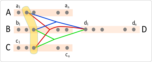
Figure 1: The reduction in the proof of Theorem 11, with $k=3$, $A_{1}=A$, $A_{2}=B$ and $A_{3}=C$. The set $\{d_{1},a_{2},b_{3},c_{3}\}$ is a simplex in $H$ because $1\in\mathbf{x}\cap\mathbf{y}$, corresponding to vertex $d_{1}$. Alice inserts the blue edge $\{d_{1},a_{2},b_{3}\}$ while encoding $\mathbf{x}$, while Bob inserts the red and green edges while encoding $\mathbf{y}$, plus the data-independent yellow edge. Similarly, $\{a_{i},b_{j},c_{k},d_{1}\}$ are simplices for all $i,j,k\in[n]$.

In the end, ${H}$ has $m=\Theta(n^{k})$ edges. Further, $T_{k}(H)$ is exactly $n^{k}$ times the size of the intersection $|\mathbf{x}\cap\mathbf{y}|$. Because of the unique intersection promise, we either have $T_{k}(H)=0$ or $T_{k}(H)=T:=n^{k}$, which proves the correctness of the reduction. Moreover, when $T_{k}(H)\neq 0$, we have $\Delta_{V}=n^{k}$.

If there existed an algorithm $\mathcal{A}$ for the simplex-dist task guaranteed to use only $o(m^{1+1/k}/T)$ bits of memory, the resulting communication protocol for $\textsc{udisj}_{n}^{n/4}$ would use $o(n^{k+1}/n^{k})=o(n)$ bits of communication, a contradiction. For the same reason, $\mathcal{A}$ could not have guaranteed a space bound of $o(m/T^{1-1/k})$ bits, nor $o(m\Delta_{V}^{1/k}/T)$ bits. ∎

A Lower Bound in Terms of the Approximation Parameter.

Finally, we show that the inverse quadratic dependence on the approximation parameter $\varepsilon$, which appears in all our algorithms (and is indeed ubiquitous in the literature on streaming algorithms) is necessary.

Theorem 12.

The task $\textsc{simplex-sep}_{k}(n,m,T,\varepsilon)$ requires $\Omega(\varepsilon^{-2}/p)$ space using $p$ passes, even when $n$ and $m$ are functions of $\varepsilon$ alone.

Proof.

We reduce from $\textsc{gap-disj}_{n,n/2,\sqrt{n}}$. We repeat the hypergraph construction in the proof of Theorem 11. As observed in that proof, the number of simplices $T_{k}(H)$ in that hypergraph $H$ is exactly $n^{k}$ times the intersection size $|\mathbf{x}\cap\mathbf{y}|$. Therefore, if $\varepsilon$ and $n$ are related by $\varepsilon=C/\sqrt{n}$, for a suitable constant $C$, then an algorithm for $\textsc{simplex-sep}_{k}(n,m,T,\varepsilon)$ solves $\textsc{gap-disj}_{n,n/2,\sqrt{n}}$. The proof is completed by invoking known communication lower bounds. ∎

7 Targeted-Sampling Algorithms Based on Hyperarboricity

In this section, we discuss in more detail the more straightforward, but trickier to analyze, targeted-sampling algorithm that was outlined in Section 2.1. It runs in space $\widetilde{O}(m^{2-1/k}/T)$, which is suboptimal, but still sublinear once $T$ is large enough.

The algorithm, formalized as Algorithm 5, is similar to Algorithm 1 in its general setup. The broad framework of its analysis is also similar to what went before. However, two key insights required in the analysis use mathematical tools from extremal hypergraph theory. Specifically, we use the idea of hyperforest packing [FKK03] to define a new quantity that we call the hyperarboricity of a hypergraph. We proceed to give a generally applicable bound on this quantity and use it to bound the space usage of our algorithm. We feel that the techniques and tools developed here may be of independent interest and value.

7.1 Definitions and Preliminaries

For $F\subseteq E$, let $V(F)$ be the set of all vertices in $V$ that belong to some hyperedge in $F$. For $S\subseteq V$, let $E(S)$ be the set of hyperedges contained completely within $S$, i.e., the set of hyperedges induced by $S$.

Recall [Bre13] that every hypergraph can be represented by a bipartite graph. The bipartite representation of $H$ is the bipartite graph $G_{H}=(V;E,R)$, where the edge $r=\{v,E\}\in R$ exists between a vertex $v$ and a hyperedge $E$ of $H$ if $v\in E$. This $G_{H}$ construction inspires the following definition.

In graph theory, a forest is an acyclic graph. Equivalently, forests are exactly the graphs in which for every subset $X$ of the edge set, the number of incident vertices is strictly greater than $|X|$. In general hypergraphs, keeping the bipartite representation in mind, we refer to this property as the strong Hall property. We shall use the corresponding definition of “hyperforests” [FKK03, Lov68, Lov70].

Definition 7.1 (Strong Hall property, hyperforest).

A hypergraph $H=(V,E)$ satisfies the strong Hall property if, for any non-empty subset $X\subseteq E$, we have that $|V(F)|>|F|$. Equivalently, for any $S\subseteq V$, we have that $|E(S)|<|S|$. A hypergraph $H$ satisfying the strong Hall property is called a hyperforest.

Note that, unlike for usual graphs (i.e., $2$-graphs), acyclicity and the strong Hall property do not coincide.

The arboricity of an ordinary graph is the minimum number of forests that its edge set can be partitioned into. The above notion of hyperforest provides a natural generalization of this quantity to hypergraphs.

Definition 7.2 (Hyperarboricity).

The hyperarboricity of a hypergraph $H$, denoted $\rho(H)$, is the minimum number of edge-disjoint hyperforests that $E(H)$ can be decomposed into.

Seeking a generalization of the classic forest-packing theorems of Tutte and Nash-Williams [CMW⁺94], Frank, Kiraly, and Kriesell [FKK03] use matroids to give the following necessary and sufficient condition for the decomposition of a hypergraph into edge-disjoint sub-hyperforests.

Lemma 7.3 (Hyperforest packing; Theorem 2.10 of [FKK03]).

The edge-set $E$ of a hypergraph $H=(V,E)$ can be decomposed into $k$ hyperforests iff $|E(X)|\leq k(|X|-1)$ for every non-empty subset $X\subseteq V$. ∎

Using this, we obtain an extremal condition that characterizes the hyperarboricity concept.

Lemma 7.4.

For every hypergraph $H$,

$$\rho(H)=\max_{H^{\prime}=(V^{\prime},E^{\prime})<H}\left\lceil\frac{|E^{\prime}|}{|V^{\prime}|-1}\right\rceil\,,$$

where “$<$” denotes the sub-hypergraph relation.

Proof.

Let $V^{\prime}\subseteq V$ and consider an arbitrary sub-hypergraph $H^{\prime}=(V^{\prime},E^{\prime})$ of the induced (by $V^{\prime}$) sub-hypergraph $H^{\prime\prime}=(V^{\prime},E^{\prime\prime})<H$. Then, $|E^{\prime}|\leq|E^{\prime\prime}|$, so by Lemma 7.3,

$$\rho(H)\geq\frac{|E^{\prime\prime}|}{|V^{\prime\prime}|-1}\geq\frac{|E^{\prime}|}{|V^{\prime}|-1}\,.$$

Since $\rho(H)$ is an integer, we arrive at our conclusion. ∎

7.2 A General Upper Bound on Hyperarboricity

In analyzing our eventual algorithm, a key portion of the combinatorial argument will need to bound a sum of the form $s_{1}$, shown in eq. 1. A classic result of Chiba and Nishizeki [CN85] bounds this sum in the special case when $H$ is an ordinary graph. For our $k$-uniform hypergraph generalization, we start with the following useful upper bound on the hyperarboricity of such a hypergraph.

Lemma 7.5.

The hyperarboricity $\rho(H)$ of an $m$-edge $k$-graph $H$ is bounded by $\rho(H)=O\left(m^{(k-1)/k}\right)$.

Proof.

Invoking Lemma 7.4, we let $H^{\prime}<H$ be a sub-hypergraph satisfying

$$\rho(H)=\left\lceil\frac{|E(H^{\prime})|}{|V(H^{\prime})|-1}\right\rceil\,.$$

Let $p=|V(H^{\prime})|$, $q=|E(H^{\prime})|$ and let $s=\binom{p}{k}$ be the number of edges on a complete $k$-uniform hypergraph with $p$ vertices. We make two algebraic observations.

• First, we observe that $p=O((s+p)^{1/k})$. This is because $s\geq Cp^{k}\geq Cp^{k}-p$ for some constant $C$, which implies that $s+p=\Omega(p^{k})$.

• Second, we observe that $k!\cdot s=O((p-1)^{k})$. This holds because $k!\cdot s=p(p-1)\cdots(p-k+1)\leq p(p-1)^{k-1}=(p-1)^{k}+(p-1)^{k-1}=O((p-1)^{k})$.

We now branch into two cases.

In the first case, $s\leq m$. Then, we have

$$\rho(H)=\left\lceil\frac{q}{p-1}\right\rceil\leq\left\lceil\frac{s}{p-1}\right\rceil \leq\left\lceil\frac{p(p-2)\cdots(p-k+1)}{k!}\right\rceil$$

$$\leq\left\lceil\frac{p^{k-1}}{k!}\right\rceil=O(p^{k-1})\,.$$

By the first observation, $p=O((s+p)^{1/k})$, giving

$$\rho(H)=O\left((s+p)^{(k-1)/k}\right)=O\left((m+n)^{(k-1)/k}\right)=O\left(m^{(k-1)/k}\right)$$

because $s\leq m,p\leq n$ and $n=O(m)$.

In the second case, $s\geq m$. By the second observation above, we get:

$$\rho(H)=\left\lceil\frac{q}{p-1}\right\rceil \leq\left\lceil\frac{m}{p-1}\right\rceil$$

$$\stackrel{{\scriptstyle m\leq s}}{{\leq}}\left\lceil\frac{ms^{\frac{1}{k-1}}}{(p-1)^{\frac{k}{k-1}}}\right\rceil^{\frac{k-1}{k}}$$

$$\leq(k!)^{-\frac{1}{k}}\left(\frac{m(p-1)^{\frac{k}{k-1}}}{(p-1)^{\frac{k}{k-1}}}\right)^{\frac{k-1}{k}}=O\left(m^{\frac{k-1}{k}}\right)\,.\qed$$

As a corollary to the above bound on hyperarboricity, we obtain the following combinatorial fact, which will be useful in our algorithmic analysis later on.

Lemma 7.6.

Let $H=(V,E)$ be a $k$-uniform hypergraph with $|E|=m$ and $|V|=n=O(m)$. Then:

$$\sum_{\{u_{1},\ldots,u_{k}\}\in E}\min\{\deg(u_{1}),\ldots,\deg(u_{k})\}\leq km\rho(H)=O(m^{2-1/k})\,.$$ (42)

Proof.

Consider a decomposition of $H$ into $\rho(H)$ hyperforests $\mathcal{F}_{i}=(V_{i},E_{i})$ for $i\in[\rho(H)]$. In each hyperforest $\mathcal{F}_{i}$, we will associate each hyperedge $e\in E_{i}$ with a representative vertex $v^{(i)}(e)\in E$ such that no two hyperedges in $E_{i}$ share a representative. We can find such a mapping from $E_{i}$ to $V_{i}$ if and only if $G_{\mathcal{F}_{i}}$ has a perfect matching that saturates $E_{i}$. Since $\mathcal{F}_{i}$ is a hyperforest, Definition 7.1 and Hall’s Matching Theorem ensure that a perfect matching saturating $E_{i}$ exists. Using Lemma 7.5 and the handshake lemma, we get:

$$\sum_{\{u_{1},\ldots,u_{k}\}\in E}\min\{\deg(u_{1}),\ldots,\deg(u_{k})\} =\sum_{1\leq i\leq\rho(H)}\sum_{\{u_{1},\ldots,u_{k}\}\in E_{i}}\min\{\deg(u_{1}),\ldots,\deg(u_{k})\}$$

$$\leq\sum_{1\leq i\leq\rho(H)}\sum_{e\in E_{i}}\deg(v^{(i)}(e))$$

$$\leq\sum_{1\leq i\leq\rho(H)}\sum_{v\in V}\deg(v)=km\rho(H)=O\left(m^{2-1/k}\right)\,.\qed$$

Remark.

This bound is tight. Equality holds for complete $k$-graphs.

7.3 The Algorithm Based on Global Degree Ordering

We are ready to give the details of our algorithm. Having seen an outline of the technique in Section 2.1 and a detailed description of a more elaborate algorithm in a similar vein in Section 4, we are prepared to dive right in to the formal description. This is given in Algorithm 5. The main new piece of notation here is “$\prec$” which denotes a total ordering on $V$ according to the degrees of the vertices, settling ties by comparing IDs.

1:procedure $k$-Simplex-Count-Easy($\sigma$)

2:     pass 1: $\triangleright$ $O(1)$ space      

3:         pick an edge $e=\{u_{1},u_{2},\ldots,u_{k}\}\in E$ using reservoir sampling      

4:     pass 2: $\triangleright$ $O(1)$ space      

5:         calculate the degrees $\deg(u_{1}),\deg(u_{2}),\ldots,\deg(u_{k})$      

6:     pass 3: $\triangleright$ $\widetilde{O}(R)$ space      

7:         $R\leftarrow\left\lceil\min\{\deg(u_{1}),\deg(u_{2}),\ldots,\deg(u_{k})\}\cdot m^{-1/2}\right\rceil$

8:         re-arrange (if needed) $u_{1},u_{2},\ldots,u_{k}$ so that $u_{1}\prec u_{2}\prec\cdots\prec u_{k}$

9:         for $j=1$ to $R$, in parallel, do

10:              $Z_{j}\leftarrow 0$

11:              construct a virtual stream $\sigma_{j}$ of the vertices in $\operatorname{N}(u_{1})\smallsetminus\{u_{2},\ldots,u_{k}\}$

12:              sample vertex $x_{j}$ from $\operatorname{N}(u_{1})\smallsetminus\{u_{2},\ldots,u_{k}\}$ u.a.r., using $\ell_{0}$-sampling on $\sigma_{j}$          

13:         in parallel, approximate $|\operatorname{N}(u_{1})|$ using $F_{0}$-estimation      

14:     pass 4: $\triangleright$ $O(R)$ space      

15:         compute the degrees $\deg(x_{1}),\deg(x_{2}),\ldots,\deg(x_{R})$

16:         for $j=1$ to $R$, in parallel, do

17:              if $u_{k}\prec x_{j}$ and $\{u_{1},u_{2},\ldots,u_{k},x_{j}\}$ form a $k$-simplex then

18:                  $Z_{j}\leftarrow|\operatorname{N}(u_{1})|-k+1$ $\triangleright$ $u_{1}$ has the smallest degree                             

19:     return $Y\leftarrow(m/R)\sum_{j=1}^{R}Z_{j}$ $\triangleright$ Average out the trials and scale

Algorithm 5 Counting simplices in $k$-uniform hypergraph streams the easy (and suboptimal) way

One subtlety in this algorithm, which does not show up in the corresponding (and much simpler) algorithm for graphs [BC17], is the uniform sampling of the vertex in the neighborhood of $u_{1}$ (lines 11–12). In graphs, reservoir sampling suffices because sampling a neighbor of $u_{1}$ is equivalent to sampling uniformly an edge that is incident on $u$. The same is not true for hypergraphs, because sampling a hyperedge uniformly from $\operatorname{N}(u_{1})$ gives a probabilistic advantage to vertices that share many hyperedges with $u_{1}$. Thus, we need to use $\ell_{0}$-sampling techniques in a substream consisting of neighbors of $u_{1}$.

A second caveat that appears is in the calculation of the size of the neighborhood of $u_{1}$. Treating every edge containing $u_{1}$ as an element in a virtual stream $\sigma_{u_{1}}$, we can calculate $|\operatorname{N}(u_{1})|$ by counting the distinct elements in $\sigma_{u_{1}}$. This can be done either precisely, in $O(n)$ space, or approximately in $\widetilde{O}(1)$ space, using an $F_{0}$-estimation algorithm.

7.4 Analysis of the Algorithm

Our analysis proceeds almost exactly like Section 4.2 The only differences are the presence of $\ell_{0}$-sampling, $F_{0}$ estimation, and the use of the upper bounds in Section 7.2.

Remark.

In the analysis below, we will assume that the algorithms for $\ell_{0}$ sampling and $F_{0}$ estimation produce the desired outputs correctly. Any precision errors are assumed to be absorbed into the quality of the estimator $Y$. Our analysis does not examine the implications of this assumption in a more pedantic way so that we can focus on the salient points of the algorithm.

Unbiased Estimator.

First we prove that our estimator $Y$ is unbiased. Define the label of a simplex $\Xi$ to be $(e,x)$ where $x$ is the $\prec$-maximal vertex in $\Xi$ and $e=\Xi\smallsetminus\{x\}$. For each $e\in E$, let $\tau_{e}$ denote the number of simplices with a label of the form $(e,\cdot)$. Let $\mathcal{E}_{e}$ denote the event that the hyperedge sampled in pass 1 is $e$. When $\mathcal{E}_{e}$ occurs, the $\ell_{0}$-sampling in 12 of Algorithm 5 causes us to pick one of the $|\operatorname{N}(u_{1})|-k+1$ vertices in $\operatorname{N}(u_{1})\smallsetminus e$ uniformly at random and exactly $\tau_{e}$ of these vertices complete a valid simplex label with hyperedge $e$ (per the logic in 17). Therefore,

$$\mathbb{E}[Z_{k}\mid{\mathcal{E}}_{e}]=\tau_{e}\frac{1}{|\operatorname{N}(u_{1})|-k+1}(|\operatorname{N}(u_{1})|-k+1)=\tau_{e}\,,$$ (43)

and so, by the law of total expectation,

$$\mathbb{E}[Y]=\frac{m}{R}\sum_{j=1}^{R}\sum_{e\in E}\frac{1}{m}\mathbb{E}[Z_{j}\mid{\mathcal{E}}_{e}]=\frac{1}{R}\sum_{j=1}^{R}\sum_{e\in E}\tau_{e}=T_{k}(H)\,.$$ (44)

Bounded variance.

Now we attempt to bound the variance. Proceeding along similar lines as above,

$$\mathbb{E}[Z_{j}^{2}\mid\mathcal{E}_{e}] =(|\operatorname{N}(u_{1})|-k+1)\cdot\tau_{e}$$

$$\leq|\operatorname{N}(u_{1})|\cdot\tau_{e}\,,\quad\text{and}$$

$$\mathbb{E}[Z_{j_{1}}Z_{j_{2}}\mid\mathcal{E}_{e}] =\tau_{e}^{2}\,,$$

because $Z_{j_{1}}$ and $Z_{j_{2}}$ are independent events even when conditioned on $\mathcal{E}_{e}$. So we have

$$\mathbb{E}[Y^{2}\mid\mathcal{E}_{e}] =\mathbb{E}\left[\left(\frac{m}{R}\sum_{k=1}^{R}Z_{k}\right)^{2}\,\middle|\,\mathcal{E}_{e}\right]$$

$$=\frac{m^{2}}{R^{2}}\sum_{j=1}^{R}\mathbb{E}[Z_{j}^{2}\mid\mathcal{E}_{e}]+\frac{m^{2}}{R^{2}}\sum_{j_{1}\neq j_{2}}\mathbb{E}[Z_{j_{1}}Z_{j_{2}}\mid\mathcal{E}_{e}]$$

$$\leq\frac{m^{2}|\operatorname{N}(u_{1})|\cdot\tau_{e}}{R}+\frac{m^{2}R(R-1)\tau_{e}^{2}}{R^{2}}$$

$$\leq(k-1)m^{5/2}\tau_{e}+m^{2}\tau_{e}^{2}$$

where the final step uses $|\operatorname{N}(u_{1})|/R\leq(k-1)\deg(u_{1})/R\leq(k-1)\sqrt{m}$, by the definition of $R$. Next, using the law of total expectation, we obtain

$$\operatorname{Var}[Y]\leq\mathbb{E}[Y^{2}] =\sum_{e\in E}\frac{1}{m}\mathbb{E}[Y^{2}\mid\mathcal{E}_{e}]$$

$$\leq(k-1)m^{3/2}\sum_{e\in E}\tau_{e}+m\sum_{e\in E}\tau_{e}^{2}$$

$$\leq(k-1)m^{3/2}T_{k}(H)+m\sum_{e\in E}\tau_{e}^{2}\,.$$ (45)

At this point we need a bound on $\sum\tau_{e}^{2}$. To that end, we will use the following lemma.

Lemma 7.7.

Let $S_{u_{1}}:=\{w\in\operatorname{N}(u_{1})\mid u_{1}\prec w\}$ be the set of neighbors of $u_{1}$ that are after it in the total ordering of vertices based on degree. Then $|S_{u_{1}}|=O\left(\sqrt{m}\right)$.

Proof.

We know that for each $w\in S_{u_{1}}$,

$$\deg(w)\geq\deg(u_{1})\geq\frac{|\operatorname{N}(u_{1})|}{k-1}\geq\frac{|S_{u_{1}}|}{k-1}\,,$$

Thus, by the handshake lemma, we have

$$km\geq\sum_{w\in S_{u_{1}}}\deg(w)\geq|S_{u_{1}}|\left(\frac{|S_{u_{1}}|}{k-1}\right)\,,$$

implying $|S_{u_{1}}|=O(\sqrt{m})$. ∎

Using Lemma 7.7, we obtain that

$$\sum_{e\in E}\tau_{e}^{2}=O\left(T_{k}(H)\sqrt{m}\right)$$ (46)

because, for each edge $e$, we have that $\tau_{e}\leq|S_{u_{1}}|=O(\sqrt{m})$, where we use $S_{u_{1}}$ as in the proof of Lemma 7.7. Finally, plugging the bound (46) into eq. 45, we conclude that

$$\operatorname{Var}[Y]=O\left(m^{3/2}T_{k}(H)\right)\,.$$ (47)

Space Complexity.

Using the median-of-means improvement, given as Lemma 3.7, we can see that our algorithm uses space $O(m^{3/2}B/T)$ to output an $(\varepsilon,1/3)$-approximation to $T_{k}(H)$, where

$$B=O(\text{space}(F_{0}\text{-estimation})+R\cdot\text{space}(\ell_{0}\text{-sampling}))$$ (48)

is the space used by one instance of Algorithm 5. For simplicity, assume that the $F_{0}$-estimation and $\ell_{0}$-sampling procedures function perfectly (this does not affect the ultimate asymptotic results). Using known results and hiding the dependence on accuracy parameters, we have space$(F_{0}$-estimation$)=O(\log n)$ and space$(\ell_{0}$-sampling$)=O(\log^{2}n)$. It remains to bound $\mathbb{E}[R]$. We have that

$$\mathbb{E}[R] =\frac{1}{m}\sum_{\{u_{1},\ldots,u_{k}\}\in E}\left\lceil\frac{\min\Big{\{}\deg(u_{1}),\ldots,\deg(u_{k})\Big{\}}}{\sqrt{m}}\right\rceil$$

$$=O\left(m^{-3/2}\sum_{\{u_{1},\ldots,u_{k}\}\in E}\min\Big{\{}\deg(u_{1}),\ldots,\deg(u_{k})\Big{\}}\right)\,.$$

This is where our work using hyperarboricity comes in. Using Lemma 7.6, we get that

$$\mathbb{E}[R]=O\left(m^{2-\frac{1}{k}-\frac{3}{2}}\right)=O\left(m^{\frac{1}{2}-\frac{1}{k}}\right)\,.$$

Plugging this into Equation 48, we get

$$\mathbb{E}[B]=O\left(\log n+m^{\frac{1}{2}-\frac{1}{k}}\log^{2}n\right)=\widetilde{O}\left(m^{\frac{1}{2}-\frac{1}{k}}\right)\,.$$

We have thus arrived at the following theorem.

Theorem 13.

There is a $4$-pass streaming algorithm that $(\varepsilon,\delta)$-approximates the number of simplices in a $k$-uniform hypergraph $H$ using $\widetilde{O}\big{(}m^{2-1/k}/T\big{)}$ space, under the promise that $T_{k}(H)\geq T$. ∎

8 Concluding Remarks

We initiated a systematic study of the problem of counting simplices in a hypergraph given as an edge stream, a natural generalization of the much-studied triangle counting problem. We obtained several sublinear-space algorithms for the problem: which of them is best depends on some combinatorial parameters of the problem instance. Overall, we learned that established methods for triangle and substructure counting in graph streams are not by themselves enough and considerable effort is required to deal with the more intricate structures occurring in hypergraphs.

In some parameter regimes (what we called the “abundant” case), we obtained provably space-optimal algorithms. However, in the “meager” case, seeking algorithms with space complexity of the form $m/T^{\lambda}$, we established an upper bound with $\lambda=2/(k+1)$ and a lower bound with $\lambda=1-1/k$. Closing this gap seems to us to be the most compelling follow-up research question.

The simplex counting problem has the potential to impact research on pattern detection and enumeration. As triangle counting has done in the past two decades, simplex counting may offer new insights on how sampling techniques can exploit the structure of graphs and hypergraphs to extract meaningful information.

References

- [Abl96] Farid Ablayev. Lower bounds for one-way probabilistic communication complexity and their application to space complexity. Theor. Comput. Sci., 175(2):139–159, 1996.
- [AKK19] Sepehr Assadi, Michael Kapralov, and Sanjeev Khanna. A simple sublinear-time algorithm for counting arbitrary subgraphs via edge sampling. In Proc. 10th Conference on Innovations in Theoretical Computer Science, volume 124 of LIPIcs, pages 6:1–6:20. Schloss Dagstuhl - Leibniz-Zentrum für Informatik, 2019.
- [AYZ97] Noga Alon, Raphael Yuster, and Uri Zwick. Finding and counting given length cycles. Algorithmica, 17(3):209–223, 1997. Preliminary version in Proc. 2nd Annual European Symposium on Algorithms, pages 354–364, 1994.
- [BBCG08] Luca Becchetti, Paolo Boldi, Carlos Castillo, and Aristides Gionis. Efficient semi-streaming algorithms for local triangle counting in massive graphs. In Proc. 14th Annual SIGKDD International Conference on Knowledge Discovery and Data Mining, pages 16–24, 2008.
- [BC17] Suman K. Bera and Amit Chakrabarti. Towards tighter space bounds for counting triangles and other substructures in graph streams. In Proc. 34th International Symposium on Theoretical Aspects of Computer Science, pages 11:1–11:14, 2017.
- [BFKP16] Laurent Bulteau, Vincent Froese, Konstantin Kutzkov, and Rasmus Pagh. Triangle counting in dynamic graph streams. Algorithmica, 76(1):259–278, 2016.
- [BFL+06] Luciana S. Buriol, Gereon Frahling, Stefano Leonardi, Alberto Marchetti-Spaccamela, and Christian Sohler. Counting triangles in data streams. In Proc. 25th ACM Symposium on Principles of Database Systems, pages 253–262, 2006.
- [BKS02] Ziv Bar-Yossef, Ravi Kumar, and D. Sivakumar. Reductions in streaming algorithms, with an application to counting triangles in graphs. In Proc. 13th Annual ACM-SIAM Symposium on Discrete Algorithms, pages 623–632, 2002.
- [BOV13] Vladimir Braverman, Rafail Ostrovsky, and Dan Vilenchik. How hard is counting triangles in the streaming model? In Proc. 40th International Colloquium on Automata, Languages and Programming, pages 244–254. Springer, 2013.
- [Bre13] Alain Bretto. Hypergraph Theory: An Introduction. Mathematical Engineering. Springer International Publishing, 2013.
- [CF10] Nicholas A Christakis and James H Fowler. Social network sensors for early detection of contagious outbreaks. PLoS ONE, 5(9):e12948, 2010.
- [CJ14] Graham Cormode and Hossein Jowhari. A second look at counting triangles in graph streams. Theor. Comput. Sci., 552:44–51, 2014.
- [CJ17] Graham Cormode and Hossein Jowhari. A second look at counting triangles in graph streams (corrected). Theor. Comput. Sci., 683:22–30, 2017.
- [CMW+94] Boliong Chen, Makoto Matsumoto, Jianfang Wang, Jianxun Zhang, and Zhongfu Zhang. A short proof of Nash-Williams’ theorem for the arboricity of a graph. Graphs and Combinatorics, 10(1):27–28, 1994.
- [CN85] Norishige Chiba and Takao Nishizeki. Arboricity and subgraph listing algorithms. SIAM J. Comput., 14(1):210–223, 1985.
- [CR12] Amit Chakrabarti and Oded Regev. An optimal lower bound on the communication complexity of gap-hamming-distance. SIAM J. Comput., 41(5):1299–1317, 2012. Preliminary version in Proc. 43rd Annual ACM Symposium on the Theory of Computing, pages 51–60, 2011.
- [DKPW20] Lech Duraj, Krzysztof Kleiner, Adam Polak, and Virginia Vassilevska Williams. Equivalences between triangle and range query problems. In Shuchi Chawla, editor, Proc. 31st Annual ACM-SIAM Symposium on Discrete Algorithms, pages 30–47. SIAM, 2020.
- [ELRS15] Talya Eden, Amit Levi, Dana Ron, and C. Seshadhri. Approximately counting triangles in sublinear time. In IEEE 56th Annual Symposium on Foundations of Computer Science, FOCS 2015, Berkeley, CA, USA, 17-20 October, 2015, pages 614–633, 2015.
- [ERS20] Talya Eden, Dana Ron, and C. Seshadhri. On approximating the number of k-cliques in sublinear time. SIAM J. Comput., 49(4):747–771, 2020.
- [Fis89] David C. Fisher. Lower bounds on the number of triangles in a graph. J. Graph Th., 13(4):505–512, 1989.
- [FKK03] András Frank, Tamás Király, and Matthias Kriesell. On decomposing a hypergraph into k connected sub-hypergraphs. Discrete Applied Mathematics, 131(2):373–383, 2003.
- [GP18] Allan Grønlund and Seth Pettie. Threesomes, degenerates, and love triangles. J. ACM, 65(4):22:1–22:25, 2018.
- [GZY+19] Chuangyi Gui, Long Zheng, Pengcheng Yao, Xiaofei Liao, and Hai Jin. Fast triangle counting on GPU. In 2019 IEEE High Performance Extreme Computing Conference, HPEC 2019, Waltham, MA, USA, September 24-26, 2019, pages 1–7. IEEE, 2019.
- [JG05] Hossein Jowhari and Mohammad Ghodsi. New streaming algorithms for counting triangles in graphs. In Lusheng Wang, editor, Proc. 11th Annual International Conference on Computing and Combinatorics (COCOON), pages 710–716, 2005.
- [JK21] Rajesh Jayaram and John Kallaugher. An optimal algorithm for triangle counting in the stream. In Proc. 24th International Workshop on Approximation Algorithms for Combinatorial Optimization Problems, volume 207 of LIPIcs, pages 11:1–11:11, 2021.
- [JSP15] Madhav Jha, C. Seshadhri, and Ali Pinar. A space-efficient streaming algorithm for estimating transitivity and triangle counts using the birthday paradox. ACM Trans. Knowl. Discov. Data, 9(3):15:1–15:21, 2015.
- [KKP18] John Kallaugher, Michael Kapralov, and Eric Price. The sketching complexity of graph and hypergraph counting. In Proc. 59th Annual IEEE Symposium on Foundations of Computer Science, pages 556–567. IEEE Computer Society, 2018.
- [KMPT12] Mihail N. Kolountzakis, Gary L. Miller, Richard Peng, and Charalampos E. Tsourakakis. Efficient triangle counting in large graphs via degree-based vertex partitioning. Internet Mathematics, 8(1-2):161–185, 2012.
- [KMPV19] John Kallaugher, Andrew McGregor, Eric Price, and Sofya Vorotnikova. The complexity of counting cycles in the adjacency list streaming model. In Dan Suciu, Sebastian Skritek, and Christoph Koch, editors, Proc. 38th ACM Symposium on Principles of Database Systems, pages 119–133. ACM, 2019.
- [KMSS12] Daniel M. Kane, Kurt Mehlhorn, Thomas Sauerwald, and He Sun. Counting arbitrary subgraphs in data streams. In Artur Czumaj, Kurt Mehlhorn, Andrew M. Pitts, and Roger Wattenhofer, editors, Proc. 39th International Colloquium on Automata, Languages and Programming, volume 7392 of Lecture Notes in Computer Science, pages 598–609. Springer, 2012.
- [KP17] John Kallaugher and Eric Price. A hybrid sampling scheme for triangle counting. In Proceedings of the Twenty-Eighth Annual ACM-SIAM Symposium on Discrete Algorithms, pages 1778–1797. SIAM, 2017.
- [KV04] Jeong Han Kim and Van H. Vu. Divide and conquer martingales and the number of triangles in a random graph. Rand. Struct. Alg., 24(2):166–174, 2004.
- [LHK10] Jure Leskovec, Daniel Huttenlocher, and Jon Kleinberg. Predicting positive and negative links in online social networks. In Proc. 19th International Conference on World Wide Web (WWW), pages 641–650, 2010.
- [Lov68] László Lovász. On chromatic number of finite set-systems. Acta Mathematica Academiae Scientiarum Hungarica, 19(1-2):59–67, 1968.
- [Lov70] László Lovász. A generalization of Kónig’s theorem. Acta Mathematica Academiae Scientiarum Hungarica, 21(3-4):443–446, 1970.
- [Man07] Willem Mantel. Problem 28 (solution by H. Gouweniak, W. Mantel, J. Texeira de Mattes, F. Schuh, and WA Whythoff). Wiskundige Opgaven, 10:60–61, 1907.
- [MMPS11] Madhusudan Manjunath, Kurt Mehlhorn, Konstantinos Panagiotou, and He Sun. Approximate counting of cycles in streams. In Camil Demetrescu and Magnús M. Halldórsson, editors, Proc. 19th Annual European Symposium on Algorithms, volume 6942 of Lecture Notes in Computer Science, pages 677–688. Springer, 2011.
- [MVV16] Andrew McGregor, Sofya Vorotnikova, and Hoa T. Vu. Better algorithms for counting triangles in data streams. In Proc. 35th ACM Symposium on Principles of Database Systems, pages 401–411, 2016.
- [New03] Mark EJ Newman. The structure and function of complex networks. SIAM review, 45(2):167–256, 2003.
- [NPRR18] Hung Q. Ngo, Ely Porat, Christopher Ré, and Atri Rudra. Worst-case optimal join algorithms. J. ACM, 65(3):16:1–16:40, 2018.
- [PT12] Rasmus Pagh and Charalampos E. Tsourakakis. Colorful triangle counting and a MapReduce implementation. Information Processing Letters, 112(7):277–281, 2012.
- [PTTW13] A. Pavan, Kanat Tangwongsan, Srikanta Tirthapura, and Kun-Lung Wu. Counting and sampling triangles from a graph stream. Proc. VLDB Endowment, 6(14):1870–1881, 2013.
- [Raz92] Alexander Razborov. On the distributional complexity of disjointness. Theor. Comput. Sci., 106(2):385–390, 1992. Preliminary version in Proc. 17th International Colloquium on Automata, Languages and Programming, pages 249–253, 1990.
- [Raz08] Alexander A. Razborov. On the minimal density of triangles in graphs. Comb. Probab. Comput., 17(4):603–618, 2008.
- [RH03] Jacques Rougemont and Pascal Hingamp. Dna microarray data and contextual analysis of correlation graphs. BMC bioinformatics, 4(1):1–11, 2003.
- [SPK14] C. Seshadhri, Ali Pinar, and Tamara G. Kolda. Wedge sampling for computing clustering coefficients and triangle counts on large graphs. Stat. Anal. Data Min., 7(4):294–307, 2014.
- [SV11] Siddharth Suri and Sergei Vassilvitskii. Counting triangles and the curse of the last reducer. In Proc. 20th International Conference on World Wide Web (WWW), pages 607–614. ACM, 2011.
- [TKM11] Charalampos E. Tsourakakis, Mihail N. Kolountzakis, and Gary L. Miller. Triangle sparsifiers. J. Graph Algorithms Appl., 15(6):703–726, 2011.
- [Vor20] Sofya Vorotnikova. Improved 3-pass algorithm for counting 4-cycles in arbitrary order streaming. CoRR, abs/2007.13466, 2020.
- [WCW+18] Zhiang Wu, Jie Cao, Yaqiong Wang, Youquan Wang, Lu Zhang, and Junjie Wu. hPSD: a hybrid pu-learning-based spammer detection model for product reviews. IEEE transactions on cybernetics, 50(4):1595–1606, 2018.
- [Wil21] Virginia Vassilevska Williams. 3sum and related problems in fine-grained complexity (invited talk). In Proc. 37th ACM Symposium on Computational Geometry, volume 189 of LIPIcs, pages 2:1–2:2. Schloss Dagstuhl - Leibniz-Zentrum für Informatik, 2021.