MPViT : Multi-Path Vision Transformer for Dense Prediction

Abstract

Dense computer vision tasks such as object detection and segmentation require effective multi-scale feature representation for detecting or classifying objects or regions with varying sizes. While Convolutional Neural Networks (CNNs) have been the dominant architectures for such tasks, recently introduced Vision Transformers (ViTs) aim to replace them as a backbone. Similar to CNNs, ViTs build a simple multi-stage structure (i.e., fine-to-coarse) for multi-scale representation with single-scale patches. In this work, with a different perspective from existing Transformers, we explore multi-scale patch embedding and multi-path structure, constructing the Multi-Path Vision Transformer (MPViT). MPViT embeds features of the same size (i.e., sequence length) with patches of different scales simultaneously by using overlapping convolutional patch embedding. Tokens of different scales are then independently fed into the Transformer encoders via multiple paths and the resulting features are aggregated, enabling both fine and coarse feature representations at the same feature level. Thanks to the diverse, multi-scale feature representations, our MPViTs scaling from tiny (5M) to base (73M) consistently achieve superior performance over state-of-the-art Vision Transformers on ImageNet classification, object detection, instance segmentation, and semantic segmentation. These extensive results demonstrate that MPViT can serve as a versatile backbone network for various vision tasks. Code will be made publicly available at https://git.io/MPViT.

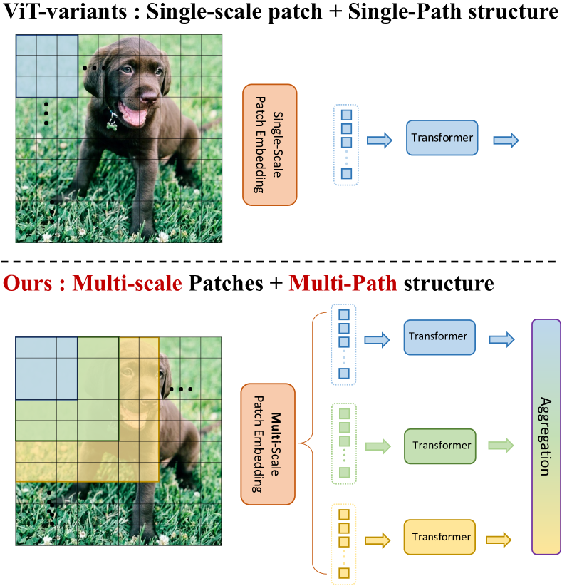
Figure 1: Top: The state-of-the-art ViT-variants [60, 37, 67] use single-scale patches and single-path Transformer encoders. Bottom: MPViT uses multi-scale patch embedding, each embedded patch following a path to an independent Transformer encoder, allowing simulatneous representations of fine and coarse features.

1 Introduction

Since its introduction, the Transformer [53] has had a huge impact on natural language processing (NLP) [14, 43, 4]. Likewise, the advent of Vision Transformer (ViT) [16] has moved the computer vision community forward. As a result, there has been a recent explosion in Transformer-based vision works, spanning tasks such as static image classification [58, 57, 37, 67, 65, 17, 50, 51], object detection [74, 5, 12], and semantic segmentation [54, 63] to temporal tasks such as video classification [3, 1, 18] and object tracking [41, 56, 7].

It is crucial for dense prediction tasks such as object detection and segmentation to represent features at multiple scales for discriminating between objects or regions of varying sizes. Modern CNN backbones which show better performance for dense prediction leverage multiple scales at the convolutional kernel level [47, 46, 33, 32, 19], or feature level [55, 42, 34]. Inception Network [46] or VoVNet [32] exploits multi-grained convolution kernels at the same feature level, yielding diverse receptive fields and in turn boosting detection performance. HRNet [55] represents multi-scale features by simultaneously aggregating fine and coarse features throughout the convolutional layers.

Although CNN models are widely utilized as feature extractors for dense predictions, the current state-of-the-art (SOTA) Vision Transformers [58, 57, 71, 37, 60, 67, 65, 17] have surpassed the performance of CNNs. While the ViT-variants [58, 60, 71, 37, 67, 17] focus on how to address the quadratic complexity of self-attention when applied to dense prediction with a high-resolution, they pay less attention to building effective multi-scale representations. For example, following conventional CNNs [44, 23], recent Vision Transformer backbones  [58, 71, 37, 67] build a simple multi-stage structure (e.g., fine-to-coarse structure) with single-scale patches (i.e., tokens). CoaT [65] simultaneously represents fine and coarse features by using a co-scale mechanism allowing cross-layer attention in parallel, boosting detection performance. However, the co-scale mechanism requires heavy computation and memory overhead as it adds extra cross-layer attention to the base models (e.g., CoaT-Lite). Thus, there is still room for improvement in multi-scale feature representation for ViT architectures.

In this work, we focus on how to effectively represent multi-scale features with Vision Transformers for dense prediction tasks. Inspired by CNN models exploiting the multi-grained convolution kernels for multiple receptive fields [46, 32, 19], we propose a multi-scale patch embedding and multi-path structure scheme for Transformers, called Multi-Path Vision Transformer (MPViT). As shown in Fig. 1, the multi-scale patch embedding tokenizes the visual patches of different sizes at the same time by overlapping convolution operations, yielding features having the same sequence length (i.e., feature resolution) after properly adjusting the padding/stride of the convolution. Then, tokens from different scales are independently fed into Transformer encoders in parallel. Each Transformer encoder with different-sized patches performs global self-attention. Resulting features are then aggregated, enabling both fine and coarse feature representations at the same feature level. In the feature aggregation step, we introduce a global-to-local feature interaction (GLI) process which concatenates convolutional local features to the transformer’s global features, taking advantage of both the local connectivity of convolutions and the global context of the transformer.

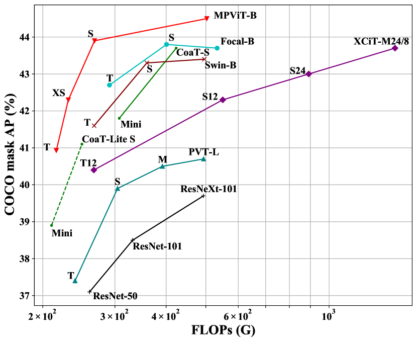
Figure 2: FLOPs vs. COCO mask AP on Mask R-CNN. MPViTs outperform state-of-the-art Vision Transformers while having fewer parameters and FLOPs. B, S, XS, and T at the end of the model names denote base, small, extra-small and tiny respectively. Complete results are in Table 3.

42.5(147,66.5)

Model mAP Param. GFLOPs CoaT-Lite S [65] 41.1   40M   249 CoaT-S [65] 43.7   42M   423 Swin-B [37] 43.4 107M   496 Focal-B [67] 43.7 110M   533 XCiT-M24/8 [17] 43.7   99M 1448 MPViT-S (ours) 43.9   43M   268

Following the standard training recipe as in DeiT [50], we train MPViTs on ImageNet-1K [13], which consistently achieve superior performance compared to recent SOTA Vision Transformers [37, 67, 17, 65, 60]. Furthermore, We validate MPViT as a backbone on object detection and instance segmentation on the COCO dataset and semantic segmentation on the ADE20K dataset, achieving state-the-art performance. In particular, MPViT-Small (22M & 4GFLOPs) surpasses the recent, and much larger, SOTA Focal-Base [67] (89M & 16GFLOPs) as shown in Fig. 2.

To summarize, our main contributions are as follows:

• We propose a multi-scale embedding with a multi-path structure for simultaneously representing fine and coarse features for dense prediction tasks.

• We introduce global-to-local feature interaction (GLI) to take advantage of both the local connectivity of convolutions and the global context of the transformer.

• We provide ablation studies and qualitative analysis, analyzing the effects of different path dimensions and patch scales, discovering efficient and effective configurations.

• We verify the effectiveness of MPViT as a backbone of dense prediction tasks, achieving state-of-the-art performance on ImageNet classification, COCO detection and ADE20K segmentation.

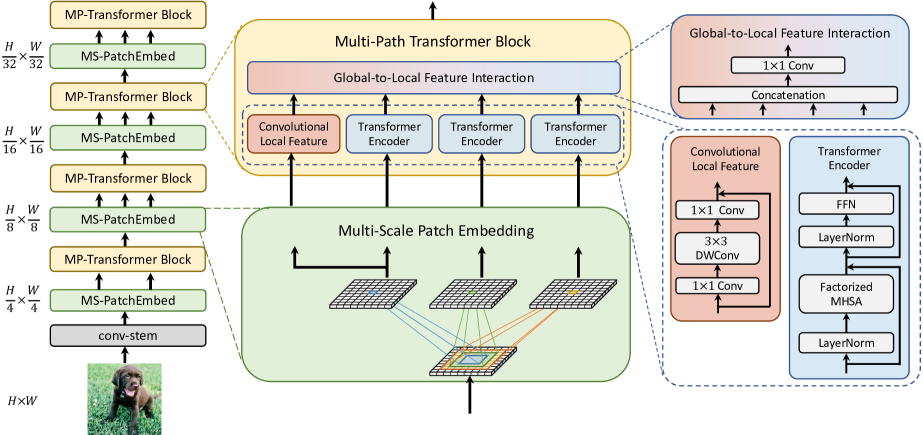
Figure 3: Overview of Multi-Path Vision Transformer (MPViT). MPViT consists of multi-scale patch embedding (MS-PatchEmbed) and multi-path transformer (MP-Transformer) blocks, which output features from each of the four stages for dense prediction tasks. Transformer encoders utilize factorized multi-head self-attention (MHSA) [65]. We omit the convoultional position encodings for simplicity.

2 Related works

Vision Transformers for dense predictions

Current SOTA Vision Transformers [58, 71, 37, 67, 65, 17] have focused on reducing the quadratic complexity of self-attention when applied to dense prediction with a high-resolution. [37, 71, 67] constrain the attention range with fine-grained patches in local regions and combine this with sliding windows or sparse global attention. [58, 60] exploit a coarse-grained global self-attention by reducing sequence length with spatial reduction (i.e., pooling). [65, 17] realizes linear complexity by operating the self-attention across feature channels rather than tokens. While [58, 71, 37, 67] has a simple pyramid structure (fine-to-coarse), XCiT [17] has a single-stage structure as ViT [16]. When applied to dense prediction tasks, XCiT adds down-/up-sampling layers to extract multi-scale features after pre-training on ImageNet. Xu et al. [65] introduce both CoaT-Lite with a simple pyramid structure and CoaT with cross-layer attention on top of CoaT-Lite. The cross-layer attention allows CoaT to outperform CoaT-Lite, but requires heavy memory and computation overhead, which limits scaling of the model.

Comparison to Concurrent work. CrossViT [6] also utilizes different patch sizes (e.g., small and large) and dual-paths in a single-stage structure as ViT [16] and XCiT [17]. However, CrossViT’s interactions between branches only occur through [CLS] tokens, while MPViT allows all patches of different scales to interact. Also, unlike CrossViT  (classification only), MPViT explores larger path dimensions (e.g., over two) more generally and adopts multi-stage structure for dense predictions.

3 Multi-Path Vision Transformer

3.1 Architecture

Fig. 3 shows the Multi-Path Vision Transformer (MPViT) architecture. Since our aim is to explore a powerful backbone network for dense predictions, we construct a multi-stage architecture [58, 37, 67] instead of a single-stage (i.e., monolithic) one such as ViT [16] and XCiT [17]. Specifically, we build a four-stage feature hierarchy for generating feature maps of different scales. As a multi-stage architecture has features with higher resolutions, it requires inherently more computation. Thus, we use Transformer encoders including factorized self-attention as done in CoaT [65] for the entire model due to its linear complexity. In LeViT [20], a convolutional stem block shows better low-level representation (i.e., without losing salient information) than non-overlapping patch embedding. Inspired by LeViT, given an input image with the size of $H\times W\times 3$, we also adopt a stem block which consists of two $3\times 3$ convolutional layers with channels of $C_{2}/2,C_{2}$ and stride of 2 which generates a feature with the size of $H/4\times W/4\times C_{2}$ where $C_{2}$ is the channel size at stage 2. Each convolution is followed by Batch Normalization [29] and a Hardswish [25] activation function. From stage 2 to stage 5, we stack the proposed multi-scale patch embedding (MS-PatchEmbed) and multi-path Transformer (MP-Transformer) blocks in each stage. Many works [16, 20, 58, 8] have proved that replacing the [CLS] token with a global average pooling (GAP) of the final feature map does not affect performance, so we also remove the [CLS] token and use GAP for simplicity.

3.2 Multi-Scale Patch Embedding

We devise a multi-scale patch embedding (MS-PatchEmbed) layer that exploits both fine- and coarse-grained visual tokens at the same feature level. To this end, we use convolution operations with overlapping patches, similar to CNNs [44, 23] and CvT [60]. Specifically, given a 2D-reshaped output feature map (i.e., token map) from a previous stage $\mathrm{X}_{i}\in\mathbb{R}^{H_{i-1}\times W_{i-1}\times C_{i-1}}$ as the input to stage $i$, we learn a function $F_{k\times k}(\cdot)$ that maps $\mathrm{X}_{i}$ into new tokens $F_{k\times k}(\mathrm{X}_{i})$ with a channel size $C_{i}$, where $F(\cdot)$ is 2D convolution operation of kernel size (i.e., patch size) $k\times k$, stride $s$ and padding $p$. The output 2D token map $F_{k\times k}(\mathrm{X}_{i})\in\mathbb{R}^{H_{i}\times W_{i}\times C_{i}}$ has height and width as below:

$$H_{i}=\lfloor\frac{H_{i-1}-k+2p}{s}+1\rfloor,W_{i}=\lfloor\frac{W_{i-1}-k+2p}{s}+1\rfloor.$$ (1)

The convolutional patch embedding layer enables us to adjust the sequence length of tokens by changing stride and padding. i.e., it is possible to output the features of the same size (i.e., resolution) with different patch sizes. Thus, we form several convolutional patch embedding layers with different kernel sizes in parallel. For example, as shown in Fig. 1, we can generate various-sized visual tokens of the same sequence length with $3\times 3,5\times 5,7\times 7$ patch sizes.

Since stacking consecutive convolution operations with the same channel and filter sizes enlarges receptive field (e.g., two $3\times 3$ are equivalent to $5\times 5$) and requires fewer parameters (e.g., $2\times 3^{2}<5^{2}$), we choose consecutive $3\times 3$ convolution layers in practice. For the triple-path structure, we use three consecutive $3\times 3$ convolutions with the same channel size $C^{\prime}$, padding of 1 and stride of $s$ where $s$ is 2 when reducing spatial resolution otherwise 1. Thus, given a feature $\mathrm{X}_{i}\in\mathbb{R}^{H_{i}\times W_{i}\times C_{i}}$ at stage $i$, we can get $F_{3\times 3}(\mathrm{X}_{i}),F_{5\times 5}(\mathrm{X}_{i}),F_{7\times 7}(\mathrm{X}_{i})$ features with the same size of $\frac{H_{i}}{s}\times\frac{C_{i}}{s}\times C^{\prime}$. Since MPViT has more embedding layers due to the multi-path structure, we reduce model parameters and computational overhead by adopting $3\times 3$ depthwise separable convolutions [26, 9] which consist of $3\times 3$ depthwise convolution followed by $1\times 1$ pointwise convolution in embedding layers. All convolution layers are followed by Batch Normalization [29] and Hardswish [25] activation functions. Finally, the different sized token embedding features are separately fed into each transformer encoder.

3.3 Global-to-Local Feature Interaction

Although self-attention in Transformers can capture long-range dependencies (i.e., global context), it is likely to ignore structural information [30] and local relationships [39] within each patch. Additionally, Transformers benefit from a shape bias [52], allowing them to focus on important parts of the image. On the contrary, CNNs can exploit local connectivity from translation invariance [31, 52] – each patch in an image is processed by the same weights. This inductive bias encourages CNN to have a stronger dependency on texture rather than shape when categorizing visual objects [2]. Thus, MPViT combines the local connectivity of CNNs with the global context transformers in a complementary manner. To this end, we introduce a global-to-local feature interaction module that learns to interact between local and global features for enriched representations. Specifically, to represent local feature $L_{i}\in\mathbb{R}^{H_{i}\times W_{i}\times C_{i}}$ at stage $i$, we adopt a depthwise residual bottleneck block which consists of $1\times 1$ convolution, $3\times 3$ depthwise convolution, and $1\times 1$ convolution with the same channel size of $C_{i}$ and residual connection [23]. With the 2D-reshaped global features from each transformer $G_{i,j}\in\mathbb{R}^{H_{i}\times W_{i}\times C_{i}}$. Aggregation of the local and global features is performed by concatenation,

$$A_{i}=\texttt{Concat}([L_{i},G_{i,0},G_{i,1},...,G_{i,j}])$$ (2)

$$X_{i+1}=H(A_{i}),$$ (3)

where $j$ is the index of the path, $A_{i}\in\mathbb{R}^{H_{i}\times W_{i}\times(j+1)C_{i}}$ is the aggregated feature and $H(\cdot)$ is a function which learns to interact with features, yielding the final feature $X_{i+1}\in\mathbb{R}^{H_{i}\times W_{i}\times C_{i+1}}$ with the size of next stage channel dimension $C_{i+1}$. We use $1\times 1$ convolution with channel of $C_{i+1}$ for $H(\cdot)$. The final feature $X_{i+1}$ is used as input for the next stage’s the multi-scale patch embedding layer.

MPViT #Layers Channels Param. GFLOPs Tiny (T) [1, 2, 4, 1] [  64,   96, 176, 216]   5.7M   1.5 XSmall (XS) [1, 2, 4, 1] [  64, 128, 192, 256] 10.5M   2.9 Small (S) [1, 3, 6, 3] [  64, 128, 216, 288] 22.8M   4.7 Base (B) [1, 3, 8, 3] [128, 224, 368, 480] 74.8M 16.4

Table 1: MPViT Configurations. MPViT models use paths [2,3,3,3] in each of the 4 stages. #Layers and Channels denote the number of transformer encoders and the embedding dimension in each stage, respectively. We use 8 transformer heads in all models. The MLP expansion ratio is 2 and 4 for Tiny and other models, respectively. FLOPs are measured using $224\times 224$ input image.

3.4 Model Configuration

To alleviate the computational burden of multi path structure, we use the efficient factorized self-attention proposed in CoaT [65]:

$$\text{FactorAtt}(Q,K,V)=\frac{Q}{\sqrt{C}}(\text{softmax}(K)^{\top}V),$$ (4)

where $Q,K,V\in\mathbb{R}^{N\times C}$ are linearly projected queries, keys, values and $N,C$ denote the number of tokens and the embedding dimension respectively. To maintain comparable parameters and FLOPs, increasing the number of paths requires a reduction of the channel $C$ or the number of layers $L$ (i.e., the number of transformer encoders). $L$ factorized self-attention layers [65] with $N$ tokens and $h$ transformer encoder heads have a total time complexity of $\mathcal{O}(LhNC^{2})$ and memory complexity of $\mathcal{O}(LhC^{2}+LhNC)$. The complexities are quadratic w.r.t. to the channel $C$ while linear w.r.t. the number of layers $L$. Accordingly, we expand the number of paths from single-path (i.e., CoaT-Lite [65] baseline) to triple-path by a reduction in $C$ rather than $L$. We verify that reducing $C$ achieves better performance than reducing $L$ in the ablation study (see Table 5). As the computation cost of stage 2 is relatively high due to a higher feature resolution, we also set the number of paths to 2 at stage 2 for triple-path models. Thus, from stage 3, triple-path models have 3 paths.

Interestingly, we also found that while triple-path and dual-path yield similar accuracy on ImageNet classification, the triple-path model shows better performance in dense prediction tasks. This indicates that the diverse features from expanding the path dimension are useful for dense prediction tasks. Therefore, we build MPViT models based on the triple-path structure. We scale-up the MPViT models from the small-scale MPViT-Tiny (5M) corresponding to CoaT-Lite Tiny (5M) [65] or DeiT-Tiny(5.7M) [50], to the large-scale MPViT-Base (74M) corresponding to Swin-Base (88M) [37]. All MPViT models use 8 transformer encoder heads, and the expansion ratio of the MLPs are set to 2 and 4 for Tiny and the other models, respectively. The details of MPViTs are described in Table 1.

4 Experiments

In this section, we evaluate the effectiveness and versatility of MPViT as a vision backbone on image classification (ImageNet-1K [13]), dense predictions such as object detection and instance segmentation (COCO [36]), and semantic segmentation (ADE20K [73]).

4.1 ImageNet Classification

Setting

We perform classification on the ImageNet-1K [13] dataset. For fair comparison with recent works, we follow the training recipe in DeiT [50] as do other baseline Transformers [58, 57, 65, 37, 67]. We train for 300 epochs with the AdamW [38] optimizer, a batch size of 1024, weight decay of 0.05, five warm-up epochs, and an initial learning rate of 0.001, which is scaled by a cosine decay learning rate scheduler. We crop each image to $224\times 224$ and use the same data augmentations as in [50, 65]. The stochastic depth drop [27] is only used in the Small and Base sized models, where we set the rates to 0.05 and 0.3, respectively. More details are described in the Appendix.

Results

Table 2 summarizes performance comparisons according to model size. For fair comparison, we compare the models only using $224\times 224$ input resolution and without distillation [50] or a larger resolution of $384\times 384$. MPViT models consistently outperform SOTA Vision Transformer architectures with similar parameter counts and computational complexity. Both MPViT-XS and Small improve over the single-path baselines, CoaT-Lite Mini and Small by a large margin of 2.0% and 1.1%, respectively. MPViT-Small also outperforms CoaT Small, while having about $3\times$ fewer GFLOPs. Furthermore, MPViT-Small outperforms the larger models such as PVT-L, DeiT-B/16, and XCiT-M24/16. MPViT-Base (74M) achieves 84.3%, surpassing the recent SOTA models which use more parameters such as Swin-Base (88M) and Focal-Base (89M). Interestingly, the MPViT-Base outperforms XCiT-M24/16 which is trained with a more sophisticated training recipe [51, 17] using more epochs (400), LayerScale, and a different crop ratio.

Model Param.(M) GFLOPs Top-1 Reference DeiT-T [50]   5.7   1.3 72.2 ICML21 XCiT-T12/16 [17]   7.0   1.2 77.1 NeurIPS21 whitesmokeCoaT-Lite T [65]   5.7   1.6 76.6 ICCV21 powderblueMPViT-T   5.8   1.6 78.2 (+1.6) ResNet-18 [23] 11.7   1.8 69.8 CVPR16 PVT-T [58] 13.2   1.9 75.1 ICCV21 XCiT-T24/16 [17] 12.0   2.3 79.4 NeurIPS21 CoaT Mi [65] 10.0   6.8 80.8 ICCV21 whitesmokeCoaT-Lite Mi [65] 11.0   2.0 78.9 ICCV21 powderblueMPViT-XS 10.5   2.9 80.9 (+2.0) ResNet-50 [23] 25.6   4.1 76.1 CVPR16 PVT-S [58] 24.5   3.8 79.8 ICCV21 DeiT-S/16 [50] 22.1   4.6 79.9 ICML21 Swin-T [37] 29.0   4.5 81.3 ICCV21 CvT-13 [60] 20.0   4.5 81.6 ICCV21 XCiT-S12/16 [17] 26.0   4.8 82.0 NeurIPS21 Focal-T [67] 29.1   4.9 82.2 NeurIPS21 CoaT S [65] 22.0 12.6 82.1 ICCV21 CrossViT-15 [6] 28.2   6.1 82.3 ICCV21 CvT-21 [60] 32.0   7.1 82.5 ICCV21 CrossViT-18 [6] 43.3   9.5 82.8 ICCV21 whitesmokeCoaT-Lite S [65] 20.0   4.0 81.9 ICCV21 powderblueMPViT-S 22.8   4.7 83.0 (+1.1) ResNeXt-101 [64] 83.5 15.6 79.6 CVPR17 PVT-L [58] 61.4   9.8 81.7 ICCV21 DeiT-B/16 [50] 86.6 17.6 81.8 ICML21 XCiT-M24/16 [17] 84.0 16.2 82.7 NeurIPS21 Swin-B [37] 88.0 15.4 83.3 ICCV21 XCiT-S12/8 [17] 26.0 18.9 83.4 NeurIPS21 Focal-B [67] 89.8 16.0 83.8 NeurIPS21 powderblueMPViT-B 74.8 16.4 84.3

Table 2: ImageNet-1K classification. These models are trained with $224\times 224$ resolution. For fair comparison, we do not include models that are distilled [50] or use $384\times 384$ resolution. Note that CoaT-Lite [65] models are our single-path baselines.

  Backbone Params. (M) GFLOPs Mask R-CNN $3\times$ schedule + MS RetinaNet $3\times$ schedule + MS $AP^{b}$ $AP^{b}_{50}$ $AP^{b}_{75}$ $AP^{m}$ $AP^{m}_{50}$ $AP^{m}_{75}$ $AP^{b}$ $AP^{b}_{50}$ $AP^{b}_{75}$ $AP^{b}_{S}$ $AP^{b}_{M}$ $AP^{b}_{L}$ XCiT-T12/16 [17]   26   200 42.7 64.3 46.4 38.5 61.2 41.1 - - - - - - XCiT-T12/8 [17]   26   266 44.5 66.4 48.8 40.4 63.5 43.3 - - - - - - powderblue MPViT-T   28 (17)   216 (196) 44.8 66.9 49.2 41.0 64.2 44.1 44.4 65.5 47.4 29.9 48.3 56.1 PVT-T [58]   33 (23)   240 (221) 39.8 62.2 43.0 37.4 59.3 39.9 39.4 59.8 42.0 25.5 42.0 52.1 CoaT Mini [65]   30   307 46.5 67.9 50.7 41.8 65.3 44.8 - - - - - - whitesmokeCoaT-Lite Mini [65]   31   210 42.9 64.7 46.7 38.9 61.6 41.7 - - - - - - powderblue MPViT-XS   30 (20)   231 (211) 46.6 68.5 51.1 42.3 65.8 45.8 46.1 67.4 49.3 31.4 50.2 58.4 PVT-S [58]   44 (34)   305 (226) 43.0 65.3 46.9 39.9 62.5 42.8 42.2 62.7 45.0 26.2 45.2 57.2 XCiT-S12/16 [17]   44   285 45.3 67.1 49.5 40.8 64.0 43.8 - - - - - - Swin-T [37]   48 (39)   267 (245) 46.0 68.1 50.3 41.6 65.1 44.9 45.0 65.9 48.4 29.7 48.9 58.1 XCiT-S12/8 [17]   43   550 47.0 68.9 51.7 42.3 66.0 45.4 - - - - - - Focal-T [67]   49 (39)   291 (265) 47.2 69.4 51.9 42.7 66.5 45.9 45.5 66.3 48.8 31.2 49.2 58.7 CoaT S [65]   42   423 49.0 70.2 53.8 43.7 67.5 47.1 - - - - - - whitesmokeCoaT-Lite S [65]   40   249 45.7 67.1 49.8 41.1 64.1 44.0 - - - - - - powderblue MPViT-S   43 (32)   268 (248) 48.4 70.5 52.6 43.9 67.6 47.5 47.6 68.7 51.3 32.1 51.9 61.2 PVT-M [58]   64 (54)   392 (283) 44.2 66.0 48.2 40.5 63.1 43.5 43.2 63.8 46.1 27.3 46.3 59.9 PVT-L [58]   81 (71)   494 (345) 44.5 66.0 48.3 40.7 63.4 43.7 43.4 63.6 46.1 26.1 46.0 59.5 XCiT-M24/16 [17] 101   523 46.7 68.2 51.1 42.0 65.5 44.9 - - - - - - XCiT-S24/8 [17]   65   892 48.1 69.5 53.0 43.0 66.5 46.1 - - - - - - XCiT-M24/8 [17]   99 1448 48.5 70.3 53.4 43.7 67.5 46.9 - - - - - - Swin-S [37]   69 (60)   359 (335) 48.5 70.2 53.5 43.3 67.3 46.6 46.4 67.0 50.1 31.0 50.1 60.3 Swin-B [37] 107 (98)   496 (477) 48.5 69.8 53.2 43.4 66.8 49.6 45.8 66.4 49.1 29.9 49.4 60.3 Focal-S [67]   71 (62)   401 (367) 48.8 70.5 53.6 43.8 67.7 47.2 47.3 67.8 51.0 31.6 50.9 61.1 Focal-B [67] 110 (101)   533 (514) 49.0 70.1 53.6 43.7 67.6 47.0 46.9 67.8 50.3 31.9 50.3 61.5 powderblue MPViT-B   95 (85)   503 (482) 49.5 70.9 54.0 44.5 68.3 48.3 48.3 69.5 51.9 32.3 52.2 62.3

Table 3: COCO detection and instance segmentation with RetinaNet [35] and Mask R-CNN [22]. Models are trained for $3\times$ schedule [61] with multi-scale training inputs (MS) [37, 45]. All backbones are pretrained on ImageNet-1K. We omit models pretrained on larger-datasets (e.g., ImageNet-21K). Mask R-CNN’s parameters/FLOPs are followed by RetinaNet in parentheses.

4.2 Object Detection and Instance Segmentation

Setting

We validate MPViT as an effective feature extractor for object detection and instance segmentation with RetinaNet [35] and Mask R-CNN [22], respectively. We benchmark our models on the COCO [36] dataset. We pre-train the backbones on the ImageNet-1K and plug the pretrained backbones into RetinaNet and Mask R-CNN. Following common settings [22, 61] and the training recipe of Swin-Transformer [37], we train models for $3\times$ schedule (36 epochs) [61] with a multi-scale training strategy [37, 45, 5]. We use AdamW [38] optimizer with an initial learning rate of 0.0001 and weight decay of 0.05. We implement models based on the detectron2 [61] library. More details are described in the Appendix.

Results

Table 3 shows MPViT-models consistently outperform recent, comparably sized SOTA Transformers on both object detection and instance segmentation. For RetinaNet, MPViT-S achieves 47.6%, which improves over Swin-T [37] and Focal-T [67], by large margins of over 2.1 - 2.6%. Interestingly, MPViT-S (32M) shows superior performance compared to the much larger Swin-S (59M) / B (98M) and Focal-S (61M) / B (100M), which have higher classification accuracies in Table 2. These results demonstrate the proposed multi-scale patch embedding and multi-path structure can represent more diverse multi-scale features than simpler multi-scale structured models for object detection, which requires scale-invariance. Notably, Swin-B and Focal-B show a performance drop compared to Swin-S and Focal-S, while MPViT-B improves over MPViT-S, showing MPViT scales well to large models.

For Mask R-CNN, MPViT-XS and MPViT-S outperform the single-path baselines CoaT [65]-Lite Mini and Small by significant margins. Compared to CoaT which adds parallel blocks to CoaT-Lite with additional cross-layer attention, MPViT-XS improves over CoaT Mini, while MPViT-S shows lower box $AP^{b}$ but higher mask $AP^{m}$. We note that although CoaT-S and MPViT-S show comparable performance, MPViT-S requires much less computation. This result suggests that MPViT can efficiently represent multi-scale features without the additional cross-layer attention of CoaT. Notably, the mask AP (43.9%) of MPViT-S is higher than those of larger models such as XCiT-M24/8 or Focal-B, while having much less FLOPs.

Backbone Params. GFLOPs mIoU Swin-T [37]   59M   945 44.5 Focal-T [67]   62M   998 45.8 XCiT-S12/16 [17]   54M   966 45.9 XCiT-S12/8 [17]   53M 1237 46.6 powderblueMPViT-S   52M   943 48.3 XCiT-S24/16 [17]   76M 1053 46.9 Swin-S [37]   81M 1038 47.6 XCiT-M24/16 [17] 112M 1213 47.6 Focal-S [67]   85M 1130 48.0 Swin-B [37] 121M 1841 48.1 XCiT-S24/8 [17]   74M 1587 48.1 XCiT-M24/8 [17] 110M 2161 48.4 Focal-B [67] 126M 1354 49.0 powderblueMPViT-B 105M 1186 50.3

Table 4: ADE20k semantic segmentation results using UperNet [62]. For fair comparison, We do not include models that are pre-trained on larger datasets (i.e., ImageNet-21K).

Path Spec Param. GFLOPs Memory img/sec Top-1 AP^box AP^mask Single [1,1,1,1]P_[2,2,2,2]L_[64, 128, 320, 512]C 11.0M 1.9 9216 1195 78.9 40.2 37.3 (a) Dual [2,2,2,2]P_[1,2,4,1]L_[64, 128, 256, 320]C 10.9M 2.6 6054   945 80.7+1.8 42.6+2.4 39.1+1.8 (b) Triple [2,3,3,3]P_[1,1,2,1]L_[64, 128, 256, 320]C 10.8M 2.3 6000 1080 79.8+0.9 41.4+1.2 38.0+0.7 (c) Triple [2,3,3,3]P_[1,2,4,1]L_[64, 128, 192, 256]C 10.1M 2.7 5954   803 80.5+1.6 43.0+2.8 39.4+2.1 (d) Quad [2,4,4,4]P_[1,2,4,1]L_[64,   96, 176, 224]C 10.5M 2.6 5990   709 80.5+1.6 42.4+2.2 38.8+1.5

Table 5: Exploring the path dimension. Spec means [#path_per_stage]P, [#layer_per_stage]L and [dimension_per_stage]C. We measure inference throughput and peak GPU memory usage on V100 GPU with batch size of 256. Note that the single-path is CoaT-Lite Mini [65].

Path Param. GFLOPs Top-1 AP^b/AP^m Single (CoaT-Lite Mini) 11.01M 1.99 78.9 40.2 / 37.3 + Triple (p=[3,5,7], parallel) 10.18M 2.78 80.3 41.7 / 38.4 + Triple (p=[3,3,3], series) 10.15M 2.67 80.5 43.0 / 39.4 + GLI (Sum) 10.13M 2.82 80.3 43.0 / 39.5 + GLI (Concat.) 10.57M 2.97 80.8 43.3 / 39.7

Table 6: Component Analysis.

4.3 Semantic segmentation

Setting

We further evaluate the capability of MPViT for semantic segmentation on the ADE20K [73] dataset. We deploy UperNet [62] as a segmentation method and integrate the ImageNet-1k pre-trained MPViTs into the UperNet. Following [37, 17], for fair comparison, we train models for 160k iterations with a batch size of 16, the AdamW [38] optimizer, a learning rate of 6e-5, and a weight decay of 0.01. We report the performance using the standard single-scale protocol. We implement MPViTs using mmseg [11] library. More details are described in the Appendix.

Results

As shown in Table 4, our MPViT models consistently outperform recent SOTA architectures of similar size. MPViT-S achieves higher performance (48.3%) over other Swin-T, Focal-T and XCiT-S12/16 by large margins of +3.8%, +2.5%, and +2.4%. Interestingly, MPViT-S also surpasses much larger models, e.g., Swin-S/B, XCiT-S24/16, -M24/16, -S24/8, and Focal-S. Furthermore, MPViT-B outperforms the recent (and larger) SOTA Transformer, Focal-B [67]. These results demonstrate the diverse feature representation power of MPViT, which stems from its multi-scale embedding and multi-path structure, makes MPViT effective on pixel-wise dense prediction tasks.

4.4 Ablation study

We conduct ablation studies on each component of MPViT-XS to investigate the effectiveness of the proposed multi-path structure on image classification and object detection with Mask R-CNN [22] using $1\times$ schedule [22] and single-scale input.

Exploring path dimension

We investigate the effect of differing path dimensions, and how the path dimension could be effectively extended in Table 5. We conduct experiments using various metrics such as model size (i.e., model parameter), computation cost (GFLOPs), GPU peak memory, and GPU throughput (img/sec). We use Coat-Lite Mini [65] as a single-path baseline because it also leverages the same factorized self-attention mechanism as MPViT. For a fair comparison with the baseline, we do not use a stem block, stochastic depth drop path, and the convolutional local features introduced in Sec. 3.3. For dual-path, higher feature resolution at stage 2 requires more computation, so we decrease the number of layers $L$ (i.e., the number of transformer encoders). At stage 5, a higher embedding dimension results in a larger model size, thus we also reduce $L$ and the embedding dimension $C$, increasing $L$ at stage 4 instead. As multiple paths lead to higher computation cost, we curtail $C$ at stages 3 and 4 to compensate. As a result, dual-path (a) in Table 5 improves over the single-path while having a similar model size and slightly higher FLOPs.

When expanding dual-path to triple-path, we ablate the embedding dimension $C$ and the number of layers $L$, respectively. For the embedding dimension of (b) in Table 5, we maintain $C$ but reduce $L$ to maintain a similar model size and FLOPs, which leads to worse accuracy than the dual-path. Conversely, when we decrease $C$ and maintain $L$, (c) achieves similar classification accuracy but higher detection performance than the dual-path. Lastly, we further expand the path to quad-path (d), keeping $L$ and reducing $C$. The quad-path achieves similar classification accuracy, but detection performance is not better than the triple-path of (c). These results teach us three lessons : i) the number of layers (i.e., deeper) is more important than the embedding dimension (i.e., wider), which means deeper and thinner structure is better in terms of performance. ii) the multi-grained token embedding and multi-path structure can provide object detectors with richer feature representations. iii) Under the constraint of the same model size and FLOPs, triple-path is the best choice.

We note that our strategy of expanding the path dimension does not increase the memory burden as shown in Table 5. dual-path (a) and triple-path (b,c) consume less memory than the single-path. Also, (a) and (b) consume more memory than (c) because (a) and (b) have bigger $C$ at stages 3 and 4. This is because $C$ (quadratic) is a bigger factor in memory usage than $L$ (linear) as described in sec.3.4. Therefore, our strategy of reducing the embedding dimension and expanding the path dimension and layers (deeper) leads to a memory-efficient model. However, the growth of the total number of layers due to multi-path structure decreases inference speed as compared the single-path. This issue is addressed in detail in sec. 5.

Multi-Scale Embedding

In Table 6, we investigate the effects of patch size and structure in the multi-scale embedding, as outlined in Section 3.2. We use three convolution layers in parallel with the same stride of 2 and patch sizes of 3, 5, and 7, respectively. i.e., each path embedding layer operates independently using the previous input feature. For parameter efficiency, we also use three convolution layers in series with the same kernel size of 3 and strides of 2, 1, 1, respectively. We note that the latter has equivalent receptive fields (e.g., 3, 5, 7) as shown in Fig. 3. The series version improves over parallel while reducing the model size and FLOPs. Intuitively, this performance gain likely comes from the fact that the series version actually contains small 3 layer CNNs with non-linearities, which allows for more complex representations.

Global-to-Local feature Interaction

We experiment with different aggregation schemes in the GLI module, which aggregates convolutional local feature and the global transformer features, we test two types of operations: addition and concatenation. As shown in Table 6, the sum operation shows no performance gain while concatenation shows improvement on both classification and detection tasks. Intuitively, summing features before the $1\times 1$ convolution naively mixes the features, while concatenation preserves them, allowing the $1\times 1$ convolution to learn more complex interactions between the features. This result demonstrates that the GLI module effectively learns to interact between local and global features for enriching representations.

Model Top-1 AP^b/AP^m Param. GFLOPs Mem. img/s Swin-T 81.3 46.0/41.6 28M   4.5 10.4 1021 Focal-T 82.2 47.2/42.7 29M   4.9 19.3   400 XCiT-S12/16 82.0 45.3/40.8 26M   4.8   6.5 1181 XCiT-S12/8 83.4 47.0/42.3 26M 18.9 10.5   318 CoaT S 82.1 49.0/43.7 22M 12.6 13.3   121 CoaT-Lite S 82.0 45.7/41.1 20M   4.0   9.8   688 MPViT-S 83.0 48.4/43.9 22M   4.7   7.2   546

Table 7: Model Capacity Analysis. We measure inference throughput and peak GPU memory usage (GB) for MPViT-S and comparable models. All models are tested on V100 GPU with batch size of 256 and $224\times 224$ resolution.

5 Discussion

Model Capacity Analysis

Measuring actual GPU throughput and memory usage, we analyze the model capacity of MPViT-S, comparing with recent SOTA Transformers [65, 37, 67, 17] in Table 7. We test all models on the same Nvidia V100 GPU with a batch size of 256. Although CoaT Small [65] achieves the best detection performance thanks its additional cross-layer attention, it exhibits heavier memory usage and GPU computation than CoaT-Lite Small with a simple multi-stage structure similar to Swin-T [37] and Focal-T [67]. Compared to CoaT Small, MPViT-S consumes much less memory and runs $4\times$ faster with comparable detection performance, which means MPViT can perform efficiently and its multi-scale representations are effective without the additional cross layer attention of CoaT. Moreover, CoaT has limitations in scaling up models due to its exhaustive memory usage, but MPViT can scale to larger models. For XCiT [17] having single-stage structure, XCiT-S12/16 (16x16 patches : scale 4) shows faster speed and less memory usage, while XCiT-S12/8 requires more computation and memory than MPViT-S due to its higher feature resolution. We note that XCiT-S12/8 shows higher classification accuracy (83.4%) than MPViT-S (83.0%), whereas detection performance is the opposite (47.0 vs. 48.4). This result demonstrates that for dense prediction tasks, the mutli-scale embedding and multi-path structure of MPViT is both more efficient and effective than the single-stage structure of XCiT equipped with additional up-/down-sampling layers. MPViT also has a relatively smaller memory footprint than most models.

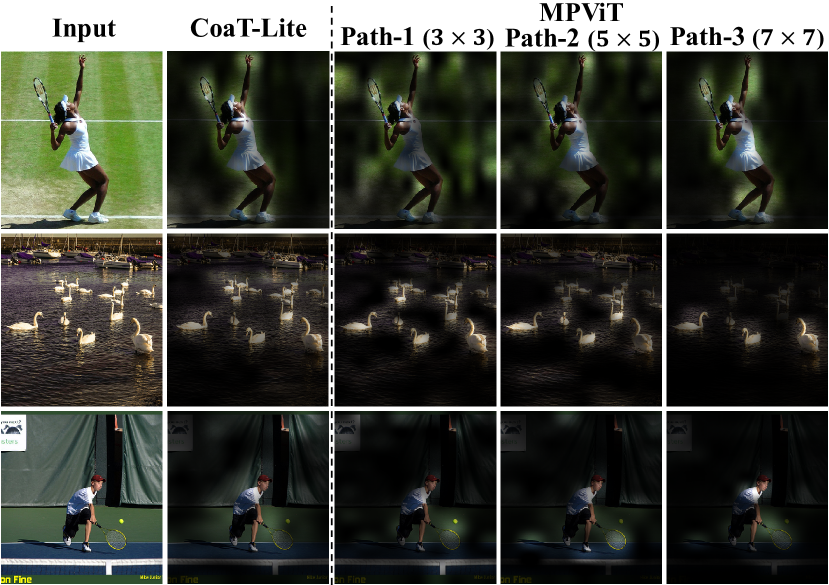
Figure 4: Attention maps generated by CoaT-Lite and MPViT at stage4. MPViT has a triple-path structure with patches of various sizes (e.g., $3\times 3,5\times 5,7\times 7$), leading to fine and coarse features. See Appendix for more visualization results.

Qualitative Analysis

In Fig. 4, we visualize the attention maps, comparing the triple-path (c in Table 5) with the single-path (CoaT-Lite Mini). Since the triple-path embeds different patch sizes, we visualize attention maps for each path. The attention maps from CoaT-Lite and path-1 have similar patch sizes and show similar attention maps. Interestingly, we observe that attention maps from path-3, which attends to larger patches with higher-level representations, are more object centric, precisely capturing the extents of the objects, as shown in the rightmost column of Fig. 4. However, at the same time, path-3 suppresses small objects and noise. Contrarily, path-1 attends to small objects due to fine patches, but does not precisely capture large-object boundaries due to its usage of low-level representations. This is especially apparent in the 3rd-row of Fig. 4, where path-1 captures a smaller ball, while path-3 attends to a larger person. These results demonstrate that combining fine and coarse features via a multi-path structure can capture objects of varying scales in the given visual inputs.

Limitation and Future works

The extensive experimental results have demonstrated that MPViT significantly outperforms current SOTA Vision Transformers not only on image-level prediction, but also on dense predictions tasks. A possible limitation of our MPViT model is the latency at inference time. As shown in Table 7, the inference time of MPViT-S is slower than Swin-T and XCiT-S12/16. We hypothesize that the multi-path structure leads to suboptimal GPU utilization as similar observations have been made for grouped convolution  [64, 40, 32] (e.g., GPU context switching, kernel synchronization, etc.). To alleviate this issue, we are currently working on an efficient implementation of our model to speed-up the inference of MPViT, which integrates the features with different scales into one tensor and then performing multi-head self attention with the tensor. This will improve parallelization and GPU utilization. Moreover, to strike the balanced tradeoff between accuracy/speed, we will further consider path dimensions in a compound scaling strategy [49, 15], to consider the optimal combination of depths, widths, and resolutions when increasing/decreasing the model capacity.

6 Acknowledgement

This work was supported by Institute of Information & Communications Technology Planning & Evaluation (IITP) grant funded by the Korean government (MSIT) (No. 2020-0-00004, Development of Previsional Intelligence based on Long-term Visual Memory Network and No. 2014-3-00123, Development of High Performance Visual BigData Discovery Platform for Large-Scale Realtime Data Analysis).

Appendix A Appendix

In this appendix, Section A.1 first describe the training details of our experiments for ImageNet classification, COCO detection/instance segmentation, and ADE20K semantic segmentation. Second, in Section A.2, we show further experimental analyses for ImageNet classification and COCO object detection. Finally, in Section A.3, we provide more qualitative analysis on the learned attention maps and failure cases.

A.1 Detailed Experimental Settings

ImageNet classification

Following the training recipe as in CoaT [65] and DeiT [14], we perform the same data augmentations such as MixUP [28], CutMix [70], random erasing [72], repeated augmentation [24], and label smoothing [48]. We train MPViTs for 300 epochs with the AdamW [38] optimizer, a batch size of 1024, weight decay of 0.05, five warm-up epochs, and an initial learning rate of 0.001, which is scaled by a cosine decay learning rate scheduler. We implement MPViTs based on CoaT official code  and timm library [59].

Model Param.(M) GFLOPs Top-1 Reference DeiT-T [50]   5.7   1.3 72.2 ICML21 TnT-Ti [21]   6.1   1.4 73.9 NeurIPS21 ViL-Ti-RPB [71]   6.7   1.3 76.7 ICCV21 XCiT-T12/16 [17]   7.0   1.2 77.1 NeurIPS21 ViTAE-6M [66]   6.5   2.0 77.9 NeurIPS21 whitesmokeCoaT-Lite T [65]   5.7   1.6 76.6 ICCV21 powderblueMPViT-T   5.8   1.6 78.2 (+1.6) ResNet-18 [23] 11.7   1.8 69.8 CVPR16 PVT-T [58] 13.2   1.9 75.1 ICCV21 XCiT-T24/16 [17] 12.0   2.3 79.4 NeurIPS21 CoaT Mi [65] 10.0   6.8 80.8 ICCV21 whitesmokeCoaT-Lite Mi [65] 11.0   2.0 78.9 ICCV21 powderblueMPViT-XS 10.5   2.9 80.9 (+2.0) ResNet-50 [23] 25.6   4.1 76.1 CVPR16 PVT-S [58] 24.5   3.8 79.8 ICCV21 DeiT-S/16 [50] 22.1   4.6 79.9 ICML21 Swin-T [37] 29.0   4.5 81.3 ICCV21 Twins-SVT-S [10] 24.0 2.8 81.3 NeurIPS21 TnT-S [21] 23.8   5.2 81.5 NeurIPS21 CvT-13 [60] 20.0   4.5 81.6 ICCV21 XCiT-S12/16 [17] 26.0   4.8 82.0 NeurIPS21 ViTAE-S [66] 23.6   5.6 82.0 NeurIPS21 GG-T [68] 28.0   4.5 82.0 NeurIPS21 CoaT S [65] 22.0 12.6 82.1 ICCV21 Focal-T [67] 29.1   4.9 82.2 NeurIPS21 CrossViT-15 [6] 28.2   6.1 82.3 ICCV21 ViL-S-RPB [71] 24.6   4.9 82.4 ICCV21 CvT-21 [60] 32.0   7.1 82.5 ICCV21 CrossViT-18 [6] 43.3   9.5 82.8 ICCV21 HRFormer-B [69] 50.3 13.7 82.8 NeurIPS21 whitesmokeCoaT-Lite S [65] 20.0   4.0 81.9 ICCV21 powderblueMPViT-S 22.8   4.7 83.0 (+1.1) ResNeXt-101 [64] 83.5 15.6 79.6 CVPR17 PVT-L [58] 61.4   9.8 81.7 ICCV21 DeiT-B/16 [50] 86.6 17.6 81.8 ICML21 XCiT-M24/16 [17] 84.0 16.2 82.7 NeurIPS21 Twins-SVT-B [10] 56.0   8.3 83.1 NeurIPS21 Swin-S [37] 49.6   8.7 83.1 ICCV21 Twins-SVT-L [10] 99.2 14.8 83.3 NeurIPS21 Swin-B [37] 88.0 15.4 83.3 ICCV21 XCiT-S12/8 [17] 26.0 18.9 83.4 NeurIPS21 Focal-S [67] 51.1  9.1 83.5 NeurIPS21 XCiT-M24/8 [17] 84.0 63.9 83.7 NeurIPS21 Focal-B [67] 89.8 16.0 83.8 NeurIPS21 XCiT-S24/8 [17] 48.0 36.0 83.9 NeurIPS21 powderblueMPViT-B 74.8 16.4 84.3

Table 8: Full comparison on ImageNet-1K classification. These models are trained with $224\times 224$ resolution. For fair comparison, we do not include models that are distilled [50] or use $384\times 384$ resolution. Note that CoaT-Lite [65] models are our single-path baselines.

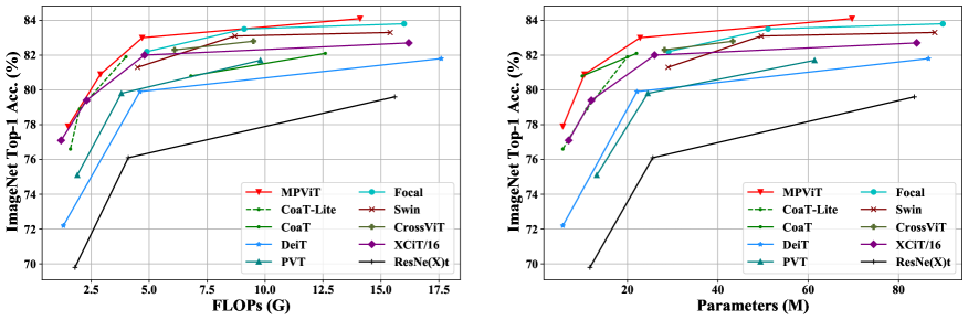
Figure 5: Performance comparisons with respect to FLOPs and model parameters on ImageNet-1K classification. These models are trained with $224\times 224$ single-crop. For fair comparison, we do not include models that are distilled [50] or use $384\times 384$ resolution.

Object detection and Instance segmentation

For fair comparison, we follow the training recipe as in CoaT [65] and Swin Transformer [37] for RetinaNet [35] and Mask R-CNN [22]. Specifically, we train all models for $3\times$ schedule (36 epochs) [22, 61] with multi-scale inputs (MS) [5, 45] which resizes the input such that the shorter side is between 480 and 800 while the longer side is at most 1333). We use the AdamW [38] optimizer, a weight decay of 0.05, a batch size of 16, and an initial learning rate of 0.0001 which is decayed by $10\times$ at epochs 27 and 33. We set stochastic depth drop rates [27] to 0.1, 0.1, 0.2, and 0.4 for Tiny, XSmall, Small, and Base, respectively. We implement all models based on the detectron2 library [61].

Semantic segmentation

Following the same training recipe as in Swin Transformer [37] and XCiT [17], we deploy UperNet [62] with the AdamW [38] optimizer, a weight decay of 0.01, an initial learning rate of $6\times 10^{-5}$ which is scaled using a linear learning rate decay, and linear warmup of 1,500 iterations. We train models for 160K iterations with a batch size of 16 and an input size of $512\times 512$. We use the same data augmentations as [37, 11], utilizing random horizontal flipping, a random re-scaling ratio in the range [0,5, 2.0] and random photometric distortions. We set stochastic depth drop rates [27] to 0.2 and 0.4 for Small and Base, respectively. We implement all models based on the mmseg library [11].

Backbone $AP$ $AP_{50}$ $AP_{75}$ $AP_{S}$ $AP_{M}$ $AP_{L}$ ResNet-50 [23] 44.5 63.7 48.7 26.8 47.6 59.6 CoaT-Lite small [65] 47.0 66.5 51.2 28.8 50.3 63.3 CoaT Small [65] 48.4 68.5 52.4 30.2 51.8 63.8 powderblueMPViT-Small 49.0 68.7 53.7 31.7 52.4 64.5

Table 9: COCO Object Detection results on Deformable DETR [74]. These all models are trained using the same codebase.

A.2 More Experimental Analysis

ImageNet classification

We provide a full summary of comparisons on ImageNet-1K classification in Table 8 by adding more recent Vision Transformers including ViL [71], TnT [21], ViTAE [66], HRFormer [69], and Twins [10]. We can observe that MPViTs consistently achieve state-the-art performance compared to SOTA models with similar model capacity. Notably, the smaller MPViT variants often outperform their larger baseline counterparts even when the baselines use significantly more parameters, as shown in Table 8 and Fig. 5 (right). Furthermore, Fig. 5 demonstrates that MPViT is a more efficient and effective Vision Transformer architecture in terms of computation and model parameters.

Deformable-DETR

Additionally, we compare our MPViT-Small with baselines, CoaT-Lite Small [65] and CoaT Small [65], on the Deformable DETR (DD) [74]. For fair comparison, we train MPViT for 50 epochs with the same training recipe as in CoaT [65]. We use the AdamW [38] optimizer with a batch size of 16, a weight decay of $10^{-4}$, and an initial learning rate of $2\times 10^{-4}$, which is decayed by a factor of 10 at 40 epoch. Tab. 9 shows results comparing with CoaT-Lite Small and CoaT Small. MPViT-Small improves over both CoaT-Lite Small and CoaT Small. Notably, MPViT achieves a larger gain in small object AP (1.5% $AP_{S}$) as compared to others (i.e., $AP_{M}$ or $AP_{L}$).

  Backbone Params. (M) GFLOPs Mask R-CNN $1\times$ RetinaNet $1\times$ $AP^{b}$ $AP^{b}_{50}$ $AP^{b}_{75}$ $AP^{m}$ $AP^{m}_{50}$ $AP^{m}_{75}$ $AP^{b}$ $AP^{b}_{50}$ $AP^{b}_{75}$ $AP^{b}_{S}$ $AP^{b}_{M}$ $AP^{b}_{L}$ PVTv2-B0 [57]   23 (13)   195 (177) 38.2 60.5 40.7 36.2 57.8 38.6 37.2 57.2 39.5 23.1 40.4 49.7 powderblue MPViT-T   28 (17)   216 (196) 42.2 64.2 45.8 39.0 61.4 41.8 41.8 62.7 44.6 27.2 45.1 54.2 PVT-T [58]   33 (23)   240 (221) 39.8 62.2 43.0 37.4 59.3 39.9 39.4 59.8 42.0 25.5 42.0 52.1 PVTv2-B1 [57]   33 (23)   243 (225) 41.8 54.3 45.9 38.8 61.2 41.6 41.2 61.9 43.9 25.4 44.5 54.3 powderblue MPViT-XS   30 (20)   231 (211) 44.2 66.7 48.4 40.4 63.4 43.4 43.8 65.0 47.1 28.1 47.6 56.5 ResNet-50 [23]   44 (38)   260 (239) 38.0 58.6 41.4 34.4 55.1 36.7 36.3 55.3 38.6 19.3 40.4 48.8 PVT-S [58]   44 (34)   305 (226) 43.0 65.3 46.9 39.9 62.5 42.8 42.2 62.7 45.0 26.2 45.2 57.2 PVTv2-B2 [57]   45 (35)   309 (290) 45.3 67.1 49.6 41.2 64.2 44.4 44.6 65.6 47.6 27.4 48.8 58.6 Swin-T [37]   48 (39)   267 (245) 43.7 66.6 47.7 39.8 63.3 42.7 42.0 63.0 44.7 26.6 45.8 55.7 Focal-T [67]   49 (39)   291 (265) 44.8 67.7 49.2 41.0 64.7 44.2 43.7 65.2 46.7 28.6 47.4 56.9 powderblue MPViT-S   43 (32)   268 (248) 46.4 68.6 51.2 42.4 65.6 45.7 45.7 57.3 48.8 28.7 49.7 59.2 ResNeXt101-64x4d [64]  102 (96)   493 (473) 42.8 63.8 47.3 38.4 60.6 41.3 41.0 60.9 44.0 23.9 45.2 54.0 PVT-M [58]   64 (54)   392 (283) 42.0 64.4 45.6 39.0 61.6 42.1 41.9 63.1 44.3 25.0 44.9 57.6 PVT-L [58]   81 (71)   494 (345) 42.9 65.0 46.6 39.5 61.9 42.5 42.6 63.7 45.4 25.8 46.0 58.4 PVTv2-B5 [57]  101 (91)   557 (538) 47.4 68.6 51.9 42.5 65.7 46.0 46.2 67.1 49.5 28.5 50.0 62.5 Swin-S [37]   69 (60)   359 (335) 46.5 68.7 51.3 42.1 65.8 45.2 45.0 66.2 48.3 27.9 48.8 59.5 Swin-B [37]  107 (98)   496 (477) 46.9 69.2 51.6 42.3 66.0 45.5 45.0 66.4 48.3 28.4 49.1 60.6 Focal-S [67]   71 (62)   401 (367) 47.4 69.8 51.9 42.8 66.6 46.1 45.6 67.0 48.7 29.5 49.5 60.3 Focal-B [67]   110 (101)   533 (514) 47.8 70.2 52.5 43.2 67.3 46.5 46.3 68.0 49.8 31.7 50.4 60.8 powderblue MPViT-B   95 (85)   503 (482) 48.2 70.0 52.9 43.5 67.1 46.8 47.0 68.4 50.8 29.4 51.3 61.5

Table 10: COCO detection and instance segmentation with RetinaNet [35] and Mask R-CNN [22]. Models are trained for $1\times$ schedule [61] with single-scale training inputs. All backbones are pretrained on ImageNet-1K. We omit models pretrained on larger-datasets (e.g., ImageNet-21K). The GFLOPs are measured at resolution $800\times 1280$. Mask R-CNN’s parameters/FLOPs are followed by RetinaNet in parentheses.

COCO with $1\times$ schedule.

In addition to the $3\times$ schedule + multi-scale (MS) setting, we also evaluate MPViT on RetinaNet [35] and Mask R-CNN [22] with $1\times$ schedule (12 epochs) [61] using single-scale inputs. Tab. 10 shows result comparisons with state-of-the-art methods. In the results of $3\times$ schedule + multi-scale (MS), we can also observe that MPViTs consistently outperform on both RetinaNet and Mask R-CNN. We note that MPViTs surpass the most recent improved PVTv2 [57] models.

A.3 More Qualitative Results

Visualization of Attention Maps

As shown in Eq.(4), the factorized self-attention in [65] first extracts channel-wise attention softmax$(K)$ by applying a softmax over spatial dimensions (x, y). Then, softmax$(K)^{T}V$ is computed as below:

$$\begin{split}&(\text{softmax}(K)^{T}V)(c_{i},c_{j})\\ &=\sum_{(x,y)}\text{softmax}(K)(x,y,c_{i})V(x,y,c_{j}),\end{split}$$ (5)

where $x$ and $y$ are position of tokens. $c_{i}$ and $c_{j}$ indicate channel indices of $K$ and $V$, respectively. It can be interpreted as multiplying $V$ by the channel-wise spatial attention in a pixel-wise manner followed by the sum over spatial dimension. In other words, softmax$(K)^{T}V$ represents the weighted sum of V where the weight of each position $(x,y)$ is the channel-wise spatial attention. Therefore, to obtain the importance of each position, we employ the mean of softmax$(K)$ over the channel dimension, resulting in spatial attention. Then, the spatial attention is overlaid to the original input image for better visualization, as shown in Fig. 6. In detail, we resize the spatial attention to the size of the original image, normalize the value to [0,1], and then multiply the attention map by the image.

To validate the effectiveness of our attention map qualitatively, we compare attention maps of MPViT and CoaT-Lite [65] in Fig. 6. We compare the attention maps of each method generated from the 4th stage in the same way. For a fair comparison, we pick the best qualitative attention map of each method since both CoaT-Lite and MPViT have eight heads for each layer. Furthermore, we visualize attention maps extracted from all three paths of MPViT to observe the individual effects of each path.

As mentioned in Section 5, the three paths of MPViT can capture objects of varying sizes due to the multi-scale embedding of MPViT as the similar effect of multiple receptive fields. In other words, path-1 concentrates on small objects or textures while path-3 focuses on large objects or high-level semantic concepts. We support this intuition by observing more examples shown in Fig. 6. Attention maps of path-1 (3rd column) capture small objects such as small ducks (4th row), an orange (5th row), a small ball (6th row), and an antelope (8th row). In addition, since path-1 also captures textures due to a smaller receptive field, a relatively low level of attention is present in the background. In contrast, we can observe different behavior for path-3, which can be seen in the rightmost column. Path-3 accentuates large objects while suppressing the background and smaller objects. For example, the ducks (4th row), orange (5th row), and ball (8th row) are masked out in the rightmost column since path-3 concentrates on larger objects. The attention maps of path-2 (4th column) showcase the changing behavior between paths-1 and 3 since the scale of path-2 is in-between the scales of paths-1 and 3, and accordingly, the attention maps also begin to transition from smaller to larger objects. In other words, although the attention map of path-2 attends similar regions as path-1, it is also more likely to emphasize larger objects, as path-3 does. For example, in the last row, path-2 attends to similar regions as path-1 while emphasizing the large giraffes more than path-1. Therefore, although the three paths independently deal with different scales, they act in a complementary manner, which is beneficial for dense prediction tasks.

Since Coat-Lite has a single-path architecture, the singular path needs to deal with objects of varying sizes. Therefore, attention maps from CoaT-Lite (2nd column) simultaneously attend to large and small objects, as shown in the 4th row. However, it is difficult to capture all objects with a single path, as CoaT-Lite misses the orange (5th row) and ball (7th row). In addition, Coat-Lite cannot capture object boundaries as precisely as path-3 of MPViT since path-3 need not attend to small objects or textures. As a result, MPViT shows superior results compared to Coat-Lite on classification, detection, and segmentation tasks.

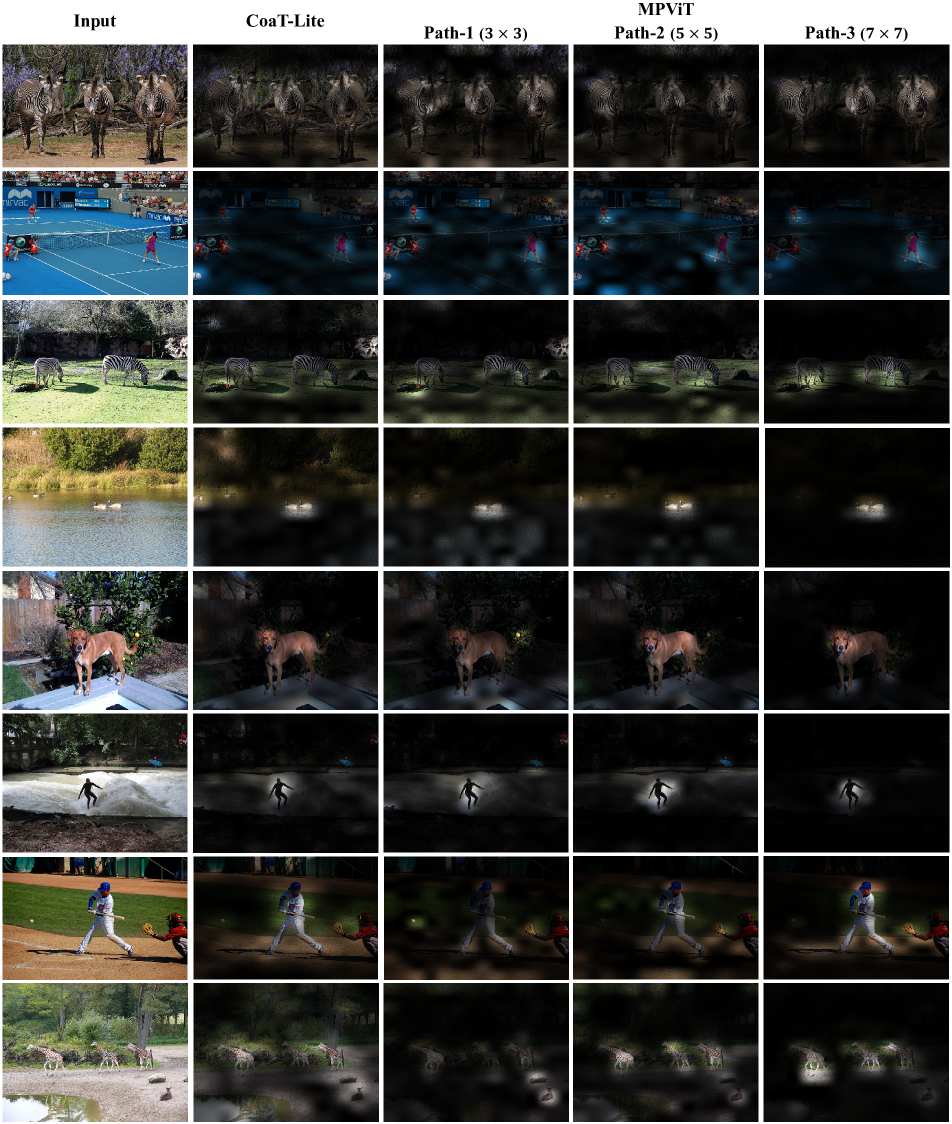
Figure 6: Additional Attention Maps generated by CoaT-Lite [65] and our MPViT. MPViT has a triple-path structure with patches of various sizes (e.g., $3\times 3,5\times 5,7\times 7$), leading to fine and coarse features.

Failure case

In order to verify the effects of attention from a different perspective, we further analyze failure cases on the ImageNet validation images. We show attention maps of each path corresponding to the input image along with the ground truth and the predicted labels of MPViT in Fig. 7. For example, in the first row, the ground truth of the input image is a forklift, while the predicted label is a trailer truck. Although the attention map from path-1 places light emphasis on the forklift, the attention maps from all paths commonly accentuate the trailer truck rather than the forklift, which leads to classifying the image as a trailer truck and not a forklift. Other classification results in Fig. 7 fail in similar circumstances, except for the last row. In the last row, MPViTs attention maps correctly capture the beer bottle. However, the attention maps also attend to the face near the bottle. Therefore, the bottle is misunderstood as a microphone since the image of “drinking a bottle of beer” and “using a microphone” are semantically similar. From the above, we can observe that the attention maps and the predicted results are highly correlated.

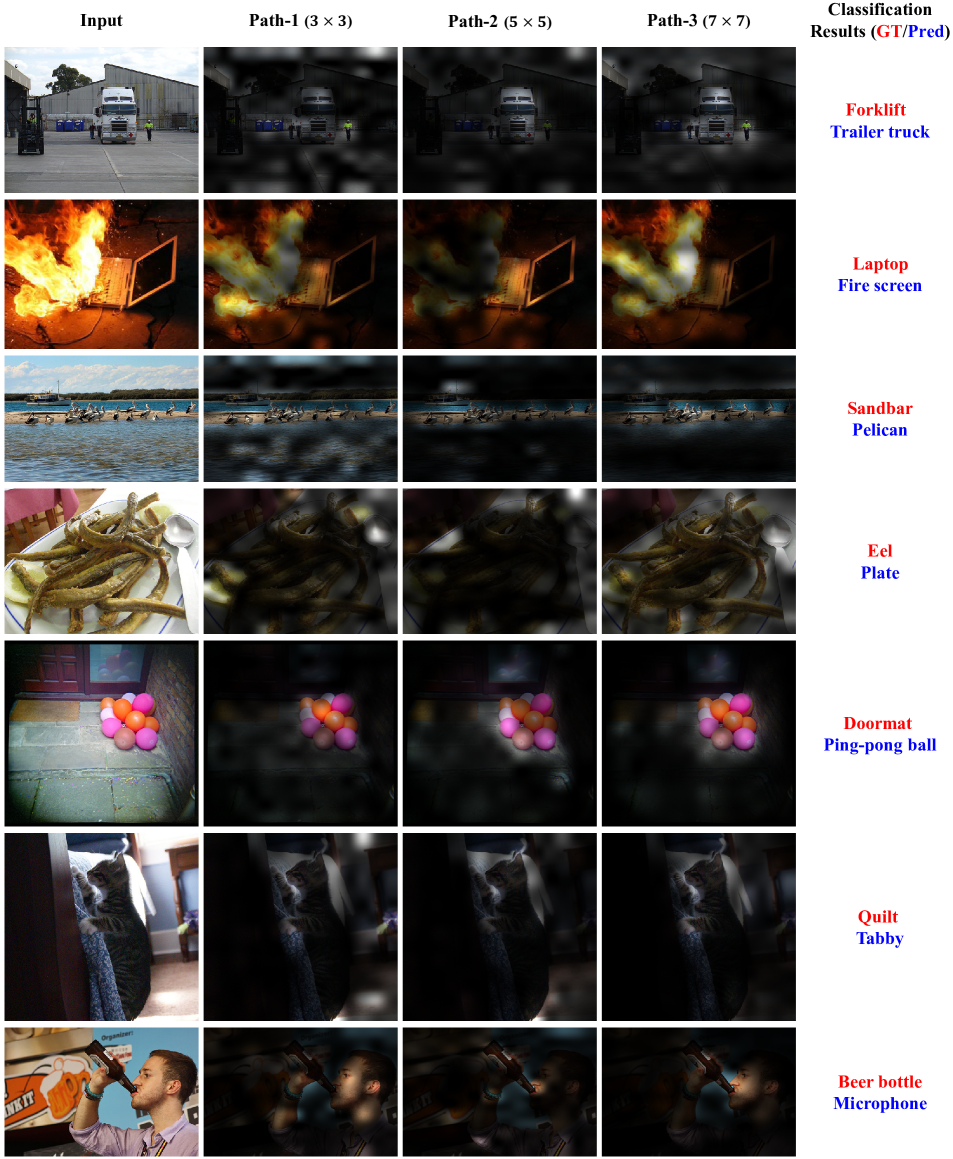
Figure 7: Attention Maps of failure cases on ImageNet validation images. The input image and corresponding attention maps from each path are illustrated. In the rightmost column, we show the ground truth labels and predicted labels colored with red and blue, respectively.

References

- [1] Anurag Arnab, Mostafa Dehghani, Georg Heigold, Chen Sun, Mario Lučić, and Cordelia Schmid. Vivit: A video vision transformer. In ICCV, 2021.
- [2] Nicholas Baker, Hongjing Lu, Gennady Erlikhman, and Philip J Kellman. Deep convolutional networks do not classify based on global object shape. PLoS computational biology, 14(12):e1006613, 2018.
- [3] Gedas Bertasius, Heng Wang, and Lorenzo Torresani. Is space-time attention all you need for video understanding? In ICML, 2021.
- [4] Tom B Brown, Benjamin Mann, Nick Ryder, Melanie Subbiah, Jared Kaplan, Prafulla Dhariwal, Arvind Neelakantan, Pranav Shyam, Girish Sastry, Amanda Askell, et al. Language models are few-shot learners. arXiv preprint arXiv:2005.14165, 2020.
- [5] Nicolas Carion, Francisco Massa, Gabriel Synnaeve, Nicolas Usunier, Alexander Kirillov, and Sergey Zagoruyko. End-to-end object detection with transformers. In ECCV, 2020.
- [6] Chun-Fu Chen, Quanfu Fan, and Rameswar Panda. Crossvit: Cross-attention multi-scale vision transformer for image classification. In ICCV, 2021.
- [7] Xin Chen, Bin Yan, Jiawen Zhu, Dong Wang, Xiaoyun Yang, and Huchuan Lu. Transformer tracking. In CVPR, 2021.
- [8] Zhengsu Chen, Lingxi Xie, Jianwei Niu, Xuefeng Liu, Longhui Wei, and Qi Tian. Visformer: The vision-friendly transformer. In ICCV, 2021.
- [9] François Chollet. Xception: Deep learning with depthwise separable convolutions. In CVPR, 2017.
- [10] Xiangxiang Chu, Zhi Tian, Yuqing Wang, Bo Zhang, Haibing Ren, Xiaolin Wei, Huaxia Xia, and Chunhua Shen. Twins: Revisiting the design of spatial attention in vision transformers. In NeurIPS, 2021.
- [11] MMSegmentation Contributors. MMSegmentation: Openmmlab semantic segmentation toolbox and benchmark. https://github.com/open-mmlab/mmsegmentation, 2020.
- [12] Zhigang Dai, Bolun Cai, Yugeng Lin, and Junying Chen. Up-detr: Unsupervised pre-training for object detection with transformers. In CVPR, 2021.
- [13] Jia Deng, Wei Dong, Richard Socher, Li-Jia Li, Kai Li, and Li Fei-Fei. Imagenet: A large-scale hierarchical image database. In CVPR, 2009.
- [14] Jacob Devlin, Ming-Wei Chang, Kenton Lee, and Kristina Toutanova. Bert: Pre-training of deep bidirectional transformers for language understanding. In NAACL-HLT (1), 2019.
- [15] Piotr Dollár, Mannat Singh, and Ross Girshick. Fast and accurate model scaling. In CVPR, 2021.
- [16] Alexey Dosovitskiy, Lucas Beyer, Alexander Kolesnikov, Dirk Weissenborn, Xiaohua Zhai, Thomas Unterthiner, Mostafa Dehghani, Matthias Minderer, Georg Heigold, Sylvain Gelly, et al. An image is worth 16x16 words: Transformers for image recognition at scale. In ICLR, 2021.
- [17] Alaaeldin El-Nouby, Hugo Touvron, Mathilde Caron, Piotr Bojanowski, Matthijs Douze, Armand Joulin, Ivan Laptev, Natalia Neverova, Gabriel Synnaeve, Jakob Verbeek, et al. Xcit: Cross-covariance image transformers. In NeurIPS, 2021.
- [18] Haoqi Fan, Bo Xiong, Karttikeya Mangalam, Yanghao Li, Zhicheng Yan, Jitendra Malik, and Christoph Feichtenhofer. Multiscale vision transformers. In ICCV, 2021.
- [19] Shanghua Gao, Ming-Ming Cheng, Kai Zhao, Xin-Yu Zhang, Ming-Hsuan Yang, and Philip HS Torr. Res2net: A new multi-scale backbone architecture. TPAMI, 2019.
- [20] Ben Graham, Alaaeldin El-Nouby, Hugo Touvron, Pierre Stock, Armand Joulin, Hervé Jégou, and Matthijs Douze. Levit: a vision transformer in convnet’s clothing for faster inference. In ICCV, 2021.
- [21] Kai Han, An Xiao, Enhua Wu, Jianyuan Guo, Chunjing Xu, and Yunhe Wang. Transformer in transformer. In NeurIPS, 2021.
- [22] Kaiming He, Georgia Gkioxari, Piotr Dollár, and Ross Girshick. Mask r-cnn. In CVPR, 2017.
- [23] Kaiming He, Xiangyu Zhang, Shaoqing Ren, and Jian Sun. Deep residual learning for image recognition. In CVPR, 2016.
- [24] Elad Hoffer, Tal Ben-Nun, Itay Hubara, Niv Giladi, Torsten Hoefler, and Daniel Soudry. Augment your batch: Improving generalization through instance repetition. In CVPR, 2020.
- [25] Andrew Howard, Mark Sandler, Grace Chu, Liang-Chieh Chen, Bo Chen, Mingxing Tan, Weijun Wang, Yukun Zhu, Ruoming Pang, Vijay Vasudevan, et al. Searching for mobilenetv3. In CVPR, 2019.
- [26] Andrew G Howard, Menglong Zhu, Bo Chen, Dmitry Kalenichenko, Weijun Wang, Tobias Weyand, Marco Andreetto, and Hartwig Adam. Mobilenets: Efficient convolutional neural networks for mobile vision applications. arXiv preprint arXiv:1704.04861, 2017.
- [27] Gao Huang, Yu Sun, Zhuang Liu, Daniel Sedra, and Kilian Q Weinberger. Deep networks with stochastic depth. In ECCV, 2016.
- [28] Hiroshi Inoue. Data augmentation by pairing samples for images classification. arXiv preprint arXiv:1801.02929, 2018.
- [29] Sergey Ioffe and Christian Szegedy. Batch normalization: Accelerating deep network training by reducing internal covariate shift. In ICML, 2015.
- [30] Md Amirul Islam, Sen Jia, and Neil DB Bruce. How much position information do convolutional neural networks encode? arXiv preprint arXiv:2001.08248, 2020.
- [31] Osman Semih Kayhan and Jan C van Gemert. On translation invariance in cnns: Convolutional layers can exploit absolute spatial location. In CVPR, 2020.
- [32] Youngwan Lee, Joong-won Hwang, Sangrok Lee, Yuseok Bae, and Jongyoul Park. An energy and gpu-computation efficient backbone network for real-time object detection. In CVPRW, 2019.
- [33] Youngwan Lee, Huieun Kim, Eunsoo Park, Xuenan Cui, and Hakil Kim. Wide-residual-inception networks for real-time object detection. In IEEE Intelligent Vehicles Symposium (IV), 2017.
- [34] Tsung-Yi Lin, Piotr Dollár, Ross Girshick, Kaiming He, Bharath Hariharan, and Serge Belongie. Feature pyramid networks for object detection. In CVPR, 2017.
- [35] Tsung-Yi Lin, Priya Goyal, Ross Girshick, Kaiming He, and Piotr Dollár. Focal loss for dense object detection. In ICCV, 2017.
- [36] Tsung-Yi Lin, Michael Maire, Serge Belongie, James Hays, Pietro Perona, Deva Ramanan, Piotr Dollár, and C Lawrence Zitnick. Microsoft coco: Common objects in context. In ECCV, 2014.
- [37] Ze Liu, Yutong Lin, Yue Cao, Han Hu, Yixuan Wei, Zheng Zhang, Stephen Lin, and Baining Guo. Swin transformer: Hierarchical vision transformer using shifted windows. In ICCV, 2021.
- [38] Ilya Loshchilov and Frank Hutter. Decoupled weight decay regularization. arXiv preprint arXiv:1711.05101, 2017.
- [39] David G Lowe. Object recognition from local scale-invariant features. In ICCV, 1999.
- [40] Ningning Ma, Xiangyu Zhang, Hai-Tao Zheng, and Jian Sun. Shufflenet v2: Practical guidelines for efficient cnn architecture design. In ECCV, 2018.
- [41] Tim Meinhardt, Alexander Kirillov, Laura Leal-Taixe, and Christoph Feichtenhofer. Trackformer: Multi-object tracking with transformers. arXiv preprint arXiv:2101.02702, 2021.
- [42] Alejandro Newell, Kaiyu Yang, and Jia Deng. Stacked hourglass networks for human pose estimation. In ECCV, 2016.
- [43] Alec Radford, Karthik Narasimhan, Tim Salimans, and Ilya Sutskever. Improving language understanding with unsupervised learning. Technical report, OpenAI, 2018.
- [44] Karen Simonyan and Andrew Zisserman. Very deep convolutional networks for large-scale image recognition. In ICLR, 2014.
- [45] Peize Sun, Rufeng Zhang, Yi Jiang, Tao Kong, Chenfeng Xu, Wei Zhan, Masayoshi Tomizuka, Lei Li, Zehuan Yuan, Changhu Wang, et al. Sparse r-cnn: End-to-end object detection with learnable proposals. In CVPR, 2021.
- [46] Christian Szegedy, Sergey Ioffe, Vincent Vanhoucke, and Alexander A Alemi. Inception-v4, inception-resnet and the impact of residual connections on learning. In AAAI, 2017.
- [47] Christian Szegedy, Wei Liu, Yangqing Jia, Pierre Sermanet, Scott Reed, Dragomir Anguelov, Dumitru Erhan, Vincent Vanhoucke, and Andrew Rabinovich. Going deeper with convolutions. In CVPR, 2015.
- [48] Christian Szegedy, Vincent Vanhoucke, Sergey Ioffe, Jon Shlens, and Zbigniew Wojna. Rethinking the inception architecture for computer vision. In CVPR, 2016.
- [49] Mingxing Tan and Quoc Le. Efficientnet: Rethinking model scaling for convolutional neural networks. In ICML, 2019.
- [50] Hugo Touvron, Matthieu Cord, Matthijs Douze, Francisco Massa, Alexandre Sablayrolles, and Hervé Jégou. Training data-efficient image transformers & distillation through attention. In ICML, 2021.
- [51] Hugo Touvron, Matthieu Cord, Alexandre Sablayrolles, Gabriel Synnaeve, and Hervé Jégou. Going deeper with image transformers. In ICCV, 2021.
- [52] Shikhar Tuli, Ishita Dasgupta, Erin Grant, and Thomas L Griffiths. Are convolutional neural networks or transformers more like human vision? arXiv preprint arXiv:2105.07197, 2021.
- [53] Ashish Vaswani, Noam Shazeer, Niki Parmar, Jakob Uszkoreit, Llion Jones, Aidan N Gomez, Łukasz Kaiser, and Illia Polosukhin. Attention is all you need. In NeurIPS, 2017.
- [54] Huiyu Wang, Yukun Zhu, Hartwig Adam, Alan Yuille, and Liang-Chieh Chen. Max-deeplab: End-to-end panoptic segmentation with mask transformers. In CVPR, 2021.
- [55] Jingdong Wang, Ke Sun, Tianheng Cheng, Borui Jiang, Chaorui Deng, Yang Zhao, Dong Liu, Yadong Mu, Mingkui Tan, Xinggang Wang, et al. Deep high-resolution representation learning for visual recognition. TPAMI, 2020.
- [56] Ning Wang, Wengang Zhou, Jie Wang, and Houqiang Li. Transformer meets tracker: Exploiting temporal context for robust visual tracking. In ICCV, 2021.
- [57] Wenhai Wang, Enze Xie, Xiang Li, Deng-Ping Fan, Kaitao Song, Ding Liang, Tong Lu, Ping Luo, and Ling Shao. Pvtv2: Improved baselines with pyramid vision transformer. arXiv preprint arXiv:2106.13797, 2021.
- [58] Wenhai Wang, Enze Xie, Xiang Li, Deng-Ping Fan, Kaitao Song, Ding Liang, Tong Lu, Ping Luo, and Ling Shao. Pyramid vision transformer: A versatile backbone for dense prediction without convolutions. In ICCV, 2021.
- [59] Ross Wightman. Pytorch image models. https://github.com/rwightman/pytorch-image-models, 2019.
- [60] Haiping Wu, Bin Xiao, Noel Codella, Mengchen Liu, Xiyang Dai, Lu Yuan, and Lei Zhang. Cvt: Introducing convolutions to vision transformers. In ICCV, 2021.
- [61] Yuxin Wu, Alexander Kirillov, Francisco Massa, Wan-Yen Lo, and Ross Girshick. Detectron2. https://github.com/facebookresearch/detectron2, 2019.
- [62] Tete Xiao, Yingcheng Liu, Bolei Zhou, Yuning Jiang, and Jian Sun. Unified perceptual parsing for scene understanding. In ECCV, 2018.
- [63] Enze Xie, Wenhai Wang, Zhiding Yu, Anima Anandkumar, Jose M Alvarez, and Ping Luo. Segformer: Simple and efficient design for semantic segmentation with transformers. In NeurIPS, 2021.
- [64] Saining Xie, Ross Girshick, Piotr Dollár, Zhuowen Tu, and Kaiming He. Aggregated residual transformations for deep neural networks. In CVPR, 2017.
- [65] Weijian Xu, Yifan Xu, Tyler Chang, and Zhuowen Tu. Co-scale conv-attentional image transformers. In ICCV, 2021.
- [66] Yufei Xu, Qiming Zhang, Jing Zhang, and Dacheng Tao. Vitae: Vision transformer advanced by exploring intrinsic inductive bias. In NeurIPS, 2021.
- [67] Jianwei Yang, Chunyuan Li, Pengchuan Zhang, Xiyang Dai, Bin Xiao, Lu Yuan, and Jianfeng Gao. Focal self-attention for local-global interactions in vision transformers. In NeurIPS, 2021.
- [68] Qihang Yu, Yingda Xia, Yutong Bai, Yongyi Lu, Alan Yuille, and Wei Shen. Glance-and-gaze vision transformer. In NeurIPS, 2021.
- [69] Yuhui Yuan, Rao Fu, Lang Huang, Weihong Lin, Chao Zhang, Xilin Chen, and Jingdong Wang. Hrformer: High-resolution transformer for dense prediction. In NeurIPS, 2021.
- [70] Sangdoo Yun, Dongyoon Han, Seong Joon Oh, Sanghyuk Chun, Junsuk Choe, and Youngjoon Yoo. Cutmix: Regularization strategy to train strong classifiers with localizable features. In ICCV, 2019.
- [71] Pengchuan Zhang, Xiyang Dai, Jianwei Yang, Bin Xiao, Lu Yuan, Lei Zhang, and Jianfeng Gao. Multi-scale vision longformer: A new vision transformer for high-resolution image encoding. In ICCV, 2021.
- [72] Zhun Zhong, Liang Zheng, Guoliang Kang, Shaozi Li, and Yi Yang. Random erasing data augmentation. In AAAI, 2020.
- [73] Bolei Zhou, Hang Zhao, Xavier Puig, Sanja Fidler, Adela Barriuso, and Antonio Torralba. Scene parsing through ade20k dataset. In CVPR, 2017.
- [74] Xizhou Zhu, Weijie Su, Lewei Lu, Bin Li, Xiaogang Wang, and Jifeng Dai. Deformable detr: Deformable transformers for end-to-end object detection. In ICLR, 2021.