Efficient Quantum Network Communication using Optimized Entanglement-Swapping Trees

Abstract

Quantum network communication is challenging, as the No-cloning theorem in quantum regime makes many classical techniques inapplicable. For long-distance communication, the only viable communication approach is teleportation of quantum states, which requires a prior distribution of entangled pairs (EPs) of qubits. Establishment of EPs across remote nodes can incur significant latency due to the low probability of success of the underlying physical processes.

The focus of our work is to develop efficient techniques that minimize EP generation latency. Prior works have focused on selecting entanglement paths; in contrast, we select entanglement swapping trees—a more accurate representation of the entanglement generation structure. We develop a dynamic programming algorithm to select an optimal swapping-tree for a single pair of nodes, under the given capacity and fidelity constraints. For the general setting, we develop an efficient iterative algorithm to compute a set of swapping trees. We present simulation results which show that our solutions outperform the prior approaches by an order of magnitude and are viable for long-distance entanglement generation.

1 Introduction

Fundamental advances in physical sciences and engineering have led to the realization of working quantum computers (QCs) [1, 20]. However, there are significant limitations to the capacity of individual QC [7]. Quantum Networks (QNs) enable the construction of large, robust, and more capable quantum computing platforms by connecting smaller QCs. Quantum networks [33] also enable various important applications [17, 31, 22, 11, 25]. However, quantum network communication is challenging — e.g., physical transmission of quantum states across nodes can incur irreparable communication errors, as the No-cloning Theorem [15] proscribes making independent copies of arbitrary qubits. At the same time, certain aspects unique to the quantum regime, such as entangled states, enables novel mechanisms for communication. In particular, teleportation [3] transfers quantum states with just classical communication, but requires an a priori establishment of entangled pairs (EPs). This paper presents techniques for efficient establishment of EPs in a network.

Establishment of EPs over long distances is challenging. Coordinated entanglement swapping (e.g. DLCZ protocol [16]) using quantum repeaters can be used to establish long-distance entanglements from short-distance entanglements. However, due to low probability of success of the underlying physical processes (short-distance entanglements and swappings), EP generation can incur significant latency— of the order of 10s to 100s of seconds between nodes 100s of kms away [30]. Thus, we need to develop techniques that can facilitate fast generation of long-distance EPs. We employ two strategies to minimize generation latencies: (i) select optimal swapping trees (not, just paths as in prior works [32, 9, 27, 10]) with a protocol that retains unused EPs; (ii) use multiple trees for each given node pair; this reduces effective latency by using all available network resources. In the above context, we address the following problems: (i) QNR-SP Problem: Given a single $(s,d)$ pair, select a minimum-latency swapping tree under given constraints. (ii) QNR Problem: Given a set of source-destination $(s,d)$ pairs, select a set of swapping trees for each pair with maximum aggregate EP generation rate, under fidelity and resource constraints.

To the best of our knowledge, no prior work has addressed the problem of selecting an efficient swapping-tree for entanglement routing; they all consider selecting routing paths ( [8] selects a path using a metric based on balanced trees; see §3.2). Almost all prior works have considered the “waitless” model, wherein all underlying physical processes much succeed near-simultaneously for an EP to be generated; this model incurs minimal decoherence, but yields very low EP generation rates. In contrast, we consider the “waiting” protocol, wherein, at each swap operation, the earlier arriving EP waits for a limited time for the other EP to be generated. Such an approach with efficient swapping trees yields high entanglement rates; the potential decoherence risk can be handled by discarding qubits that "age" beyond a certain threshold.

Our Contributions. We formulate the entanglement routing problem (§3) in QNs in terms of selecting optimal swapping trees in the “waiting” protocol, under fidelity constraints. In this context, we make the following contributions:

• For the QNR-SP problem, we design an optimal algorithm with fidelity and resource constraints (§4).

• Though polynomial-time, the above optimal algorithm has high time complexity; we thus also design a near-linear time heuristic for the QNR-SP problem based on an appropriate metric which essentially restricts the solutions to balanced swapping trees (§5).

• For the general QNR problem, we design an efficient iterative augmenting-tree algorithm (§6), and show its effectiveness w.r.t. an optimal LP solution based on hypergraph-flows.

• We conduct extensive evaluations (§7) using NetSquid simulator, and show that our solutions outperform the prior approaches by an order of magnitude, while incurring little fidelity degradation. We also show that our schemes can generate high-fidelity EPs over nodes 500-1000kms away.

2 QC Background

Qubit States. Quantum computation manipulates qubits analogous to how classical computation manipulates bits. At any given time, a bit may be in one of two states, traditionally represented by $0$ and $1$. A quantum state represented by a qubit is a superposition of classical states, and is usually written as $\alpha_{0}|0\rangle+\alpha_{1}|1\rangle$, where $\alpha_{0}$ and $\alpha_{1}$ are amplitudes represented by complex numbers and such that $|\alpha_{0}|^{2}+|\alpha_{1}|^{2}=1$. Here, $|0\rangle$ and $|1\rangle$ are the standard (orthonormal) basis states; concretely, they may represent physical properties such as spin (down/up), polarization, charge direction, etc. When a qubit such as above is measured, it collapses to a $|0\rangle$ state with a probability of $|\alpha_{0}|^{2}$ and to a $|1\rangle$ state with a probability of $|\alpha_{1}|^{2}$. In general, a state of an $n$ qubit system can be represented as $\Sigma_{i=0}^{2^{n}-1}\alpha_{i}|i\rangle$ where “$i$” in $|i\rangle$ is $i$’s bit representation.

Entanglement. Entangled states are multi-qubit states that cannot be "factorized" into independent single-qubit states. E.g., the $2$-qubit state $\frac{1}{\sqrt{2}}|00\rangle+\frac{1}{\sqrt{2}}|11\rangle$; this particular system is a maximally-entangled state. We refer to maximally-entangled pairs of qubits as EPs. The surprising aspect of entangled states is that the combined system continues to stay entangled, even when the individual qubits are physically separated by large distances. This facilitates many applications, e.g., teleportation of qubit states by local operations and classical information exchange, as described next.

Teleportation. Quantum data cannot be cloned [39, 15], i.e., it is not possible to make independent copies of arbitrary quantum information. Consequently, direct transmission of quantum data is subject to unrecoverable errors, as classical procedures such as amplified signals or re-transmission cannot be applied. An alternative mechanism for quantum communication is teleportation, Fig. 1 (a), where a qubit $q$ from a node $A$ is recreated in another node $B$ (while “destroying” the original qubit $q$) using only classical communication. However, this process requires that an EP already established over the nodes $A$ and $B$. Teleportation can thus be used to reliably transfer quantum information. At a high-level, the process of teleporting an arbitrary qubit, say qubit $q$, from node $A$ to node $B$ can be summarized as follows:

• an EP pair $(e_{1},e_{2})$ is generated over $A$ and $B$, with $e_{1}$ stored at $A$ and $e_{2}$ stored at $B$;

• at $A$, a Bell-state measurement (BSM) operation over $e_{1}$ and $q$ is performed, and the 2 classical bits measurement output $(c_{1}c_{2})$ is sent to $B$ through the classical communication channel; at this point, the qubits $q$ and $e_{1}$ at $A$ are destroyed.

• manipulating the EP-pair qubit $e_{2}$ at $B$ based on received $(c_{1},c_{2})$ changes its state to $q$’s initial state.

Depending on the physical realization of qubits and the BSM operation, it may not always be possible to successfully generate the 2 classical bits, as the BSM operation is stochastic.

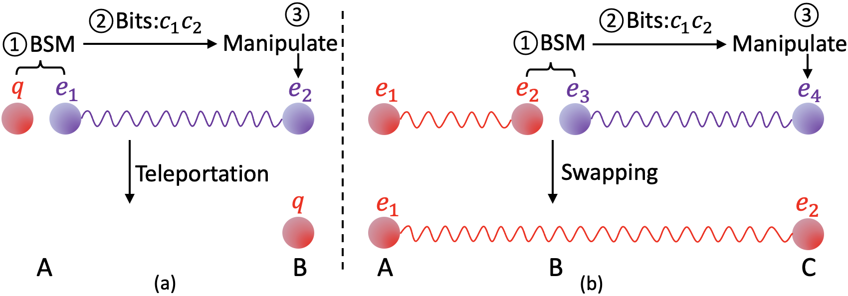
Figure 1: (a) Teleportation of $|q\rangle$ from $A$ to $B$, while consuming an entangled pair $(e_{1},e_{2})$. (b) Entanglement swapping over the triplet of nodes $(A,B,C)$, which results in $A$’s qubit entangled with $C$’s qubit. This can be viewed as a teleportation of $e_{2}$ from node $B$ to $C$.

Entanglement Swapping (ES). Entanglement swapping is an application of teleportation to generate EPs over remote nodes. See Fig. 1 (b). If $A$ and $B$ share an EP and $B$ teleports its qubit to $C$, then $A$ and $C$ end up sharing an EP. More elaborately, let us assume that $A$ and $B$ share an EP, and $B$ and $C$ share a separate EP. Now, $B$ performs a BSM on its two qubits and communicates the result to $C$ (teleporting its qubit that is entangled with $A$ to $C$). When $C$ finishes the protocol, it has a qubit that is an entangled with $A$’s qubit. Thus, an entanglement swapping (ES) operation can be looked up as being performed over a triplet of nodes $(A,B,C)$ with EP available at the two pairs of adjacent nodes $(A,B)$ and $(B,C)$; it results in an EP over the pair of nodes $(A,C)$.

Fidelity: Decoherence and Operations-Driven. Fidelity is a measure of how close a realized state is to the ideal. Fidelity of qubit decreases with time, due to interaction with the environment, as well as gate operations (e.g., in ES). Time-driven fidelity degradation is called decoherence. To bound decoherence, we limit the aggregate time a qubit spends in a quantum memory before being consumed. With regards to operation-driven fidelity degradation, Briegel et al. [6] give an expression that relates the fidelity of an EP generated by ES to the fidelities of the operands, in terms of the noise introduced by swap operations and the number of link EPs used. The order of the swap operations (i.e., the structure of the swapping tree) does not affect the fidelity. Thus, the operation-driven fidelity degradation of the final EP generated by a swapping-tree $T$ can be controlled by limiting the number of leaves of $T$, assuming that the link EPs have uniform fidelity (as in [9]).

Entanglement Purification [6, e.g.] and Quantum Error Correction [28, e.g.] have been widely used to combat fidelity degradation. Our work focuses on optimally scheduling ES operations with constraints on fidelity degradation, without purification or error correction.

2.1 Generating Entanglement Pairs (EPs)

As described above, teleportation, which is the only viable means of transferring quantum states over long distances, requires an a priori distribution of EPs. Thus, we need efficient mechanisms to establish EPs across remote QN nodes; this is the goal of our work. Below, we start with describing how EPs are generated between adjacent (i.e., one-hop away) nodes, and then discuss how EPs across a pair of remote nodes can be established via ESs.

Generating EP over Adjacent Nodes. The physical realization of qubits determines the technique used for sharing EPs between adjacent nodes. The heralded entanglement process [32, 8] to generate an atom-atom EP between adjacent nodes $A$ and $B$ is as follows:

• Generate an entangled pair of atom and a telecom-wavelength photon at node $A$ and $B$. Qubits at each node are generally realized in an atomic form for longer-term storage, while photonic qubits are used for transmission.

• Once an atom-photon entanglement is locally generated at each node (at the same time), the telecom-photons are then transmitted over an optical fiber to a photon-photon/optical BSM device $C$ located in the middle of $A$ and $B$ so that the photons arrive at $C$ at the same time.

• The device $C$ performs a BSM over the photons, and transmits the classical result to $A$ or $B$ to complete ES.

Other entanglement generation processes have been proposed [26]; our techniques themselves are independent of how the link EP are generated.

Generating EP between Remote Nodes. Now, EP between non-adjacent nodes connected by a path in the network can be established by performing a sequence of ESs at intermediate nodes; this requires an a priori EP over each of the adjacent pairs of nodes in the path. E.g., consider a path of nodes $x_{0},x_{1},x_{2},x_{3},x_{4},x_{5}$, with an EP between every pair of adjacent nodes $(x_{i},x_{i+1})$. Thus, each node $x_{i}$ ($1\leq i\leq 4$) has two qubits, one of which is entangled with $x_{i-1}$ and the other with $x_{i+1}$. Nodes $x_{0}$ and $x_{5}$ have only one qubit each. To establish an EP between $x_{0}$ and $x_{5}$, we can perform a sequence of entanglement swappings (ESs) as shown in Fig. 2. Similarly, the sequence of ES over the following triplets would also work: $(x_{2},x_{3},x_{4})$, $(x_{2},x_{4},x_{5})$, $(x_{0},x_{1},x_{2})$, $(x_{0},x_{2},x_{5})$.

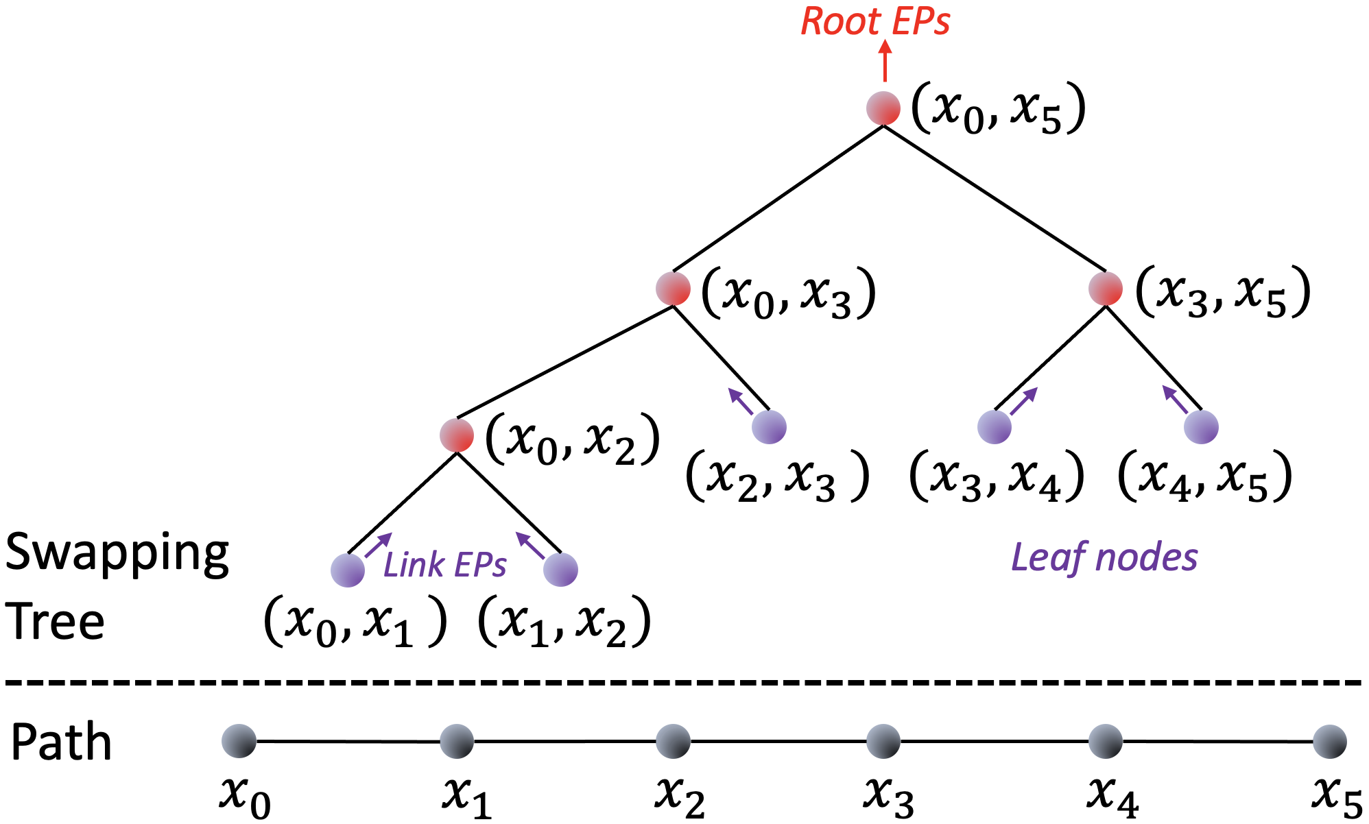
Figure 2: A swapping tree over a path. The leaves of the tree are the path-links, which generate link-EPs continuously.

Swapping Trees. In general, given a path $P=s\leadsto d$ from $s$ to $d$, any complete binary tree (called a swapping tree) over the ordered links in $P$ gives a way to generate an EP over $(s,d)$. Each vertex in the tree corresponds to a pair of network nodes in $P$, with each leaf representing a link in $P$. Every pair of siblings $(A,B)$ and $(B,C)$ perform an ES over $(A,B,C)$ to yield an EP over $(A,C)$—their parent. See Fig. 2. Note that subtrees of a swapping tree execute in parallel. Different swapping trees over the same path $P$ can have different performance characteristics, as discussed later (see Fig. 4).

Expected Generation Latency/Rate of EPs. In general, our goal is to continuously generate EPs at some rate using a swapping tree, using continuously generated EPs at the leaves. The stochastic nature of ES operations means that an EP at the tree’s root will be successfully generated only after many failed attempts and hence significant latency. We refer to this latency as the generation latency of the EP at the root, and in short, just the generation latency of the tree. EP generation rate is the inverse of its generation latency. Whenever we refer to generation latency/rate, we implicitly mean expected generation latency/rate.

Two Generation Protocols: WaitLess and Waiting When a swapping tree is used to (continuously) generate EPs, there are two fundamentally different generation protocols [30, 36].

• WaitLess Protocol. In this model, all the underlying processes, including link EP generations and atomic BSMs are synchronized. If all of them succeed then the end-to-end EP is generated. If any of the underlying processes fail, then all the generated EPs are discarded and the whole process starts again from scratch (from generation of EP at links). In the WaitLess protocol, all swapping trees over a given path $P$ incur the same generation latency—thus, here, the goal is to select an optimal path $P$ (as in [32, 9]).

• Waiting Protocol. In Waiting protocol, a qubit of an EP may wait (in a quantum memory) for its counterpart to become available so that an ES operation can be performed. Using such storage, we preclude discarding successfully generated EPs, and thus, reduce the overall latency in generation of a root-level EP. E.g., let $(A,B)$ and $(B,C)$ be two siblings in a swapping tree and EP for $(A,B)$ is generated first. Then, EP $(A,B)$ may wait for the EP $(B,C)$ to be successfully generated. Once the EP $(B,C)$ is generated, the ES operation is done over the triplet $(A,B,C)$ to generate the EP $(A,C)$. If the EP $(A,C)$ waits beyond a certain threshold, then it may decohere.

Why Waiting is Never Worse. The focus of the WaitLess protocol is to avoid qubit decoherence due to storage. But it results in very low generation rates due to a very-low probability of all the underlying processes succeeding at the same time. However, since qubit coherence times are typically higher than the link-generation latencies, an appropriately designed Waiting protocol will always yield better generation rates without significantly compromising the fidelity (see Theorem 1). The key is to bound the waiting time to limit decoherence as desired; e.g., in our protocol, we restrict to trees with high expected fidelities (§3), and discard qubits that "age" beyond a threshold (§4.2). Both protocols use the same number of quantum memories (2 per node), though the Waiting protocols will benefit from low-decoherence memories; other hardware requirements also remain the same.

Theorem 1

Consider a quantum network, a path $P$, a swapping-tree $T$ over $P$, a WaitLess protocol $X$, and a Waiting protocol $Y$. Protocol $Y$ discards qubits that age (stay in memory) beyond a certain threshold $\tau$ (presumably, equal to the coherence time). We claim that $Y$’s EP generation rate will at least be that of $X$, irrespective of $\tau$ and $T$ (as long as it is over $P$), while ensuring that EPs generated by $Y$ are formed by non-decohered qubits and the operation-driven fidelity degradation of $Y$ EPs is same as $X$.  

The above theorem suggests that Waiting approach is always a better approach, irrespective of the decoherence time/limitations. See proof in Appendix B.

3 Model, Problem, and Related Works

In this section, we discuss our network model, formulate the problem addressed, and discuss related work.

Network Model. We denote a quantum network (QN) with a graph $G=(V,E)$, with $V=\{v_{1},v_{2},\ldots,v_{n}\}$ and $E=\{(v_{i},v_{j})\}$ denoting the set of nodes and links respectively. Pairs of nodes connected by a link are defined as adjacent nodes. We follow the network model in [8] closely. Thus, each node has an atom-photon EP generator with generation latency ($t_{g}$) and probability of success ($p_{g}$). Generation latency is the time between successive attempts by the node to excite the atom to generate an atom-photon EP; this implicitly includes the times for photon transmission, optical-BSM latency, and classical acknowledgement. For clarity of presentation and without loss of generality, we assume homogeneous network nodes with same parameter values. The generation rate is the inverse of generation latency, as before. A node’s atom-photon generation capacity/rate is its aggregate capacity, and may be split across its incident links (i.e., in generation of EPs over its incident links/nodes). Each node is also equipped with a certain number of atomic memories to store the qubits of the atom-atom EPs.

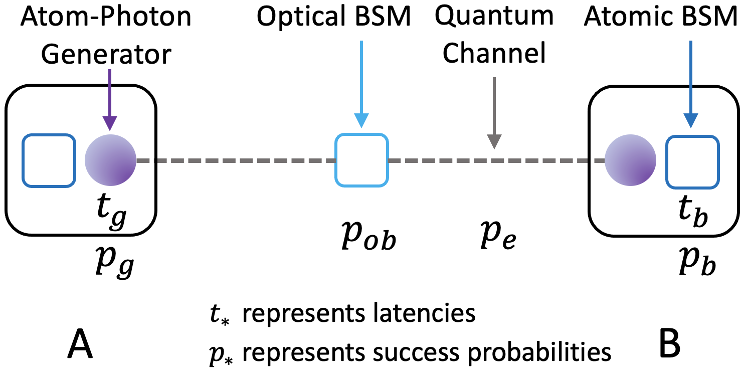
Figure 3: Key notations used.

A network link is a quantum channel (e.g., using an optical fiber or a free-space link), and, in our context, is used only for establishment of link EP. In particular, a link $e=(A,B)$ is used to transmit telecom-photons from $A$ and $B$ to the photon-photon BSM device in the middle of $e$. Thus, each link is composed of two half-links with a probability of transmission success ($p_{e}$) that decreases exponentially with the link distance (see §7). The optical-BSM operation has a certain probability of success ($p_{ob}$). To facilitate atom-atom ES operations, each network node is also equipped with an atomic-BSM device with an operation latency ($t_{b}$) and probability of success ($p_{b}$). Finally, there is an independent classical network with a transmission latency ($t_{c}$); we assume classical transmission always succeeds.

Single vs. Multiple Links Between Nodes. For our techniques multiple links between a pair of adjacent nodes can be replaced by a single link of aggregated rate/capacity. Hence we assume only a single link between every pair of nodes. However, distinct multiple links between nodes have been used creatively in [32] (which refers to them as multiple channels); thus, we will discuss multiple links further in §7 when we evaluate various techniques.

EP Generation Latency of a Swapping Tree. Given a swapping tree and EP generation rates at the leaves (network links), we wish to estimate the generation latency of the EPs over the remote pair corresponding to the tree’s root with the Waiting protocol. Below, we develop a recursive equation. Consider a node $(A,C)$ in the tree, with $(A,B)$ and $(B,C)$ as its two children. Let $T_{AB},T_{BC}$, and $T_{AC}$ be the corresponding (expected) generation latencies of the EPs over the three pairs of nodes. Below, we derive an expression for $T_{AC}$ in terms of $T_{AB}$ and $T_{BC}$; this expression will be sufficient to determine the expected latency of the overall swapping tree by applying the expression iteratively. We start with an observation.

Observation 1

If two EP arrival processes $X_{1}$ and $X_{2}$ are exponentially distributed with a mean inter-arrival latency of $\lambda$ each, then the expected inter-arrival latency of $\max(X,Y)$ is $(3/2)\lambda$.

From above, if assume $T_{AB}$ and $T_{BC}$ to be exponentially distributed with the same expected generation latency of $T$, then the expected latency of both EPs arriving is $(3/2)T$. Thus, we have:

$$T_{AC}=(\frac{3}{2}T+\mbox{$t_{b}$}+\mbox{$t_{c}$})/\mbox{$p_{b}$},$$ (1)

Remarks. First, when $T_{A,B}\neq T_{B,C}$, we are able to only derive an upper-bound on $T_{A,C}$ which is given by the above equation but with $T$ replaced by $\max(T_{AB},T_{BC})$. However, in our methods, the above assumption of $T_{A,B}=T_{B,C}$ will hold as we would only be considering “throttled” trees to save on underlying network resources (see §4). Second, the resulting distribution is not exponential. Despite this, we apply the above equation recursively to compute the tree’s generation latency. In our evaluations, we observe the validity of this approximation since our analysis matches closely with the simulation results. Third, Eqn. 1 and protocol is conservative in the sense that each round of an EP generation of any subtree’s root starts from scratch—with no prior link EPs, and ends with either a EP generation at the whole swapping tree’s root or an atomic-BSM failure at the subtree’s root. We do not “pipeline” any operations across rounds within a subtree, which may lower latency; this is beyond this work’s scope.

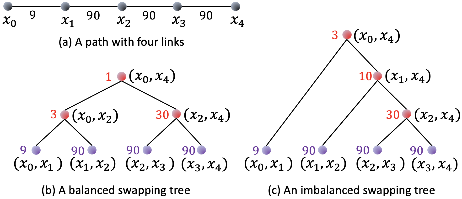
Figure 4: Consider the path in (a). The imbalanced tree of (b) has a higher EP generation rate than that of the balanced tree of (c). Here, the numbers represent the EP generation rates over adjacent links or node-pairs.

3.1 Problem Formulation

We now formulate the central problem of selecting multiple swapping trees for each given source-destination pair. Selection of multiple routes is a well-established strategy [32, 9, 27] to maximize entanglement rates.

Quantum Network Routing (QNR) Problem. Given a quantum network and a set of source-destination pairs $\{(s_{i},d_{i})\}$, the QNR problem is to determine a set $\mathcal{T}_{i}$ of swapping trees for each pair $(s_{i},d_{i})$ such that the sum of the EP rates of all the trees in $\bigcup_{i}\mathcal{T}_{i}$ is maximized under the following constraints:

• Node Constraints. For each node, the aggregate resources used by $\bigcup_{i}\mathcal{T}_{i}$ is less than the available resources; we formulate this formally below.

• Fidelity Constraints. Each swapping tree in $\bigcup_{i}\mathcal{T}_{i}$ satisfies the following: (a) Number of leaves is less than a given threshold $\tau_{l}$; this is to limit fidelity degradation due to gate operations. (b) Total memory storage time of any qubit is less than a given decoherence threshold $\tau_{d}$.

Informally, the swapping-trees may also satisfy some fairness constraint across the given source-destination pairs. A special case of the above QNR problem is to select a single tree for a source-destination pair; we address this in the next section.

Formulating Node Constraints. Consider a swapping tree $\mathcal{T}\in\bigcup_{i}\mathcal{T}_{i}$ over a path $P$. For each link $e\in P$, let $R(e,\mathcal{T})$ be the EP rate being used by $\mathcal{T}$ over the link $e$ in $P$. Let us define $R_{e}=\sum_{\mathcal{T}}R(e,\mathcal{T})$, and let $E(i)$ be the set of edges incident on $i$. Then, the node capacity constraint is formulated as follows.

$$1/\mbox{$t_{g}$} \geq \sum_{e\in E(i)}R_{e}/(\mbox{$p_{g}$}^{2}\mbox{$p_{e}$}^{2}\mbox{$p_{ob}$})\ \ \ \ \forall i\in V.$$ (2)

Also, the memory constraint is that for any node $i$, the memory available in $i$ should be more than $2x+y$ where $x$ is the number of swapping trees that use $i$ as an intermediate node and $y$ is the number of trees that use $i$ as an end node.

3.2 Related Works

There have been a few works in the recent years that have addressed generating long-distance EPs efficiently. All of these works have focused on selecting an efficient routing path for the swapping process ([8] also selects a path, but using a metric based on balanced trees). In addition, all except [8] have looked at the WaitLess protocol of generating the EPs. Recall that in the WaitLess model, selection of paths suffice, while in the Waiting model, one needs to consider selection of efficient swapping trees with high fidelity. Selection of optimal swapping trees is a fundamentally more challenging problem than selection of paths—and has not been addressed before, to the best of our knowledge. We start with discussing the WaitLess model works.

WaitLess Approaches. The most recent works to address the above problem are [32] and [9], both of which consider the WaitLess model. In particular, Shi and Qian [32] design a Dijkstra-like algorithm to construct an optimal path between a pair of nodes, when there are multiple links (channels) between adjacent nodes. Then, they use the algorithm iteratively to select multiple paths over multiple pairs of nodes. Chakraborty et al. [9] design a multi-commodity-flow like LP formulation to select routing paths for a set of source destination pairs. They map the operation-based fidelity constraint to the path length (as in [6]), and use node copies to model the constraint in the LP. However, they explicity assume that the link EP generation is deterministic—i.e., always succeeds. Among earlier relevant works, [27] proposes a greedy solution for grid networks, and [10] proposes virtual-path based routing in ring/grid networks.

Waiting Approach. Due to photon loss, establishing long-distance entanglement between remote nodes at $L$ distance by direct transmission yields EP rates that decay exponentially with $L$. DLCZ protocol [16, 30] broke this exponential barrier using $2^{k}$ equidistant intermediate nodes to perform entanglement-swapping operations, implicitly over a balanced binary tree, with a Waiting protocol; this makes the EP generation rate decay only polynomially in $L$. More recently, Caleffi [8] formulated the entanglement generation rate on a given path between two nodes, under the more realistic condition where the intermediate nodes in the path may not all be equidistant, but still considered only balanced trees. Their path-based metric was then used to select the optimal path by enumerating over the exponentially many paths in the network.

Our Approach (vs. [8]). Though [8] considers only balanced trees, its brute-force algorithm is literally impossible to run for networks more than a few tens of nodes (§7). In our work, we observe that a path has many swapping trees, and, in general, imbalanced trees may even be better; see Figure 4. Thus, we design a polynomial-time dynamic programming (DP) algorithm that delivers an optimal high-fidelity swapping-tree; our DP approach effectively considers all possible swapping trees, not just balanced ones (note that, even over a single path, there are exponentially many trees). Incorporation of fidelity (including decoherence) in our DP approach requires non-trivial observation and analysis (§4.2). Our Balanced-Tree Heuristic (§5) is closer to [8]’s work, in that both consider only balanced trees; however, we use heuristic metric that facilitates a polynomial-time Dijkstra-like heuristic to select the optimal path, while their recursive metric  (albeit more accurate than ours) is not amenable to an efficient (polynomial-time) search algorithm.

Other Works. In [21], Jiang et al. address a related problem; given a path with uniform link-lengths, they give an algorithm for selecting an optimal sequence of swapping and purification operations to produce an EP with fidelity constraints. In other recent works, Dahlberg et al [13] design physical and link layer protocols of a quantum network stack, and [23] proposes a data plane protocol to generate EPs within decoherence thresholds along a given routing path.

4 Optimal Algorithm for Single Tree

In this section, we consider a special case of the QNR problem, viz., the case wherein there is a single source-destination $(s,d)$ pair and the goal is to select a single swapping tree for the $(s,d)$ pair. For this special case, we design an optimal algorithm based on dynamic programming. This optimal algorithm can be used iteratively to develop an efficient heuristic for the general QNR problem, as in §6.

QNR-SP Problem. Given a quantum network and a source-destination pair $(s,d)$, the QNR-SP problem is to determine a single swapping tree that maximizes the expected generation rate (i.e., minimizes the expected generation latency) of EPs over $(s,d)$, under the capacity and fidelity constraints.

For homogeneous nodes and link parameters, it is easy to see that the best swapping-tree is the balanced or almost-balanced tree over the shortest path. We note that QNR-SP is not a special case of QNR in the formal sense; e.g., the LP algorithm (§A) for QNR cannot be used for the QNR-SP problem, due to the single tree requirement (LP may produce multiple trees). As described in §3.2, the QNR-SP problem has been addressed before in  [32, 8] under different models.

4.1 Dynamic Programming (DP) Formulation

First, we note that a Dijkstra-like shortest path approach which builds a shortest-path tree greedily doesn’t work for the QNR-SP problem—mainly, because the task is to find an optimal tree rather than an optimal path. As noted before, a routing path can have exponentially many swapping trees over it, with different generation latency. The recursive expression for computing the generation latency given in §3 suggests that a dynamic programming (DP) approach, similar to the Bellman-Ford or Floyd-Warshall’s classical algorithms for shortest paths, may be applicable for the QNR-SP problem. However, we need to “combine” trees rather than paths in the recursive step of a DP approach. Consequently, we were unable to design a DP approach based on the Floyd-Warshall’s approach, but, are able to extend the Bellman-Ford approach for the QNR-SP problem after addressing a few challenges discussed below.

DP Formulation. We start with designing a DP algorithm without worrying about the decoherence constraint; we incorporate the decoherence constraint in the next subsection. Given a network, let $T[i,j,h]$ be the optimal expected latency of generating EP pairs over $(i,j)$ using a swapping tree of height at most $h$. Note that $T[i,j,0]$ for adjacent nodes $(i,j)$ can be given by $\frac{\mbox{$t_{g}$}}{\mbox{$p_{g}$}^{2}\mbox{$p_{e}$}^{2}\mbox{$p_{ob}$}}$. Now, based on Eqn 1, we start with the following equation for computing $T[i,j,h]$ in terms of smaller-height swapping trees.

$$T[i,j,h] = \min(T[i,j,h-1],(\frac{3}{2}B+\mbox{$t_{c}$}+\mbox{$t_{b}$})/\mbox{$p_{b}$}),{\rm where}$$ (3)

$$B = \min_{k\in V}\ \ \max(T[i,k,h-1],T[k,j,h-1])$$

However, there are three issues that need to be addressed before the above formulation can be turned into a viable algorithm. We address these in the below three paragraphs.

(1) The 3/2 Factor; Throttled Trees. As mentioned in §3, the 3/2 factor is an accurate estimate if the corresponding $T$’s are equal. However, in the above equation, $T[i,k,h-1]$ and $T[k,j,h-1]$ may not be equal. In our overall methodology, to conserve node and link resources, we post-process or "throttle" the swapping-tree obtained from the DP algorithm by increasing the generation latencies of some of the non-root nodes such that (i) the latencies of siblings are equalized, and (ii) the parents latency is related to the children’s latency by Eqn. 1. We refer to this post-processing at throttling, and a tree that satisfies the above conditions as a throttled tree. Note that throttling does not alter the generation latency of the root and thus the overall tree; we prove the optimality of the overall algorithm formally in Theorem 2). Below, we motivate throttling, and describe how it is achieved.

Justification. In a given swapping tree, consider a pair of siblings $x$ and $y$ that have unequal generation latencies/rates. Let $x$ be the one with a lower latency (higher rate). Then, $x$ will likely have to discard many EPs while waiting for an EP from $y$. To minimize this discarding of EPs from $x$ and to conserve underlying network resources so that they can be used in other swapping trees (in a general QNR solution), we “throttle”, increase (decrease) the generation latency (rate) of, the sibling $x$ to match that of $y$.

Throttling Process. Consider a pair of siblings $x$ and $y$ in the tree; let their parent be $z$. Let $T_{x},T_{y},$ and $T_{z}$ be their current generation latencies, such that $T_{z}=(\frac{3}{2}\max(T_{x},T_{y})+\mbox{$t_{c}$}+\mbox{$t_{b}$})/\mbox{$p_{b}$}$. There are two potential steps: (i) If the parent’s latency is to be kept unchanged, but $T_{x}<T_{y}$ then $T_{x}$ is increased to $T_{y}$ and thus, makes the above equation valid. (ii) If the parents latency $T_{z}$ is increased to $T$ (due to the first step, with $z$ as a sibling), then we increase the latencies of both $x$ and $y$ $2/3(T\mbox{$p_{b}$}-\mbox{$t_{c}$}-\mbox{$t_{b}$})$. It is easy to see that applying the two steps iteratively from the root’s children yields a throttled tree, as defined above.

(2) Capacity Violation at Node $k$. Note that the middle/common node $k$ in Eqn. 3 may violate (node) capacity constraints in the merged tree corresponding to $T[i,k,h]$, as it may use its full capacity in the trees corresponding to $T[i,k,h-1]$ and $T[k,j,h-1]$. We address the above by adding two additional parameters to the sub-problems $T[]$, corresponding to “usage percentage” of the end nodes. In particular, we define $T[i,j,h,u_{i},u_{j}]$ as the optimal latency of a swapping tree of height at most $h$, under the constraint that the end nodes $i$ and $j$ use at most $u_{i}$ and $u_{j}$ percentage of the respective node generation capacities; here, $u_{i}$ and $u_{j}$ can be positive integers between 1 and 100. The base case $T[i,j,0,u_{i},u_{j}]$ for adjacent nodes $(i,j)$ is given by $\frac{\mbox{$t_{g}$}\min(u_{i},u_{j})}{\mbox{$p_{g}$}^{2}\mbox{$p_{e}$}^{2}\mbox{$p_{ob}$}}$. Eqn. 3 is modified as follows to accommodate the additional usage parameters.

$$T[i,j,h,u_{i},u_{j}]=\min(T[i,j,h-1,u_{i},u_{j}],(\frac{3}{2}B+\mbox{$t_{c}$}+\mbox{$t_{b}$})/\mbox{$p_{b}$}),$$ (4)

$${\rm where}\ B=\min_{k,\ u+u^{\prime}=100}\max(T[i,k,h-1,u_{i},u],T[k,j,h-1,u^{\prime},u_{j}])$$

(3) Ensuring Disjoint Subtrees. Note that Eqn. 3 implicitly assumes that the swapping trees corresponding to the latency values $T[i,k,h-1]$ and $T[k,j,h-1]$ are over disjoint paths, i.e., there is no node $v$ such that both the paths contain $v$. If there is a common node $v$, then the combined tree corresponding to $[i,j,h]$ may violate the node capacity constraints at $v$. This issue also arises in the classical Bellman Ford’s or Floyd-Warshall’s algorithms for shortest weighted paths, but is harmless with the assumption of positive-weighted cycles. We resolve the issue similarly here via the below lemma (see Appendix C for the proof).

Lemma 1

Consider two swapping trees $\mathcal{T}_{ik}$ and $\mathcal{T}_{kj}$ each of height at most $h-1$ over paths $P_{1}:i\leadsto v\leadsto k$ and $P_{2}:k\leadsto v\leadsto j$, each of which contains a common node $v\not=k$. Then there exists two swapping trees $\mathcal{T}_{iv}$ and $\mathcal{T}_{vj}$ each of height at most $h-1$ over paths $P^{\prime}_{1}:i\leadsto v$ and $P^{\prime}_{2}:v\leadsto j$ such that: (i) $P^{\prime}_{1}$ is a subset of $P_{1}$, and $P^{\prime}_{2}$ is a subset of $P_{2}$, and (ii) generation latency of $\mathcal{T}_{iv}$ is no greater than that of $\mathcal{T}_{ik}$, and generation latency of $\mathcal{T}_{vj}$ is no greater than that of $\mathcal{T}_{kj}$.  

Lemma 1 implies that if the swapping trees $\mathcal{T}_{ik}$ and $\mathcal{T}_{kj}$ corresponding to the latency values $T[i,k,h-1]$ and $T[k,j,h-1]$ have a common node, then there exist swapping trees that have matching or better latency without common nodes that can be used to build an optimal-latency tree over $(i,j)$.

Overall DP Algorithm and Optimality. Our DP-based algorithm for the QNR-SP problem for a given $(s,d)$ pair is as follows. We use a DP formulation based on Eqn. 4 and the corresponding base case values to compute optimal generation latency $T[s,d,h,100,100]$ and the corresponding swapping tree $\mathcal{T}$. Then, we throttle the tree $\mathcal{T}$ as described in paragraph (1) above. The below theorem states that the throttled tree thus obtained has the optimal (minimum) expected generation latency among all throttled trees.

Theorem 2

The above described DP-based algorithm returns a throttled swapping tree over $(s,d)$ with minimum expected generation latency (maximum expected generation rate) among all throttled trees over the given $(s,d)$ pair.  

4.2 Incorporating Fidelity Constraints

Till now, we have ignored the fidelity constraints. We incorporate them in this section, by extending our DP formulation from the previous section. Limiting the decoherence, i.e., the qubit storage time, is challenging and is addressed first below. Limiting the number of leaves of a swapping tree is relatively easier, and is discussed next. We start with a definition.

Definition 1

(Qubit/Tree Age.) Given a swapping tree, the total time spent by a qubit in a swapping tree is the time spent from its “birth” via an atom-photon EP generation at a node till its consumption in a swapping operation or in generation of the tree’s root EP. We refer to this as a qubit’s age. The maximum age over all qubits in a swapping tree is called the tree’s (expected) age.

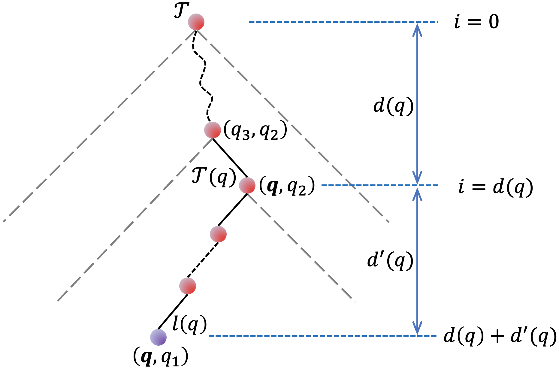
Figure 5: Qubit parameters in a swapping tree used to compute the age of a qubit $q$ at a leaf node $l(q)$. Here, $l(q)$ is the left-most leaf of the subtree $\mathcal{T}(q)$.

Estimating Qubit Age in a Swapping Tree. Consider a throttled swapping tree $\mathcal{T}$, with a generation latency of $T$. Consider two siblings $(A,B)$ and $(B,C)$ at a depth of $i$ ($i>0$) from $\mathcal{T}$’s root. If we ignore the $t_{c}$ and $t_{b}$ terms in Eqn. 1, then the expected generation latency $T(i)$ of both $(A,B)$ and $(B,C)$ being at depth $i$ is given by: $T(i)=\frac{T}{2}(\frac{2}{3}\mbox{$p_{b}$})^{i}.$ Also, note that only one of the EPs $(A,B)$ or $(B,C)$ waits for $T(i)$ time on an average. Thus, the expected waiting times for each of the four qubits is $T(i)/2$.

Based on the above, we can now easily estimate the total waiting by a qubit $q$ (referred to as $q$’s age) before it is destroyed in a swapping operation. Let $l(q)$ be the leaf, i.e. the link EP, of $\mathcal{T}$ that contains the qubit $q$. Let $\mathcal{T}(q)$ be the maximal subtree in $\mathcal{T}$ such that $l(q)$ is either its right-most or left-most leaf. Note that $\mathcal{T}(q)$ is well defined for a tree $\mathcal{T}$ and a qubit $q$. Let $d(q)$ be the depth of the root of $\mathcal{T}(q)$ in $\mathcal{T}$, and let $d^{\prime}(q)$ be the depth of $l(q)$ in the subtree $\mathcal{T}(q)$. See Fig. 5. The expected age $A(q)$ of $q$ can be estimated as follows. Note that age of $q$ is the total waiting by $q$ at each of $l(q)$’s ancestors in $\mathcal{T}(q)$; also note that at $\mathcal{T}(q)$’s root, the qubit $q$ is destroyed, and hence, $q$ does not age at any ancestor of $T(q)$’s root. It is easy to see that the expected age $A(q)$ is:

$$A(q)=\left(\sum_{i=d(q)}^{d(q)+d^{\prime}(q)}T(i)/2\right)+(t_{ob}+t_{p})$$

Above, the last term is the time spent by $q$ waiting for its link EP to be established and is given by sum of optical-BSM ($t_{ob}$) and photon transmission latency ($t_{p}$). Note that the actual age of a qubit $q$ is some distribution with the above mean. We observe the following.

Observation 2

Given a swapping tree $\mathcal{T}$, let $\mathcal{T}_{l}$ and $\mathcal{T}_{r}$ be its left and right children. If the atomic BSM probability $p_{b}$ is $\leq$ 75%, then the expected age of the right-most or left-most descendant of either $\mathcal{T}_{l}$ or $\mathcal{T}_{r}$ is greater than the expected age of any other qubit in the tree.

DP Formulation with Decoherence/Age Constraint. If we assume the atomic BSM probability $p_{b}$ $\leq$ 75%, then we can design a DP algorithm for the QNR-SP problem with the decoherence constraint, as follows. Let $T[i,j,h,h_{ll},h_{lr},h_{rl},h_{rr},u_{i},u_{j}]$ be the optimal latency from a swapping tree of height at most $h$, whose root’s left (right) child’s left-most and right-most descendants are at depths of (exactly) $h_{ll}$ and $h_{lr}$ ($h_{rl}$ and $h_{rr}$), each of which is upper bounded by $h$. Here, $u_{i}$ and $u_{j}$ parameters are as before. Note that $T[i,j,1,0,0,0,0,u_{i},u_{j}]=\frac{\mbox{$t_{g}$}\min(u_{i},u_{j})}{\mbox{$p_{g}$}^{2}\mbox{$p_{e}$}^{2}\mbox{$p_{ob}$}}.$ We have:

$$T[i,j,h,h_{ll},h_{lr},h_{rl},h_{rr},u_{i},u_{j}]=\min((\frac{3}{2}B+\mbox{$t_{c}$}+\mbox{$t_{b}$})/\mbox{$p_{b}$}),\ \$$ (5)

$$B=\min_{k,\ g_{i}^{\prime}s,\ u+u^{\prime}=100}\max(T[i,k,h-1,h_{ll}-1,g_{1},g_{2},h_{lr}-1,u_{i},u],$$

$$\hskip 72.26999ptT[k,j,h-1,h_{rl}-1,g_{3},g_{4},h_{rr}-1,u^{\prime},u_{j}])$$

The above formulation will give us the optimal latency swapping-tree for each combination of $(h_{ll},h_{lr},h_{rl},h_{rr})$. We remove the trees that violate the decoherence constraint, and pick the minimum-latency tree from the remaining. This gives us a swapping tree with optimal latency under the decoherence constraint. The proof of optimality easily follows.

Constraint on Number of Leaves. Limiting the number of leaves to $\tau_{l}$ can be easily done by adding another parameter for number of leaves in the $T[]$ array/function above. This adds another factor of $O(n^{2})$ to the time complexity, as we need to check for all combination of number of leaves in the two subtrees. To optimize, we can now replace the height parameter, but keeping the height parameters aids in parallelism, as described below.

Time Complexity; DP-OPT and DP-Approx Algorithms Note that, in Eqn. 5 above, we can pre-compute $\min_{g_{1},g_{2}}$ $T[\ldots,g_{1},g_{2},\ldots]$ and similarly $\min_{g_{3},g_{4}}T[\ldots,g_{3},g_{4},\ldots]$ before computing $B$. With this, the time complexity of the DP formulation becomes $O(n^{9})$, which can be further reduced $O(n^{5}(\log n)^{4})$ if we assume height of a tree to be at most $(c\log n)$ for some constant $c$. For a real-time routing application, the above time complexity is still high—as the algorithm can take a few minutes on a single core. However, as the algorithm lends to obvious parallelism, it can be executed in as little as $O((\log n)^{2})$ time with sufficiently many cores, using the height parameter sequentially. We can also reduce the sequential time complexity to $O(n^{5})$, by approximating the maximum qubit’s age in a tree to the generation latency of the tree, which is a at most $3/(2\mbox{$p_{b}$})$ the actual value. Note that maximum age of a qubit is at least $2T\mbox{$p_{b}$}/3$ and at most $T$, where $T$ is the generation latency of the tree. Finally, we can make the algorithm more efficient by assuming the usage parameter values to be 50%. We refer to the $O(n^{5})$ algorithm with the above assumptions as DP-Approx, and the $O(n^{5}(\log n)^{4})$ algorithm based on Eqn. 5 as DP-OPT. Both algorithms use throttling after the DP formulation.

5 Balanced-Tree Heuristic for QNR-SP

The DP-based algorithms presented in §4 for the QNR-SP problem have high time complexity, and thus, may not be practical for real-time route finding in large networks. In this section, we develop an almost-linear time heuristic for the QNR-SP problem, based on the classic Dijkstra shortest path algorithm; the designed heuristic performs close to the DP-based algorithms in our empirical studies.

Basic Idea. The main reason for the high-complexity of our DP-based algorithms in §4 is that the goal of the QNR-SP problem is to select an optimal swapping tree rather than a path. One way to circumvent this challenge efficiently while still select a near-optimal swapping tree, is to restrict ourselves to only "balanced" swapping trees. This restriction allows us to think in terms of selection of paths—rather than trees—since each path has a unique balanced swapping tree. We can then develop an appropriate path metric based on above, and design a Dijkstra-like algorithm to select an $(s,d)$ path that has the optimal metric value. We note that Caleffi [8] also proposed a path metric based on balanced swapping trees, but their metric, though accurate, only had a recursive formulation without a closed-form expression—and hence, was ultimately not useful in designing an efficient algorithm. In contrast, we develop an approximate metric with a closed-form expression, based on the "bottleneck" link, as follows.

Path Metric $M$. Consider a path $P=(s,x_{1},x_{2},\ldots,x_{n},d)$ from $s$ to $d$, with links $(s,x1),(x1,x2),\ldots,(x_{n},d)$ with given EP latencies. We define the path metric for path $P$, $M(P)$, as the EP generation latency of a balanced swapping over $P$, which can be estimated as follows. Let $L$ be the link in $P$ with maximum generation latency. If $L$’s depth (distance from the root) is the maximum in a throttled swapping tree, then we can easily determine the accurate generation latency of the tree. However, in general, $L$ may not have the maximum depth, in which case we can still estimate the tree’s latency approximately, if the tree is balanced, as follows. In balanced swapping trees, assuming the maximum latency link $L$ to be at the maximum depth, gives us a constant-factor approximation of the tree’s generation latency. Thus, let us assume $L$ to be at the maximum depth of a balanced tree over $P$; this maximum depth is $d=\lceil(\log_{2}|P|)\rceil$. Let the generation latency of $L$ be $T_{L}$. If we ignore the $\mbox{$t_{b}$}+\mbox{$t_{c}$}$ term in Eqn. 1, then, the generation latency of a throttled swapping tree can be easily estimated to $T(\frac{3}{2\mbox{$p_{b}$}})^{d}.$ The term $\mbox{$t_{b}$}+\mbox{$t_{c}$}$ can also be incorporated as follows. Let $T(i)$ denote the expected latency of the ancestor of $L$ at a distance $i$ from $L$. Then, we get the recursive equation: $T(i)=(\frac{3}{2}T(i-1)+\mbox{$t_{b}$}+\mbox{$t_{c}$})/\mbox{$p_{b}$}.$ Then, the path metric value $M(P)$ for path $P$ is given by $T(d)$, the generation latency of the tree’s root at a distance of $d$ from $L$, and is equal to:

$$M(P)=T(d)=\bar{p}^{d}T_{L}+[(\bar{p}-1)/(\bar{p}^{d}-1)](\mbox{$t_{b}$}+\mbox{$t_{c}$})/\mbox{$p_{b}$}$$

where $\bar{p}=3/(2\mbox{$p_{b}$})$ and $d=\lceil(\log_{2}|P|)\rceil$. The above is a (1+3/(2$p_{b}$))-factor approximation latency of a balanced and throttled swapping tree over $P$; this can be shown easily using analysis from §4.2.

Optimal Balanced-Tree Selection. The above path-metric $M()$ is a monotonically increasing function over paths, i.e., if a path $P_{1}$ is a sub-sequence of another path $P_{2}$, then $M(P_{1})\leq M(P_{2})$. Thus, we can tailor the classical Dijkstra’s shortest path algorithm to select a $(s,d)$ path with minimum $M(P)$ value, using the link’s EP generation latencies as their weights. We refer to this algorithm as Balanced-Tree, and it can be implemented with a time complexity of $O(m+n\log n)$ using Fibonacci heaps, where $m$ is the number of edges and $n$ is the number nodes in the network.

Incorporating Fidelity Constraints. Fidelity constraints in our path-metric based setting can be handled by essentially computing the optimal path for each path-length (number of hops in the path) up to $\tau_{l}$, and then pick the best path among them that satisfies the fidelity constraints. The obviously limits the number of leaves to $\tau_{l}$ and addresses the operations-based fidelity degradation. The above also address the decoherence/age constraint, since it is easy to see (from analysis in §4.2) that a age of a balanced swapping tree can be very closely approximated in terms of the latency and the number of leaves. Now, to compute the optimal path for each path-length, we can use a simple dynamic programming approach that run in $O(m\tau_{l})$ time where $m$ is the number of edges and $\tau_{l}$ is the constraint on number of leaves.

6 ITER: Iterative QNR Heuristic

The general QNR problem can be forumulated in terms of hypergraph flows and solved using LP (see Appendix A). Although polynomial-time and provably optimal, the LP-based approach has a very high time-complexity for it to be practically useful. Here, we develop an efficient heuristic for the QNR problem by iteratively using an QNR-SP algorithm.

ITER Heuristic. To solve the QNR problem efficiently, we apply the efficient DP-Approx algorithm iteratively—finding an efficient swapping tree in each iteration for one of the $(s_{i},d_{i})$ pairs. The proposed algorithm is similar to the classical Ford-Fulkerson augmenting path algorithm for the max network flow problem at a high level, with some low level and theoretical differences as discussed below. The iterative-DP-Approx algorithm for the QNR problem consists of the following steps:

• Given a network, we compute maximum EP generation rates for each network link using Eqn. 6. Use these as weights on the link.

• For each $(s_{i},d_{i})$ pair, use DP-Approx algorithm to find the optimal path $P_{i}$, under the capacity and fidelity constraints. Consider a throttled and balanced swapping tree $\mathcal{T}_{i}$ over $P_{i}$. Let $\mathcal{T}^{*}$ be the swapping tree with highest generation rate; if this rate is below a certain threshold, then quit.

• Construct a residual network graph by subtracting the resources used by $\mathcal{T}^{*}$, using Eqns. 7.

• Go to step (1).

Before we present the expressions required above, we would like to point out key differences of our context with the classic network flow setting. Even though we are augmenting our solution one path at a time, the network resources are fundamentally being used by swapping trees created over these paths. These path-flows don’t really have a direction of flow, but we can assign them a symbolic direction from source to the direction. Even with these symbolic directions, the flows in opposite directions over any edge $k$ do not "cancel" each other as in the classical network flow. Moreover, flow conservation law doesn’t hold in our context (e.g., even a path may not use same link rates on all links, due to them being at different depths of the tree), and thus, the max-flow min-cut theorem doesn’t hold. Thus, ITER may not give an optimal solution, even for a single $(s,d)$ pair.

Link EP Generation Rate/Latency. Consider a pair of network node $i$ and $j$ with corresponding current (residual) values of node latencies as $\mbox{$t_{g}$}(i)$ and $\mbox{$t_{g}$}(j)$. Assuming $p_{g}$ values to be same for both nodes, the minimum EP link rate for $(i,j)$ is then given by

$$\min(1/\mbox{$t_{g}$}(i),1/\mbox{$t_{g}$}(j))\mbox{$p_{g}$}^{2}\mbox{$p_{e}$}^{2}\mbox{$p_{ob}$}.$$ (6)

Residual Node Capacities. Let $P$ be a path added by ITER, at some earlier stage, and let $\mathcal{T}$ be the corresponding throttled swapping tree over $P$. As in §3, let $R(e,\mathcal{T})$ be the EP generation rate being used by $\mathcal{T}$ over a link $e\in P$, $R_{e}=\sum_{\mathcal{T}}R(e,\mathcal{T})$, and $E(i)$ be the edges incident on $i$. Then, the residual node rates can be calculated similar to Eqn. 2 as follows. Below, $\mbox{$t_{g}$}^{\prime}(i)$ is the original value.

$$1/\mbox{$t_{g}$}(i)=1/\mbox{$t_{g}$}^{\prime}(i)-\sum_{e\in E(i)}R_{e}/(\mbox{$p_{g}$}^{2}\mbox{$p_{e}$}^{2}\mbox{$p_{ob}$})\ \ \ \ \forall i\in V.$$ (7)

The residual memory capacity is easy to compute—each path/tree uses 2 memory units for each intermediate node, and 1 memory unit for the end nodes.

7 Evaluations

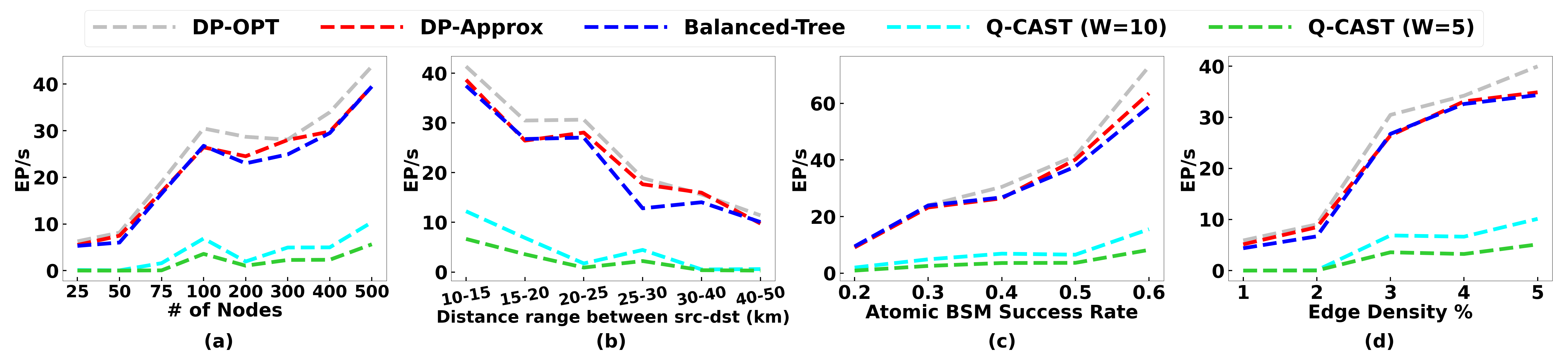
Figure 6: QNR-SP Problem: EP Generation Rates for varying parameters.

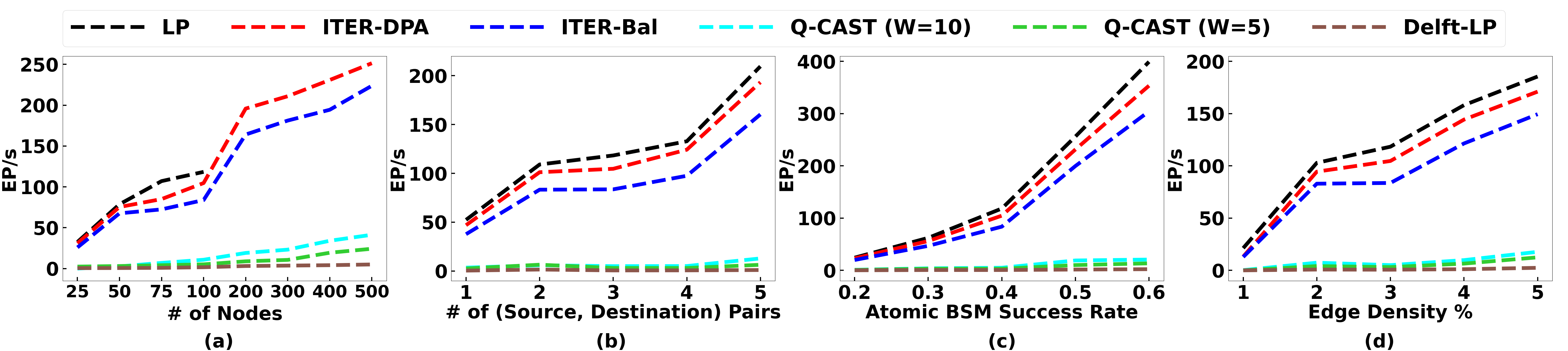
Figure 7: QNR Problem: EP Generation Rates for varying parameters.

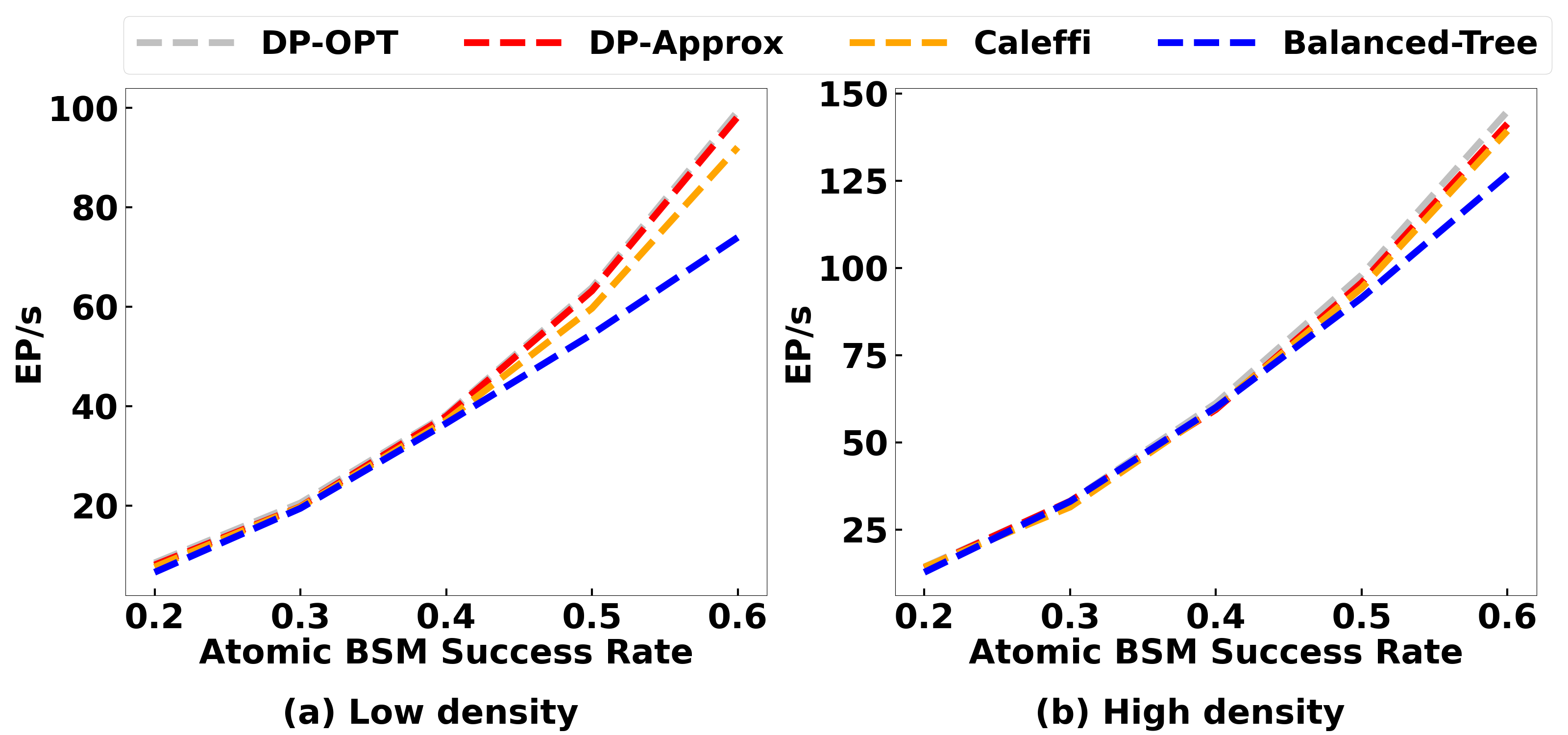
Figure 8: Compare the performance with Caleffi in a (a) low density network and a (b) high density network.

The goal of our evaluations is to compare the EP generation rates, evaluate the fidelity of generated EPs, and validate our analytical models. We implement the various schemes over a discrete event simulator for QNs called NetSquid [12]. The NetSquid simulator accurately models various QN components/aspects, and in particular, we are able to define various QN components and simulate swapping-trees protocols by by implementing gate operations in entanglement swapping.

Swapping Tree Protocol. Our algorithms compute swapping tree(s), and we need a way to implement them on a network. We build our protocol on top of the link-layer of [13], which is delegated with the task of continuously generating EPs on a link at a desired rate (as per the swapping tree specifications). Note that a link $(a,b)$ may be in multiple swapping trees, and hence, may need to handle multiple link-layer requests at the same time; we implement such link-layer requests by creating independent atom-photon generators at $a$ and $b$, with one pair of synchronized generators for each link-layer request. As the links generate continuous EPs at desired rates, we need a protocol to swap the EPs. Omitting the tedious bookkeeping details, the key aspect of the protocol is that swap operation is done only when both the appropriate EP pairs have arrived. We implement all the gate operations (including, atomic and optical BSMs) within NetSquid to keep track of the fidelity of the qubits. On BSM success, the swapping node transmits classical bits to the end node which manipulates its qubit, and send the final ack to the other end node. On BSM failure, a classical ack is send to all descendant link leaves, so that they can now start accepting new link EPs; note that in our protocol, a link $l$ does not accept any more EPs, while its ancestor is waiting for its sibling’s EP.

Simulation Setting. We use a similar setting as in the recent work [32]. By default, we use a network spread over an area of $100km\times 100km$. We use the Waxman model [38], used to create Internet topologies, to randomly distribute the nodes and create links; we use the maximum link distance to be 10km. We vary the number of nodes from 25 to 500, with 100 as the default value. We choose the two parameters in the Waxman model to maintain the number of links to 3% of the complete graph (to ensure an average degree of 3 to 15 nodes). For the QNR-SP problem, we pick $(s,d)$ pairs within a certain range of distance, with the default being 15-20 kms; for the QNR problem, we extend this range to 10-30 kms.

Parameter Values. We use parameter values as the ones used in [8], and vary some of them. In particular, we use atomic-BSM probability of success ($p_{b}$) to be 0.4 and latency ($t_{b}$) to be 10 $\mu$ secs; in some plots, we vary $p_{b}$ from 0.2 to 0.6. The optimal-BSM probability of success ($p_{ob}$) is half of $p_{b}$. We use atom-photon generation times ($t_{g}$) and probability of success ($p_{g}$) as 50 $\mu$sec and 0.33 respectively. Finally, we use photon transmission success probability as $e^{-d/(2L)}$ [8] where $L$ is the channel attenuation length (chosen as 20km for an optical fiber) and $d$ is the distance between the nodes. Each node’s memory size is randomly chosen within a range of 15 to 20 units. Fidelity is modeled in NetSquid using two parameter values, viz., depolarization (for decoherence) and dephasing (for operations-driven) rates. We conservatively choose a depolarization rate of 0.01 such that the fidelity after 1 min is 90%, based on demonstrated coherence times of several minutes [34, 29] to hours [40, 37]. Similarly, we choose a dephasing rate of 1000 which corresponds to a link EP fidelity of 99.5% [9]. In our schemes, we conservatively discard qubits/EPs that age more than a second.

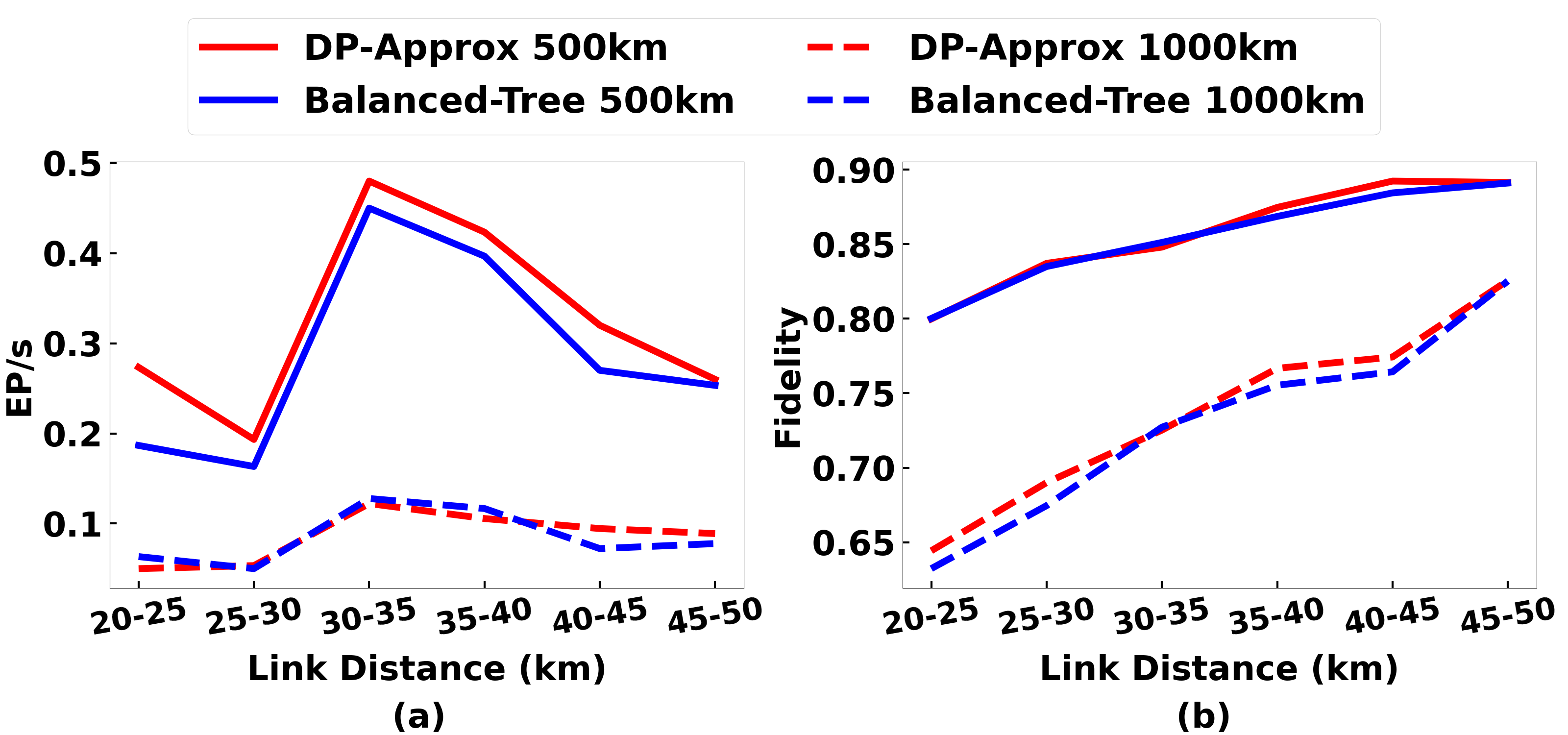
Figure 9: (a) EP Rates, and (b) Fidelity, over linear paths.

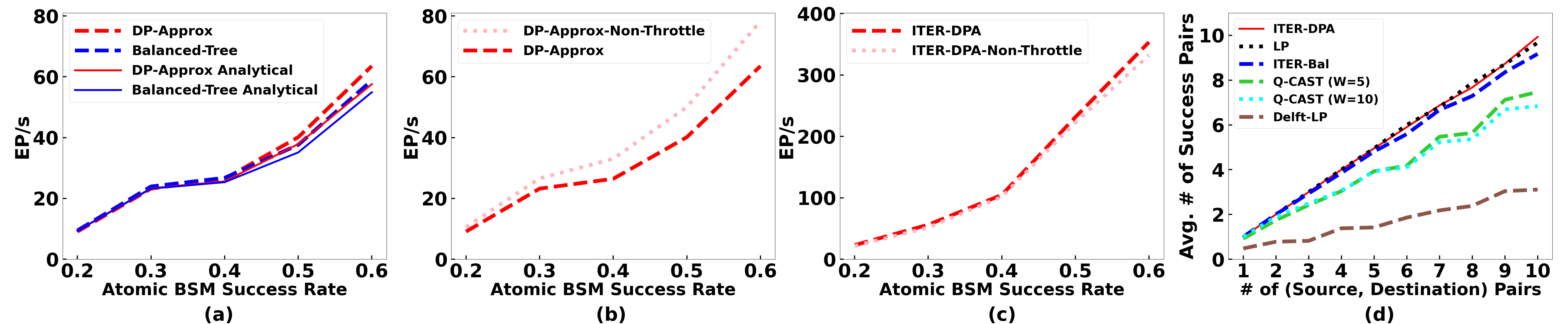
Figure 10: Comparing with Analytical Results. (a) Analytical vs. Simulation Results. (b) Throttled vs. Non-Throttled Trees (QNR-SP). (c) Throttled vs. Non-Throttled Trees (QNR). (d) Fairness Measure.

Algorithms and Performance Metrics. To compare our techniques with prior approaches, we implement most recently proposed approaches, viz., Q-Cast approach from [32] and the LP approach from [9] which we refer to as Delft-LP.  [8] proposes an exponential-time approach, and is thus compared only for small networks. The [27] and [10] approaches are not compared as they were found to be inferior to Q-Cast in [32]. For all algorithm except for Q-Cast, we use only one link between adjacent nodes, since only Q-Cast takes advantage of multiple links in a creative way. In particular, for Q-Cast, we use $W=1,5$, or 10 sub-links ([32] calls them channels) on each link, with the node and link "capacity" divided equally among the them. Note that each node requires $2W$ memories, 2 for each sub-link. The Delft-LP approach explicitly assume the generation of link EPs is deterministic, i.e., the value $\mbox{$p_{g}$}^{2}\mbox{$p_{e}$}^{2}\mbox{$p_{ob}$}$ is 1, and do not model node generation rates. We address these differences by extending their LP formulation: (i) We add a constraint on node generation rates, and (ii) add a $\mbox{$p_{g}$}^{2}\mbox{$p_{e}$}(i,j)^{2}\mbox{$p_{ob}$}$ factor to each link $(i,j)$ in any path extracted from their LP solution. Among our schemes, we use DP-OPT, DP-Approx and Balanced-Tree (see §4.2) for the QNR-SP problem, and LP (Appendix A) and ITER schemes for the QNR problem. For ITER, we use two schemes: ITER-DPA and ITER-Bal, which iterate over DP-Approx and Balanced-Tree respectively. We compare the schemes largely in terms of EP generation rates; we also compare the execution times and EPs fidelity.

Comparison with [8] for QNR-SP Problem. Note that [8] gives only an QNR-SP algorithm referred to as Caleffi; it takes exponential-time making it infeasible to run for network sizes much larger than 15-20. In particular, for network sizes 17-20, it takes several hours, and our preliminary analysis suggests that it will take of the order of $10^{40}$ years on our 100-node network. See Appendix D. Thus, we use a small network of 15 nodes over a 25km $\times$ 25km area; we consider average node degrees of 3 or 6. See Fig.8. We see that DP-OPT outperforms Caleffi by 10% on a average for the sparser graph and minimally for the denser graph. However, for some instances, DP-OPT outperformed Caleffi by as much as 300% (see Appendix E). We see that DP-Approx performs similar to DP-OPT, while Balanced-Tree is outperformed slightly by Caleffi; however, for this small network, since the DP-OPT and DP-Approx algorithms only take 10-100s of msecs (Appendix D), Balanced-Tree need not be used in practice.

QNR-SP Problem (Single Tree) Results. We start with comparing various schemes for the QNR-SP problem, in terms of EP generation rate. We compare DP-Approx, DP-OPT, Balanced-Tree, and Q-Cast; note that the LP schemes can’t be used to select a single tree, as they turn into ILPs. See Fig. 6, where we plot the EP generation rate for various schemes for varying number of nodes, $(s,d)$ distance, $p_{b}$, and network link density. We observe that DP-Approx and DP-OPT perform very closely, with the Balanced-Tree heuristic performing close to them; all these three schemes outperform the Q-Cast schemes (for $W=5,10$ sub-links) by an order of magnitude. We don’t plot Q-Cast for $W=1$ sub-links, as it performs much worse (less than $10^{-3}$ EP/sec). We note that Q-Cast’s EP rates here are much lower than the ones published in [32], because [32] uses link EP success probability of 0.1 or more, while in our more realistic model, the link EP success probability is $\mbox{$p_{g}$}^{2}\mbox{$p_{e}$}^{2}\mbox{$p_{ob}$}=0.012$ for the default $p_{b}$ value. We reiterate that our schemes require only 2 memory units per node, while the Q-Cast schemes requires $2W$ units. The main reason for poor performance of Q-Cast (in spite of higher memory and link synchronization) is that, in the WaitLess model, the EP generation over a path is a very low probability event—essentially $p^{l}$ where $p$ is the link-EP success probability and $l$ is the path length, for the case of $W=1$ (the analysis for higher $W$’s is involved [32]). In addition, we see that performance increases with increase in $p_{b}$, number of nodes, or network link density, as expected due to availability of better trees/paths; it also increases with decrease in $(s,d)$ distance as fewer hops are needed.

QNR Problem Results. We now present performance comparison of various schemes for the QNR problem. Here, we compare the following schemes: ITER-DPA, ITER-Bal, Delft-LP, and Q-Cast with the optimal LP as the benchmark for comparison (LP wasn’t feasible to run for more than 100 nodes). See Fig. 7. Our observations are similar to that for the QNR-SP problem results. We see that in all plots, LP being optimal performs the best, but is closely matched by ITER-DPA and the efficient heuristic ITER-Bal. Our schemes outperform both Delft-LP and Q-Cast by an order of magnitude, for the same reason as mentioned above.

Fidelity and Long-Distance Entanglements. We now investigate the fidelity of the EPs generated. First, we note that the Q-Cast and Delft-LP schemes will incur near-zero decoherence as they involve only transient storage. Decoherence for other schemes is also negligible as the EP generation latencies (10s of msecs) is much less than the coherence time. The operations-driven fidelity loss is expected to be similar for all schemes, as they all roughly use the same order of links. Overall, we observed fidelities of 94-97% across all schemes (not shown), with our schemes also performing better sometimes due to smaller number of leaves.

To test the limits of the schemes in terms of decoherence and fidelity, we consider a long path network and estimate fidelity of EPs generated by schemes for increasing distances and link-lengths (link success probability decreases with increasing link length). Fig. 9(a)-(b) shows EP generation rates and fidelity for path lengths of 500km and 1000km for varying link lengths, for the single-tree schemes DP-Approx and Balanced-Tree. Q-Cast and Delft-LP are not shown as their EP rate is near-zero ($\leq 10^{-20}$) at these distances. We observe that our schemes yield EPs with qubit fidelities of 80-90% and 65-83% for 500km and 1000km paths respectively, with EP rates of 0.05 to 0.5/sec. These are viable results—since qubit copies with fidelities higher than 50% can be purified to smaller copies with arbitrarily higher fidelities [4, 5].

Validating the Analysis; Fairness. Fig. 10(a) compares the EP generation rates as measured by the analytical formulae and the actual simulations for the QNR-SP algorithms DP-Approx and Balanced-Tree. We observe that they match closely, validating our assumption of 3/2 factor in Eqn. 1 and of exponential distributions at higher levels of the tree, and of the path metric $M()$ for Balanced-Tree. Fig. 10(b)-(c) plots the EP generation rates for throttled and non-throttled trees. We see that the throttled tree underperforms the non-throttled tree by only a small margin for the single-tree case; however, for the multi-tree ITER-Bal algorithm, the throttled trees perform better as they are able to use the resources efficiently. Fig. 10(d) plots the average number of $(s,d)$ pairs that get at least one tree/path for varying number of requests; we see that our schemes exhibit 90-99% fairness.

Execution Times. We ran our simulations on an Intel i7-8700 CPU machine, and observed that the WaitLess algorithms as well our Balanced-Tree and ITER-Bal heuristics run in fraction of a second even for a 500-node network; thus, they can be used in real-time. Note that since our problems depend on real-time network state (residual capacities), the algorithms must run very fast. The other algorithms (viz., DP-OPT, DP-Approx, and ITER-DPA) can take minutes to hours on large networks, and hence, may be impractical on large network without significant optimization and/or parallelization. See Appendix F for the plot.

8 Conclusions

We have designed techniques for efficient generation of EP to facilitate quantum network communication, by selecting efficient swapping trees in a Waiting protocol. By extensive simulations, we demonstrated the effectiveness of our techniques, and their viability in generating high-fidelity EP over long distances (500-1000km). Our future work is focused on exploring more sophisticated generation structures, e.g., aggregated trees, taking advantage of pipelining across rounds, and/or incorporating purification techniques.

9 Acknowledgements

This work is supported by NSF grant FET-2106447.

Appendix A LP Formulation for the QNR Problem

In this Appendix we provide an optimal LP-based solution to the QNR problem. Although polynomial-time, this solution has high complexity, so its main use is as a benchmark in evaluating the more efficient (but possibly sub-optimal) algorithms for the problem.

Our approach follows from the observation each swapping tree in a QN can be viewed as a special kind of path (called B-hyperpath [2]) over a hypergraph constructed from the network graph. We begin by describing the hypergraph construction for the single-pair case and ignoring fidelity constraints. We then extend traditional hypergraph-flow algorithm to incorporate losses (e.g., due to BSM failures), stochasticity, and the interaction between memory constraints and stochasticity. Finally, we extend the formulation to multiple $(s,d)$ pairs and incorporate fidelity constraints.

Optimal generation of long-distance entanglement was posed as an LP problem in [14], but differs from our work in three main ways. First of all, [14] assumes unbounded memory capacity at each swapping node to queue up incoming EPs. In contrast, our model has bounded memory capacity at each node, and consequently, our LP formulation deals with expectations over rates/latencies rather than scalar rate values. Secondly, our formulation accounts for node capacity constraints in addition to link constraints. Thirdly, our formulation poses the problem in terms of hypergraph flows, which permits us to easily incorporate fidelity and decoherence constraints.

A.1 Hypergraph-Based Representation of Entanglement Generation

We begin by recalling standard hypergraph notions [2, 19, 35].

Definition 2

(Hypergraph) A directed hypergraph $H=(V(H),$ $E(H))$ has a set of vertices $V(H)$ and a set of (directed) hyperarcs $E(H)$, where each hyperarc $e$ is a pair $(t(e),h(e))$ of non-empty disjoint subsets of $V(H)$. A weighted hypergraph is additionally equipped with a weight function $\omega:E(H)\rightarrow R^{+}$.

Sets $t(e)$ and $h(e)$ are called the tail and head, resp., of hyperarc $(t(e),h(e))$. A hyperarc $e$ is a trivial edge if both $t(e)$ and $h(e)$ are singleton; and non-trivial otherwise. A hyperarc $e$ where $|h(e)|=1$, i.e. whose head is singleton, is called a $B$-arc. A hypergraph consisting only of $B$-arcs is called a $B$-hypergraph.

Definition 3

(Connectivity and $B$-Hyperpaths) A vertex $t$ is $B$-connected to vertex $s$ in hypergraph $H$ if $s=t$ or there is a hyperarc $e\in E(H)$ such that $h(e)=\{t\}$ and every $v\in t(e)$ is $B$-connected to $s$ in $H$. A $B$-hyperpath from $s$ to $t$ is a minimal $B$-hypergraph $P$ such that $V(P)\subseteq V(H)$, $E(P)\subseteq E(H)$, and $t$ is $B$-connected to $s$ in $P$.

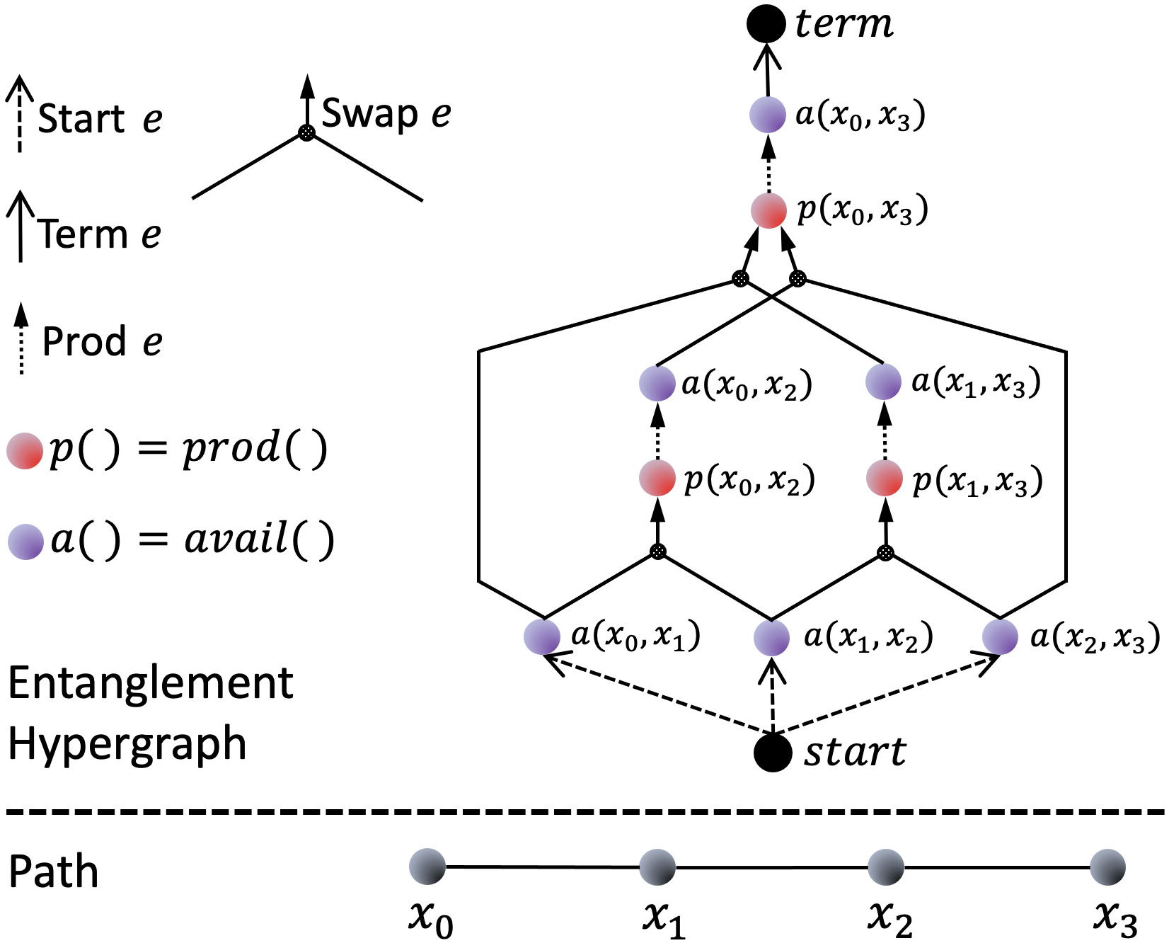
Figure 11: Entanglement hypergraph for a 4-node linear network. Not all $prod$ nodes are shown.

Entanglement Hypergraph. Given a QN and single $(s,d)$ pair, we first construct a hypergraph that represents the set of all possible swapping trees rooted at $(s,d)$. Given a QN represented as an undirected graph $G=(V,E)$ and a single $(s,d)$ pair, its entanglement hypergraph is a hypergraph $H$ constructed as follows (see Fig. 11). All pairs of vertices below are unordered pairs.

• $V(H)$ consists of:

  1. Two distinguished vertices $\mathit{start}$ and $\mathit{term}$

  2. $\mathit{prod}(u,v)$ and $\mathit{avail}(u,v)$ for all distinct $u,v\in V$

• $\mathit{E(H)}$ consists of 5 types of hyperarcs:

  1. [Start] $e=(\{\mathit{start}\},\{\mathit{avail}(u,v)\})\ \ \forall u,v\in V$.

  2. [Swap] $e=(\{\mathit{avail}(u,w),\mathit{avail}(w,v)\},\{\mathit{prod}(u,v)\})$, for all distinct $u,v,w\in V$.

  3. [Prod] $e=(\{\mathit{prod}(u,v)\},\{\mathit{avail}(u,v)\})\ \ \forall u,v\in V$.

  4. [Term] $e=(\{\mathit{avail}(s,d)\},\{\mathit{term}\})$.

In an entanglement hypergraph, vertices $\mathit{start}$ and $\mathit{term}$ represent source and sink nodes of a desired hypergragh-flow (see below). Other vertices represent EPs over a pair of nodes in $G$. Hyperarcs represent how the tail EPs contribute to that at the head. For ease of accounting, we categorize generated EPs using different types of vertices: $\mathit{start}$ represents link-level EPs generated over links in $G$, $\mathit{prod}$ represent EPs produced by atomic entanglement-swapping, and $\mathit{avail}$ represent EPs generated from either of the above. “Start” and “Prod” arcs turn the $\mathit{start}$ and $\mathit{prod}$ EPs respectively into $\mathit{avail}$ EPs and thus make them available for further swapping. “Swap” arcs represent swapping over the triplets of nodes $(u,w,v)$. Note that an entanglement hypergraph is a $B$-hypergraph, as “Swaps” are the only non-trivial hyperarcs, and their head is singleton.

Swapping Trees as $B$-Hyperpaths. Given a QNR problem with a single pair $(s,d)$, it is easy to see that any swapping tree generating $(s,t)$ EPs can be represented by a unique $B$-hyperpath from start to term in the above entanglement hypergraph. Thus, it easily follows that a QNR problem of selection of (multiple) swapping trees is equivalent to finding an optimal hypergraph flow from $\mathit{start}$ to $\mathit{term}$ in $H$. Note that $H$ has $O(|V|^{2})$ vertices and $O(|V^{3}|)$ hyperarcs.

A.2 Entanglement Flow as LP

We now develop an LP formulation to represent the QNR problem over $(s,d)$ in $G$ as a hypergraph-flow problem in $H$. In contrast to the classic hypergraph-flow formulation [2], we need to consider lossy flow, with loss arising from two sources: (i) ES operations have a given success probability, and (ii) waiting for both qubits to arrive before performing ES leads to losses since the arrival of EPs follow independent probability distributions. For the latter, we make use of Observation 1. The proposed LP formulation is as follows.

• Variables: $z_{a}$, for each hyperarc $a$ in $H$, represents the EP generation rate over each of the (one or two) node-pairs in $a$’s tail. This enforces the condition that EP rates over the two node-pairs in $\mathit{prod}$ hyperarc’s tail are equal. Thus, the LP solution will result in throttled swapping trees.

• Capacity Constraints: $z_{a}\in R^{+}$ for all hyperarcs $a$ in $H$. We use Eqn 2 to add the following constraints due to nodes in $G$.

  $$1/\mbox{$t_{g}$} \geq \sum_{x\in E(i)}z_{a(x)}/(\mbox{$p_{g}$}^{2}\mbox{$p_{e}$}^{2}\mbox{$p_{ob}$})\quad\forall i\in V.$$

  Above $a(x)$ is the hyperarc in $H$ of the form $(\mathit{start},\mathit{avail}(x))$ where $x$ is an edge in $G$.

• Flow Constraints which vary with vertex types. Below, we use notations $\mathit{out}(v)$ and $\mathit{in}(v)$ to represent outgoing and incoming hyperarcs from $v$. Formally, $\mathit{out}(v)$ is $\{a\in E(H):v\in t(a)\}$ and $\mathit{in}(v)$ is $\{a\in E(H):v\in h(a)\}$.

  • For each vertex $v$ s.t. $v=\mathit{avail}(\cdot)$:

    $$\sum_{a\in\mathit{in}(v)}z_{a}=\sum_{a^{\prime}\in\mathit{out}(v)}z_{a^{\prime}}$$

    That is, there is no loss in making already generated entanglements available for further swapping.

  • For each vertex $v$ s.t. $v=\mathit{prod}(\cdot)$:

    $$\sum_{a\in\mathit{in}(v)}z_{a}\mbox{$p_{b}$}(2/3)=\sum_{a^{\prime}\in\mathit{out}(v)}z_{a^{\prime}}$$

    The $(2/3)\mbox{$p_{b}$}$ factor follows from Observation 1, and accounts for loss due to swapping failures as well as due to waiting for arrival of both EPs for swapping.

• Objective: Maximize $\sum_{a\in\mathit{in}(\mathit{term})}z_{a}$

Multiple-Pairs Multi-Path: The above LP formulation for the single-pair QNR problem can be readily extended to the multiple-pairs case. Let $\{(s_{1},d_{1}),(s_{2},d_{2}),\ldots,(s_{n},d_{n})\}$ be a set of source-destination pairs. The only change is that the hypergraph $H$ now has $n$ arcs $(\{\mathit{avail}(s_{i},d_{i})\},\{\mathit{term}\})$ for all $i$. The other arcs model the generation of EPRs independent of the pairs, and thus are unchanged. It is interesting to note that the multi-pairs problem, typically formulated as multi-commodity flow in classical networks, is posed here as single-commodity flow over hypergraphs.

A.3 Fidelity

Constraints on loss of fidelity due to noisy BSM operations and from decoherence due to the age of qubits can be added to the LP formulation, as follows. Recall that constraint on operation-based fidelity loss is modelled by limiting the number leaves of the swapping tree, and in §4.2, we formulated the decoherence constraint by limiting the heights of the left-most and right-most descendants of the root’s children. These structural constraints on swapping trees can be lifted to the LP formulation by adding the leaf count and heights as parameters to $\mathit{prod}$ and $\mathit{avail}$ vertices; and (ii) swapping the EPs generated from only the compatible vertices.

In particular, we generalize the entanglement hypergraph to a fidelity-constrained one called $H^{(F)}$, where the $\mathit{prod}$ and $\mathit{avail}$ vertices are parameterized by $u,v\in V$, and in addition by $(n,h)$ where $n$ is the number of leaves and $h=(h_{ll},h_{lr},h_{rl},h_{rr})$ represents the depths of left-most and right-most descendants of the root’s children, of the trees rooted at $(u,v)$ with those parameter values. In terms of edges, the most interesting difference $H^{(F)}$ and $H$ is in “Swap” edges. In $H^{(F)}$, “Swap” edges are $(\{\mathit{avail}(u,w,n^{\prime},h^{\prime})$ $\mathit{avail}(w,v,n^{\prime\prime},h^{\prime\prime})\},$ $\{\mathit{prod}(u,v,n,h)\})$ only if $n=n^{\prime}+n^{\prime\prime}$, and $h,h^{\prime},h^{\prime\prime}$ are such that $h_{ll}=h^{\prime}_{ll}+1$, $h_{lr}=h^{\prime}_{rr}+1$, $h_{rl}=h^{\prime\prime}_{ll}+1$ and $h_{rr}=h^{\prime\prime}_{rr}+1$. The above constraints ensure that only compatible subtrees are composed into bigger trees. The other changes are for bookkeeping: “Gen” are from $\mathit{gen}(u,v)$ to $\mathit{avail}(u,v,1,(0,0,0,0))$; “Prod” are from $\mathit{prod}(u,v,n,h)$ to $\mathit{avail}(u,v,n,h)$; and finally “Term” are from $\mathit{avail}(s,t,n,h)$ to $\mathit{term}$ for $n\leq\tau_{l}$ and $h$ such that $f(h)\leq\tau_{d}$; here, $f(h)$ gives the tree’s age based on $h$ values (following §4.2) while using the link rates based on 50% node-capacity usage.

Table 1: Execution times of QNR-SP algorithm over small networks

Algorithm	Number of nodes
	10	13	15	16	18	20
Balanced-Tree	239$\mu$s	360$\mu$s	373$\mu$s	492$\mu$s	530$\mu$s	552$\mu$s
DP-Approx	4ms	10ms	14.7ms	17.6ms	28ms	34ms
DP-OPT	148ms	363ms	572ms	706ms	1s	1.7s
Caleffi [8]	92ms	4.6s	14s	26mins	3.2hrs	12.8hrs

Appendix B Proof of Theorem 1

Proof (sketch): We provide a main intuition behind the claim in Theorem 1. The key claim is that at any instant the WaitLess protocol generates an EP, the Waiting protocol will also be able to generate an EP. Consider an instant $t$ in time when the WaitLess protocol $X$ generates an EP, as a result of all the underlying processes succeeding at time $t$. Right before time $t$, consider the state of the EPs in the swapping-tree $T$ of the Waiting protocol $Y$: Essentially, some of the nodes in $T$ have (generated) EPs that are waiting for their sibling EP to be generated; note that these generated EPs have not aged yet, else they would have been already discarded by $Y$. Now, at time $t$, during $X$’s execution, all the underlying processes succeed instantly—it is easy to see that in the protocol $Y$ too, all the un-generated EP would now be generated instantly—yielding a full EP at the root (using qubits that have not aged beyond the threshold). Finally, since the number of operations in $T$ is the same as the number of BSM operations incurred by $X$ to generate an EP, the fidelity degradation due to operations is the same in both the protocols.

Appendix C Proof of Lemma 1

Proof. We first prove the claim that given any swapping tree $\mathcal{T}_{xy}$ over a path $P:x\leadsto w\leadsto y$, there exists a swapping tree $\mathcal{T}_{xw}$ over a path $P^{\prime}:x\leadsto w$ such that $P^{\prime}$ is a subset of $P$ and generation latency of $\mathcal{T}_{xw}$ is less than that of $\mathcal{T}_{xy}$. This claim can be easily proved by induction as follows. Consider two cases: (i) $w$ is the root of $\mathcal{T}_{xy}$, in which case $T_{xw}$ is the left child of the root. (ii) $i$ and $w$ have a common ancestor $a$ that is other than the root of $\mathcal{T}_{xy}$. In this case, $a$ = $w$, and the subtree rooted at $a=w$ is the required $\mathcal{T}_{xw}$. (iii) The only common ancestor of $i$ and $w$ is the root $a$ of $\mathcal{T}_{xw}$, which is not $w$. In this case, we apply the inductive hypothesis on right subtree $\mathcal{T}_{ay}$ of $\mathcal{T}_{xy}$, to extract a subtree $\mathcal{T}_{aw}$ which along with the left right subtree $\mathcal{T}_{ia}$ of $\mathcal{T}_{xy}$ — gives the required subtree $\mathcal{T}_{xw}$. This proves the above claim.

Now, to prove the lemma, let us consider the swapping trees $\mathcal{T}_{ik}$ and $\mathcal{T}_{kj}$ given to us. By the above claim, there are swapping trees $\mathcal{T}_{iv}$ and $\mathcal{T}_{vj}$, which will satisfy the requirements of the given lemma’s claim.

Appendix D Execution Times of Caleffi [8] Algorithm

Here, we give execution times of different algorithms especially Caleffi’s for small networks of 10-20 nodes. See Table 1. We see that Balanced-Tree and DP-Approx take fractions of a second, while DP-OPT takes upto 2 seconds. However, as expected Caleffi’s execution time increases exponentially with increase in number of nodes – with 20-node network takes 10+ hours. Below, we further estimate Caleffi’s execution time for larger graphs.

Rough Estimate of Caleffi’s Execution Time for Large Graphs. Consider a $n$-node network with an average node-degree of $d$. Consider a node pair $(s,d)$. We try to estimate the number of paths from $s$ to $d$ – the goal here is merely to show that the number is astronomical for $n$ = 100, and thus, our analysis is very approximate (more accurate analysis seems beyond the scope of this work). Let $P(l)$ be the number of simple paths from $s$ to a node $x$ in the graph of length at most $l$. For large graphs and large $l$, we can assume $P(l)$ to be roughly same for all $x$. We estimate that $P(l+1)=P(l)+P(l)*6*(1-l/n)$. The first term is to count paths of length at most $l-1$; in the second term, the factor 6 comes from the fact the destination $x$ has 6 neighbors and the factor $(1-l/n)$ is the probability that a path counted in $P(l)$ doesn’t contain $x$ (to constrain the paths to be simple, i.e,. without cycles). Using $P()$, the execution time of Caleffi can be roughly estimated to be at least $P(n-1)*500/(5*10^{9})$ seconds where the factor 500 is a conservative estimate of the number of instructions used in computing the latency for a path and $5*10^{9}$ is the number of instructions a 5GHz machine can execute in a second. The above yields executions times of a few seconds for $n=15$, about an hours for $n=20$, about 350 hours for $n=25$, and $10^{16}$ hours for $n=50$, and $10^{44}$ hours for $n=100$. The above estimates for $n=15$ to 20 are within an order of magnitude of our actual execution times, and thus, validate our estimation approach.

Appendix E Comparison with Caleffi: More Details

Fig. 8 shows that DP-OPT outperforms Caleffi by a margin of around 10% when averaging multiple experiments. However, when we look at one experiment at a time and compute the Caleffi’s performance relative to DP-OPT for each experiment, we see a larger difference between DP-OPT and Caleffi. Fig. 12 plots the error bar of the relative performance of three algorithms comparing to DP-OPT at each experiment. The lower cap of Caleffi at 0.2 atomic BSM success rate is 0.35, which means that at an extreme sample, the DP-OPT is almost 300% better than Caleffi. In that extreme sample, the number of hops between the source and destination is large (thus the overall EP rate is small, which affects little when averaging with other experiments in Fig. 8). Moreover, we observe that the larger number of hops between the source and destination, the larger the gap of relative performance is between DP-OPT and Caleffi. This observation aligns with what is shown in Fig. 6(b): our DP-OPT has an larger advantage in ratio when the source and destination are far away.

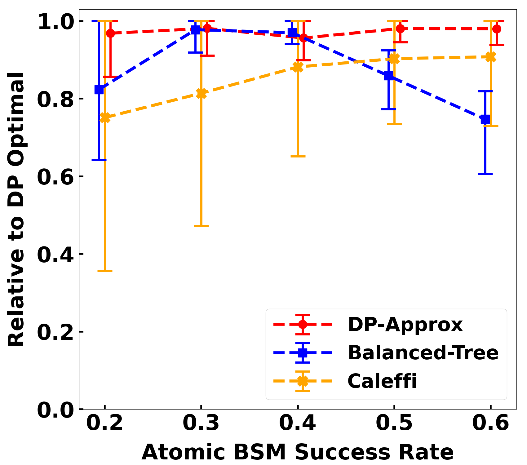
Figure 12: Compare the performance with Caleffi relative to DP-OPT (the closer to 1 the better).

Appendix F Execution Times Plot

We give here the plot for execution times of various schemes. See Fig. 13.

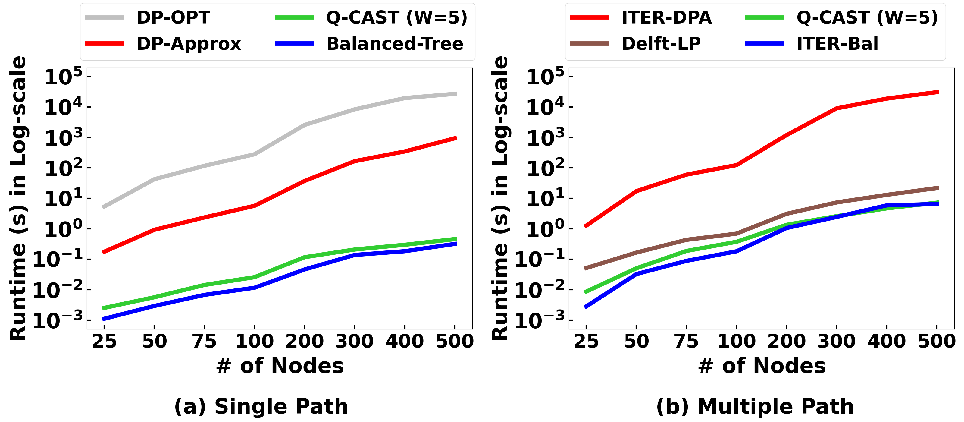
Figure 13: The execution time comparison of various algorithms for QNR-SP and QNR algorithms.

References

- [1] F. Arute et al. Quantum supremacy using a programmable superconducting processor. Nature, 574:505––510, 2019.
- [2] Isabel Beckenbach. Matchings and Flows in Hypergraphs. PhD thesis, Freie Universit at, Berlin, 2019.
- [3] C. H. Bennett, G. Brassard, C. Crépeau, R. Jozsa, A. Peres, and W. K. Wootters. Teleporting an unknown quantum state via dual classical and Einstein–Podolsky–Rosen channels. Phys. Rev. Lett., 70(13):1895––1899, 1993.
- [4] Charles H. Bennett, Gilles Brassard, Sandu Popescu, Benjamin Schumacher, John A. Smolin, and William K. Wootters. Purification of noisy entanglement and faithful teleportation via noisy channels. Physical Review Letters, 1996.
- [5] Charles H. Bennett, David P. DiVincenzo, John A. Smolin, and William K. Wootters. Mixed-state entanglement and quantum error correction. Physical Review A, 1996.
- [6] H.-J. Briegel, W. Dür, J. I. Cirac, and P. Zoller. Quantum repeaters: The role of imperfect local operations in quantum communication. Phys. Rev. Lett., 81:5932–5935, Dec 1998.
- [7] M. Caleffi, A. S. Cacciapuoti, and G. Bianchi. Quantum internet: from communication to distributed computing! https://arxiv.org/abs/1805.04360, 2018.
- [8] Marcello Caleffi. Optimal routing for quantum networks. IEEE Access, 2017.
- [9] Kaushik Chakraborty, David Elkouss, Bruno Rijsman, and Stephanie Wehner. Entanglement distribution in a quantum network: A multicommodity flow-based approach. IEEE Transactions on Quantum Engineering, 2020.
- [10] Kaushik Chakraborty, Filip Rozpedek, Axel Dahlberg, and Stephanie Wehner. Distributed routing in a quantum internet, 2019. https://arxiv.org/abs/1907.11630.
- [11] Teng-Yun Chen, Hao Liang, Yang Liu, Wen-Qi Cai, Lei Ju, Wei-Yue Liu, Jian Wang, Hao Yin, Kai Chen, Zeng-Bing Chen, et al. Field test of a practical secure communication network with decoy-state quantum cryptography. Optics express, 17(8):6540–6549, 2009.
- [12] Tim Coopmans, Robert Knegjens, Axel Dahlberg, David Maier, Loek Nijsten, Julio Oliveira, Stephanie Wehner, et al. Netsquid, a discrete-event simulation platform for quantum networks. arXiv preprint arXiv:2010.12535, 2020.
- [13] Axel Dahlberg, Matthew Skrzypczyk, Tim Coopmans, Leon Wubben, et al. A link layer protocol for quantum networks. In SIGCOMM, 2019.
- [14] Wenhan Dai, Tianyi Peng, and Moe Z. Win. Optimal remote entanglement distribution. IEEE Journal on Selected Areas in Communications, 38(3):540–556, 2020.
- [15] D. Dieks. Communication by EPR devices. Physics Letters A, 92(6):271–272, November 1982.
- [16] L-M Duan, Mikhail D Lukin, J Ignacio Cirac, and Peter Zoller. Long-distance quantum communication with atomic ensembles and linear optics. Nature, 2001.
- [17] Zachary Eldredge, Michael Foss-Feig, Jonathan A Gross, Steven L Rolston, and Alexey V Gorshkov. Optimal and secure measurement protocols for quantum sensor networks. Physical Review A, 97(4):042337, 2018.
- [18] E. Fraval, M. J. Sellars, and J. J. Longdell. Dynamic decoherence control of a solid-state nuclear-quadrupole qubit. Phys. Rev. Lett., 2005.
- [19] G. Gallo, G. Longo, S. Pallottino, and S. Nguyen. Directed hypergraphs and applications. Discrete Applied Mathematics, 42(2):177––201, 1993.
- [20] J. Gambetta. IBM’s Roadmap For Scaling Quantum Technology. https://www.ibm.com/blogs/research/2020/09/ibm-quantum-roadmap/, 2020.
- [21] Liang Jiang, Jacob M. Taylor, Navin Khaneja, and Mikhail D. Lukin. Optimal approach to quantum communication using dynamic programming. Proceedings of the National Academy of Sciences, 104(44):17291–17296, 2007.
- [22] Peter Komar, Eric M Kessler, Michael Bishof, Liang Jiang, Anders S Sørensen, Jun Ye, and Mikhail D Lukin. A quantum network of clocks. Nature Physics, 10(8):582–587, 2014.
- [23] Wojciech Kozlowski, Axel Dahlberg, and Stephanie Wehner. Designing a quantum network protocol. In CoNEXT, 2020.
- [24] J. J. Longdell, E. Fraval, M. J. Sellars, and N. B. Manson. Stopped light with storage times greater than one second using electromagnetically induced transparency in a solid. Phys. Rev. Lett., 2005.
- [25] Marco Marcozzi and Leonardo Mostarda. Quantum consensus: an overview. arXiv preprint arXiv:2101.04192, 2021.
- [26] Sreraman Muralidharan, Linshu Li, Jungsang Kim, Norbert Lütkenhaus, Mikhail D. Lukin, and Liang Jiang. Optimal architectures for long distance quantum communication. Scientific Reports, 6, 2016. https://doi.org/10.1038/srep20463.
- [27] Mihir Pant, Hari Krovi, Don Towsley, Leandros Tassiulas, Liang Jiang, Prithwish Basu, Dirk Englund, and Saikat Guha. Routing entanglement in the quantum internet. NPJ Quantum Information, 2020.
- [28] Joschka Roffe. Quantum error correction: an introductory guide. Contemporary Physics, 60(3):226–245, Jul 2019.
- [29] Kamyar Saeedi, Stephanie Simmons, Jeff Z Salvail, Phillip Dluhy, Helge Riemann, Nikolai V Abrosimov, Peter Becker, Hans-Joachim Pohl, John JL Morton, and Mike LW Thewalt. Room-temperature quantum bit storage exceeding 39 minutes using ionized donors in silicon-28. Science, 342(6160):830–833, 2013.
- [30] Nicolas Sangouard, Christoph Simon, Hugues De Riedmatten, and Nicolas Gisin. Quantum repeaters based on atomic ensembles and linear optics. Reviews of Modern Physics, 2011.
- [31] Valerio Scarani, Helle Bechmann-Pasquinucci, Nicolas J Cerf, Miloslav Dušek, Norbert Lütkenhaus, and Momtchil Peev. The security of practical quantum key distribution. Reviews of modern physics, 81(3):1301, 2009.
- [32] Shouqian Shi and Chen Qian. Concurrent entanglement routing for quantum networks: Model and designs. In SIGCOMM, 2020.
- [33] Christoph Simon. Towards a global quantum network. Nature Photonics, 11(11):678–680, 2017.
- [34] M Steger, K Saeedi, MLW Thewalt, JJL Morton, H Riemann, NV Abrosimov, P Becker, and H-J Pohl. Quantum information storage for over 180 s using donor spins in a 28si “semiconductor vacuum”. Science, 336(6086):1280–1283, 2012.
- [35] M. Thakur and R. Tripathi. Linear connectivity problems in directed hypergraphs. Theoretical Computer Science, 410(27):2592––2618, 2009.
- [36] W. Tittel, M. Afzelius, R. L. Cone, T. Chanelière, S. Kröll, S. A. Moiseev, and M. Sellars. Photon-echo quantum memory, 2008. https://arxiv.org/abs/0810.0172.
- [37] Pengfei Wang, Chun-Yang Luan, Mu Qiao, Mark Um, Junhua Zhang, Ye Wang, Xiao Yuan, Mile Gu, Jingning Zhang, and Kihwan Kim. Single ion qubit with estimated coherence time exceeding one hour. Nature Communications, 12(1), Jan 2021.
- [38] B.M. Waxman. Routing of multipoint connections. IEEE Journal on Selected Areas in Communications, 1988.
- [39] William K Wootters and Wojciech H Zurek. A single quantum cannot be cloned. Nature, 299(5886):802–803, 1982.
- [40] Manjin Zhong, Morgan P Hedges, Rose L Ahlefeldt, John G Bartholomew, Sarah E Beavan, Sven M Wittig, Jevon J Longdell, and Matthew J Sellars. Optically addressable nuclear spins in a solid with a six-hour coherence time. Nature, 517(7533):177–180, 2015.