A deterministic–particle–based scheme for micro-macro viscoelastic flows

Abstract

In this article, we introduce a new method for discretizing micro-macro models of dilute polymeric fluids based on deterministic particles. Our approach integrates a finite element discretization for the macroscopic fluid dynamic equation with a deterministic variational particle scheme for the microscopic Fokker-Planck equation. To address challenges arising from micro-macro coupling, we employ a discrete energetic variational approach to derive a coarse-grained micro-macro model with a particle approximation first and then develop a particle-FEM discretization for the coarse-grained model. The accuracy of our method is evaluated for a Hookean dumbbell model in a Couette flow by comparing the computed velocity field with existing analytical solutions. We also use our method to study nonlinear FENE dumbbell models in different scenarios, such as extension flow, pure shear flow, and lid-driven cavity flow. Numerical examples demonstrate that the proposed deterministic particle approach can accurately capture the various key rheological phenomena in the original FENE model, including hysteresis and $\delta$-function-like spike behavior in extension flows, velocity overshoot phenomenon in pure shear flow, symmetries breaking, vortex center shifting and vortices weakening in the lid-driven cavity flow, with a small number of particles.

1 Introduction

Complex fluids comprise a large class of soft materials, such as polymeric solutions, liquid crystals, ionic solutions, and fiber suspensions. These are fluids with complicated rheological phenomena, arising from different “elastic” effects, such as elasticity of deformable particles, interaction between charged ions and bulk elasticity endowed by polymer molecules [45]. Modeling and simulations of complex fluids have been interesting problems for a couple of decades [7, 39, 12, 41].

Models for complex fluids are typically categorized as pure macroscopic models [35, 42, 61] and micro-macro models [8, 12]. The pure macroscopic models employ an empirical constitutive equation for the stress tensor ${\bm{\tau}}$ to supplement the conservation laws of mass and momentum [35, 42, 61]. Examples include Oldroyd-B model [51] and FENE-P model [56]. This approach is advantageous due to its low computational cost, but the closed-form of the constitutive equation may fail to capture the intricate flow behaviors of complex fluids, including hysteresis effects. Micro-macro models, on the other hand, couple macroscopic conservation laws with microscopic kinetic theory, which describes the origin of the macroscopic stress tensor [8, 12]. The approach gives an elegant description to the origin of the macroscopic stress tensor for various complex fluids [8, 12, 44]. However, directly simulating micro-macro models has been a long-standing challenge.

The goal of this paper is to develop an efficient numerical method for micro-macro models. To clarify our approach, we will focus on a simple micro-macro model of dilute polymeric fluids. In this model, a polymer chain is represented by an elastic dumbbell consisting of two beads connected by a single spring at the microscopic level. The molecular configuration is characterized by an end-to-end vector of the dumbbell, represented by $\bm{q}\in\mathbb{R}^{d}$. The macroscopic motion of the fluid is described by a Navier–Stokes equation with elastic stress ${\bm{\tau}}$ induced by the microscopic configuration of polymer chains. The microscopic dynamics is modeled using a Fokker-Planck equation for the number density distribution function $f(\bm{x},\bm{q},t)$ with a drift term depending on the macroscopic velocity field $\bm{u}$. The corresponding micro-macro model is formulated as follows:

$$\left\{\begin{aligned} &\rho(\bm{u}_{t}+\bm{u}\cdot\nabla\bm{u})+\nabla p=\eta_{s}\Delta\bm{u}+\nabla\cdot{\bm{\tau}},\\ &{\bm{\tau}}=\lambda_{p}\mathbb{E}(\nabla_{\bm{q}}\Psi\otimes\bm{q})=\lambda_{p}\int_{\mathbb{R}^{d}}f\nabla_{\bm{q}}\Psi\otimes\bm{q}d\bm{q},\\ &\nabla\cdot\bm{u}=0,\\ &f_{t}+\bm{u}\cdot\nabla f+\nabla_{\bm{q}}\cdot((\nabla\bm{u})\bm{q}f)=\frac{2}{\zeta}\nabla_{\bm{q}}\cdot(f\nabla_{\bm{q}}\Psi)+\frac{2k_{B}T}{\zeta}\Delta_{\bm{q}}f\ ,\end{aligned}\right.$$ (1)

where $\rho$ is the constant density of the fluid, $\lambda_{p}$ is a constant that represents the polymer density, $k_{B}$ is the Boltzmann constant, $T$ is the absolute temperature, $\eta_{s}$ is the solvent viscosity, $\zeta$ is a constant related to the polymer relaxation time, and $\Psi(\bm{q})$ is the spring potential. In Hookean and FENE (Finite Extensible Nonlinear Elastic) models, the elastic potential $\Psi(\bm{q})$ is given by

$$\Psi(\bm{q})=\frac{1}{2}H|\bm{q}|^{2},\quad\text{and}\quad\Psi(\bm{q})=-\frac{HQ_{0}^{2}}{2}\ln\bigg{(}1-\bigg{(}\frac{|\bm{q}|}{Q_{0}}\bigg{)}^{2}\bigg{)},$$

respectively, where $H>0$ is the elastic constant, $Q_{0}$ is the maximum dumbbell extension in FENE models. The interactions among polymer chains are neglected due to the dilute assumption. Alternatively, the microscopic dynamics can also be described by a stochastic differential equation (SDE), or Langevin dynamics, given by [12]

$$\mathrm{d}\bm{q}(\bm{x},t) =\left(-\bm{u}\cdot\nabla\bm{q}(\bm{x},t)+(\nabla\bm{u})\bm{q}(\bm{x},t)-2\zeta^{-1}\nabla_{q}\Psi(\bm{q}(\bm{x},t))\right)\mathrm{d}t+\sqrt{4k_{B}T\zeta^{-1}}\mathrm{d}{\bf W}_{t},$$ (2)

where $\mathrm{d}{\bf W}_{t}$ is the standard multidimensional white noise.

In recent decades, various computational techniques have been developed to solve the micro-macro model (1)[22, 28, 30, 40, 50, 54]. The two main approaches are Langevin equation-based stochastic simulation methods and direct simulation methods based on the microscopic Fokker-Planck equation [50]. One of the earliest Langevin-based numerical methods is the CONNFFESSIT (Calculation of Non-Newtonian Flow: Finite Elements and Stochastic Simulation Technique) algorithm, which couples a finite element discretization to the macroscopic flow with a numerical solver for the microscopic SDE (2) [40, 54]. Along this direction, other stochastic approaches, such as the Lagrangian particle method (LPM) [28] and the Brownian configuration field (BCF) method [30], were proposed to reduce the variance and computational cost of the original CONNFFESSIT algorithm. Several extensions and corresponding numerical experiments have been extensively investigated in recent years [10, 12, 14, 25, 33, 37, 68]. Although stochastic approaches have been the dominant simulation methods for micro-macro models, they suffer from several shortcomings, including high computational cost and stochastic fluctuations. An alternative approach is the direct simulation of the equivalent Fokker-Planck equation in the configurational space. Examples include Galerkin spectral element technique [15, 36, 49, 60, 63] and the lattice Boltzmann technique [1, 6]. However, such methods are well suited only for polymeric models having low-dimensional configurational spaces, and the computational cost of Fokker-Planck-based methods increases rapidly for simulations in strong flows (with highly localized distribution function) or involving high-dimensional configuration spaces.

Deterministic particle methods have recently gained considerable attention in the context of solving Fokker-Planck type equations [59, 18, 38, 13, 65]. These methods handle the diffusion terms in the equation by using various kernel regularizations [13, 18, 38, 59]. Unlike Langevin dynamics-based stochastic particle methods, deterministic particle methods are often computationally cheap and do not suffer from stochastic fluctuations. The success of deterministic particle methods in solving Fokker-Planck equations has motivated us to develop an efficient numerical method for micro-macro models by incorporating a deterministic particle method. However, the micro-macro coupling in these models presents new challenges that need to be addressed. To overcome these difficulties, we apply the particle approximation at the energy-dissipation law level and employ a discrete energetic variational approach [46, 65] to derive a coarse-grained micro-macro model with a particle approximation first. A particle-FEM discretization is developed for the coarse-grained model. Various numerical experiments have been performed to validate the new scheme via several benchmark problems. Despite its simplicity, the deterministic particle method is robust, accurate and able to catch certain complex behaviors of polymeric fluids. The numerical results obtained by our scheme are in excellent agreement with those from the former work. Moreover, the deterministic particle discretization is shown to be more efficient than the stochastic particle approaches, where a large ensemble of realizations of the stochastic process are needed.

The rest of this article is organized as follows. A formal derivation of the micro-macro model of dilute polymeric fluids by employing the energetic variational approach is given in Section 2. Then we derive a coarse-grained micro-macro model with the particle approximation and construct the deterministic particle-FEM scheme in Section 3. Various numerical experiments are presented in Section 4. Finally, the concluding remarks are given in Section 5.

2 Energetic variational approach to the micro-macro model

In this section, we present a formal derivation of micro-macro models for dilute polymeric fluids using the energetic variational approach (EnVarA). This approach builds upon the works of Rayleigh [57] and Onsager [52, 53] on non-equilibrium thermodynamics, and has been successfully applied to build various mathematical models in physics, chemical engineering, and biology [24, 66]. The EnVarA framework utilizes a prescribed energy-dissipation law and a kinematic (transport) relation to derive the dynamics of a non-equilibrium thermodynamic system through the Least Action Principle (LAP) and the Maximum Dissipation Principle (MDP) [24]. From a numerical perspective, EnVarA also serves as a valuable guideline for developing structure-preserving numerical schemes for these complex systems [46].

More precisely, according to the first and second laws of thermodynamics [23, 24], an isothermal and closed system possesses an energy-dissipation law

$$\frac{\mathrm{d}}{\mathrm{d}t}E^{\text{total}}(t)=-\triangle(t)\leq 0\ .$$ (3)

Here $E^{\text{total}}$ is the total energy, which is the sum of the Helmholtz free energy $\mathcal{F}$ and the kinetic energy $\mathcal{K}$; $\triangle(t)\geq 0$ stands for the rate of energy dissipation, which equals to the entropy production in this case. Once these quantifies are specified, for the energy part, one can apply the LAP, taking variation of the action functional $\mathcal{A}(\bm{x})=\int_{0}^{T}\left(\mathcal{K}-\mathcal{F}\right)\mathrm{d}t$ with respect to $\bm{x}$ (the trajectory in Lagrangian coordinates) [2, 24], to derive the conservative force, i.e., $\delta\mathcal{A}=\int_{0}^{T}\int_{\Omega}({\rm force}_{\text{iner}}-{\rm force}_{\text{conv}})\cdot\delta\bm{x}\mathrm{d}\bm{x}\mathrm{d}t.$ For the dissipation part, one can apply the MDP, taking variation of the Onsager dissipation functional $\mathcal{D}$ with respect to the “rate” $\bm{x}_{t}$, to derive the dissipative force, i.e., $\delta\mathcal{D}=\int_{\Omega(t)}{\rm force}_{\text{diss}}\cdot\delta\bm{x}_{t}~{}\mathrm{d}\bm{x}$, where the dissipation functional $\mathcal{D}=\frac{1}{2}\triangle$ in the linear response regime [52]. Consequently, the force balance condition (Newton’s second law, in which the inertial force plays a role of $ma$) results in

$$\frac{\delta\mathcal{A}}{\delta\bm{x}}=\frac{\delta\mathcal{D}}{\delta\bm{x}_{t}},$$ (4)

which is the dynamics of the system.

As mentioned in the introduction, the micro-macro model (1) models polymer molecules as elastic dumbbells consisting of two ”beads” joined by a one-dimensional spring at the microscopic scale [41, 44]. The microscopic configuration between the two beads is described by an end-to-end vector ${\bm{q}}\in\mathbb{R}^{d}$. The number density distribution function of finding a molecule with end-to-end vector $\bm{q}$ at position $\bm{x}\in\Omega$ at time $t$ is denoted by $f(\bm{x},\bm{q},t)$.

To specify the kinematics of $f(\bm{x},\bm{q},t)$, Lagrangian descriptions are needed for both micro- and macro-scales. Let $\bm{x}(\mathbf{X},t)$ be the flow map in physical space and $\bm{q}(\mathbf{X},\bm{Q},t)$ be the flow map in configurational space, where $\bm{X}$ and $\bm{Q}$ are Lagrangian coordinates in physical and configurational space, respectively. For given flow maps $\bm{x}(\mathbf{X},t)$ and $\bm{q}(\mathbf{X},\bm{Q},t)$, the corresponding macroscopic velocity $\bm{u}$ and the microscopic velocity ${\bm{V}}$ satisfy

$$\bm{u}(\bm{x}(\mathbf{X},t),t)=\bm{x}_{t}(\mathbf{X},t),\quad{\bm{V}}(\bm{x}(\mathbf{X},t),\bm{q}(\mathbf{X},\bm{Q},t),t)=\bm{q}_{t}(\mathbf{X},\bm{Q},t)\ .$$ (5)

Moreover, one can define the deformation tensor associated with the flow map $\bm{x}(\mathbf{X},t)$ by

$${\sf\tilde{F}}(\bm{x}(\mathbf{X},t),t)={\sf F}(\mathbf{X},t)=\nabla_{\mathbf{X}}\bm{x}(\mathbf{X},t)\ .$$ (6)

Without ambiguity, in this paper, we will not distinguish ${\sf F}$ and ${\sf\tilde{F}}$. Obviously, ${\sf F}$ carries all the transport information of configurations in the system [43] and satisfies the transport equation in Eulerian coordinates [44]

$${\sf F}_{t}+\bm{u}\cdot\nabla{\sf F}=(\nabla\bm{u}){\sf F}\ .$$

Due to the conservation of mass, the density distribution function $f(\bm{x},\bm{q},t)$ satisfies

$$\frac{\mathrm{d}}{\mathrm{d}t}\int_{\Omega}\int_{\mathbb{R}^{d}}f(\bm{x},\bm{q},t)\mathrm{d}\bm{q}\mathrm{d}\bm{x}=0\ ,$$ (7)

which can be written as

$$\partial_{t}f+\nabla\cdot(f\bm{u})+\nabla_{\bm{q}}\cdot(f{\bm{V}})=0$$ (8)

in Eulerian coordinates. Here $\bm{u}(\bm{x},t)$ and ${\bm{V}}(\bm{x},\bm{q},t)$ are the macro- and microscopic velocities associated with the flow maps.

The micro-macro system can be modeled through an energy-dissipation law

$$\frac{\mathrm{d}}{\mathrm{d}t}\int_{\Omega}\bigg{(}\frac{1}{2}\rho|\bm{u}|^{2}+\lambda_{p}\int_{\mathbb{R}^{d}}k_{B}Tf\ln f+\Psi fd\bm{q}\bigg{)}d\bm{x}=-\int_{\Omega}\bigg{(}\eta_{s}|\nabla\bm{u}|^{2}+\int_{\mathbb{R}^{d}}\frac{\lambda_{p}\zeta}{2}f|{\bm{V}}-\widetilde{\mathbf{V}}|^{2}d\bm{q}\bigg{)}d\bm{x}\ ,$$ (9)

where $\rho$ is the constant density of the fluid, $\lambda_{p}$ is a constant that represents the polymer density, $k_{B}$ is the Boltzmann constant, $T$ is the absolute temperature, $\eta_{s}$ is the solvent viscosity, the constant $\zeta$ is related to the polymer relaxation time, $\Psi=\Psi(\bm{q})$ is the microscopic elastic potential of the polymer molecules. For Hookean and FENE models, the elastic potential $\Psi(\bm{q})$ is given by $\Psi(\bm{q})=\tfrac{1}{2}H|\bm{q}|^{2},$ and $\Psi(\bm{q})=-\tfrac{HQ_{0}^{2}}{2}\ln\left(1-\left(\tfrac{|\bm{q}|}{Q_{0}}\right)^{2}\right),$ respectively, where $H>0$ is the elastic constant, $Q_{0}$ is the maximum dumbbell extension in FENE models. The second term of the dissipation accounts for the micro-macro coupling with $\widetilde{\mathbf{V}}$ being the macroscopic induced velocity. According to the Cauchy-Born rule, $\bm{q}={\sf F}\bm{Q}$ at the macroscopic scale, which indicates

$$\widetilde{\mathbf{V}}=\frac{\mathrm{d}}{\mathrm{d}t}\bigg{(}{\sf F}\bm{Q}\bigg{)}=\bigg{(}\frac{\mathrm{d}}{\mathrm{d}t}{\sf F}\bigg{)}\bm{Q}=(\nabla\bm{u}{\sf F})\bm{Q}=(\nabla\bm{u})\bm{q}.$$

Next we derive the dynamics of the system by applying the LAP and MDP. First, we look at the dynamics at the macroscopic scale. Due to the “separation of scale” [24], the second term on the right hand side of the dissipation (9) vanishes when deriving the macroscopic force balance. Since $\det{\sf F}=1$, the action functional can be written as

$$\mathcal{A}(\bm{x})=\int_{0}^{T}\int_{\Omega_{0}}\bigg{[}\frac{1}{2}\rho|\bm{x}_{t}|^{2}-\lambda_{p}\int_{\mathbb{R}^{d}}k_{B}Tf_{0}\ln f_{0}+\Psi({\sf F}\bm{Q})f_{0}\mathrm{d}\bm{Q}\bigg{]}d\mathbf{X}dt$$ (10)

in Lagrangian coordinates, where $f_{0}(\mathbf{X},\bm{Q})$ is the initial number distribution function, and $f(\bm{x},{\sf F}\bm{Q},t)=f_{0}(\mathbf{X},\bm{Q})$ due to $\det{\sf F}=1$. By applying the LAP, i.e., taking variation of $\mathcal{A}(\bm{x})$ with respect to $\bm{x}$, we get

$$\frac{\delta\mathcal{A}}{\delta\bm{x}}=-\rho(\bm{u}_{t}+\bm{u}\cdot\nabla\bm{u})+\lambda_{p}\nabla\cdot\bigg{(}\int_{\mathbb{R}^{d}}f\nabla_{\bm{q}}\Psi\otimes\bm{q}d\bm{q}\bigg{)}$$ (11)

in Eulerian coordinates. Indeed, consider a perturbation $\bm{x}^{\epsilon}(\mathbf{X},t)=\bm{x}(\mathbf{X},t)+\epsilon\bm{y}(\mathbf{X},t),$ where $\bm{y}(\mathbf{X},t)=\tilde{\bm{y}}(\bm{x}(\mathbf{X},t),t)$ is the perturbation satisfying $\tilde{\bm{y}}\cdot{\bf n}=0$ with ${\bf n}$ being the outer normal of $\Omega$. Then

$$\frac{\mathrm{d}}{\mathrm{d}t}\mathcal{A}(\bm{x}^{\epsilon})\Big{|}_{\epsilon=0}=\int_{0}^{T}\int_{\Omega_{0}} \Bigl{[}-\rho\bm{x}_{tt}\cdot\bm{y}-\lambda_{p}\int_{\mathbb{R}^{d}}f_{0}\nabla_{\bm{q}}\Psi\otimes\bm{Q}:\nabla_{\mathbf{X}}\bm{y}\mathrm{d}\bm{Q}\Bigr{]}\mathrm{d}\mathbf{X}$$

Push forward to Eulerian coordinates, we have

$$\frac{\mathrm{d}}{\mathrm{d}t}\mathcal{A}(\bm{x}^{\epsilon})\Big{|}_{\epsilon=0}=\int_{0}^{T}\int_{\Omega}\Bigl{[}-\rho(\bm{u}_{t}+\bm{u}\cdot\nabla\bm{u})\cdot\tilde{\bm{y}}-\lambda_{p}\int_{\mathbb{R}^{d}}f\nabla_{\bm{q}}\Psi\otimes\bm{q}:\nabla_{\bm{x}}\tilde{\bm{y}})\mathrm{d}\bm{q}\Bigr{]}\mathrm{d}\bm{x}$$

$$=\int_{0}^{T}\int_{\Omega}\left(-\rho(\bm{u}_{t}+\bm{u}\cdot\nabla\bm{u})+\lambda_{p}\nabla\cdot(\int_{\mathbb{R}^{d}}f\nabla_{\bm{q}}\Psi\otimes\bm{q}\mathrm{d}\bm{q})\right)\cdot\tilde{\bm{y}}\mathrm{d}\bm{x},$$

which leads to (11). For the dissipation part, the MDP, i.e., taking variation of $\mathcal{D}$ with respect to $\bm{x}_{t}$, leads to

$$\frac{\delta\mathcal{D}}{\delta\bm{x}_{t}}=-\eta_{s}\Delta\bm{u}+\nabla p,$$ (12)

where $p$ is the Lagrangian multiplier for the incompressible condition $\nabla\cdot\bm{u}=0$. Hence, the macroscopic force balance results in the momentum equation

$$\rho(\bm{u}_{t}+\bm{u}\cdot\nabla\bm{u})+\nabla p=\eta_{s}\Delta\bm{u}+\nabla\cdot{\bm{\tau}},$$ (13)

where

$${\bm{\tau}}=\lambda_{p}\int_{\mathbb{R}^{d}}f\nabla_{\bm{q}}\Psi\otimes\bm{q}d\bm{q}$$ (14)

is the induced stress from the configuration space, representing the microscopic contributions to the macroscopic level. Here, $\otimes$ denotes a tensor product and $\bm{u}\otimes\mathbf{v}$ is a matrix $(u_{i}v_{j})$ for two vectors $\bm{u}$ and $\mathbf{v}$. The formula (14) is known as the Irving–Kirkwood formula or the Kramers’ expression for the induced stress [41].

On the microscopic scale, by taking variations with respect to $\bm{q}(\mathbf{X},\bm{Q},t)$ and ${\bm{V}}(\mathbf{X},\bm{Q},t)$ for the free energy and the dissipation parts, we obtain

$$\frac{\zeta}{2}({\bf V}-\nabla\bm{u}\bm{q})=-\nabla_{\bm{q}}(k_{B}T\ln f+1+\Psi).$$ (15)

Combining (15) with Eq. (8), we get the equation on the microscopic scale:

$$f_{t}+\nabla\cdot(\bm{u}f)+\nabla_{\bm{q}}\cdot(\nabla\bm{u}\bm{q}f)=\frac{2}{\zeta}\nabla_{\bm{q}}\cdot(f\nabla_{\bm{q}}\Psi)+\frac{2k_{B}T}{\zeta}\Delta_{\bm{q}}f.$$ (16)

And thus, the final coupled system reads as follows,

$$\left\{\begin{aligned} &\rho(\bm{u}_{t}+\bm{u}\cdot\nabla\bm{u})+\nabla p=\eta_{s}\Delta\bm{u}+\nabla\cdot\bm{\tau},\\ &\bm{\tau}=\lambda_{p}\int_{\mathbb{R}^{d}}f\nabla_{\bm{q}}\Psi\otimes\bm{q}d\bm{q},\\ &\nabla\cdot\bm{u}=0,\\ &f_{t}+\nabla\cdot(\bm{u}f)+\nabla_{\bm{q}}\cdot(\nabla\bm{u}\bm{q}f)=\frac{2}{\zeta}\nabla_{\bm{q}}\cdot(f\nabla_{\bm{q}}\Psi)+\frac{2k_{B}T}{\zeta}\Delta_{\bm{q}}f,\end{aligned}\right.$$ (17)

subject to a suitable boundary condition.

It is convenient to nondimensionalize the micro-macro model by introducing the following nondimensionalized parameters:

$${\rm Re}=\frac{\rho\tilde{U}\tilde{L}}{\eta},\quad{\rm Wi}=\frac{\lambda\tilde{U}}{\tilde{L}},\quad\tilde{\eta}_{s}=\frac{\eta_{s}}{\eta},\quad\epsilon_{p}=\frac{\eta_{p}}{\eta},\quad\lambda=\frac{\zeta}{4H},$$

where $\tilde{L}=\sqrt{\frac{k_{B}T}{H}}$ is the characteristic length scale, $\tilde{U}$ is the characteristic velocity, $\eta_{p}=\lambda_{p}k_{B}T\lambda$ is related to the polymer viscosity, $\eta$ is the total fluid viscosity and $\eta=\eta_{s}+\eta_{p}$. The final nondimensionalized system reads as follows,

$$\left\{\begin{aligned} &\mathrm{Re}(\bm{u}_{t}+\bm{u}\cdot\nabla\bm{u})+\nabla p=\tilde{\eta}_{s}\Delta\bm{u}+\nabla\cdot\bm{\tau},\\ &{\bm{\tau}}=\frac{\epsilon_{p}}{{\rm Wi}}\int f\nabla_{\bm{q}}\Psi\otimes\bm{q}\mathrm{d}\bm{q},\\ &\nabla\cdot\bm{u}=0,\\ &f_{t}+\nabla\cdot(\bm{u}f)+\nabla_{\bm{q}}\cdot(\nabla\bm{u}\bm{q}f)=\frac{1}{2\rm Wi}\nabla_{\bm{q}}\cdot(f\nabla_{\bm{q}}\Psi)+\frac{1}{2\rm Wi}\Delta_{\bm{q}}f,\end{aligned}\right.$$ (18)

where

$$\Psi(\bm{q})=\frac{1}{2}|\bm{q}|^{2},\qquad\nabla_{\bm{q}}\Psi=\bm{q},$$

in Hookean model, and

$$\Psi(\bm{q})=-\frac{b}{2}\ln(1-|\bm{q}|^{2}/b),\qquad\nabla_{\bm{q}}\Psi=\frac{\bm{q}}{1-|\bm{q}|^{2}/b}$$

with $b=HQ_{0}^{2}/k_{B}T$ in FENE model.

3 The deterministic particle-FEM method

In this section, we construct the numerical scheme for the micro-macro model (17), which combines a finite element discretization of the macroscopic fluid dynamic equation [4, 5, 16] with a deterministic particle method for the microscopic Fokker-Planck equation [65]. To overcome the difficulty arising from micro-macro coupling, we first employ a discrete energetic variational approach to derive a particle–based micro–macro model. The discrete energetic variational approach follows the idea of “Approximation-then-Variation”, which first applies particle approximation to the continuous energy dissipation law. As an advantage, the derived coarse-grained system preserves the variational structure at the particle level.

3.1 A discrete energetic variational approach

For simplicity, we assume that

$$\int_{\mathbb{R}^{d}}f(\bm{x},\bm{q},t)\mathrm{d}\bm{q}=1,\quad\forall\bm{x}\in\Omega,$$ (19)

which means that the number density of polymer chains is spatially homogeneous. Thus, for fixed $\bm{x}$, $f(\bm{x},\bm{q},t)$ can be approximated by

$$f(\bm{x},\bm{q},t)\approx f_{N}(\bm{x},\bm{q},t)=\sum_{i=1}^{N}\omega_{i}(\bm{x},t)\delta(\bm{q}-\bm{q}_{i}(\bm{x},t)),\quad\forall\bm{x}\in\Omega\ ,$$ (20)

where $N$ is the number of particles at $\bm{x}$ and time $t$, $\{\bm{q}_{i}(\bm{x},t)\}_{i=1}^{N}$ is a set of particles at $\bm{x}$ and time $t$, $\omega_{i}(\bm{x},t)$ is the weight of the corresponding particle satisfying $\sum_{i=1}^{N}\omega_{i}(\bm{x},t)=1$. In the current work, we fix $\omega_{i}(\bm{x},t)=\frac{1}{N}$, i.e., all the particles are equally weighted.

Remark 3.1.

$\{\bm{q}_{i}(\bm{x},t)\}_{i=1}^{N}$ can be viewed as representative particles that represent information of the number density distribution $f(\bm{x},\bm{q},t)$ at $\bm{x}$. Since only $\bm{q}_{i}(\bm{x},t)$ needs to be computed at each time-step, the computational cost can be largely reduced, compared to computing $f(\bm{x},\bm{q},t)$.

Substitute the approximation (20) into the continuous energy-dissipation law (9), we can obtain a discrete energy-dissipation law in terms of $\bm{q}_{i}(\bm{x},t)$ and the macroscopic flow. Notice that the term $\ln f_{N}(\bm{x},\bm{q},t)$ can not be defined in a proper way, we introduce a kernel regularization, i.e., replacing $\ln f_{N}$ by $\ln(K_{h}\ast f_{N})$ [13], where $K_{h}$ is a kernel function and

$$K_{h}\ast f_{N}(:,\bm{q},:)=\int K_{h}(\bm{q}-\bm{p})f_{N}(:,\bm{p},:)\mathrm{d}{\bm{p}}=\frac{1}{N}\sum_{j=1}^{N}K_{h}(\bm{q}-\bm{q}_{j}(\bm{x},t)).$$

A typical choice of $K_{h}$ is the Gaussian kernel, given by

$$K_{h}(\bm{q}_{1},\bm{q}_{2})=\frac{1}{(\sqrt{2\pi}h_{p})^{d}}\exp\left(-\frac{|\bm{q}_{1}-\bm{q}_{2}|^{2}}{2h_{p}^{2}}\right).$$

Here $h_{p}$ is the kernel bandwidth which controls the inter-particle distances and $d$ is the dimension of the space. We take $h_{p}$ as a constant for simplicity. The values of $h_{p}$ will affect the numerical results. We’ll discuss the choices of $h_{p}$ in the next section.

Within the kernel regularization, the discrete energy can be written as

$$\mathcal{F}_{h}\left[\{\bm{q}_{i}\}_{i=1}^{N},\bm{x}\right] =\int_{\Omega}\frac{1}{2}\rho|\bm{u}|^{2}+\lambda_{p}\frac{1}{N}\sum_{i=1}^{N}\left[k_{B}T\ln\left(\frac{1}{N}\sum_{j=1}^{N}K_{h}(\bm{q}_{i}-\bm{q}_{j})\right)+\Psi(\bm{q}_{i})\right]\mathrm{d}\bm{x},$$ (21)

and the discrete dissipation is

$$-2\mathcal{D}_{h}\left[\{\bm{q}_{i}\}_{i=1}^{N},\{\dot{\bm{q}}_{i}\}_{i=1}^{N},\bm{x},\bm{u}\right]=-\int_{\Omega}\eta_{s}|\nabla\bm{u}|^{2}+\frac{\lambda_{p}\zeta}{2}\frac{1}{N}\sum_{i=1}^{N}|\dot{\bm{q}}_{i}-\nabla\bm{u}\bm{q}_{i}|^{2}\mathrm{d}\bm{x},$$ (22)

where $\dot{\bm{q}_{i}}=\partial_{t}\bm{q}_{i}+\bm{u}\cdot\nabla\bm{q}_{i}$ is the material derivative of $\bm{q}_{i}$, $(\nabla\bm{u})\bm{q}_{i}$ is the velocity of particle induced by the macroscopic flow due to the Cauchy-Born rule. The dynamics of $\bm{q}_{i}(\bm{x},t)$ can be derived by performing the EnVarA in terms of $\bm{q}_{i}$ and $\dot{\bm{q}_{i}}$, i.e.,

$$\frac{\delta\mathcal{D}_{h}}{\delta\dot{\bm{q}}_{i}}=-\frac{\delta\mathcal{F}_{h}}{\delta\bm{q}_{i}},$$

which leads to

$$\dot{\bm{q}_{i}} =(\nabla\bm{u})\bm{q}_{i}-\frac{2}{\zeta}\bigg{[}k_{B}T\bigg{(}\frac{\sum_{j=1}^{N}\nabla_{\bm{q}_{i}}K_{h}(\bm{q}_{i},\bm{q}_{j})}{\sum_{j=1}^{N}K_{h}(\bm{q}_{i},\bm{q}_{j})}+\sum_{k=1}^{N}\frac{\nabla_{\bm{q}_{i}}K_{h}(\bm{q}_{k},\bm{q}_{i})}{\sum_{j=1}^{N}K_{h}(\bm{q}_{k},\bm{q}_{j})}\bigg{)}+\nabla_{\bm{q}_{i}}\Psi(\bm{q}_{i})\bigg{]}.$$ (23)

Here $\dot{\bm{q}_{i}}=\partial_{t}\bm{q}_{i}+\bm{u}\cdot\nabla\bm{q}_{i}$, and we denote $K_{h}(\bm{q}_{i}-\bm{q}_{j})$ by $K_{h}(\bm{q}_{i},\bm{q}_{j})$ for convenience. As an advantage of the “approximation-then-variation” approach, it can be noticed that Eq. (23) is a gradient flow with respect to $\bm{q}_{i}$ in absence of the flow, i.e. $\bm{u}=0$ at $\forall\bm{x}$.

The variational procedure for the macroscopic flow is almost the same as that in the continuous case, shown in section 2. The final micro-macro system with particle approximation is given by

$$\left\{\begin{aligned} &\rho(\bm{u}_{t}+\bm{u}\cdot\nabla\bm{u})+\nabla p=\eta_{s}\Delta\bm{u}+\nabla\cdot{\bm{\tau}},\\ &{\bm{\tau}}(\bm{x},t)=\lambda_{p}\frac{1}{N}\sum_{i=1}^{N}\nabla_{\bm{q}}\Psi(\bm{q}_{i}(\bm{x},t))\otimes\bm{q}_{i}(\bm{x},t),\\ &\nabla\cdot\bm{u}=0,\\ \end{aligned}\right.$$ (24)

where $\bm{q}_{i}(\bm{x},t)$ satisfies (23). One can view the macroscopic flow equation (24) along with the microscopic evolution equation (23) as a coarse-grained model for the original micro-macro model (17). The coarse-grained model (23)-(24) can be non-dimensionalized by using the same nondimensionalized parameters as in the continuous case. The final nondimensionalized system reads

$$\left\{\begin{aligned} &\mathrm{Re}(\bm{u}_{t}+\bm{u}\cdot\nabla\bm{u})+\nabla p=\tilde{\eta}_{s}\Delta\bm{u}+\nabla\cdot\bm{\tau},\\ &\tau=\frac{\epsilon_{p}}{{\rm Wi}}\frac{1}{N}\sum_{i=1}^{N}\nabla_{\bm{q}}\Psi(\bm{q}_{i}(t))\otimes\bm{q}_{i}(t),\\ &\nabla\cdot\bm{u}=0,\end{aligned}\right.$$ (25)

with $\bm{q}_{i}(t)$ satisfying

$$\dot{\bm{q}}_{i}-(\nabla\bm{u})\bm{q}_{i} =-\frac{1}{2{\rm Wi}}\bigg{(}\frac{\sum_{j=1}^{N}\nabla_{\bm{q}_{i}}K_{h}(\bm{q}_{i},\bm{q}_{j})}{\sum_{j=1}^{N}K_{h}(\bm{q}_{i},\bm{q}_{j})}+\sum_{k=1}^{N}\frac{\nabla_{\bm{q}_{i}}K_{h}(\bm{q}_{k},\bm{q}_{i})}{\sum_{j=1}^{N}K_{h}(\bm{q}_{k},\bm{q}_{j})}+\nabla_{\bm{q}_{i}}\Psi(\bm{q}_{i})\bigg{)}.$$ (26)

Due to the presence of the convection term $\bm{u}\cdot\nabla\bm{q}_{i}(\bm{x},t)$, $\bm{q}_{i}(\bm{x},t)$ should be viewed as a field rather than a particle at $\bm{x}$. However, introducing a spatial discretiztaion might significantly increase the computational cost. To overcome this difficulty, we will introduce an Lagrangian approach to deal with the convection term, which enables us to independent ensemble of particles in each $\bm{x}$ when $\bm{u}\cdot\nabla\bm{q}_{i}(\bm{x},t)\neq 0$.

3.2 Full discrete scheme

In this subsection, we construct a full discrete scheme for the coarse-grained model (Eqs. (25) and (26)). To solve the micro-macro system numerically, it is a natural idea to develop some decoupled schemes. Precisely, we propose the following scheme for the temporal discretization:

• Step 1: Treat the viscoelastic stress ${\bm{\tau}}^{n}$ explicitly, and solve the equation (25) to obtain updated values for the velocity and pressure.

• Step 2: Use the updated velocity field $\bm{u}^{n+1}$ to solve the equation of $\bm{q}_{i}$ at each node, and then update values of the viscoelastic stress, denoted by ${\bm{\tau}}^{n+1}$.

Eq. (25) in the first step can be solved by a standard incremental pressure-correction scheme [27] reads as follows:

• Step 1.1:

  $${\rm Re}\bigg{(}\frac{\tilde{\bm{u}}^{n+1}-\bm{u}^{n}}{\Delta t}+\bm{u}^{n}\cdot\nabla\tilde{\bm{u}}^{n+1}\bigg{)}+\nabla p^{n}=\tilde{\eta}_{s}\Delta\tilde{\bm{u}}^{n+1}+\nabla\cdot\bm{\tau}^{n},$$ (27)

• Step 1.2:

  $$\left\{\begin{aligned} &\frac{\bm{u}^{n+1}-\tilde{\bm{u}}^{n+1}}{\Delta t}+\nabla(p^{n+1}-p^{n})=0,\\ &\nabla\cdot\bm{u}^{n+1}=0\ .\\ \end{aligned}\right.$$ (28)

We use the finite element method developed in [5, 16] for spatial discretization, employing the inf-sup stable isoP2/P1 element [11, 64] for velocity and pressure, and a linear element for each stress component. More precisely, let $\Omega$ be the bounded computational domain, $\mathcal{T}_{h}$ and $\hat{\mathcal{T}}_{h}$ be two triangulations of $\Omega$, with $\mathcal{T}_{h}$ being the uniform refinement of $\hat{\mathcal{T}}_{h}$. We denote $\mathcal{T}_{h}$ and $\hat{\mathcal{T}}_{h}$ as sets of simplexes $\{\kappa_{e}|e=1,\dots,M\}$ and $\{\hat{\kappa}_{e}|e=1,\dots,\hat{M}\}$, respectively. $N_{h}=\{\bm{x}_{1},\dots,\bm{x}_{N_{x}}\}$ and $\hat{N}_{h}=\{\hat{\bm{x}}_{1},\dots,\hat{\bm{x}}_{\hat{N}_{x}}\}$ are sets of nodal points. We construct the finite-dimensional subspaces $S_{h}$, $\hat{S}_{h}\subset H^{1}(\Omega)$ and $S_{h}^{0}\subset H_{0}^{1}(\Omega)$ as follows:

$$S_{h}=\{g\in C^{0}(\overline{\Omega}):g|_{\kappa}\in P_{1}(\kappa)\},\quad\hat{S}_{h}=\{g\in C^{0}(\overline{\Omega}):g|_{\hat{\kappa}}\in P_{1}(\hat{\kappa})\},\quad S_{h}^{0}=\{g\in S_{h}:g|_{\partial\Omega}=0\},$$

where $P_{r}(\kappa)$ is the space of polynomial functions of degree less than or equal to $r$ on the simplex $\kappa$. We let $V_{{\bm{\tau}}}=(S_{h})^{d^{2}}$ with $d$ the dimension of space, $V_{\bm{u}_{h}}=(S_{h}^{0})^{d}$ and $M_{h}=\hat{S}_{h}\cap L_{0}^{2}(\Omega)$. One can show that $V_{\bm{u}_{h}}$ and $M_{h}$ satisfy the inf–sup condition [9, 11]

$$\inf_{p_{h}\in M_{h}}\sup_{\bm{u}_{h}\in V_{\bm{u}_{h}}}\frac{\int_{\Omega}p_{h}\nabla\cdot\bm{u}_{h}d\bm{x}}{\|p_{h}\|\|\bm{u}_{h}\|_{1}}\geq C,$$

where $C>0$ is independent of mesh size $h$ and $\|\bm{u}_{h}\|_{1}=\|\nabla\bm{u}_{h}\|+\|\bm{u}_{h}\|$.

The full discretization scheme for Step 1 can be summarized as follows. Given $\bm{u}_{h}^{n}\in V_{\bm{u}_{h}}$, $\bm{\tau}_{h}^{n}\in V_{\bm{\tau}}$ and $p_{h}^{n}\in M_{h}$ for $n>0$, we compute $\bm{u}_{h}^{n+1}$ and $p_{h}^{n+1}$ by the following algorithm:

• Step 1.1: Find $\tilde{\bm{u}}_{h}^{n+1}\in V_{\bm{u}_{h}}$, such that for any $\mathbf{v}\in V_{\bm{u}_{h}}$,

  $${\rm Re}\bigg{(}\frac{1}{\Delta t}\tilde{\bm{u}}_{h}^{n+1}+\bm{u}_{h}^{n}\cdot\nabla\tilde{\bm{u}}_{h}^{n+1},\mathbf{v}\bigg{)}+(\tilde{\eta}_{s}\nabla\tilde{\bm{u}}_{h}^{n+1},\nabla\mathbf{v})={\rm Re}\bigg{(}\frac{1}{\Delta t}\bm{u}_{h}^{n},\mathbf{v}\bigg{)}-(\nabla p_{h}^{n},\mathbf{v})+(\nabla\cdot\bm{\tau}_{h}^{n},\mathbf{v}).$$

  
  

• Step 1.2: Find $p_{h}^{n+1}\in M_{h}$, such that for any $\psi\in M_{h}$,

  $$(\nabla(p_{h}^{n+1}-p_{h}^{n}),\nabla\psi)=-\frac{1}{\Delta t}(\nabla\cdot\tilde{\bm{u}}_{h}^{n+1},\psi).$$

  and update $\bm{u}_{h}^{n+1}$ by

  $$\bm{u}_{h}^{n+1}=\tilde{\bm{u}}_{h}^{n+1}-\Delta t\nabla(p_{h}^{n+1}-p_{h}^{n}).$$

Next we discuss how to solve microscopic part (23) with a given $\bm{u}_{h}^{n+1}$ at each node $\bm{x}_{\alpha}$. One difficulty is that $\bm{q}_{i}$ is a function of $\bm{x}$ and $t$ due to the convection term $\bm{u}\cdot\nabla\bm{q}_{i}(\bm{x},t)$. Many earlier numerical studies based on CONNFFESSIT algorithms either focus on the shear flows in which the convection term vanishes or ignore the convection term [34, 54]. To deal with the convection term in stochastic methods, two types of methods have been developed. One is to introduce a spatial-temporal discretization to $\bm{q}_{i}$, as used in Brownian configuration field method [21, 55, 68]. Another way is to use a Lagrangian viewpoint to compute the convection term [28]. In the current study, we use the idea of the second approach, and use an operator splitting approach to solve (23). Initially, we assign ensemble of particles $\{\bm{q}_{\bm{x}_{\alpha},i}\}_{i=1}^{N}$ to each node $\bm{x}_{\alpha}$ ($\alpha=1,2,\ldots N_{x}$). We assume that $f(\bm{x},\bm{q},0)$ is spatially homogeneous, and use the same ensemble of initial samples at all $\bm{x}_{\alpha}$. Within the values $\bm{u}_{h}^{n+1}$, we solve the microscopic equation (23) by the following two steps:

• Step 2.1: At each node $\bm{x}_{\alpha}$, solve (23) without the convection term $\bm{u}^{n+1}_{h}\cdot\nabla\bm{q}_{i}$ by

  $$\frac{1}{N}\frac{\bm{q}_{i}^{n+1,*}-\bm{q}_{i}^{n}}{\Delta t}=-\frac{\delta\mathcal{F}_{h}}{\delta\bm{q}_{i}}(\{\bm{q}_{i}^{n+1,*}\}_{i=1}^{N}),$$ (29)

  $$\bm{q}^{n+1,**}=({\bf I}+(\nabla\bm{u}_{h}^{n+1})\Delta t)\bm{q}^{n+1,*}.$$

• Step 2.2: To deal with the convention term, we view each node $\bm{x}_{\alpha}$ as a Lagrangian particle, and update it according to the Eulerian velocity field $\bm{u}_{h}^{n+1}$ at each node

  $$\tilde{\bm{x}}_{\alpha}=\bm{x}_{\alpha}+\Delta t(\bm{u}_{h}^{n+1}|_{\bm{x}_{\alpha}}),\quad\alpha=1,2,\ldots N_{x}.$$ (30)

  Hence, $\{\bm{q}_{\alpha,i}^{n+1,**}\}$ is an ensemble of samples at the new point $\tilde{\bm{x}}_{\alpha}$. To obtain $\bm{q}_{\alpha,i}^{n+1}$ at $\bm{x}_{\alpha}$, we use a linear interpolation to get $\bm{q}_{\alpha,i}^{n+1}$ (at mesh with $\{\bm{x}_{\alpha}\}$ being the set of nodes) from $\bm{q}_{\alpha,i}^{n+1,**}$ (at mesh with $\{\tilde{\bm{x}}_{\alpha}\}$ being nodes) for each $i$.

An advantage of the above update-and-projection approach is that it doesn’t require a spatial discretization on $\bm{q}_{i}(\bm{x},t)$. Within the ensemble of particles $\{\bm{q}^{n+1}_{\bm{x}_{\alpha},i}\}_{i=1}^{N}$ on each node $\bm{x}_{\alpha}$, the updated values of the viscoelastic stress $\bm{\tau}_{h}^{n+1}$ at each node, denoted as $\{\bm{\tau}_{\bm{x}_{\alpha}}^{n+1}\}_{\alpha=1}^{N_{x}}$, can be obtained through the second equation of Eq. (24). And then project them into the finite element space of $\bm{\tau}$, i.e. $V_{\bm{\tau}}$. To this end, we choose the projection operator $\mathcal{I}$, such that, for each component of the stress $\tau_{\bm{x}_{\alpha},l,k}^{n+1}$ with $l,k=1,\cdots d$, $\mathcal{I}(\{\tau_{\bm{x}_{\alpha},l,k}^{n+1}\}_{\alpha=1}^{N_{x}}):=\sum_{\alpha=1}^{N_{x}}\tau_{\bm{x}_{\alpha},l,k}^{n+1}\phi_{\bm{x}_{\alpha}}$, where $\{\phi_{\bm{x}_{\alpha}}:\alpha=1,\cdots,N_{x}\}\subset S_{h}$ denotes the nodal basis for $S_{h}$.

Remark 3.2.

The operator splitting approach has been widely used in many previous Fokker-Planck based numerical approaches for micro-macro models [29]. One important reason is that the system admits a variational structure without the convention terms. Moreover, by separating the convection component, the particles at each physical location can be treated independently, which largely saves the computational cost.

Since the first step in (29) admits a variational structure, the implicit Euler discretization can be reformulated as an optimization problem. In more detail, we define

$$J_{n}[\{\bm{q}_{i}\}_{i=1}^{N}]=\frac{1}{N}\sum_{i=1}^{N}\left(\frac{1}{2\Delta t}|\bm{q}_{i}-\bm{q}_{i}^{n}|^{2}\right)+\hat{\mathcal{F}}_{h}[\{\bm{q}_{i}\}_{i=1}^{N}],$$

where $\hat{\mathcal{F}}_{h}[\{\bm{q}_{i}\}_{i=1}^{N}]=\int_{\Omega}\tfrac{\lambda_{p}}{N}\sum_{i=1}^{N}\left[k_{B}T\ln\left(\frac{1}{N}\sum_{j=1}^{N}K_{h}(\bm{q}_{i}-\bm{q}_{j})\right)+\Psi(\bm{q}_{i})\right]\mathrm{d}\bm{x}$. We can obtain a solution to the nonlinear system by solving the optimization problem

$$\{\bm{q}_{i}^{n+1,*}\}_{i=1}^{N}=\arg\min_{\{\bm{q}_{i}\}_{i=1}^{N}}J_{n}(\{\bm{q}_{i}\}_{i=1}^{N})\ ,$$ (31)

using a suitable nonlinear optimization method, such as L-BFGS and Barzilai-Borwein method. An advantage of this reformulation is that we can prove the existence of the $\bm{q}_{i}^{n+1,*}$. More precisely, we have the following result.

Proposition 3.1.

For any given $\{\bm{q}_{i}^{n}\}_{i=1}^{N}$, there exists at least one minimal solution $\{\bm{q}_{i}^{n+1}\}_{i=1}^{N}$ of (31) that also satisfies

$$\frac{\hat{\mathcal{F}}_{h}(\{\bm{q}_{i}^{n+1}\}_{i=1}^{N})-\hat{\mathcal{F}}_{h}(\{\bm{q}_{i}^{n}\}_{i=1}^{N})}{\Delta t}\leq-\frac{1}{2N\Delta t^{2}}\sum_{i=1}^{N}|\bm{q}_{i}^{n+1}-\bm{q}_{i}^{n}|^{2}.$$ (32)

Proof.

Let $\bm{X}\in\mathbb{R}^{D}$ ($D=N\times d$) be vectorized $\{\bm{q}_{i}\}_{i=1}^{N}$, namely,

$$\bm{X}=(q_{1,1},\ldots,q_{N,1},q_{1,2},\ldots,q_{N,2},\ldots,q_{N,d}).$$

Denote $\hat{\mathcal{F}}_{h}(\{\bm{q}_{i}\}_{i=1}^{N})$ and $J_{n}(\{\bm{q}_{i}\}_{i=1}^{N})$ as $\hat{\mathcal{F}}_{h}(\bm{X})$ and $J_{n}(\bm{X})$ respectively. For given $\bm{X}^{n}=\{\bm{q}_{i}^{n}\}_{i=1}^{N}$, we define

$$S=\{J_{n}(\bm{X})\leq J_{n}(\bm{X}^{n})\}$$

be the admissible set. Obviously, $S$ is non-empty and closed, since $\bm{X}^{n}\in S$ and $J_{n}(\bm{X})$ is continuous. Moreover, it’s easy to prove that $\hat{\mathcal{F}}_{h}(\bm{X})$ is bounded from below, since

$$\ln\left(\frac{1}{N}\sum_{j=1}^{N}K_{h}(\bm{q}_{i}^{n},\bm{q}_{j}^{n})\right)\geq\ln\left(\frac{1}{N}\frac{1}{(\sqrt{2\pi}h_{p})^{d}}\right)\quad\mbox{and}\quad\Psi(\bm{q}_{i})\geq 0.$$

And thus, $J_{n}(\bm{X})$ is coercive and $S$ is a bounded set. Hence, $J_{n}(\bm{X})$ admits a global minimizer $\bm{X}^{n+1}$ in $S$. And thus, we have

$$\frac{1}{N}\sum_{i=1}^{N}\left(\frac{1}{2\Delta t}|\bm{q}_{i}^{n+1}-\bm{q}_{i}^{n}|^{2}\right)+\hat{\mathcal{F}}_{h}(\bm{X}^{n+1})\leq\hat{\mathcal{F}}_{h}(\bm{X}^{n}),$$ (33)

which is equivalent to Eq. (32).

∎

Remark 3.3.

In the current numerical scheme, we estimate the macroscopic stress tensor by taking microscopic distribution function as the empirical measure for the finite number of particles $\{\bm{q}_{i}\}_{i=1}^{N}$. More advanced techniques can be applied to this stage to obtain a more accurate estimation to the stress tensor, such as the maximum-entropy based algorithm developed in Ref. [3] and Ref. [58] that reconstructs basis functions from particles. We’ll explore this perspective in future works.

4 Results and discussion

In this section, we perform various numerical experiments to validate the proposed numerical scheme by studying various well-known benchmark problems for the micro-macro models [31, 40, 54].

\begin{overpic}[width=216.81pt]{initialflow_2.png} \put(-5.0,45.0){(a)} \end{overpic}

\begin{overpic}[width=151.76964pt]{liddrivenflow2.png} \put(-10.0,70.0){(b)} \end{overpic}

Figure 1: Schematic representation of (a) the initial simple shear flow and (b) the lid-driven cavity flow.

We’ll consider two flow scenarios: a simple shear flow and a lid–driven cavity flow. In a simple shear flow, a viscous fluid is enclosed between two parallel planes of infinite length, separated by a distance $L$, see Figure 1(a) for an illustration. At $t=0$, the lower plane starts to move in the positive $\bm{x}$ direction with a constant velocity $U$. We assume that the velocity field $\bm{u}(\bm{x},t)$ is in the $\bm{x}$-direction and depends only on the $y$-variable, such that $\bm{u}(\bm{x},t)=(u(y,t),0)$ where $\bm{x}=(x,y)$. It follows that the velocity field automatically satisfies the incompressibility condition $\nabla\cdot\bm{u}=0$. Additionally, we assume that $\bm{q}$ depends only on $y$, which implies that $\bm{u}\cdot\nabla\bm{q}=0$. The micro-macro model can be simplified into:

$$\left\{\begin{aligned} &{\rm Re}\frac{\partial u}{\partial t}(y,t)=\tilde{\eta}_{s}\frac{\partial^{2}u}{\partial y^{2}}(y,t)+\frac{\partial\tau_{21}}{\partial y}(y,t),\\ &\tau_{21}=\frac{\epsilon_{p}}{{\rm Wi}}\frac{1}{N}\sum_{i=1}^{N}[\nabla_{\bm{q}}\Psi(\bm{q}_{i})]_{1}q_{i2}(y,t),\\ &\frac{\partial q_{i1}}{\partial t}(y,t)-\frac{\partial u}{\partial y}q_{i2}(y,t)=-\frac{1}{2Wi}\left(\bigg{[}\frac{\sum_{j=1}^{N}[\nabla_{\bm{q}_{i}}K_{h}(\bm{q}_{i},\bm{q}_{j})]_{1}}{\sum_{j=1}^{N}K_{h}(\bm{q}_{i},\bm{q}_{j})}+\sum_{k=1}^{N}\frac{[\nabla_{\bm{q}_{i}}K_{h}(\bm{q}_{k},\bm{q}_{i})]_{1}}{\sum_{j=1}^{N}K_{h}(\bm{q}_{k},\bm{q}_{j})}\bigg{]}+[\nabla_{\bm{q}_{i}}\Psi(\bm{q}_{i})]_{1}\right),\\ &\frac{\partial q_{i2}}{\partial t}(y,t)=-\frac{1}{2Wi}\left(\bigg{[}\frac{\sum_{j=1}^{N}[\nabla_{\bm{q}_{i}}K_{h}(\bm{q}_{i},\bm{q}_{j})]_{2}}{\sum_{j=1}^{N}K_{h}(\bm{q}_{i},\bm{q}_{j})}+\sum_{k=1}^{N}\frac{[\nabla_{\bm{q}_{i}}K_{h}(\bm{q}_{k},\bm{q}_{i})]_{2}}{\sum_{j=1}^{N}K_{h}(\bm{q}_{k},\bm{q}_{j})}\bigg{]}+[\nabla_{\bm{q}_{i}}\Psi(\bm{q}_{i})]_{2}\right),\end{aligned}\right.$$ (34)

where $\tau_{21}$ is the off-diagonal component of the extra-stress tensor $\bm{\tau}$, $\bm{q}_{i}=(q_{i1},q_{i2})$ and $[\bm{g}]_{l}$ denotes the $l$th component of the vector $\bm{g}$ ($l=1,2$).

In the lid-driven cavity flow, the polymeric fluid is bounded in a two-dimensional rectangular box of width $L_{x}$ and height $L_{y}$, and the fluid motion is induced by the translation of the upper wall at a velocity $U$. The width of the cavity is set to be $L_{x}=1$, and the velocity $\bm{u}=(u,v)$, where the horizontal velocity of the lid $u(x)=U=1$. The three other walls are stationary, and the boundary conditions applied to them are no slip and impermeability (see Fig. 1(b)). In this case, a full 2D Navier-Stokes equation needs to be solved.

For all the numerical experiments carried out in this section, we suppose that the flow is two-dimensional and the dumbbells lie in the plane of the flow, namely, the configuration vector $\bm{q}$ is also two-dimensional. At each node, we use the same initial ensemble of $N$ particles, sampled from the 2-dimensional standard normal distribution.

4.1 Hookean model: simple shear flow

It’s well known that the micro-macro model (17) with the Hookean potential $\Psi(\bm{q})=\frac{1}{2}H|\bm{q}|^{2}$ is equivalent to a macroscopic viscoelastic model, the Oldroyd–B model. So we can validate the accuracy of the proposed numerical scheme by comparing the simulation results of the micro-macro model with the analytical solutions of the corresponding Oldroyd-B model.

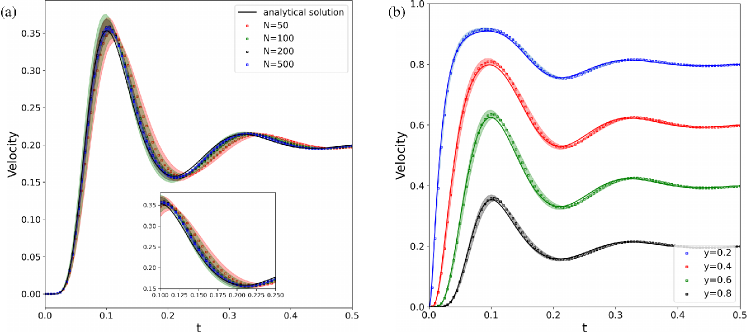
Figure 2: Time evolution of velocity at $y=0.8$ with different numbers of particles (a). Comparison of the velocity of the Hookean case (marker) with particle number $N=200$ and the analytical solution (continued line) with respect to time at different locations (b).

For the Oldroyd-B model, an analytical solution for the start-up of plane Couette flow in a 2D channel has been given, readers can refer to Refs. [40, 68]. We choose the physical parameters as follows: ${\rm Re}=0.11$, ${\rm Wi}=0.1$, $\tilde{\eta}_{s}=0.11$ and $\epsilon_{p}=0.89$. The number of elements is $M=40$ and the time step is $\Delta t=10^{-3}$. Additionally, we determine the kernel bandwidth using the formula $h_{p}=\mbox{med}^{2}/\log N$, where med is the median of the pairwise distance between the particles $\{\bm{q}_{i}^{n}\}_{i=1}^{N}$, following the approach outlined in Liu et al. [48].

We begin by examining the impact of the number of particles on numerical results. Figure 2(a) shows the time evolution of velocity at $y=0.8$ for different numbers of particles ($N=50,100,200,500$). Each marker on the plot represents the mean values of 10 independent runs, where we set the same parameters and used different sets of initial particles sampled from the standard normal distribution. While the shaded regions denote the standard errors of the 10 independent runs. The results indicate that as the number of particles increases, the standard deviations decrease, and the mean values will converge to the analytical solution. Figure 2 (b) presents the time evolution of the simulated velocity at $y=0.2,0.4,0.6,0.8$ for the micro-macro model with $N=200$ particles, compared to the analytical solution (continuous line). Since a good numerical result can be achieved with $N=200$, we set $N=200$ in all following numerical experiments.

4.2 FENE model: Hysteresis behavior in simple extensional flows

The FENE models account for the finite extensibility of polymer chains, and are able to capture the hysteresis behavior of dilute polymer solutions in simple extensional flow during relaxation, which can be observed through the normal stress or elongational viscosity versus mean-square extension [20, 42, 61]. However, many macroscopic closure models for the FENE potential fail to capture this behavior [31, 61]. In this subsection, we demonstrate that the deterministic particle scheme is capable of capturing the hysteresis behavior of a FENE model.

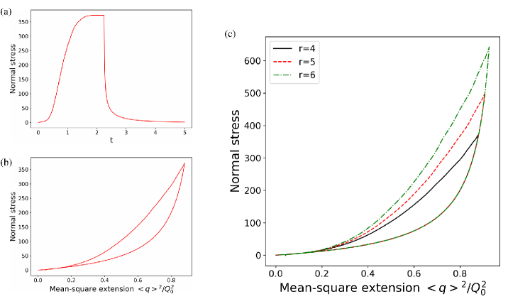
Figure 3: The start-up case with $r=4$: (a) the time evolution and (b) the hysteresis of normal stress $\tau_{11}-\tau_{22}$; (c) the hysteresis of the normal stress when $r=4$, $5$ and $6$.

We consider an elongational velocity gradient given by

$$\nabla\bm{u}=\varepsilon(t)\mbox{diag}(1,-1)\ ,$$ (35)

where $\varepsilon(t)$ is the strain rate and $\mbox{diag}(1,-1)$ is the 2 $\times$ 2 diagonal matrix with diagonal entries being $1$ and $-1$. Two cases of $\varepsilon(t)$ will be considered, the start-up case with

$$\varepsilon(t)=\left\{\begin{aligned} &r\qquad 0\leq t\leq\frac{9}{r}\ ,\\ &0\qquad\mbox{otherwise}\ ,\end{aligned}\right.$$ (36)

and the constant-gradient velocity case with

$$\varepsilon(t)=r\ .$$ (37)

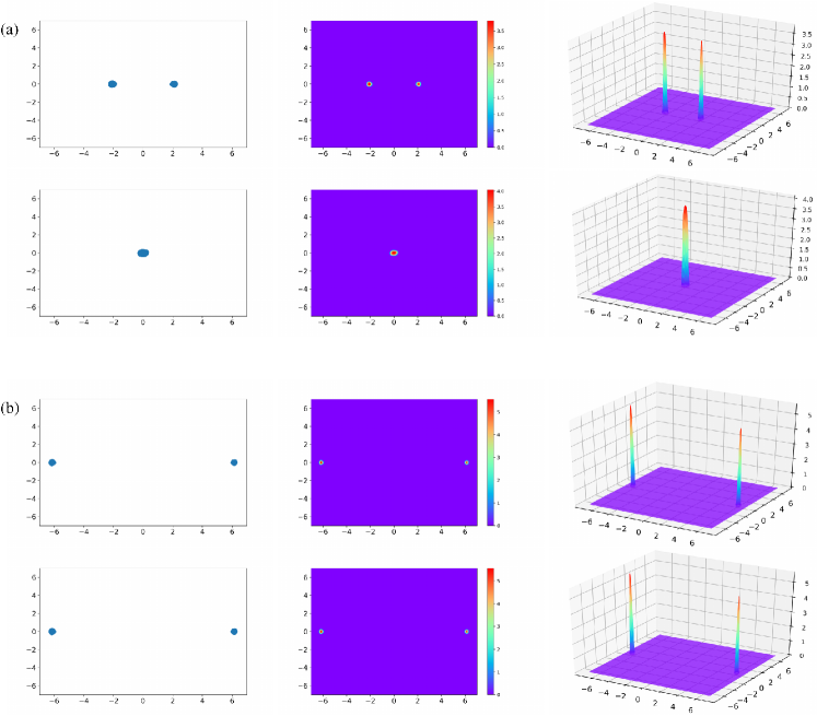
Figure 4: The particle and corresponding PDF (obtained by kernel density estimation) at different times. (a) Start-up case with $r=4$: the position of particles (left) and the distribution of particles (middle and right) at $t=3$ (the first row) and $t=8$ (the second row). (b) The constant-gradient velocity case with $r=4$: the position of particles (left) and the distribution of particles (middle and right) at $t=3$ (the first row) and $t=8$ (the second row).

Throughout this subsection, the initial data of particles is sampled from the 2-dimensional standard normal distribution. As stated in Section 4.1, we set $h_{p}=\mbox{med}^{2}/\log N$ for Hookean models, where med is the median of the pairwise distance between the particles $\{\bm{q}_{i}^{n}\}_{i=1}^{N}$. However, this approach is not suitable for the FENE potential, as the equilibrium distributions are no longer Gaussian type and the median of the pairwise distance can become very large. Numerical experiments show that taking $h_{p}=0.01$ produces a good result. Hence, for all the numerical experiments of the FENE case below, we set the kernel bandwidth $h_{p}=0.01$. Other parameters are set as follows, ${\rm Wi}=1;\ b=\sqrt{50};\ \Delta t=10^{-3}.$

For the start-up case, the time evolution of normal stress $\tau_{11}-\tau_{22}$ and the plot of the normal stress versus the mean-square extension $\langle\bm{q}^{2}\rangle/Q_{0}^{2}$ for $r=4$ are plotted in Figure 3 (a)-(b). The comparison of hysteresis behavior of the FENE model for different extensional rates ($r=4,5,6$) is shown in Figure 3 (c). It is observed that when the strength of velocity gradient is getting smaller, the hysteresis behavior becomes narrower. The numerical results are consistent with those obtained in the former work [31].

As discussed in [31], to catch the hysteresis of the original FENE model, a coarse grained model should be able to catch the spike like behaviors of the probability density in the FENE model in large extensional effect of the flow field. The peak positions of the probability distribution function (PDF) distribution of the FENE model depend on the macroscopic flow field and change in time under the large macroscopic flow effects [32]. We shows the distribution of the particles, and their underlying density (obtained by the kernel density estimation) at different times in the start-up case and the constant-gradient velocity case with $r=4$ in Figure 4. It reveals that the distribution of particles captures the $\delta$-function like spikes and the time evolution results of the particles apparently show a separation into two peaks in the two cases. In the start-up case, the distribution splits into two spikes and then shows gradual centralized behavior. Eventually, it forms a single peak in the center, as shown in Figure 4 (a). Notice that the numerical results in the equilibrium state are consistent with the equilibrium solution of the Fokker-Planck equation with zero flow rate. We can conclude that our numerical results are reasonable, since the velocity rate turns to be zero when $t$ is big enough ($t>9/r$). In the constant-gradient velocity case, the particles show two regions of higher concentration near the boundary of the configuration domain at the equilibrium state (i.e., with stable double spikes), as shown in Figure 4 (b). This is a good agreement to the feature of the FENE model.

4.3 FENE model: Simple shear flow

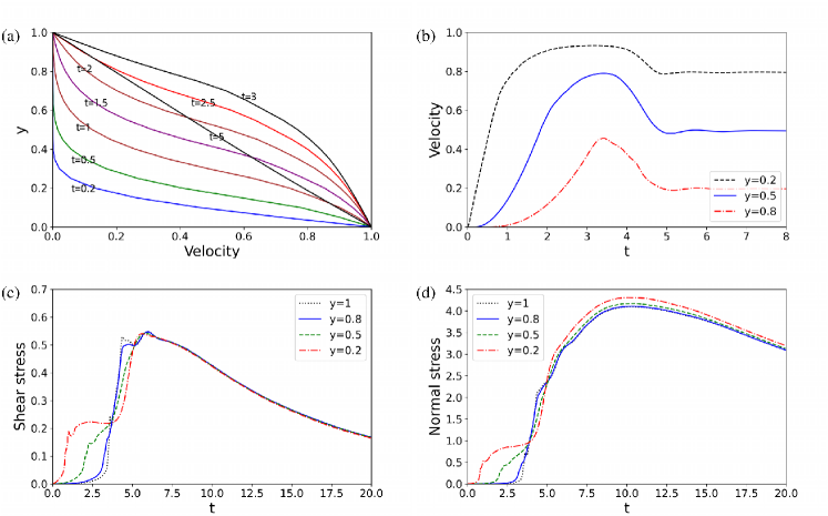
Figure 5: For the FENE model: the velocity $u$ with respect to location $y$ at different times (a); the time evolution of the velocity $u$ at different locations (b); the time evolution of the shear stress(c) and normal stress difference(d) at location $y=0.2$, $y=0.5$, $y=0.8$ and $y=1$.

In this subsection, we evaluate the proposed algorithm’s performance for the micro-macro model with a FENE potential in a start-up plane Couette flow as shown in Figure 1(a). We set $L=1$, $M=20$, $\Delta t=10^{-3}$. The non-dimensional parameters are chosen to be ${\rm Re}=1.2757$, $\tilde{\eta}_{s}=0.0521$, ${\rm Wi}=49.62$, $\epsilon_{p}=0.9479$, and $b=\sqrt{50}$, which are the same as those used in [40].

Figure 5 (a) shows the evolution of the velocity with respect to the location $y$ at different times. It reveals the velocity overshoot phenomenon for the FENE model, which is a typical property of viscoelastic fluids. Figure 5 (b) displays the evolution of the velocity with respect to time $t$ at three locations $y=0.2$, $y=0.5$ and $y=0.8$. It can be seen that the velocity overshoot occurs sooner in fluid layers nearer to the moving plane. Figures 5(c-d) show the temporal evolution of the shear stress and the normal stress difference at different locations $y=0.2$, $y=0.5$, $y=0.8$ and $y=1$. The stress response is sharper in fluid layers nearer to the moving plane, which is consistent with the behavior of velocity overshoot. We observe that the maximum of the normal stress occurs after the maximum of the shear stress. Specifically, the shear stress of the FENE model reaches its maximum at around $t=6$, but the maximum of the normal stress is reached at about $t=10$. The numerical results agree well with the former work [40, 68], indicating the accuracy of our numerical scheme in the FENE case. Moreover, compared with the former work, our numerical results obtained by the deterministic particle scheme show fewer oscillations.

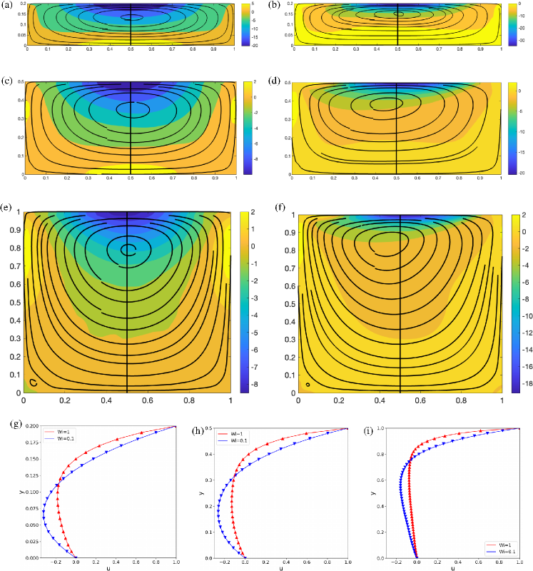
Figure 6: The streamlines and vortices contour of the lid driven cavity flow in the FENE case at $T=1$ with $L_{y}=0.2$ ((a): ${\rm Wi}=0.1$; (b): ${\rm Wi}=1$), $L_{y}=0.5$ ((c): ${\rm Wi}=0.1$; (d): ${\rm Wi}=1$) and $L_{y}=1$ ((e): ${\rm Wi}=0.1$; (f): ${\rm Wi}=1$). The profile of $u$-velocity with respect to $y$ at position $x=0.5$ for ${\rm Wi}=0.1,1$ with $L_{y}=0.2$ (left), $L_{y}=0.5$ (middle) and $L_{y}=1$ (right).

4.4 FENE model: Lid driven cavity flow

In this subsection, we simulate the FENE model for lid-driven cavity flows (see Figure 1(b)). It is a 2D problem and a full 2D Navier-Stokes equation needs to be solved. Our experiments consider rectangular cavities with different heights: $L_{y}=0.2$, $0.5$, and $1$. In order to avoid numerical difficulties that arise from the geometric singularity at the edges of an idealized lid-driven cavity, we adopt a regularized horizontal lid velocity [62] of the form:

$$u(x)=16U(x/L_{x})^{2}(1-x/L_{x})^{2}.$$

To discretize the problem spatially, we choose $\mathcal{T}_{h}$ to be a uniform triangular mesh with the mesh size $N_{x}=50,N_{y}=20$ for $L_{y}=0.2$, $N_{x}=50,N_{y}=25$ for $L_{y}=0.5$, and $N_{x}=50,N_{y}=50$ for $L_{y}=1$. We set the time step size $\Delta t=10^{-3}$ for temporal discretization. Unlike the shear flow cases, the convection term $\bm{u}\cdot\nabla\bm{q}$ is non-zero, which is dealt with by a Lagrangian approach as introduced in Section 3. Other parameters in the numerical experiments are set as follows: ${\rm Re}=1;\ \tilde{\eta}_{s}=0.11;\ \epsilon_{p}=0.889;\ b=\sqrt{50}.$

Figure 6(a)-(f) display the streamlines and vortices contours for different $L_{y}$ at time $T=1$ with ${\rm Wi}=0.1$ and ${\rm Wi}=1$. Notice that the streamlines show symmetry structure when ${\rm Wi}=0.1$. And this symmetry structure holds for different $L_{y}$. However, as elasticity becomes more important, namely, the Weissenberg number (${\rm Wi}$) increases, the symmetries in the streamline structures break due to the presence of elastic effects [17]. Meanwhile, as the flow becomes asymmetric, the vortex center in the cavity shifts progressively upward and opposite to the direction of lid motion [26]. This phenomenon is more evident in Figure 6(g)-(i), which plot the $u$-velocity profiles at $x=0.5$ for the cavity flow with different $L_{y}$ and ${\rm Wi}$. Additionally, the introduction of elasticity also weakens the strengths of vortices near the moving lid [62]. The numerical results indicate that the particle-based scheme can capture these complex behaviors. The qualitative agreement between our simulation results and those of the former work [26, 68] validates our numerical scheme for the 2D lid-driven cavity flow case.

5 Conclusion

In this article, we present a novel deterministic particle-finite element method (FEM) discretization for micro-macro models of dilute polymeric fluids. The proposed scheme employs a coupled numerical solution for the macro- and microscopic scales, with the finite element method used for the fluid flow equation and the variational particle scheme used for the kinetic viscoelastic model. The coarse-grained model of particles is derived via a discrete energy variational approach, which preserves the variational structure at the particle level. The proposed scheme is validated through various benchmark problems, including steady flow, shear flow and 2D lid-driven cavity flow. Our numerical results are in excellent agreement with those from the former work and demonstrate that the proposed scheme is able to capture certain complex behaviors of the nonlinear FENE model, including the hysteresis and $\delta$-function like spike behavior in extension flows, velocity overshoot phenomenon in pure shear flow, symmetries breaking, vortex center shifting and vortices weakening in lid-driven cavity flow. Moreover, our numerical results obtained by the deterministic particle scheme are shown to have fewer oscillations and to be be more efficient than the stochastic approach in the former work, where a large ensemble of realizations of the stochastic process are needed.

The proposed method can also be applied to other complex fluid models, such as the Doi-Onsager model for liquid crystal polymers [19], the multi-bead spring model [69], and a two-species model for wormlike micellar solutions [47, 67], which involves a reaction in the microscopic equation. Additionally, as a direction for future work, we aim to develop an energy-stable scheme for the overall system.

References

- Ammar [2010] Ammar, A., 2010. Lattice Boltzmann method for polymer kinetic theory. J. Non-Newtonian Fluid Mech. 165, 1082–1092.
- Arnold [2013] Arnold, V., 2013. Mathematical methods of classical mechanics. Graduate Texts in Mathematics, 60. Springer-Verlag, New York.
- Arroyo and Ortiz [2006] Arroyo, M., Ortiz, M., 2006. Local maximum-entropy approximation schemes: a seamless bridge between finite elements and meshfree methods. Int. J. Numer. Meth. Engng. 65, 2167–2202.
- Bao et al. [2021] Bao, X., Chen, R., Zhang, H., 2021. Constraint-preserving energy-stable scheme for the 2d simplified ericksen-leslie system. J. Comput. Math. 39, 1–21.
- Becker et al. [2008] Becker, R., Feng, X., Prohl, A., 2008. Finite element approximations of the ericksen-leslie model for nematic liquid crystal flow. SIAM J. Numer. Anal. 46, 1704–1731.
- Bergamasco et al. [2013] Bergamasco, L., Izquierdo, S., Ammarb, A., 2013. Direct numerical simulation of complex viscoelastic flows via fast lattice-Boltzmann solution of the Fokker-Planck equation. J. Non-Newtonian Fluid Mech. 201, 29–38.
- Bird et al. [1987] Bird, R., Curtiss, C., Armstrong, R., Hassager, O., 1987. Dynamics of Polymeric Liquids, Kinetic Theory (Dynamics of Polymer Liquids, vol. 1 and 2). Wiley-Interscience, New York.
- Bird and Öttinger [1992] Bird, R., Öttinger, H., 1992. Transport properties of polymeric liquids. Annu. Rev. Phys. Chem. 43, 371–406.
- Boffi et al. [2013] Boffi, D., Brezzi, F., Fortin, M., 2013. Mixed Finite Element Methods and Applications. Springer Series in Computational Mathematics, 44, Springer, Heidelberg.
- Boyaval and Lelièvre [2010] Boyaval, S., Lelièvre, T., 2010. A variance reduction method for parametrized stochastic differential equations using the reduced basis paradigm. Commun. Math. Sci. 8, 735–762.
- Brezzi and Fortin [1991] Brezzi, F., Fortin, M., 1991. Mixed and Hybrid Finite Element Methods. Springer-Verlag.
- Bris and Lelièvre [2012] Bris, C.L., Lelièvre, T., 2012. Micro-macro models for viscoelastic fluids: modelling, mathematics and numerics. Sci. China Math. 55, 353–384.
- Carrillo et al. [2019] Carrillo, J.A., Craig, K., Patacchini, F.S., 2019. A blob method for diffusion. Calc. Var. 58, 53.
- Chauviere [2002] Chauviere, C., 2002. A new method for micro-macro simulations of viscoelastic flows. SIAM J. Sci. Comput. 23, 2123–2140.
- Chauvière and Lozinski [2004] Chauvière, C., Lozinski, A., 2004. Simulation of dilute polymer solutions using a Fokker-Planck equation. Comput. Fluids 33, 687–696.
- Chen et al. [2015] Chen, R., Ji, G., Yang, X., Zhang, H., 2015. Decoupled energy stable schemes for phase-field vesicle membrane model. J. Comput. Phys. 302, 509–523.
- Dalal et al. [2016] Dalal, S., Tomar, G., Dutta, P., 2016. Numerical study of driven flows of shear thinning viscoelastic fluids in rectangular cavities. J. Non-Newtonian Fluid Mech. 229, 59–78.
- Degond and Mustieles [1990] Degond, P., Mustieles, F.J., 1990. A deterministic approximation of diffusion equations using particles. SIAM J. Sci. Statist. Comput. 11, 293–310.
- Doi and Edwards [1988] Doi, M., Edwards, S.F., 1988. The theory of polymer dynamics. volume 73. oxford university press.
- Doyle et al. [1998] Doyle, P.S., Shaqfeh, E.S., McKinley, G.H., Spiegelberg, S.H., 1998. Relaxation of dilute polymer solutions following extensional flow. J. Non-Newtonian Fluid Mech. 76, 79–110.
- Du et al. [2005] Du, Q., Liu, C., Yu, P., 2005. FENE dumbbell model and its several linear and nonlinear closure approximations. Multiscale Model. Simul. 4, 709–731.
- E et al. [2009] E, W., Ren, W., Vanden-Eijnden, E., 2009. A general strategy for designing seamless multiscale methods. J. Comput. Phys. 228, 5437–5453.
- Ericksen [1992] Ericksen, J.L., 1992. Reversible and nondissipative processes. Quart. J. Mech. Appl. Math. 45, 545–554.
- Giga et al. [2017] Giga, M., Kirshtein, A., Liu, C., 2017. Variational modeling and complex fluids. Handbook of mathematical analysis in mechanics of viscous fluids , 1–41.
- Griebel and Rüttgers [2014] Griebel, M., Rüttgers, A., 2014. Multiscale simulations of three-dimensional viscoelastic flows in a square–square contraction. J. Non-Newtonian Fluid Mech. 205, 42–63.
- Grillet et al. [1999] Grillet, A., Yang, B., Khomami, B., Shaqfeh, E., 1999. Modeling of viscoelastic lid driven cavity flow using finite element simulations. J. Non-Newtonian Fluid Mech. 88, 99–131.
- Guermond et al. [2006] Guermond, J.L., Minev, P., Shen, J., 2006. An overview of projection methods for incompressible flows. Comput. Methods Appl. Mech. Engrg. 195, 6011–6045.
- Halin et al. [1998] Halin, P., Lielens, G., Keunings, R., Legat, V., 1998. The Lagrangian particle method for macroscopic and micro-macro viscoelastic flow computations. J. Non-Newtonian Fluid Mech. 79, 387–403.
- Helzel and Otto [2006] Helzel, C., Otto, F., 2006. Multiscale simulations for suspensions of rod-like molecules. J. Comput. Phys. 216, 52–75.
- Hulsen et al. [1997] Hulsen, M., van Heel, A., van den Brule, B., 1997. Simulation of viscoelastic flows using Brownian configuration fields. J. Non-Newtonian Fluid Mech. 70, 79–101.
- Hyon [2014] Hyon, Y., 2014. Hysteretic behavior of a moment-closure approximation for fene model. Kinet. Relat. Mod. 7, 493–507.
- Hyon et al. [2008] Hyon, Y., Du, Q., Liu, C., 2008. An enhanced macroscopic closure approximation to the micro-macro fene model for polymeric materials. Multiscale Model. Simul. 7, 978–1002.
- Jourdain et al. [2004] Jourdain, B., Bris, C.L., Lelièvre, T., 2004. On a variance reduction technique for micro-macro simulations of polymeric fluids. J. Non-Newtonian Fluid Mech. 122, 91–106.
- Jourdain et al. [2002] Jourdain, B., Lelièvre, T., Bris, C.L., 2002. Numerical analysis of micro-macro simulations of polymeric fluid flows: a simple case. Math. Mod. Meth. Appl. S. 12, 1205–1243.
- Keunings [1997] Keunings, R., 1997. On the peterlin approximation for finitely extensible dumbbells. J. Non-Newtonian Fluid Mech. 68, 85–100.
- Knezevic and Süli [2009] Knezevic, D., Süli, E., 2009. A heterogeneous alternating-direction method for a micro-macro dilute polymeric fluid model. M2AN Math. Model. Numer. Anal. 43, 1117–1156.
- Koppol et al. [2007] Koppol, A.P., Sureshkumar, R., Khomami, B., 2007. An efficient algorithm for multiscale flow simulation of dilute polymeric solutions using bead-spring chains. J. Non-Newtonian Fluid Mech. 141, 180–192.
- Lacombe and Mas-Gallic [1999] Lacombe, G., Mas-Gallic, S., 1999. Presentation and analysis of a diffusion-velocity method, in: ESAIM: Proc., EDP Sciences. pp. 225–233.
- Larson [1998] Larson, R., 1998. The Structure and Rheology of Complex Fluids. Oxford University Press, Oxford.
- Laso and Öttinger [1993] Laso, M., Öttinger, H., 1993. Calculation of viscoelastic flow using molecular models: The CONNFFESSIT approach. J. Non-Newtonian Fluid Mech. 47, 1–20.
- Li and Zhang [2007] Li, T., Zhang, P., 2007. Mathematical analysis of multi-scale models of complex fluids. Commun. Math. Sci. 5, 1–51.
- Lielens et al. [1998] Lielens, G., Halin, P., Jaumain, I., Keunings, R., Legat, V., 1998. New closure approximations for the kinetic theory of finitely extensible dumbbells. J. Non-Newtonian Fluid Mech. 76, 249–279.
- Lin [2012] Lin, F., 2012. Some analytical issues for elastic complex fluids. Comm. Pure Appl. Math. 65, 893–919.
- Lin et al. [2007] Lin, F., Liu, C., Zhang, P., 2007. On a micro-macro model for polymeric fluids near equilibrium. Comm. Pure Appl. Math. 60, 838–866.
- Liu [2009] Liu, C., 2009. An introduction of elastic complex fluids: an energetic variational approach, in: Multi-Scale Phenomena in Complex Fluids: Modeling, Analysis and Numerical Simulation. World Scientific, pp. 286–337.
- Liu and Wang [2020] Liu, C., Wang, Y., 2020. On Lagrangian schemes for porous medium type generalized diffusion equations: A discrete energetic variational approach. J. Comput. Phys. 417, 109566.
- Liu et al. [2022] Liu, C., Wang, Y., Zhang, T.F., 2022. Global existence of classical solutions for a reactive polymeric fluid near equilibrium. Calc. Var. Partial Differential Equations 61, Paper No. 117, 37 pp.
- Liu and Wang [2016] Liu, Q., Wang, D., 2016. Stein variational gradient descent: A general purpose bayesian inference algorithm. Adv. Neural Inf. Process. Syst. 29.
- Lozinski and Chauvière [2003] Lozinski, A., Chauvière, C., 2003. A fast solver for Fokker-Planck equation applied to viscoelastic flows calculations: 2D FENE model. J. Comput. Phys. 189, 607–625.
- Lozinski et al. [2011] Lozinski, A., Owens, R.G., Phillips, T.N., 2011. The Langevin and Fokker–Planck equations in polymer rheology. Handbook of Numerical Analysis 16, 211–303.
- Oldroyd [1950] Oldroyd, J., 1950. On the formulation of rheological equations of state. Proc. R. Soc. Lond. A 200, 523–541.
- Onsager [1931a] Onsager, L., 1931a. Reciprocal relations in irreversible processes. I. Phys. Rev. 37, 405.
- Onsager [1931b] Onsager, L., 1931b. Reciprocal relations in irreversible processes. II. Phys. Rev. 38, 2265.
- Öttinger [1996] Öttinger, H., 1996. Stochastic Processes in Polymeric Fluids, Tools and Examples for Developing Simulation Algorithms. Springer-Verlag, Berlin.
- Öttinger et al. [1997] Öttinger, H., Brule, B.V.D., Hulsen, M., 1997. Brownian configuration fields and variance reduced connffessit. J. Non-Newtonian Fluid Mech. 70, 255–261.
- Peterlin [1966] Peterlin, A., 1966. Hydrodynamics of macromolecules in a velocity field with longitudinal gradient. J. Polymer Sci., B 4, 287–291.
- Rayleigh [1871] Rayleigh, L., 1871. Some general theorems relating to vibrations. Proc. Lond. Math. Soc. 1, 357–368.
- Rosolen et al. [2013] Rosolen, A., Peco, C., Arroyo, M., 2013. An adaptive meshfree method for phase-field models of biomembranes. part i: Approximation with maximum-entropy basis functions. J. Comput. Phys. 249, 303–319.
- Russo [1990] Russo, G., 1990. Deterministic diffusion of particles. Comm. Pure Appl. Math. 43, 697–733.
- Shen and Yu [2012] Shen, J., Yu, H., 2012. On the approximation of the Fokker–Planck equation of the finitely extensible nonlinear elastic dumbbell model I: A new weighted formulation and an optimal spectral-Galerkin algorithm in two dimensions. SIAM J. Numer. Anal. 50, 1136–1161.
- Sizaire et al. [1999] Sizaire, R., Lielens, G., Jaumain, I., Keunings, R., Legat, V., 1999. On the hysteretic behaviour of dilute polymer solutions in relaxation following extensional flow. J. Non-Newtonian Fluid Mech. 82, 233–253.
- Sousa et al. [2016] Sousa, R., Poole, R., Afonso, A., Pinho, F., Oliveira, P., Morozov, A., Alves, M., 2016. Lid-driven cavity flow of viscoelastic liquids. J. Non-Newtonian Fluid Mech. 234, 129–138.
- Suen et al. [2002] Suen, J., Joo, Y.L., Armstrong, R., 2002. Molecular orientation effects in viscoelasticity. Annu. Rev. Fluid Mech. 34, 417–444.
- Tabata and Tagami [2000] Tabata, M., Tagami, D., 2000. Error estimates for finite element approximations of drag and lift in nonstationary navier-stokes flows. Jpn. J. Ind. Appl. Math. 17, 371–389.
- Wang et al. [2021a] Wang, Y., Chen, J., Kang, L., Liu, C., 2021a. Particle-based energetic variational inference. Stat. Comput. 31, Paper No. 34, 17pp.
- Wang et al. [2020] Wang, Y., Liu, C., Liu, P., Eisenberg, B., 2020. Field theory of reaction-diffusion: law of mass action with an energetic variational approach. Phys. Rev. E 102, 062147, 9 pp.
- Wang et al. [2021b] Wang, Y., Zhang, T.F., Liu, C., 2021b. A two species micro–macro model of wormlike micellar solutions and its maximum entropy closure approximations: An energetic variational approach. J. Non-Newtonian Fluid Mech. 293, 104559.
- Xu et al. [2014] Xu, X., Ouyang, J., Li, W., Liu, Q., 2014. SPH simulations of 2D transient viscoelastic flows using Brownian configuration fields. J. Non-Newtonian Fluid Mech. 208-209, 59–71.
- Zhou and Akhavan [2004] Zhou, Q., Akhavan, R., 2004. Cost-effective multi-mode fene bead-spring models for dilute polymer solutions. J. Non-Newtonian Fluid Mech. 116, 269–300.