On the Size and Width of the Decoder of a Boolean Threshold Autoencoder

Abstract

In this paper, we study the size and width of autoencoders consisting of Boolean threshold functions, where an autoencoder is a layered neural network whose structure can be viewed as consisting of an encoder, which compresses an input vector to a lower dimensional vector, and a decoder which transforms the low-dimensional vector back to the original input vector exactly (or approximately). We focus on the decoder part, and show that $\Omega(\sqrt{Dn/d})$ and $O(\sqrt{Dn})$ nodes are required to transform $n$ vectors in $d$-dimensional binary space to $D$-dimensional binary space. We also show that the width can be reduced if we allow small errors, where the error is defined as the average of the Hamming distance between each vector input to the encoder part and the resulting vector output by the decoder.

Keywords: Neural networks, Boolean functions, threshold functions, autoencoders.

1 Introduction

Extensive studies have been done on artificial neural networks not only in artificial intelligence and machine learning but also in theoretical computer science [2, 12, 10]. Among various models of neural networks, autoencoders have recently attracted much attention due to their ability to generate new data, and have been applied to various areas including image processing [5, 11], natural language processing [11], and drug discovery [6]. An autoencoder is a layered neural network consisting of two parts, an encoder and a decoder, where the former transforms an input vector to a low-dimensional vector and the latter transforms the low-dimensional vector to an output vector which should be the same as or similar to the input vector [1, 4, 7, 3]. Therefore, an autoencoder maps input data to a low-dimensional representation space. Such a mapping is obtained via unsupervised learning that minimizes the difference between input and output data by adjusting weights (and some other parameters).

Although autoencoders perform dimensionality reduction, a kind of data compression, how data are compressed via autoencoders is still unclear. In particular, the quantitative relationship between the compressive power and the numbers of nodes and layers in autoencoders had been unclear. In order to study the relationship, Melkman et al. analyzed the relations between the architecture (e.g., the numbers of nodes and layers) of networks and their compression ratios [8], using a layered Boolean threshold network, which is a discrete model of neural networks. A Boolean threshold network is equivalent to a threshold circuit [2, 12, 10] in which each node takes on values that are either 1 (active) or 0 (inactive) and the activation rule for each node is given by a Boolean threshold function. In [8] several architectures of autoencoders were presented that map $n$ $D$-dimensional binary input vectors into $d$-dimensional binary space and then recover the original input vectors. In particular, they showed the following architectures for $d=\lceil\log n\rceil$ (or, almost equivalently, $d=2\lceil\log\sqrt{n}\rceil$):

• a 4-layers encoder with $O(\sqrt{n}+D)$ nodes;

• a 5-layers autoencoder with $D/n/d/n/D$ architecture, where each parameter means the number of nodes in the corresponding layer;

• a 7-layers autoencoder with $O(D\sqrt{n})$ nodes;

• a decoder with depth $n+1$ and width $O(D)$, where the width is the maximum number of nodes per layer (except for the input and output layers) and the depth is the number of layers minus one.

However, it was unclear whether or not these results are optimal (or near optimal).

In this paper, we focus on the decoder part because the decoders (in the above-quoted results) use $O(D\sqrt{n})$, $O(n+D)$, or more nodes whereas the encoder uses only $O(\sqrt{n}+D)$ nodes. We show an $\Omega(\sqrt{Dn/d})$ lower bound on the size of the perfect decoder, where a decoder is called perfect if it can always recover the original input vectors exactly. To our knowledge, this is the first lower bound result on the size (i.e., the number of nodes) of the autoencoder. As a positive result, we show that there exists a perfect decoder with width $\max(\lceil n/B\rceil+B,BD)$ and a constant depth, where $B$ is an arbitrary integer larger than 1. By letting $B=\lceil\sqrt{n/D}\rceil$, we obtain an $O(\sqrt{Dn})$ upper bound on the size and width of the decoder, which is relatively close to the lower bound and improves the previous $O(D\sqrt{n})$ upper bound. In order to construct decoders that have even smaller width we permit them to output vectors that are in error, where the error is defined as the average of the Hamming distance between each vector input to the encoder part and the resulting vector output by the decoder. We show that there exists a decoder with width $\max(\lceil n/B\rceil+B,(B-1)D+1)$ and a constant depth whose error is at most $D({\frac{1}{B2^{B}}}+{\frac{1}{n}})$.

2 Preliminaries

A function $f$: $\{0,1\}^{h}\rightarrow\{0,1\}$ is called a Boolean threshold function if it is represented as

$$f({\bf x})=\left\{\begin{array}[]{ll}1,&{\bf a}\cdot{\bf x}\geq\theta,\\ 0,&\mbox{otherwise,}\end{array}\right.$$

for some $({\bf a},\theta)$, where ${\bf a}$ is an $h$-dimensional integer vector and $\theta$ is an integer. We will also denote the same function as $[{\bf a}\cdot{\bf x}\geq\theta]$. An acyclic network is called a Boolean threshold network (BTN) if all activation functions in the network are Boolean threshold functions.

In this paper, we only consider layered BTNs in which nodes are divided into $L$-layers and each node in the $i$-th layer has inputs only from nodes in the ($i-1$)th layer ($i=1,\ldots,L-1$). Then, the states of nodes in the $i$-th layer can be represented as a $W_{i}$-dimensional binary vector where $W_{i}$ is the number of nodes in the $i$-th layer and is called the width of the layer. A layered BTN is represented as ${\bf y}={\bf f}^{(L-1)}({\bf f}^{(L-2)}(\cdots{\bf f}^{(1)}({\bf x})\cdots))$, where ${\bf x}$ and ${\bf y}$ are the input and output vectors, respectively. and ${\bf f}^{(i)}$ is a list of activation functions for the ($i+1$)th layer. The $0$-th and ($L-1$)-th layers are called the input and output layers, respectively, and the corresponding nodes are called input and output nodes, respectively. The size, depth, width of a layered BTN are defined as the number of nodes, the number of layers minus one, and the maximum number of nodes in a layer (excepting the input and output layers), respectively. When we consider autoencoders, one layer ($k$-th layer where $k\in\{1,\ldots,L-2\}$) is specified as the middle layer, and the nodes in this layer are called the middle nodes (see also Fig. 1). Then, the middle vector ${\bf z}$, encoder ${\bf f}$, and decoder ${\bf g}$ are defined by

$${\bf z} = {\bf f}^{(k-1)}({\bf f}^{(k-2)}(\cdots{\bf f}^{(1)}({\bf x})\cdots))={\bf f}({\bf x}),$$

$${\bf y} = {\bf f}^{(L-1)}({\bf f}^{(L-2)}(\cdots{\bf f}^{(k)}({\bf z})\cdots))={\bf g}({\bf z}).$$

Since the input vectors should be recovered from the middle vectors at the output layer, we assume that ${\bf x}$ and ${\bf y}$ are $D$-dimensional binary vectors and ${\bf z}$ is a $d$-dimensional binary vector with $d\leq D$. A list of functions is also referred to as a mapping. The $i$-th element of a vector ${\bf x}$ will be denoted by $x_{i}$, which is also used to denote the node corresponding to this element. Similarly, for each mapping ${\bf f}$, $f_{i}$ denotes the $i$-th function.

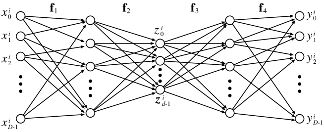
Figure 1: Architecture of a five-layer autoencoder, where ${\bf z}={\bf f}({\bf x})={\bf f}_{2}({\bf f}_{1}({\bf x}))$ and ${\bf y}={\bf g}({\bf z})={\bf f}_{4}({\bf f}_{3}({\bf z}))$.

Let $X_{n}=\{{\bf x}^{0},\ldots,{\bf x}^{n-1}\}$ be a set of $n$ $D$-dimensional binary input vectors that are all different. We define perfect encoder, decoder, autoencoder as follows [8].

Definition 1.

A mapping ${\bf f}$: $\{0,1\}^{D}\rightarrow\{0,1\}^{d}$ is called a perfect encoder for $X_{n}$ if ${\bf f}({\bf x}^{i})\neq$ ${\bf f}({\bf x}^{j})$ holds for all $i\neq j$.

Definition 2.

A pair of mappings $({\bf f},{\bf g})$ with ${\bf f}$: $\{0,1\}^{D}\rightarrow\{0,1\}^{d}$ and ${\bf g}$: $\{0,1\}^{d}\rightarrow\{0,1\}^{D}$ is called a perfect autoencoder if ${\bf g}({\bf f}({\bf x}^{i}))={\bf x}^{i}$ holds for all ${\bf x}^{i}\in X_{n}$. Furthermore, such ${\bf g}$ is called a perfect decoder.

Note that a perfect decoder exists only if there exists a perfect autoencoder. Furthermore, it is easily seen from the definitions that if $({\bf f},{\bf g})$ is a perfect autoencoder, ${\bf f}$ is a perfect encoder.

Example 3.

Let $X_{4}=\{{\bf x}^{0},{\bf x}^{1},{\bf x}^{2},{\bf x}^{3}\}$ where ${\bf x}^{0}=(0,0,0)$, ${\bf x}^{1}=(1,0,0)$, ${\bf x}^{2}=(1,0,1)$, ${\bf x}^{3}=(1,1,1)$. Let $D=3$ and $d=2$. Define ${\bf z}={\bf f}({\bf x})$ and ${\bf y}={\bf g}({\bf z})$ by

$$f_{0}({\bf x}) = [x_{0}+x_{1}-x_{2}\geq 1],~{}~{}~{}f_{1}({\bf x})~{}=~{}[x_{2}\geq 1],$$

$$g_{0}({\bf z}) = [z_{0}+z_{1}\geq 1],~{}~{}~{}g_{1}({\bf z})~{}=~{}[z_{0}+z_{1}\geq 2],~{}~{}~{}g_{2}({\bf z})~{}=~{}[z_{1}\geq 1].$$

This pair of mappings has the following truth table, which shows it to be a perfect autoencoder.

$x_{0}$	$x_{1}$	$x_{2}$	$z_{0}$	$z_{1}$	$y_{0}$	$y_{1}$	$y_{2}$
0	0	0	0	0	0	0	0
1	0	0	1	0	1	0	0
1	0	1	0	1	1	0	1
1	1	1	1	1	1	1	1

3 A Lower Bound on the Size of the Decoder

In this section we derive a lower bound on the number of threshold units (i.e., the number of nodes except those in the input layer) in the decoder BTN of a Boolean threshold autoencoder which perfectly encodes every possible set of $n$ $D$-dimensional vectors, and which has a middle layer whose size is less than one third the size of the output layer. Note that $n\leq 2^{d}$, since $n$ vectors are perfectly encoded.

Denote the number of threshold units of the decoder-BTN by $N$, with the $i$-th unit having $d_{i}$ inputs, where $N$ includes the number of output nodes but does not include the number of middle nodes.

Theorem 4.

There exists a set $X_{n}$ for which there is no perfect autoencoder with a middle layer of size $d$ and a decoder of size less than $\sqrt{\frac{D-1}{3d}}\sqrt{n}$.

Proof.

The idea is to calculate an upper bound on the total number of different sets of $n$ vectors that can be generated at the output layer of the autoencoder from all possible sets of $d$-dimensional vectors, input to the middle layer, by all possible different decoder BTNs. Let’s denote that number $PD$ (the in-Principle Decoded sets). Since the autoencoder is perfect, $PD$ is not smaller than the number of different sets of $D$-dimensional output (=input) vectors of the autoencoder, each of size $n$, which is $\binom{2^{D}}{n}$.

Next we derive an upper bound on $PD$. Each threshold unit computes a Boolean function of the $d$ inputs (in the middle-layer). In the course of proving Theorem 7.4 of [2], which provides a lower bound on the size of the universal networks, it is shown that the number of different functions representable by a threshold unit with in-degree $d_{i}$ in an acyclic BTN which has $d$ input nodes is at most $2^{dd_{i}+1}$. Therefore, an upper bound on the total number of functions from $\{0,1\}^{d}$ to $\{0,1\}^{D}$ computable by a decoder BTN with $N$ nodes is

$$\prod_{i=1}^{N}2^{dd_{i}+1}=2^{N+d\sum_{i=0}^{N-1}d_{i}}\leq 2^{N+dN^{2}}.$$

Since the number of all possible ordered sets of $n$ $d$-dimensional vectors in the middle layer does not exceed $2^{d}!/(2^{d}-n)!\leq(2^{d})^{n}$ we conclude that

$${\frac{(2^{D}-n)^{n}}{n^{n}}}\leq\binom{2^{D}}{n}\leq PD\leq\left[(2^{d})^{n}\right]\cdot\left[2^{N+dN^{2}}\right]$$

Taking base 2 logarithms of both sides shows that the parameters of the decoder satisfy $nd+N+dN^{2}\geq n\log(2^{D}-n)-n\log n$. Noting that $n\leq 2^{d}<2^{D-1}$ yields $N+dN^{2}>n(D-1)-2nd$. Applying the precondition $d\leq{\frac{D-1}{3}}$ results in the inequality

$$N+dN^{2}>{\frac{n}{3}}(D-1),$$

from which the theorem follows. ∎

Remarks:

• This lower bound is meaningful only if $\sqrt{\frac{D-1}{3d}}\sqrt{n}\geq D$ because the decoder contains $D$ output nodes.

• In the proof $d_{i}$ was replaced by its upper bound $N$. Therefore, the lower bound stated in the Theorem holds for any acyclic decoder.

• The stated lower bound becomes an $\Omega(\sqrt{Dn/d})$ lower bound on the widths of layered BTN decoders of constant depth.

4 Decoder with Width $\max(\lceil n/B\rceil+B,BD)$

In this section we present the architecture of a decoder BTN that is able to decode perfectly any set of $n$ $D$-dimensional vectors that has been encoded into a layer of size $d$ (so that the encoder and decoder together perfectly autoencode every such set), where $d=\lceil\log n\rceil$.

We will use $\beta_{0},\ldots,\beta_{d-1}$ to refer to the middle nodes as well as to their values, with $\beta$ denoting the vector $(\beta_{0},\ldots,\beta_{d-1})$. $Int(\beta)$ denotes the integer encoded by $\beta$, i.e. $Int(\beta)=\sum_{i=0}^{d-1}\beta_{i}2^{d-i-1}$.

Let $B$ be an integer greater than 1. For ease of exposition we assume that $n$ can be divided by $B$ and use $n_{B}$ to denote $n/B$. Otherwise we can let $n_{B}=\lceil n/B\rceil$. In this section we detail the architecture of a $d/{\frac{n}{B}}+B/BD/D$ decoder (with $B=2^{K}$ for some integer $K$), see Figure 2. In addition to $\beta$ it has the following nodes:

• $\gamma_{0},\gamma_{1},\ldots,\gamma_{n_{B}-1},\gamma_{n_{B}},\gamma_{n_{B}+1},\ldots,\gamma_{n_{B}+B-1}$,

• $y_{j,b}$ for $j=0,\ldots,D-1$ and $b=0,\ldots,B-1$,

• $y_{j}$ for $j=0,\ldots,D-1$, the output nodes.

The activation function of the $\gamma_{i}$ are:

$$\gamma_{i} = [\lfloor{\frac{Int(\beta)}{B}}\rfloor=i],~{}~{}~{}\mbox{for $i=0,\ldots,n_{B}-1$},$$

$$\gamma_{n_{B}+h} = [Int(\beta)=h~{}(\mbox{mod $B$})],~{}~{}~{}\mbox{for $h=0,\ldots,B-1$},$$

where $[Int(\beta)=k]$ takes value 1 if $Int(\beta)=k$, and value 0 otherwise. Note that division and modulo operations can be done by threshold circuits of width $O(poly(\log n))$ and depth 5 [9] (recall that $\beta$ is a vector of dimension $O(\log n)$), a negligible increase to the $O(\sqrt{Dn})$ width of our network. Furthermore, if $B=2^{K}$ for some integer $K$, we do not need such circuits because we can simply use the first $d-K$ bits of $\beta$ to represent $Int(\beta)/B$ and the remaining $K$ bits to represent $Int(\beta)\mbox{ mod $B$}$. Note also that $[Int(\beta)=k]$ can be calculated by using a single unit with an activation function ${\bf a}\cdot\beta\geq\theta$ such that

$$a_{i} = \left\{\begin{array}[]{ll}1,&\mbox{if $k_{i}=1$},\\ -1,&\mbox{otherwise},\end{array}\right.$$

$$\theta = \sum_{i}k_{i},$$

where $k_{0}k_{1}\cdots k_{d-1}$ is the binary representation of an integer $k$.

The activation function of $y_{j,b}$ is

$$y_{j,b}=[\sum_{i=0}^{n_{B}+B-1}w_{i,j,b}\gamma_{i}\geq 2],$$

where $w_{i,j,b}$ is given by

$$w_{h,j,b} = x_{j}^{Bh+b}~{}~{}~{}\mbox{for $h=0,\ldots,n_{B}-1$ and for $b=0,\ldots,B-1$},$$

$$w_{n_{B}+h,j,b} = [h=b]~{}~{}~{}\mbox{for $h=0,\ldots,B-1$ and for $b=0,\ldots,B-1$}.$$

Numbering the $n$ input/output vectors so that each ${\bf x}^{k}$ is mapped to $\beta$ with $Int(\beta)=k$, it is not difficult to verify that when ${\bf x}^{k}$ is input to the autoencoder, with $k=B\ell+r,\ 0\leq r\leq B-1$, then $y_{j,b}=[x^{B\ell+b}_{j}+[b=r]\geq 2]$. Hence $y_{j,b}=1$ if and only if $b=r$ and $x^{k}_{j}=1$.

The activation function of $y_{j}$ is

$$y_{j}=[\sum_{b=0}^{B-1}y_{j,b}\geq 1],$$

which ensures that on input ${\bf x}^{k}$ the value of $y_{j}$ is $x^{k}_{j}$, i.e. the decoder is perfect.

Although we assumed that ${\bf x}^{k}$ is mapped to $\beta$ with $Int(\beta)=k$, this assumption does not pose any restriction on an encoder because arbitrary permutations of input vectors can be considered. Therefore, we have:

Theorem 5.

For any perfect encoder that maps $X_{n}$ one-to-one to $d$-dimensional binary vectors, with $d=\lceil\log n\rceil$ and $n$ sufficiently large, there exists a perfect decoder of a constant depth and width at most $\max(\lceil n/B\rceil+B,BD)$ where $B$ is any integer such that $1<B\leq n$.

Note that if $B=2^{K}$ for some integer $K$, we do not need a condition of “sufficiently large $n$” (precisely, $n\gg(\log n)^{k}$ for some constant $k$). This condition is needed only for calculating $\lceil Int(\beta)/B\rceil$ and ($Int(\beta)\mod B$), the details of which are not relevant to this paper.

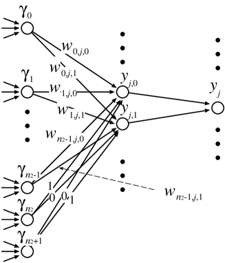
Figure 2: Network structure of a decoder with width $\max(\lceil n/B\rceil+B,BD)$ for $B=2$.

Upon choosing $B=\lceil\sqrt{{\frac{n}{D}}}\rceil$ in Theorem 5 we obtain the following corollary.

Corollary 6.

Suppose $n>D$. Then, for any perfect encoder that maps $X_{n}$ one-to-one to $d$-dimensional binary vectors with $d=\lceil\log n\rceil$, there exists a constant depth perfect decoder width $O(\sqrt{Dn})$ nodes.

Interestingly, this corollary improves the $O(D\sqrt{n})$ size of a perfect decoder given in [8], while using a simpler architecture. Furthermore, the order of this upper bound is close to that of the lower bound given in Theorem 4.

5 Approximate Decoders

In Section 4, we showed a construction of a perfect decoder of width $\max(\lceil n/B\rceil+B,BD)$. It seems not easy to reduce the width using a constant depth. Here we show that we can reduce the width if small errors between the original input vectors (to the encoder) and the output vectors are permissible. This assumption is reasonable because the input and output vectors are not necessarily the same in practice.

In order to measure the error, we employ the Hamming distance between the original vector ${\bf x}$ and the decoded vector ${\bf y}$, and denote it by $dist({\bf x},{\bf y})$. The average Hamming distance $dist(X,Y)$ between the sets of vectors $X=({\bf x}^{0},\ldots,{\bf x}^{n-1})$ and $Y=({\bf y}^{0},\ldots,{\bf y}^{n-1})$ is defined as

$$dist(X,Y)={\frac{1}{n}}\sum_{i=0}^{n-1}dist({\bf x}^{i},{\bf y}^{i}).$$

5.1 Case of $B=3$

As in Section 4, we divide the input vectors into $B$ sets. In this subsection, we consider the case of $B=3$ for ease of presentation. We will extend it to a general $B$ in the next subsection.

We assume w.l.o.g. that ${\frac{n}{3}}$ is a positive integer and define $n_{3}={\frac{n}{3}}$. We construct $\gamma_{i}$ nodes $(i=0,\ldots,n_{3}+2)$, $y_{i,0}$ nodes $(i=0,\ldots,D-1$), and $y_{i,1}$ nodes $(i=0,\ldots,D-1)$ as follows (see Fig. 3).

Recall that $Int(\beta)$ denotes the integer coded by a binary vector $\beta$. Then, the activation function of $\gamma_{i}$ is defined by

$$\gamma_{i} = [\lfloor{\frac{Int(\beta)}{3}}\rfloor=i],~{}~{}~{}~{}\mbox{for $i=0,\ldots,n_{3}-1$},$$

$$\gamma_{n_{3}} = [Int(\beta)=0~{}(\mbox{mod}~{}3)],$$

$$\gamma_{n_{3}+1} = [Int(\beta)=1~{}(\mbox{mod}~{}3)],$$

$$\gamma_{n_{3}+2} = [Int(\beta)=2~{}(\mbox{mod}~{}3)].$$

The activation function for $y_{j,h},j=0,\ldots,D-1,h=0,1$, is

$$y_{j,h}=[\sum^{n_{3}+2}_{i=0}w^{j}_{i,h}\gamma_{i}\geq 0].$$

The values of $w^{j}_{i,h}$s ($i=0,\ldots,n_{3}-1$, $h=0,1$) depend on $x^{3i}_{j}x^{3i+1}_{j}x^{3i+2}_{j}$ and are determined as in Table 1, where each weight $w^{j}_{i,h}$ is shown by its binary representation (e.g., $w^{j}_{i,0}=4$ and $w^{j}_{i,1}=1$ if $x^{3i}_{j}x^{3i+1}_{j}x^{3i+2}_{j}=010$). Note that the corresponding values of the $y_{j,h}$s and $z_{j}$s are also shown in the table. The values of $w^{j}_{i,h}$s ($i=n_{3},n_{3}+1,n_{3}+2$, $h=0,1$) are defined by

$$w^{j}_{{n_{3}},0}=-2, w^{j}_{{n_{3}+1},0}=-4,~{}~{}~{}w^{j}_{{n_{3}+2},0}=0,$$

$$w^{j}_{{n_{3}},1}=-2, w^{j}_{{n_{3}+1},1}=0,~{}~{}~{}~{}w^{j}_{{n_{3}+2},1}=-4,$$

where these $w^{j}_{i,h}$s do not depend on $j$.

Then, for each $j=0,\ldots,D-1$, we construct a node $z_{j}$ with the activation function defined by

$$z_{j}=\left[y_{j,0}+y_{j,1}\geq 2\right].$$

Table 1: Definitions of weight $w^{j}_{i,h}$s and values of relevant variables.

$x^{3i}_{j}x^{3i+1}_{j}x^{3i+2}_{j}$	$w^{j}_{i,0}$	$w^{j}_{i,1}$	$y^{3i}_{j,0}y^{3i+1}_{j,0}y^{3i+2}_{j,0}$	$y^{3i}_{j,1}y^{3i+1}_{j,1}y^{3i+2}_{j,1}$	$z^{3i}_{j}z^{3i+1}_{j}z^{3i+2}_{j}$
000	000	000	001	010	000
001	001	100	001	111	001
010	100	001	111	010	010
011	101	101	111	111	111
100	010	010	101	110	100
101	011	110	101	111	101
110	110	011	111	110	110
111	111	111	111	111	111

We use $w_{h}(\ldots)$ ($h=0,1$) to denote the functions given in the above. For example, $w_{0}(010)=100_{(2)}=4$, $w_{1}(010)=001_{(2)}=1$, $w_{0}(110)=110_{(2)}=6$, and $w_{1}(110)=011_{(2)}=3$, where $x_{(2)}$ means that $x$ is a binary representation of an integer.

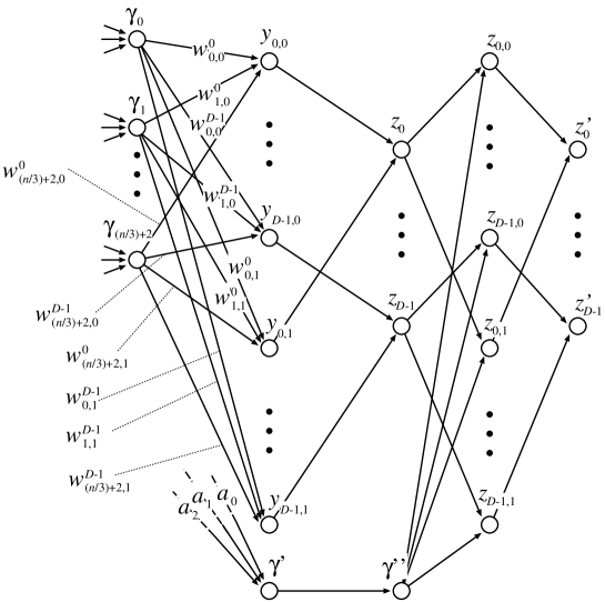
Figure 3: Network structure for approximate decoding with $B=3$.

It is seen from this table that an error occurs only when $x^{3i}_{j}x^{3i+1}_{j}x^{3i+2}_{j}=011$. Therefore, if all bit patterns are distributed uniformly at random, the expected Hamming distance between ${\bf x}^{i}$ and ${\bf y}^{i}$ is ${\frac{D}{3\cdot 2^{3}}}={\frac{D}{24}}$. We can modify the network so that the average Hamming distance between ${\bf x}^{i}$ and ${\bf y}^{i}$ is always no more than ${\frac{D}{24}}$.

This can be done as follows. Let $\#_{b_{0}b_{1}b_{2}}=\sum_{j=0}^{D-1}|\{i|x^{3i}_{j}x^{3i+1}_{j}x^{3i+2}_{j}=b_{0}b_{1}b_{2}\}|$ where $b_{0}b_{1}b_{2}\in\{0,1\}^{3}$. Let $c_{0}c_{1}c_{2}=\mbox{argmin}_{b_{0}b_{1}b_{2}}\#_{b_{0}b_{1}b_{2}}$, where the tie can be broken in any way. Then, we let $a_{0}a_{1}a_{2}=(0\oplus c_{0})(1\oplus c_{1})(1\oplus c_{2})$. For example. $a_{0}a_{1}a_{2}=011$ when $c_{0}c_{1}c_{2}=000$.

Here we define $\chi_{a_{0}a_{1}a_{2}}(x_{0}x_{1}x_{2})$ by

$$\chi_{a_{0}a_{1}a_{2}}(x_{0}x_{1}x_{2})=(x_{0}\oplus a_{0})(x_{1}\oplus a_{1})(x_{2}\oplus a_{2}).$$

For example, $\chi_{011}(000)=011$, $\chi_{011}(001)=010$, and $\chi_{011}(011)=000$ when $a_{0}a_{1}a_{2}=011$. Then, we define $w^{j}_{i,h}$ by

$$w^{j}_{i,0} = w_{0}(\chi_{a_{0}a_{1}a_{2}}(x^{3i}_{j}x^{3i+1}_{j}x^{3i+2}_{j})),$$

$$w^{j}_{i,1} = w_{1}(\chi_{a_{0}a_{1}a_{2}}(x^{3i}_{j}x^{3i+1}_{j}x^{3i+2}_{j})).$$

Finally, we define nodes $z_{j}^{\prime}$ in the output layer by

$$z_{j}^{\prime}=z_{j}\oplus((a_{0}\gamma_{n_{3}})\lor(a_{1}\gamma_{n_{3}+1})\lor(a_{2}\gamma_{n_{3}+2})),$$

which can be realized by adding nodes $\gamma^{\prime}$, $\gamma^{\prime\prime}$, and $z_{j,h}$ ($j=0,\ldots,D-1,h=0,1$) and by defining the activation functions as:

$$\gamma^{\prime} = [a_{0}\gamma_{n_{3}}+a_{1}\gamma_{n_{3}+1}+a_{2}\gamma_{n_{3}+2}\geq 1],$$

$$\gamma^{\prime\prime} = [\gamma^{\prime}\geq 1],$$

$$z_{i,0} = [z_{i}-\gamma^{\prime\prime}\geq 1],$$

$$z_{i,1} = [-z_{i}+\gamma^{\prime\prime}\geq 1],$$

$$z^{\prime}_{i} = [z_{i,0}+z_{i,1}\geq 1].$$

For example, when $c_{0}c_{1}c_{2}=000$, we have the values of relevant variables as in Table 2.

Table 2: Values of relevant variables for the case of $c_{0}c_{1}c_{2}=000$.

$x^{3i}_{j}x^{3i+1}_{j}x^{3i+2}_{j}$	$\chi_{011}(x^{3i}_{j}x^{3i+1}_{j}x^{3i+2}_{j})$	$z^{3i}_{j}z^{3i+1}_{j}z^{3i+2}_{j}$	$(z^{\prime})^{3i}_{j}(z^{\prime})^{3i+1}_{j}(z^{\prime})^{3i+2}_{j}$
000	011	111	100
001	010	010	001
010	001	001	010
011	000	000	011
100	111	111	100
101	110	110	101
110	101	101	110
111	100	100	111

Indeed, if $x^{3i}_{j}x^{3i+1}_{j}x^{3i+2}_{j}=010$, we have $z^{3i}_{j}z^{3i+1}_{j}z^{3i+2}_{j}=001$ and $(z^{\prime})^{3i}_{j}(z^{\prime})^{3i+1}_{j}(z^{\prime})^{3i+2}_{j}=010$ by the following:

$$w^{j}_{i,0} = w_{0}(\chi_{011}(010))=w_{0}(001)=001_{(2)}=1,$$

$$w^{j}_{i,1} = w_{1}(\chi_{011}(010))=w_{1}(001)=100_{(2)}=4,$$

[for $$3i$$:]

$$y_{j,0} = [1-2\geq 0]=0,$$

$$y_{j,1} = [4-2\geq 0]=1,$$

$$z_{j} = [0+1\geq 2]=0,$$

$$z_{j}^{\prime} = 0\oplus(0\cdot\gamma_{n_{3}})=0,$$

[for $$3i+1$$:]

$$y_{j,0} = [1-4\geq 0]=0,$$

$$y_{j,1} = [4-0\geq 0]=1,$$

$$z_{j} = [0+1\geq 2]=0,$$

$$z_{j}^{\prime} = 0\oplus(1\cdot\gamma_{n_{3}+1})=1,$$

[for $$3i+2$$:]

$$y_{j,0} = [1-0\geq 0]=1,$$

$$y_{j,1} = [4-4\geq 0]=1,$$

$$z_{j} = [1+1\geq 2]=1,$$

$$z_{j}^{\prime} = 1\oplus(1\cdot\gamma_{n_{3}+2})=0.$$

If $n$ can be divided by 3, the total error will be at most ${\frac{nD}{3\cdot 2^{3}}}={\frac{nD}{24}}$. Otherwise, the total error will be at most ${\frac{nD}{3\cdot 2^{3}}}={\frac{nD}{24}}+D$ because there might be an additional error per $j$. Since the maximum width is given by $\max(\lceil n/3\rceil+3,2D+1)$, we have the following theorem.

Theorem 7.

For any perfect encoder that maps $X_{n}$ one-to-one to $d$-dimensional binary vectors, with $d=\lceil\log n\rceil$ and $n$ sufficiently large, there exists a decoder of a constant depth and width $\max(\lceil n/3\rceil+3,2D+1)$ whose average Hamming distance error is at most $D({\frac{1}{24}}+{\frac{1}{n}})$.

5.2 General Case

As in Section 4, we define $n_{B}=n/B$ and assume w.l.o.g. that $n$ can be divided by $B$. First, we define $\gamma_{i}$ nodes ($i=0,\ldots,n_{B}+B-1$) by

$$\gamma_{i} = [\lfloor{\frac{Int(\beta)}{B}}\rfloor=i],~{}~{}~{}~{}\mbox{for $i=0,\ldots,n_{B}-1$},$$

$$\gamma_{n_{B}+k} = [Int(\beta)=k~{}(\mbox{mod}~{}B)],~{}~{}~{}~{}\mbox{for $k=0,\ldots,B-1$}.$$

We construct $y_{j,h}$ nodes ($j=0,\ldots,D-1$, $h=0,\ldots,B-2$) and $z_{j}$ nodes ($j=0,\ldots,D-1$) with the activation functions:

$$y_{j,h} = \left[\sum_{i=0}^{n_{3}+B-1}w^{j}_{i,h}\gamma_{i}\geq\theta_{h}\right],$$

$$z_{j} = \left[\sum_{h=0}^{B-2}y_{0,h}~{}\geq~{}B-1\right].$$

We define $w_{n_{B}+i,h}$s ($i=0,\ldots.B-1$, $h=0,\ldots,B-2$) by

$$w_{n_{B}+i,h} = \left\{\begin{array}[]{ll}-{\frac{2^{B}}{4}},&\mbox{if $i=0$ and $h\in\{0,\ldots,B-2\}$},\\ -{\frac{2^{B}}{2}},&\mbox{if $i=h+1$ and $h\in\{0,\ldots,B-2\}$},\\ 0,&\mbox{otherwise},\end{array}\right.$$

For integer $k\in\{0,\ldots,2^{B}-1\}$, let $k_{0}k_{1}\cdots k_{B-1}$ be the binary representation of $k$ (i.e., $k=Int(k_{0}k_{1}\cdots k_{B-1})$), where $k_{0}$ is the most significant bit. We define $w_{h}(k)$ ($h=0,\ldots,B-2$) by

$$w_{0}(k_{0}k_{1}k_{2}k_{3}\cdots k_{B-1}) = Int(k_{1}k_{0}k_{2}k_{3}\cdots k_{B-1}),$$

$$w_{1}(k_{0}k_{1}k_{2}k_{3}\cdots k_{B-1}) = Int(k_{2}k_{0}k_{1}k_{3}\cdots k_{B-1}),$$

$$w_{2}(k_{0}k_{1}k_{2}k_{3}\cdots k_{B-1}) = Int(k_{3}k_{0}k_{1}k_{2}\cdots k_{B-1}),$$

$$\cdots$$

$$w_{B-2}(k_{0}k_{1}k_{2}k_{3}\cdots k_{B-1}) = Int(k_{B-1}k_{0}k_{1}\cdots k_{B-2}).$$

Then, we define $w^{j}_{i,h}=w_{h}(x^{Bi}_{j}x^{Bi+1}_{j}\cdots x^{Bi+B-1}_{j})$ for $j=0,\ldots,D-1$, $i=0,\ldots,n_{B}-1$, and $h=0,\ldots,B-2$. The following proposition is straightforward from the definitions of $y_{i,h}$s, $w_{n_{B}+i,h}$s, $w_{h}(\cdots)$s, and $z_{j}$s.

Proposition 8.

If $x^{Bi}_{j}x^{Bi+1}_{j}x^{Bi+2}_{j}\cdots x^{Bi+B-1}_{j}=011\cdots 1$, then $z^{Bi}_{j}z^{Bi+1}_{j}z^{Bi+2}_{j}\cdots z^{Bi+B-1}_{j}=111\cdots 1$ holds. Otherwise, $z^{Bi}_{j}z^{Bi+1}_{j}z^{Bi+2}_{j}\cdots z^{Bi+B-1}_{j}=x^{Bi}_{j}x^{Bi+1}_{j}x^{Bi+2}_{j}\cdots x^{Bi+B-1}_{j}$ holds.

As in Section 5.1, it is seen from this proposition that if all bit patterns are distributed uniformly at random, the expected Hamming distance between ${\bf x}^{i}$ and ${\bf y}^{i}$ is ${\frac{D}{B2^{B}}}$. We can modify the network so that the average Hamming distance between ${\bf x}^{i}$ and ${\bf y}^{i}$ is always no more than ${\frac{D}{B2^{B}}}$ as well. The modification method is given below, which is almost the same as that in Section 5.1.

Let $\#_{b_{0}b_{1}\cdots b_{B-1}}=\sum_{j=0}^{D-1}|\{i|x^{Bi}_{j}x^{Bi+1}_{j}\cdots x^{Bi+B-1}_{j}=b_{0}b_{1}\cdots b_{B-1}\}|$ where $b_{0}b_{1}\cdots b_{B-1}\in\{0,1\}^{B}$. Let $c_{0}c_{1}\cdots c_{B-1}=\mbox{argmin}_{b_{0}b_{1}\cdots b_{B-1}}\#_{b_{0}b_{1}\cdots b_{B-1}}$, where the tie can be broken in any way. Then, we let $a_{0}a_{1}\cdots a_{B-1}=(0\oplus c_{0})(1\oplus c_{1})\cdots(1\oplus c_{B-1})$. For example. $a_{0}a_{1}a_{2}a_{3}=0110$ when $c_{0}c_{1}c_{2}c_{3}=0001$.

Here we define $\chi_{a_{0}a_{1}\cdots a_{B-1}}(x_{0}x_{1}\cdots x_{B-1})$ by

$$\chi_{a_{0}a_{1}\cdots a_{B-1}}(x_{0}x_{1}\cdots x_{B-1})=(x_{0}\oplus a_{0})(x_{1}\oplus a_{1})\cdots(x_{B-1}\oplus a_{B-1}).$$

Then, we define $w^{j}_{i,h}$ by

$$w^{j}_{i,h} = w_{h}(\chi_{a_{0}a_{1}\cdots a_{B-1}}(x^{Bi}_{j}x^{Bi+1}_{j}\cdots x^{Bi+B-1}_{j})),$$

for $j=0,\ldots,D-1$, $i=0,\ldots,n_{B}-1$, and $h=0,\ldots,B-2$. Finally, we define nodes $z_{j}^{\prime}$ in the output layer by

$$z_{j}^{\prime}=z_{j}\oplus(\bigvee_{h=0}^{B-1}a_{h}\gamma_{n_{B}+h}),$$

which can be realized by adding nodes $\gamma^{\prime}$, $\gamma^{\prime\prime}$, and $z_{j,h}$ ($j=0,\ldots,D-1,h=0,1$) and defining the activation functions by:

$$\gamma^{\prime} = [\sum_{h=0}^{B-1}a_{h}\gamma_{n_{B}+h}~{}\geq~{}1],$$

$$\gamma^{\prime\prime} = [\gamma^{\prime}\geq 1],$$

$$z_{i,0} = [z_{i}-\gamma^{\prime\prime}\geq 1],$$

$$z_{i,1} = [-z_{i}+\gamma^{\prime\prime}\geq 1],$$

$$z^{\prime}_{i} = [z_{i,0}+z_{i,1}\geq 1].$$

Since the maximum width is given by $\max(\lceil n/B\rceil+B,(B-1)D+1)$, we have the following theorem.

Theorem 9.

For any perfect encoder that maps $X_{n}$ one-to-one to $d$-dimensional binary vectors, with $d=\lceil\log n\rceil$ and sufficiently large $n$, there exists a decoder of a constant depth and width $\max(\lceil n/B\rceil+B,(B-1)D+1)$ whose average Hamming distance error is at most $D({\frac{1}{B2^{B}}}+{\frac{1}{n}})$, where $B$ is any integer such that $3\leq B\leq n$.

Note that this theorem is a generalized version of Theorem 7 and the resulting width is smaller than that of Theorem 5 for all $B\geq 3$ and $\lceil n/B\rceil+B>BD$ (i.e., $D<n^{\prime}$ for $n^{\prime}\approx n/B^{2}$) although the corresponding decoder is an approximate one and uses more layers. Note also that if $B=2^{K}$, the architecture of the decoder can be explicitly described as $d/\lceil n/B\rceil+B/(B-1)D+1/D+1/2D/D$ where $d=\lceil\log n\rceil$. Furthermore, if we can consider the average case error over binary input vectors given uniformly at random, this architecture can be reduced to $d/\lceil n/B\rceil+B/(B-1)D/D$.

6 Concluding Remarks

In this paper, we showed an improved upper bound on the size/width of the decoder in a Boolean threshold autoencoder. We also showed a lower bound on the size of the decoder. Although these bounds are relatively close, there still exists a gap. Therefore, closing the gap is left as an open problem as well as giving a lower bound on the size/width of the encoder part. We also constructed decoders that are permitted to make small errors. However, the widths of these decoders are not significantly smaller than those of exact decoders. Therefore, improvement of decoders allowing errors is left as future work.

References

- [1] David H. Ackley, Geoffrey E. Hinton, and Terrence J. Sejnowski. A learning algorithm for boltzmann machines. Cognitive Science, 9:147–169, 1985.
- [2] Martin Anthony. Discrete Mathematics of Neural Networks, Selected Topics. SIAM, 2001.
- [3] Pierre Baldi. Autoencoders, unsupervised learning, and deep architectures. JMLR: Workshop and Conference Proceedings, 27:37–50, 2012.
- [4] Pierre Baldi and Kurt Hornik. Neural networks and principal component analysis:learning from examples without local minima. Neural Networks, 2:53–38, 1989.
- [5] Carl Doersch. Tutorial on variational autoencoders. arXiv, 1606.05908, 2016.
- [6] Rafael Gómez-Bombarelli, Jennifer N. Wei, David Duvenaud, José Miguel Hernández-Lobato, Benjamín Sánchez-Lengeling, Dennis Sheberla, Jorge Aguilera-Iparraguirre, Timothy D. Hirzel, Ryan P. Adams, and Alán Aspuru-Guzik. Automatic chemical design using a data-driven continuous representation of molecules. ACS Central Science, 4(2):268–276, 2018.
- [7] Geoffrey E. Hinton and Ruslan R. Salakhutdinov. Reducing the dimensionality of data with neural networks. Science, 313:504–507, 2006.
- [8] Avraham A. Melkman, Sini Guo, Wai-Ki Ching, Pengyu Liu, and Tatsuys Akutsu. On the compressive power of boolean threshold autoencoders. IEEE Trans. Neural Networks and Learning Systems, in press.
- [9] Kai-Yeung Siu, Jehoshual Bruck, Thomas Kailath, and Thomas Hofmeister. Depth efficient neural networks for division and related problems. IEEE Trans. Information Theory, 39:946–956, 1993.
- [10] Kai-Yeung Siu, Vwani Rndoychowdhury, and Thomas Kailath. Discrete Neural Computation. A Theoretical Foundation. Prentice-Hall, 1995.
- [11] Michael Tschannen, Olivier Bachem, and Mario Lucic. Recent advances in autoencoder-based representation learning. arXiv, 1812.05069, 2018.
- [12] Jiří Šíma and Pekka Orponen. General-purpose computation with neural networks: a survey of complexity theoretic results. Neural Computation, 15:2727–2778, 2003.