Accelerating Clique Counting in Sparse Real-World Graphs via Communication-Reducing Optimizations

Abstract

Counting instances of specific subgraphs in a larger graph is an important problem in graph mining. Finding cliques of size k (k-cliques) is one example of this NP-hard problem. Different algorithms for clique counting avoid counting the same clique multiple times by pivoting or ordering the graph. Ordering-based algorithms include an ordering step to direct the edges in the input graph, and a counting step, which is dominated by building node or edge-induced subgraphs. Of the ordering-based algorithms, kClist is the state-of-the art algorithm designed to work on sparse real-world graphs. Despite its leading overall performance, kClist’s vertex-parallel implementation does not scale well in practice on graphs with a few million vertices.

We present CITRON (Clique counting with Traffic Reducing Optimizations) to improve the parallel scalability and thus overall performance of clique counting. We accelerate the ordering phase by abandoning kClist’s sequential core ordering and using a parallelized degree ordering. We accelerate the counting phase with our reorganized subgraph data structures that reduce memory traffic to improve scaling bottlenecks. Our sorted, compact neighbor lists improve locality and communication efficiency which results in near-linear parallel scaling. CITRON significantly outperforms kClist while counting moderately sized cliques, and thus increases the size of graph practical for clique counting.

We have recently become aware of ArbCount [1], which often outperforms us. However, we believe that the analysis included in this paper will be helpful for anyone who wishes to understand the performance characteristics of k-clique counting.

I Introduction

Clique finding is a well-researched topic in the graph community and it has many interesting practical applications for community detection [2, 3, 4, 5] and social network analysis [6, 7]. In recent years, the data mining community has incorporated clique finding into deep learning classifiers to enhance recommender systems in social networks [8, 9]. Clique finding is used prominently in bioinformatics, and researchers have used graph models to find variants in gene sequences [10], efficiently group related genes in a database [11] and perform protein structure analysis [12]. The rapid growth in the number of social media users and the large size of genome data has amplified the need for high performance systems capable of analyzing these huge networks to count or enumerate their k-cliques.

Clique finding represents only a single problem in Graph Pattern Mining (GPM). Motifs are other general graph patterns that also interest researchers in this space. Various GPM frameworks have been developed to count repeating instances of given patterns within the search graph. These include Pangolin [13], Peregrine [14], Arabesque [15], Fractal [16], and others. The aforementioned frameworks use more generalized algorithms and provide their own APIs for counting instances of arbitrary, user-given patterns. In contrast, there are also algorithms specialized for counting of k-cliques, such as kClist [17], Pivoter [18], and Arb-Count [1]. By virtue of being custom designed to solve a specific problem, these algorithms generally perform better than the general-purpose GPM frameworks.

KClist [17] is the current state-of-the-art clique counting algorithm, as it is algorithmically efficient and significantly outperforms prior work. However, when applied to large graphs, it demonstrates poor parallel scalability, especially for modest clique sizes. We carefully analyze kClist and identify scaling bottlenecks in both of its main phases: ordering & counting. The ordering phase directionalizes the graph in order to avoid redundantly counting the same cliques multiple times in the subsequent counting phase. KClist uses a core ordering [19] to reduce the maximum degree in order to obtain the greatest reduction in the amount of algorithmic work in the counting phase. Since the ordering phase consumes a substantial portion of the execution time, and computing a core ordering is inherently sequential, it limits scalability due to Amdahl’s Law. The parallel speedup of kClist’s counting phase quickly saturates, and we observe speedups as poor as 5$\times$ on 24 cores for certain graphs. We find the counting phase is generally memory-bound due to poor locality and the sheer volume of memory traffic.

We present CITRON (Clique Counting with Traffic Reducing Optimizations), a high performance clique counting algorithm. Due to its better parallel scalability, it significantly outperforms kClist, especially for modest clique sizes. We find the use of a core ordering unnecessary, and a parallelizable ordering such as a degree ordering not only greatly accelerates the ordering phase, but it also results in negligible slowdowns in the counting phase in practice. We accelerate the counting phase with our novel subgraph construction approach which materially reduces the amount of memory accesses and improves their spatial locality.

We evaluate CITRON on a suite of real-world graphs and compare it to kClist and other prior works. For counting triangles, we achieve speedups of $18.16-208.27\times$ (Geometric Mean: $102.436\times$) in the ordering phase and speedups of $1.1-2.6\times$ (Geometric Mean: $1.798\times$) in the counting phase, resulting in total speedups of $14.37-39.37\times$ (Geometric Mean: $18.517\times$) over kClist.

We have recently become aware of ArbCount [1], which outperforms us as seen in Table IV. However, we believe that the analysis included in this paper will be helpful for anyone who wishes to understand the performance characteristics of k-clique counting.

II Background

For a given undirected input graph G, we want to count the number of cliques present of a given size k. A clique is a completely connected subgraph, i.e. each vertex is connected to every other vertex in the subgraph. The input graph consists of a vertex set, V(G), and an edge set, E(G). For a k-clique C present in the input graph, V(C) $\in$ V(G), E(C) $\in$ E(G) and $|$V(C)$|$ = k. Each vertex u in G has a neighborhood, which is the set of the vertices with which u shares an edge. The neighborhood of u in G is indicated by N(u) and its size is the degree $d(u)=|N(u)|$. We treat G as an undirected graph, so $\forall$ v $\in$ N(u), then u $\in$ N(v).

To reduce the amount of work done when counting cliques, ordering-based algorithms transform G into a directed acyclic graph (DAG), which we denote by $\vec{G}$. This step adds work to direct edges to remove cycles in order to avoid counting the same clique multiple times. Consequently, any vertex u in the new DAG can have two types of neighbors: in-neighbors and out-neighbors. In-neighbors are those vertices in N(u) for which u is the destination vertex of the shared edge. Conversely, u’s out-neighbors are those vertices in N(u) where u is the source vertex of the edge. While counting cliques, we only consider the out-neighbors of a vertex u in $\vec{G}$, denoted by $\vec{N(u)}$. The number of out-neighbors of a vertex u is called its out-degree and is written as $\vec{d(u)}$.

Given a total ordering $\omega$, directionalizing transforms the graph G to $\vec{G}$ by removing the edge u $\rightarrow$ v from E(G) if $\omega$(u) $\geq$ $\omega$(v) and keeping only the edge v $\rightarrow$ u in E($\vec{G}$). Edges are thus directed from a lower $\omega$ to a higher $\omega$ vertex. kClist uses a core ordering, which guarantees the lowest maximum out-degree of a vertex in $\vec{G}$. While this approach reduces the amount of work done while counting cliques, it requires a fair bit of effort to compute, and cannot be parallelized [19]. Alternatively, a degree ordering uses the degree to compare vertices and uses the identifier as a tie breaker (example in Figure 1). We describe the degree ordering as:
$\omega:\omega(u)>\omega(v)$ if $(\vec{d(u)}>\vec{d(v)})\lor(\vec{d(u)}=\vec{d(v)})\land(u>v)$

Figure 1: Converting an undirected input graph (left) to directed acyclic graph (right) by a degree-based ordering. Furthermore, the highlighted (red) portion on the right indicates the subgraph induced by vertex 0.

A major step in counting cliques is building a vertex-induced subgraph. The induced subgraph contains the vertices in the neighborhood of the target vertex and any edges between them. The induced subgraph does not include the target vertex itself. The highlighted portion in Figure 1 shows the vertex 0 induced subgraph in the example graph. We denote the subgraph induced by vertex $u$ on $\vec{G}$ to be $\vec{g_{u}}$ with $\vec{V(g_{u})}=N(\vec{u})$ and $\vec{E(g_{u})}=\{(v_{1},v_{2})|(v_{1},v_{2})\in E(\vec{G})\land v_{1}\in N(\vec{u})\land v_{2}\in N(\vec{u})\}$.

III Related Work

One of the fastest sequential algorithms for clique counting is provided by Chiba and Nishizeki [20]. First, it ranks the vertices in descending order of degree. Next, it searches the induced subgraph of each vertex recursively k-2 times where k is the size of the desired clique. Once the recursion is complete, the vertex is removed from the graph to avoid duplicate work. The execution time of this algorithm is $O(kma(G)^{k-2})$, where m is the number of edges in the input graph and a(G) is the arboricity, i.e. the minimum number of forests into which the edges can be partitioned. While the algorithm is simple and efficient, the process of removing vertices from the graph makes it sequential and suboptimal for dealing with the massive real-world graphs of today.

In recent years, more work has been done to parallelize clique counting to boost performance. Danisch et al. present kClist [17], the current state-of-the art parallel algorithm for counting and listing cliques. KClist is able to parallelize the counting step by first converting the input graph into a directed acyclic graph (DAG). Directionalizing the graph ensures kClist counts each clique only once without resorting to sorting the vertices and then removing them one by one sequentially while counting like Chiba and Nishizeki’s algorithm. KClist uses a core ordering to rank vertices for directionalizing the graph to be used in the counting phase. The algorithm for computing the core ordering from Matula and Beck[19] guarantees the smallest maximum out-degree in the graph. This is significant, because the maximum degree determines the execution time of the counting phase and a smaller value means less algorithmic work and a more efficient algorithm.

Algorithm 1 Core Ordering

1:function OrdCore(G)

2:     $r\leftarrow 0,n\leftarrow|V(G)|$

3:     $R\leftarrow[0,0,...,0]$ $\triangleright$ Array to hold rank of each node

4:     while $n\neq 0$ do

5:         Sort nodes by degree

6:         $r\leftarrow r+1$

7:         $minDegNode\leftarrow$ first element from sorted list

8:         $R[minDegNode]\leftarrow n-r$

9:         $V(G)\leftarrow V(G)\setminus{minDegNode}$

10:         Update degrees of all $v\in N(minDegNode)$

11:         $n\leftarrow n-1$      

12:     return $R$

13:Build Graph $\vec{G}$ using $R$

Once the ranking of each vertex is computed (Algorithm 1), the graph is directionalized and edges u $\rightarrow$ v are only included if and only if R(u) $<$ R(v). Similar to Chiba and Nishizeki’s algorithm, producing the core ordering is also sequential since it requires removing a vertex from the graph in each iteration.

After the DAG is generated, kClist starts counting the cliques (Algorithm 2). It recursively builds subgraphs until a certain depth and then adds up the degrees of vertices in the last recursion layer. Since the DAG is not being modified any further, each vertex can be processed in parallel to reduce execution time.

Algorithm 2 kClist Algorithm for Counting k-cliques

1:$count\leftarrow 0$

2:$\vec{G}\leftarrow$ OrdCore($G$) $\triangleright$ Directionalize input graph

3:Counting(k, $\vec{G}$, n)

4:function Counting(l, $\vec{G}$, count)

5:     if l $=$ 2 then

6:         for all nodes in $\vec{g}$ do

7:              $count\leftarrow count+d(node)$          

8:     else

9:         for all nodes $\in$ V($\vec{G}$) in parallel do

10:              Build subgraph $\vec{g_{node}}$

11:              Counting(l-1, $\vec{g_{node}}$, count)               

12:     return $n$

The worst case execution time for kClist is $O(km\frac{c(G)}{2}^{k-2})$, where c(G) is the core value, i.e. the smallest maximum out-degree generated by ordering the vertices. Since c(G) $\leq$ 2a(G)-1, this is an improvement in the execution time over Chiba and Nishizeki for large values of k even without considering parallelization.

Finocchi et al. [21] present a scalable algorithm for counting k-cliques using the MapReduce framework. They use a degree ordering to direct the graph. More recently, Shi et al. [1] present Arb-Count, a new work-efficient parallel algorithm with polylogarithmic span. Aside from the core and degree ordering, they also implement the Barenboim-Elkin [22] and Goodrich-Pszona [23] orderings. Jain and Seshadhri present Pivoter [18], the leading pivoting-based algorithm for k-clique counting. Their algorithm compresses the recursion tree and stores the canonical form as a Succint Clique Tree (SCT), eliminating the need for ordering the graph. Lastly, Almasri et al. [24] implement ordering and pivoting-based k-clique counting algorithms on GPUs. Aside from the aforementioned dedicated solvers, various GPM frameworks [13, 14, 15, 16] are also capable of counting cliques in large graphs. Peregrine [14] is a pattern-aware framework, meaning it can avoid expensive computation by only exploring relevant subgraphs. Peregrine achieves this by analyzing the input pattern (i.e., k-cliques) to develop a search plan and use it to traverse the graph.

IV Parallelizing the Ordering Phase

As mentioned earlier, the counting phase requires the undirected input graph to be converted into a DAG, and kClist uses the core ordering (Algorithm 1) from Matula and Beck [19] to directionalize the graph. It ranks vertices in the graph by their effective degree. The vertices are initially sorted on the basis of their degrees and stored in a min-heap. The top element is popped and assigned the lowest rank (set to the number of vertices currently in the graph). When a vertex is removed from the graph, the degrees of its neighbors are updated and the process repeats until no vertices remain in the graph. Each edge is directed from a lower-ranked vertex to a higher-ranked vertex. This ordering is attractive because it produces the lowest maximum-degree in the graph, allowing the counting phase to theoretically perform closer to its optimal bound. However, the algorithm’s vertex removal and degree update step make it inherently sequential.

We find that using a degree-based ordering both requires less computation than a core ordering and can be parallelized. The degree ordering considers vertices’ original degrees and does not require a sequential process of eliminating vertices one-by-one. To directionalize the graph based on the degree ordering (Algorithm 3), we compare the degree of the two vertices connected by each edge. The edge is directed from the lower-degree vertex to the higher-degree vertex. If the two degrees are equal, then the edge is directed from the vertex with the lower vertex identifier to that with the higher vertex identifier. While each edge can theoretically be considered in parallel, we find vertex-parallelism is sufficient and it simplifies the code. Since our input graph is symmetrized, we only need to do a single check for the degree and vertex identifier comparison.

In theory, a degree-based ordering is not guaranteed to produce the lowest maximum degree, potentially increasing the work required during the counting phase. However, the time required to calculate a degree-based ordering is significantly smaller than that for computing a core ordering, especially after parallelizing. In practice, we find the degree ordering not only does not significantly slow down the counting phase, it can even accelerate it (Table II).

Algorithm 3 Building a DAG using a Degree-Based Ordering in CITRON

1:function GenOrdering(G)

2:     $degrees\leftarrow(0,0,...,0)$

3:     for all u $\in$ V(G) in parallel do

4:         for all v $\in$ N(u) do

5:              if $(d(u)<d(v))\lor(d(u)=d(v)\land u<v)$ then

6:                  $degrees[u]\leftarrow degrees[u]+1$                             

7:     $offsets\leftarrow PrefixSum(degrees)$

8:     for all u $\in$ V(G) in parallel do

9:         for all v $\in$ $\vec{N(u)}$ do

10:              if $(d(u)<d(v))\lor(d(u)=d(v)\land u<v)$ then

11:                  $neighbors[offsets[u]]\leftarrow v$

12:                  $offsets[u]\leftarrow offsets[u]+1$                             

13:     return $\vec{G}$

Graph Abbr. Description $|$V$|$ (M) $|$E$|$ (M) $\vec{d}$ As-Skitter as Internet topology 1.70 22.19 13.1 Wiki-Talk wt Network of Wikipedia users 2.39 9.320 3.9 Orkut or Social network 3.07 234.37 76.3 Cit-Patents cp Citations made by U.S. patents 3.77 16.52 8.8 LiveJournal lj Blogging community 4.00 69.36 17.2 Friendster fr Social network 65.61 3,612.13 28.9

TABLE I: Summary of the properties of input graphs used in the Evaluation. All graphs are symmetrized and taken from SNAP [25].

Graph Core Ordering Degree Ordering Ordering Time Counting Time Total Time Max. Out-Degree Ordering Time Speedup wrt Ordering Time Speedup wrt Counting Time Total Time Max. Out-Degree (1 thread) Core Ordering (96 threads) Core Ordering As-Skitter 1.557 0.396 1.953 222 0.244 6.381 0.025 62.28 0.080 0.105 231 Wiki-Talk 1.409 0.217 1.626 260 0.150 9.393 0.027 52.185 0.120 0.147 340 Orkut 21.981 1.453 23.434 432 3.946 5.570 0.123 178.707 1.265 1.388 535 Cit-Patents 5.839 0.125 5.964 43 0.931 6.272 0.030 194.633 0.152 0.182 77 LiveJournal 6.769 0.264 7.033 426 1.006 6.729 0.038 178.132 0.244 0.282 524 Friendster 880.505 57.377 937.882 334 162.288 5.426 5.051 174.323 31.271 36.322 868

TABLE II: Comparison between time taken to convert the input graph into a DAG using the two different orderings and the associated counting times and maximum out-degrees. The core ordering is guaranteed to produce the lowest maximum out-degree.

V Improving Counting Phase Scalability

To reduce the effect of confounding factors in our experiments, we first implement the kClist algorithm within the GAP Benchmark Suite reference code (gapbs) [26] and we use it as a baseline. The execution time of our implementation differs only $1.27-6.40\%$ from the publicly released kClist code (Mean: $3.72\%$, Variance: $5.98\%$). Our re-implementation effort allows us to systematically look at the impact of optimizations in isolation without also having to consider other differences in the rest of the code bases.

V-A Scaling Bottlenecks in kClist

Our baseline implementation scales poorly for high thread counts (Figure 6) like the released vertex-parallel implementation of kClist. Danisch et al. suggest load-balancing issues that arise from skewed degree distributions in sparse real-world graphs as a possible explanation for the poor scalability of their vertex-parallel algorithm. Through our analysis, we find load imbalance is at most a minor factor, and other bottlenecks hinder scalability to a much greater extent.

To analyze the impact of load imbalance, we both attempt to improve load balance as well as measure the amount of work done by each thread. We sweep various scheduling parameters such as task granularity (chunk sizes) and scheduler types (static, dynamic, cyclic), and we are not able to fully improve parallel scalability. Lumsdaine et al. show that a cyclic distribution (e.g. static schedule with chunk size of 1 in OpenMP) effectively allocates equal work among threads for triangle counting [27]. We test cyclic scheduling with our implementation, and we observe that parallel scaling is only moderately improved (Figure 2).

We measure the work performed by each thread by the number of inner loop iterations because each iteration consists of a uniform amount of work and the number of iterations while processing each vertex is dependent on the number of neighbors of that vertex. With a cyclic distribution, we are able to achieve uniform work distribution among threads. The normalized standard deviation (the ratio of the standard deviation to the mean) of work measured over 24 threads while counting triangles in Cit-Patents is 0.003.

Shifting our analysis to bottom up, performance counter guided profiling with VTune shows memory accesses to be the bottleneck as the baseline code is 49.52% memory bound while counting triangles on Cit-Patents and the CPU is stalled 47.6% of the clock cycles waiting on DRAM. After our optimizations (to be detailed), according to VTune, we reduce the memory bound to 32.92% and stalls due to DRAM to 30.6% for the same task. Due to the success of our interventions, we can confirm that memory is a significant bottleneck of the original code.

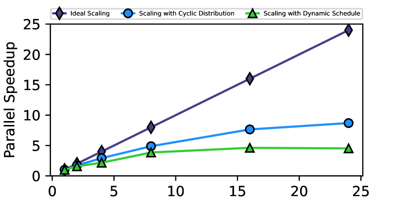
Figure 2: Parallel scaling for counting triangles in Cit-Patents using cyclic work distribution and a dynamic scheduler in the Baseline implementation.

Through our analysis, we find there are three scaling bottlenecks in our baseline implementation that closely mimics kClist. First, the DAG is built in such a way that each directed edge is included twice. This unnecessarily increases the core value, and consequently, the sizes of all the data structures associated with the graph and the subgraph. Scalability is inhibited by allocating a large subgraph structure per thread, and memory accesses quickly become a bottleneck. Second, the original implementation includes a first-level remapping of vertex identifiers changing from the interval $\left[0,|V(G)|-1\right]$ to $\left[0,c(G)-1\right]$ ($c(G)$ is the core value of the graph). We presume this remapping is done to allow the vertex identifier to function as an indexing mechanism to aid in building subgraphs, as well as improving locality. We find that the remapping step increases memory traffic and is not required to accurately count cliques. Lastly, the reference implementation updates a label vector once a neighbor is “visited” so that edges can be included in the subgraph for the following recursion level. This adds an extra memory access while iterating over the neighbor lists. Instead, we find that performing a set intersection of the sorted neighbor arrays is far more efficient. We find that the aforementioned implementation details place a heavy burden on memory by requiring more accesses with poor locality. By fixing these issues in the next subsection, we are able to significantly improve scalability and thus execution time.

V-B Communication Reducing Optimizations

We introduce a number of optimizations to reduce the aforementioned scaling bottlenecks. First, we build our DAG without including duplicate edges and then build compressed adjacency lists for the subgraphs in the subsequent recursion levels. We remove the relabeling step while building the first-level subgraph as well as the label-based intersection from kClist, and replace it with a set-based intersection on sorted neighbor lists. Finally, we implement certain heuristics to further reduce the amount of work done in the counting phase.

Compressing the Adjacency List

As opposed to kClist (which contains two copies of each edge), our generated DAG contains sorted adjacency lists without duplicate neighbors. This becomes beneficial while building the subgraphs during recursion, since we can simply append each new neighbor to the end of the array. kClist pessimistically reserves $c(G)$ spaces per node in the subgraph and then starts placing the neighbors of the $i^{th}$ neighbor at index $i\times c(G)$, making the adjacency list large and sparsely filled since all entries between indices $i\times c(G)+d(\vec{i})$ and $(i+1)\times c(G)$ are unused (Figure 4). This inevitably leads to poor locality and increased cache misses. We can see the stark difference in how much memory is used for storing the first level subgraph by kClist and CITRON in Table III. We describe both subgraph building methods in more detail in Section 5.2.2.

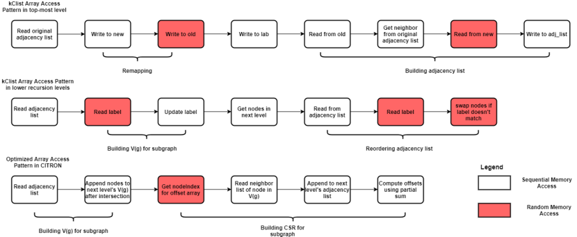
Figure 3: Memory Access Patterns for the reference kClist implementation and CITRON. The optimized version requires fewer random accesses as well as less memory accesses overall, improving performance.

Reducing Memory Traffic by Removing Label Array

The main step of the subgraph building process is finding which edges will exist in the subgraph by intersecting each vertices’ neighbor list in the original graph with $\vec{V(g)}$. KClist accomplishes this by having a single label vector with an entry per node (Algorithm 4). The algorithm then loops over each node’s neighbor list in the subgraph twice. Initially, there is a check to see if the label of the neighbor is equal to the current recursion level l (Step 3). If it is equal, then the vertex has been accessed for the first time so it is added to the vertex set of the subgraph for the next level (Step 5 ) and updated to l-1 (Step 6). The second loop finds edges and updates the degrees of each node in the new vertex set. This is done by iterating over each neighbor’s neighbor list and checking their label. If the label is l-1, then an edge is present and the degree of the neighbor is incremented (Step 10).

Algorithm 4 Building an Induced Subgraph in kClist

1:function GenSubgraph($\vec{G}$, l, u)

2:     $V(\vec{g_{u}})=\phi$

3:     for all $nodes\in$ $\vec{N(u)}$ do

4:         if $lab[node]=l$ then

5:              add $node$ to V($\vec{g_{u}}$)

6:              $lab[node]\leftarrow l-1$               

7:     for all $node$ $\in$ V($\vec{g_{u}}$) do

8:         for all $neighbor$ $\in$ $\vec{N(node)}$ do

9:              if $lab[neighbor]=l-1$ then

10:                  $\vec{d(node)}\leftarrow\vec{d(node)}+1$

11:              else

12:                  Swap nodes in adjacency list                        

13:         Reset all labels to l      

14:     return $\vec{g_{u}}$

Step 11 (Algorithm 4) is an optimization Danisch et al. [17] mention explicitly in their paper. All the out-neighbors of a node in the next level subgraph are moved to the start of that node’s neighborhood in the original adjacency list. This further increases the number of data writes required.

One of our major contributions in CITRON is eliminating extra memory accesses for the remapping and the label-based intersection while building subgraphs (Algorithm 5). By having a separate adjacency list and offset array for each subgraph layer, our data is more tightly packed in contrast to the spread out, sparse structure for kClist. Instead of reading and writing from a label array (with poor locality) to check for common neighbors, we perform set intersections between V(G) and $\vec{N(u)}$. Since our original DAG is sorted, these intersections are very efficient. Building the adjacency list only requires us to append each neighbor to the end of the existing array as we go. Since we sort the DAG in the original graph, we ensure that the individual neighbor lists in the subsequent adjacency list are also sorted without doing any extra work. Furthermore, storing each subgraph separately removes the need for swapping nodes and eliminates extra writes.

Algorithm 5 Optimized Subgraph Building in CITRON

1:function GenSubgraph($\vec{G}$, l, u)

2:     $\vec{V(g_{u})}=\vec{N(u)}$

3:     for all node $\in$ $\vec{V(g_{u})}$ do

4:         for all neighbor $\in$ $\vec{N(node)}$ do

5:              outEdges $\leftarrow$ $\vec{V(g_{u})}$ $\cap$ $\vec{N(neighbor)}$

6:              $adjList.append(outEdges)$

7:              $\vec{d(node)}\leftarrow\vec{d(node)}+|outEdges|$

8:              $offsets\leftarrow PartialSum(d)$ $\triangleright$ for CSR               

9:     return $\vec{g_{u}}$

To contrast the graph structures of the two approaches and how it impacts locality, we illustrate the example from Figure 1 for both kClist (Figure 4) and CITRON (Figure 5).

The adjacency list for kClist contains $c(G)$ entries reserved for each potential neighbor, i.e. $c(G)\times c(G)$ entries in total. The value of $c(G)$ for the example graph from Figure 1 is 3. For simplicity, we assume that the neighbor lists in the DAG are sorted and there are no duplicate entries. After the initial remapping phase, the new vertex identifiers are {0, 1, 2}.

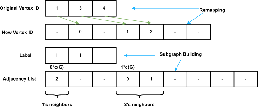
Figure 4: First level subgraph for example graph (Figure 1) in the baseline implementation. There is also a separate array for storing the degrees of each vertex in the subgraph not pictured.

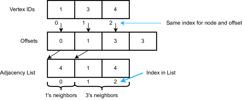
Figure 5: First level subgraph for example graph (Figure 1) in CITRON. There is also a separate array for storing the degrees of each vertex in the subgraph not pictured.

For high-degree vertices, we can see how kClist’s organization can be wasteful and require multiple accesses to fit the entire adjacency list into the cache, especially if there are more entries than a cache line can fit. KClist only does the remapping in the top-most recursion level and then swaps nodes to the front of that vertex’s allocated space ($i\times c(G)$). In contrast, our approach skips the remapping and simply appends each vertex’s common neighbors to the end of the array. To get the required neighbor list for the intersection, we can simply slice the adjacency list from indices Offset[nodeIndex] to Offset[nodeIndex+1], where nodeIndex is the index of the vertex in $V(G)$. Our compact adjacency list is similar to the Doubly Compressed Sparse Row (DCSR) format in CombBLAS [28, 29]. Additionally, a simple building process allows us to repeat it per level instead of swapping vertices and still enjoy a performance boost.

Our optimizations in CITRON greatly reduces the memory access and size requirements. Table III compares the number of array accesses required to build all of the first level subgraphs and the total memory (in bytes) used by the largest subgraph in each kClist and CITRON. The kClist subgraph is of a constant size for each vertex since the array lengths are determined by the core value. In contrast, CITRON has a variable subgraph size for each vertex since the adjacency list is built by appending neighbors to the end of a list. To maintain fairness, we report the size of the largest subgraph (induced by the vertex with the highest degree).

Graph Baseline CITRON Array Accesses Size of Subgraph Array Accesses Size of Subgraph (Billions) (MB) (Billions) (MB) as 3.179 13.775 0.565 0.055 wt 2.594 19.433 0.269 0.080 or 59.186 25.340 19.872 0.092 cp 0.562 30.207 0.305 0.003 lj 9.222 33.030 2.724 0.070 fr 1,011.843 999.145 392.626 0.045

TABLE III: Comparison between the number of array accesses while building all the first level subgraphs and the memory consumed for the baseline and CITRON. We measure sizes with sizeof

From Table III, we observe that CITRON requires fewer array accesses for all of the input graphs. We can also see that the difference in the memory sizes is quite significant, and removing the relabeling step and the label array (used for the intersections) allows us to save additional space in memory. Although the original input graph is far larger than the space reclaimed with our smaller subgraph data structures, its benefit is that it reduces the working set of memory accesses, allowing for more to fit in cache. Additionally, since each thread gets its own private copy of the subgraph struct, the memory required for storing the kClist subgraph can quickly become a bottleneck for high thread counts.

Other Optimizations

We add a heuristic to skip processing nodes if cliques are impossible to be found. If the number of nodes in the subgraph is less than $(l-2)$ at any level in the recursion, then that subgraph will never contain a k-clique.

Finally, we further decrease the amount of work done by not building an adjacency list and computing the row offsets in the penultimate recursion layer. This is possible because we only require degrees of each node in the subgraph in the current level instead of the nodes and their neighbors in the next level. This also reduces the amount of memory required for the last level subgraph.

VI Experimental Setup

VI-A Environment

We perform our experiments on a dual-socket Intel Xeon Platinum 8260. Each socket has 24 physical cores running at 2.40GHz with two-way hyperthreading (48 threads) and 35.75MB shared L3 cache. Our system has 768 GB RAM. For the experiments, we use all thread contexts (96) unless specified otherwise. We compile with g++ (version 9.3.0) with optimization -O3 and use OpenMP. We also use Intel VTune for analyzing our optimization’s improvements.

VI-B Graphs in this Work

We use a variety of input graphs to evaluate the performance of our optimizations (Table I). These graphs are taken from Stanford Network Analysis Project (SNAP) [25]. Since clique finding is used heavily in social network analysis, we have selected commonly used graphs to make analysis more germane. All graphs are unweighted and symmetrized to initially be undirected.

VII Evaluation

In this section, we analyze how the two different orderings affect performance. We also compare the overall performance of our optimizations in CITRON with both vertex-parallel and edge-parallel versions of kClist, as well as a GPM framework in Peregrine [14], a dedicated solver in Pivoter [18], and a recently released code ArbCount [1]. All of the thread scaling experiments are performed by increasing the number of threads (and cores) from 1 to 48. All other comparisons are performed using all available threads (96). We perform at least 2 trials and record the mean for each data point.

VII-A Ordering Comparison

As seen in Table II, a degree-based ordering may not always produce the lowest maximum-degree value. However, its lightweight computation and parallelizability generally lead to overall lower total execution times for clique counting. In Table II, we also break down the ordering and counting times for counting triangles (k=3) in each graph and see how each ordering impacts the total execution time. Both orderings are applied on our optimized code running on 96 threads and the fastest total time is denoted in bold.

The ordering time and total execution time are greatly improved with the parallel degree-based ordering. Additionally, we observe that the counting time for the degree-based ordering is also less in most cases. To understand this, we make a simple model for algorithmic work and animate it with data from our executions. For triangles, the total work is given by the sum of the product of each vertex’s degree with the sum of each of it’s neighbor’s degrees as the algorithm traverses those edges ($\sum_{u\in V(G)}(d_{u}.\sum_{v\in N(\vec{u})}d_{v})$). The degree-based ordering produces a smaller value for work than the core value in most cases. As k gets larger, core ordering becomes more beneficial. Increasing k increases the max recursive depth, and the overall execution becomes more dominated by the highest degree nodes.

VII-B Parallel Scaling of the Counting Phase

To compare the improvement in parallel scaling of our optimizations with our baseline implementation, we count 3,4,5 and 6-cliques on the input graphs on increasing thread counts up to 48 threads (Figure 6). We do not see major improvement using hyperthreading, so we report data using 48 threads on 2 sockets and 1-24 threads on one socket. Each plot shows the parallel speedup of the counting phase relative to single thread of that implementation.

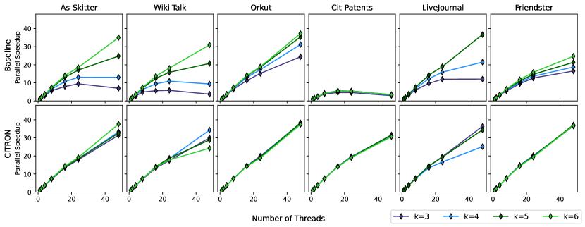
Figure 6: Comparing parallel scaling between the baseline and CITRON for counting cliques of various sizes in all input graphs. All the subplots on the top row are for the baseline implementation and the all the subplots on the bottom row are for CITRON. The graphs are: (left to right) As-Skitter, Wiki-Talk, Orkut, Cit-Patents, LiveJournal, Friendster. At least two trials were completed and the mean was taken to account for variance. Scaling for 6-cliques on LiveJournal is not included as the single-thread runtime is very high.

In the baseline scaling plots (Figure 6), we observe that scaling improves as k increases. We believe the amortization of scheduling overhead causes this phenomenon since more work is required to count larger cliques than smaller cliques. We can see that our optimizations in CITRON reduce this effect. Especially in Orkut and cit-Patents, all k values scale equally well. Most notably, our optimizations perform extremely well compared to kClist on cit-Patents, where we achieve near-linear scaling.

VII-C Total execution time Comparison

Table IV shows the overall execution times for counting cliques of various sizes on all the input graphs for each implementation. We use the released implementation of kClist rather than our baseline for fairness. We were unable to convert As-Skitter into the required graph format for Peregrine. After repeated effort, we are unable to use KClist’s Edge-Parallel implementation to count triangles on any graph. Peregrine is unable to count cliques of any size on Friendster as it times out.

Graph	Algorithm	k=3	k=4	k=5	k=6	k=7	k=8
As-Skitter	CITRON	0.109	0.159	0.410	2.383	20.754	187.908
	kClist Vertex-Parallel	2.358	2.380	2.636	4.508	18.438	115.348
	kClist Edge-Parallel	-	4.273	4.502	6.368	20.240	111.984
	ArbCount	0.0470	0.073	0.127	0.635	5.280	39.699
	Pivoter	30.000	32.667	35.333	37.000	39.000	39.667
Wiki-Talk	CITRON	0.217	0.240	0.399	1.442	6.152	22.925
	kClist Vertex-Parallel	1.638	1.653	1.788	2.383	4.430	10.131
	kClist Edge-Parallel	-	2.792	2.935	3.494	5.534	11.048
	ArbCount	0.042	0.045	0.092	0.468	2.288	8.747
	Peregrine	0.928	10.405	68.781	719.048	$>$1h	$>$1h
	Pivoter	32.667	36.000	40.667	43.333	44.000	46.000
Orkut	CITRON	1.437	3.163	10.043	39.441	170.447	763.592
	kClist Vertex-Parallel	44.442	46.318	52.980	78.320	184.128	624.370
	kClist Edge-Parallel	-	77.152	83.748	110.199	218.507	672.369
	ArbCount	1.201	1.614	2.863	8.694	33.278	133.695
	Peregrine	7.362	144.532	1587.830	$>$1h	$>$1h	$>$1h
	Pivoter	227.333	308.667	400.667	481.333	525.333	583.333
Cit-Patents	CITRON	0.187	0.197	0.206	0.216	0.231	0.243
	kClist Vertex-Parallel	9.918	9.867	9.876	9.894	9.904	9.868
	kClist Edge-Parallel	-	14.128	14.108	14.136	14.098	14.114
	ArbCount	0.122	0.204	0.190	0.181	0.174	0.164
	Peregrine	0.349	0.419	0.415	0.512	1.070	1.599
	Pivoter	62.667	63.000	63.000	63.333	63.667	63.000
LiveJournal	CITRON	0.379	0.896	21.475	980.062	$>$1h	$>$1h
	kClist Vertex-Parallel	9.400	9.666	17.107	378.124	$>$1h	$>$1h
	kClist Edge-Parallel	-	15.212	23.338	371.418	$>$1h	$>$1h
	ArbCount	0.204	0.416	5.587	256.241	$>$1h	$>$1h
	Peregrine	0.537	5.474	218.286	$>$1h	$>$1h	$>$1h
	Pivoter	118.500	299.500	1500.000	$>$1h	$>$1h	$>$1h
Friendster	CITRON	37.790	46.825	65.201	106.352	258.574	1765.970
	Baseline∗	1275.195	1278.400	1281.445	1292.870	1311.890	1354.710
	ArbCount	31.288	70.010	70.817	74.418	93.549	385.024
	Pivoter	4314.500	4433.500	4489.500	4554.500	4537.500	4556.500

TABLE IV: Summary of total execution time for counting cliques using kClist [17], CITRON, Peregrine [14] and Pivoter [18]. Each algorithm was executed using 96 threads on the same machine under the same conditions. The best execution time is denoted in bold. The best execution time other than ArbCount is italicized. ^∗Both Node Parallel and Edge Parallel version of kClist segfaulted for Friendster so we report the values for our baseline implementation which has nearly identical performance to the kClist Node Parallel implementation.

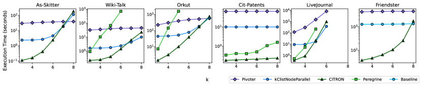
Figure 7: Plots in linlog scale comparing the total execution time required for counting cliques of different sizes on the input graphs using kClist [17], CITRON, Peregrine [14] and Pivoter [18]. kClistEdgeParallel is not included as kClistNodeParallel outperforms it for every graph. As kClist segfaults on Friendster, we include the times of our baseline implementation. On LiveJournal, none of the frameworks are unable to count 7, 8-cliques within an hour.

Our speedups range from $0.39-53.04\times$ (Geometric Mean: $6.19\times$) over kClist, $1.42-498.65\times$ (Geometric Mean: $10.71\times$) over Peregrine and $0.21-335.12\times$ (Geometric Mean: $45.08\times$) over Pivoter. CITRON performs best for modest values of k (Figure 7). The newly released ArbCount outperforms all frameworks most of the time.

We observe that a degree ordering greatly improves the execution time for smaller k values as the overhead of computing the core ordering is very large compared to the counting time. However, as counting time increases with the clique size, this overhead becomes amortized and the core ordering leads to a smaller execution time. This is consistent with Shi et al.’s findings [1].

We suspect that load imbalance likely becomes an issue with our optimizations for higher k values. With a degree-based ordering, the larger maximum degree increases the computational fan-out for building subgraphs in deeper recursions. Our asymptotic analysis also shows that the execution time of the counting phase also grows exponentially for increasing k. We parallelize a task size of 1 (i.e. each vertex). Initial analysis shows counting cliques in the induced subgraphs of large degree vertices require a significant fraction of the total execution time. Thus, it may be beneficial to parallelize subgraph building or further recursion levels for large degree vertices.

VIII Conclusion

CITRON optimizes kClist’s vertex-parallel algorithm by optimizing memory communication and increasing parallelization, both proven techniques to improve graph algorithm performance [30]. CITRON reduces communication between the CPU and memory by more efficiently storing and accessing the subgraph structures in each recursion level of the counting phase. We are able to significantly improve parallel scaling and the time required to count cliques using this optimization. We also use a parallel, lightweight degree-based ordering to produce a DAG in the ordering phase. Even though we lose some efficiency in the counting phase by using the degree-based ordering instead of a core ordering, we observe improvements in total execution time because the degree ordering is faster to compute. CITRON achieves speedups of $18.16-208.27\times$ (Geometric Mean: $102.436\times$) in the ordering phase and speedups of $1.1-2.6\times$ (Geometric Mean: 1.798$\times$) in the counting phase, resulting in total speedups of $14.37-39.37\times$ (Geometric Mean: $18.517\times$) over kClist while counting triangles.

While we focus on counting in this work, we are easily able to enumerate each clique with a few simple changes to our code. Since more research is in the field of Graph Pattern Mining, we hope that our optimization can be used as a performance benchmark to compare the performance of new clique counting algorithms.

References

- [1] J. Shi, L. Dhulipala, and J. Shun, “Parallel clique counting and peeling algorithms,” in SIAM Conference on Applied and Computational Discrete Algorithms (ACDA21). SIAM, 2021, pp. 135–146.
- [2] E. Gregori, L. Lenzini, and S. Mainardi, “Parallel k-clique community detection on large-scale networks,” IEEE Transactions on Parallel and Distributed Systems, vol. 24, no. 8, pp. 1651–1660, 2013.
- [3] G. Palla, I. Derényi, I. Farkas, and T. Vicsek, “Uncovering the overlapping community structure of complex networks in nature and society,” nature, vol. 435, no. 7043, pp. 814–818, 2005.
- [4] F. Hao, G. Min, Z. Pei, D.-S. Park, and L. T. Yang, “-clique community detection in social networks based on formal concept analysis,” IEEE Systems Journal, vol. 11, no. 1, pp. 250–259, 2017.
- [5] Y. Fang, K. Yu, R. Cheng, L. V. Lakshmanan, and X. Lin, “Efficient algorithms for densest subgraph discovery,” arXiv preprint arXiv:1906.00341, 2019.
- [6] L. Pan and E. E. . Santos, “An anytime-anywhere approach for maximal clique enumeration in social network analysis,” in 2008 IEEE International Conference on Systems, Man and Cybernetics, 2008, pp. 3529–3535.
- [7] R. A. Rossi, D. F. Gleich, and A. H. Gebremedhin, “Parallel maximum clique algorithms with applications to network analysis,” SIAM Journal on Scientific Computing, vol. 37, no. 5, pp. C589–C616, 2015.
- [8] S. Manoharan and Sathish, “Patient diet recommendation system using k clique and deep learning classifiers,” Journal of Artificial Intelligence and Capsule Networks, vol. 2, no. 2, pp. 121–130, 2020.
- [9] K. X. P. Vilakone and D. Park, “Personalized movie recommendation system combining data mining with the k-clique method,” Journal of Information Processing Systems, vol. 15, no. 5, pp. 1141–1155, Oct. 2019.
- [10] T. Marschall, I. G. Costa, S. Canzar, M. Bauer, G. W. Klau, A. Schliep, and A. Schönhuth, “CLEVER: clique-enumerating variant finder,” Bioinformatics, vol. 28, no. 22, pp. 2875–2882, 10 2012. [Online]. Available: https://doi.org/10.1093/bioinformatics/bts566
- [11] E. T. T. Matsunaga, C. Yonemori and M. Muramatsu, “Clique-based data mining for related genes in a biomedical database,” BMC Bioinformatics, vol. 10, no. 205, 2009.
- [12] K. C. D. Bahadur, T. Akutsu, E. Tomita, T. Seki, and A. Fujiyama, “Point matching under non-uniform distortions and protein side chain packing based on an efficient maximum clique algorithm,” Genome Informatics, vol. 13, pp. 143–152, 2002.
- [13] X. Chen, R. Dathathri, G. Gill, and K. Pingali, “Pangolin: An efficient and flexible graph mining system on cpu and gpu,” Proceedings of the VLDB Endowment, vol. 13, no. 8, pp. 1190–1205, 2020.
- [14] K. Jamshidi, R. Mahadasa, and K. Vora, “Peregrine: a pattern-aware graph mining system,” in Proceedings of the Fifteenth European Conference on Computer Systems, 2020, pp. 1–16.
- [15] C. H. Teixeira, A. J. Fonseca, M. Serafini, G. Siganos, M. J. Zaki, and A. Aboulnaga, “Arabesque: a system for distributed graph mining,” in Proceedings of the 25th Symposium on Operating Systems Principles, 2015, pp. 425–440.
- [16] V. Dias, C. H. Teixeira, D. Guedes, W. Meira, and S. Parthasarathy, “Fractal: A general-purpose graph pattern mining system,” in Proceedings of the 2019 International Conference on Management of Data, 2019, pp. 1357–1374.
- [17] M. Danisch, O. Balalau, and M. Sozio, “Listing k-cliques in sparse real-world graphs,” in Proceedings of the 2018 World Wide Web Conference, 2018, pp. 589–598.
- [18] S. Jain and C. Seshadhri, “The power of pivoting for exact clique counting,” in Proceedings of the 13th International Conference on Web Search and Data Mining, 2020, pp. 268–276.
- [19] D. W. Matula and L. L. Beck, “Smallest-last ordering and clustering and graph coloring algorithms,” Journal of the ACM (JACM), vol. 30, no. 3, pp. 417–427, 1983.
- [20] N. Chiba and T. Nishizeki, “Arboricity and subgraph listing algorithms,” SIAM Journal on computing, vol. 14, no. 1, pp. 210–223, 1985.
- [21] I. Finocchi, M. Finocchi, and E. G. Fusco, “Clique counting in mapreduce: Algorithms and experiments,” Journal of Experimental Algorithmics (JEA), vol. 20, pp. 1–20, 2015.
- [22] L. Barenboim and M. Elkin, “Sublogarithmic distributed mis algorithm for sparse graphs using nash-williams decomposition,” Distributed Computing, vol. 22, no. 5-6, pp. 363–379, 2010.
- [23] M. T. Goodrich and P. Pszona, “External-memory network analysis algorithms for naturally sparse graphs,” in European Symposium on Algorithms. Springer, 2011, pp. 664–676.
- [24] M. Almasri, I. E. Hajj, R. Nagi, J. Xiong, and W. mei Hwu, “K-clique counting on gpus,” 2021.
- [25] J. Leskovec and A. Krevl, “SNAP Datasets: Stanford large network dataset collection,” http://snap.stanford.edu/data, Jun. 2014.
- [26] S. Beamer, K. Asanović, and D. Patterson, “The gap benchmark suite,” arXiv preprint arXiv:1508.03619, 2015.
- [27] A. Lumsdaine, L. Dalessandro, K. Deweese, J. Firoz, and S. McMillan, “Triangle counting with cyclic distributions,” in 2020 IEEE High Performance Extreme Computing Conference (HPEC). IEEE, 2020, pp. 1–8.
- [28] A. Buluc and J. R. Gilbert, “On the representation and multiplication of hypersparse matrices,” in 2008 IEEE International Symposium on Parallel and Distributed Processing. IEEE, 2008, pp. 1–11.
- [29] A. Buluç and J. R. Gilbert, “The combinatorial blas: Design, implementation, and applications,” The International Journal of High Performance Computing Applications, vol. 25, no. 4, pp. 496–509, 2011.
- [30] S. Beamer, “Understanding and improving graph algorithm performance,” Ph.D. dissertation, University of California, Berkeley, 2016.