Abstract

The Wheeler-DeWitt equation for a Kantowski-Sachs metric in Hořava-Lifshitz gravity with a set of coordinates in minisuperspace that obey a generalized uncertainty principle is studied. We first study the equation coming from a set of coordinates that obey the usual uncertainty principle and find analytic solutions in the infrared as well as a particular ultraviolet limit that allows us to find the solution found in Hořava-Lifshitz gravity with projectability and with detailed balance but now as an approximation of the theory without detailed balance. We then consider the coordinates that obey the generalized uncertainty principle by modifying the previous equation using the relations between both sets of coordinates. We describe two possible ways of obtaining the Wheeler-DeWitt equation. One of them is useful to present the general equation but it is found to be very difficult to solve. Then we use the other proposal to study the limiting cases considered before, that is, the infrared limit that can be compared to the equation obtained by using general relativity and the particular ultraviolet limit. For the second limit we use a ultraviolet approximation and then solve analytically the resulting equation. We find that and oscillatory behaviour is possible in this context but it is not a general feature for any values of the parameters involved.

1 Introduction

Although we do not yet have a complete description of a theory of quantum gravity, there have been enormous efforts from very different points of view, that has brought us closer to an understanding of the gravitational phenomena in a quantum regime. For example, there are now some features that are expected to be found in such a theory. One of the main features that we expect from a quantum theory of gravity is the existence of a minimal measurable length. This idea has arisen in a number of approaches to quantum gravity ranging from string theory [1, 2] to general thought experiments of black holes physics [3, 4] to name a few (see for example [5] for a more thorough discussion). One of the features of the hypothesis of the existence of a minimal length is a modification of the Heisenberg uncertainty principle and thus a generalization of the Heisenberg algebra, known as the Generalized Uncertainty Principle (GUP). This proposal has been extensively studied in the literature from the purely theoretical point of view such as in Refs. [6, 7, 8], as well as from attempts to constraint the parameters involved using well measured quantities from both the classical as well as the quantum point of view, for example see Refs. [9, 10, 11, 12, 13, 14, 15, 16], and even on experimental grounds such as Ref. [17]. These effects are expected to be relevant on systems at very high energies (or short distances) and therefore they are expected to be of first importance in the early universe and quantum effects of black holes. One of the main tools to our disposal to approach the quantum behaviour of gravity is the well known tools of canonical quantization that leads to the Wheeler-DeWitt (WDW) equation [18, 19, 20] and therefore it is natural to study the effects of a GUP in this framework. In fact, recently the effects of considering a GUP to the coordinates in the minisuperspace for a Kantowsi-Sachs metric in the context of the WDW equation was introduced in [21]. For a short overview on this topic the reader can consult Ref. [22]. It has also been studied recently a comparison between considering a GUP and Polymer Quantum Mechanics in a semiclassical as well as quantum approaches in [23].

On the other hand, it is well known that General Relativity (GR) is a non-renormalizable theory and thus looking for quantum aspects of gravity using this theory has a limiting nature. Apart from the search of a full theory of quantum gravity, there has been very interesting approaches that seek to generalize GR by modifying it so it has a better behaviour in the ultraviolet. One of the most important proposals on this regard is the Hořava-Lifshitz (HL) theory of gravity [24] (for some recent reviews, see [25, 26, 27, 28] and references therein). This theory employs an anisotropic scaling of space and time variables, inspired by the Lifshitz scaling of the condensed matter physics, which breaks the Lorentz symmetry of GR and introduces spatial higher-derivative terms to the action of gravity in order to achieve a power counting renormalizable theory. Since this theory represents an improvement in the ultraviolet behaviour of GR, the theory has been studied extensively in the context of canonical quantization, that is regarding the WDW equation, for example see Refs. [29, 30, 31, 32, 33, 34, 35]. Although the non-projectable version of the theory has advantages over the projectable version in particular regarding the infrared limit of the theory, it is also well known that when working with the WDW equation both approaches are completely equivalent and the infrared instability is not detected at this level and therefore in this work we will use the projectable theory. However in the most general case, this perturbative instability leads to the existence of an additional degree of freedom, which does not allow to recover GR (see for instance, [35] for an explanation).

Since HL theory is expected to produce a better quantum behaviour than GR and the GUP is an expected feature of quantum gravity, it is natural to consider both of them in the same approach. A possible connection between these two proposals has been previously studied in Refs. [36, 37]. However, in the present article we are going to consider both proposals as independent. We are going to study the effects of considering a GUP in the WDW equation obtained in the context of HL gravity for a Kantowski-Sachs (KS) metric, considering therefore two contributions in the ultraviolet quantum gravity behaviour in the WDW equation. Thus we will generalize the proposal used for GR in [21].

The present work is organized as follows. In Section 2 we are going to study the standard WDW equation (that is with coordinates that obey the usual uncertainty principle) for a Kantowski-Sachs metric in HL gravity. We will particularly focus on two regimes, the infrared (IR) limit and a special case in the ultraviolet (UV) limit that leads to an analytic solution. In Section 3 we will consider a new set of variables that obeys a GUP and we will show how the WDW equation is obtained in this context, we will present two equivalent ways to deduce such equation. Since the resulting equation is far quite difficult to solve, in Section 4 we will consider the two simple cases considered previously, that is, the IR limit and the particular UV limit. The IR limit can be compared to the case considered in [21] using GR. In the UV limit we look for analytic solutions and we present some figures where we plot the resulting behaviour. Finally, in Section 5 we present our conclusions and final remarks.

2 Wheeler-DeWitt equation in Hořava-Lifshitz gravity

In this section we are going to study the WDW equation coming from a Kantowski-Sachs metric in HL gravity with the usual uncertainty relation. We will study its UV and IR limits, taking special interest in cases in which analytic solutions can be obtained.

We begin by considering the gravitational action in projectable HL gravity without detailed balance. This action can be written as [29, 38, 39]

$$S=\frac{M^{2}_{pl}}{2}\int_{M}d^{3}xdtN\sqrt{h}\left[K_{ij}K^{ij}-\lambda K^{2}-\Lambda M^{2}_{pl}+R-\frac{1}{M^{2}_{pl}}\left(g_{2}R^{2}+g_{3}R_{ij}R^{ij}\right)\right.\\ \left.-\frac{1}{M^{4}_{pl}}\left(g_{4}R^{3}+g_{5}RR^{i}_{j}R^{j}_{i}+g_{6}R^{i}_{j}R^{j}_{k}R^{k}_{i}+g_{7}R\nabla^{2}R+g_{8}\nabla_{i}R_{jk}\nabla^{i}R^{jk}\right)\right]\\ +M^{2}_{pl}\int_{\partial M}d^{3}x\sqrt{h}K,$$ (1)

where $N$ is the lapse function, $\lambda$ is a running parameter proper of the Hořava-Lifshitz theory, which is associated to the fact that the introduction of an anisotropic scaling $z$ leads to have a reduced symmetry which is the diffeomorphisms that preserve a preferred foliation ${\cal F}$Diff, $g_{n}$ are dimensionless couplings, $M_{pl}$ is the Planck mass, $K_{ij}$ is the extrinsic curvature and $h_{ij}$ is the induced 3-metric on the three-dimensional leave of the foliation.

We will consider the Kantowski-Sachs metric, which describes an homogeneous but anisotropic metric that can be used to describe an anisotropic cosmological model or the interior of a Schwarzschild black hole. This metric can be written in the parametrization form proposed by Misner [40] as

$$ds^{2}=-N^{2}(t)dt^{2}+e^{2\sqrt{3}\beta}dr^{2}+e^{-2\sqrt{3}(\beta+\Omega)}\left(d\theta^{2}+\sin^{2}\theta d\phi^{2}\right),$$ (2)

where $\beta$ and $\Omega$ are real functions of the cosmological time parameter. These are the coordinates of the minisuperspace and they are associated to the anisotropic directions in the cosmological metric. For this metric, the above action (1) reads

$$S=V_{0}\int dtN\left\{\left[\frac{3}{N^{2}}(3-\lambda)\dot{\beta}^{2}+\frac{12}{N^{2}}(1-\lambda)\dot{\beta}\dot{\Omega}+\frac{6}{N^{2}}(1-2\lambda)\dot{\Omega}^{2}\right]e^{-\sqrt{3}(\beta+2\Omega)}\right.\\ \left.+2e^{\sqrt{3}\beta}\left(1-\Lambda e^{-2\sqrt{3}(\beta+\Omega)}\right)-g_{r}e^{\sqrt{3}(3\beta+2\Omega)}-g_{s}e^{\sqrt{3}(5\beta+4\Omega)}\right\},$$ (3)

where we have defined

$$g_{r}=2g_{2}+g_{3},\hskip 28.45274ptg_{s}=2g_{4}+g_{5}+\frac{g_{6}}{2}.$$ (4)

The volume of the spatial slice is in this case given by

$$V_{0}=\int\sin\theta d^{3}x,$$ (5)

and we have chosen units such that $\frac{M^{2}_{pl}}{2}=1$ with $\hbar=c=1$. We note that if we consider a properly compactified spatial slice then $V_{0}$ would be a finite factor. However, since it only plays the role of a global multiplicative factor in the action we will ignore it hereafter. Following the standard procedure, we can compute the hamiltonian defined by

$$H=P_{\beta}\dot{\beta}+P_{\Omega}\dot{\Omega}+P_{N}\dot{N}-\mathcal{L},$$ (6)

where $\mathcal{L}$ is the lagrangian appearing in the action and $P_{\beta},P_{\Omega},P_{N}$ are canonical momenta of the corresponding variables. Since the system is reparametrization invariant, the hamiltonian vanishes and therefore we are led to a hamiltonian constraint in the form

$$H=\frac{N}{12}\frac{e^{\sqrt{3}(\beta+2\Omega)}}{3\lambda-1}\left[(2\lambda-1)P^{2}_{\beta}-2(\lambda-1)P_{\beta}P_{\Omega}+\frac{1}{2}(\lambda-3)P^{2}_{\Omega}\right.\\ \left.-24(3\lambda-1)e^{-2\sqrt{3}\Omega}\left(1-\Lambda e^{-2\sqrt{3}(\beta+\Omega)}\right)+12g_{r}(3\lambda-1)e^{2\sqrt{3}\beta}\right.\\ \left.+12g_{s}(3\lambda-1)e^{2\sqrt{3}(2\beta+\Omega)}\right]\simeq 0,$$ (7)

which holds globally since in the projectable version of the theory the lapse function is taken to be only a function of time and the dependence on the spatial variables has been integrated leading to a global multiplicative factor. If we would have considered the non-projectable version of the theory, we would have obtained the same constraint but that would be valid only locally. However, since all the fields depend only on the time variable, they are both equivalent always. The first five terms of the hamiltonian corresponds basically to the model of KS in the context of the Hořava-Lifshitz gravity with detailed balance conditions studied in [33]. The additional term is a higher-correction in the radius of the KS model of the form $e^{4\sqrt{3}\beta+2\sqrt{3}\Omega}$ which is a manifestation of the cubic terms in $R$. Just as it was described in Refs. [29, 31, 38, 39] the projectable model without detailed balanced discussed in the present section reduces consistently to the one with detailed balance. The standard WDW equation for this metric is obtained after canonical quantization of the hamiltonian constraint, that is after considering

$$P_{\beta}=-i\frac{\partial}{\partial\beta},\hskip 28.45274ptP_{\Omega}=-i\frac{\partial}{\partial\Omega},$$ (8)

and the standard commutation relations

$$\left[\Omega,P_{\Omega}\right]=i,\hskip 14.22636pt\left[\beta,P_{\Omega}\right]=0,\hskip 14.22636pt\left[\Omega,P_{\beta}\right]=0,\hskip 14.22636pt\left[\beta,P_{\beta}\right]=i.$$ (9)

The general WDW equation obtained in this way is given by

$$\left[\frac{1}{2}(\lambda-3)\frac{\partial^{2}}{\partial\Omega^{2}}-2(\lambda-1)\frac{\partial}{\partial\Omega}\frac{\partial}{\partial\beta}+(2\lambda-1)\frac{\partial^{2}}{\partial\beta^{2}}\right.\\ \left.+24(3\lambda-1)e^{-2\sqrt{3}\Omega}\left(1-\Lambda e^{-2\sqrt{3}(\beta+\Omega)}-\frac{g_{r}}{2}e^{2\sqrt{3}(\beta+\Omega)}-\frac{g_{s}}{2}e^{4\sqrt{3}(\beta+\Omega)}\right)\right]\Psi(\beta,\Omega)=0.$$ (10)

Since this equation is very difficult to solve in general, two particular cases can be considered in order to give exact solutions.

Let us remember that in the Misner parametrization we have $t=e^{-\sqrt{3}(\beta+\Omega)}$. Therefore, the IR limit is obtained when $t>>1$ and $\lambda\to 1$. In this case we have very small curvature with a corresponding very large curvature radius with respect to the Planck length $R_{c}>>L_{pl}$. In this case the biggest contribution comes from the exponentials with negative signs. Taking a vanishing cosmological constant we obtain in this limit

$$\left[-\frac{\partial^{2}}{\partial\Omega^{2}}+\frac{\partial^{2}}{\partial\beta^{2}}+48e^{-2\sqrt{3}\Omega}\right]\Psi(\Omega,\beta)=0,$$ (11)

which corresponds to the well known model of GR without a cosmological constant. The solutions are of the form

$$\Psi^{\pm}_{\nu}(\Omega,\beta)=e^{\pm i\nu\sqrt{3}\beta}K_{i\nu}\left(4e^{-\sqrt{3}\Omega}\right),$$ (12)

where $K_{i\nu}$ are the modified Bessel functions of the second kind.

We can also consider the opposite case, that is the UV limit. This limit is achieved when $t<<1$. In this case we have a huge curvature with a corresponding very small curvature radius which may be of the magnitude order of the Planck length. Then the exponentials with positive signs in (7) are the main contribution to the equation. In order to simplify the WDW equation we will consider however a particular case in which $g_{r}=2$ and $g_{s}=0$, in this case we obtain

$$\left[\frac{\lambda-3}{2}\frac{\partial^{2}}{\partial\Omega^{2}}-2(\lambda-1)\frac{\partial}{\partial\Omega}\frac{\partial}{\partial\beta}+(2\lambda-1)\frac{\partial^{2}}{\partial\beta^{2}}-3\mu^{2}(2\lambda-1)e^{2\sqrt{3}\beta}\right]\Psi(\Omega,\beta)=0,$$ (13)

with $\mu^{2}=8\frac{3\lambda-1}{2\lambda-1}$. This last WDW equation (13) was obtained in Ref. [33] in the context of the Hořava-Lifshitz gravity with projectability and with detailed balance. However we have shown that Eq. (13) can also be obtained as an approximation of the theory without detailed balance. This equation has analytical solutions which can be expressed in a normalized form as

$$\Psi_{\nu}(\beta,\Omega)=\frac{3^{1/4}}{\pi}\frac{\sqrt{3\lambda-1}}{\sqrt{2}(2\lambda-1)}\sqrt{\sinh\left(\frac{\pi\sqrt{3\lambda-1}|\nu|}{\sqrt{2}(2\lambda-1)}\right)}e^{\pm\sqrt{3}\nu\Omega}\left[\mu e^{\sqrt{3}\beta}\right]^{\frac{\lambda-1}{2\lambda-1}\nu}\\ \times K_{\frac{\sqrt{3\lambda-1}}{\sqrt{2}(2\lambda-1)}\nu}\left(\mu e^{\sqrt{3}\beta}\right),$$ (14)

where $\nu$ is restricted to be a purely imaginary number. In order to visualize the behaviour of this solution we plot the squared absolute value of the wave functional for different values of $\lambda$ and show the results in Figure 1. We note that since in this case $\nu$ is a purely imaginary number, the dependence on $\Omega$ to the absolute value squared of the wave functional vanishes and therefore we only plot against the variable $\beta$. The behaviour obtained corresponds to a region of oscillations with increasing height that reaches a maximum peak and then it stops oscillating and decreases. This is the behaviour obtained in general for any value of $\lambda$ in the region of interest. We also note that as $\lambda$ increases, the height of the oscillations in general decreases and the region of oscillatory behaviour is also reduced.

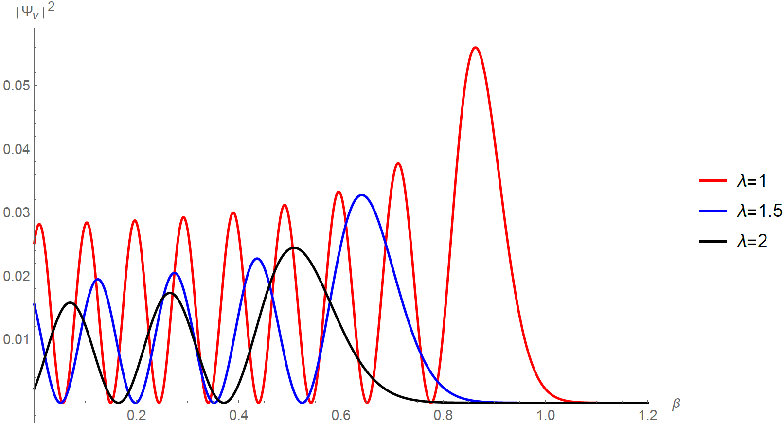
Figure 1: Absolute value squared of the wave functional $|\Psi_{\nu}|^{2}$ choosing $\nu=20i$ for $\lambda=1$ (red curve), $\lambda=1.5$ (blue curve) and $\lambda=2$ (black curve).

3 Hořava-Lifshitz gravity with GUP

Now that we have considered the WDW equation coming from the Kantowski-Sachs metric in HL gravity with the standard commutation relations, we now move on to study the changes made by considering the introduction of variables that obey a GUP. In particular we are going to use the relations inspired by [6], where a commutation relation that leads to a nonzero minimum uncertainty in the position variable is considered and that was used in [21] in the context of the WDW equation in GR. To be more precise we consider that the variables in minisuperspace obey the commutation relation

$$[q_{i},p_{j}]=i\delta_{ij}\left(1+\gamma^{2}p^{2}\right),$$ (15)

where $q_{1}=\Omega$, $q_{2}=\beta$, $p_{1}=P_{\Omega}$, $p_{\beta}=P_{\beta}$, $\gamma$ is a small parameter with units of inverse momentum and $p^{2}=p^{k}p_{k}$ is computed using the metric in superspace. We also introduce coordinates $q^{\prime}_{i}$ that obey the usual commutation relations, that is $[q^{\prime}_{i},p_{j}]=i\delta_{ij}$. In position space both sets of coordinates can be related as

$$q_{i}=q^{\prime}_{i}\left(1+\gamma^{2}p^{2}\right).$$ (16)

We can also choose the following representation for the momentum operators

$$P_{\Omega}=-i\frac{\partial}{\partial\Omega^{\prime}},\hskip 28.45274ptP_{\beta}=-i\frac{\partial}{\partial\beta^{\prime}}.$$ (17)

We also note from (10) that in this case

$$p^{2}=(2\lambda-1)P^{2}_{\beta}-2(\lambda-1)P_{\beta}P_{\Omega}+\frac{1}{2}(\lambda-3)P^{2}_{\Omega}.$$ (18)

In order to obtain a WDW equation with this setup we have to rewrite each term in equation (7) in terms of the prime coordinates. To be able to rewrite all the exponential terms we are going to use repeatedly the Zassenhaus formula which states the following

$$e^{A+B}=e^{A}e^{B}e^{-\frac{1}{2}[A,B]}e^{\frac{1}{6}\left([A,[A,B]]+2[B,[A,B]]\right)}\cdots$$ (19)

where $\cdots$ denotes terms with commutators involving more than 3 operators.

To begin with we will consider the first term contributing to the potential in (10), using (16) we can write it as

$$\exp[-2\sqrt{3}\Omega]=\exp\left[-2\sqrt{3}\Omega^{\prime}-2\sqrt{3}\gamma^{2}\Omega^{\prime}p^{2}\right].$$ (20)

Therefore, using the Zassenhaus formula (19) with $A=-2\sqrt{3}\Omega^{\prime}$ and $B=-2\sqrt{3}\gamma^{2}\Omega^{\prime}p^{2}$ and considering only up to second order terms in $\gamma$ we obtain

$$\exp[-2\sqrt{3}\Omega]\simeq\exp\left[-2\sqrt{3}\left\{1-2\gamma^{2}(\lambda-3)\right\}\Omega^{\prime}\right]\exp\left[-2\sqrt{3}\gamma^{2}\Omega^{\prime}p^{2}\right]\\ \times\exp\left[-6i\gamma^{2}\Omega^{\prime}\left\{(\lambda-3)P_{\Omega}-2(\lambda-1)P_{\beta}\right\}\right].$$ (21)

Carrying out the same procedure we obtain for the remaining terms

$$\exp\left[2\sqrt{3}\beta\right]\simeq\exp\left[2\sqrt{3}\left\{1-4\gamma^{2}(2\lambda-1)\right\}\beta^{\prime}\right]\exp\left[2\sqrt{3}\gamma^{2}\beta^{\prime}p^{2}\right]\\ \times\exp\left[-12i\gamma^{2}\beta^{\prime}\left\{(2\lambda-1)P_{\beta}-(\lambda-1)P_{\Omega}\right\}\right],$$ (22)

$$\exp\left[-2\sqrt{3}(\beta+2\Omega)\right]\simeq\exp\left[-2\sqrt{3}(1+12\gamma^{2})(\beta^{\prime}+2\Omega^{\prime})\right]\exp\left[-2\sqrt{3}\gamma^{2}(\beta^{\prime}+2\Omega^{\prime})p^{2}\right]\\ \times\exp\left[-12i\gamma^{2}(\beta^{\prime}+2\Omega^{\prime})(P_{\beta}-2P_{\Omega})\right],$$ (23)

$$\exp\left[2\sqrt{3}(2\beta+\Omega)\right]\simeq\exp\left[2\sqrt{3}\left\{1-6\gamma^{2}(3\lambda-1)\right\}(2\beta^{\prime}+\Omega^{\prime})\right]\exp\left[2\sqrt{3}\gamma^{2}(2\beta^{\prime}+\Omega^{\prime})p^{2}\right]\\ \times\exp\left[-6i\gamma^{2}(3\lambda-1)(2\beta^{\prime}+\Omega^{\prime})(2P_{\beta}-P_{\Omega})\right].$$ (24)

Now that we have expressed all the factors in terms of prime coordinates we proceed to study its behaviour when they are applied to the wave functional. Let us study first the term in (21). First of all up to second order in $\gamma$ and momentum we obtain

$$e^{-2\sqrt{3}\Omega}\Psi(\Omega,\beta)\simeq\exp\left[-2\sqrt{3}\left\{1-2\gamma^{2}(\lambda-3)\right\}\Omega^{\prime}\right]\exp\left[-2\sqrt{3}\gamma^{2}\Omega^{\prime}p^{2}\right]\\ \times\exp\left[-6i\gamma^{2}\Omega^{\prime}\left\{(\lambda-3)P_{\Omega}-2(\lambda-1)P_{\beta}\right\}\right]\Psi(\Omega^{\prime},\beta^{\prime}),$$ (25)

Then, we have two options to study the result of applying the exponential terms with linear momenta to the wave functional. The first one is to note that up to second order in $\gamma$ we can write

$$\exp\left[-6i\gamma^{2}\Omega^{\prime}\left\{(\lambda-3)P_{\Omega}-2(\lambda-1)P_{\beta}\right\}\right]\\ =\exp\left[12i\gamma^{2}(\lambda-1)\Omega^{\prime}P_{\beta}\right]\exp\left[-6i\gamma^{2}(\lambda-3)\Omega^{\prime}P_{\Omega}\right],$$ (26)

and we note that by defining $\Omega^{\prime}=e^{y}$ and using (17) we have

$$\Omega^{\prime}P_{\Omega}=-i\frac{\partial}{\partial y}.$$ (27)

Consequently the last term in (26) acts as a translation operator for the variable $y$, that corresponds to a scaling of the variable $\Omega^{\prime}$. Thus we obtain

$$\exp\left[-6i\gamma^{2}(\lambda-3)\Omega^{\prime}P_{\Omega}\right]\Psi(\Omega^{\prime},\beta^{\prime})=\Psi(e^{-6\gamma^{2}(\lambda-3)}\Omega^{\prime},\beta^{\prime}).$$ (28)

Moreover, if we expand the exponential in the first term of (26) as a power series and keep it only up to second order in $\gamma$ we finally obtain for the first option

$$\exp\bigg{\{}-6i\gamma^{2}\Omega^{\prime}\left((\lambda-3)P_{\Omega}-2(\lambda-1)P_{\beta}\right)\bigg{\}}\Psi(\Omega^{\prime},\beta^{\prime})\\ \simeq\left[1+12i\gamma^{2}\Omega^{\prime}(\lambda-1)P_{\beta}\right]\Psi(e^{-6\gamma^{2}(\lambda-3)}\Omega^{\prime},\beta^{\prime}).$$ (29)

Therefore, substituting it back into (25) and expanding as well the second exponential in the same way we obtain

$$e^{-2\sqrt{3}\Omega}\Psi(\Omega,\beta)\simeq e^{-2\sqrt{3}[1-2\gamma^{2}(\lambda-3)]\Omega^{\prime}}\bigg{\{}1+12i\gamma^{2}\Omega^{\prime}(\lambda-1)P_{\beta}\\ -2\sqrt{3}\gamma^{2}\Omega^{\prime}p^{2}\bigg{\}}\Psi(e^{-6\gamma^{2}(\lambda-3)}\Omega^{\prime},\beta^{\prime}).$$ (30)

On the other hand, instead of interpreting the second term in (26) as an scaling on $\Omega^{\prime}$, as in (28), we could also expand the exponential and keep only up to second order in $\gamma$, therefore we have for the second option

$$e^{-2\sqrt{3}\Omega}\Psi(\Omega,\beta)\simeq\exp^{-2\sqrt{3}\big{[}1-2\gamma^{2}(\lambda-3)\big{]}\Omega^{\prime}}\bigg{\{}1-6i\gamma^{2}\Omega^{\prime}\big{[}(\lambda-3)P_{\Omega}-2(\lambda-1)P_{\beta}\big{]}\\ -2\sqrt{3}\gamma^{2}\Omega^{\prime}p^{2}\bigg{\}}\Psi(\Omega^{\prime},\beta^{\prime}).$$ (31)

We note that both options are equivalent at the level of approximation used, that is, up to second order in $\gamma$ and momenta. Therefore we can use each of the options when we find it more useful.

We also note that the arguments used to get (28) are applicable to any term that contains a factor of the form a product of a coordinate times its momentum within an exponential. Therefore any of the terms (22)-(24) have also two possible expansions similarly to (30) and (31), and we will use any of them when we find it more useful.

Now that we have explained the general way in which any of the terms contributing to the WDW equation (10) are expressed in terms of prime coordinates and how they act on the corresponding wave functional. Thus we obtain the general WDW equation that takes into account the new commutation relations (15). Taking in all cases the second option of the form (31) for simplicity we obtain the equation

$$\bigg{\{}\left[1+\gamma^{2}F(\Omega^{\prime},\beta^{\prime})\right]\left[(2\lambda-1)P^{2}_{\beta}-2(\lambda-1)P_{\beta}P_{\Omega}+\frac{1}{2}(\lambda-3)P^{2}_{\Omega}\right]\\ +i\gamma^{2}G(\Omega^{\prime},\beta^{\prime},P_{\Omega},P_{\beta})+\widetilde{V}(\Omega^{\prime},\beta^{\prime})\bigg{\}}\Psi(\Omega^{\prime},\beta^{\prime})=0,$$ (32)

where we have defined

$$F(\Omega^{\prime},\beta^{\prime})=48\sqrt{3}(3\lambda-1)\Omega^{\prime}e^{-2\sqrt{3}\left[1-2\gamma^{2}(\lambda-3)\right]\Omega^{\prime}}\\ -48\sqrt{3}(3\lambda-1)\Lambda(\beta^{\prime}+2\Omega^{\prime})e^{-2\sqrt{3}(1+12\gamma^{2})(\beta^{\prime}+2\Omega^{\prime})}\\ +24\sqrt{3}g_{r}(3\lambda-1)\beta^{\prime}e^{2\sqrt{3}\left[1-4\gamma^{2}(2\lambda-1)\right]\beta^{\prime}}\\ +24\sqrt{3}g_{s}(3\lambda-1)(2\beta^{\prime}+\Omega^{\prime})e^{2\sqrt{3}\left[1-6\gamma^{2}(3\lambda-1)\right](2\beta^{\prime}+\Omega^{\prime})},$$ (33)

$$G(\Omega^{\prime},\beta^{\prime},P_{\Omega},P_{\beta})=144(3\lambda-1)\Omega^{\prime}\left[(\lambda-3)P_{\Omega}-2(\lambda-1)P_{\beta}\right]e^{-2\sqrt{3}\left[1-2\gamma^{2}(\lambda-3)\right]\Omega^{\prime}}\\ -288(3\lambda-1)\Lambda(\beta^{\prime}+2\Omega^{\prime})(P_{\beta}-2P_{\Omega})e^{-2\sqrt{3}(1+12\gamma^{2})(\beta^{\prime}+2\Omega^{\prime})}\\ -144g_{r}(3\lambda-1)\beta^{\prime}\left[(2\lambda-1)P_{\beta}-(\lambda-1)P_{\Omega}\right]e^{2\sqrt{3}\left[1-4\gamma^{2}(2\lambda-1)\right]\beta^{\prime}}\\ -72g_{s}(3\lambda-1)^{2}(2\beta^{\prime}+\Omega^{\prime})(2P_{\beta}-P_{\Omega})e^{2\sqrt{3}\left[1-6\gamma^{2}(3\lambda-1)\right](2\beta^{\prime}+\Omega^{\prime})},$$ (34)

$$\widetilde{V}(\Omega^{\prime},\beta^{\prime})=-24(3\lambda-1)e^{-2\sqrt{3}\left[1-2\gamma^{2}(\lambda-3)\right]\Omega^{\prime}}+24(3\lambda-1)\Lambda e^{-2\sqrt{3}(1+12\gamma^{2})(\beta^{\prime}+2\Omega^{\prime})}\\ +12g_{r}(3\lambda-1)e^{2\sqrt{3}\left[1-4\gamma^{2}(2\lambda-1)\right]\beta^{\prime}}+12g_{s}(3\lambda-1)e^{2\sqrt{3}\left[1-6\gamma^{2}(3\lambda-1)\right](2\beta^{\prime}+\Omega^{\prime})}.$$ (35)

Of course this equation is very complicated to solve in general, therefore in the next section we will restrict ourselves to the limiting cases considered in Sec. 2 and look for analytical solutions.

4 Infrared and Ultraviolet limits

In this section we are going to consider limiting cases of the WDW equation obtained in the last section. We note that due of the expansions leading to the expressions (21)-(24) we have carried out the following changes regarding the exponential terms

• $e^{-2\sqrt{3}\Omega}\to e^{-2\sqrt{3}\left[1-2\gamma^{2}(\lambda-3)\right]\Omega^{\prime}}$

• $\Lambda e^{-2\sqrt{3}(\beta+2\Omega)}\to\Lambda e^{-2\sqrt{3}(1+12\gamma^{2})(\beta^{\prime}+2\Omega^{\prime})}$

• $g_{r}e^{2\sqrt{3}\beta}\to g_{r}e^{2\sqrt{3}\left[1-4\gamma^{2}(2\lambda-1)\right]\beta^{\prime}}$

• $g_{s}e^{2\sqrt{3}(2\beta+\Omega)}\to g_{s}e^{2\sqrt{3}\left[1-6\gamma^{2}(3\lambda-1)\right](2\beta+\Omega)}$.

Therefore, we need to be careful in order not to change the signs of the exponentials so the same terms that we have seen are contributing in each limiting case in Sec. 2 are not altered. Therefore, we seek that all the new factors in the exponentials are positive, that is we demand that

$$\frac{1}{\gamma^{2}}>\sup\left(6(3\lambda-1),4(2\lambda-1)\right)=\begin{cases}6(3\lambda-1),\hskip 14.22636pt\lambda>\frac{1}{5},\\ 4(2\lambda-1),\hskip 14.22636pt\lambda<\frac{1}{5},\end{cases}$$ (36)

which can be easily fulfilled because $\gamma$ is taken to be a very small parameter.

As it was precisely the case in Sec. 2, the IR limit is obtained when $t>>1$ and $\lambda\to 1$, that is, we look for the terms containing negative exponentials in the WDW equation. Therefore, taking a vanishing cosmological constant and a term of the first form (30) we obtain in this limit

$$\left[\left(1+96\sqrt{3}\gamma^{2}\Omega^{\prime}e^{-2\sqrt{3}(1+4\gamma^{2})\Omega^{\prime}}\right)\left(P^{2}_{\beta}-P^{2}_{\Omega}\right)-48e^{-2\sqrt{3}(1+4\gamma^{2})\Omega^{\prime}}\right]\Psi\left(e^{12\gamma^{2}}\Omega^{\prime},\beta^{\prime}\right)\simeq 0.$$ (37)

This result can be compared with the equation discussed in [21].

In the other extreme limit now that we have imposed the conditions (36), we know that the contributing terms are the $g_{r}$ and $g_{s}$ ones. However, we are going to consider just the case discussed in Sec. 2 that was shown to have an analytical solution in the previous case. Therefore we consider $g_{r}=2$ and $g_{s}=0$. Thus, using an expansion of the first form (25) for the $g_{r}$ term we obtain the WDW equation

$$\left\{\left[1+48\sqrt{3}(3\lambda-1)\gamma^{2}\beta^{\prime}e^{2\sqrt{3}\left[1-4\gamma^{2}(2\lambda-1)\right]\beta^{\prime}}\right]\left[(2\lambda-1)\frac{\partial^{2}}{\partial\beta^{\prime 2}}-2(\lambda-1)\frac{\partial}{\partial\beta^{\prime}}\frac{\partial}{\partial\Omega^{\prime}}\right.\right.\\ \left.\left.+\frac{\lambda-3}{2}\frac{\partial^{2}}{\partial\Omega^{\prime 2}}\right]-36(2\lambda-1)(\lambda-1)\mu^{2}\gamma^{2}\beta^{\prime}e^{2\sqrt{3}\left[1-4\gamma^{2}(2\lambda-1)\right]\beta^{\prime}}\frac{\partial}{\partial\Omega^{\prime}}\right.\\ \left.-3(2\lambda-1)\mu^{2}e^{2\sqrt{3}\left[1-4\gamma^{2}(2\lambda-1)\right]\beta^{\prime}}\right\}\Psi(\Omega^{\prime},e^{-12\gamma^{2}(2\lambda-1)}\beta^{\prime})\simeq 0.$$ (38)

Inspired by the solution (14) we propose a general ansatz of the form

$$\Psi\left(\Omega^{\prime},e^{-12\gamma^{2}(2\lambda-1)}\beta^{\prime}\right)=e^{\sqrt{3}\nu\Omega^{\prime}}\left[e^{\sqrt{3}\beta^{\prime}}\right]^{\frac{\lambda-1}{2\lambda-1}\nu}\chi(\beta^{\prime}).$$ (39)

Substituting back (39) into (38) we obtain that the $\chi(\beta^{\prime})$ function obeys the equation

$$\left[\frac{d^{2}}{d\beta^{\prime 2}}-V\right]\chi(\beta^{\prime})=0,$$ (40)

where we have defined the function

$$V=\frac{3\nu^{2}(3\lambda-1)}{2(2\lambda-1)^{2}}+\frac{1+12(\lambda-1)\sqrt{3}\nu\gamma^{2}\beta^{\prime}}{1+48\sqrt{3}(3\lambda-1)\gamma^{2}\beta^{\prime}e^{2\sqrt{3}\left[1-4\gamma^{2}(2\lambda-1)\right]\beta^{\prime}}}\frac{24(3\lambda-1)}{(2\lambda-1)}e^{2\sqrt{3}\left[1-4\gamma^{2}(2\lambda-1)\right]\beta^{\prime}}.$$ (41)

Since we are working in an UV limit, i.e., when $t=e^{-\sqrt{3}(\beta^{\prime}+\Omega^{\prime})}<<1$, we note that this limit can be achieved by considering $\beta^{\prime}>>1$. Therefore, we can approximate the denominator of (41) as

$$1+48\sqrt{3}(3\lambda-1)\gamma^{2}\beta^{\prime}e^{2\sqrt{3}\left[1-4\gamma^{2}(2\lambda-1)\right]\beta^{\prime}}\simeq 48\sqrt{3}(3\lambda-1)\gamma^{2}\beta^{\prime}e^{2\sqrt{3}\left[1-4\gamma^{2}(2\lambda-1)\right]\beta^{\prime}},$$ (42)

and then, we can approximate the $V$ function as

$$V^{UV}=V\bigg{\rvert}_{\beta^{\prime}>>1}=A_{\nu,\lambda}+\frac{B_{\gamma,\lambda}}{\beta^{\prime}},$$ (43)

where

$$A_{\nu,\lambda}=\frac{3\nu}{2\lambda-1}\left[\frac{\nu(3\lambda-1)}{2(2\lambda-1)}+2(\lambda-1)\right],\hskip 28.45274ptB_{\gamma,\lambda}=\frac{1}{2\sqrt{3}(2\lambda-1)\gamma^{2}}.$$ (44)

Then, using the approximated potential (43) into (40) we obtain that the general solution is of the form

$$\chi(\beta^{\prime})=CM_{\kappa,1/2}\left(2\sqrt{A_{\nu,\lambda}}\beta^{\prime}\right)+DW_{\kappa,1/2}\left(2\sqrt{A_{\nu,\lambda}}\beta^{\prime}\right),$$ (45)

where $C$ and $D$ are constants, $M_{k,m}(z)$ and $W_{k,m}(z)$ are the solutions of the Whittaker differential equation and

$$\kappa=-\frac{B_{\gamma,\lambda}}{2\sqrt{A_{\nu,\lambda}}}.$$ (46)

We note that contrary to the situation discussed in Sec. 2, in the present case there is no restriction that lead us to take values of $\nu$ purely imaginary. Therefore in this case we have the freedom to propose values of $\nu$ real, purely imaginary or even complex focusing only on obtaining a well defined behaviour for the wave functionals. However, as it is usual in quantum cosmological models, we are looking for oscillatory solutions which can be interpreted as Lorentzian geometries [41, 42, 43] and it can be proved [44, 45] that the Whittaker equation found for the function $\chi$ does not have oscillatory solutions if $A_{\nu,\lambda}$ is a positive real number and $B_{\gamma,\lambda}$ is also positive. This can be achieved if $\nu$ takes positive real values and $\lambda>1/2$ (which is the values of interest to us). Therefore, positive real numbers for $\nu$ will not be considered in the following. We note that in all cases the function $|W_{\kappa,1/2}|^{2}$ exhibits a monotonically decreasing behaviour and therefore we can consider in (45) only the $M$ function, therefore we obtain finally that the wave functional is given by

$$\Psi\left(\Omega^{\prime},e^{-12\gamma^{2}(2\lambda-1)}\beta^{\prime}\right)=Ce^{\sqrt{3}\nu\Omega^{\prime}}\left[e^{\sqrt{3}\beta^{\prime}}\right]^{\frac{\lambda-1}{2\lambda-1}\nu}M_{\kappa,1/2}\left(2\sqrt{A_{\nu,\lambda}}\beta^{\prime}\right).$$ (47)

However, the behaviour of the squared absolute value of this wave functional $|\Psi|^{2}$ with respect to $\beta^{\prime}$ is troublesome. In most cases it only acts as a monotonically increasing function which is not a behaviour we are interested in. Nonetheless, for some values of the parameters it is possible to obtain an oscillatory behaviour. For example for values of $\lambda>1$ it is possible to obtain a decreasing oscillatory behaviour if we choose $\nu$ as a negative real number (with $A_{\nu,\lambda}$ nonpositive) or a complex number with negative real part. In Figures 2 and 3 we show plots of the projection of $|\Psi|^{2}$ with respect to $\beta^{\prime}$ choosing $|Ce^{\sqrt{3}\nu\Omega^{\prime}}|^{2}=1$. In Figure 2 we choose $\lambda=1.5$ and $\nu=10i-1$, we show curves for three different values of $\gamma$. We note that as $\gamma$ increases, the absolute value squared of the wave functional decreases. In the other hand, in Figure 3 we also choose $\nu=10i-1$ and $\gamma=0.1$, however in this case we show curves for three different values of $\lambda$. We obtain also that as $\lambda$ increases, the absolute value squared of the wave functional decreases. We note however that in both cases we are limited to a small interval to vary both parameters $\gamma$ or $\lambda$, since if we change one of them too much without changing the other or $\nu$, the behaviour can be easily spoiled. We also note that the oscillatory behaviour is present at first but it is reduced as $\beta^{\prime}$ increases and eventually it behaves just as a monotonically decreasing function, thus the parameters must be chosen such that the region of oscillatory behaviour is in agreement with the region where the approximation (42) is valid. This also happens if $\nu$ is taken as a real negative number. Finally, in Figure 4 we show the absolute value squared of the complete wave functional choosing $|C|^{2}=1$, $\nu=10i-1$, $\lambda=1.5$ and $\gamma=0.1$. We see that the dependence on $\Omega^{\prime}$ is just a negative exponential as shown in (47).

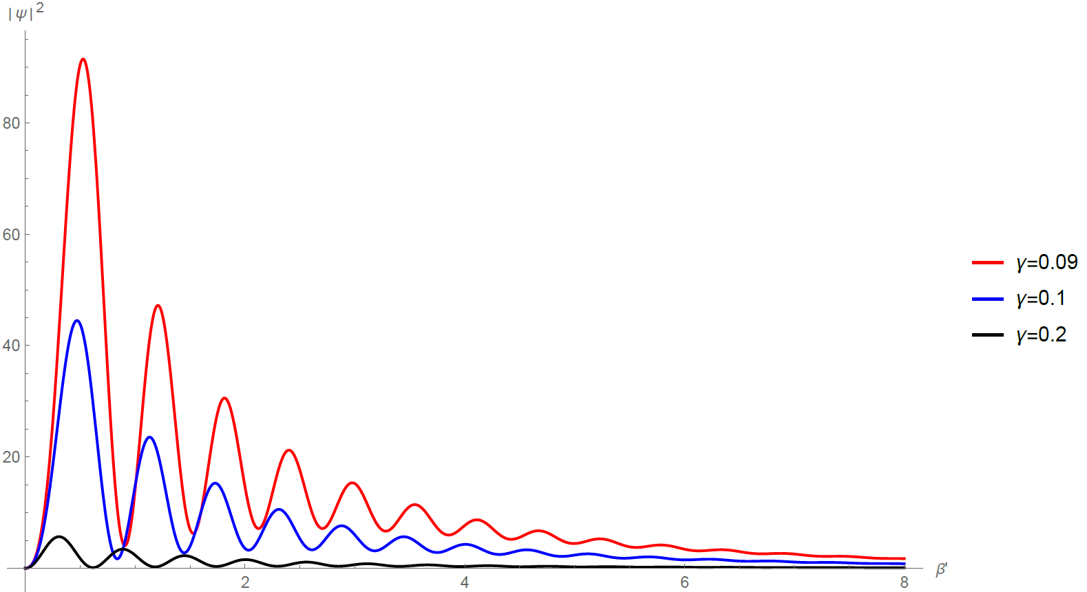
Figure 2: Projection of the absolute value squared of the wave functional $|\Psi|^{2}$ choosing $|Ce^{\sqrt{3}\nu\Omega^{\prime}}|^{2}=1$, $\lambda=1.5$ and $\nu=10i-1$ for $\gamma=0.09$ (red curve), $\gamma=0.1$ (blue curve) and $\gamma=0.2$ (black curve).

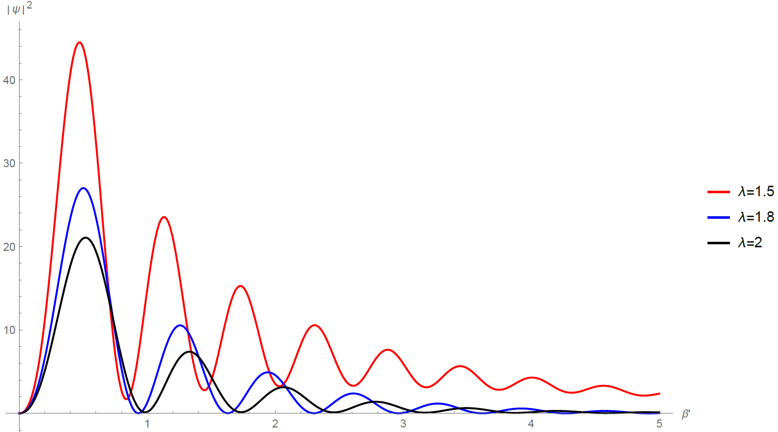
Figure 3: Projection of the absolute value squared of the wave functional $|\Psi|^{2}$ choosing $|Ce^{\sqrt{3}\nu\Omega^{\prime}}|^{2}=1$, $\gamma=0.1$ and $\nu=10i-1$ for $\lambda=1.5$ (red curve), $\lambda=1.8$ (blue curve) and $\lambda=2$ (black curve).

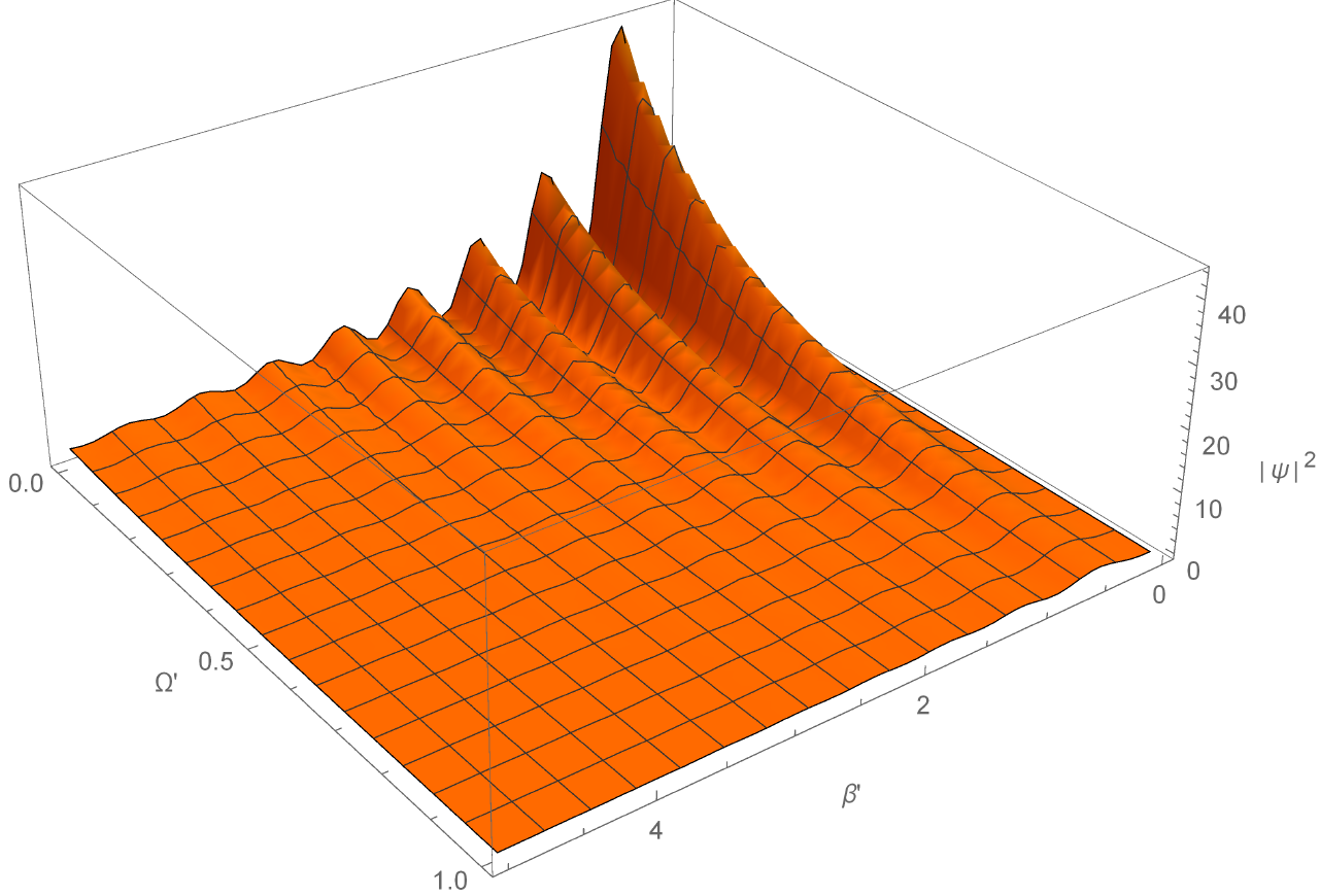
Figure 4: Absolute value squared of the wave functional $|\Psi|^{2}$ choosing $|C|^{2}=1$, $\lambda=1.5$, $\gamma=0.1$ and $\nu=10i-1$.

It can be appreciated from (44) that the case in which $\lambda=1$ is a particular one since in that case $A_{\nu,\lambda}$ only depends on $\nu^{2}$. For this particular case an oscillatory solution can also be found if we choose $\nu$ as a completely imaginary number, but in this case the oscillations do not decrease in height after a few peaks. In Figure 5 we show the plot of the projection of $|\Psi|^{2}$ with respect to $\beta^{\prime}$ choosing $|Ce^{\sqrt{3}\nu\Omega^{\prime}}|^{2}=1$ in this particular case. We take $\nu=5i$ and show curves for three different values of $\gamma$. In this case we also have the result found previously, that is, the absolute squared value of the wave functional increases inversely with $\gamma$.

From this analysis we can conclude that the form of the solution considering a GUP (39) has a similar form as the one obtained with the usual uncertainty relation (14) but the special function is modified from a Bessel function to a Whitakker function. This of course leads us to a different behaviour for the absolute value of the squared wave functional. For $\lambda>1$ we have in both cases a finite region of oscillatory behaviour starting from the origin at $\beta=0$ or $\beta^{\prime}=0$. However in the solution (14) this is achieved when $\nu$ is a purely imaginary number and the height of the oscillations increases until it reaches a maximum value whereas after considering a GUP the height of the oscillations have the opposite behaviour, that is they decrease until the oscillatory behaviour stops and it can be found when $\nu$ is a real negative number or a complex number with negative real part. We also note that in the GUP case we used a limit of $\beta^{\prime}>>1$ and therefore some of the region of oscillatory behaviour is not accessible. In both cases we obtain that as $\lambda$ increases the squared wave functional decreases. Finally, the $\lambda=1$ case is a special one in the GUP scenario where we obtain a oscillatory behaviour that does not decrease in height, whereas in the solution (14) this value of $\lambda$ is not special, it produces the same behaviour described earlier.

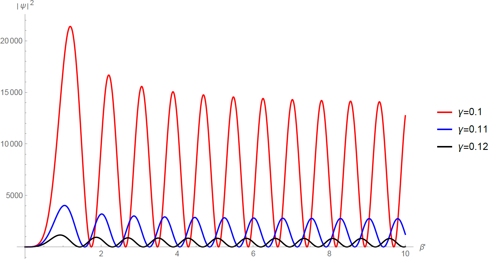
Figure 5: Projection of the absolute value squared of the wave functional $|\Psi|^{2}$ choosing $|Ce^{\sqrt{3}\nu\Omega^{\prime}}|^{2}=1$, $\lambda=1$ and $\nu=5i$ for $\gamma=0.1$ (red curve), $\gamma=0.11$ (blue curve) and $\gamma=0.12$ (black curve).

The $\boldsymbol{\gamma\to 0}$ limit
Before we end up let us discuss a subtle issue regarding the limit $\gamma\to 0$. If we take such limit in Eq. (38) it simplifies yielding (13) as expected. We also note that in this limit Eq. (40) gives the equation obeyed by the modified Bessel function of second order with the appropiate change of variables. Therefore in this limit the ansatz (39) gives smoothly the same solution (14) as expected. However, we note from (44) that in this limit $B_{\gamma,\lambda}$ is divergent and therefore we cannot obtain the solution in the standard case from the solutions found by considerind a GUP (47). This is because the ultraviolet approximation (42) considered in order to obtain analytic solutions is no longer valid if we take the $\gamma\to 0$ limit. Therefore, the region of validity of the solutions found in terms of the Wittaker functions depend not only on $\beta^{\prime}$ but also in $\gamma$ as well.

We may be tempted to look for analytic solutions that smoothly recover the solution (14) by expanding the denominator in the second term of (41) and keep only up to second order in the parameter $\gamma$. However, we note that in this case $\gamma$ is acompannied by a positive exponential term depending on $\beta^{\prime}$ and therefore it is not justified to keep only up to second order on $\gamma$ since in this case the whole term is not small in general. In fact, it can only be small for small values of $\beta^{\prime}$ which is the opposite of the UV limit considered. Therefore we believe it is more appropriate to use the UV approximation in the denominator and restrict ourselves to its corresponding region of validity.

5 Final Remarks

In the present article we have studied the Wheeler-DeWitt equation coming from a Kantowski-Sachs metric in Hořava-Lifshitz gravity with coordinates of minisuperspace that obey a GUP of the form proposed in [6] using the procedure presented originally in [21].

We first presented the WDW equation coming from the coordinates that obey the usual uncertainty relation and considered two limiting cases. In the IR limit the equation was reduced to the one found if one uses GR [21]. On the other hand, in the UV limit we were able to find the equation coming from HL gravity with the projectability condition and with detailed balance, but in this case it was found to be only an approximation of the theory without detailed balance after choosing specific values for the $g_{r}$ and $g_{s}$ constants. In both cases analytic solutions were found and the behaviour of the UV solution was presented in Figure 1. We found that the solutions describe a finite region of oscillatory behaviour with an increasing height until it reaches a maximum peak, then the oscillatory behaviour stops and it starts decreasing. We also found that as $\lambda$ increases the absolute value squared of the wave functional decreases.

We then moved on to study the WDW equation when the coordinates on minisuperspace obey a GUP. We used the general procedure to modify the WDW equation obtained previously by using the relations between both sets of coordinates and consider only terms up to second order in momentum as well as second order on the GUP parameter $\gamma$. Since all terms contain exponentials of the form a coordinate times its corresponding momentum, we found that there was two possible procedures to obtain the WDW equation depending on how we take this term when acting on the wave functional. They can be interpreted as terms that scale the coordinates in the wave functional as in [21], this interpretation was used when we studied the limiting cases and look for analytic solutions. However, they can also be interpreted as to contribute with terms of linear momenta without rescaling the coordinates on the wave functional, this form was useful to obtain the WDW equation in general.

Since the general WDW equation, which is valid in all cases, was found to be very difficult, we proceeded to study the limiting cases considered before. In the IR limit we found an equation that can be compared to the result obtained by using GR in [21]. In the UV limit we considered special values of $g_{r}$ and $g_{s}$ as we mentioned before. We showed that this limit could be achieved if we take $\beta^{\prime}>>1$ and therefore, we approximated the resulting equation. We then obtained an analytic solution of such equation in terms of special functions. We found that the general form of the solution was the same as the one encountered when the coordinates obey the standard uncertainty principle but now the special function was not a Bessel function of the second kind, it was instead a Whittaker function. We also noted that contrary to the standard case (without considering a GUP) in this case the parameter $\nu$ in the ansatz was not subject to a restriction and therefore we were free to choose $\nu$ as a real, purely imaginary or even a complex number. We only focused on the values that leaded us to a correct behaviour for the resulting wave functionals. We found that only one of the two possible Whittaker functions was able to produce oscillatory solutions but the dependence on the parameters $\nu$, $\gamma$ and $\lambda$ was found to be very restringing and the oscillatory behaviour is not present for any arbitrary values. It was also found that this behaviour was encountered only when $\nu$ was not allowed to be a positive real number. For $\lambda>1$ plots of the squared value of the wave functional $|\Psi|^{2}$ were presented in Figures 2, 3 and 4. We noted that the oscillatory behaviour is strong at first but then it decreases until it disappears, therefore it is necessary to look for an interval where the oscillatory behaviour and the approximation used are both valid. The peaks of the oscillations were found to decrease in height contrary to the behaviour found for the case without considering a GUP. We also showed that the value of $|\Psi|^{2}$ decreases if $\gamma$ or $\lambda$ was increased. The case $\lambda=1$ was found to be an special one, for this case an oscillatory behaviour could also be found and we presented a plot of it in Figure 5, however in this case the height of the oscillations does not decrease after a few peaks. In this case it was also shown that $|\Psi|^{2}$ decreases as $\gamma$ increases. Contrary to the standard scenario without a GUP where this case is not special and the behaviour is the same as for any other value of $\lambda$.

Finally, it would be interesting to consider a noncommutative deformation of the general WDW equation (10) found in this article. It is well known that the WDW equation (11) in GR, can be noncommutatively deformed in its Heisenberg algebra through a parameter $\theta$ [46]. This noncommutative deformation is also relevant at high energies and this represents another UV effect that should be taken into account since it is also related to the existence of a minimal length. Some solutions of the noncommutative deformation of (11) are known [46]. Thus they would be useful to find new solutions to the noncommutative deformation of the general WDW equation (10) similar to the procedure carried out in the present paper. Some of this work is in progress and will be reported elsewhere.

Acknowledgments

It is a pleasure to thank Prof. O. Obregón for comments on the manuscript. D. Mata-Pacheco would also like to thank CONACyT for a grant.

References

- [1] D. J. Gross, P. F. Mende, “String theory beyond the Planck scale,” Nucl. Phys. B 303 (1988), 407-454 doi:10.1016/0550-3213(88)90390-2.
- [2] D. Amati, M. Ciafaloni, G. Veneziano, “Can spacetime be probed below the string size?,” Phys. Lett. B 216, (1989), 41-47 doi:10.1016/0370-2693(89)91366-X.
- [3] M. Maggiore, “A Generalized uncertainty principle in quantum gravity,” Phys. Lett. B 304, 65-69 (1993) doi:10.1016/0370-2693(93)91401-8 [arXiv:hep-th/9301067 [hep-th]].
- [4] F. Scardigli, “Generalized uncertainty principle in quantum gravity from micro - black hole Gedanken experiment,” Phys. Lett. B 452, 39-44 (1999) doi:10.1016/S0370-2693(99)00167-7 [arXiv:hep-th/9904025 [hep-th]].
- [5] L. J. Garay, “Quantum gravity and minimum length,” Int. J. Mod. Phys. A 10, 145-166 (1995) doi:10.1142/S0217751X95000085 [arXiv:gr-qc/9403008 [gr-qc]].
- [6] A. Kempf, G. Mangano and R. B. Mann, “Hilbert space representation of the minimal length uncertainty relation,” Phys. Rev. D 52, 1108-1118 (1995) doi:10.1103/PhysRevD.52.1108 [arXiv:hep-th/9412167 [hep-th]].
- [7] M. A. Anacleto, F. A. Brito and E. Passos, “Quantum-corrected self-dual black hole entropy in tunneling formalism with GUP,” Phys. Lett. B 749, 181-186 (2015) doi:10.1016/j.physletb.2015.07.072 [arXiv:1504.06295 [hep-th]].
- [8] M. A. Anacleto, D. Bazeia, F. A. Brito and J. C. Mota-Silva, “Quantum-corrected two-dimensional Horava-Lifshitz black hole entropy,” Adv. High Energy Phys. 2016, 8465759 (2016) doi:10.1155/2016/8465759 [arXiv:1512.07886 [hep-th]].
- [9] F. Scardigli and R. Casadio, “Uncertainty relations and precession of perihelion,” J. Phys. Conf. Ser. 701, no.1, 012016 (2016) doi:10.1088/1742-6596/701/1/012016
- [10] F. Scardigli, G. Lambiase and E. Vagenas, “GUP parameter from quantum corrections to the Newtonian potential,” Phys. Lett. B 767, 242-246 (2017) doi:10.1016/j.physletb.2017.01.054 [arXiv:1611.01469 [hep-th]].
- [11] G. Lambiase and F. Scardigli, “Lorentz violation and generalized uncertainty principle,” Phys. Rev. D 97, no.7, 075003 (2018) doi:10.1103/PhysRevD.97.075003 [arXiv:1709.00637 [hep-th]].
- [12] E. C. Vagenas, L. Alasfar, S. M. Alsaleh and A. F. Ali, “The GUP and quantum Raychaudhuri equation,” Nucl. Phys. B 931, 72-78 (2018) doi:10.1016/j.nuclphysb.2018.04.004 [arXiv:1706.06502 [hep-th]].
- [13] P. Bosso, “Generalized Uncertainty Principle and Quantum Gravity Phenomenology,” [arXiv:1709.04947 [gr-qc]].
- [14] N. Demir and E. C. Vagenas, “Effect of the GUP on the Entropy, Speed of Sound, and Bulk to Shear Viscosity Ratio of an ideal QGP,” Nucl. Phys. B 933, 340-348 (2018) doi:10.1016/j.nuclphysb.2018.06.020 [arXiv:1806.09456 [hep-th]].
- [15] P. Bosso, S. Das and R. B. Mann, “Potential tests of the Generalized Uncertainty Principle in the advanced LIGO experiment,” Phys. Lett. B 785, 498-505 (2018) doi:10.1016/j.physletb.2018.08.061 [arXiv:1804.03620 [gr-qc]].
- [16] Z. Y. Fu and H. L. Li, “The effect of GUP on thermodynamic phase transition of Rutz-Schwarzschild black hole,” Nucl. Phys. B 969, 115475 (2021) doi:10.1016/j.nuclphysb.2021.115475
- [17] P. A. Bushev, J. Bourhill, M. Goryachev, N. Kukharchyk, E. Ivanov, S. Galliou, M. E. Tobar and S. Danilishin, “Testing the generalized uncertainty principle with macroscopic mechanical oscillators and pendulums,” Phys. Rev. D 100, no.6, 066020 (2019) doi:10.1103/PhysRevD.100.066020 [arXiv:1903.03346 [quant-ph]].
- [18] R. L. Arnowitt, S. Deser and C. W. Misner, “The Dynamics of general relativity,” Gen. Rel. Grav. 40, 1997-2027 (2008) doi:10.1007/s10714-008-0661-1 [arXiv:gr-qc/0405109 [gr-qc]].
- [19] J.A. Wheeler, “Superspace and the nature of quantum geometrodynamics,” pp 615-724 of Topics in Nonlinear Physics, (ed) N.J. Zabusky, Springer-Verlag NY, Inc., 1968. (1969).
- [20] B.S. DeWitt,“Quantum theory of gravity I, The canonical theory,” Phys. Rev. 160 (5) (1967) 1113.
- [21] P. Bosso and O. Obregón, “Minimal length effects on quantum cosmology and quantum black hole models,” Class. Quant. Grav. 37 (2020) no.4, 045003 doi:10.1088/1361-6382/ab6038 [arXiv:1904.06343 [gr-qc]].
- [22] H. García-Compeán, O. Obregón and C. Ramírez, “Topics in Supersymmetric and Noncommutative Quantum Cosmology,” Universe 7, no.11, 434 (2021) doi:10.3390/universe7110434
- [23] G. Barca, E. Giovannetti and G. Montani, “Comparison of the Semiclassical and Quantum Dynamics of the Bianchi I Cosmology in the Polymer and GUP Extended Paradigms,” [arXiv:2112.08905 [gr-qc]].
- [24] P. Hoava, “Quantum Gravity at a Lifshitz Point,” Phys. Rev. D 79, 084008 (2009) doi:10.1103/PhysRevD.79.084008 [arXiv:0901.3775 [hep-th]].
- [25] S. Weinfurtner, T. P. Sotiriou and M. Visser, “Projectable Hoava-Lifshitz gravity in a nutshell,” J. Phys. Conf. Ser. 222, 012054 (2010) doi:10.1088/1742-6596/222/1/012054 [arXiv:1002.0308 [gr-qc]].
- [26] T. P. Sotiriou, “Hoava-Lifshitz gravity: a status report,” J. Phys. Conf. Ser. 283, 012034 (2011) doi:10.1088/1742-6596/283/1/012034 [arXiv:1010.3218 [hep-th]].
- [27] A. Wang, “Hoava gravity at a Lifshitz point: A progress report,” Int. J. Mod. Phys. D 26, no. 07, 1730014 (2017) doi:10.1142/S0218271817300142 [arXiv:1701.06087 [gr-qc]].
- [28] S. Mukohyama, “Hoava-Lifshitz Cosmology: A Review,” Class. Quant. Grav. 27, 223101 (2010) doi:10.1088/0264-9381/27/22/223101 [arXiv:1007.5199 [hep-th]].
- [29] O. Bertolami and C. A. D. Zarro, “Hořava-Lifshitz Quantum Cosmology,” Phys. Rev. D 84 (2011), 044042 doi:10.1103/PhysRevD.84.044042 [arXiv:1106.0126 [hep-th]].
- [30] T. Christodoulakis and N. Dimakis, “Classical and Quantum Bianchi Type III vacuum Hoava-Lifshitz Cosmology,” J. Geom. Phys. 62 (2012), 2401-2413 doi:10.1016/j.geomphys.2012.09.005 [arXiv:1112.0903 [gr-qc]].
- [31] J. P. M. Pitelli and A. Saa, “Quantum Singularities in Hoava-Lifshitz Cosmology,” Phys. Rev. D 86 (2012), 063506 doi:10.1103/PhysRevD.86.063506 [arXiv:1204.4924 [gr-qc]].
- [32] B. Vakili and V. Kord, “Classical and quantum Hořava-Lifshitz cosmology in a minisuperspace perspective,” Gen. Rel. Grav. 45 (2013), 1313-1331 doi:10.1007/s10714-013-1527-8 [arXiv:1301.0809 [gr-qc]].
- [33] O. Obregon and J. A. Preciado, “Quantum cosmology in Hořava-Lifshitz gravity,” Phys. Rev. D 86 (2012), 063502 doi:10.1103/PhysRevD.86.063502 [arXiv:1305.6950 [gr-qc]].
- [34] D. Benedetti and J. Henson, “Spacetime condensation in (2+1)-dimensional CDT from a Hořava–Lifshitz minisuperspace model,” Class. Quant. Grav. 32 (2015) no.21, 215007 doi:10.1088/0264-9381/32/21/215007 [arXiv:1410.0845 [gr-qc]].
- [35] R. Cordero, H. García-Compeán and F. J. Turrubiates, “A phase space description of the FLRW quantum cosmology in Hořava–Lifshitz type gravity,” Gen. Rel. Grav. 51 (2019) no.10, 138 doi:10.1007/s10714-019-2627-x [arXiv:1711.04933 [gr-qc]].
- [36] Y. S. Myung, “Generalized uncertainty principle and Hořava-Lifshitz gravity,” Phys. Lett. B 679, 491-498 (2009) doi:10.1016/j.physletb.2009.08.030 [arXiv:0907.5256 [hep-th]].
- [37] Y. S. Myung, “Generalized uncertainty principle, quantum gravity and Hořava-Lifshitz gravity,” Phys. Lett. B 681, 81-84 (2009) doi:10.1016/j.physletb.2009.09.062 [arXiv:0909.2075 [hep-th]].
- [38] T. P. Sotiriou, M. Visser and S. Weinfurtner, “Phenomenologically viable Lorentz-violating quantum gravity,” Phys. Rev. Lett. 102 (2009), 251601 doi:10.1103/PhysRevLett.102.251601 [arXiv:0904.4464 [hep-th]].
- [39] T. P. Sotiriou, M. Visser and S. Weinfurtner, “Quantum gravity without Lorentz invariance,” JHEP 10 (2009), 033 doi:10.1088/1126-6708/2009/10/033 [arXiv:0905.2798 [hep-th]].
- [40] C. W. Misner, “Minisuperspace,” in J.A. Wheeler, editor, Magic Without Magic John Archibald Wheeler, A collection in honor of his 60th birthday, pages 441-473 (1972).
- [41] S.W. Hawking, “The quantum state of the universe,” Nuclear Physics B 239 257-276 (1984), doi:10.1016/0550-3213(84)90093-2.
- [42] S. Wada, “Quantum Classical Correspondence in Wave Functions of the Universe,” Prog. Theor. Phys. 75, 1365 (1986) doi:10.1143/PTP.75.1365.
- [43] J. J. Halliwell, “Introductory Lectures on Quantum Cosmology,” edited by S. Coleman, J. B. Hartle, T. Piran and S. Weinberg, Proceedings of the Jerusalem Winter School on Quantum Cosmology and Baby Universes, World Scientific, Singapore (1991) [arXiv:0909.2566 [gr-qc]].
- [44] Q.D. Katatbeh, D.M. Christodoulou and J. Graham-Eagle, “The intervals of oscillations in the solutions of the radial Schrödinger differential equation,” Adv Differ Equ 2016, 47 (2016). doi:10.1186/s13662-016-0777-7.
- [45] E. Hille, “Non-oscillation theorems,” Trans. Amer. Math. Soc. 64 234 (1948).
- [46] H. Garcia-Compean, O. Obregon and C. Ramirez, “Noncommutative quantum cosmology,” Phys. Rev. Lett. 88, 161301 (2002) doi:10.1103/PhysRevLett.88.161301 [arXiv:hep-th/0107250 [hep-th]].