The Cascading Metric Tree

Abstract

This paper presents the Cascaded Metric Tree (CMT) for efficient satisfaction of metric search queries over a dataset of $N$ objects. It provides extra information that permits query algorithms to exploit all distance calculations performed along each path in the tree for pruning purposes. In addition to improving standard metric range (ball) query algorithms, we present a new algorithm for exploiting the CMT cascaded information to achieve near-optimal performance for $k$-nearest neighbor (kNN) queries. We demonstrate the performance advantage of CMT over classical metric search structures on synthetic datasets of up to 10 million objects and on the $564K$ Swiss-Prot protein sequence dataset containing over $200$ million amino acids. As a supplement to the paper, we provide reference implementations of the empirically-examined algorithms to encourage improvements and further applications of CMT to practical scientific and engineering problems.

1 Introduction

In this paper we examine new methods, as well as combinations of known methods, for augmenting metric search structures to provide a level of performance necessary for practical applications, e.g., involving large-scale protein and genomic sequence datasets. Our first contribution is the use of metric cascading, in the form of a cascaded metric tree (CMT) to permit every distance calculation performed along a path in a tree to provide an additional pruning test at every subsequent node along that path. In other words, if $P$ distance calculations have been performed along the path from the root node to a given node, then $O(P)$ fast independent scalar-inequality tests (i.e., not requiring computationally-expensive metric distance calculations) are available for pruning the search at that node.

We formally define a general family of cascaded metric tree structures for which the number of distance calculations per node is parameterized. However, our goal in this paper is to define a search structure and associated query algorithms that maximally exploit information from each distance calculation such that near-optimal performance can be expected without need for application-specific tuning. To this end, our tests only examine the most basic form with no parametric tuning of any kind.

2 Background

Perhaps the simplest generalization of the familiar 1d (scalar) balanced binary search tree (BST) to accommodate general metric search queries can be constructed by choosing one of the $n$ objects in a dataset and computing the distance (radius) from it to the remaining objects, with the object and the median distance stored at the root node. Applying this process recursively such that objects less than the median radius at a given node form the left subtree, and the remainder form the right subtree, yields a balanced metric binary search tree (MBST) such that the path to a given object is uniquely determined by a sequence of distance calculations starting at the root node. For example, if the distance between a given query object $s$ and the object $r$ stored at the root node is less than the radius stored at the node then $s$ must be in the left subtree, otherwise it must be in the right subtree. This provides a recursive search algorithm that is guaranteed to find $s$, or determine that object $s$ is not in the tree, using only $O(\log(N))$ distance calculations

Generalization of the MBST search algorithm to satisfy queries asking for all objects within a given distance from a query object, referred to as a metric range or ball query, are directly analogous to the satisfying of interval range queries in a BST where both subtrees of a node must be searched if the query range spans the partitioning value. In the case of the simple MBST, a metric range query can only prune a subtree from the search process when the metric ball determined by the object and radius at a given node does not intersect the query volume (ball). This requires only the calculation of the distance between the query object and the object at the node, followed by a triangle inequality test involving their respective radii. Thus, the triangle inequality property of metric distances is absolutely necessary for correctness of the algorithm when pruning is applied

As described thus far, the simple MBST only permits left subtrees to be pruned because there is no available bound on the spatial extent of objects in the right subtree. If in addition to the median, however, information defining the minimum-volume bounding ball is also stored at each node then an additional criterion for pruning will be available at each node during the search process. Unfortunately, this bounding ball cannot necessarily be made tight except in the case of vector spaces (which permit arithmetic operations to be performed on objects, e.g., to create a new object as the mean of two other objects) because there is no way in general to construct a virtual “spatial centroid” object in the general case of black-box distance functions and objects. However, it is possible to identify an object for which the maximum radius to any other object is minimized, but this incurs the cost of a potentially quadratic number of distance calculations during the tree construction process.

Clearly there are many degrees of freedom available during the tree construction process that can be tailored to potentially improve MBST query performance, (i.e., to reduce the average number of distance calculations per query) based on the characteristics of datasets that are deemed typical for a particular application. For example, the strict binary structure can be relaxed to a $b$-ary tree with branching-value $b$ determined empirically based on tests over representative datasets for a given application. Unfortunately, too many degrees of freedom can mask the fact that the search algorithm is suboptimal in its sensitivity to application-specific variables. Ideally, there would exist a data structure that provides consistent near-optimal performance such that minimal improvement can be expected from additional heuristic application-specific tuning. In other words, search structures and/or algorithms with few or no tunable parameters are likely to exhibit more robust practical performance than those for which good performance demands extensive tuning of many parameters.

3 Metric Search

A function $d(x,y)$ defines a metric distance on the set $S$ if for elements $x,y,z$ of $S$ if the properties in Table I hold.

TABLE I: Metric Properties $\forall\,x,y,z\in S$

$d(x,y)\geq 0$	non-negativityx
$d(x,y)=d(y,x)$	symmetry
$x=y\Rightarrow d(x,y)=0$	identity
$d(x,z)\leq d(x,y)+d(y,z)$	triangle inequality

Given a query object $q$, a search radius $r$, and a set $S$ of objects, a metric range query $R(q,r)$ over $S$ reports all objects in $S$ within distance $r$ of the object $q$. An exhaustive (brute force) search can satisfy the query by performing $|S|$ distance functions, but this may not be practical when $S$ is very large or when the relevant distance function $d(x,y)$ is computationally expensive to evaluate. However, the metric triangle inequality property offers a means for potentially reducing the number of distance calculations needed to satisfy such queries. For example, consider object $p\in S$ and $C\equiv\{S\setminus p\}$. Also assume that the nearest and farthest objects in $C$ from $p$ are at known distances $d(p,p_{n})$ and $d(p,p_{f})$, respectively. Given these conditions there exist queries $R(q,r)$ for which the performing of only one additional distance calculation $d(p,q)$ establishes that none of the objects in $C$ satisfy the query. For example, in the case when the query object $q$ is “far” from $p$ in the sense that it is farther from $p$ than any object in $S$, i.e, $d(q,p)>d(p,p_{f})$, then $d(q,p)>d(p,p_{f})+r$ implies $d(q,x)>r,\>\forall\,x\,\in\{C\}$:

Proof.

Let $d(q,p)-d(p,p_{f})>r$, so

$$d(q,x)\!+\!d(x,p)\!-\!d(p,p_{f})>r~{}\text{({triangle inequality})}$$

$$d(q,x)>r+[d(p,p_{f})-d(x,p)]$$

$$d(q,x)>r~{}~{}~{}~{}\text{({since $d(p,p_{f})\!-\!d(x,p)$ is positive})}$$

An analogous result holds for the case of a “near” query object, i.e., $d(q,p)<d(p,p_{n})$, when $d(q,p)>d(p,p_{n})-r$. It is convenient to view $d(p,p_{n})$ and $d(p,p_{f})$ as defining a distance interval $\mbox{DI}(p,C)\equiv[d(p,p_{n}),d(p,p_{f})]$ that bounds the distances from $p$ to the objects in $C$ and which may permit an immediate determination (via the triangle inequality) that the query ball cannot contain any objects in $C$. In other words, either of two simple inequality tests may establish that further searching is unnecessary. Various such inequalities have been examined in the literature and provide the standard means for exploiting metric assumptions for pruning searches of objects in large datasets.

The limitation of conventional metric search trees during the query process is that information obtained from the computation of a distance calculation between the query object and an object stored at a given node is only exploited for pruning purposes at that node. In the following section we describe a means for augmenting the search tree with additional information so that the pruning step at the current node can exploit all previous distance calculations performed along the path from the root to the current node.

3.1 Cascaded Metric Trees

Consider a dataset that is recursively decomposed into a metric search tree with one or more objects stored at each node. Purely for convenience of exposition we will assume a balanced binary tree with a single object stored at each node. We refer to the structure as a metric search structure because it is further assumed that any search algorithm must traverse the tree based on information obtained from black-box metric distance calculations involving objects stored along the sequence of visited nodes. Ideally, this information will permit the search space (i.e., the amount of the tree that must be traversed) to be significantly reduced so that the total number of performed distance calculations does not greatly exceed the number of objects that are found to satisfy the query.

Figure 1: In addition to an object, each CMT node contains distances between its object and all ancestor objects. (These distances are pre-computed during construction of the tree.) Because the query object has already computed distances between itself and the ancestor objects of the current node at depth $d$, an extra $d$ triangle-inequality tests can be performed without need for any extra distance calculations.

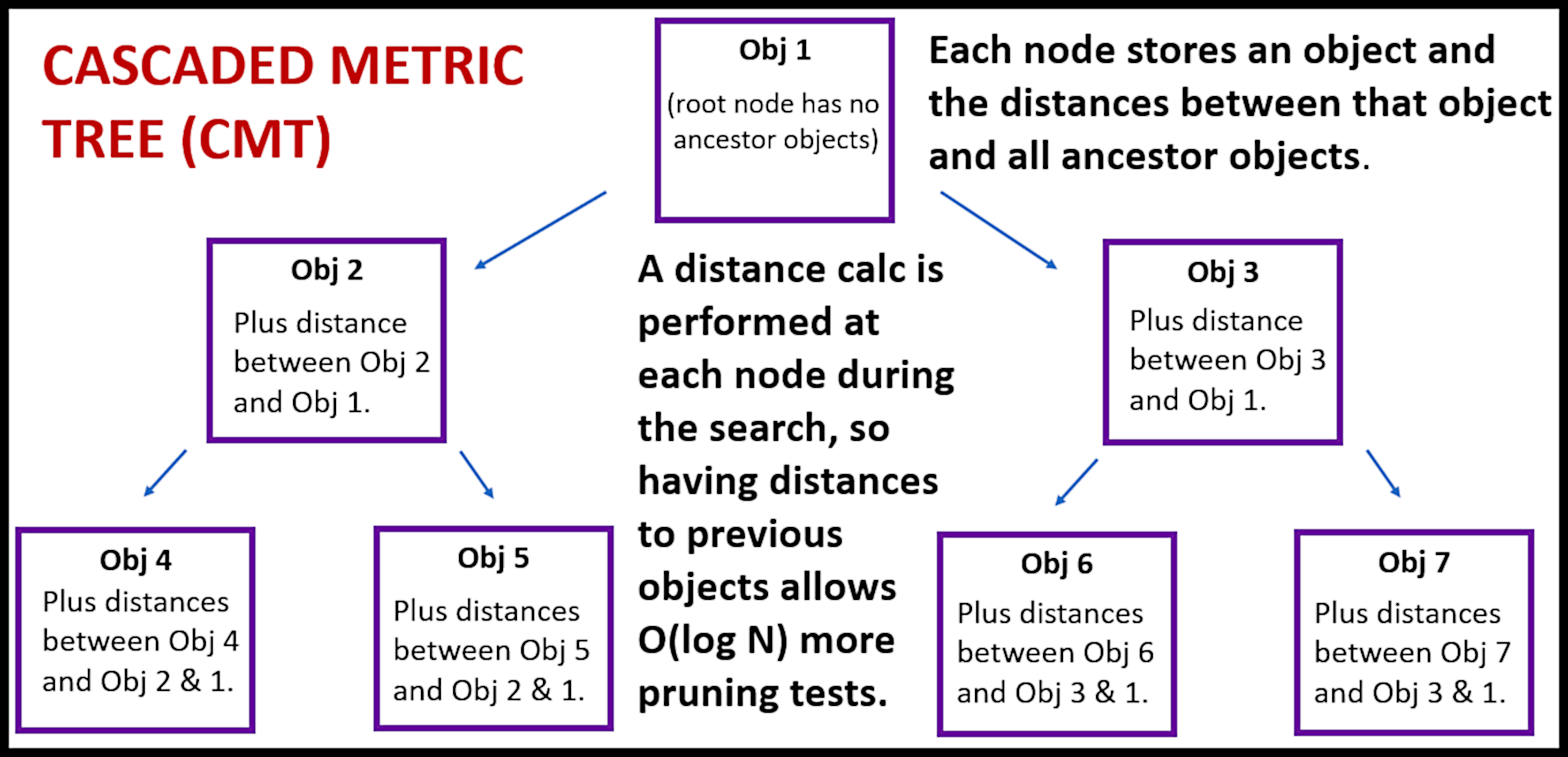
The principal feature of the cascaded metric tree (CMT) is that each node contains not only an object, but also stores the distance between that object and each object along the path from that node to the root of the tree (see Fig. 1). Because a distance calculation must have been performed between the query object and the ancestor objects visited along the path to the current node, all the information necessary to perform triangle-inequality pruning tests with respect those ancestor objects is available with no need for additional distance calculations. In other words, the number of “free” pruning tests at each node increases linearly with depth. More fundamentally, each distance calculation performed at a node during the search process is exploited in a pruning test at each subsequent node along that path in the tree, as opposed to a single pruning test at the current node.

Importantly, the CMT construction algorithm performs only $O(N\log N)$ total distance calculations, which is the same as that required for conventional linear-space metric search trees, despite the fact that CMT stores $O(\log N)$ ancestral distances at each node. This is possible because the CMT construction process is able to exploit cascaded distance information in a manner that is analogous to the search process.

To formalize the specification of the tree and search algorithms, we define the following notation for information defined for or maintained by the query algorithm:

• $q$ is the query object.

• $r\geq 0$ is the query radius. A value of $\infty$ may be implicitly or explicitly defined for the case in which no bound is placed on the size of the query radius.

• $k\geq 1$ is an integer limit on the size of the returned query set of nearest objects. A value of $\infty$ (or sufficiently large number greater than or equal to the size of the dataset) may be implicitly or explicitly defined for the case in which no limit is placed on the number of objects that may be returned.

• depth is the number of levels the current node is from the root. Thus, depth - 1 is the depth of the parent node, depth - 2 is the grandparent node, and the ancestor at level depth is the root node of the overall tree. The value of depth is dynamically maintained during the search/traversal process and thus is not a query parameter.

• dist[j] is the distance from $q$ to the $j$th ancestor of the current node $1\leq j<$ depth. This indexed list/vector is dynamically maintained during the search/traversal process and thus is not a query parameter.

And we define the following notation for information maintained at each CMT node:

• near[i] and far[i] provide near and far distance interval information with respect to the $i$th ancestor of the node. For example, near[1] is the distance of the object in the subtree rooted at the current node (which includes $p$) that is nearest to the node-object in the parent, and far[1] is analogously defined with respect to the farthest object in the subtree from the parent object. More generally, distance interval information with respect to the $i$th ancestor of the current node is similarly available for each index $1\leq i<$ depth. The values near[0] and far[0] provide the near and far distances to objects in the subtree beneath the current node, i.e., excluding the object $p$ at the current node.

• count provides the number of objects in the subtree of the current node. This is necessary to satisfy counting queries, which ask for the number of objects that satisfy a given query without actually retrieving those objects. More specifically, if the query volume completely contains the bounding volume of objects in the subtree of a given node (which can be determined from $p$ and far[0]), then the number of satisfying objects is immediately given by count without need to traverse the subtree. This permits counting queries to be satisfied with complexity sublinear in the number of objects that satisfy the query, e.g., $O(1)$ if the query volume is sufficiently large to enclose all objects in the tree.

• left and right are the left and right child nodes (subtrees) of the current node.

If the query interval/ball fails to intersect the distance interval/annulus for any ancestor $i$ then the entire subtree (including the node-object $p$) can be pruned from further consideration. This provides $O(\log N)$ separate pruning tests, each of which may immediately terminate search of the current subtree. More specifically, the number of pruning tests increases from $O(1)$ at the root node to $O(\mbox{\em height})$ at leaf nodes, which is $O(\log N)$ if the tree is balanced.

TABLE II: Information Relating to the Current Query

$q$x	The query object: goal is to find the $k$-nearest
	objects within distance $r$ of $q$.
$r$	The maximum allowed radius (distance) from the
	query object $q$.
$k$	The maximum allowed number of objects nearest
	to $q$ to be returned.
	(Below is information maintained during
	execution of each query)
depth	The number of levels the current node is
	from the root.
dist[j]	The distance from $q$ to the node-object
	of the $j$th ancestor of the current node.

TABLE III: Information Stored at Each Node of the CMT

$p$x	The node-object, i.e., the object stored at
	the node.
near[i],x	The min and max distances from the $i$th
far[i]	ancestor object to the objects in the subtree.
	(Index $0$ refers to min and max distances from
	$p$ to objects in its subtree, excluding $p$ itself).
countx	The number of objects in the subtree.
left, rightx	The left (right) child/subtree.

It should be recognized that a conventional metric range/ball query (i.e., asking for all objects in the tree that are within a specified radius $r$ of a given query object $q$) can be parameterized with $k$ implicitly equal to infinity. Similarly, a $k$-nearest query can be parameterized with $r$ implicitly equal to infinity. More generally, nontrivial values can be specified for both $r$ and $k$. This allows the use of $r$ so that the return set from a $k$-nearest query does not include elements that are of an impractically-large distance $r$ from $q$. Similarly, $k$ can be specified to ensure that an impractically-large number of objects within distance $r$ of $q$ are returned by a ball query. In practice, the efficiency of a $k$-nearest query can often be improved if a nontrivial upper-bound radius $r$ can be provided to guide the search. The benefits of this range-bounded near-neighbor search has long been recognized [4, 5, 6]. We further propose additional parameters $nv$ and $dc$ to limit the total number of nodes visited and the total number of distance calculations performed, respectively, during the query. These additional parameters can be used impose rigid limits on the query complexity and thus would provide only approximate query solutions based on a limited search of the tree. However, we will not exploit the $nv$ and $dc$ parameters here because our focus in this paper is on exact metric query satisfaction.

More generally, the node-object $p$ in each node can be replaced with a list of $m$ node-objects $p[j]$, $1<j\leq m$. Thus each $p[j]$ provides a distinct near/far distance interval for each descendant, which means that two indices are required: near$[i][j]$ and far$[i][j]$. Note that even in the case that $m$ is chosen to be the same value $c$ for every node, or for every node at a given level of the tree, an explicit integer is required for each node to accommodate the case of a number of objects not equal to $c$ at leaf nodes. Note also that in addition to maintaining ancestor distance information with respect to $q$, the number of node-objects at each ancestor must also be maintained.

TABLE IV: Information Stored at Each Node of General CMT

$m$x	Strictly positive integer giving the number
	of node-objects at the node.
$p[j]$x	The list of $m$ node-objects, $1\leq j\leq m$.
near$[i][j]$,X	Min and max distances from the $i$th ancestor
far$[i][j]$	object to the objects in the subtree.
countx	The number of objects in the subtree.
left, rightx	The left (right) child/subtree.

The generalization to $m>1$ objects per node provides a complex tradeoff involving more space and more distance calculations per node in return for a multiplicative increase in pruning tests per node. At the opposite limit, a leaf-oriented CMT (or LCMT) can be defined with zero objects stored at each interior node, thus offering a means to reduce the overall number of distance calculations if certain assumptions are satisfied. While these generalizations offer vast opportunities for application-specific tailoring, our stated goal for this paper is to focus on core performance without any discretionary variables. Therefore, we will assume $m=1$ and leave the examination of alternatives for future work.

Regarding test results, our principal measure of performance will be the total number of distance calculations performed because those calculations are fundamental to the problem and are expected to dominate the overall running time for most nontrivial metrics. Although our tests will also include information about the number of nodes visited, we note that this is an unreliable measure that can easily be “gamed” simply by front-loading simple termination tests that cannot actually reduce the number of distance calculations – and may even increase the overall computational overhead – but can reduce node visitations at the frontier of the query traversal by as much as a factor of two. In other words, the overall computation cost may be increased while “number of nodes visited” as a performance metric spuriously suggests otherwise. (We note that it may be worthwhile to reduce node visitations in some contexts, e.g., to reduce external memory accesses, but that choice is available for any tree-type data structure. In many respects it is analogous to increasing the branching factor of a tree to compress its height in order to optimize an application-specific utility function.)

To summarize, the focus of this paper is the method of metric cascading, which involves the storing of ancillary information at each node to permit distance calculations performed at ancestor nodes during a search to subsequently be exploited for potential pruning of the search. In the most general formulation this information grows linearly with the depth of each node in the cascading metric tree (CMT). Thus, under our assumptions with $N=|S|$, the total space of the CMT increases from $O(N)$ to $O(N\log(N))$. This extra information consists of the near and far distances to objects in the tree rooted at each node with respect to each of the objects stored in the ancestor nodes on the path from the root to the node. This means that every distance calculation performed by the search algorithm prior to the current node can be exploited for pruning purposes at the current node. This represents a significant departure from traditional metric search structures which do not exploit any information from distance calculations performed at previously-visited nodes. This will be demonstrated respectively for range and $k$-nearest neighbor (kNN) in the next two sections.

4 CMT Range (Ball) Queries

The basic algorithm for satisfying a range query on a metric search tree consists of determining whether the query ball intersects the bounding ball associated with the currently-visited node. If so then the subtree of that node must be searched, otherwise it can be eliminated (pruned) from further search.

In a conventional search tree, the intersection test is a simple application of the triangle inequality based on the distance of the query object to the node object, the query radius $r$, and the bounding radius for the node. What the CMT provides is the distances between the current node object and the objects in all of its ancestral nodes. In its traversal to the current node, the search process has performed distance calculations between the query object and those ancestral objects. If the results of those distance calculations have been accumulated, then each can be exploited to provide an independent triangle-inequality pruning test.

The details of the basic CMT range query algorithm are given in Appendix A. The adjective basic is applied because it does not fully exploit all available opportunities for pruning. Specifically, the stored bounding radius at each node defines a metric ball within which all objects in the subtree of the node are contained. The pruning test of the simple range query algorithm checks whether the query volume intersects the bounding volume of the node and prunes the search if it does not. However, if the query volume encloses that bounding volume, then it can be concluded that all objects in the subtree must satisfy the query. This means that a collection/aggregation operation can be performed to add all of the objects in the subtree to the retrieval set without need for any distance calculations with the query object.

Details of the full CMT range query algorithm with collection are provided in Appendix B. An extreme example of the benefit provided by collection is the case in which the search algorithm can determine at the root node that all objects in the tree are contained within the query volume. In this case a single distance calculation is sufficient to identify that all objects in the tree satisfy the query. Collection is particularly effective when the object stored at each CMT node is selected to be a radius-minimizing centroid of the objects in its subtree. It can be expected that collection will most likely be triggered at nodes lower in the tree that have relatively smaller bounding distances, or for queries with relatively large search radii.

4.1 Collection/Aggregation for Counting Queries

In addition to its use for more efficiently satisfying range queries, collection can also be applied to calculate only the size of the return set for a given query without actually performing retrieval of the objects. Specifically, if each node stores an integer giving the size of its associated subtree, then a counting query can be performed in which only the number of objects satisfying the query is computed without returning that set of objects. For example, instead of performing a collection operation at a given node, the number of objects in the subtree is simply added to the count without need to even traverse the subtree. Counting queries are important in the context of interactive data analysis applications to permit analysts to refine their queries to guarantee that subsequent retrieval queries have focused return sets of manageable size. To be effective, however, results of all distance calculations must be maintained in a hash table (or other kind of efficient map [7]) to avoid redundant calculations during subsequent queries within the interactive session for a given query object.

Collection-enhanced query satisfaction also offers potential benefit in applications for which the distance function used for queries is actually a surrogate for a far more complex metric or in place of a measure of similarity for which a tight equivalent distance function cannot be found. This is common in domains involving protein and biosequence objects for which the most explicit and intuitively understood models for assessing similarity may not translate to a measure of distance, i.e., of dissimilarity, that satisfies the metric conditions necessary for the application of efficient metric search structures.

In such cases a computationally expensive surrogate distance function may be applied as a culling or gating strategy to retrieve a superset of candidate objects to which a more complex and even more computationally expensive measure of similarity or dissimilarity will subsequently be applied. In this context it may be expected that a significant fraction of the dataset may be retrieved, but the goal is to retrieve them as efficiently as possible before the “true” measure is applied to obtain the desired set of objects. What is critical to note is that in applications of this type there is no subsequent use made of the distances calculated using the surrogate distance function during the search process, so the savings obtained from collection are achieved at no cost.

We note that if distances to retrieved objects are required then it may seem that collection cannot be productively applied. However, the aggregation of objects in a subtree, followed by distance calculations performed as a post-processing step, is significantly more efficient than incurring the overhead of a full search traversal of the subtree. In addition, the post-calculation of distances with respect to the query object is trivially parallelizable, whereas the process of performing distance calculations during the full traversal process is not.

5 CMT Range Query Tests

In this section we examine CMT performance on range queries to assess the benefits of cascading. We do this by comparing with a variant of the CMT range query algorithm in which pruning is limited only to ancestral information up to the parent node, CMT-1, and with a conventional linear-space metric search structure, referred to as Baseline, which does not maintain any ancestral information and serves to represent the performance of prior linear-space metric search structures (e.g., metric trees [8], VP trees [9], and their many variants [1]).

(a)

(b)

(c)

(d)

(e)

(f)

Figure 2: Range/Radius Search Performance of CMT for Euclidean and Edit-Distance Metrics - Each pair of plots shows the relative number of distance calculations needed for each of the compared methods. Baseline represents conventional linear-space metric search structures, and CMT-1 is CMT restricted to only 1 level of ancestral information. The first plot of each pair shows relative performance as a function of query range/radius from zero until the query volume encompasses the entire dataset. The plateau is where collection/aggregation begins to dominate. The zoomed plots of $(b),(d),$ and $(f)$ show that CMT reduces the number of distance calculations by factors of between $2$ and $5$ over Baseline.

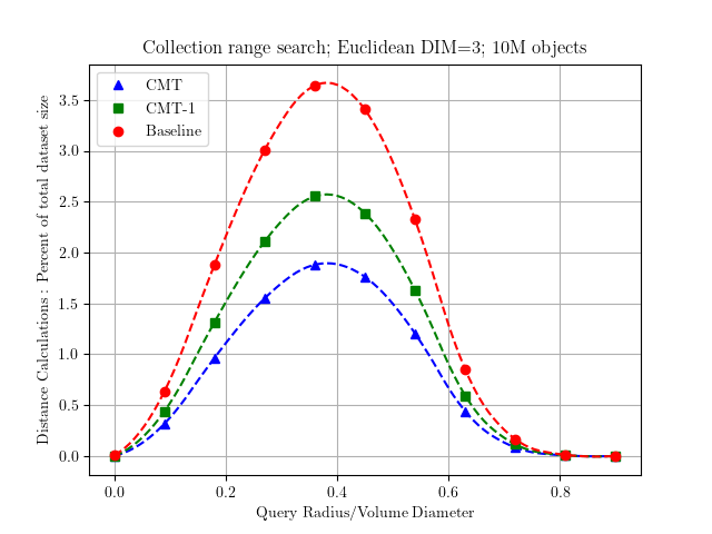
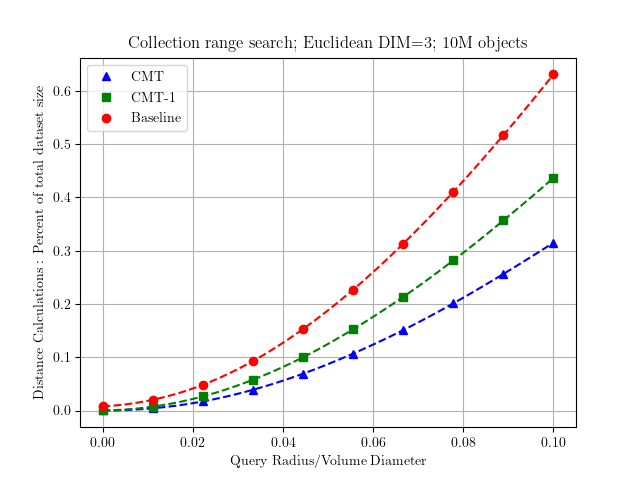
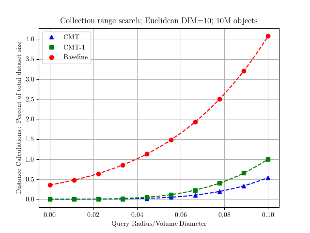
Our first battery of tests are performed on datasets of $10^{7}$ uniformly-distributed Euclidean-space objects in $3$ and $10$ dimensions. Figures 2(a) and 2(b) show the fraction of objects for which distance calculations are performed as a function of query radius/volume. As the query radius increases, the number of distance calculations can be expected to increase until the query volume becomes so large that collection begins to dominate (i.e., an increasing number of objects can be identified as satisfying the query without need for individual distance calculations) and this is clearly seen. CMT performs roughly half as many distance calculations as Baseline across most of the range of possible query radii, and the performance of CMT-1 is roughly betwen that of CMT and Baseline. The performance of CMT-1 indicates that only one generation of ancestral information is sufficient to provide more than half of the pruning power of CMT in this case.

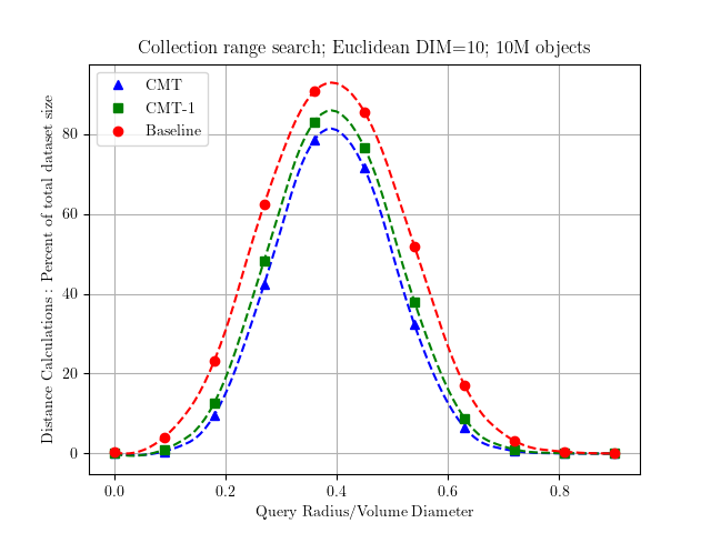
Figures 2(c) and 2(d) perform analogous tests but in $10$ dimensions. Because intrinsic difficulty of search increases with dimensionality, it is not surprising to see that the advantage of CMT over Baseline increases from a factor of $2$ to a factor of $5$ reduction in needed distance calculations. On the other hand, uniformly-distributed objects in Euclidean space make the problem relatively easy in the sense that it is amenable to effective approximate search methods based on grid or orthogonal range-search structures such as the kd-tree. This may partly explain why the performance of CMT-1 degrades less relative to that of CMT when the dimensionality is increased from $3$ to $10$.

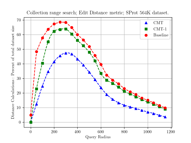
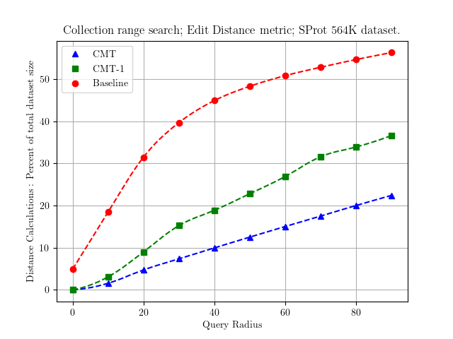
Figures 2(e) and 2(f) show results for edit-distance (more specifically Levenshtein distance [10, 11]) range queries on the 2021 SwissProt database of $564$K protein sequences [12], with an average protein length of 360 amino acids. Figure 2(e) shows that the performance of CMT-1 is degraded significantly relative to CMT and approaches that of Baseline. This tends to suggest that CMT-1’s lack of cascaded information beyond the parent significantly limits its pruning power, i.e., pruning information provided by distant ancestors for CMT tends to increase with problem difficulty.

Figures 2(a), 2(c), and 2(e) show the power of collection for large retrieval sets due to large query volumes. Specifically, the number of distance calculations eventually plateaus and then diminishes with increasing search radius. Although conventional metric search structures examined in the literature have not exploited collection capability, we have equipped the Baseline range search algorithm to exploit collection. Without it, the number of distance calculations increases exponentially with query radius and cannot be meaningfully graphed against searches performed with collection.

6 k-Nearest Neighbor (kNN) Queries

The $k$-nearest neighbor query (or $K(q,k)$) asks for the $k$ objects in a dataset $S$ that are nearest to a given query object $q$. Unlike range queries, for which the order of tree traversal has no effect on performance (i.e., number of required distance calculations and/or node visitations), the ordering of nodes visited for kNN queries has a substantial effect. This is because the bounding radius for the currently-identified nearest $k$ objects during the search imposes a pruning constraint on how close future objects must be to $q$ in order to displace the farthest element of the current set of $k$ nearest objects. Thus, the sooner a “good” set of $k$ objects can be found, the sooner non-candidates can be pruned.

A priority queue provides precisely the needed means for steering the sequence of nodes visited to those with higher likelihood of containing objects nearer to $q$. This is achieved by computing a “priority” for each visited node and placing the node (with its priority) into the queue. The next node to be visited is then obtained as the node with highest priority in the queue. The resulting performance of the overall algorithm thus depends, of course, on the formula used to determine the priorities.

Given the distance $d(p,q)$ between query object $q$ and node object $p$, and the bounding radius for for $p$ that contains all objects in its associated subtree, a triangle inequality calculation can produce a lower bound on the distance to the nearest object in the subtree. Alternatively, a lower bound can be obtained for the distance of the nearest possible object outside the bounding radius of the node.

In the case of non-cascaded metric search trees, a lower-bound distance between $q$ and the nearest-neighbor in the subtree of the current node can be directly calculated. It is zero if $q$ is within the node’s bounding volume; otherwise it is the distance from $q$ to the maximum bounding volume that is guaranteed to not include and objects within the bounding volume of the node. In either case, the computed value is the obvious choice for use as a search priority. What is critical to note is that this leads to what is essentially a proximity-based greedy search of the tree.

For CMT, by contrast, multiple lower-bound distances can be computed: one from the current node, and one from use of the triangle inequality with the available distances $d(q,a_{i})$, $d(a_{i},p)$, and $d(q,p)$ for each ancestor object $a_{i}$. Because each represents a lower bound, the largest of the lower bounds represents the most informative estimate of the smallest distance to an object in the subtree, and it is used as the priority for the node by the CMT kNN query algorithm (given in Appendix C). In other words, the priority function exploits information available in the CMT that is not available to structures of linear $O(N)$ size. This permits the kNN search algorithm to pursue a risk-averse ordering of nodes rather than a greedy proximity-focused ordering.

6.1 Range-Optimal kNN Search

In the computer science literature, many data structures for satisfying orthogonal (also known as coordinate-aligned or box) queries have been developed that are amenable to proving rigorous worst-case complexity bounds on the search time. For example, the optimal linear-size range-search data structure [13] can provably satisfy multidimensional range queries in $O(N^{(1-1/d)}+m)$ time, where $d$ is the dimensionality of the space and $m$ is the number of retrieved objects.

Unfortunately, few rigorous claims can be made about the performance of metric search structures without reference to properties of the specific metric that will be used. This presents a challenge to metric search as a research area because performance can typically only be expressed in the form of limited empirical comparisons to other methods. We now propose a step forward in this regard by defining the optimality of a given kNN algorithm for a particular metric search structure in terms of its performance relative to a range query (without collection) on that search structure with assumed knowledge of the minimum-size bounding ball containing the $k$-nearest neighbors.

Definition: A $k$-nearest neighbor search algorithm is range-optimal if its empirically assessed performance (e.g., in terms of distance calculations or number of nodes visited) approaches that of the best range query algorithm for the search structure of interest when given the smallest search radius enclosing the $k$-nearest objects.

The rationale for this definition is that the satisfaction of a range query is not sensitive to the order in which the satisfying objects are identified during the search process. More specifically, whether or not a particular object satisfies the query can be determined in isolation (independently) without regard to knowledge about other objects in the dataset. In other words, the sole information available for pruning is given by the radius of the range query.

By contrast, a kNN search initially has no pruning information and therefore must dynamically acquire it in the form of a variable bounding radius at each point during the search process based on the objects examined up to that point. This means that an optimally-defined range query should represent a lower bound on the best performance possible for satisfying a kNN query.

It should be noted that optimality as defined here is search-structure-specific in that kNN performance is bounded by the best possible range-search algorithm for that structure. As an example, an unstructured dataset of size $n$ offers range-optimality in the trivial sense that both kNN and range searches must perform exactly $n$ distance calculations during an exhaustive brute-force examination of all objects in the dataset.

The value of the range-optimal kNN criterion is realized when assessing the relative performance of different priority-search methods for satisfying kNN queries on sophisticated data structures. Specifically, if a kNN method is found that achieves the same performance as a minimum-radius range query for the $k$-nearest neighbors, no other method can possibly perform better.

During the kNN tests discussed in the next section, we assessed the range-optimality of CMT and Baseline. We found CMT to be 99% range-optimal, which means that improvements to the CMT kNN search algorithm can at most reduce the number of distance calculations and/or node visitations by a small fraction. Baseline was similarly found to be between 97% and 99% range-optimal. This implies that empirically-observed performance advantages of CMT for kNN queries cannot be attributed to possible use of a highly suboptimal kNN query algorithm for the Baseline search tree.

6.2 Range-Bounded kNN Queries

As discussed earlier, the query model can be extended to a general pruning function over any number of application-relevant parameters, e.g.,

$$f(r,k,nv,dc,t,...)~{}<~{}\mbox{\em threshold}$$ (1)

where in isolation a bound $r$ defines an ordinary range query; $k$ defines a bound on the number of returned nearest neighbors; $nv$ defines a bound on nodes visited; $dc$ defines a bound on distance calculations; $t$ defines a bound on total execution time; and so on. Various multi-criteria pruning methods have been examined, often termed approximate queries when the criteria does not guarantee that the $m$ returned objects are the nearest $m$ objects [14, 15].

Of particular practical interest is the satisfaction of range-bounded kNN queries of the form $K(b,k)$, where $b$ defines a bound on the maximum range/radius and $k$ defines the number of nearest neighbors to be returned from within that bounded range. Its practical significance derives from the fact that a standard kNN query can be thought of as a type of dynamic range query in which which the range is progressively reduced during evaluation of the query based on the bounding radius of the current set of $k$-nearest neighbors. This means that the effective bounding radius is infinite until a first set of $k$ objects has been accumulated, and the maximum radius of those initial $k$ objects is likely to be much larger than that of the final returned set of $k$-nearest objects.

In applications for which it is known that objects beyond some radius are either not of interest, or that the radius is virtually guaranteed to contain the nearest $k$ objects, then the bound $b$ can provide substantial pruning capability early in the query process. As will be demonstrated in the next section, this can lead to orders-of-magnitude improvements in performance.

(a)

(b)

(c)

(d)

Figure 3: kNN Search Performance for Euclidean and Edit Distance Metrics - Subfigures $(a)$-$(c)$ show the number of distance calculations as a function of the selected number $k$ of returned nearest neighbors, with $(a)$ and $(b)$ showing that Baseline performs a factor of between $4$ and $5$ more distance calculations than CMT in both 3 and 10 dimensions. For the for ordinary kNN search with Edit Distance Metric on the SwissProt dataset, CMT queries visit about 20 percent less of the dataset than Baseline (Subfigure ($c$)). For range-bound queries, we see in Subfigure ($d$) that the CMT is a dramatic improvement over Baseline (e.g. for a radius that is two percent of the query length, the improvement is about 30 fold ).

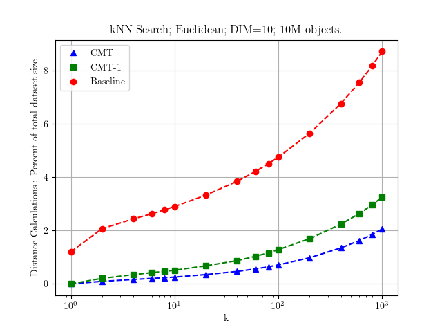
7 CMT k-Nearest Neighbor (kNN) Tests

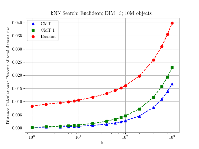
In this section we examine the satisfaction of kNN queries for CMT, CMT-1, and Baseline. Specifically, Figure 3 shows the the percentage of the dataset examined (i.e., requiring distance calculations) as a function of the number $k$ of returned nearest neighbors. To more realistically model practical usage, query objects were not chosen from the actual dataset. Thus, $k$=$1$ does not necessarily return an object of distance zero from the query object.

Figure 3(a) shows results for Euclidean kNN queries on a dataset of $10^{7}$ uniformly-distributed points in 3 dimensions for $k$ from 1 to 1000. At $k$=$100$ it can be seen that Baseline performs over 5 times as many distance calculations as CMT, and over 3 times as many as CMT-1. As $k$ approaches 1000, the performance of all three methods is degrading rapidly. The relative behavior of the three methods in 10 dimensions, shown in Figure 3(b) is qualitatively similar to that in 3 dimensions, but with almost two orders of magnitude more distance calculations per corresponding value of $k$.

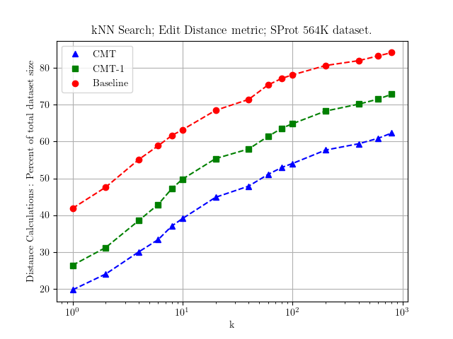
Figure 3(c) shows edit-distance kNN results for the same $564K$ protein sequence dataset as Figure 2. However, the discrete nature of edit distance does not admit a smooth functional relationship with $k$ because each increment of distance leads to an integral increase in the number of sequences such that there are typically many more than $k$ objects of strictly-equal distance to the query object, which accounts for the nonsmooth graphs in Figure 3(c).

Another issue that arises with kNN queries in practical applications is that the choice of $k$ may dramatically affect query complexity when one of the $k$ objects is much farther from the query object than the others. For example, the SwissProt dataset of protein sequences has high intrinsic dimensionality due to wide variation in sequence lengths such that $k$=$10$ can require $60\%$ of the dataset to be examined. In practice, however, the returning of sequences that are more than a factor of $2$ larger or smaller than the query sequence doesn’t make sense because the similarity is essentially equivalent to that between random sequences.

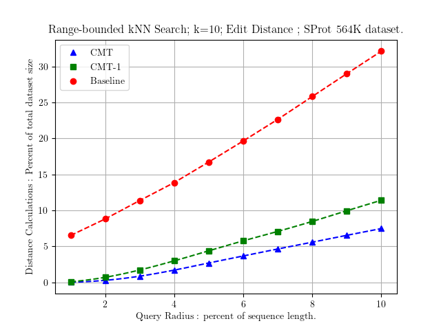
Figure 3(d) is more practically revealing by providing results for range-bounded kNN queries, $K(b,k)$, with $b$ determined as a percentage $p$ of the length of the query sequence. For $p$=$10$, the Baseline evaluations are reduced from about $60\%$ of the dataset size to about $35\%$, and for CMT the reduction is from about $40\%$ to $7\%$. For smaller ranges, the advantage of CMT over Baseline is even more dramatic. In the case of $p$=$<2$, for example, the number of distance calculations performed by CMT is $30$ times less than that of Baseline.

8 Discussion

In this paper we have introduced the notion of cascading as a means for permitting metric search algorithms to exploit more pruning information from distance calculations performed along each path of a search tree. The cascaded metric tree (CMT) is a concrete realization of this concept, and we have provided test results showing the performance advantages it provides for range (ball) queries and $k$-nearest neighbor (kNN) queries.

Our tests of the benefits provided strictly by cascading are novel in that we compare both against a Baseline metric search tree structure, which we believe serves as a fair proxy for prior-art methods, and a version of CMT, referred to as CMT-1, with only one level of cascading. The resulting test results give us confidence that independent comparisons of prior-art methods to the CMT will corroborate its significant advantages.

A contribution of this paper in the context of range queries is an emphasis on the importance of collection as being not only useful for reducing distance calculations needed for retrieval, but also for interactive query systems, e.g., that use counting queries to determine the number of objects that satisfy a given query without retrieving them. Although satisfaction of isolated counting queries on metric search structures is likely to be only marginally more efficient than retrieval queries, the number of counting queries performed in interactive data analysis applications may be proportionally much higher because of their iterative-refinement use in formulating range queries with practical-sized return sets.

Another contribution of potentially broader interest is our metric-independent definition of kNN algorithmic optimality, which we refer to as range-optimality, that can be assessed for any kNN algorithm as applied with any metric search structure for any choice of metric distance function. This is a step toward establishing more rigorous and objective statements about the performance of particular metric search structures and query algorithms.

A potentially more important practical contribution of the paper is our set of range and kNN edit-distance tests on the Swiss-Prot-X dataset, which contains 564k protein sequences. These tests remain far-removed from capturing the full scope and detail of the kinds of queries needed for practical sequence analysis, but they provide strong evidence of the potential to significantly outperform optimized brute-force methods as dataset sizes continue to increase.

Future work is needed to more fully assess the query requirements for large-scale use of metric search structures for applications relating to proteomic and genomic sequence analyses. These applications often require the finding of objects that are within a specified threshold on similarity – rather than distance – according to a highly complex non-metric similarity function.

Methods for converting similarity queries of this kind to metric distances have been examined in the bio-medical literature, but they tend to achieve only a relatively loose correspondence, i.e., the resulting metric search query is expected to return a superset of the desired objects. If this looseness proves unavoidable, the need for highly efficient metric search algorithms may be necessary to mitigate the resulting computational overhead.

Next-generation genomic and proteomic applications may also demand use of much more sophisticated metrics such as tree-edit [16] and graph-edit distance functions [17, 18]. Tree-edit distance, which determines the number of primitive edit operations necessary to transform one tree structure to another, can be expected to require $O(N^{3})$ rather than the $O(N^{2})$ complexity of string-edit distance [19, 20, 21, 22]. Graph-edit distance, by contrast, has been proven to be NP-Complete [23], and thus can be expected to demand computation time that is exponential in the size of the molecular structures contained in the search structure. Consequently, approximation methods may be necessary for both tree and graph-edit distance calculations [24], despite the possibility that queries (e.g., performed using CMT) may not equate to what would be obtained using the true distance functions.

In summary, we believe the results in this paper serve to advance the practical application of metric search algorithms to a wider array of real-world problem domains. Of particular interest are the enormous datasets presently being generated in biomedical, astronomical, and experimental physics applications. In such applications, reducing the number of distance calculations by only a factor of $4$ or $5$ can reduce the total processing time for a large data analysis program from a month down to a week.

APPENDICES

Sufficient detail is provided in the main text to understand and implement the CMT and its associated search algorithms. For completeness, however, we provide the following appendices with explicit pseudocode based on our C++ reference implementation.

Appendix A Basic CMT Range Query Algorithm

Pruning operations based on metric triangle-inequality tests can be neatly encapsulated for implementation using the concept of pruning distances. Consider the set $C$ of all objects in a node’s subtree, and let near and far be the distances from the node object to the nearest and farthest objects in $C$. The pruning distance is the distance the query object is outside of interval $D\coloneqq\left[\mbox{\em near,\, far}\right]$ (see Algorithm 1). When a node is visited during the search, if the search radius is less than the pruning distance, the node’s subtree can be excluded from the search. We extend the concept for use with ancestral distance intervals and define maximum pruning distance as the maximum of the pruning distances over the ancestral distance intervals.

PruningDistance(distancePQ, node, l) begin

      

      if $\textnormal{{distancePQ}}<\textnormal{{node}}.\textnormal{{near}}[l]$ then

             pruningDistance $\leftarrow\textnormal{{node}}.\textnormal{{near}}[l]-\textnormal{{distancePQ}}$

       end if

      else if $\textnormal{{distancePQ}}>\textnormal{{node}}.\textnormal{{far}}[l]$ then

             pruningDistance $\leftarrow\textnormal{{distancePQ}}-\textnormal{{node}}.\textnormal{{far}}[l]$

       end if

      else

             pruningDistance $\leftarrow 0$

       end if

      return pruningDistance

end

Algorithm 1 xCalculation of the pruning distance by the function $PruningDistance(d_{pq},n,0)$.

Algorithm 2 performs basic CMT range queries. Its recursive structure applied to the tree visits a node at most once. Upon visiting a node, the max pruning distance with respect to the set of ancestral objects is determined, if this is greater than the query radius then the current search path can be terminated. If the query object is not pruned at this step, then a distance calculation must be performed between the query object and the node object, which provides one more pruning test with respect to the bounding volume of the node. If the node object satisfies the query then it is added to the result set. Regardless, the distance between the query object and the node object is added to the list of ancestral objects for use in pruning tests at subsequently visited nodes along the current path in the tree, and the search proceeds recursively to the left subtree and then the right subtree.

BasicRangeQuery(query, node, stack) begin

      

      if  node is null then

             return

       end if

      

      maxPD $\leftarrow$ MaxPruningDistance (stack, node)

      if  $\textnormal{{maxPD}}\leq\textnormal{{query}}.searchRadius()$  then

            

            distance $\leftarrow\textnormal{{distance}}(\textnormal{{query}}.\textnormal{{object}},\textnormal{{node}}.\textnormal{{object}})$

            if $\textnormal{{distance}}\leq\textnormal{{query}}.searchRadius()$  then

                   query.addResult(node.object, distance)

             end if

            

            PD = PruningDistance (distance, node, 0)

            if  $\textnormal{{PD}}\leq\textnormal{{query}}.searchRadius()$  then

                  

                  stack.push( distance)

                  BasicRangeQuery (query, node.left, stack)

                  BasicRangeQuery (query, node.right, stack)

                  stack.pop()

             end if

            

       end if

      return

end

Algorithm 2 Basic CMT Range Query Algorithm

Appendix B Collection CMT Range Query Algorithm

Collection is an enhancement to the basic range query (Algorithm 2) with tests added to identify cases in which the query volume encloses a node’s bounding volume. We define the collection distance as the sum of the distance between the query object and the node object, plus the far component of the node’s distance interval. We also define a minimum collection distance as the minimum of the collection distances over the ancestral distance intervals. More intuitively, this represents the intersection of constraining bounding volumes of the ancestor objects and that of the current node. If the query volume contains this intersection volume then all objects in the subtree rooted at the current node must necessarily satisfy the query, and therefore they may be collected into the result set without need for explicit distance calculations.

Algorithm 3 performs CMT queries with collection. The algorithm is similar to algorithm 2 except for the addition of a test against the minimum collection distance and a test against the collection distance. When the distances are less than the search radius, all objects in the subtree (including the node object) are added to the result set.

CollectRangeQuery(query, node, stack) begin

      

      if  node is null then

             return

       end if

      

      maxPrunigDist $\leftarrow$ MaxPruningDistance (stack, node)

      if  $\textnormal{{maxPrunigDist}}\leq\textnormal{{query}}.searchRadius()$  then

            

            minCD $\leftarrow$ MinCollectionDistance (stack, node)

            if  $\textnormal{{minCD}}\leq\textnormal{{query}}.searchRadius()$  then

                   query.addSubtree(node, minCD)

             end if

            else

                  

                  distance $\leftarrow\textnormal{{distance}}(\textnormal{{query}}.\textnormal{{object}},\textnormal{{node}}.\textnormal{{object}})$

                  cd $\leftarrow\textnormal{{CollectionDistance}}(\textnormal{{distance}},\textnormal{{node}})$

                  if $\textnormal{{cd}}\leq\textnormal{{query}}.searchRadius()$  then

                         query.addSubtree(node, cd)

                   end if

                  else

                        

                        if $\textnormal{{distance}}\leq\textnormal{{query}}.searchRadius()$  then

                               query.addResult(node.object, distance)

                         end if

                        

                        pruningDist $\leftarrow$ PruningDistance (distance, node, 0)

                        if  $\textnormal{{pruningDist}}\leq\textnormal{{query}}.searchRadius()$  then

                              

                              stack.push( distance)

                              CollectRangeQuery (query, node.left, stack)

                              CollectRangeQuery (query, node.right, stack)

                              stack.pop()

                         end if

                        

                   end if

                  

             end if

            

       end if

      return

end

Algorithm 3 Full range query algorithm with collection/aggregation.

Appendix C CMT k-Nearest Neighbor (kNN) Algorithm

The CMT kNN query algorithm 4 uses a priority queue to determine the node visitation order. The priority queue provides the standard push() and pop() functions with members given in Table V.

TABLE V: Data Members of Priority-Queue Node

tree nodex	The tree node associated with the queue node.
parent	The parent queue node of the queue node.
distance	The distance between the tree node object and
	the query object.
priority	Measure of likelihood that close neighbors
	will be found in the subtree of the tree node.

The max pruning distance between the tree node and the query object is used for the priority, causing the search algorithm to preferentially visit nodes with greater likelihood of being pruned.

The algorithm visits a tree node by removing a queue node from the priority queue. The tree node is pruned if its priority (i.e., max pruning distance) is greater than the search radius. The distance between the query and node objects is then calculated; and if the object is within the current range then it is added to the result set, and if the size of the set exceeds $k$ then the farthest of the $k+1$ objects is removed and the minimum bounding radius of the remaining $k$ objects is updated. This bounding radius (distance) is also used to determine the max pruning distances of the two child nodes, and if they cannot be immediately pruned then they are each placed into the priority queue with their respective max pruning distances as their priorities. This means that a pruning test is applied both before the object is added to the queue and when it is later removed from the queue, where the latter test can be productive if the bounding radius of the $k$ objects has decreased in the interim.

kNNQuery(query, queue) begin

      

      while queue is not empty do

             queueNode $\leftarrow$ queue.pop

            node $\leftarrow\textnormal{{queueNode}}.\textnormal{{node}}$

            maxPruningDist $\leftarrow\textnormal{{queueNode}}.priority$

            if  $\textnormal{{maxPruningDist}}\leq\textnormal{{query}}.searchRadius()$  then

                  

                  distance $\leftarrow\textnormal{{distance}}(\textnormal{{query}}.\textnormal{{object}},\textnormal{{node}}.\textnormal{{object}})$

                  if $\textnormal{{distance}}\leq\textnormal{{query}}.searchRadius()$  then

                        

                        query.addResult(node.object, distance)

                   end if

                  

                  queueNode.dist $\leftarrow$ distance

                  if  $\textnormal{{PruningDistance}}(\textnormal{{distance}},\textnormal{{node}},0)\leq\textnormal{{query}}.searchRadius()$  then

                        

                        if  $\textnormal{{node}}.\textnormal{{left}}\neq\textnormal{{null}}$  then

                              

                              priority $\leftarrow$ MaxPruningDistance (queueNode, node.left)

                              if  $\textnormal{{priority}}\leq\textnormal{{query}}.searchRadius()$  then

                                    

                                    queue.push(new QueueNode (node.left, queueNode, priority))

                               end if

                              

                         end if

                        

                        if  $\textnormal{{node}}.\textnormal{{right}}\neq\textnormal{{null}}$  then

                              

                              priority $\leftarrow$ MaxPruningDistance (queueNode, node.right)

                              if  $\textnormal{{priority}}\leq\textnormal{{query}}.searchRadius()$  then

                                    

                                    queue.push(new QueueNode (node.right, queueNode, priority))

                               end if

                              

                         end if

                        

                   end if

                  

             end if

            

       end while

      

      return

end

Algorithm 4 CMT $k$NN Query algorithm

Appendix D Tree Construction

In the context of spatial search trees, the term “pivot” is commonly used to refer to an object used to discriminate between partitions of a dataset. Typically, the pivot object at a node is selected/determined during construction of the tree to define a partition of the dataset, and that object is stored at a node for subsequent use by a search algorithm to prune the traversal of certain subtrees. In the more general case, the pivot objects used for partitioning during the construction process need not be the same objects as those stored for use during the search process. In other words, a distinction must be made between partition pivots and search pivots, and we will explicitly distinguish between the two when there is potential ambiguity based on the context of the discussion.

It should be noted that the general the CMT definition does not specifically prescribe the manner of partitioning and selection of search pivots. Ideally, the search performance properties of the tree should be relatively invariant to discretion applied during the construction process, i.e., search efficiency should not depend on meticulous tailoring of the construction algorithm to exploit assumed characteristics of datasets arising in a particular application. However, the degree to which this ideal is achieved must be empirically assessed by examining different construction algorithms. For our tests we simply choose each partitioning pivot at random and then compute the median distance to the remaining objects to obtain a balanced partition. If the median distance is not unique, then each object with distance equal to the median will be arbitrarily assigned to one of the two subsets such that equal cardinality is maintained. This method ensures that the resulting tree is balanced with $O(\log N)$ height, which minimizes CMT memory requirements by limiting the maximum number of query pivots at any given node to $O(\log N)$. We refer to this as balanced object median (BOM) partitioning.

The CMT construction of Algorithm 6 is preceded by a pre-processing of a set $O$ of objects by allocating a set $S$ of nodes with $|S|=|O|=N$, with the assigning of one object to each node. The tree is then constructed by recursively applying a procedure that selects a node $p$ from $S$, which will also serve as a root or parent of the current subtree. This is followed by partitioning the set $\{S\setminus\{p\}\}$ into two subsets, $S_{l}$ and $S_{r}$, which will be recursively constructed as the left and right subtrees, respectively. In the process of partitioning, the metric distances between $p$ and each object in $\{S_{l}\cup S_{r}\}$ are calculated. Additionally, the minimum and maximum of those distances are stored in the near and far data members of the node’s distance interval. Finally, a vector $p.pDistance{[}{]}$ is stored as a member of each node and contains the distance between the node object and each of the node’s ancestor objects. The function ComputeADIV() uses these vectors to compute, for the local root, a distance interval per each ancestor.

ComputeADIV(pnode, cnodes, depth) begin

      

      for $l\in\left[0,\textnormal{{depth}}\right)$ do

            

            pdl $\leftarrow\textnormal{{depth}}-l-1$

            nearest $\leftarrow\underset{node\in{\textnormal{{cnodes}}\cup\textnormal{{pnode}}}}{min\{node.\textnormal{{pDistances}}[\textnormal{{pdl}}]\}}$

            furthest $\leftarrow\underset{node\in{\textnormal{{cnodes}}\cup\textnormal{{pnode}}}}{max\{node.\textnormal{{pDistances}}[\textnormal{{pdl}}]\}}$

            pnode.near[$l$] $\leftarrow\textnormal{{nearest}}$

            pnode.far[$l$] $\leftarrow\textnormal{{furthest}}$

       end for

      

end

BuildCMT(nodes, depth) begin

       if  $|\textnormal{{nodes}}|==0$ then

             return null

       end if

      

      if $|\textnormal{{nodes}}|==1$ then

             root $\leftarrow$ first { nodes }

            return root

       end if

      

      root $\leftarrow$ a random node $\in$ nodes

      nodes $\leftarrow\{\textnormal{{nodes}}\setminus\textnormal{{root}}\}$

      for node $\in$ nodes do

             node.distance [ depth ] $\leftarrow\textnormal{{distance}}(\textnormal{{node}}.object,\textnormal{{root}}.object)$

       end for

      

      root.near[0] $\leftarrow\underset{\textnormal{{node}}\in\textnormal{{nodes}}}{\mathrm{min}\{\textnormal{{node}}.\textnormal{{distance}}[\textnormal{{depth}}]\}}$

      root.far[0] $\leftarrow\underset{\textnormal{{node}}\in\textnormal{{nodes}}}{\mathrm{max}\{\textnormal{{node}}.\textnormal{{distance}}[\textnormal{{depth}}]\}}$

      MedDist $\leftarrow$ median distance to random pivot

      left $\leftarrow$ {$\textnormal{{node}}\in\textnormal{{nodes}}\mid\textnormal{{node}}.\textnormal{{distance}}[\textnormal{{depth}}]<$ MedDist }

      right $\leftarrow\{\textnormal{{nodes}}\setminus\textnormal{{left}}\}$

      root.right$\leftarrow$BuildCMT(right, $\textnormal{{depth}}+1$)

      root.left$\leftarrow$BuildCMT(left, $\textnormal{{depth}}+1$)

      ComputeADIV ( root, nodes, depth)

      return root

end

Algorithm 5 xCalculating the ancestral distance intervals for node $pnode$

Algorithm 6 xComputeADIV() - Building the CMT with random pivots and BOM partitioning.

ComputeADIV() (Algorithm 6) computes ancestral distance intervals for the current node. This algorithm is executed for a given node after its children are recursively processed by the calling algorithm. When this algorithm is called for node $pnode$ at depth $d$ and with descendant node set $cnodes$, each descendant node already has $d+1$ distance values in its own $pDistances$ array. (The index into $pDistances$ starts with the root node of the entire tree indexed as $nd.pDistance[0]$.) The construction algorithm for the Baseline tree is nearly identical to Algorithm 6, and the number of distance function evaluations is the same, but no ancestral information is maintained.

D.1 Tree construction complexity

The computational complexity of building CMT with BOM partitioning is technically $O(N\log^{2}N)$ because the tree has $O(N)$ nodes with $O(\log N)$ scalar ancestral distance values. However, the $O(N\log^{2}N)$ component of the runtime is simply due to the maintenance of $O(\log N)$ ancestral distances per node. Thus the coefficient of the $O(N\log^{2}N)$ component is relatively small compared to that of the $O(N\log N)$ distance calculations performed by ComputeADIV(). Consequently, for any nontrivial distance function the practical build time for the tree will be dominated by the $O(N\log N)$ component.

References

- [1] H. Samet, Foundations of multidimensional and metric data structures, ser. Morgan Kaufmann series in data management systems. Academic Press, 2006.
- [2] P. Zezula, G. Amato, V. Dohnal, and M. Batko, Similarity search: the metric space approach. Springer Science & Business Media, 2006, vol. 32.
- [3] E. Chávez, G. Navarro, R. Baeza-Yates, and J. L. Marroquín, “Searching in metric spaces,” ACM computing surveys (CSUR), vol. 33, no. 3, pp. 273–321, 2001.
- [4] J. K. Uhlmann, “Implementing metric trees to satisfy general proximity/similarity queries,” NRL Code 5570 Report (and available as Advanced Information Technology, Code 5580, Technical Report: AT-92-006), 1991, https://apps.dtic.mil/sti/pdfs/ADA283150.pdf.
- [5] J. Uhlmann, “Real-time decision support with metric trees,” in 8th Annual Conference on Command and Control Decision Aids. Joint Services Decision Aids Working Group (DAWG), June 1991.
- [6] P. N. Yianilos, “Locally lifting the curse of dimensionality for nearest neighbor search (extended abstract),” in Proceedings of the Eleventh Annual ACM-SIAM Symposium on Discrete Algorithms, ser. SODA ’00. USA: Society for Industrial and Applied Mathematics, 2000, p. 361–370.
- [7] T. H. Cormen, C. E. Leiserson, R. L. Rivest, and C. Stein, Introduction to Algorithms (Chapter 11: Hash Tables), 2nd ed. The MIT Press, 2001.
- [8] J. Uhlmann, “Satisfying general proximity/similarity queries with metric trees,” Information Processing Letters, vol. 40, pp. 201–213, 1991.
- [9] P. Yianilos, “Data structures and algorithms for nearest neighbor search in general metric spaces,” in SODA ’93, 1993.
- [10] M. Sosic and M. Sikic, “Edlib: a C/C++ library for fast, exact sequence alignment using edit distance,” Bioinformatics, vol. 33, no. 9, pp. 1394–1395, 01 2017. [Online]. Available: https://doi.org/10.1093/bioinformatics/btw753
- [11] G. Navarro, “A guided tour to approximate string matching,” ACM Comput. Surv., vol. 33, no. 1, pp. 31–88, mar 2001. [Online]. Available: https://doi.org/10.1145/375360.375365
- [12] A. Bairoch and R. Apweiler, “The swiss-prot protein sequence database and its supplement trembl in 2000,” Nucleic acids research, vol. 28(1), pp. 45–48, 2000. [Online]. Available: https://doi.org/10.1093/nar/28.1.45
- [13] J. L. Bentley, “Multidimensional binary search trees used for associative searching,” Communications of the ACM, vol. 18, no. 9, pp. 509–517, 1975.
- [14] R. Mao, W. Xu, W. S. Willard, S. R. Ramakrishnan, and D. P. Miranker, “Mobios index: Support distance-based queries in bioinformatics,” 2006.
- [15] W. Xu, D. Miranker, R. Mao, and S. Ramakrishnan, “Anytime k-nearest neighbor search for database applications,” in 2008 IEEE 24th International Conference on Data Engineering Workshop, 2008, pp. 426–435.
- [16] C. Laitang, K. Pinel-Sauvagnat, and M. Boughanem, “DTD Based Costs for Tree-Edit Distance in Structured Information Retrieval,” in Proceedings of the 35th European Conference on Information Retrieval Research: Advances in Information Retrieval, ser. Lecture Notes in Computer Science, vol. 7814. Springer International Publishing, 2013, pp. 158–170.
- [17] K. Riesen and H. Bunke, “Iam graph database repository for graph based pattern recognition and machine learning,” in Structural, Syntactic, and Statistical Pattern Recognition, N. da Vitoria Lobo, T. Kasparis, F. Roli, J. T. Kwok, M. Georgiopoulos, G. C. Anagnostopoulos, and M. Loog, Eds. Berlin, Heidelberg: Springer Berlin Heidelberg, 2008, pp. 287–297.
- [18] Z. Zeng, A. K. H. Tung, J. Wang, J. Feng, and L. Zhou, “Comparing Stars: On Approximating Graph Edit Distance,” Proceedings of the VLDB Endowment, vol. 2, no. 1, pp. 25–36, 2009.
- [19] A. Backurs and P. Indyk, “Edit distance cannot be computed in strongly subquadratic time (unless seth is false),” in Proceedings of the Forty-Seventh Annual ACM Symposium on Theory of Computing, ser. STOC ’15. New York, NY, USA: Association for Computing Machinery, 2015, pp. 51–58. [Online]. Available: https://doi.org/10.1145/2746539.2746612
- [20] A. Andoni, R. Krauthgamer, and K. Onak, “Polylogarithmic approximation for edit distance and the asymmetric query complexity,” 2010 IEEE 51st Annual Symposium on Foundations of Computer Science, pp. 377–386, 2010.
- [21] S. Schwarz, M. Pawlik, and N. Augsten, “A new perspective on the tree edit distance,” in Similarity Search and Applications, C. Beecks, F. Borutta, P. Kröger, and T. Seidl, Eds. Cham: Springer International Publishing, 2017, pp. 156–170.
- [22] M. Pawlik and N. Augsten, “Rted: A robust algorithm for the tree edit distance,” Proc. VLDB Endow., vol. 5, no. 4, pp. 334–345, Dec. 2011. [Online]. Available: http://dl.acm.org/citation.cfm?id=2095686.2095692
- [23] Z. Abu-Aisheh, R. Raveaux, J.-Y. Ramel, and P. Martineau, “An Exact Graph Edit Distance Algorithm for Solving Pattern Recognition Problems,” in 4th International Conference on Pattern Recognition Applications and Methods 2015, Lisbon, Portugal, Jan. 2015. [Online]. Available: https://hal.archives-ouvertes.fr/hal-01168816
- [24] K. Riesen, Structural Pattern Recognition with Graph Edit Distance - Approximation Algorithms and Applications, ser. Advances in Computer Vision and Pattern Recognition. Springer, 2015. [Online]. Available: https://doi.org/10.1007/978-3-319-27252-8