Learning Bayesian Networks in the Presence of Structural Side Information

Abstract

We study the problem of learning a Bayesian network (BN) of a set of variables when structural side information about the system is available. It is well known that learning the structure of a general BN is both computationally and statistically challenging. However, often in many applications, side information about the underlying structure can potentially reduce the learning complexity. In this paper, we develop a recursive constraint-based algorithm that efficiently incorporates such knowledge (i.e., side information) into the learning process. In particular, we study two types of structural side information about the underlying BN: (I) an upper bound on its clique number is known, or (II) it is diamond-free. We provide theoretical guarantees for the learning algorithms, including the worst-case number of tests required in each scenario. As a consequence of our work, we show that bounded treewidth BNs can be learned with polynomial complexity. Furthermore, we evaluate the performance and the scalability of our algorithms in both synthetic and real-world structures and show that they outperform the state-of-the-art structure learning algorithms.

1 Introduction

Bayesian networks (BNs) are probabilistic graphical models that represent conditional dependencies in a set of random variables via directed acyclic graphs (DAGs). Due to their succinct representations and power to improve the prediction and to remove systematic biases in inference (Pearl 2009; Spirtes et al. 2000), BNs have been widely applied in various areas including medicine (Flores et al. 2011), bioinformatics (Friedman et al. 2000), ecology (Pollino et al. 2007), etc. Learning a BN from data is in general NP-hard (Chickering, Heckerman, and Meek 2004). However, any type of side information about the network can potentially reduce the complexity of the learning task.

BN structure learning algorithms are of three flavors: constraint-based, e.g., parent-child (PC) algorithm (Spirtes et al. 2000), score-based, e.g., (Chickering 2002; Solus, Wang, and Uhler 2017; Zheng et al. 2018; Zhu, Ng, and Chen 2020), and hybrid, e.g., MMHC algorithm (Tsamardinos, Brown, and Aliferis 2006).

Although constraint-based methods do not require any assumptions about the underlying generative model, they often require conditional independence (CI) tests with large conditioning sets or a large number of CI tests which grows exponentially as the number of variables increases. Often in practice, we have side information about the network that can improve learning accuracy or reduce complexity. We show in this work that such side information can reduce the learning complexity to polynomial in terms of the number of CI tests. Our main contributions are as follows.

• We propose a constraint-based Recursive Structure Learning (RSL) algorithm to recover BNs. In addition, we study two types of structural side information: (I) an upper bound on the clique number of the graph is known, or (II) the graph is diamond-free. In each case, we provide a learning algorithm. RSL follows a divide-and-conquer approach: it breaks the learning problem into several sub-problems that are similar to the original problem but smaller in size by eliminating removable variables (see Definition 1). Thus, in each recursion, both the size of the conditioning sets and the number of CI tests decrease.

• Learning BNs with bounded treewidth has recently attracted attention. Works such as (Korhonen and Parviainen 2013; Nie et al. 2014; Ramaswamy and Szeider 2021) aim to develop learning algorithms for BNs when an upper bound on the treewidth of the graph is given as side information. Assuming bounded treewidth is more restrictive than bounded clique number assumption, i.e., having a bound on the treewidth implies an upper bound on the clique number of the network. Hence, our proposed algorithm with structural side information of type (I) can also learn bounded treewidth BNs. However, our algorithm has polynomial complexity, while the state-of-the-art exact learning algorithms have exponential complexity.

• We show that when the clique number of the underlying BN is upper bounded by $m$, i.e., $\omega(\mathcal{G})\!\leq\!m$ (See Table 1 for the graphical notations), our algorithm requires $\mathcal{O}(n^{2}+n\Delta_{in}^{m+1})$ CI tests (Theorem 1). Furthermore, when the graph is diamond-free, our algorithm requires $\mathcal{O}(n^{2}+n\Delta_{in}^{3})$ CI tests (Theorem 2). These bounds significantly improve over the state of the art.

	$n$	Number of variables
	$\Delta(\mathcal{G})$	Maximum degree of DAG $\mathcal{G}$
	$\Delta_{in}(\mathcal{G})$	Maximum in-degree of DAG $\mathcal{G}$
	$\omega(\mathcal{G})$	Clique number of graph $\mathcal{G}$
	$N_{\mathcal{G}}(X)$	Neighbors of $X$ in DAG $\mathcal{G}$
	$Ch_{\mathcal{G}}(X)$	Children of $X$ in DAG $\mathcal{G}$
	$Pa_{\mathcal{G}}(X)$	Parents of $X$ in DAG $\mathcal{G}$
	$CP_{\mathcal{G}}(X)$	Co-parents of $X$ in DAG $\mathcal{G}$
	$Mb_{\mathbf{V}}(X)$	Markov boundary of $X$ among set $\mathbf{V}$
	$\alpha(\mathcal{G})$	Maximum Mb size of $\mathcal{G}$

Table 1: Graphical notations that we use in this paper.

Related work:

Herein, we review the relevant work on BN learning methods as well as those with side information.

The PC algorithm (Spirtes et al. 2000) is a classical example of constraint-based methods that requires $\mathcal{O}(n^{\Delta})$ number of CI tests. CS (Pellet and Elisseeff 2008) and MARVEL (Mokhtarian et al. 2021) are two examples that focus on BN structure learning with small number of CI tests by using the Markov boundaries (Mbs). This results in $\mathcal{O}(n^{2}2^{\alpha})$ and $\mathcal{O}(n^{2}+n\Delta_{\text{in}}^{2}2^{\Delta_{\text{in}}})$ number of CI tests for CS and MARVEL, respectively. On the other hand, methods such as GS (Margaritis and Thrun 1999), MMPC (Tsamardinos, Aliferis, and Statnikov 2003a), and HPC (de Morais and Aussem 2010) focus on reducing the size of the conditioning sets in their CI tests. However, the aforementioned methods are not equipped to take advantage of side information. Table 2 compares the complexity of various constraint-based algorithms in terms of their CI tests. RSL_ω and RSL_D are our proposed algorithms when an upper bound on the clique number is given and when the BN is diamond-free, respectively. Note that in general, $\Delta_{\text{in}}\leq\Delta\leq\alpha$, and in a DAG with a constant in-degree, $\Delta$ and $\alpha$ can grow linearly with the number of variables.

	Algorithm	#CI tests
	PC	$\mathcal{O}(n^{\Delta})$
	GS	$\mathcal{O}(n^{2}+n\alpha^{2}2^{\alpha})$
	MMPC, CS	$\mathcal{O}(n^{2}2^{\alpha}$)
	MARVEL	$\mathcal{O}(n^{2}+n\Delta_{in}^{2}2^{\Delta_{in}})$
	RSLD	$\mathcal{O}(n^{2}+n\Delta_{in}^{3})$
	RSLω	$\mathcal{O}(n^{2}+n\Delta_{in}^{m+1})$

Table 2: Required number of CI tests in the worst case by various algorithms.

Side information about the underlying generative model has been harnessed for structure learning in limited fashion, e.g., (Sesen et al. 2013; Flores et al. 2011; Oyen, Anderson, and Anderson-Cook 2016; McLachlan et al. 2020). As an example, (Takeishi and Kawahara 2020) propose an approach to incorporate side knowledge about feature relations into the learning process. (Shimizu 2019) and (Sondhi and Shojaie 2019) study the structure learning problem when the data is from a linear structural equation model and propose LiNGAM and reduced PC algorithms, respectively. (Claassen, M. Mooij, and Heskes 2013; Zheng et al. 2020) consider learning sparse BNs. In particular, (Claassen, M. Mooij, and Heskes 2013) show that in sparse setting, BN recovery is no longer NP-hard, even in the presence of unobserved variables. That is for sparse graphs with maximum node degree of $\Delta$, a sound and complete BN can be obtained by performing $\mathcal{O}(n^{2(\Delta+2)})$ CI tests.

Side information has been incorporated into score-based methods in limited fashions too, e.g., (Chen et al. 2016; Li and van Beek 2018; Bartlett and Cussens 2017). The side information in the aforementioned works is in the form of ancestral constraints which are about the absence or presence of a directed path between two vertices in the underlying BN. (Bartlett and Cussens 2017) cast this problem as an integer linear program. The proposed method by (Chen et al. 2016) recovers the network with guaranteed optimality but it does not scale beyond 20 random variables. The method by (Li and van Beek 2018) scales up to 50 variables but it does not provide any optimality guarantee.

Another related problem is optimizing $\sum_{v\in\mathbf{V}}f_{v}(Pa(v))$ over a set of DAGs with vertices $\mathbf{V}$ and parent sets $\{Pa(v)\}_{v\in\mathbf{V}}$. In this problem $\{f_{v}(\cdot)\}_{v\in\mathbf{V}}$ is a set of predefined local score functions. This problem is NP-hard (Chickering, Heckerman, and Meek 2004). Note that the BN structure learning can be formulated as a special case of this problem by selecting appropriate local score functions. (Korhonen and Parviainen 2013) introduce an exact algorithm for solving this problem with complexity $3^{n}n^{t+\mathcal{O}(1)}$ under a constraint that the optimal BN has treewidth at most $t$. (Elidan and Gould 2008) propose a heuristic algorithm that finds a sub-optimal DAG with bounded treewidth which runs in time polynomial in $n$ and $t$. Knowing a bound on the treewidth is yet another type of structural side information that is more restrictive than our structural assumptions. Therefore, our algorithm in Section 4 can learn bounded treewidth BNs with polynomial complexity, i.e., $\mathcal{O}(n^{2}+n\Delta_{in}^{t+2})$, where $t$ is a bound on the treewidth and $\Delta_{in}<n$.

(Korhonen and Parviainen 2015) is another score-based method that study the BN structure learning when an upper bound $k$ on the vertex cover number of the underlying BN is available. Their algorithm has complexity $4^{k}n^{2k+\mathcal{O}(1)}$. Since the vertex cover number of a graph is greater than its clique number minus one, then our algorithm in Section 4 can also recover a bounded vertex cover numbers BN with complexity $\mathcal{O}(n^{2}+n\Delta_{in}^{k+2})$. (Grüttemeier and Komusiewicz 2020) consider the structural constraint that the moralized graph can be transformed into a graph with maximum degree one by at most $r$ vertex deletions. They show that under this constraint, an optimal network can be learned in $n^{\mathcal{O}(r^{2})}$ time.

2 Preliminaries

Throughout the paper, we use capital letters for random variables and bold letters for sets. Also, the graphical notations are presented in Table 1.

A graph is defined as a pair $\mathcal{G}=(\mathbf{V},\mathbf{E})$ where $\mathbf{V}$ is a finite set of vertices and $\mathbf{E}$ is the set of edges. If $\mathbf{E}$ is a set of unordered pairs of vertices, the graph is called undirected and if it is a set of ordered pairs, it is called directed. An undirected graph is called complete if $\mathbf{E}$ contains all edges. A directed acyclic graph (DAG) is a directed graph with no directed cycle. In an edge $(X,Y)\in\mathbf{E}$ (or $\{X,Y\}\in\mathbf{E}$, in case of an undirected graph), the vertices $X$ and $Y$ are the endpoints of that edge and they are called neighbors. Let $\mathcal{G}=(\mathbf{V},\mathbf{E})$ be a (directed or undirected) graph and $\overline{\mathbf{V}}\subseteq\mathbf{V}$, then the induced subgraph $\mathcal{G}[\overline{\mathbf{V}}]$ is the graph whose vertex set is $\overline{\mathbf{V}}$ and whose edge set consists of all of the edges in $\mathbf{E}$ that have both endpoints in $\overline{\mathbf{V}}$. The skeleton of a graph ${\mathcal{G}}=(\mathbf{V},\mathbf{E})$ is its undirected version. The clique number of an undirected graph $\mathcal{G}$ is the number of vertices in the largest induced subgraph of $\mathcal{G}$ that is complete.

Let $\textbf{X},\textbf{Y}$, and $\mathbf{S}$ be three disjoint subsets of $\mathbf{V}$. We use $\textbf{X}\perp_{\mathcal{G}}\textbf{Y}|\mathbf{S}$ to indicate $\mathbf{S}$ d-separates X and Y in $\mathcal{G}$. In this case, the set $\mathbf{S}$ is called a separating set for X and Y. Suppose $P_{\mathbf{V}}$ is the joint probability distribution of $\mathbf{V}$. We use $\textbf{X}\perp\mkern-9.5mu\perp_{P_{\mathbf{V}}}\textbf{Y}|\mathbf{S}$ to denote the Conditional Independence (CI) of X and Y given $\mathbf{S}$. Also, a CI test refers to detecting whether $X\perp\mkern-9.5mu\perp_{P_{\mathbf{V}}}Y|\mathbf{S}$. A DAG $\mathcal{G}$ is said to be an independency map (I-map) of $P_{\mathbf{V}}$ if for every three disjoint subsets of vertices $\textbf{X},\textbf{Y}$, and $\mathbf{S}$ we have $X\perp_{\mathcal{G}}Y|\mathbf{S}\Rightarrow X\perp\mkern-9.5mu\perp_{P_{\mathbf{V}}}Y|\mathbf{S}$. A DAG $\mathcal{G}$ is a minimal I-map of $P_{\mathbf{V}}$ if it is an I-map of $P_{\mathbf{V}}$ and the resulting DAG after removing any edge is no longer an I-map of $P_{\mathbf{V}}$. A DAG $\mathcal{G}=(\mathbf{V},\mathbf{E})$ is called a Bayesian network (BN) of $P_{\mathbf{V}}$, if and only if $\mathcal{G}$ is a minimal I-map of $P_{\mathbf{V}}$. The joint probability distribution $P_{\mathbf{V}}$ with a BN $\mathcal{G}=(\mathbf{V},\mathbf{E})$ satisfies the Markov factorization property, that is $P_{\mathbf{V}}=\prod_{X\in\mathbf{V}}P_{\mathbf{V}}(X|\textit{Pa}_{\mathcal{G}}(X))$ (Pearl 1988).

A joint distribution $P_{\mathbf{V}}$ may have several BNs. The Markov equivalence class (MEC) of $P_{\mathbf{V}}$, denoted by $\langle P_{\mathbf{V}}\rangle$, is the set of all its BNs. It has been shown that two DAGs belong to a MEC if and only if they share the same skeleton and the same set of v-structures (Pearl 2009). A MEC $\langle P_{\mathbf{V}}\rangle$ can be uniquely represented by a partially directed graph called essential graph. A DAG $\mathcal{G}=(\mathbf{V},\mathbf{E})$ is called a dependency map (D-map) of $P_{\mathbf{V}}$ if for every three disjoint subsets of vertices $\textbf{X},\textbf{Y}$, and $\mathbf{S}$, $\textbf{X}\perp\mkern-9.5mu\perp_{P_{\mathbf{V}}}\textbf{Y}|\mathbf{S}$ implies $\textbf{X}\perp_{\mathcal{G}}\textbf{Y}|\mathbf{S}$. This property is also known as faithfulness in the causality literature (Pearl 2009). Furthermore, $\mathcal{G}$ is called a perfect map if it is both an I-map and a D-map of $P_{\mathbf{V}}$, i.e., $\textbf{X}\perp_{\mathcal{G}}\textbf{Y}|\mathbf{S}\iff\textbf{X}\perp\mkern-9.5mu\perp_{P_{\mathbf{V}}}\textbf{Y}|\mathbf{S}$. Note that if $\mathcal{G}$ is perfect map of $P_{\mathbf{V}}$, then it belongs to $\langle P_{\mathbf{V}}\rangle$, i.e., a perfect map is a BN.

Problem description:

The BN structure learning problem involves identifying $\langle P_{\mathbf{V}}\rangle$ from $P_{\mathbf{V}}$ on the population-level or from a set of samples of $P_{\mathbf{V}}$. As mentioned earlier, the constraint-based methods perform this task using a series of CI tests. In this paper, we consider the BN structure learning problem using a constraint-based method, when we are given structural side information about the underlying DAG.

3 Learning Bayesian networks recursively

Suppose $\mathcal{G}=(\mathbf{V},\mathbf{E})$ is a perfect map of $P_{\mathbf{V}}$ and let $\mathcal{H}$ denote its skeleton. Recall that learning $\langle P_{\mathbf{V}}\rangle$ requires recovering $\mathcal{H}$ and the set of v-structures of $\mathcal{G}$. It has been shown that finding a separating set for each pair of non-neighbor vertices in $\mathcal{G}$ suffices to recover its set of v-structures (Spirtes et al. 2000). Thus, we propose an algorithm called Recursive Structure Learning (RSL) that recursively finds $\mathcal{H}$ along with a set of separating sets $\mathbfcal{S}_{\mathbf{V}}$ for non-neighbor vertices in $\mathbf{V}$. The pseudocode of RSL is presented in Algorithm 1.

1:  Input: $\mathbf{V},\,P_{\mathbf{V}},\text{ SideInfo}$

2:  $\textit{Mb}_{\mathbf{V}}\leftarrow\textbf{ComputeMb}(\mathbf{V},\,P_{\mathbf{V}})$

3:  $(\mathcal{H},\,\mathbfcal{S}_{\mathbf{V}})\leftarrow\textbf{RSL}(\mathbf{V},\,P_{\mathbf{V}},\,\textit{Mb}_{\mathbf{V}},\text{ SideInfo})$

1:  RSL$(\overline{\mathbf{V}},\,P_{\overline{\mathbf{V}}},\,\textit{Mb}_{\overline{\mathbf{V}}},\text{ SideInfo})$

2:  if $|\overline{\mathbf{V}}|=1$ then

3:     return  $((\overline{\mathbf{V}},\varnothing),\varnothing)$

4:  else

5:     $X\leftarrow\textbf{FindRemovable}(\overline{\mathbf{V}},\,P_{\overline{\mathbf{V}}},\,\textit{Mb}_{\overline{\mathbf{V}}},\text{ SideInfo})$

6:     $(\textit{N}_{\mathcal{G}[\overline{\mathbf{V}}]}(X),\,\mathbfcal{S}_{X})\leftarrow\textbf{FindNeighbors}(X,\,\overline{\mathbf{V}},\,P_{\overline{\mathbf{V}}},\,\textit{Mb}_{\overline{\mathbf{V}}}(X),\text{ SideInfo})$

7:     $\textit{Mb}_{\overline{\mathbf{V}}\setminus\{X\}}\leftarrow\textbf{UpdateMb}(X,\,P_{\overline{\mathbf{V}}},\,\textit{N}_{\mathcal{G}[\overline{\mathbf{V}}]}(X),\,\textit{Mb}_{\overline{\mathbf{V}}})$

8:     $(\mathcal{H}[\overline{\mathbf{V}}\setminus\{X\}],\,\mathbfcal{S}_{\overline{\mathbf{V}}\setminus\{X\}})\leftarrow\textbf{RSL}(\overline{\mathbf{V}}\setminus\{X\},\,P_{\overline{\mathbf{V}}\setminus\{X\}},\,\textit{Mb}_{\overline{\mathbf{V}}\setminus\{X\}},\text{ SideInfo})$

9:     Construct $\mathcal{H}[\overline{\mathbf{V}}]$ by $\mathcal{H}[\overline{\mathbf{V}}\setminus\{X\}]$ and undirected edges between $X$ and $\textit{N}_{\mathcal{G}[\overline{\mathbf{V}}]}(X)$.

10:     $\mathbfcal{S}_{\overline{\mathbf{V}}}\leftarrow\mathbfcal{S}_{\overline{\mathbf{V}}\setminus\{X\}}\cup\mathbfcal{S}_{X}$

11:     return  $(\mathcal{H}[\overline{\mathbf{V}}],\,\mathbfcal{S}_{\overline{\mathbf{V}}})$

Algorithm 1 Recursive Structure Learning (RSL).

RSL’s inputs comprise a subset $\overline{\mathbf{V}}\subseteq\mathbf{V}$ with its joint distribution $P_{\overline{\mathbf{V}}}$ such that $\mathcal{G}[\overline{\mathbf{V}}]$ is a perfect map of $P_{\overline{\mathbf{V}}}$, and their Markov boundaries $\textit{Mb}_{\overline{\mathbf{V}}}$ (see Definition 2), along with structural side information, which can be either diamond-freeness, or an upper bound on the clique number. In this case, RSL outputs $\mathcal{H}[\overline{\mathbf{V}}]$ and a set of separating sets $\mathbfcal{S}_{\overline{\mathbf{V}}}$ for non-neighbor vertices in $\overline{\mathbf{V}}$. The RSL consists of three main sub-algorithms: FindRemovable, FindNeighbors, and UpdateMb. It begins by calling FindRemovable in line 5 to find a vertex $X\in\overline{\mathbf{V}}$ such that the resulting graph after removing $X$ from the vertex set, $\mathcal{G}[\overline{\mathbf{V}}\setminus\{X\}]$, remains a perfect map of $P_{\overline{\mathbf{V}}\setminus\{X\}}$. Afterwards, in line 6, FindNeighbors identifies the neighbors of $X$ in $\mathcal{G}[\overline{\mathbf{V}}]$ and a set of separating sets for $X$ and each of its non-neighbors in this graph. In lines 7 and 8, RSL updates the Markov boundaries and calls itself to learn the remaining graph after removing vertex $X$, i.e., $\mathcal{G}[\overline{\mathbf{V}}\setminus\{X\}]$, respectively. The two functions FindRemovable and FindNeighbors take advantage of the provided side information, as we shall discuss later.

As mentioned above, it is necessary for $\mathcal{G}[\overline{\mathbf{V}}]$ to remain a perfect map of $P_{\overline{\mathbf{V}}}$ at each iteration. This cannot be guaranteed if $X$ is chosen arbitrarily. (Mokhtarian et al. 2021) introduced the notion of removability in the context of causal graphs and showed that removable variables are the ones that preserve the perfect map assumption after the distribution is marginalized over them. In this work, we introduce a similar concept in the context of BN structure recovery.

Definition 1 (Removable).

Suppose $\mathcal{G}=(\mathbf{V},\mathbf{E})$ is a DAG and $X\in\mathbf{V}$. Vertex $X$ is called removable in $\mathcal{G}$ if the d-separation relations in $\mathcal{G}$ and $\mathcal{G}[\mathbf{V}\setminus\{X\}]$ are equivalent over $\mathbf{V}\setminus\{X\}$. That is, for any vertices $Y,Z\in\mathbf{V}\setminus\{X\}$ and $\mathbf{S}\subseteq\mathbf{V}\setminus\{X,Y,Z\}$,

$$Y\perp_{\mathcal{G}}Z|\mathbf{S}\iff Y\perp_{\mathcal{G}[\mathbf{V}\setminus\{X\}]}Z|\mathbf{S}.$$ (1)

Proposition 1.

Suppose $\mathcal{G}=(\mathbf{V},\mathbf{E})$ is a perfect map of $P_{\mathbf{V}}$. For each variable $X\in\mathbf{V}$, $\mathcal{G}[\mathbf{V}\setminus\{X\}]$ is a perfect map of $P_{\mathbf{V}\setminus\{X\}}$ if and only if $X$ is a removable vertex in $\mathcal{G}$.

All proofs appear in Appendix B.

Markov boundary (Mb):

Our proposed algorithm uses the notion of Markov boundary.

Definition 2 (Mb).

Suppose $P_{\mathbf{V}}$ is the joint distribution on $\mathbf{V}$. The Mb of $X\in\mathbf{V}$, denoted by $\textit{Mb}_{\mathbf{V}}(X)$, is a minimal set $\mathbf{S}\subseteq\mathbf{V}\setminus\{X\}$ s.t. $X\perp\mkern-9.5mu\perp_{P_{\mathbf{V}}}\mathbf{V}\setminus(\mathbf{S}\cup\{X\})|\mathbf{S}$. We denote $(\textit{Mb}_{\mathbf{V}}(X)\!:\>X\in\mathbf{V})$ by $\textit{Mb}_{\mathbf{V}}$.

Definition 3 (co-parent).

Two non-neighbor variables are called co-parents in $\mathcal{G}$, if they share at least one child. For $X\in\mathbf{V}$, the set of co-parents of $X$ is denoted by $\textit{CP}_{\mathcal{G}}(X)$.

If $\mathcal{G}$ is a perfect map of $P_{\mathbf{V}}$, for every vertex $X\in\mathbf{V}$, $\textit{Mb}_{\mathbf{V}}(X)$ is unique (Pearl 1988) and it is equal to

$$\textit{Mb}_{\mathbf{V}}(X)=\textit{Pa}_{\mathcal{G}}(X)\cup\textit{Ch}_{\mathcal{G}}(X)\cup\textit{CP}_{\mathcal{G}}(X).$$ (2)

The subroutines FindRemovable and FindNeighbors need the knowledge of Mbs to perform their tasks. Several constraint-based and scored-based algorithms have been developed in literature such as TC (Pellet and Elisseeff 2008), GS (Margaritis and Thrun 1999), and others (Tsamardinos et al. 2003) that can recover the Mbs of a set of random variables. Initially, any of the aforementioned algorithms could be used in ComputeMb to find $\textit{Mb}_{\mathbf{V}}$ and pass it to the RSL. After eliminating a removable vertex $X$, the Mbs of the remaining graph will change. Therefore, we need to update and pass $\textit{Mb}_{\overline{\mathbf{V}}\setminus\{X\}}$ to the next recall of RSL. This is done by function UpdateMb in line 7 of Algorithm 1. We propose Algorithm 2 for UpdateMb and prove its soundness and complexity in Proposition 2. Further discussion about this algorithm is presented in Appendix D.

1:  UpdateMb$(X,\,P_{\overline{\mathbf{V}}},\,\textit{N}_{\mathcal{G}[\overline{\mathbf{V}}]}(X),\,\textit{Mb}_{\overline{\mathbf{V}}})$

2:  $\textit{Mb}_{\overline{\mathbf{V}}\setminus\{X\}}\leftarrow(\textit{Mb}_{\overline{\mathbf{V}}}(Y)\!:\>Y\in\overline{\mathbf{V}}\setminus\{X\})$

3:  for $Y\in\textit{Mb}_{\overline{\mathbf{V}}}(X)$ do

4:     Remove $X$ from $\textit{Mb}_{\overline{\mathbf{V}}\setminus\{X\}}(Y)$.

5:  if $\textit{N}_{\mathcal{G}[\overline{\mathbf{V}}]}(X)=\textit{Mb}_{\overline{\mathbf{V}}}(X)$ then

6:     for $Y,Z\in\textit{N}_{\mathcal{G}[\overline{\mathbf{V}}]}(X)$ do

7:        if $Y\perp\mkern-9.5mu\perp_{P_{\overline{\mathbf{V}}}}Z|\textit{Mb}_{\overline{\mathbf{V}}\setminus\{X\}}(Y)\setminus\{Y,Z\}$ then

8:           Remove $Z$ from $\textit{Mb}_{\overline{\mathbf{V}}\setminus\{X\}}(Y)$

9:           Remove $Y$ from $\textit{Mb}_{\overline{\mathbf{V}}\setminus\{X\}}(Z)$

10:  return  $\textit{Mb}_{\overline{\mathbf{V}}\setminus\{X\}}$

Algorithm 2 Updates Markov boundaries (Mbs).

Proposition 2.

Suppose $\mathcal{G}[\overline{\mathbf{V}}]$ is a perfect map of $P_{\overline{\mathbf{V}}}$ and $X$ is a removable variable in $\mathcal{G}[\overline{\mathbf{V}}]$. Algorithm 2 correctly finds $\textit{Mb}_{\overline{\mathbf{V}}\setminus\{X\}}$ by performing at most $\binom{|\textit{N}_{\mathcal{G}[\overline{\mathbf{V}}]}(X)|}{2}$ CI tests.

4 Learning BN with known upper bound on the clique number

In this section, we consider the BN structure learning problem when we are given an upper bound $m$ on the clique number of the underlying BN and propose algorithms 3 and 4 to efficiently find removable vertices along with their neighbors. We denote the resulting RSL with these implementations of FindRemovable and FindNeighbors by RSL_ω. First, we present a sufficient removability condition in such networks, which is the foundation of Algorithm 3.

Lemma 1.

Suppose $\mathcal{G}=(\overline{\mathbf{V}},\mathbf{E})$ is a DAG and a perfect map of $P_{\overline{\mathbf{V}}}$ such that $\omega(\mathcal{G})\leq m$. Vertex $X\in\overline{\mathbf{V}}$ is removable in $\mathcal{G}$ if for any $\mathbf{S}\subseteq\textit{Mb}_{\overline{\mathbf{V}}}(X)$ with $\left|\mathbf{S}\right|\leq m-2$, we have

$$\forall Y,Z\in\textit{Mb}_{\overline{\mathbf{V}}}(X)\setminus\mathbf{S}\!:$$ (3)

$$\hskip 22.76228ptY\centernot{\perp\mkern-9.5mu\perp}_{P_{\overline{\mathbf{V}}}}Z|\big{(}\textit{Mb}_{\overline{\mathbf{V}}}(X)\cup\{X\}\big{)}\setminus\big{(}\{Y,Z\}\cup\mathbf{S}\big{)},$$

$$\text{and}\ \forall Y\in\textit{Mb}_{\overline{\mathbf{V}}}(X)\setminus\mathbf{S}\!:$$

$$\hskip 22.76228ptX\centernot{\perp\mkern-9.5mu\perp}_{P_{\overline{\mathbf{V}}}}Y|\textit{Mb}_{\overline{\mathbf{V}}}(X)\setminus(\{Y\}\cup\mathbf{S}).$$

Also, the set of vertices that satisfy Equation (3) is nonempty.

1:  FindRemovable($\overline{\mathbf{V}},\,P_{\overline{\mathbf{V}}},\,\textit{Mb}_{\overline{\mathbf{V}}},\,\text{ SideInfo (m)}$)

2:  $\textbf{X}=(X_{1},...,X_{|\overline{\mathbf{V}}|})\leftarrow\overline{\mathbf{V}}$

3:  Sort X s.t. $|\textit{Mb}_{\overline{\mathbf{V}}}(X_{1})|\leq|\textit{Mb}_{\overline{\mathbf{V}}}(X_{2})|\dots\leq|\textit{Mb}_{\overline{\mathbf{V}}}(X_{|\overline{\mathbf{V}}|})|.$

4:  for $i=1$ to $|\overline{\mathbf{V}}|$ do

5:     if (3) holds for $X=X_{i}$ then

6:        return  $X_{i}$

Algorithm 3 Finds a removable vertex.

Algorithm 3 first sorts the vertices in $\overline{\mathbf{V}}$ based on their Mb size and checks their removability, starting with the vertex with the smallest Mb. This ensures that both the number of CI tests and the size of the conditioning sets remain bounded.

Proposition 3.

Suppose $\mathcal{G}[\overline{\mathbf{V}}]$ is a DAG and a perfect map of $P_{\overline{\mathbf{V}}}$ s.t. $\omega(\mathcal{G[\overline{\mathbf{V}}]})\leq m$. Algorithm 3 returns a removable vertex in $\mathcal{G}[\overline{\mathbf{V}}]$ by performing $\mathcal{O}(|\overline{\mathbf{V}}|\Delta_{\textit{in}}(\mathcal{G}[\overline{\mathbf{V}}])^{m})$ CI tests.

We now turn to the function FindNeighbors. Recall that the purpose of this function is to find the neighbors of a removable vertex $X$ and its separating sets. Since for every vertex $Y\not\in\textit{Mb}_{\overline{\mathbf{V}}}(X)$, we have $Y\perp\mkern-9.5mu\perp_{P_{\overline{\mathbf{V}}}}X|\textit{Mb}_{\overline{\mathbf{V}}}(X)$, $\textit{Mb}_{\overline{\mathbf{V}}}(X)$ is a separating set for all vertices outside of $\textit{Mb}_{\overline{\mathbf{V}}}(X)$. Therefore, it suffices to find the non-neighbors of $X$ within $\textit{Mb}_{\overline{\mathbf{V}}}(X)$ or equivalently the co-parents of $X$. Next result characterizes the co-parents of a removable vertex $X$.

Lemma 2.

Suppose $\mathcal{G}[\overline{\mathbf{V}}]$ is a DAG and a perfect map of $P_{\overline{\mathbf{V}}}$ with $\omega(\mathcal{G[\overline{\mathbf{V}}]})\leq m$. Let $X\in\overline{\mathbf{V}}$ be a vertex that satisfies Equation (3) and $Y\in\textit{Mb}_{\overline{\mathbf{V}}}(X)$. Then, $Y\in\textit{CP}_{\mathcal{G}}(X)$ iff

$$\exists\mathbf{S}\subseteq\textit{Mb}_{\overline{\mathbf{V}}}(X)\setminus\{Y\}\!:\\ \left|\mathbf{S}\right|=(m-1)\,,\ \ X\perp\mkern-9.5mu\perp_{P_{\overline{\mathbf{V}}}}Y|\textit{Mb}_{\overline{\mathbf{V}}}(X)\setminus(\{Y\}\cup\mathbf{S}).$$ (4)

Algorithm 4 is designed based on Lemma 2. We use $\langle X|\mathbf{Z}|Y\rangle$ to denote that $\mathbf{Z}$ is a separating set for $X$ and $Y$.

1:  FindNeighbors($X,\,\overline{\mathbf{V}},\,P_{\overline{\mathbf{V}}},\,\textit{Mb}_{\overline{\mathbf{V}}}(X),\text{ SideInfo(m)}$)

2:  for $Y\in\overline{\mathbf{V}}\setminus\textit{Mb}_{\overline{\mathbf{V}}}(X)$ do

3:     Add $\langle X|\textit{Mb}_{\overline{\mathbf{V}}}(X)|Y\rangle$ to $\mathbfcal{S}_{X}$.

4:  for $Y\in\textit{Mb}_{\overline{\mathbf{V}}}(X)$ do

5:     if (4) holds then

6:        Add $\langle X|\textit{Mb}_{\overline{\mathbf{V}}}(X)\setminus\{Y,Z\}|Y\rangle$ to $\mathbfcal{S}_{X}$.

7:     else

8:        Add $Y$ to $\textit{N}_{\mathcal{G}[\overline{\mathbf{V}}]}(X)$.

9:  return  $(\textit{N}_{\mathcal{G}[\overline{\mathbf{V}}]}(X),\mathbfcal{S}_{X})$

Algorithm 4 Finds neighbors and separating sets in a graph with bounded clique number.

Theorem 1.

Suppose $\mathcal{G}=(\mathbf{V},\mathbf{E})$ is a DAG and a perfect map of $P_{\mathbf{V}}$ with $\omega(\mathcal{G})\leq m$. Then, RSL (Algorithm 1) with sub-algorithms 3 and 4 is sound and complete, and performs $\mathcal{O}(|\mathbf{V}|^{2}\Delta_{\textit{in}}(\mathcal{G})^{m})$ CI tests.

5 Learning BN without side information

We showed in Theorem 1 that if the upper bound on the clique number is correct, i.e., $\omega(\mathcal{G})\leq m$, then RSL_ω learns the DAG correctly. But what happens if $\omega(\mathcal{G})>m$? In this case, there are two possibilities: either Algorithm 3 fails to find any removables and consequently, RSL_ω fails or RSL_ω terminates with output $(\mathcal{\tilde{H}},\mathbfcal{S}_{\mathbf{V}})$. Next result shows that the clique number of $\mathcal{\tilde{H}}$ is greater or equal to $\omega(\mathcal{G})$ and thus, it is strictly larger than $m$.

Proposition 4 (Verifiable).

Suppose $\mathcal{G}=(\mathbf{V},\mathbf{E})$ is a DAG with skeleton $\mathcal{H}$ that is a perfect map of $P_{\mathbf{V}}$. If the RSL with sub-algorithms 3 and 4, and input $m>0$ terminates, then the clique number of the learned skeleton is at least $\omega(\mathcal{G})$.

This result implies that executing RSL_ω with input $m$ either outputs a graph with clique number at most $m$, which is guaranteed to be the true BN, or indicates that the upper bound $m$ is incorrect. As a result, we can design Algorithm 5 using RSL_ω when no bound on the clique number is given.

1:  Input: $\mathbf{V},\,P_{\mathbf{V}}$

2:  $\textit{Mb}_{\mathbf{V}}\leftarrow\textbf{ComputeMb}(\mathbf{V},\,P_{\mathbf{V}})$

3:  for $m$ from 1 to $|\mathbf{V}|$ do

4:     $\hat{\mathcal{G}}\leftarrow\textbf{RSL}(\mathbf{V},\,P_{\mathbf{V}},\,\textit{Mb}_{\mathbf{V}},\,\text{ SideInfo(m)})$

5:     if RSL terminates and $\omega(\hat{\mathcal{G}})\leq m$ then

6:        return  $\hat{\mathcal{G}}$

Algorithm 5 Learns BN without side information.

6 Learning diamond-free BNs

In this section, we consider a well-studied class of graphs, namely diamond-free graphs. These graphs appear in many real-world applications (see Appendix F). Diamond-free graphs also occur with high probability in a wide range of random graphs. For instance, an Erdos-Renyi graph G(n,p) is diamond-free with high probability, if $pn^{0.8}\to 0$ (See Lemma 5 in Section 7). Various NP-hard problems such as maximum weight stable set, maximum weight clique, domination and coloring have been shown to be linearly or polynomially solvable for diamond-free graphs (Brandstädt 2004; Dabrowski, Dross, and Paulusma 2017). We show that the structure learning problem for diamond-free graphs is also polynomial-time solvable.

Definition 4 (diamond-free graphs).

The graphs depicted in Figure 1 are called diamonds. A diamond-free graph is a graph that contains no diamond as an induced subgraph.

Note that triangle-free graphs are a subset of diamond-free graphs. From Section 4, we know that RSL_ω with $m=2$ can lean a triangle-free BN with complexity $\mathcal{O}(|\mathbf{V}|^{2}\Delta_{\textit{in}}(\mathcal{G})^{2})$. Herein, we propose new subroutines for FindRemovable and FindNeighbors with which, RSL can learn diamond-free BNs with the same complexity as triangle-free networks. We start with providing a necessary and sufficient condition for removability in a diamond-free graph.

Figure 1: Diamond graphs.

Lemma 3.

Suppose $\mathcal{G}=(\overline{\mathbf{V}},\mathbf{E})$ is a diamond-free DAG and a perfect map of $P_{\overline{\mathbf{V}}}$. Vertex $X\in\overline{\mathbf{V}}$ is removable in $\mathcal{G}$ if and only if $\>\forall Y,Z\in\textit{Mb}_{\overline{\mathbf{V}}}(X)\!:$

$$Y\centernot{\perp\mkern-9.5mu\perp}_{P_{\overline{\mathbf{V}}}}Z|(\textit{Mb}_{\overline{\mathbf{V}}}(X)\cup\{X\})\setminus\{Y,Z\}.$$ (5)

Furthermore, the set of removable vertices is nonempty.

Based on Lemma 3, the pseudocode for FindRemovable function is identical to Algorithm 3, except that it gets the diamond-freeness as input instead of $m$ and it checks for (5) instead of (3) in line 5.

Similar to RSL_ω, we have the following result.

Proposition 5.

Suppose $\mathcal{G}[\overline{\mathbf{V}}]$ is a diamond-free DAG and a perfect map of $P_{\overline{\mathbf{V}}}$. FindRemovable returns a removable vertex in $\mathcal{G}[\overline{\mathbf{V}}]$ by performing at most $|\overline{\mathbf{V}}|\binom{\Delta_{\textit{in}}(\mathcal{G}[\overline{\mathbf{V}}])}{2}$ CI tests.

Analogous to the case with bounded clique number, the next result characterizes the co-parents of a removable vertex in a diamond-free graph.

Lemma 4.

Suppose $\mathcal{G}=(\overline{\mathbf{V}},\mathbf{E})$ is a diamond-free DAG and a perfect map of $P_{\overline{\mathbf{V}}}$. Let $X\in\overline{\mathbf{V}}$ be a removable vertex in $\mathcal{G}$, and $Y\in\textit{Mb}_{\overline{\mathbf{V}}}(X)$. In this case, $Y\in\textit{CP}_{\mathcal{G}}(X)$ if and only if

$$\exists Z\in\textit{Mb}_{\overline{\mathbf{V}}}(X)\setminus\{Y\}\!:\ \ X\perp\mkern-9.5mu\perp_{P_{\overline{\mathbf{V}}}}Y|\textit{Mb}_{\overline{\mathbf{V}}}(X)\setminus\{Y,Z\}.$$ (6)

Accordingly, FindNeighbors is identical to Algorithm 4, except that diamond-freeness is input to it rather than $m$ and it checks for (6) instead of (4) in line 5.

Theorem 2.

Suppose $\mathcal{G}=(\mathbf{V},\mathbf{E})$ is a diamond-free DAG and a perfect map of $P_{\mathbf{V}}$. RSL_D is sound and complete, and performs $\mathcal{O}(|\mathbf{V}|^{2}\Delta_{\textit{in}}(\mathcal{G})^{2})$ CI tests.

A limitation of RSL_D is that diamond-freeness is not verifiable, unlike a bound on the clique number. However, even if the BN has diamonds, RSL_D correctly recovers all the existing edges with possibly extra edges, i.e., RSL_D has no false negative (see Appendix C for details.) Further, as we shall see in Section 8, RSL_D achieves the best accuracy in almost all cases in practice, even when the graph has diamonds.

7 Discussion

Complexity analysis:

Theorems 1 and 2 present the maximum number of CI tests required by Algorithm 1 to learn a DAG with bounded clique number and a diamond-free DAG, respectively. However, this algorithm may perform a CI test several times. We present an implementation of RSL in Appendix E that avoids such unnecessary duplicate tests (by keeping track of the performed CI tests, using mere logarithmic memory space) and achieves $\mathcal{O}(|\mathbf{V}|\Delta_{\textit{in}}(\mathcal{G})^{3})$ and $\mathcal{O}(|\mathbf{V}|\Delta_{\textit{in}}(\mathcal{G})^{m+1})$ CI tests in diamond-free graphs and those with bounded clique number, respectively. Recall that Algorithm 1 initially takes $\textit{Mb}_{\mathbf{V}}$ as an input, and finding the Mbs requires an additional $\mathcal{O}(|\mathbf{V}|^{2})$ number of CI tests.

Due to the recursive nature of RSL, the size of conditioning sets in each iteration reduces. Furthermore, since the size of the Mb of a removable variable is bounded by the maximum in-degree, RSL performs CI tests with small conditioning sets. Having small conditioning sets in each CI test is essential to reduce sample complexity of the learning task. In Section 8, we empirically show that our proposed algorithms outperform the state-of-the-art algorithms both having lower number of CI tests and smaller conditioning sets.

Random BNs:

As discussed earlier, diamond-free graphs or BNs with bounded clique numbers appear in some specific applications. Herein, we show that such structures also appear with high probability in networks whose edges appear independently and therefore, are essentially realizations of Erdos-Renyi graphs (Erdős and Rényi 1960).

Lemma 5.

A random graph $\mathcal{G}$ generated from Erdos-Renyi model $G(n,p)$ is diamond-free with high probability when $pn^{0.8}\!\rightarrow\!0$ and $\omega(\mathcal{G})\leq m$ when $pn^{2/m}\!\rightarrow\!0$.

8 Experiment

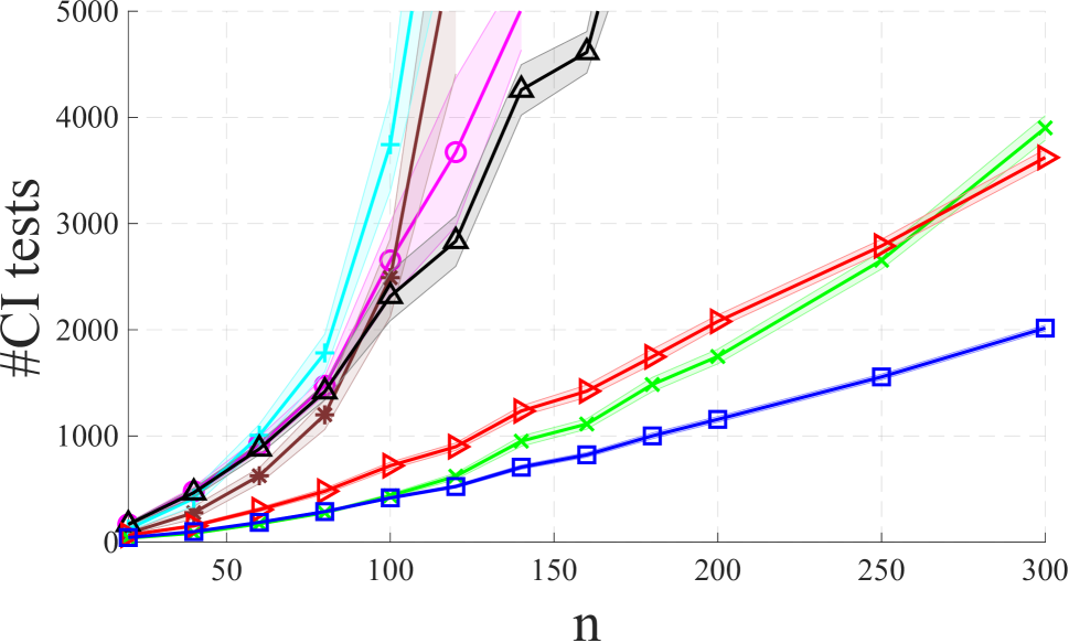
(a) Oracle; $p=n^{-0.82}$.

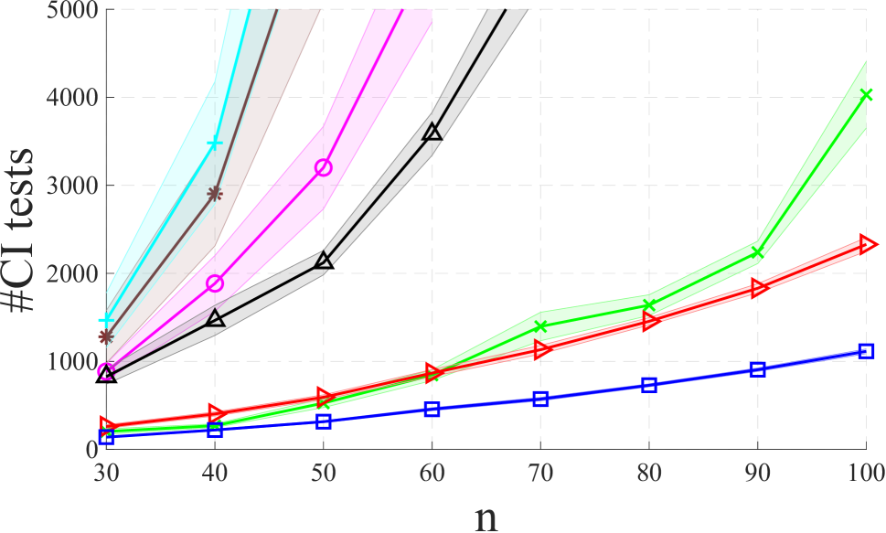
(b) Oracle; $p=n^{-0.72}$.

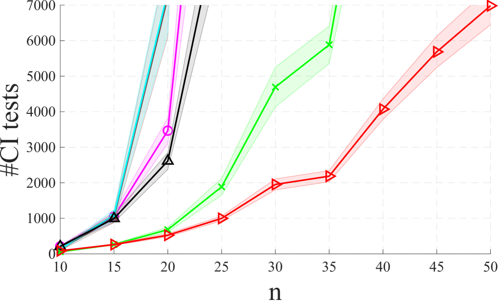
(c) Oracle; $p=n^{-0.53}$.

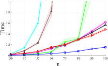
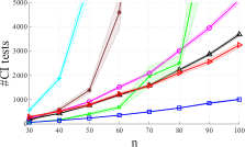
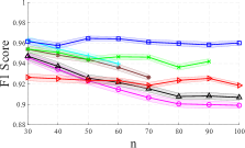
(d) On data; $G(n,p)$ with $p=n^{-0.72}$ and sample size = $50n$.

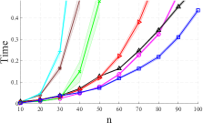
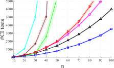
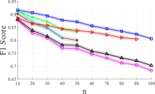
(e) On data; $G(n,p)$ with $p=n^{-0.65}$ and sample size = $20n$.

Figure 2: Performance of various algorithms on random graphs generated from Erdos-Renyi models.

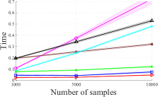
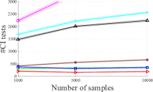
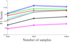
(a) On data; Diabetes ($n=104,|\mathbf{E}|=148,\omega=3,\Delta_{in}=2,\Delta=7,\alpha=12$, diamond-free).

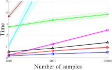
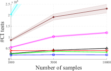
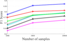
(b) On data; Andes ($n=223,|\mathbf{E}|=328,\omega=3,\Delta_{in}=6,\Delta=12,\alpha=23$, not diamond-free).

Figure 3: Performance of various algorithms on real-world structures.

In this section, we present a set of experiments to illustrate the effectiveness of our proposed algorithms. The MATLAB implementation of our algorithms is publicly available. We compare the performance of our algorithms, $RSL_{D}$ and RSL_ω with MARVEL (Mokhtarian et al. 2021), a modified version of PC (Spirtes et al. 2000; Pellet and Elisseeff 2008) that uses Mbs, GS (Margaritis and Thrun 1999), CS (Pellet and Elisseeff 2008), and MMPC (Tsamardinos, Aliferis, and Statnikov 2003b) on both real-world structures and Erdos-Renyi random graphs.

All aforementioned algorithms are Mb based. Thus, we initially use TC (Pellet and Elisseeff 2008) algorithm to compute $\textit{Mb}_{\mathbf{V}}$, and then pass it to each of the methods for the sake of fair comparison. The algorithms are compared in two settings: I) oracle, and II) finite sample. In the oracle setting, we are working in the population level, i.e., the CI tests are queried through an oracle that has access to the true CI relations among the variables. In the latter setting, algorithms have access to a dataset of finite samples from the true distribution. Hence, the CI tests might be noisy. The samples are generated using a linear model where each variable is a linear combination of its parents plus an exogenous noise variable; the coefficients are chosen uniformly at random from $[-1.5,-1]\cup[1,1.5]$, and the noises are generated from $\mathcal{N}(0,\sigma^{2})$, where $\sigma$ is selected uniformly at random from $[\sqrt{0.5},\sqrt{1.5}]$. As for the CI tests, we use Fisher Z-transformation (Fisher 1915) with significance level 0.01 in the algorithms (alternative values did not alter our experimental results) and $\frac{2}{n^{2}}$ for Mb discovery (Pellet and Elisseeff 2008). These are standard evaluations’ scenarios often performed in the structure learning literature (Colombo and Maathuis 2014; Améndola et al. 2020; Mokhtarian et al. 2021; Huang et al. 2012; Ghahramani and Beal 2001; Scutari, Vitolo, and Tucker 2019). We compare the algorithms in terms of runtime, the number of performed CI tests, and the f1-scores of the learned skeletons. In Appendix F, we further report other measurements (average size of conditioning sets, precision, recall, structural hamming distance) of the learned skeletons, and accuracy of the learned separating sets.

Figure 2 illustrates the performance of BN learning algorithms on random Erdos-Renyi $G(n,p)$ model graphs. Each point is reported as the average of 100 runs, and the shaded areas indicate the $80\%$ confidence intervals. Runtime and the number of CI tests are reported after Mb discovery. Figures 2(a), 2(b) and 2(c) demonstrate the number of CI tests each algorithm performed in the oracle setting, for the values of $p=n^{-0.82}$,$n^{-0.72}$, and $n^{-0.53}$, respectively. In 2(a), the graphs are diamond-free with high probability (see Section 7 for details). In 2(d), $\omega\leq 3$ with high probability, but the graphs are not necessarily diamond-free. In 2(c), $\omega\leq 4$, with high probability. We have not included the result of RSL_D in Figure 2(c), as the graphs contain diamonds with high probability, and RSL_D has no theoretical guarantee despite of low complexity. Figures 2(d) and 2(e) demonstrate the performance of the algorithms in the finite sample setting, when $50n$ and $20n$ samples were available, respectively. Although RSL_D does not have any theoretical correctness guarantee to recover the network (graphs are not diamond-free), both RSL_D and RSL_ω outperform other algorithms in terms of both accuracy and computational complexity in most cases. The lower runtime of MARVEL and MMPC compared to RSL_ω in Figure 2(e) can be explained through their significantly low accuracy due to skipping numerous CI tests.

Figure 3 illustrates the performance of BN learning algorithms on two real-world structures, namely Diabetes (Andreassen et al. 1991) and Andes (Conati et al. 1997) networks, over a range of different sample sizes. Each point is reported as the average of 10 runs. As seen in Figures 3(a) and 3(b), both RSL algorithms outperform other algorithms in both accuracy and complexity. Note that although Andes is not a diamond-free graph, RSL_D achieves the best accuracy in Figure 3(b). Similar experimental results for five real-world structures in both oracle and finite sample settings along with detailed information about these structures appear in Appendix F.

9 Conclusion

In this work, we presented the RSL algorithm for BN structure learning. Although our generic algorithm has exponential complexity, we showed that it could harness structural side information to learn the BN structure in polynomial time. In particular, we considered two types of side information about the underlying BN: I) when an upper bound on its clique number is known, and II) when the BN is diamond-free. We provided theoretical guarantees and upper bounds on the number of CI tests required by our algorithms. We demonstrated the superiority of our proposed algorithms in both synthetic and real-world structures. We showed in the experiments that even when the graph is not diamond-free, RSL_D outperforms various algorithms both in time complexity and accuracy.

Appendix

Table 3 summarizes how the Appendix is organized.

	Section	Title
	A	d-separation
	B	Technical proofs
	C	RSLD on networks with Diamonds
	D	Discussion on Algorithm 2
	E	Discussion on the implementation of RSL
	F	Reproducibility and additional experiments

Table 3: Organization of the Appendix.

Appendix A d-separation

Definition 5 (Path & Directed Path).

Let $X_{1},...,X_{m}$ be a set of distinct vertices in a DAG $\mathcal{G}=(\mathbf{V},\mathbf{E})$ such that $X_{i}\in\textit{N}_{\mathcal{G}}(X_{i+1})$. This is called a path between $X_{1}$ and $X_{m}$. When $X_{i}\in\textit{Pa}_{\mathcal{G}}(X_{i+1})$ for $1\leq i\leq m-1$, then we have a directed path from $X_{1}$ to $X_{m}$.

Definition 6 ($\textit{De}_{\mathcal{G}}(X)$).

Suppose $X,Y\in\mathbf{V}$ in a DAG $\mathcal{G}=(\mathbf{V},\mathbf{E})$. $Y$ is called a descendent of $X$ if there exists a directed path from $X$ to $Y$. We show by $\textit{De}_{\mathcal{G}}(X)$ the set of all descendants of $X$.

Definition 7 (Blocked).

A path between $X_{1}$ and $X_{m}$ is called blocked by a set S (with neither $X_{1}$ nor $X_{n}$ in S) whenever there is a node $X_{k}$, such that one of the following two possibilities holds:

1. $X_{k}\in\textbf{S}$ and $X_{k-1}\rightarrow X_{k}\rightarrow X_{k+1}$ or $X_{k-1}\leftarrow X_{k}\leftarrow X_{k+1}$ or $X_{k-1}\leftarrow X_{k}\rightarrow X_{k+1}$.

2. $X_{k-1}\rightarrow X_{k}\leftarrow X_{k+1}$ and neither $X_{k}$ nor any of its descendants is in S.

Definition 8 (d-separation).

Let $\textbf{X},\textbf{Y}$, and $\mathbf{S}$ be three disjoint subsets of vertices of a DAG $\mathcal{G}$. We say X and Y are d-separated by S, denoted by $\textbf{X}\perp_{\mathcal{G}}\textbf{Y}|\mathbf{S}$, if every path between vertices in X and Y is blocked by S.

Appendix B Technical proofs

To present the proofs, we need the following prerequisites.

Definition 9 (Collider).

Let $X_{1},...,X_{m}$ be a path between $X_{1}$ and $X_{m}$ in a DAG $\mathcal{G}=(\mathbf{V},\mathbf{E})$. A vertex $X_{j}$, $1<j<m$ on this path is called a collider if both $X_{j}\in\textit{Ch}_{\mathcal{G}}(X_{j+1})$ and $X_{j}\in\textit{Ch}_{\mathcal{G}}(X_{j-1})$. i.e., $X_{j-1}\rightarrow X_{j}\leftarrow X_{j+1}$.

Theorem 3 ((Mokhtarian et al. 2021)).

$X$ is removable in a DAG $\mathcal{G}$ if and only if the following two conditions are satisfied for every $W\in\textit{Ch}_{\mathcal{G}}(X).$

Condition 1: $\textit{N}_{\mathcal{G}}(X)\subseteq\textit{N}_{\mathcal{G}}(W)\cup\{W\}.$

Condition 2: $\textit{Pa}_{\mathcal{G}}(Y)\subseteq\textit{Pa}_{\mathcal{G}}(W)$ for any $Y\in\textit{Ch}_{\mathcal{G}}(X)\cap\textit{Pa}_{\mathcal{G}}(W)$.

Lemma 6 ((Mokhtarian et al. 2021)).

Suppose $\mathcal{G}=(\mathbf{V},\mathbf{E})$ is a perfect map of $P_{\mathbf{V}}$ and $X\in\mathbf{V}$ is a removable vertex in $\mathcal{G}$. In this case, $|\textit{Mb}_{\mathbf{V}}(X)|\leq\Delta_{\textit{in}}(\mathcal{G})$.

B.1 Proofs of Section 3:

Proposition 1.

Suppose $\mathcal{G}=(\mathbf{V},\mathbf{E})$ is a perfect map of $P_{\mathbf{V}}$. For each variable $X\in\mathbf{V}$, $\mathcal{G}[\mathbf{V}\setminus\{X\}]$ is a perfect map of $P_{\mathbf{V}\setminus\{X\}}$ if and only if $X$ is a removable vertex in $\mathcal{G}$.

Proof.

If part: We need to show that $\mathcal{G}[\mathbf{V}\setminus\{X\}]$ is an I-map and a D-map of $P_{\mathbf{V}\setminus\{X\}}$:

• I-map: Suppose $Y,Z\in\mathbf{V}\setminus\{X\}$ and $\mathbf{S}\subseteq\mathbf{V}\setminus\{X,Y,Z\}$ such that $Y\perp_{\mathcal{G}[\mathbf{V}\setminus\{X\}]}Z|\mathbf{S}$. Equation (1) implies $Y\perp_{\mathcal{G}}Z|\mathbf{S}$. Since $\mathcal{G}$ is an I-map of $P_{\mathbf{V}}$, $Y$ and $Z$ are independent conditioned on $\mathbf{S}$ in $P_{\mathbf{V}}$ and therefore in $P_{\mathbf{V}\setminus\{X\}}$. Hence, $\mathcal{G}[\mathbf{V}\setminus\{X\}]$ is an I-map of $P_{\mathbf{V}\setminus\{X\}}$.

• D-map: Suppose $Y,Z\in\mathbf{V}\setminus\{X\}$ and $\mathbf{S}\subseteq\mathbf{V}\setminus\{X,Y,Z\}$ such that $Y\centernot{\perp}_{\mathcal{G}[\mathbf{V}\setminus\{X\}]}Z|\mathbf{S}$. Equation (1) implies $Y\centernot{\perp}_{\mathcal{G}}Z|\mathbf{S}$. Since $\mathcal{G}$ is a D-map of $P_{\mathbf{V}}$, $Y$ and $Z$ are dependent conditioned on $\mathbf{S}$ in $P_{\mathbf{V}}$ and therefore in $P_{\mathbf{V}\setminus\{X\}}$. Hence, $\mathcal{G}[\mathbf{V}\setminus\{X\}]$ is a D-map of $P_{\mathbf{V}\setminus\{X\}}$.

Only if part: We need to prove that $X$ is removable in $\mathcal{G}$. Suppose $Y,Z\in\mathbf{V}\setminus\{X\}$ and $\mathbf{S}\subseteq\mathbf{V}\setminus\{X,Y,Z\}$. Since $\mathcal{G}[\mathbf{V}\setminus\{X\}]$ is a perfect map of $P_{\mathbf{V}\setminus\{X\}}$,

$$Y\perp_{\mathcal{G}[\mathbf{V}\setminus\{X\}]}Z|\mathbf{S}\iff Y\perp\mkern-9.5mu\perp_{P_{\mathbf{V}\setminus\{X\}}}Z|\mathbf{S}\iff Y\perp\mkern-9.5mu\perp_{P_{\mathbf{V}}}Z|\mathbf{S}.$$

Since $\mathcal{G}$ is a perfect map of $P_{\mathbf{V}}$, we obtain

$$Y\perp\mkern-9.5mu\perp_{P_{\mathbf{V}}}Z|\mathbf{S}\iff Y\perp_{\mathcal{G}[\mathbf{V}]}Z|\mathbf{S},$$

and consequently,

$$Y\perp_{\mathcal{G}[\mathbf{V}\setminus\{X\}]}Z|\mathbf{S}\iff Y\perp_{\mathcal{G}[\mathbf{V}]}Z|\mathbf{S}.$$

Therefore, due to the definition of removability (Definition 1), $X$ is a removable vertex in $\mathcal{G}$. ∎

Proposition 2.

Suppose $\mathcal{G}[\overline{\mathbf{V}}]$ is a perfect map of $P_{\overline{\mathbf{V}}}$ and $X$ is a removable variable in $\mathcal{G}[\overline{\mathbf{V}}]$. Algorithm 2 correctly finds $\textit{Mb}_{\overline{\mathbf{V}}\setminus\{X\}}$ by performing at most $\binom{|\textit{N}_{\mathcal{G}[\overline{\mathbf{V}}]}(X)|}{2}$ CI tests.

Proof.

Soundness: Suppose $X$ is a removable vertex in $\mathcal{G}[\overline{\mathbf{V}}]$ with the set of neighbors $\textit{N}_{\mathcal{G}[\overline{\mathbf{V}}]}(X)$. Since $\mathcal{G}[\overline{\mathbf{V}}]$ is a perfect map of $P_{\overline{\mathbf{V}}}$, Proposition 1 implies that $\mathcal{G}[\overline{\mathbf{V}}\setminus\{X\}]$ is a perfect map of $P_{{\overline{\mathbf{V}}}\setminus\{X\}}$. Hence, for any $Y\in\overline{\mathbf{V}}$,

$$\textit{Mb}_{\overline{\mathbf{V}}}(Y)=\textit{N}_{\mathcal{G}[\overline{\mathbf{V}}]}(Y)\cup\textit{CP}_{\mathcal{G}[\overline{\mathbf{V}}]}(Y),$$

and for any $Y\in\overline{\mathbf{V}}\setminus\{X\}$,

$$\textit{Mb}_{\overline{\mathbf{V}}\setminus\{X\}}(Y)=\textit{N}_{\mathcal{G}[\overline{\mathbf{V}}\setminus\{X\}]}(Y)\cup\textit{CP}_{\mathcal{G}[\overline{\mathbf{V}}\setminus\{X\}]}(Y).$$

First, note that for any $Y\in\overline{\mathbf{V}}\setminus\{X\}$,

$$\textit{N}_{\mathcal{G}[\overline{\mathbf{V}}\setminus\{X\}]}(Y)=\textit{N}_{\mathcal{G}[\overline{\mathbf{V}}]}(Y)\setminus\{X\},$$

and

$$\textit{CP}_{\mathcal{G}[\overline{\mathbf{V}}\setminus\{X\}]}(Y)\subseteq\textit{CP}_{\mathcal{G}[\overline{\mathbf{V}}]}(Y).$$

Algorithm 2 initializes $\textit{Mb}_{\overline{\mathbf{V}}\setminus\{X\}}$ with $\textit{Mb}_{\overline{\mathbf{V}}}$ in line 2, and remove $X$ from them in line 4. Hence, we only need to identify the variables in $D(Y):=\textit{CP}_{\mathcal{G}[\overline{\mathbf{V}}]}(Y)\setminus\textit{CP}_{\mathcal{G}[\overline{\mathbf{V}}\setminus\{X\}]}(Y)$ and remove them from $\textit{Mb}_{\overline{\mathbf{V}}\setminus\{X\}}(Y)$.

Suppose $Y\in\overline{\mathbf{V}}\setminus\{X\}$ such that $D(Y)\neq\varnothing$. Let $Z$ be a vertex in $D(Y)$. In this case, $Y$ and $Z$ have a common child in $\mathcal{G}[\overline{\mathbf{V}}]$, but do not have any common child in $\mathcal{G}[\overline{\mathbf{V}}\setminus\{X\}]$. Hence, $X$ is the only common child of $Y$ and $Z$ in $\mathcal{G}[\overline{\mathbf{V}}]$. However, this cannot happen if $X$ has a child in $\mathcal{G}[\overline{\mathbf{V}}]$, because if $W\in\textit{Ch}_{\mathcal{G}[\overline{\mathbf{V}}]}(X)$, Condition 1 of Theorem 3 implies that $Y,Z\in\textit{Pa}_{\mathcal{G}[\overline{\mathbf{V}}]}(W)$, i.e., $W$ is a common child for $Y,Z$ which is not possible. Hence,

$$\textit{Ch}_{\mathcal{G}[\overline{\mathbf{V}}]}(X)\neq\varnothing\Longrightarrow D(Y)=\varnothing,\,\hskip 5.0pt\forall Y\in\overline{\mathbf{V}}\setminus\{X\}.$$ (7)

In line 5 of Algorithm 2, if the condition $\textit{N}_{\mathcal{G}[\overline{\mathbf{V}}]}(X)=\textit{Mb}_{\overline{\mathbf{V}}}(X)$ does not hold, then $X$ has at least one co-parent, and therefore, at least one child. In this case, Equation (7) implies that Algorithm 2 correctly returns $\textit{Mb}_{\overline{\mathbf{V}}\setminus\{X\}}$.

As we mentioned above, if $Z\in D(Y)$, then $Y,Z\in\textit{Pa}_{\mathcal{G}[\overline{\mathbf{V}}]}(X)\subseteq\textit{N}_{\mathcal{G}[\overline{\mathbf{V}}]}(X)$. In the next step (lines 6-9), similar to the methods presented in (Mokhtarian et al. 2021) and (Margaritis and Thrun 1999), for all pairs $Y,Z\in\textit{N}_{\mathcal{G}[\overline{\mathbf{V}}]}(X)$ we can either perform $Y\perp\mkern-9.5mu\perp_{P_{\overline{\mathbf{V}}}}Z|\textit{Mb}_{\overline{\mathbf{V}}\setminus\{X\}}(Y)\setminus\{Y,Z\}$ or $Y\perp\mkern-9.5mu\perp_{P_{\overline{\mathbf{V}}}}Z|\textit{Mb}_{\overline{\mathbf{V}}\setminus\{X\}}(Z)\setminus\{Y,Z\}$ to decide whether they remain in each other’s Markov boundary after removing $X$ from $\mathcal{G}[\overline{\mathbf{V}}]$.

Complexity: The algorithm possibly performs CI tests only in line 7 for a pair of distinct variables in $\textit{N}_{\mathcal{G}[\overline{\mathbf{V}}]}(X)$. Hence, it perform at most $\binom{|\textit{N}_{\mathcal{G}[\overline{\mathbf{V}}]}(X)|}{2}$ CI tests. ∎

B.2 Proofs of Section 4:

We first present Lemma 7 that will be used for the proofs of this section.

Lemma 7.

Suppose $\mathcal{G}=(\overline{\mathbf{V}},\mathbf{E})$ is a DAG and a perfect map of $P_{\overline{\mathbf{V}}}$, $X\in\overline{\mathbf{V}}$, and $1\leq k\leq|\textit{Ch}_{\mathcal{G}}(X)|$ is a fixed number. If Equation (3) (or (9)) holds for all $\mathbf{S}\subseteq\textit{Mb}_{\overline{\mathbf{V}}}(X)$ with $\left|\mathbf{S}\right|\leq k-1$, then there exists $\mathbf{W}=\{W_{1},\dots,W_{k}\}\subseteq\textit{Ch}_{\mathcal{G}}(X)$ such that the following hold.

1. $W_{j}\in\textit{Pa}_{\mathcal{G}}(W_{i})$, for all $1\leq i<j\leq k$.

2. $Y\in\textit{Pa}_{\mathcal{G}}(W_{i})$, for all $1\leq i\leq k$ and $Y\in\textit{Mb}_{\overline{\mathbf{V}}}(X)\setminus\mathbf{W}$.

Proof.

We construct $\mathbf{W}$ iteratively, and for choosing $W_{1}$ we use Lemma 11 and Equation (11) that are presented in Appendix B.4. First note that for $|\mathbf{S}|=0$, Equation (9) reduces to Equation (11). Thus, Lemma 11 implies that there exists $W_{1}\in\textit{Ch}_{\mathcal{G}}(X)$ such that $\textit{Mb}_{\overline{\mathbf{V}}}(X)\cup\{X\}=\textit{Pa}_{\mathcal{G}}(W_{1})\cup\{W_{1}\}$. Hence, $\mathbf{W}=\{W_{1}\}$ satisfies the following conditions:

$$W_{j}\in\textit{Pa}_{\mathcal{G}}(W_{i}),\forall\>1\leq i<j\leq|\mathbf{W}|,$$ (8)

$$Y\in\textit{Pa}_{\mathcal{G}}(W_{i}),\forall\>1\leq i\leq|\mathbf{W}|\>\&\>Y\in\textit{Mb}_{\overline{\mathbf{V}}}(X)\setminus\mathbf{W}.$$

Now, suppose there exists $\mathbf{W}=\{W_{1},\dots,W_{m}\}\subseteq\textit{Ch}_{\mathcal{G}}(X)$ that satisfies Equation (8). In order to prove the lemma, it suffices to show that there exists a set $\mathbf{W^{{}^{\prime}}}$ with $|\mathbf{W^{{}^{\prime}}}|=m+1$ that satisfies Equation (8). To this end, we introduce $W_{m+1}\in\textit{Ch}_{\mathcal{G}}(X)\setminus\mathbf{W}$ such that $\mathbf{W^{{}^{\prime}}}=\mathbf{W}\cup\{W_{m+1}\}$ satisfies Equation (8).

Let $W_{m+1}$ be a variable in $\mathbf{A}:=\textit{Mb}_{\overline{\mathbf{V}}}(X)\setminus\mathbf{W}$ that does not have any descendants in $\mathbf{A}$. Note that $\mathbf{A}$ is non-empty since $m<|\textit{Ch}_{\mathcal{G}}(X)|$, and such a vertex exists due to the assumption that $\mathcal{G}$ is a DAG.

Claim 1: $W_{m+1}\in\textit{Ch}_{\mathcal{G}}(X)$.

proof of claim 1. As $m<|\textit{Ch}_{\mathcal{G}}(X)|$, $\mathbf{A}\cap\textit{Ch}_{\mathcal{G}}(X)\neq\varnothing$ and $W_{m+1}$ can be either a child or a co-parent of $X$ (parents of $X$ have at least one descendant in $\mathbf{A}$.) Assume by contradiction that $W_{m+1}\in\textit{CP}_{\mathcal{G}}(X)$. In this case, $W_{m+1}$ does not have any common child with $X$ other than the variables in $\mathbf{W}$, because $W_{m+1}$ does not have any descendants in $\mathbf{A}$.

Next, we will show that

$$X\perp_{\mathcal{G}}W_{m+1}|\textit{Mb}_{\overline{\mathbf{V}}}(X)\setminus(\{W_{m+1}\}\cup\mathbf{W}),$$

which is against Equation (9) for $\mathbf{S}=\mathbf{W}$ and $Y=W_{m+1}$. Therefore, $W_{m+1}\in\textit{Ch}_{\mathcal{G}}(X)$, i.e., claim 1 holds.

Suppose $\mathbf{B}:=\textit{Mb}_{\overline{\mathbf{V}}}(X)\setminus(\{W_{m+1}\}\cup\mathbf{W})$ and let $\mathcal{P}=(X,V_{1},\dots,V_{t},W_{m+1})$ be a path between $X$ and $W_{m+1}$. Note that $\mathcal{P}$ has length at least two since $X$ and $W_{m+1}$ are not neighbors. We have the following possibilities.

• $V_{1}\in\textit{Pa}_{\mathcal{G}}(X)$: $V_{1}$ blocks $\mathcal{P}$ since $V_{1}$ is not a collider on $\mathcal{P}$ and $V_{1}\in\mathbf{B}$.

• $V_{1}=W_{i}\in\mathbf{W}$: From the hypothesis of the previous iteration we have $W_{m+1}\in\textit{Pa}_{\mathcal{G}}(W_{i})$. Hence, $\mathcal{P}$ is not a directed path from $X$ to $W_{m+1}$ and has at least one collider. Let $Z$ be the collider on $\mathcal{P}$ closest to $X$. Hence, $Z\in\textit{De}_{\mathcal{G}}(W_{i})\cup\{W_{i}\}$, and neither $Z$ nor its descendants belongs to $\mathbf{B}$. Therefore, $Z$ blocks $\mathcal{P}$.

• $V_{1}\notin\mathbf{W}$, $V_{1}\in\textit{Ch}_{\mathcal{G}}(X)$, and $V_{1}$ is not a collider on $\mathcal{P}$: $V_{1}$ blocks $\mathcal{P}$ since $V_{1}\in\mathbf{B}$.

• $V_{1}\notin\mathbf{W}$, $V_{1}\in\textit{Ch}_{\mathcal{G}}(X)$, and $V_{1}$ is a collider on $\mathcal{P}$: As $W_{m+1}$ does not have any common child with $X$ other than the variables in $\mathbf{W}$, $\mathcal{P}$ has at least length 3 ($t\geq 2$). In this case, $V_{2}\neq W_{m+1}$ is a parent of $V_{1}$ and a co-parent of $X$. Thus, $V_{2}\in\mathbf{B}$. Therefore, $V_{2}$ blocks $\mathcal{P}$ as it cannot be a collider on $\mathcal{P}$.

We now show that the two properties of Equation (8) hold for $\mathbf{W}\cup\{W_{m+1}\}$. The first property directly follows from $W_{m+1}\in\textit{Mb}_{\overline{\mathbf{V}}}(X)\setminus\mathbf{W}$ and the definition of $\mathbf{W}$. To verify the second property, suppose $Y\in\textit{Mb}_{\overline{\mathbf{V}}}(X)\setminus(\mathbf{W}\cup\{W_{m+1}\})$. We need to show that $Y\in\textit{Pa}_{\mathcal{G}}(W_{m+1})$.

Let us define $\mathbf{C}:=(\textit{Mb}_{\overline{\mathbf{V}}}(X)\cup\{X\})\setminus(\{Y,W_{k+1}\}\cup\mathbf{W})$. We now show that $\mathbf{C}$ blocks all the paths of length at least two between $Y$ and $W_{m+1}$. Let $\mathcal{P}=(Y,V_{1},\dots,V_{t},W_{m+1})$ be a path of length at least two between $Y$ and $W_{m+1}$. If the last edge in this path is $V_{t}\to W_{m+1}$, $V_{t}$ blocks this path since it is not a collider and it is a member of $\mathbf{C}$. Now, suppose the last edge in this path is $V_{t}\leftarrow W_{m+1}$. Note that $Y\notin\textit{De}_{\mathcal{G}}(W_{m+1})$ by definition of $W_{m+1}$. Thus, there exists at least one collider on $\mathcal{P}$. Let $V_{i}$ be the closest collider of $\mathcal{P}$ to $W_{m+1}$. Since $V_{i}\in\textit{De}_{\mathcal{G}}(W_{m+1})$, neither $V_{i}$ nor any of its descendants appear in $\mathbf{C}$. Therefore, $V_{i}$ blocks $\mathcal{P}$. Hence, $\mathbf{C}$ blocks all the paths of length at least two between $Y$ and $W_{m+1}$. On the other hand, Equation (9) implies that

$$Y\centernot{\perp}_{\mathcal{G}}W_{m+1}|\mathbf{C}.$$

Hence, there must be a path of length one between $Y$ and $W_{m+1}$, i.e., $Y\in\textit{N}_{\mathcal{G}}(W_{m+1})$. $Y$ cannot be a child of $W_{m+1}$ by the definition of $W_{m+1}$, and therefore $Y\in\textit{Pa}_{\mathcal{G}}(W_{m+1})$. This completes the proof. ∎

Lemma 1.

Suppose $\mathcal{G}=(\overline{\mathbf{V}},\mathbf{E})$ is a DAG and a perfect map of $P_{\overline{\mathbf{V}}}$ such that $\omega(\mathcal{G})\leq m$. Vertex $X\in\overline{\mathbf{V}}$ is removable in $\mathcal{G}$ if for any $\mathbf{S}\subseteq\textit{Mb}_{\overline{\mathbf{V}}}(X)$ with $\left|\mathbf{S}\right|\leq m-2$, we have

$$Y\centernot{\perp\mkern-9.5mu\perp}_{P_{\overline{\mathbf{V}}}}Z|\big{(}\textit{Mb}_{\overline{\mathbf{V}}}(X)\cup\{X\}\big{)}\setminus\big{(}\{Y,Z\}\cup\mathbf{S}\big{)}, \forall Y,Z\in\textit{Mb}_{\overline{\mathbf{V}}}(X)\setminus\mathbf{S},$$ (9)

$$X\centernot{\perp\mkern-9.5mu\perp}_{P_{\overline{\mathbf{V}}}}Y|\textit{Mb}_{\overline{\mathbf{V}}}(X)\setminus(\{Y\}\cup\mathbf{S}), \forall Y\in\textit{Mb}_{\overline{\mathbf{V}}}(X)\setminus\mathbf{S}.$$

Furthermore, the set of vertices that satisfy Equation (9) is nonempty.

Proof.

First, we show that $|\textit{Ch}_{\mathcal{G}}(X)|\leq m-1$:

Assume by contradiction that $|\textit{Ch}_{\mathcal{G}}(X)|>m-1$. Lemma 7 for $k=m-1$ implies that there exists $\mathbf{W}\subseteq\textit{Ch}_{\mathcal{G}}(X)$ with $|\mathbf{W}|=m-1$ such that I) all the variables in $\mathbf{W}$ are neighbors, and II) each variable in $\textit{Mb}_{\overline{\mathbf{V}}}(X)\setminus\mathbf{W}$ is a parent of each of the variables in $\mathbf{W}$. Since $|\textit{Ch}_{\mathcal{G}}(X)|>m-1$, let $Z$ be a variable in $\textit{Ch}_{\mathcal{G}}(X)\setminus\mathbf{W}$. Hence, $\mathcal{G}[\mathbf{W}\cup\{X,Z\}]$ is a complete graph of size $m+1$ which is against the assumption that $\omega(\mathcal{G})\leq m$. Therefore, $|\textit{Ch}_{\mathcal{G}}(X)|\leq m-1$.

Now, Lemma 7 for $k=|\textit{Ch}_{\mathcal{G}}(X)|$ implies that there exists $\mathbf{W}\subseteq\textit{Ch}_{\mathcal{G}}(X)$ with $|\mathbf{W}|=|\textit{Ch}_{\mathcal{G}}(X)|$ such that I) all the variables in $\mathbf{W}$ are neighbors, and II) each variable in $\textit{Mb}_{\overline{\mathbf{V}}}(X)\setminus\mathbf{W}$ is a parent of each of the variables in $\mathbf{W}$. In this case, $\mathbf{W}$ must be equal to $\textit{Ch}_{\mathcal{G}}(X)$ which indicates that all the variables in $\textit{Mb}_{\overline{\mathbf{V}}}(X)\setminus\textit{Ch}_{\mathcal{G}}(X)$ are parents of the children of $X$ while the children of $X$ are neighbors of each other. Hence, Theorem 3 implies that $X$ is a removable variable in $\mathcal{G}$.

Finally, if $X$ has no child, Equation (9) holds. Also, there exists at least one vertex with no child in every DAG. Hence, the set of vertices that satisfy Equation (9) is nonempty. ∎

Proposition 3.

Suppose $\mathcal{G}[\overline{\mathbf{V}}]$ is a DAG and a perfect map of $P_{\overline{\mathbf{V}}}$ s.t. $\omega(\mathcal{G[\overline{\mathbf{V}}]})\leq m$. Algorithm 3 returns a removable vertex in $\mathcal{G}[\overline{\mathbf{V}}]$ by performing $\mathcal{O}(|\overline{\mathbf{V}}|\Delta_{\textit{in}}(\mathcal{G}[\overline{\mathbf{V}}])^{m})$ CI tests.

Proof.

The soundness of Algorithm 3 follows directly from Lemma 1.

Complexity: Suppose $X_{i^{*}}$ is the output of Algorithm 3. In this case, the algorithm has performed CI tests in line 5 to verify Equation (9) for $X_{1},\dots,X_{i^{*}}$. For each $1\leq j\leq i^{*}$, it performs at most

$$\sum_{s=0}^{m-2}\binom{|\textit{Mb}_{\overline{\mathbf{V}}}(X_{j})|}{s}[\binom{|\textit{Mb}_{\overline{\mathbf{V}}}(X_{j})|-s}{2}+|\textit{Mb}_{\overline{\mathbf{V}}}(X_{j})|-s]$$

CI tests. Since $X_{i^{*}}$ is removable in $\mathcal{G}[\overline{\mathbf{V}}]$, Lemma 6 implies that $|\textit{Mb}_{\overline{\mathbf{V}}}(X_{j})|\leq|\textit{Mb}_{\overline{\mathbf{V}}}(X_{i^{*}})|\leq\Delta_{\textit{in}}(\mathcal{G}[\overline{\mathbf{V}}])$. Hence, Algorithm 3 has performed

$$\mathcal{O}(i^{*}\sum_{s=0}^{m-2}\Delta_{\textit{in}}(\mathcal{G}[\overline{\mathbf{V}}])^{s+2})=\mathcal{O}(i^{*}\Delta_{\textit{in}}(\mathcal{G}[\overline{\mathbf{V}}])^{m})$$

CI tests. Note that $i^{*}\leq|\overline{\mathbf{V}}|$. ∎

Lemma 2.

Suppose $\mathcal{G}[\overline{\mathbf{V}}]$ is a DAG and a perfect map of $P_{\overline{\mathbf{V}}}$ with $\omega(\mathcal{G[\overline{\mathbf{V}}]})\leq m$. Let $X\in\overline{\mathbf{V}}$ be a vertex that satisfies Equation (3) and $Y\in\textit{Mb}_{\overline{\mathbf{V}}}(X)$. In this case, $Y\in\textit{CP}_{\mathcal{G}}(X)$ if and only if

$$\exists\mathbf{S}\subseteq\textit{Mb}_{\overline{\mathbf{V}}}(X)\setminus\{Y\}\!:\ \ \left|\mathbf{S}\right|=(m-1)\,,\ \ X\perp\mkern-9.5mu\perp_{P_{\overline{\mathbf{V}}}}Y|\textit{Mb}_{\overline{\mathbf{V}}}(X)\setminus(\{Y\}\cup\mathbf{S}).$$ (10)

Proof.

The if part is straightforward as $\textit{Mb}_{\overline{\mathbf{V}}}(X)=\textit{N}_{\mathcal{G}}(X)\cup\textit{CP}_{\mathcal{G}}(X)$.

only if part: As shown in the proof of Lemma 1, I) $|\textit{Ch}_{\mathcal{G}}(X)|\leq m-1$, II) children of $X$ are neighbors of each other, and III) each variable in $\textit{Mb}_{\overline{\mathbf{V}}}(X)\setminus\textit{Ch}_{\mathcal{G}}(X)$ is a parent of all the children of $X$.

We first show that if $Y\in\textit{CP}_{\mathcal{G}}(X)$, then

$$X\perp_{\mathcal{G}}Y|\textit{Mb}_{\overline{\mathbf{V}}}(X)\setminus(\{Y\}\cup\textit{Ch}_{\mathcal{G}}(X)).$$

Let $\mathcal{P}=(X,V_{1},\dots,V_{t},Y)$ be a path between $X$ and $Y$. If $V_{1}\in\textit{Pa}_{\mathcal{G}}(X)$, $V_{1}$ blocks $\mathcal{P}$ as it is not a collider on $\mathcal{P}$ and $V_{1}\in\textit{Mb}_{\overline{\mathbf{V}}}(X)\setminus(\{Y\}\cup\textit{Ch}_{\mathcal{G}}(X))$. Now, suppose $V_{1}\in\textit{Ch}_{\mathcal{G}}(X)$. Since $Y\in\textit{Pa}_{\mathcal{G}}(V_{1})$, $Y\notin\textit{De}_{\mathcal{G}}(V_{1})$ and $\mathcal{P}$ is not a directed path from $X$ to $Y$. Hence, $\mathcal{P}$ contains at least one collider. Let $Z$ be the collider on $\mathcal{P}$ closest to $V_{1}$. In this case, $Z\in\textit{De}_{\mathcal{G}}(V_{1})$. Hence, $Z$ blocks $\mathcal{P}$ since all the variables in $\textit{Mb}_{\overline{\mathbf{V}}}(X)\setminus(\{Y\}\cup\textit{Ch}_{\mathcal{G}}(X))$ are parents of $V_{1}$ and they cannot be a descendent of $Z$. Therefore, $\textit{Mb}_{\overline{\mathbf{V}}}(X)\setminus(\{Y\}\cup\textit{Ch}_{\mathcal{G}}(X))$ d-separates $X$ and $Y$.

On the other hand, if $\textit{CP}_{\mathcal{G}}(X)\neq\varnothing$ and $|\textit{Ch}_{\mathcal{G}}(X)|\leq m-2$, then Equation (3) with $\mathbf{S}=\textit{Ch}_{\mathcal{G}}(X)$ implies that $X\centernot{\perp\mkern-9.5mu\perp}_{P_{\overline{\mathbf{V}}}}Y|\textit{Mb}_{\overline{\mathbf{V}}}(X)\setminus(\{Y\}\cup\textit{Ch}_{\mathcal{G}}(X))$ which is against what we just proved. Hence, either $\textit{CP}_{\mathcal{G}}(X)=\varnothing$ or $|\textit{Ch}_{\mathcal{G}}(X)|=m-1$. In the first case, the claim is trivial, and for the second case, Equation (10) holds for $\mathbf{S}=\textit{Ch}_{\mathcal{G}}(X)$. ∎

Theorem 1.

Suppose $\mathcal{G}=(\mathbf{V},\mathbf{E})$ is a DAG and a perfect map of $P_{\mathbf{V}}$ with $\omega(\mathcal{G})\leq m$. Then, RSL (Algorithm 1) with sub-algorithms 3 and 4 is sound and complete, and performs $\mathcal{O}(|\mathbf{V}|^{2}\Delta_{\textit{in}}(\mathcal{G})^{m})$ CI tests.

Proof.

Soundness: Suppose $\mathcal{G}[\overline{\mathbf{V}}]$ is a perfect map of $P_{\overline{\mathbf{V}}}$ in a recursion. According to Proposition 3, FindRemovable function correctly finds a removable variable in $\mathcal{G}[\overline{\mathbf{V}}]$. Then, FindNeighbors function correctly finds $\textit{N}_{\mathcal{G}[\overline{\mathbf{V}}]}(X)$ and $\mathbfcal{S}_{X}$ according to Lemma 2. Then, UpdateMb function correctly updates $\textit{Mb}_{\overline{\mathbf{V}}\setminus\{X\}}$ according to Proposition 2. Hence, we call the RSL function for the next recursion with correct Markov boundaries. Moreover, Proposition 1 implies that $\mathcal{G}[\overline{\mathbf{V}}\setminus\{X\}]$ is a perfect map of $P_{\overline{\mathbf{V}}\setminus\{X\}}$. Therefore, as we initially assume that $\mathcal{G}$ is a perfect map of $P_{\mathbf{V}}$, $\mathcal{G}[\overline{\mathbf{V}}]$ is a perfect map of $P_{\overline{\mathbf{V}}}$ throughout all the recursions, and RSL correctly outputs $(\mathcal{H}[\overline{\mathbf{V}}],\,\mathbfcal{S}_{\overline{\mathbf{V}}})$.

Complexity: In each recursion, Lemma 6 implies that $|\textit{Mb}_{\overline{\mathbf{V}}}(X)|\leq\Delta_{\textit{in}}(\mathcal{G}[\overline{\mathbf{V}}])$. Hence, According to Propositions 2, 3 and Lemma 2, Algorithm 1 performs $\mathcal{O}(|\mathbf{V}|\Delta_{\textit{in}}(\mathcal{G})^{m})$ CI tests at each recursion. Therefore, it performs $\mathcal{O}(|\mathbf{V}|^{2}\Delta_{\textit{in}}(\mathcal{G})^{m})$ CI tests in total. ∎

B.3 Proofs of Section 5:

Proposition 4 (Verifiable).

Suppose $\mathcal{G}=(\mathbf{V},\mathbf{E})$ is a DAG with skeleton $\mathcal{H}$ that is a perfect map of $P_{\mathbf{V}}$. If the RSL with sub-algorithms 3 and 4, and input $m>0$ terminates, then the clique number of the learned skeleton is at least $\omega(\mathcal{G})$.

Proof.

To show this result, it suffices to prove that if an edge $e=\{X,Y\}$ belongs to $\mathcal{H}$, it also belongs to the output of RSL with $m>0$ and sub-algorithms 3 and 4.

Since $X$ and $Y$ are neighbors, then there exists no separating set for them in any subgraph $\mathcal{G}[\overline{\mathbf{V}}]$, where $X,Y\in\overline{\mathbf{V}}$. Hence, sub-algorithm 4 will not eliminate $Y$ from $\textit{N}_{\mathcal{G}[\overline{\mathbf{V}}]}(X)$ and vice versa. Furthermore, if $W$ is a removable vertex in $\mathcal{G}[\overline{\mathbf{V}}]$, function UpdateMB in Algorithm 2 will not remove $X$ and $Y$ from $\textit{Mb}_{\overline{\mathbf{V}}\setminus\{W\}}(Y)$ and $\textit{Mb}_{\overline{\mathbf{V}}\setminus\{W\}}(X)$, respectively. This ensures that RSL with any input $m>0$ will not remove the edge between $X$ and $Y$. ∎

B.4 Proofs of Section 6:

Lemma 3.

Suppose $\mathcal{G}=(\overline{\mathbf{V}},\mathbf{E})$ is a diamond-free DAG and a perfect map of $P_{\overline{\mathbf{V}}}$. Vertex $X\in\overline{\mathbf{V}}$ is removable in $\mathcal{G}$ if and only if

$$Y\centernot{\perp\mkern-9.5mu\perp}_{P_{\overline{\mathbf{V}}}}Z|(\textit{Mb}_{\overline{\mathbf{V}}}(X)\cup\{X\})\setminus\{Y,Z\},\ \ \ \ \forall Y,Z\in\textit{Mb}_{\overline{\mathbf{V}}}(X).$$ (11)

Furthermore, the set of removable vertices is nonempty.

Proof.

We first show in Lemma 11 that Equation (11) holds for a vertex $X$ if and only if

$$\exists W\in\textit{Ch}_{\mathcal{G}}(X)\cup\{X\}\ \ \text{such that}\ \ \textit{Mb}_{\overline{\mathbf{V}}}(X)\cup\{X\}=\textit{Pa}_{\mathcal{G}}(W)\cup\{W\}.$$ (12)

Afterwards, in lemmas 12 and 13, we show that in a diamond-free graph $\mathcal{G}$, vertex $X$ is removable if and only if (12) holds. This concludes the proof of Lemma 3.

To show that the set of removable variables is nonempty, we have that if $X$ has no children, then (5) holds. On the other hand, a DAG always contains a vertex with no children. Thus, the set of removable vertices of a diamond-free DAG is non-empty. ∎

Lemma 11.

Suppose $\mathcal{G}=(\overline{\mathbf{V}},\mathbf{E})$ is a DAG and a perfect map of $P_{\overline{\mathbf{V}}}$. Equation (11) holds for a vertex $X\in\overline{\mathbf{V}}$ if and only if there exists $W\in\textit{Ch}_{\mathcal{G}}(X)\cup\{X\}$, such that

$$\textit{Mb}_{\overline{\mathbf{V}}}(X)\cup\{X\}=\textit{Pa}_{\mathcal{G}}(W)\cup\{W\}.$$ (13)

Proof.

If part: Suppose $Y,Z\in\textit{Mb}_{\overline{\mathbf{V}}}(X)$ and $\mathbf{S}=\textit{Mb}_{\overline{\mathbf{V}}}(X)\cup\{X\}\setminus\{Y,Z\}$. We need to show that $Y\centernot{\perp}_{\mathcal{G}}Z|\mathbf{S}$. If either $W=Y$ or $W=Z$, then $Y$ and $Z$ are neighbors because of Equation (13), and therefore, they are not d-separable. Otherwise, $Y,Z\in\textit{Pa}_{\mathcal{G}}(W)$ and $W\in\mathbf{S}$. In this case, $Y\to W\leftarrow Z$ is an active path and $\mathbf{S}$ does not d-separate $Y$ and $Z$.

Only if part: Suppose $X\in\overline{\mathbf{V}}$ satisfies Equation (11). Take $W$ to be a vertex in $\textit{Ch}_{\mathcal{G}}(X)\cup\{X\}$ that has no nontrivial descendants in $\textit{Mb}_{\overline{\mathbf{V}}}(X)\cup\{X\}$. Note that such a vertex exists due to the acyclicity of $\mathcal{G}$. Since $W\in\textit{Ch}_{\mathcal{G}}(X)\cup\{X\}$, $\textit{Pa}_{\mathcal{G}}(W)\cup\{W\}\subseteq\textit{Mb}_{\overline{\mathbf{V}}}(X)\cup\{X\}$. It is enough to show that $\textit{Mb}_{\overline{\mathbf{V}}}(X)\cup\{X\}\subseteq\textit{Pa}_{\mathcal{G}}(W)\cup\{W\}$. Suppose $T\in\textit{Mb}_{\overline{\mathbf{V}}}(X)\setminus\{W\}$ and $\mathbf{S}=\textit{Mb}_{\overline{\mathbf{V}}}(X)\cup\{X\}\setminus\{T,W\}$. It suffices to show that $T\in\textit{Pa}_{\mathcal{G}}(W)$. We now show that $\mathbf{S}$ blocks all the paths of length at least two between $T$ and $W$. Let $\mathcal{P}=(T,V_{1},\dots,V_{k},W)$ be a path of length at least two between $T$ and $W$. If the last edge in this path is $V_{k}\to Z$, $V_{k}$ blocks this path since it is not a collider and it is a member of $\mathbf{S}$. Now suppose the last edge in this path is $V_{k}\leftarrow W$. Note that $T\notin\textit{De}_{\mathcal{G}}(W)$ by definition of $W$. Thus, there exists at least one collider on $\mathcal{P}$. Let $V_{i}$ be the closest collider of $\mathcal{P}$ to $W$. Since $V_{i}\in\textit{De}_{\mathcal{G}}(W)$, neither $V_{i}$ nor any of its descendants appear in $\mathbf{S}$. Therefore, $V_{i}$ blocks $\mathcal{P}$. Hence, $\mathbf{S}$ blocks all the paths of length at least two between $T$ and $W$. Since Equation (11) holds, there must be a path of length one between $T$ and $W$, i.e., $T\in\textit{N}_{\mathcal{G}}(W)$. $T$ cannot be a child of $W$ by definition of $W$, and therefore $T\in\textit{Pa}_{\mathcal{G}}(W)$. ∎

Lemma 12.

Suppose $\mathcal{G}=(\overline{\mathbf{V}},\mathbf{E})$ is a DAG and a perfect map of $P_{\overline{\mathbf{V}}}$, and $X\in\overline{\mathbf{V}}$ is a removable variable in $\mathcal{G}$. There exists a variable $W\in\textit{Ch}_{\mathcal{G}}(X)\cup\{X\}$ such that Equation (13) holds.

Proof.

Take $W$ as a vertex in $\textit{Ch}_{\mathcal{G}}(X)\cup\{X\}$ that has no children in $\textit{Mb}_{\overline{\mathbf{V}}}(X)\cup\{X\}$. Note that such a vertex exists due to acyclicity. We will show Equation (13) holds for this $W$.

If $W=X$, then the claim is trivial as $X$ has no children and $\textit{Mb}_{\overline{\mathbf{V}}}(X)=\textit{Pa}_{\mathcal{G}}(X)$. Otherwise, $W\in\textit{Ch}_{\mathcal{G}}(X)$. Hence, $\textit{Pa}_{\mathcal{G}}(W)\cup\{W\}\subseteq\textit{Mb}_{\overline{\mathbf{V}}}(X)\cup\{X\}$. Now take an arbitrary vertex $T\in\textit{Mb}_{\overline{\mathbf{V}}}(X)\setminus\{W\}$. It suffices to show that $T\in\textit{Pa}_{\mathcal{G}}(W)$.

If $T\in\textit{N}_{\mathcal{G}}(X)\setminus\{W\}$, according to Condition 1 of removability (Theorem 3), all of the neighbors of $X$ are adjacent to the children of $X$. Hence, $T$ and $W$ are neighbors. Since $W$ has no children in $\textit{Mb}_{\overline{\mathbf{V}}}(X)\cup\{X\}$, $T\in\textit{Pa}_{\mathcal{G}}(W)$.

If $T\in\textit{CP}_{\mathcal{G}}(X)$, then $X$ and $T$ have at least a common child $Y$. If $Y=W$, then $W\in\textit{Pa}_{\mathcal{G}}(Z)$. Otherwise, $Y\in\textit{Ch}_{\mathcal{G}}(X)\setminus\{W\}$. As we showed in the previous case, $Y$ is a parent of $W$, and therefore, $Y\in\textit{Ch}_{\mathcal{G}}(X)\cap\textit{Pa}_{\mathcal{G}}(W)$. Hence, Condition 2 of Theorem 3 implies that $T\in\textit{Pa}_{\mathcal{G}}(W)$, which completes the proof. ∎

Lemma 13.

Suppose $\mathcal{G}=(\overline{\mathbf{V}},\mathbf{E})$ is a diamond-free DAG and a perfect map of $P_{\overline{\mathbf{V}}}$. $X\in\overline{\mathbf{V}}$ is removable in $\mathcal{G}$ if there exists $W\in\textit{Ch}_{\mathcal{G}}(X)\cup\{X\}$ such that $\textit{Mb}_{\overline{\mathbf{V}}}(X)\cup\{X\}=\textit{Pa}_{\mathcal{G}}(W)\cup\{W\}$.

Proof.

In order to prove the removability of $X$ in $\mathcal{G}$, we show that the conditions of Theorem 3 are satisfied. Take an arbitrary $W^{\prime}\in\textit{Ch}_{\mathcal{G}}(X)$. If $W^{\prime}=W$, both conditions are satisfied as all vertices in $\textit{Mb}_{\overline{\mathbf{V}}}(X)$ are parents of $W^{\prime}$. Now suppose $W^{\prime}\in\textit{Ch}_{\mathcal{G}}(X)\setminus\{W\}$. In this case, $W^{\prime}\in\textit{Pa}_{\mathcal{G}}(W)$.

Condition 1: Suppose $Y\in\textit{N}_{\mathcal{G}}(X)$. We need to show that $Y$ and $W^{\prime}$ are neighbors. Consider the induced subgraph $\mathcal{G}[\{X,W,W^{\prime},Y\}]$, where we have $X,W^{\prime},Y\in\textit{Pa}_{\mathcal{G}}(W)$, $X\in\textit{Pa}_{\mathcal{G}}(W^{\prime})$ and $X\in\textit{N}_{\mathcal{G}}(Y)$. Since $\mathcal{G}$ is diamond-free, $W^{\prime}$ and $Y$ must be neighbors.

Condition 2: Suppose $Y\in\textit{Ch}_{\mathcal{G}}(X)\cap\textit{Pa}_{\mathcal{G}}(W^{\prime})$, and $T\in\textit{Pa}_{\mathcal{G}}(Y)$. We need to show that $T\in\textit{Pa}_{\mathcal{G}}(W^{\prime})$. Now, consider the induced subgraph $\mathcal{G}[\{T,Y,W^{\prime},W\}]$, where we have $T,Y,W^{\prime}\in\textit{Pa}_{\mathcal{G}}(W)$, $T\in\textit{Pa}_{\mathcal{G}}(Y)$ and $Y\in\textit{Pa}_{\mathcal{G}}(W^{\prime})$. Since $\mathcal{G}$ is diamond-free, $T$ and $W^{\prime}$ must be neighbors, which implies that $T\in\textit{Pa}_{\mathcal{G}}(W^{\prime})$ due to acyclicity of $\mathcal{G}$. ∎

Proposition 5.

Suppose $\mathcal{G}[\overline{\mathbf{V}}]$ is a diamond-free DAG and a perfect map of $P_{\overline{\mathbf{V}}}$. FindRemovable returns a removable vertex in $\mathcal{G}[\overline{\mathbf{V}}]$ by performing at most $|\overline{\mathbf{V}}|\binom{\Delta_{\textit{in}}(\mathcal{G}[\overline{\mathbf{V}}])}{2}$ CI tests.

Proof.

Soundness: $\mathcal{G}[\overline{\mathbf{V}}]$ is a diamond-free graph and a perfect map of $P_{\overline{\mathbf{V}}}$. Hence, Lemma 3 implies that I) $\mathcal{G}[\overline{\mathbf{V}}]$ has at least one removable vertex, and II) Equation (5) holds for $X_{i}\in\overline{\mathbf{V}}$ if and only if $X_{i}$ is removable in $\mathcal{G}[\overline{\mathbf{V}}]$. Therefore, the output of FindRemovable function is a removable vertex.

Complexity: Suppose $X_{i^{*}}$ is the output of FindRemovable. In this case, the function has performed CI tests in line 5 to verify Equation (5) for $X_{1},\dots,X_{i^{*}}$. For each $1\leq j\leq i^{*}$, it performs at most $\binom{|\textit{Mb}_{\overline{\mathbf{V}}}(X_{j})|}{2}$ CI tests. Since $X_{i^{*}}$ is removable in $\mathcal{G}[\overline{\mathbf{V}}]$, Lemma 6 implies that $|\textit{Mb}_{\overline{\mathbf{V}}}(X_{j})|\leq|\textit{Mb}_{\overline{\mathbf{V}}}(X_{i^{*}})|\leq\Delta_{\textit{in}}(\mathcal{G}[\overline{\mathbf{V}}])$. Hence, FindRemovable has performed at most $i^{*}\binom{\Delta_{\textit{in}}(\mathcal{G}[\overline{\mathbf{V}}])}{2}$ CI tests. Note that $i^{*}\leq|\overline{\mathbf{V}}|$. ∎

Lemma 4.

Suppose $\mathcal{G}=(\overline{\mathbf{V}},\mathbf{E})$ is a diamond-free DAG and a perfect map of $P_{\overline{\mathbf{V}}}$. Let $X\in\overline{\mathbf{V}}$ be a removable vertex in $\mathcal{G}$, and $Y\in\textit{Mb}_{\overline{\mathbf{V}}}(X)$. In this case, $Y\in\textit{CP}_{\mathcal{G}}(X)$ if and only if

$$\exists Z\in\textit{Mb}_{\overline{\mathbf{V}}}(X)\setminus\{Y\}\!:\ \ X\perp\mkern-9.5mu\perp_{P_{\overline{\mathbf{V}}}}Y|\textit{Mb}_{\overline{\mathbf{V}}}(X)\setminus\{Y,Z\}.$$ (14)

Proof.

If part: Since $\mathcal{G}$ is a perfect map of $P_{\overline{\mathbf{V}}}$,

$$\textit{Mb}_{\overline{\mathbf{V}}}(X)=\textit{N}_{\mathcal{G}}(X)\cup\textit{CP}_{\mathcal{G}}(X).$$

Equation (14) implies that $X$ and $Y$ are d-separable. Hence, they are not neighbors and $Y\in\textit{CP}_{\mathcal{G}}(X)$.

Only if part: Since $\mathcal{G}$ is a perfect map of $P_{\overline{\mathbf{V}}}$ and $X$ is a removable variable in $\mathcal{G}$, Lemma 12 implies that there exists a variable $Z\in\textit{Ch}_{\mathcal{G}}(X)\cup\{X\}$ such that

$$\textit{Mb}_{\overline{\mathbf{V}}}(X)\cup\{X\}=\textit{Pa}_{\mathcal{G}}(Z)\cup\{Z\}.$$ (15)

We will show that Equation (14) holds for this $Z$.

We first show that if $Z\neq X$, then $Z$ is the only common child of $X$ and $Y$: Assume by contradiction that $W\neq Z$ is a common child of $X$ and $Y$. Since $W\in\textit{Mb}_{\overline{\mathbf{V}}}(X)\cup\{X\}$, $W$ is a parent of $Z$. Therefore, $\mathcal{G}[\{X,W,Y,Z\}]$ is a diamond graph which is against our assumption.

Now, we need to prove that $\mathbf{S}=\textit{Mb}_{\overline{\mathbf{V}}}(X)\setminus\{Y,Z\}$ d-separates $X$ and $Y$, i.e., blocks all the paths between them. Let $\mathcal{P}=(X,V_{1},\dots,V_{k},Y)$ be a path between $X$ and $Y$. Note that $\mathcal{P}$ has length at least two since $X$ and $Y$ are not neighbors. We have the following possibilities.

• $V_{1}\in\textit{Pa}_{\mathcal{G}}(X)$: $V_{1}$ blocks $\mathcal{P}$ since $V_{1}$ is not a collider on $\mathcal{P}$ and $V_{1}\in\mathbf{S}$.

• $V_{1}=Z$: In this case, $Z\in\textit{Ch}_{\mathcal{G}}(X)$ as $Z\neq X$. Since $Y\in\textit{Mb}_{\overline{\mathbf{V}}}(X)\setminus\{Z\}\subset\textit{Pa}_{\mathcal{G}}(Z)$, $\mathcal{P}$ is not a directed path from $X$ to $Y$ and has at least one collider. Let $W$ be the collider on $\mathcal{P}$ closest to $X$. Hence, $W\in\textit{De}_{\mathcal{G}}(Z)\cup\{Z\}$, and neither $W$ nor its descendants belongs to $\mathbf{S}$. Therefore, $W$ blocks $\mathcal{P}$.

• $V_{1}\neq Z$, $V_{1}\in\textit{Ch}_{\mathcal{G}}(X)$, and $V_{1}$ is not a collider on $\mathcal{P}$: $V_{1}$ blocks $\mathcal{P}$ since $V_{1}\in\mathbf{S}$.

• $V_{1}\neq Z$, $V_{1}\in\textit{Ch}_{\mathcal{G}}(X)$, and $V_{1}$ is a collider on $\mathcal{P}$: Since $\textit{Ch}_{\mathcal{G}}(X)\neq\varnothing$, $Z\neq X$, and $Z$ is the only common child of $X$ and $Y$. Hence, $\mathcal{P}$ has at least length 3 ($k\geq 2$). In this case, $V_{2}\neq Y$ is a parent of $V_{1}$ and a co-parent of $X$. Thus, $V_{2}\in\mathbf{S}$. Therefore, $V_{2}$ blocks $\mathcal{P}$ as it cannot be a collider on $\mathcal{P}$.

In all the cases, $\mathbf{S}$ blocks $\mathcal{P}$, and therefore, d-separates $X$ and $Y$. ∎

In order to prove Theorem 2, we first show the following result.

Lemma 15.

Suppose $\mathcal{G}[\overline{\mathbf{V}}]$ is a diamond-free DAG and a perfect map of $P_{\overline{\mathbf{V}}}$. If $X$ is removable in $\mathcal{G}[\overline{\mathbf{V}}]$, then FindNeighbors function for learning $\textit{N}_{\mathcal{G}[\overline{\mathbf{V}}]}(X)$ and $\mathbfcal{S}_{X}$ is sound, and performs $\mathcal{O}(\Delta_{\textit{in}}(\mathcal{G}[\overline{\mathbf{V}}])^{2})$ number of CI tests.

Proof.

Soundness: According to the definition of Markov boundary, for every $Y\in\overline{\mathbf{V}}\setminus\textit{Mb}_{\overline{\mathbf{V}}}(X)$,

$$X\perp\mkern-9.5mu\perp_{P_{\overline{\mathbf{V}}}}Y|\textit{Mb}_{\overline{\mathbf{V}}}(X).$$

Since $\mathcal{G}[\overline{\mathbf{V}}]$ is a perfect map of $P_{\overline{\mathbf{V}}}$,

$$X\perp\mkern-9.5mu\perp_{P_{\overline{\mathbf{V}}}}Y|\textit{Mb}_{\overline{\mathbf{V}}}(X)\iff X\perp_{\mathcal{G}[\overline{\mathbf{V}}]}Y|\textit{Mb}_{\overline{\mathbf{V}}}(X).$$

Therefore, line 3 of Algorithm 4 correctly finds a separating set for $X$ and the variables in $\overline{\mathbf{V}}\setminus\textit{Mb}_{\overline{\mathbf{V}}}(X)$.

Since $\mathcal{G}[\overline{\mathbf{V}}]$ is a perfect map of $P_{\overline{\mathbf{V}}}$, Equation (2) implies that

$$\textit{Mb}_{\overline{\mathbf{V}}}(X)=\textit{N}_{\mathcal{G}[\overline{\mathbf{V}}]}(X)\cup\textit{CP}_{\mathcal{G}[\overline{\mathbf{V}}]}(X).$$

For every $Y\in\textit{Mb}_{\overline{\mathbf{V}}}(X)$, Algorithm 4 checks whether Equation (6) holds for $Y$. If Equation (6) holds for $Y,$ Lemma 4 implies that $Y\in\textit{CP}_{\mathcal{G}[\overline{\mathbf{V}}]}(X)$ and $\textit{Mb}_{\mathcal{G}[\overline{\mathbf{V}}]}(X)\setminus\{Y,Z\}$ is a separating set for $X$ and $Y.$ Otherwise, it implies that $Y\in\textit{N}_{\mathcal{G}[\overline{\mathbf{V}}]}(X)$. Hence, Algorithm 4 correctly finds a separating set for $X$ and $\textit{CP}_{\mathcal{G}[\overline{\mathbf{V}}]}(X)$ in line 6 and correctly identifies $\textit{N}_{\mathcal{G}[\overline{\mathbf{V}}]}(X)$ in line 8.

Complexity: Algorithm 4 performs at most $|\textit{Mb}_{\overline{\mathbf{V}}}(X)|-1$ CI tests in line 5 to check Equation (6) for each $Y\in\textit{Mb}_{\overline{\mathbf{V}}}(X)$. Since $X$ is removable in $\mathcal{G}[\overline{\mathbf{V}}]$, Lemma 6 implies that $|\textit{Mb}_{\overline{\mathbf{V}}}(X)|\leq\Delta_{\textit{in}}(\mathcal{G}[\overline{\mathbf{V}}])$. Thus, Algorithm 4 performs $\mathcal{O}(\Delta_{\textit{in}}(\mathcal{G}[\overline{\mathbf{V}}])^{2})$ CI tests. ∎

Theorem 2.

Suppose $\mathcal{G}=(\mathbf{V},\mathbf{E})$ is a diamond-free DAG and a perfect map of $P_{\mathbf{V}}$. RSL_D is sound and complete, and performs $\mathcal{O}(|\mathbf{V}|^{2}\Delta_{\textit{in}}(\mathcal{G})^{2})$ CI tests.

Proof.

Soundness: Suppose $\mathcal{G}[\overline{\mathbf{V}}]$ is a perfect map of $P_{\overline{\mathbf{V}}}$ in a recursion. According to Proposition 5, FindRemovable function correctly finds a removable variable in $\mathcal{G}[\overline{\mathbf{V}}]$. Then, FindNeighbors function correctly finds $\textit{N}_{\mathcal{G}[\overline{\mathbf{V}}]}(X)$ and $\mathbfcal{S}_{X}$ according to Lemma 15. Then, UpdateMb function correctly updates $\textit{Mb}_{\overline{\mathbf{V}}\setminus\{X\}}$ according to Proposition 2. Hence, we call the RSL function for the next recursion with correct Markov boundaries. Moreover, Proposition 1 implies that $\mathcal{G}[\overline{\mathbf{V}}\setminus\{X\}]$ is a perfect map of $P_{\overline{\mathbf{V}}\setminus\{X\}}$. Therefore, as we initially assume that $\mathcal{G}$ is a perfect map of $P_{\mathbf{V}}$, $\mathcal{G}[\overline{\mathbf{V}}]$ is a perfect map of $P_{\overline{\mathbf{V}}}$ throughout all the recursions, and RSL correctly outputs $(\mathcal{H}[\overline{\mathbf{V}}],\,\mathbfcal{S}_{\overline{\mathbf{V}}})$.

Complexity: In each recursion, Lemma 6 implies that $|\textit{Mb}_{\overline{\mathbf{V}}}(X)|\leq\Delta_{\textit{in}}(\mathcal{G}[\overline{\mathbf{V}}])$. Hence, According to Propositions 2, 5 and Lemma 15, Algorithm 1 performs $\mathcal{O}(|\mathbf{V}|\Delta_{\textit{in}}(\mathcal{G})^{2})$ CI tests at each recursion. Therefore, it performs $\mathcal{O}(|\mathbf{V}|^{2}\Delta_{\textit{in}}(\mathcal{G})^{2})$ CI tests in total. ∎

B.5 Proofs of Section 7:

Lemma 5.

A random graph $\mathcal{G}$ generated from Erdos-Renyi model $G(n,p)$ is diamond-free with high probability when $pn^{0.8}\!\rightarrow\!0$ and $\omega(\mathcal{G})\leq m$ when $pn^{2/m}\!\rightarrow\!0$.

Proof.

From the theory of random graphs (Gilbert 1959), we know that any fixed graph $\mathcal{G}^{\prime}$, with $n_{\mathcal{G}^{\prime}}$ vertices and $e_{\mathcal{G}^{\prime}}$ edges does not appear in an Erdos-Renyi graph $G(n,p)$ with high probability as long as $pn^{1/f(\mathcal{G}^{\prime})}\!\rightarrow\!0$, as $n\!\rightarrow\!\infty$, where $f(\mathcal{G}^{\prime})\!:=\!\max\{e_{\mathcal{K}}/n_{\mathcal{K}}:\mathcal{K}\subseteq\mathcal{G}^{\prime}\}$. This implies that the realizations of $G(n,p)$ are diamond-free with high probability when $pn^{0.8}\!\rightarrow\!0$ and their clique numbers are bounded by $m$ when $pn^{2/m}\!\rightarrow\!0$. ∎

Appendix C RSL_D on networks with diamonds

(a) The true DAG

(b) Learned essential graph when $D$ is removed first

(c) Learned essential graph when $A$ is removed first

Figure 4: $RSL_{D}$ on networks including diamonds.

In this section, we discuss how $RSL_{D}$ performs on graphs including diamonds. Consider the DAG in Figure 4(a), which is one of the forbidden structures in Figure 1. All vertices $A,B,C$ and $D$ satisfy the conditions of Equation (5), and all of them have a Markov boundary of size 3. As a result, $RSL_{D}$ will randomly choose one of them as the first removable node and continue with the remaining structure. However, the vertex $A$ is not removable according to Definition 1. As a result, if $RSL_{D}$ removes one of $B,C$, or $D$ first, it will recover the true essential graph depicted in Figure 4(b). On the other hand, if $RSL_{D}$ removes $A$ first, an erroneous extra edge between the vertices $B$ and $C$ will appear in the output structure, as depicted in red in Figure 4(c). Although $RSL_{D}$ can make errors in recovering the BNs with diamonds as in this example, the next proposition shows that $RSL_{D}$ can only infer extra edges, i.e., the recall of $RSL_{D}$ is always equal to one, even if the true BN includes diamonds.

Proposition 11.

If RSL_D terminates, the recovered BN structure contains no false negative edges.

Proof.

Suppose the true BN is the DAG $\mathcal{G}=(\mathbf{V},\mathbf{E})$, and $\hat{\mathcal{G}}$ is the graph structure recovered from the output of $RSL_{D}$. It suffices to prove every edge in $\mathcal{G}$ also exists in $\hat{\mathcal{G}}$. Take an arbitrary edge $(X,Y)\in\mathbf{E}$. Since $X$ and $Y$ are neighbors, $X$ and $Y$ are in each other’s Markov boundary at the beginning. Throughout $RSL_{D}$, Markov boundaries are only updated through Algorithm 2, where vertices $X$ and $Y$ are removed from each other’s Markov boundary if either a separating set for them is found, or one of them is removed. Since $X$ and $Y$ are neighbors, no separating set for them exists. As a result, as long as none of $X$ and $Y$ are removed, they stay in each other’s Mb. Suppose without loss of generality that $X$ is removed first, where the set of remaining variables is $\overline{\mathbf{V}}$. Since $Y$ is still in $\textit{Mb}_{\overline{\mathbf{V}}}(X)$, and no separating set exists for $X$ and $Y$ (Equation 6 does not hold for any $Z$), function FindNeighbors adds $Y$ to $N_{\mathcal{G}[\overline{\mathbf{V}}]}(X)$ in line 8. Therefore, $X$ and $Y$ are neighbors in the output of $RSL_{D}$, and $\hat{\mathcal{G}}$, which completes the proof. ∎

Based on Proposition 11, we propose the following implementation of FindRemovable for $RSL_{D}$, which does not require the diamond-freeness of the true BN, and yet guarantees a recall of 1. If no removable vertex is found at the end of for loop of line 4 of function FindRemovable, return the node with the smallest Mb size. If the true BN is diamond-free, this will not affect the algorithm as there always exists a vertex that satisfies Equation (5) according to Lemma 3. Otherwise, i.e., if the true BN contains diamonds, this implementation ensures that $RSL_{D}$ never gets stuck, and from Proposition 11 it has no false negatives in its output. Note that $RSL_{D}$ might still recover the true BN if it has diamonds.

Appendix D Discussion on Algorithm 2

Algorithm 2 takes as input a removable variable $X$ in $\mathcal{G}[\overline{\mathbf{V}}]$ with its set of neighbors $\textit{N}_{\mathcal{G}[\overline{\mathbf{V}}]}(X)$, and the set of Markov boundaries $\textit{Mb}_{\overline{\mathbf{V}}}$. The output of the algorithm is the set of Markov boundaries after removing $X$ from $\mathcal{G}[\overline{\mathbf{V}}]$, i.e., $\textit{Mb}_{\overline{\mathbf{V}}\setminus\{X\}}$. See the proof of Proposition 2 for more details.

Function UpdateMb initializes $\textit{Mb}_{\overline{\mathbf{V}}\setminus\{X\}}(Y)$ with $\textit{Mb}_{\overline{\mathbf{V}}}(Y)$ and then removes the extra variables as follows. Since $X$ is removable in $\mathcal{G}[\overline{\mathbf{V}}]$, for any $Y\in\overline{\mathbf{V}}\setminus\{X\}$,

$$\textit{Mb}_{\overline{\mathbf{V}}}(Y)=\textit{N}_{\mathcal{G}[\overline{\mathbf{V}}]}(Y)\cup\textit{CP}_{\mathcal{G}[\overline{\mathbf{V}}]}(Y),$$ (16)

$$\textit{Mb}_{\overline{\mathbf{V}}\setminus\{X\}}(Y)=\textit{N}_{\mathcal{G}[\overline{\mathbf{V}}\setminus\{X\}]}(Y)\cup\textit{CP}_{\mathcal{G}[\overline{\mathbf{V}}\setminus\{X\}]}(Y).$$

First, note that $\textit{N}_{\mathcal{G}[\overline{\mathbf{V}}\setminus\{X\}]}(Y)\subseteq\textit{N}_{\mathcal{G}[\overline{\mathbf{V}}]}(Y)$ and $\textit{CP}_{\mathcal{G}[\overline{\mathbf{V}}\setminus\{X\}]}(Y)\subseteq\textit{CP}_{\mathcal{G}[\overline{\mathbf{V}}]}(Y)$. We define

$$D_{1}(Y):=\textit{N}_{\mathcal{G}[\overline{\mathbf{V}}]}(Y)\setminus\textit{N}_{\mathcal{G}[\overline{\mathbf{V}}\setminus\{X\}]}(Y),\text{ and }$$ (17)

$$D_{2}(Y):=\textit{CP}_{\mathcal{G}[\overline{\mathbf{V}}]}(Y)\setminus\textit{CP}_{\mathcal{G}[\overline{\mathbf{V}}\setminus\{X\}]}(Y).$$

One can see that $D_{1}(Y)$ is empty for $Y\in\overline{\mathbf{V}}\setminus(\textit{Mb}_{\overline{\mathbf{V}}}(X)\cup\{X\})$, and is $\{X\}$ for $Y\in\textit{Mb}_{\overline{\mathbf{V}}}(X)$. Hence, Algorithm 2 removes $X$ from $\textit{Mb}_{\overline{\mathbf{V}}}(Y)$ when $Y\in\textit{Mb}_{\overline{\mathbf{V}}}(X)$ in line 4.

The algorithm identifies the rest of the extra variables in lines 5-9 which are the variables in $D_{2}(Y)$. We show in the proof Proposition 2 that if $X$ has at least one child, then $D_{2}(Y)$ is empty for all $Y\in\overline{\mathbf{V}}\setminus\{X\}$. In line 5 of Algorithm 2, if the condition $\textit{N}_{\mathcal{G}[\overline{\mathbf{V}}]}(X)=\textit{Mb}_{\overline{\mathbf{V}}}(X)$ does not hold, then $X$ has at least one co-parent, and therefore, at least one child. In this case, there is no extra variables in the Markov boundaries and Algorithm 2 correctly returns $\textit{Mb}_{\overline{\mathbf{V}}\setminus\{X\}}$.

In the next step (lines 6-9), similar to the methods presented in (Mokhtarian et al. 2021) and (Margaritis and Thrun 1999), for all pairs $Y,Z\in\textit{N}_{\mathcal{G}[\overline{\mathbf{V}}]}(X)$ we can either perform $Y\perp\mkern-9.5mu\perp_{P_{\overline{\mathbf{V}}}}Z|\textit{Mb}_{\overline{\mathbf{V}}\setminus\{X\}}(Y)\setminus\{Y,Z\}$ or $Y\perp\mkern-9.5mu\perp_{P_{\overline{\mathbf{V}}}}Z|\textit{Mb}_{\overline{\mathbf{V}}\setminus\{X\}}(Z)\setminus\{Y,Z\}$ to decide whether they remain in each other’s Markov boundary after removing $X$ from $\mathcal{G}[\overline{\mathbf{V}}]$. In our implementation, we chose the CI test with the smaller conditioning set among these two.

Appendix E Discussion on the implementation of RSL

Herein, we discuss an implementation of RSL that avoids unnecessary tests and reaches $\mathcal{O}(|\mathbf{V}|\Delta_{\textit{in}}(\mathcal{G})^{3})$ number of CI tests in the case of diamond-free graphs and $\mathcal{O}(|\mathbf{V}|\Delta_{\textit{in}}(\mathcal{G})^{m+1})$ CI tests when the clique number is bounded by $m$.

The main idea for this implementation is to assign a boolean flag to each vertex of $\mathcal{G}$ with possible values "True" or "False". In this implementation, the removability of a vertex will be checked by FindRemovable if and only if its flag is "True".

Initially, we set all the flags to be "True," and whenever a vertex is checked by the function FindRemovable, and it has not been identified as removable, its flag will is set to "False". The flag of a vertex remains "False" until its Markov boundary is changed by the function UpdateMb. This ensures that we do not check the removability of a non-removable vertex $X$ whose Markov boundary has not been updated since the last check. This is because the removability of a vertex only depends on its Markov boundary. Thus, if a vertex is non-removable and its Markov boundary has not been changed, it remains non-removable.

To compute the number of CI tests performed in this implementation, it is crucial to observe that RSL with the aforementioned implementation will check the removability of a vertex $X$ at most $\Delta_{\textit{in}}(\mathcal{G})$ times. This is because of two reasons: (i) function FindRemovable only checks the removability of a vertex whose Markov boundary is bounded by $\Delta_{\textit{in}}(\mathcal{G})$ due to Lemma 12. (ii) If a vertex is non-removable, it will be rechecked if and only if its Markov boundary has been updated. On the other hand, whenever an update happens, its Markov boundary size will decrease. Therefore, a vertex will be checked by FindRemovable at most $\Delta_{\textit{in}}(\mathcal{G})$ times, where each of these checks requires $\mathcal{O}(\Delta_{\textit{in}}(\mathcal{G})^{2})$ and $\mathcal{O}(\Delta_{\textit{in}}(\mathcal{G})^{m})$ CI tests in the cases of diamond-free and bounded clique number, respectively. In the worst-case, RSL requires $\mathcal{O}(|\mathbf{V}|\Delta_{\textit{in}}(\mathcal{G})^{3})$ and $\mathcal{O}(|\mathbf{V}|\Delta_{\textit{in}}(\mathcal{G})^{m+1})$ CI tests in the cases of diamond-free and bounded clique number, respectively.

Appendix F Reproducibility and additional experiments

In this section, we provide complementary experiment results on real-world structures.

As mentioned in Section 6, diamond-free graphs appear in many real-world applications. For instance, we randomly chose 17 real-world structures from a database which has become the benchmark in BN structure learning literature, and observed that 15 out of these 17 graphs were diamond-free. This suggests that $RSL_{D}$ can be employed in many real-world applications. It is important to note that even in the case of BNs with diamonds, our experimental results showed that $RSL_{D}$ might still work well on these structures (see Figure 3(b), and the column corresponding to the Andes structure in Table 5.) We further discussed a theoretical guarantee in Section C for graphs containing diamonds.

In what follows, we have reported the performance of BN learning algorithms in five real-world structures, namely Insurance, Hepar2, Diabetes, Andes, and Pigs. Details of these structures can be found in Table 4, where $n,\,e,\,\omega,\,\Delta_{in},\,\Delta$, and $\alpha$ denote the number of vertices, number of edges, clique number, maximum in-degree, maximum degree, and maximum Markov boundary size of the structures, respectively.

	Graph name	$n$	$e$	$\omega$	$\Delta_{in}$	$\Delta$	$\alpha$
	Insurance	27	51	3	3	9	10
	Hepar2	70	123	4	6	19	26
	Diabetes	104	148	3	2	7	12
	Andes	223	328	3	6	12	23
	Pigs	441	592	2	2	41	68

Table 4: Detailed information of the real-world structures used in the experiments.

Figure 5 demonstrates the performance of the BN learning algorithms on Hepar2 and Insurance structures. The experimental setup in this figure is the same as Figure 3. As seen in Figures 5(a) and 5(b), our algorithms outperform other algorithms in both accuracy and complexity.

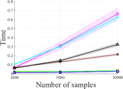
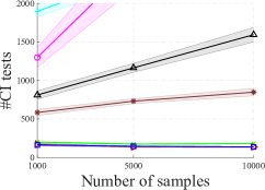
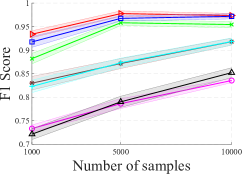
(a) On data; Insurance.

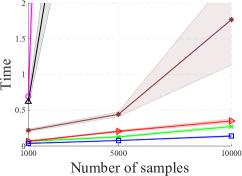
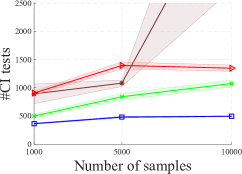
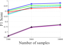
(b) On data; Hepar2.

Figure 5: Performance of various algorithms on two other real-world structures.

Figure 6 shows the runtime of TC algorithm for random Erdos-Renyi graphs when $p=n^{-0.72}$.

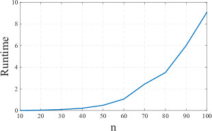
Figure 6: Runtime of TC algorithm for computing Markov boundaries on G(n,p) models where, $p=n^{-0.72}$.

As mentioned in Section 8, alternative values of significance level of CI test do not change our experimental results. Figure 7 illustrates the performance of the BN learning algorithms for different values of the significance level of CI test on Diabetes structure when the number of samples is 5000. As seen in this Figure, the choice of the significance level does not have any considerable effect on our results.

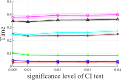
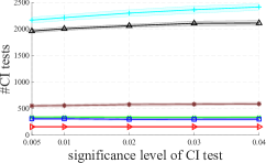
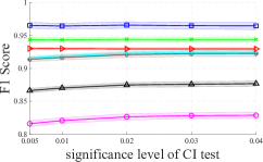
Figure 7: Performance of various algorithms for different values of significance level of CI test on Diabetes structure.

Table 5 demonstrates the experimental results on the real-world structures under two scenarios, namely the oracle setting and the finite sample setting. In the latter scenario (finite sample), the algorithms have access to a dataset with 10,000 samples of each variable. The number of CI tests, Average Size of Conditioning sets (ASC), Accuracy of Learned Separating Sets (ALSS), and runtime of the algorithms are reported after Markov boundary discovery. Structural Hamming Distance (SHD) is calculated as the sum of the number of extra edges and missing edges. Analogous to the the formerly reported results, both RSL algorithms outperform other algorithms in terms of both accuracy and computational complexity.

				Insurance	Hepar2	Diabetes	Andes*	Pigs
				$n=27$	$n=70$	$n=104$	$n=223$	$n=441$
	$RSL_{D}$	Oracle	#CI tests	124	477	250	1,623	1,059
			ASC	1.18	3.38	0.55	2.20	0.55
		finite sample	runtime	0.06	0.18	0.09	0.51	0.63
			F1-score	0.99	0.99	0.96	0.86	0.99
			precision	1	0.99	0.96	0.88	0.99
			recall	0.98	0.97	0.95	0.84	0.99
			SHD	1	5	13	94	11
			ALSS	0.91	0.89	0.87	0.68	0.99
	$RSL_{\omega}$	Oracle	#CI tests	118	1,218	140	2,884	1,059
			ASC	1.42	2.72	1.27	2.40	0.55
		finite sample	runtime	0.04	0.49	0.06	0.94	0.63
			F1-score	0.98	0.94	0.92	0.82	0.99
			precision	0.98	0.89	0.85	0.77	0.99
			recall	0.98	0.99	1	0.88	0.99
			SHD	2	16	25	130	11
			ALSS	0.92	0.86	0.97	0.60	0.99
	MARVEL	Oracle	#CI tests	148	1,663	420	6,072	1,119
			ASC	1.08	2.34	0.71	1.42	0.58
		finite sample	runtime	0.11	0.36	0.18	2.92	0.29
			F1-score	0.99	0.95	0.95	0.77	0.99
			precision	1	0.94	0.93	0.80	0.98
			recall	0.98	0.95	0.96	0.74	0.99
			SHD	1	13	16	150	14
	CS	Oracle	#CI tests	1,079	34,083	901	45,697	20,634
			ASC	2.65	8.25	2.15	5.20	7.94
		finite sample	runtime	0.38	0.78	0.52	10.98	6.99
			F1-score	0.93	0.93	0.93	0.79	0.99
			precision	1	1	0.99	0.97	0.99
			recall	0.86	0.87	0.88	0.66	0.99
			SHD	7	16	19	121	12
	GS	Oracle	#CI tests	1,683	67,408	1,923	56,512	146,888
			ASC	2.88	7.85	2.51	5.37	8.11
		finite sample	runtime	0.75	204.85	0.61	12.36	8.08
			F1-score	0.93	0.74	0.93	0.78	0.99
			precision	1	0.97	1	0.98	0.99
			recall	0.86	0.60	0.88	0.65	0.99
			SHD	7	51	18	122	6
	PC	Oracle	#CI tests	4,912	$>10^{7}$	3,873	40,773	$>10^{13}$
			ASC	3.23	NA	2.20	4.30	NA
		finite sample	runtime	0.35	9.51	0.64	1.26	NA
			F1-score	0.85	0.76	0.87	0.74	NA
			precision	1	1	0.97	0.98	NA
			recall	0.74	0.61	0.80	0.59	NA
			SHD	13	48	34	141	NA
	MMPC	Oracle	#CI tests	4,582	$>10^{6}$	3,543	$>10^{6}$	$>10^{6}$
			ASC	3.35	NA	2.23	NA	NA
		finite sample	runtime	0.56	198.8	0.71	2.70	NA
			F1-score	0.82	0.74	0.84	0.69	NA
			precision	0.90	0.97	0.89	0.89	NA
			recall	0.74	0.60	0.80	0.57	NA
			SHD	17	51	45	169	NA

Table 5: Performance of various algorithms on real-world structures. The structure indicated with star is not diamond-free. NA indicates that the corresponding value is unknown due to a very long runtime.

References

- Améndola et al. (2020) Améndola, C.; Dettling, P.; Drton, M.; Onori, F.; and Wu, J. 2020. Structure Learning for Cyclic Linear Causal Models. In Conference on Uncertainty in Artificial Intelligence, 999–1008. PMLR.
- Andreassen et al. (1991) Andreassen, S.; Hovorka, R.; Benn, J.; Olesen, K. G.; and Carson, E. R. 1991. A model-based approach to insulin adjustment. In AIME 91, 239–248. Springer.
- Bartlett and Cussens (2017) Bartlett, M.; and Cussens, J. 2017. Integer linear programming for the Bayesian network structure learning problem. Artificial Intelligence, 244: 258–271.
- Bodlaender and Möhring (1993) Bodlaender, H. L.; and Möhring, R. H. 1993. The pathwidth and treewidth of cographs. SIAM Journal on Discrete Mathematics, 6(2): 181–188.
- Brandstädt (2004) Brandstädt, A. 2004. (P5, diamond)-free graphs revisited: structure and linear time optimization. Discrete applied mathematics, 138(1-2): 13–27.
- Chen et al. (2016) Chen, E. Y.-J.; Shen, Y.; Choi, A.; and Darwiche, A. 2016. Learning Bayesian networks with ancestral constraints. In Proceedings of the 30th International Conference on Neural Information Processing Systems, 2333–2341. Citeseer.
- Chickering (2002) Chickering, D. M. 2002. Optimal structure identification with greedy search. Journal of machine learning research, 3(Nov): 507–554.
- Chickering, Heckerman, and Meek (2004) Chickering, M.; Heckerman, D.; and Meek, C. 2004. Large-sample learning of Bayesian networks is NP-hard. Journal of Machine Learning Research, 5.
- Claassen, M. Mooij, and Heskes (2013) Claassen, T.; M. Mooij, J.; and Heskes, T. 2013. Learning Sparse Causal Models is not NP-hard. Proceedings of the Twenty-Ninth Conference on Uncertainty in Artificial Intelligence.
- Colombo and Maathuis (2014) Colombo, D.; and Maathuis, M. H. 2014. Order-independent constraint-based causal structure learning. J. Mach. Learn. Res., 15(1): 3741–3782.
- Conati et al. (1997) Conati, C.; Gertner, A. S.; VanLehn, K.; and Druzdzel, M. J. 1997. On-line student modeling for coached problem solving using Bayesian networks. In User Modeling, 231–242. Springer.
- Dabrowski, Dross, and Paulusma (2017) Dabrowski, K. K.; Dross, F.; and Paulusma, D. 2017. Colouring diamond-free graphs. Journal of computer and system sciences, 89: 410–431.
- de Morais and Aussem (2010) de Morais, S. R.; and Aussem, A. 2010. An Efficient and Scalable Algorithm for Local Bayesian Network Structure Discovery. In Machine Learning and Knowledge Discovery in Databases, 164–179.
- Elidan and Gould (2008) Elidan, G.; and Gould, S. 2008. Learning Bounded Treewidth Bayesian Networks. Journal of Machine Learning Research, 9(12).
- Erdős and Rényi (1960) Erdős, P.; and Rényi, A. 1960. On the evolution of random graphs. Publications of the Mathematical Institute of the Hungarian Academy of Sciences, 5: 17–61.
- Fisher (1915) Fisher, R. A. 1915. Frequency distribution of the values of the correlation coefficient in samples from an indefinitely large population. Biometrika, 10(4): 507–521.
- Flores et al. (2011) Flores, M. J.; Nicholson, A. E.; Brunskill, A.; Korb, K. B.; and Mascaro, S. 2011. Incorporating expert knowledge when learning Bayesian network structure: a medical case study. Artificial intelligence in medicine, 53(3): 181–204.
- Friedman et al. (2000) Friedman, N.; Linial, M.; Nachman, I.; and Pe’er, D. 2000. Using Bayesian networks to analyze expression data. Journal of computational biology, 7(3-4): 601–620.
- Ghahramani and Beal (2001) Ghahramani, Z.; and Beal, M. J. 2001. Propagation algorithms for variational Bayesian learning. Advances in neural information processing systems, 507–513.
- Gilbert (1959) Gilbert, E. N. 1959. Random graphs. The Annals of Mathematical Statistics, 30(4): 1141–1144.
- Grüttemeier and Komusiewicz (2020) Grüttemeier, N.; and Komusiewicz, C. 2020. Learning Bayesian Networks Under Sparsity Constraints: A Parameterized Complexity Analysis. arXiv preprint arXiv:2004.14724.
- Huang et al. (2012) Huang, S.; Li, J.; Ye, J.; Fleisher, A.; Chen, K.; Wu, T.; Reiman, E.; Initiative, A. D. N.; et al. 2012. A sparse structure learning algorithm for gaussian bayesian network identification from high-dimensional data. IEEE transactions on pattern analysis and machine intelligence, 35(6): 1328–1342.