Efficient Tensor Robust PCA under Hybrid Model of Tucker and Tensor Train

Abstract

Tensor robust principal component analysis (TRPCA) is a fundamental model in machine learning and computer vision. Recently, tensor train (TT) decomposition has been verified effective to capture the global low-rank correlation for tensor recovery tasks. However, due to the large-scale tensor data in real-world applications, previous TRPCA models often suffer from high computational complexity. In this letter, we propose an efficient TRPCA under hybrid model of Tucker and TT. Specifically, in theory we reveal that TT nuclear norm (TTNN) of the original big tensor can be equivalently converted to that of a much smaller tensor via a Tucker compression format, thereby significantly reducing the computational cost of singular value decomposition (SVD). Numerical experiments on both synthetic and real-world tensor data verify the superiority of the proposed model.

I Introduction

Tensor decomposition is a fundamental tool for multi-way data analysis [1, 2, 3]. In real-world applications, tensor data are often corrupted with sparse outliers or gross noises [4, 5]. For example, face images recorded in practical applications might contaminate gross corruptions due to illumination and occlusion noise. To alleviate this issue, tensor robust principal component analysis [6, 7, 8, 9] (TRPCA) or robust tensor decomposition [10, 11, 12] (RTD) were proposed to estimate the underlying low-rank and sparse components from their sum. In the past decades, it has been shown that the low-rank and sparse components can be exactly recovered by solving the following minimization problem:

$$\min_{\boldsymbol{\mathscr{{X}}},\boldsymbol{\mathscr{{S}}}}\|\boldsymbol{\mathscr{{X}}}\|_{\varoast}+\tau\|\boldsymbol{\mathscr{{S}}}\|_{1},\text{ s.t. }\boldsymbol{\mathscr{{Y}}}=\boldsymbol{\mathscr{{X}}}+\boldsymbol{\mathscr{{S}}},$$ (1)

where $\|\cdot\|_{\varoast}$ and $\|\cdot\|_{1}$ denote tensor nuclear norm and $\ell_{1}$ norm, respectively, and $\tau>0$ is a hyper-parameter balancing the low-rank and sparse components.

The essential element of the TRPCA problem is to capture the high-order low-rank structure. Unlike the matrix case, there is no unified tensor rank definition due to the complex multilinear structure. The most straightforward tensor rank is CANDECOMP/PARAFAC (CP) rank, which is defined on the smallest number of rank-one tensors [1]. Nevertheless, both CP rank and its convex surrogate CP nuclear norm are NP-hard to compute [13, 14]. To alleviate such issue, Zhao et al. [15] proposed a variational Bayesian inference framework for CP rank determination and applied it to the TRPCA problem. Compared with CP rank, Tucker rank is more flexible and interpretable since it explores the low-rank structure in all modes. Tucker rank is defined as a set of ranks of unfolding matrices associated with each mode [16]. Motivated by the convex surrogate of matrix rank, the sum of the nuclear norm (SNN) was adopted as a convex relaxation for Tucker rank [17]. The work [7] proposed an SNN-based TRPCA model. Huang et al. [18] presented the exact recovery guarantee for SNN-based TRPCA. Recently, TT rank-based models have achieved both theoretical and practical performance better than Tucker rank models in the field of tensor recovery applications. Compared with Tucker rank, TT rank was demonstrated to capture global correlation of tensor entries using the concept of von Neumann entropy theory [19]. Gong et al. [20] showed the potential advantages of TT rank by investigating the relationship between Tucker decomposition and TT decomposition. Similar to SNN, Bengua et al. [19] proposed TT nuclear norm (TTNN) using the sum of nuclear norm of TT unfolding matrix along with each mode. Yang et al. [21] proposed a TRPCA model based on TTNN and applied it to tensor denoising tasks.

It is significantly important to have efficient optimization algorithms for TRPCA problem. This is especially challenging for large-scale and high-order tensor data. In this letter, we propose an efficient TT rank-based TRPCA model which equivalently converts the TTNN minimization problem of the original tensor to that of a much smaller tensor. Thus, the computational complexity of TTNN minimization problem can be significantly reduced. To summarize, we make the following contributions:

• We demonstrate that the minimization of TTNN on the original big tensor can be equivalently converted to a much smaller tensor under a Tucker compression format.

• We propose an efficient TRPCA model and develop an effective alternating direction method of multipliers (ADMM) based optimization algorithm.

• We finally show that the proposed model achieves more promising recovery performance and less running time than the state-of-the-art models on both synthetic and real-world tensor data.

II Notation and Preliminary

II-A Notations

We adopt the notations used in [1]. The set $\{1,2,\cdots,K\}$ is denoted as $[K]$. A scalar is given by a standard lowercases or uppercases letter $x,X\in\mathbb{R}$. A matrix is given by a boldface capital letter $\boldsymbol{\mathbf{X}}\in\mathbb{R}^{d_{1}\times d_{2}}$. A tensor is given by calligraphic letter $\boldsymbol{\mathscr{{X}}}\in\mathbb{R}^{d_{1}\times d_{2}\times\cdots d_{K}}$. The $(i_{1},i_{2},\cdots,i_{K})$ entry of tensor $\boldsymbol{\mathscr{{X}}}$ is given by $X(i_{1},i_{2},\cdots,i_{K})$. The standard mode-$k$ unfolding [1] of tensor $\boldsymbol{\mathscr{{X}}}\in\mathbb{R}^{d_{1}\times d_{2}\times\cdots\times d_{K}}$ is given by $\boldsymbol{\mathbf{X}}_{(k)}\in\mathbb{R}^{d_{k}\times d_{1}\cdots d_{k-1}d_{k+1}\cdots d_{K}}$, and the corresponding matrix-tensor folding operation is given by ${\leavevmode\lstinline{{\lst@@@set@language\lst@@@set@numbers\lst@@@set@frame\lst@@@set@rulecolor\lst@@@set@language\footnotesize\small{\@listingGroup{}{ld}}}}}_{k}(\boldsymbol{\mathbf{X}}_{(k)})$. Another mode-$k$ unfolding for TT decomposition [22] is denoted as $\boldsymbol{\mathbf{X}}_{[k]}\in\mathbb{R}^{d_{1}\cdots d_{k-1}\times d_{k}\cdots d_{K}}$, and the corresponding matrix-tensor folding operation is denoted as ${\leavevmode\lstinline{{\lst@@@set@language\lst@@@set@numbers\lst@@@set@frame\lst@@@set@rulecolor\lst@@@set@language\footnotesize\small{\@listingGroup{}{d}}}}}_{k}(\boldsymbol{\mathbf{X}}_{[k]})$.

II-B Tensor Train Decomposition

Definition 1 (TT decomposition [22]).

The tensor train (TT) decomposition represents a $K$th-order tensor $\boldsymbol{\mathscr{{Y}}}\in\mathbb{R}^{d_{1}\times\cdots\times d_{K}}$ by the sequence multilinear product over a set of third-order core tensors, i.e., ${\boldsymbol{\mathscr{{Y}}}=\emph{\leavevmode\lstinline{{\lst@@@set@language\lst@@@set@numbers\lst@@@set@frame\lst@@@set@rulecolor\lst@@@set@language\footnotesize\small{\@listingGroup{ltx_lst_identifier}{TT}}}}}}(\boldsymbol{\mathscr{{G}}}^{(1)},\cdots,\boldsymbol{\mathscr{{G}}}^{(K)})$, where $\boldsymbol{\mathscr{{G}}}^{(k)}\in\mathbb{R}^{r_{k-1}\times d_{k}\times r_{k}}$, $k\in[K]$, and $r_{K}=r_{0}=1$. Element-wisely, it can be represented as

$${Y}({i_{1},i_{2},\cdots,i_{K}})=\sum_{\upsilon_{0},\cdots,\upsilon_{K}}^{r_{0},\cdots,r_{K}}\prod_{k=1}^{K}{G}^{(k)}(\upsilon_{k-1},i_{k},\upsilon_{k}).$$ (2)

The size of cores, $r_{k},k=1,\cdots,K-1$, denoted by a vector $[r_{1},\cdots,r_{K-1}]$, is called TT rank.

Definition 2 (TT nuclear norm [19]).

The tensor train nuclear norm (TTNN) is defined by the weighted sum of nuclear norm along each unfolding matrix:

$$\|\boldsymbol{\mathscr{{Y}}}\|_{\emph{ttnn}}:=\sum_{k=1}^{K-1}\alpha_{k}\|\boldsymbol{\mathbf{Y}}_{[k]}\|_{*},$$ (3)

where $\|\cdot\|_{*}$ is the matrix nuclear norm, $\alpha_{k}>0$ denotes the weight of mode-$k$ unfolding.

III Efficient TRPCA under Hybrid Model of Tucker and TT

III-A Fast TTNN Minimization under a Tucker Compression

In the following theorem, we show that TT decomposition can be equivalently given in a Tucker compression format.

Theorem 1.

Let $\boldsymbol{\mathscr{{X}}}\in\mathbb{R}^{d_{1}\times d_{2}\times\cdots\times d_{K}}$ be a $K$th-order tensor with TT rank $[r_{1},\cdots r_{K-1}]$, it can be formulated as the following Tucker decomposition format:

$$\boldsymbol{\mathscr{{X}}}=\tilde{\boldsymbol{\mathscr{{X}}}}\times_{1}\boldsymbol{\mathbf{U}}_{1}\times_{2}\cdots\times_{K}\boldsymbol{\mathbf{U}}_{K},\boldsymbol{\mathbf{U}}_{k}\in St(d_{k},R_{k}),$$ (4)

where ${\tilde{\boldsymbol{\mathscr{{X}}}}=\emph{\leavevmode\lstinline{{\lst@@@set@language\lst@@@set@numbers\lst@@@set@frame\lst@@@set@rulecolor\lst@@@set@language\footnotesize\small{\@listingGroup{ltx_lst_identifier}{TT}}}}}}(\tilde{\boldsymbol{\mathscr{{G}}}}^{(1)},\tilde{\boldsymbol{\mathscr{{G}}}}^{(2)},\cdots,\tilde{\boldsymbol{\mathscr{{G}}}}^{(K)})$ denotes the core tensor, $\tilde{\boldsymbol{\mathscr{{G}}}}^{(k)}\in\mathbb{R}^{r_{k}\times R_{k}\times r_{k+1}}$, and $St(d_{k},R_{k}):=\{\boldsymbol{\mathbf{U}}\in\mathbb{R}^{d_{k}\times R_{k}},\boldsymbol{\mathbf{U}}^{\top}\boldsymbol{\mathbf{U}}=\boldsymbol{\mathbf{I}}_{R_{k}}\}$ is the Stiefel manifold.

Proof.

The proof can be completed by discussing in the following two cases.

Case 1: If $d_{k}>r_{k}r_{k+1}$, we let $\boldsymbol{\mathbf{U}}_{k}$ be the left singular matrix of mode-2 unfolding of $\boldsymbol{\mathscr{{G}}}^{(k)}$, i.e., ${[\boldsymbol{\mathbf{U}}_{k},\bm{\Sigma}_{k},\boldsymbol{\mathbf{V}}_{k}^{\top}]=\leavevmode\lstinline{{\lst@@@set@language\lst@@@set@numbers\lst@@@set@frame\lst@@@set@rulecolor\lst@@@set@language\footnotesize\small{\@listingGroup{}{}}}}}(\boldsymbol{\mathbf{G}}^{(k)}_{(2)})$, and we let ${\tilde{\boldsymbol{\mathscr{{G}}}}^{(k)}=\leavevmode\lstinline{{\lst@@@set@language\lst@@@set@numbers\lst@@@set@frame\lst@@@set@rulecolor\lst@@@set@language\footnotesize\small{\@listingGroup{}{ld}}}}}_{2}(\bm{\Sigma}_{k}\boldsymbol{\mathbf{V}}_{k}^{\top})$.

Case 2: If $d_{k}\leq r_{k}r_{k+1}$, we let $\boldsymbol{\mathbf{U}}_{k}$ be the identity matrix, i.e., $\boldsymbol{\mathbf{U}}_{k}=\boldsymbol{\mathbf{I}}_{d_{k}}$, and $\tilde{\boldsymbol{\mathscr{{G}}}}^{(k)}=\boldsymbol{\mathscr{{G}}}^{(k)}$.

Combing these two cases, the core tensor of TT decomposition can be given by $\boldsymbol{\mathscr{{G}}}^{(k)}=\tilde{\boldsymbol{\mathscr{{G}}}}^{(k)}\times_{2}\boldsymbol{\mathbf{U}}_{k},k\in[K]$. Element-wisely, we can present TT decomposition of $\boldsymbol{\mathscr{{X}}}$ as

$${{\begin{split}&X({i_{1},\cdots,i_{K}})\\ =&\boldsymbol{\mathbf{G}}^{(1)}(:,i_{1},:)\boldsymbol{\mathbf{G}}^{(2)}(:,i_{2},:)\cdots\boldsymbol{\mathbf{G}}^{(K)}(:,i_{K},:)\\ =&\sum_{j_{1}=1}^{R_{1}}\cdots\sum_{j_{K}=1}^{R_{K}}\tilde{\boldsymbol{\mathbf{G}}}^{(1)}(:,j_{1},:){U}_{1}(j_{1},i_{1})\\ &\tilde{\boldsymbol{\mathbf{G}}}^{(2)}(:,j_{2},:){U}_{2}(j_{2},i_{2})\cdots\tilde{\boldsymbol{\mathbf{G}}}^{(K)}(:,j_{K},:){U}_{K}(j_{K},i_{K})\\ =&\sum_{j_{1}=1}^{R_{1}}\cdots\sum_{j_{K}=1}^{R_{K}}\tilde{\boldsymbol{\mathbf{G}}}^{(1)}(:,j_{1},:)\tilde{\boldsymbol{\mathbf{G}}}^{(2)}(:,j_{2},:)\cdots\\ &\tilde{\boldsymbol{\mathbf{G}}}^{(K)}(:,j_{K},:){U}_{1}(j_{1},i_{1}){U}_{2}(j_{2},i_{2})\cdots{U}_{K}(j_{K},i_{K})\\ =&\sum_{j_{1}=1}^{R_{1}}\cdots\sum_{j_{K}=1}^{R_{K}}\leavevmode\lstinline{{\lst@@@set@language\lst@@@set@numbers\lst@@@set@frame\lst@@@set@rulecolor\lst@@@set@language\footnotesize\small{\@listingGroup{ltx_lst_identifier}{TT}}}}}(\tilde{\boldsymbol{\mathscr{{G}}}}^{(1)},\cdots,\tilde{\boldsymbol{\mathscr{{G}}}}^{(K)})(i_{1},\cdots,i_{K})\\ &{U}_{1}(j_{1},i_{1})\cdots{U}_{K}(j_{K},i_{K})\\ =&\leavevmode\lstinline{{\lst@@@set@language\lst@@@set@numbers\lst@@@set@frame\lst@@@set@rulecolor\lst@@@set@language\footnotesize\small{\@listingGroup{ltx_lst_identifier}{TT}}}}}(\tilde{\boldsymbol{\mathscr{{G}}}}^{(1)},\cdots,\tilde{\boldsymbol{\mathscr{{G}}}}^{(K)})\times_{1}\boldsymbol{\mathbf{U}}_{1}(:,i_{1})\cdots\times_{K}\boldsymbol{\mathbf{U}}_{K}(:,i_{K}).\\ \end{split}$$ (5)

Thus, we have $\boldsymbol{\mathscr{{X}}}=\tilde{\boldsymbol{\mathscr{{X}}}}\times_{1}\boldsymbol{\mathbf{U}}_{1}\cdots\times_{K}\boldsymbol{\mathbf{U}}_{K}$, where ${\tilde{\boldsymbol{\mathscr{{X}}}}=\leavevmode\lstinline{{\lst@@@set@language\lst@@@set@numbers\lst@@@set@frame\lst@@@set@rulecolor\lst@@@set@language\footnotesize\small{\@listingGroup{ltx_lst_identifier}{TT}}}}}(\tilde{\boldsymbol{\mathscr{{G}}}}^{(1)},\tilde{\boldsymbol{\mathscr{{G}}}}^{(2)},\cdots,\tilde{\boldsymbol{\mathscr{{G}}}}^{(K)})$ and $\boldsymbol{\mathbf{U}}_{k}\in St(d_{k},R_{k}),k\in[K]$.

Proof of Theorem 1 is completed. ∎

In the next theorem, we demonstrate that under a Tucker compression format, TTNN of the original tensor can be equivalently converted to that of a much smaller tensor.

Theorem 2.

Let $\boldsymbol{\mathscr{{X}}}\in\mathbb{R}^{d_{1}\times\cdots\times d_{K}}$ be a $K$th-order tensor with TT rank $[r_{1},\cdots r_{K-1}]$, the TTNN of $\boldsymbol{\mathscr{{X}}}$ can be given by

$$\|\boldsymbol{\mathscr{{X}}}\|_{\emph{ttnn}}=\|\tilde{\boldsymbol{\mathscr{{X}}}}\|_{\emph{ttnn}},$$ (6)

where $\boldsymbol{\mathscr{{X}}}=\tilde{\boldsymbol{\mathscr{{X}}}}\times_{1}\boldsymbol{\mathbf{U}}_{1}\cdots\times_{K}\boldsymbol{\mathbf{U}}_{K},\boldsymbol{\mathbf{U}}_{k}\in St(d_{k},R_{k}),k\in[K]$.

Proof.

According to Lemma 3 in [23], we have

$$\boldsymbol{\mathbf{X}}_{[k]}=(\boldsymbol{\mathbf{U}}_{k}\otimes\cdots\otimes\boldsymbol{\mathbf{U}}_{1})\tilde{\boldsymbol{\mathbf{X}}}_{[k]}(\boldsymbol{\mathbf{U}}_{K}\otimes\cdots\otimes\boldsymbol{\mathbf{U}}_{k+1})^{\top}.$$ (7)

Note that the Kronecker product of multiple orthogonal matrices is still orthogonal matrix, that is,

$$\begin{split}&(\boldsymbol{\mathbf{U}}_{k}\otimes\cdots\otimes\boldsymbol{\mathbf{U}}_{1})^{\top}(\boldsymbol{\mathbf{U}}_{k}\otimes\cdots\otimes\boldsymbol{\mathbf{U}}_{1})\\ &=(\boldsymbol{\mathbf{U}}_{k}^{\top}\boldsymbol{\mathbf{U}}_{k}\otimes\cdots\otimes\boldsymbol{\mathbf{U}}_{1}^{\top}\boldsymbol{\mathbf{U}}_{1})=\boldsymbol{\mathbf{I}}_{M},\end{split}$$ (8)

where $M=\prod_{j=1}^{k}{R_{j}}$. Combining Eq. (8) and Eq. (7), we have

$$\|\boldsymbol{\mathbf{X}}_{[k]}\|_{*}=\|\tilde{\boldsymbol{\mathbf{X}}}_{[k]}\|_{*},k\in[K-1].$$ (9)

Proof of Theorem 2 is completed. ∎

Algorithm 1 Optimization Algorithm for FTTNN-based TRPCA Model

0:  $\boldsymbol{\mathscr{{Y}}},\tau.$

0:  $\mu=10^{-2},\mu_{\text{max}}=10^{10},\rho=1.1,tol=10^{-8}$, $\boldsymbol{\mathscr{{G}}}^{(k)}$ using $\mathcal{N}(0,1)$ distribution.

1:  while not converge do

2:     Update ${\boldsymbol{\mathscr{{M}}}^{k,t+1}=\leavevmode\lstinline{{\lst@@@set@language\lst@@@set@numbers\lst@@@set@frame\lst@@@set@rulecolor\lst@@@set@language\footnotesize\small{\@listingGroup{}{d}}}}}_{k}\Big{(}\mathcal{D}_{\alpha_{k}/\mu}(\tilde{\boldsymbol{\mathbf{X}}}_{[k]}^{t}-\frac{1}{\mu}\boldsymbol{\mathbf{Q}}_{[k]}^{k,t})\Big{)}$, where $\mathcal{D}_{\alpha_{k}/\mu}(\cdot)$ denotes the SVT operator [24].

3:     Update $\boldsymbol{\mathscr{{X}}}^{t+1}=\boldsymbol{\mathscr{{Y}}}^{t}-\boldsymbol{\mathscr{{S}}}^{t}+\tilde{\boldsymbol{\mathscr{{X}}}}^{t}\times_{1}\boldsymbol{\mathbf{U}}_{1}^{t}\cdots\times_{K}\boldsymbol{\mathbf{U}}_{K}^{t}+\frac{1}{\mu}(\boldsymbol{\mathscr{{E}}}^{t}-\boldsymbol{\mathscr{{P}}}^{t}).$

4:     Update $\boldsymbol{\mathscr{{S}}}^{t+1}=\mathcal{S}_{\tau}(\boldsymbol{\mathscr{{Y}}}^{t}-\boldsymbol{\mathscr{{X}}}^{t+1}+\frac{1}{\mu}\boldsymbol{\mathscr{{E}}}^{t})$, where $\mathcal{S}_{\tau}$ denotes the soft-shrinkage operator [25].

5:     Update $\tilde{\boldsymbol{\mathscr{{X}}}}^{t+1}=\frac{1}{K\mu}\Big{(}(\mu\boldsymbol{\mathscr{{X}}}^{t+1}+\boldsymbol{\mathscr{{P}}}^{t})\times_{1}\boldsymbol{\mathbf{U}}_{1}^{t,\top}\cdots\times_{K}\boldsymbol{\mathbf{U}}_{K}^{t,\top}+\sum_{k=1}^{K}\mu\boldsymbol{\mathscr{{M}}}^{k,t}+\boldsymbol{\mathscr{{Q}}}^{k,t}\Big{)}$.

6:     Update $\boldsymbol{\mathbf{U}}_{k}^{t+1}=\boldsymbol{\mathbf{A}}_{k}\boldsymbol{\mathbf{B}}_{k}$, where $(\frac{1}{\mu}\boldsymbol{\mathbf{P}}_{(k)}^{t}+\boldsymbol{\mathbf{X}}_{(k)}^{t+1})\boldsymbol{\mathbf{V}}_{(k)}=\boldsymbol{\mathbf{A}}_{k}\boldsymbol{\mathbf{D}}_{k}\boldsymbol{\mathbf{B}}_{k}$ is the SVD of $(\frac{1}{\mu}\boldsymbol{\mathbf{P}}_{(k)}+\boldsymbol{\mathbf{X}}_{(k)})\boldsymbol{\mathbf{V}}_{(k)}$, and $\boldsymbol{\mathscr{{V}}}=\boldsymbol{\mathscr{{X}}}^{t+1}\times_{1}\boldsymbol{\mathbf{U}}_{1}^{t+1,\top}\cdots\times_{k-1}\boldsymbol{\mathbf{U}}_{k-1}^{t+1,\top}\times_{k+1}\boldsymbol{\mathbf{U}}_{k+1}^{t,\top}\cdots\boldsymbol{\mathbf{U}}_{K}^{t,\top}$.

7:     Update $\boldsymbol{\mathscr{{Q}}}^{k,t+1}=\boldsymbol{\mathscr{{Q}}}^{k,t}+\mu(\boldsymbol{\mathscr{{M}}}^{k,t+1}-\tilde{\boldsymbol{\mathscr{{X}}}}^{t+1}),k\in[K-1]$.

8:     Update $\boldsymbol{\mathscr{{P}}}^{t+1}=\boldsymbol{\mathscr{{P}}}^{t}+\mu(\boldsymbol{\mathscr{{X}}}^{t+1}-\tilde{\boldsymbol{\mathscr{{X}}}}^{t+1}\times_{1}\boldsymbol{\mathbf{U}}_{1}^{t+1}\times_{2}\cdots\times_{K}\boldsymbol{\mathbf{U}}_{K}^{t+1})$.

9:     Update $\mu=\max(\rho\mu,\mu_{\text{max}})$.

10:     Check the convergence condition:

11:     $\max\big{(}\frac{\|\boldsymbol{\mathscr{{S}}}_{t+1}-\boldsymbol{\mathscr{{S}}}_{t}\|_{F}}{\|\boldsymbol{\mathscr{{S}}}_{t}\|_{F}},\frac{\|\boldsymbol{\mathscr{{X}}}_{t+1}-\boldsymbol{\mathscr{{X}}}_{t}\|_{F}}{\|\boldsymbol{\mathscr{{X}}}_{t}\|_{F}}\big{)}\leq tol$.

12:     $t\leftarrow t+1$.

13:  end while

III-B Efficient TRPCA under Hybrid Model of Tucker and TT

TRPCA aims to recover the low-rank and sparse components from their sum. The low-rank TT-based TRPCA model can be formulated as

$$\min_{\boldsymbol{\mathscr{{X}}},\boldsymbol{\mathscr{{S}}}}\|\boldsymbol{\mathscr{{X}}}\|_{\text{ttnn}}+\tau\|\boldsymbol{\mathscr{{S}}}\|_{1}\\ \text{ s.t. }\boldsymbol{\mathscr{{Y}}}=\boldsymbol{\mathscr{{X}}}+\boldsymbol{\mathscr{{S}}},$$ (10)

where $\tau>0$ denotes the hyper-parameter. Combining Theorem 1 and Theorem 2, problem (10) can be equivalently given in a fast TTNN (FTTNN) minimization format:

$$\begin{split}&\min_{\boldsymbol{\mathscr{{X}}},\tilde{\boldsymbol{\mathscr{{X}}}},\boldsymbol{\mathscr{{S}}},\{\boldsymbol{\mathbf{U}}_{k}\}_{k=1}^{K}}\|\tilde{\boldsymbol{\mathscr{{X}}}}\|_{\text{ttnn}}+\tau\|\boldsymbol{\mathscr{{S}}}\|_{1}\\ \text{s.t. }&\boldsymbol{\mathscr{{X}}}=\tilde{\boldsymbol{\mathscr{{X}}}}\times_{1}\boldsymbol{\mathbf{U}}_{1}\times_{2}\cdots\times_{K}\boldsymbol{\mathbf{U}}_{K},\\ &\boldsymbol{\mathscr{{Y}}}=\boldsymbol{\mathscr{{X}}}+\boldsymbol{\mathscr{{S}}},\boldsymbol{\mathbf{U}}_{k}\in St(I_{k},R_{k}).\end{split}$$ (11)

By incorporating auxiliary variables $\{\boldsymbol{\mathscr{{M}}}^{k}\}_{k=1}^{K}$, the augmented Lagrangian function of problem (11) is given by

$$\begin{split}&L_{\mu}(\{\boldsymbol{\mathscr{{M}}}^{k}\}_{k=1}^{K-1},\tilde{\boldsymbol{\mathscr{{X}}}},\boldsymbol{\mathscr{{S}}},\{\boldsymbol{\mathbf{U}}_{k}\}_{k=1}^{K},\{\boldsymbol{\mathscr{{Q}}}^{k}\}_{k=1}^{K-1},\boldsymbol{\mathscr{{E}}},\boldsymbol{\mathscr{{P}}})\\ =&\sum_{k=1}^{K-1}\alpha_{k}\|\boldsymbol{\mathbf{M}}_{[k]}^{k}\|_{*}+\tau\|\boldsymbol{\mathscr{{S}}}\|_{1}\\ &+\sum_{k=1}^{K-1}\langle\boldsymbol{\mathscr{{Q}}}^{k},\boldsymbol{\mathscr{{M}}}^{k}-\tilde{\boldsymbol{\mathscr{{X}}}}\rangle+\frac{\mu}{2}\|\boldsymbol{\mathscr{{M}}}^{k}-\tilde{\boldsymbol{\mathscr{{X}}}}\|_{F}^{2}\\ &+\langle\boldsymbol{\mathscr{{Y}}}-\boldsymbol{\mathscr{{X}}}-\boldsymbol{\mathscr{{S}}},\boldsymbol{\mathscr{{E}}}\rangle+\frac{\mu}{2}\|\boldsymbol{\mathscr{{Y}}}-\boldsymbol{\mathscr{{X}}}-\boldsymbol{\mathscr{{S}}}\|_{F}^{2}\\ &+\langle\boldsymbol{\mathscr{{P}}},\boldsymbol{\mathscr{{X}}}-\tilde{\boldsymbol{\mathscr{{X}}}}\times_{1}\boldsymbol{\mathbf{U}}_{1}\times_{2}\cdots\times_{K}\boldsymbol{\mathbf{U}}_{K}\rangle\\ &+\frac{\mu}{2}\|\boldsymbol{\mathscr{{X}}}-\tilde{\boldsymbol{\mathscr{{X}}}}\times_{1}\boldsymbol{\mathbf{U}}_{1}\times_{2}\cdots\times_{K}\boldsymbol{\mathbf{U}}_{K}\|_{F}^{2}\\ \text{s.t. }&\boldsymbol{\mathbf{U}}_{k}\in St(I_{k},R_{k}),k\in[K],\end{split}$$ (12)

where $\mu>0$ denotes penalty parameter, $\{\boldsymbol{\mathscr{{Q}}}^{k}\}_{k=1}^{K},\boldsymbol{\mathscr{{E}}}$ and $\boldsymbol{\mathscr{{P}}}$ are Lagrange multipliers. All variables of Eq. (12) can be solved separately based on ADMM method [26]. The update details are summarized in Algorithm 1.

Compared with the time complexity $\mathcal{O}(d^{3K/2})$ in TTNN of the original big tensor, the proposed FTTNN-based TRPCA model only requires time complexity $\mathcal{O}(KR^{2}d^{K-1}+KR^{3K/2}+KRd^{K})$, which will greatly accelerate the optimization algorithm if the given rank $R$ is significantly low.

TABLE I: Recovery Results of the Proposed FTTNN and TTNN on Synthetic Tensor Data

d	TT rank	NR	Alg	RSE-$\boldsymbol{\mathscr{{X}}}$	RSE-$\boldsymbol{\mathscr{{S}}}$	Time
30	3	5%	TTNN	1.52e-8	1.36e-10	18.05
			FTTNN (ours)	1.83e-9	3.63e-11	7.29
		10%	TTNN	1.54e-8	1.30e-10	20.34
			FTTNN (ours)	1.41e-9	2.31e-11	7.81
	4	5%	TTNN	1.52e-8	2.09e-10	17.64
			FTTNN (ours)	1.52e-9	4.72e-11	8.29
		10%	TTNN	1.49e-8	2.00e-10	19.03
			FTTNN (ours)	1.06e-9	2.69e-11	8.47
40	4	5%	TTNN	1.46e-8	1.07e-10	129.69
			FTTNN (ours)	1.89e-9	3.40e-11	23.27
		10%	TTNN	1.31e-8	9.64e-11	122.99
			FTTNN (ours)	1.26e-9	1.77e-11	24.46
	5	5%	TTNN	1.31e-8	1.40e-10	112.36
			FTTNN (ours)	1.45e-9	3.60e-11	28.58
		10%	TTNN	1.32e-8	1.34e-10	117.01
			FTTNN (ours)	5.46e-7	1.25e-8	27.72

IV Numerical Experiments

In this section, we present the numerical experiment results on synthetic tensor data as well as color image and video data, of the proposed and state-of-the-art model, namely BRTF [15], SNN [7], tSVD [6] and TTNN [21]. All experiments are tested with respect to different sparse noise ratios (NR), which is given by $\text{NR}=N/\prod_{k=1}^{K}d_{k}\times 100\%$, where $N$ denotes the number of sparse component entries. The relative standard error (RSE) is adopted as a performance metric, and is given by $\text{RSE}=\|\boldsymbol{\mathscr{{X}}}^{*}-\boldsymbol{\mathscr{{X}}}_{0}\|_{F}/\|\boldsymbol{\mathscr{{X}}}_{0}\|_{F}$, where $\boldsymbol{\mathscr{{X}}}^{*}$ and $\boldsymbol{\mathscr{{X}}}_{0}$ are the estimated and true tensor, respectively. Matlab implementation of the proposed method is publicly available .

IV-A Synthetic Data

We generate a low-rank tensor $\boldsymbol{\mathscr{{X}}}_{0}\in\mathbb{R}^{d\times d\times d\times d}$ by TT contraction [22] with TT rank $[r,r,r]$. The entries of each core tensor are generated by i.i.d. standard Gaussian distribution, i.e., $g_{v_{k},i_{k},v_{k+1}}^{(k)}\sim\mathcal{N}(0,1),k\in[K]$. The support of sparse noise $\boldsymbol{\mathscr{{S}}}_{0}$ is uniformly sampled at random. For $(i_{1},i_{2},i_{3},i_{4})\in\text{supp}(\boldsymbol{\mathscr{{S}}}_{0})$, we let $\boldsymbol{\mathscr{{S}}}_{0}(i_{1},i_{2},i_{3},i_{4})=\boldsymbol{\mathscr{{B}}}(i_{1},i_{2},i_{3},i_{4})$, where $\boldsymbol{\mathscr{{B}}}$ is generated by the independent Bernoulli distribution. The observed tensor is formed by $\boldsymbol{\mathscr{{Y}}}=\boldsymbol{\mathscr{{X}}}_{0}+\boldsymbol{\mathscr{{S}}}_{0}$. The parameter $\tau=1/(K-1)\sum_{k=1}^{K-1}1/\sqrt{\max(d_{1,k},d_{2,k})}$. For the weight $\alpha_{k},k\in[K-1],$ we adopt the same strategy used in [19].

IV-A1 Effectiveness of the Proposed FTTNN-based TRPCA

To verify the effectiveness of the proposed FTTNN-based TRPCA, we conduct experiments on multiple conditions. We let $d\in\{30,40\}$, and $r\in\{3,4,5\}$. The sparse noise ratio is selected in a candidate set: $\text{NR}\in\{5\%,10\%\}$. The given rank is set to ${R_{1}=R_{4}=\leavevmode\lstinline{{\lst@@@set@language\lst@@@set@numbers\lst@@@set@frame\lst@@@set@rulecolor\lst@@@set@language\footnotesize\small{\@listingGroup{}{nd}}}}}(1.2r)$ and ${R_{2}=R_{3}=\leavevmode\lstinline{{\lst@@@set@language\lst@@@set@numbers\lst@@@set@frame\lst@@@set@rulecolor\lst@@@set@language\footnotesize\small{\@listingGroup{}{nd}}}}}(1.2r^{2})$. For each fixed setting, we repeat the experiment 10 times and report their average. Table I shows the results of FTTNN and TTNN on synthetic tensor data. As can be seen, FTTNN provides lower RSE on both low-rank $\boldsymbol{\mathscr{{X}}}$ and sparse $\boldsymbol{\mathscr{{S}}}$ components compared with TTNN in most cases. Moreover, FTTNN is at least 2 times faster than TTNN when $d=30$ and at least 4 times faster than TTNN when $d=40$.

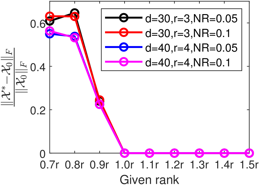
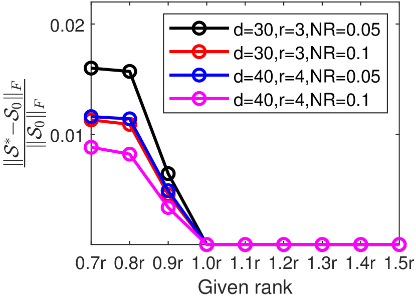
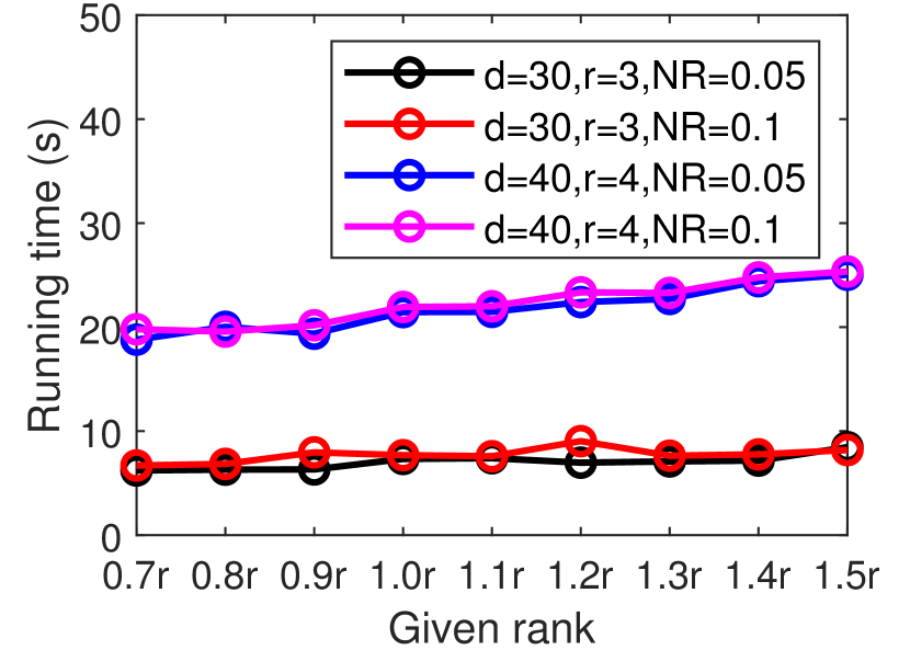
Figure 1: Plots of RSE of recovered $\boldsymbol{\mathscr{{X}}}^{*}$, $\boldsymbol{\mathscr{{S}}}^{*}$ and running time versus varying initialization of rank. (a) RSE-$\boldsymbol{\mathscr{{X}}}$ versus different ranks; (b) RSE-$\boldsymbol{\mathscr{{S}}}$ versus different ranks; (c) Running time versus different ranks.

IV-A2 Robustness of the Given Rank

In this part, we investigate robustness of the given rank for FTTNN. Similar with the above simulation, we set $d\in\{30,40\}$, $r\in\{3,4\}$ and let the sparse noise ratio $\text{NR}\in\{5\%,10\%\}$. The given rank of the proposed model is set to ${R_{1}=R_{4}=\leavevmode\lstinline{{\lst@@@set@language\lst@@@set@numbers\lst@@@set@frame\lst@@@set@rulecolor\lst@@@set@language\footnotesize\small{\@listingGroup{}{nd}}}}}(qr)$ and ${R_{2}=R_{3}=\leavevmode\lstinline{{\lst@@@set@language\lst@@@set@numbers\lst@@@set@frame\lst@@@set@rulecolor\lst@@@set@language\footnotesize\small{\@listingGroup{}{nd}}}}}(qr^{2})$ with $q\in\{0.7,0.8,\cdots,1.5\}$. In Fig. 1, we plot its average RSE and running time versus different given ranks. It can be observed that the proposed FTTNN achieves stable recovery performance versus different given ranks if $q\geq 1$, which verifies the correctness of Theorem 2. Additionally, running time of the proposed FTTNN grows slowly as the given rank increases.

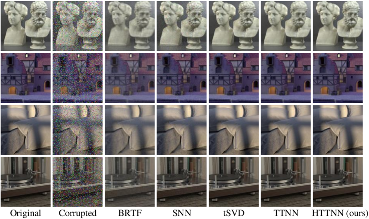
Figure 2: Visual performance of the proposed FTTNN compared with related BRTF, SNN, tSVD and TTNN (best seen in larger resolution on monitor).

TABLE II: Average Recovery Results of Compared Models on Four Benchmark Images

Models	greek	medieval2	pillows	vinyl	Avg. time
Noisy	0.2753	0.5175	0.3364	0.5854	-
BRTF	0.0934	0.1666	0.0941	0.1965	112.75
SNN	0.0733	0.0859	0.0535	0.0852	930.04
tSVD	0.0516	0.0497	0.0383	0.0524	71.67
TTNN	0.0447	0.0403	0.0310	0.0333	104.68
FTTNN (ours)	0.0354	0.0348	0.0207	0.0286	53.13

IV-B Robust Recovery of Noisy Light Field Images

In this part, we conduct robust noisy light field image recovery experiment on four light field benchmark images, namely, “greek”,“medieval2”,“pillows” and “vinyl”. The dimensions of each image is down sampled to $128\times 128\times 3\times 81$. The given rank of the proposed model is set to $[80,80,3,10]$ and the weight $\alpha$ is set to $[0.1,0.8,0.1]$. For each image, we randomly select $20\%$ entries with their values being randomly distributed in $[0,255]$. Fig. 2 depicts the $50$th recovered image, i.e., $\boldsymbol{\mathscr{{Y}}}(:,:,:,50)$. From Fig. 2, we can observe that the results obtained by the proposed FTTNN are superior to the compared models, especially for the recovery of local details. Table II shows the recovered RSE and average running time on four benchmark images. Compared with the state-of-the-art models, the proposed FTTNN achieves both minimum RSE and average running time in all light field images, which indicates its efficiency.

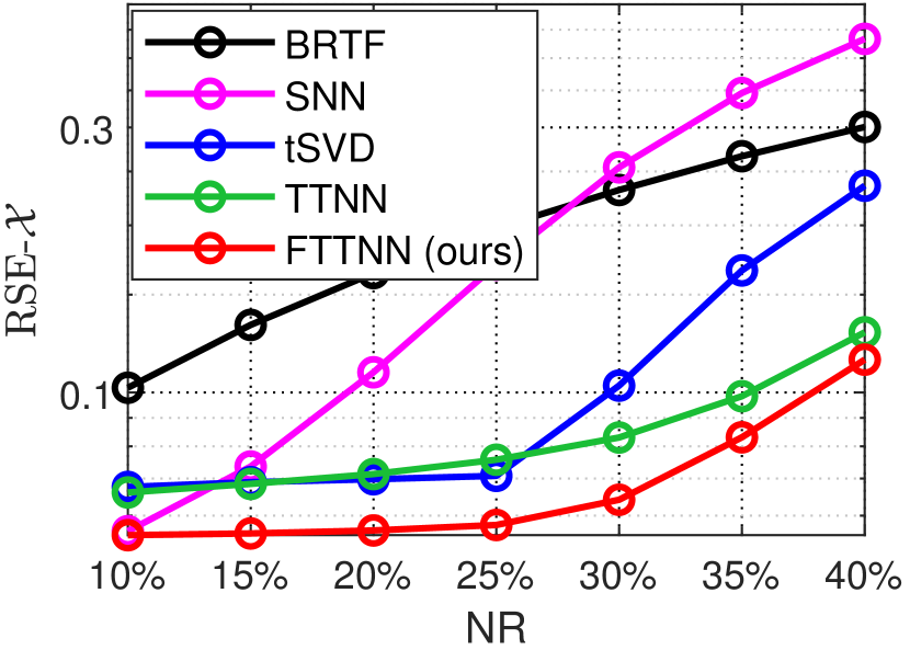
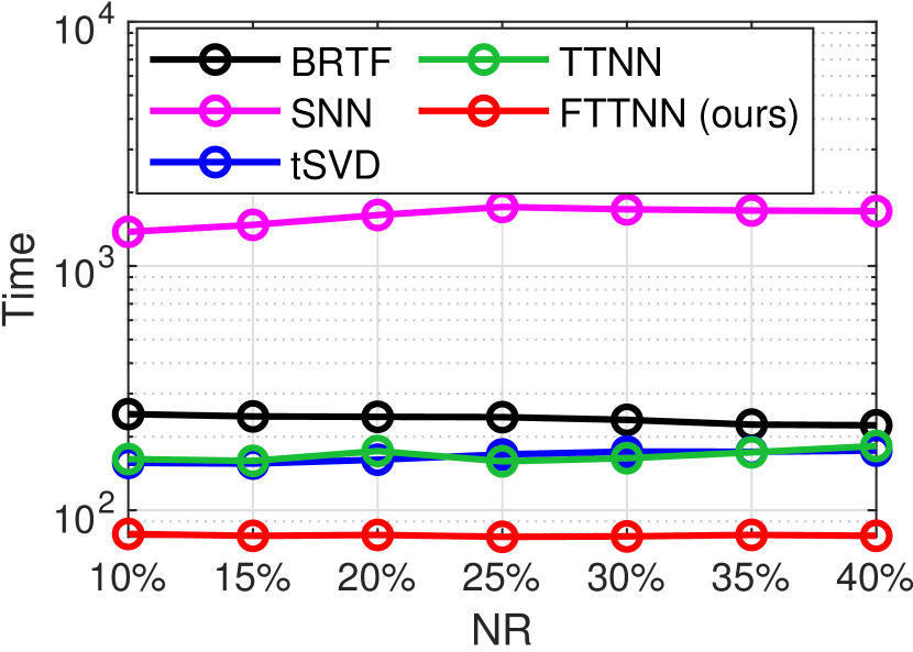
Figure 3: Plots of average RSE and running time of compared models under different NR. (a) RSE versus NR; (b) running time versus NR.

IV-C Robust Recovery of Noisy Video Sequences

In this part, we investigate the robust recovery performance of the compared models on five YUV video sequences, namely, “akiyo”,“bridge”,“grandma”, “hall” and “news”. We select the first 100 frames of videos. Thus, the video data are the fourth-order tensors of size $144\times 176\times 3\times 100$. The given rank and weight are set to the same as the above section. For each video, we set the noise ratio $\text{NR}\in\{10\%,\cdots,40\%\}$. Fig. 3 shows the average RSE of five videos versus different NR. The proposed FTTNN obtains the lowest average RSE on five videos compared with state-of-the-art models. Additionally, our model is the fastest models, and is at least two times faster than TTNN. Since SNN, TTNN and tSVD have to compute SVD or tSVD on the original large-scale video data, they run slower.

V Conclusion

In this letter, an efficient TRPCA model is proposed based on low-rank TT. By investigating the relationship between Tucker decomposition and TT decomposition, TTNN of the original big tensor is proved to be equivalent to that of a much smaller tensor under a Tucker compression format, thus reducing the computational cost of SVD operation. Experimental results show that the proposed model outperforms the state-of-the-art models in terms of RSE and running time.

References

• [1] Tamara G. Kolda and Brett W. Bader, “Tensor decompositions and applications,” SIAM Review, vol. 51, no. 3, pp. 455–500, 2009.
• [2] Andrzej Cichocki, Danilo Mandic, Lieven De Lathauwer, Guoxu Zhou, Qibin Zhao, Cesar Caiafa, and Huy Anh Phan, “Tensor decompositions for signal processing applications: From two-way to multiway component analysis,” IEEE Signal Processing Magazine, vol. 32, no. 2, pp. 145–163, 2015.
• [3] Jing Zhang, Xinhui Li, Peiguang Jing, Jing Liu, and Yuting Su, “Low-rank regularized heterogeneous tensor decomposition for subspace clustering,” IEEE Signal Processing Letters, vol. 25, no. 3, pp. 333–337, 2017.
• [4] Kohei Inoue, Kenji Hara, and Kiichi Urahama, “Robust multilinear principal component analysis,” in 2009 IEEE 12th International Conference on Computer Vision. IEEE, 2009, pp. 591–597.
• [5] Ali Zare, Alp Ozdemir, Mark A. Iwen, and Selin Aviyente, “Extension of PCA to higher order data structures: An introduction to tensors, tensor decompositions, and tensor PCA,” Proceedings of the IEEE, vol. 106, no. 8, pp. 1341–1358, 2018.
• [6] Zemin Zhang, Gregory Ely, Shuchin Aeron, Ning Hao, and Misha Kilmer, “Novel methods for multilinear data completion and de-noising based on tensor-SVD,” in Proceedings of the IEEE conference on computer vision and pattern recognition, 2014, pp. 3842–3849.
• [7] Donald Goldfarb and Zhiwei Qin, “Robust low-rank tensor recovery: Models and algorithms,” SIAM Journal on Matrix Analysis and Applications, vol. 35, no. 1, pp. 225–253, 2014.
• [8] Jineng Ren, Xingguo Li, and Jarvis Haupt, “Robust PCA via tensor outlier pursuit,” Conference Record - Asilomar Conference on Signals, Systems and Computers, pp. 1744–1749, 2017.
• [9] Mehdi Bahri, Yannis Panagakis, and Stefanos Zafeiriou, “Robust Kronecker Component Analysis,” IEEE Transactions on Pattern Analysis and Machine Intelligence, vol. 41, no. 10, pp. 2365–2379, 2019.
• [10] Quanquan Gu, Huan Gui, and Jiawei Han, “Robust tensor decomposition with gross corruption,” Advances in Neural Information Processing Systems, vol. 2, no. January, pp. 1422–1430, 2014.
• [11] Miaohua Zhang, Yongsheng Gao, Changming Sun, John La Salle, and Junli Liang, “Robust tensor factorization using maximum correntropy criterion,” Proceedings - International Conference on Pattern Recognition, vol. 0, no. 1, pp. 4184–4189, 2016.
• [12] Qun Li, Xiangqiong Shi, and Dan Schonfeld, “Robust HOSVD-based higher-order data indexing and retrieval,” IEEE Signal Processing Letters, vol. 20, no. 10, pp. 984–987, 2013.
• [13] Christopher J Hillar and Lek-Heng Lim, “Most Tensor Problems Are NP-Hard,” J. ACM, vol. 60, no. 6, 2013.
• [14] Shmuel Friedland and Lek-Heng Lim, “Nuclear norm of higher-order tensors,” Mathematics of Computation, vol. 87, no. 311, pp. 1255–1281, sep 2017.
• [15] Qibin Zhao, Guoxu Zhou, Liqing Zhang, Andrzej Cichocki, and Shun Ichi Amari, “Bayesian Robust Tensor Factorization for Incomplete Multiway Data,” IEEE Transactions on Neural Networks and Learning Systems, vol. 27, no. 4, pp. 736–748, 2016.
• [16] Ledyard R Tucker, “Some mathematical notes on three-mode factor analysis,” Psychometrika, vol. 31, no. 3, pp. 279–311, 1966.
• [17] Ji Liu, Przemyslaw Musialski, Peter Wonka, and Jieping Ye, “Tensor completion for estimating missing values in visual data,” IEEE Transactions on Pattern Analysis and Machine Intelligence, vol. 35, no. 1, pp. 208–220, jan 2013.
• [18] Bo Huang, Cun Mu, Donald Goldfarb, and John Wright, “Provable models for robust low-rank tensor completion,” Pacific Journal of Optimization, vol. 11, no. 2, pp. 339–364, 2015.
• [19] Johann A. Bengua, Ho N. Phien, Hoang Duong Tuan, and Minh N. Do, “Efficient Tensor Completion for Color Image and Video Recovery: Low-Rank Tensor Train,” IEEE Transactions on Image Processing, vol. 26, no. 5, pp. 2466–2479, 2017.
• [20] Xiao Gong, Wei Chen, Jie Chen, and Bo Ai, “Tensor denoising using low-rank tensor train decomposition,” IEEE Signal Processing Letters, vol. 27, pp. 1685–1689, 2020.
• [21] Jing Hua Yang, Xi Le Zhao, Teng Yu Ji, Tian Hui Ma, and Ting Zhu Huang, “Low-rank tensor train for tensor robust principal component analysis,” Applied Mathematics and Computation, vol. 367, 2020.
• [22] I. V. Oseledets, “Tensor-train decomposition,” SIAM Journal on Scientific Computing, vol. 33, no. 5, pp. 2295–2317, jan 2011.
• [23] Cun Mu, Bo Huang, John Wright, and Donald Goldfarb, “Square deal: Lower bounds and improved relaxations for tensor recovery,” 31st International Conference on Machine Learning, ICML 2014, vol. 2, pp. 1242–1250, 2014.
• [24] Jian-Feng Cai, Emmanuel J Candès, and Zuowei Shen, “A singular value thresholding algorithm for matrix completion,” SIAM Journal on optimization, vol. 20, no. 4, pp. 1956–1982, 2010.
• [25] Amir Beck and Marc Teboulle, “A Fast Iterative Shrinkage-Thresholding Algorithm for Linear Inverse Problems,” SIAM Journal on Imaging Sciences, vol. 2, no. 1, pp. 183–202, jan 2009.
• [26] Stephen Boyd, Neal Parikh, Eric Chu, Borja Peleato, and Jonathan Eckstein, “Distributed optimization and statistical learning via the alternating direction method of multipliers,” Foundations and Trends in Machine Learning, vol. 3, no. 1, pp. 1–122, 2010.