Logarithmic Unbiased Quantization: Simple 4-bit Training in Deep Learning

Abstract

Quantization of the weights and activations is one of the main methods to reduce the computational footprint of Deep Neural Networks (DNNs) training. Current methods enable 4-bit quantization of the forward phase. However, this constitutes only a third of the training process. Reducing the computational footprint of the entire training process requires the quantization of the neural gradients, i.e., the loss gradients with respect to the outputs of intermediate neural layers. In this work, we examine the importance of having unbiased quantization in quantized neural network training, where to maintain it, and how. Based on this, we suggest a logarithmic unbiased quantization (LUQ) method to quantize all both the forward and backward phase to 4-bit, achieving state-of-the-art results in 4-bit training without overhead. For example, in ResNet50 on ImageNet, we achieved a degradation of 1.1%. We further improve this to degradation of only 0.32% after three epochs of high precision fine-tunining, combined with a variance reduction method—where both these methods add overhead comparable to previously suggested methods.

1 Introduction

Deep neural networks (DNNs) training consists of three main general-matrix-multiply (GEMM) phases: the forward phase, backward phase, and update phase. Quantization has become one of the main methods to compress DNNs and reduce the GEMM computational resources. Previous works showed the weights and activations in the forward pass to 4 bits while preserving model accuracy [2, 19, 5, 11]. Despite these advances, they only apply to a third of the training process, while the backward phase and update phase are still computed with higher precision.

Recently, [23] was able, for the first time, to train a DNN while reducing the numerical precision of most of its parts to 4 bits with some degradation (e.g., 2.49% error in ResNet50). To do so, Sun et al. [23] suggested a non-standard radix-4 floating-point format, combined with double quantization of the neural gradients (called two-phase rounding). This was an impressive step forward in the ability to quantize all GEMMs in training. However, since a radix-4 format is not aligned with conventional radix-2, any numerical conversion between the two requires an explicit multiplication to modify both the exponent and mantissa. Thus, their non-standard quantization requires specific hardware support [17] that can reduce the benefit of quantization to low bits (Section A.3).

The main challenge in reducing the numerical precision of the entire training process is quantizing the neural gradients, i.e. the backpropagated error. Specifically, Chmiel et al. [9] showed the neural gradients have a heavy tailed near-lognormal distribution, and found an analytical expression for the optimal floating point format. At low precision levels, the optimal format is logarithmically quantized. For example, for FP4 the optimal format is [sign,exponent,mantissa] = [1,3,0], i.e. without mantissa bits. In contrast, that weights and activations are well approximated with Normal or Laplacian distributions [2, 10], and therefore are better approximated using uniform quantization (e.g., INT4).

However, naive quantization of the neural gradients using the optimal FP4 format results to biased estimates of FP32 weight gradients—and this leads to a severe degradation in the test accuracy. For example, a major issue is that under aggressive (naive) quantization many neural gradients with magnitudes below the representable range are zeroed, resulting in biased estimates of the FP32 gradients and reduced model accuracy.

Therefore, this paper proposes that gradients below the representable range be quantized stochastically either to zero or to the smallest representable magnitude $\alpha$ so as to provide unbiased estimates within that "underflow" range. Additionally, in order to represent the maximum magnitude unbiasedly, we dynamically adjust $\alpha$ so that the maximum can always be represented with an exponentiated scaling starting at $\alpha$. Finally, the values between $\alpha$ and maximum are quantized stochastically to eliminate bias. This gradient quantization method is called Logarithmic Unbiased Quantization (LUQ), and for 4-bit quantization it uses a numerical format with one sign bit, three exponent bits, and zero mantissa bits, along with stochastic mapping (to zero or $\alpha$) of gradients whose values are below $\alpha$ and stochastic rounding within the representable range.

LUQ, together with the quantization of the forward phase to INT4, reduces bandwidth requirements and enables “full 4-bit training", i.e. the weights, activations and neural gradients are quantized to 4-bit in standard formats, so all GEMMs can be done in 4-bit and also bandwidth can be reduced. This method achieves state-of-the-art results (e.g., 1.1% error in ResNet50), with no overhead. Moreover, we suggest two additional methods to further reduce the degradation, with some overhead: the first method reduces the quantization variance of the neural gradients, while the second is a simple method of fine-tuning in high precision. Combining LUQ with these two proposed methods we achieve, for the first time, only 0.32% error in 4-bit training of ResNet50. The overhead of our additional methods is no more than similar modifications previously suggested in [23]. We conclude by explaining the importance of having an unbiased rounding scheme for neural gradients, and comparing it with forward phase quantization, where the bias is not a critical property.

The main contributions of this paper:

• By comparing different rounding schemes, we find that stochastic quantization is useful for the backward pass, while round-to-nearest quantization is useful for the forward pass.

• We suggest LUQ: a method for Logarithmic Unbiased Quantization for the neural gradients with standard format, which achieves state-of-the-art results for training where the weights, activations and neural gradients are quantized to 4-bit.

• We demonstrate that two simple methods can further improve the accuracy in 4-bit training: (1) variance reduction using re-sampling and (2) high precision fine-tuning.

2 Related works

Neural networks Quantization has been extensively investigated in the last few years. Most of the quantization research has focused on reducing the numerical precision of the weights and activations for inference (e.g., [12, 20, 2, 19, 11, 5, 10, 18]). In this case, for standard ImageNet models, the best performing methods can achieve quantization to 4 bits with small or no degradation [10]. These methods can be used to reduce the computational resources in approximately a third of the training (Eq. 25). However, without quantizing the neural gradients, we cannot reduce the computational resources in the remaining two thirds of the training process (Eq. 26 and Eq. 27). An orthogonal approach of quantization is low precision for the gradients of the weights in distributed training [1, 4] in order to reduce the bandwidth and not the training computational resources.

Sakr & Shanbhag [21] suggest a systematic approach to design a full training using fixed point quantization which includes mixed-precision quantization. Banner et al. [3] first showed that it is possible to use INT8 quantization for the weights, activations, and neural gradients, thus reducing the computational footprint of most parts of the training process. Concurrently, [24] was the first work to achieve full training in FP8 format. Additionally, they suggested a method to reduce the accumulator precision from 32bit to 16 bits, by using chunk-based accumulation and floating point stochastic rounding. Later, Wiedemann et al. [25] showed full training in INT8 with improved convergence, by applying a stochastic quantization scheme to the neural gradients called non-subtractive-dithering (NSD). Also, [22] presented a novel hybrid format for full training in FP8, while the weights and activations are quantized to [1,4,3] format, the neural gradients are quantized to [1,5,2] format to catch a wider dynamic range. Fournarakis & Nagel [14] suggested a method to reduce the data traffic during the calculation of the quantization range, using the moving average of the tensor’s statistics.

While it appears that it is possible to quantize to 8-bits all computational elements in the training process, 4-bits quantization of the neural gradients is still challenging. Chmiel et al. [9] suggested that this difficulty stems from the heavy-tailed distribution of the neural gradients, which can be approximated with a lognormal distribution. This distribution is more challenging to quantize in comparison to the normal distribution which is usually used to approximate the weights or activations [2].

Sun et al. [23] was the first work that presented a method to reduce the numerical precision to 4-bits for the vast majority of the computations needed during DNNs training. They use known methods to quantize the forward phase to INT4 and suggested to quantize the neural gradients twice with a non-standard radix-4 FP4 format. The use of the radix-4, instead of the commonly used radix-2 format, allows covering a wider dynamic range. The main problem of their method is the specific hardware support for their suggested radix-4 datatype, which may limit the practicality of implementing their suggested data type.

Chen et al. [8] suggested reducing the variance in neural gradients quantization by dividing them into several blocks and quantizing each to INT4 separately. They require an expensive sorting. Additionally, their per sample quantization do not allow the use of an efficient GEMM operation.

3 Rounding schemes Comparison

In this section, we study the effects of unbiased rounding for the forward and backward passes. We show that rounding-to-nearest (RDN) should be applied for the forward phase while stochastic rounding (SR) is more suitable for the backward phase. Specifically, we show that although SR is unbiased, it generically has worse mean-square-error compared to RDN.

3.1 Comparison of mean-square-error

Given that we want to quantize $x$ in a bin with a lower limit $l(x)$ and an upper limit $u(x)$, stochastic rounding can be stated as follows:

$$\mathrm{SR}(x)=\begin{cases}l(x),&w.p.\quad p(x)=1-\frac{x-l(x)}{u(x)-l(x)}\\ u(x),&w.p.\quad 1-p(x)=\frac{x-l(x)}{u(x)-l(x)}\end{cases}\,.$$ (1)

The expected rounding value is given by

$$\begin{split}E[\mathrm{SR}(x)]&=l(x)\cdot p(x)+u(x)\cdot(1-p(x))=x\,,\end{split}$$ (2)

where here and below the expectation is over the randomness of SR (i.e., $x$ is a deterministic constant). Therefore, stochastic rounding is an unbiased approximation of $x$, since it has zero bias:

$$\operatorname{Bias}[\mathrm{SR}(x)]=E[\mathrm{SR}(x)-x]=E[\mathrm{SR}(x)]-x=0\,.$$ (3)

However, stochastic rounding has variance, given by

$$\begin{split}\operatorname{Var}[\mathrm{SR}(x)]&=(l(x)-E[\mathrm{SR}(x)])^{2}\cdot p(x)+(u(x)-E[\mathrm{SR}(x)])^{2}\cdot(1-p(x))\\ &=\left(x-l(x)\right)\cdot\left(u(x)-x\right)\,,\end{split}$$ (4)

where the last transition follows from substituting the terms $E[\mathrm{SR}(x)])$, and $p(x)$ into Eq. 4.

We turn to consider the round-to-nearest method (RDN). The bias of RDN is given by

$$\operatorname{Bias}[\mathrm{RDN}(x)]=\min{\left(x-l(x),u(x)-x\right)}\,.$$ (5)

Since RDN is a deterministic method, it is evident that the variance is 0 i.e.,

$$\operatorname{Var}[\mathrm{RDN}(x)]=0\,.$$ (6)

Finally, for every value $x$ and a rounding method $R(x)$, the mean-square-error (MSE) can be written as the sum of the rounding variance and the squared rounding bias,

$$\text{MSE}[R(x)]=E[R(x)-x]^{2}=\operatorname{Var}[\mathrm{R}(x)]+\operatorname{Bias}^{2}[\mathrm{R}(x)]\,.$$ (7)

Therefore, we have the following MSE distortion when using round-to-nearest and stochastic rounding:

$$\text{MSE}=\begin{cases}\left[\min{\left(x-l(x),u(x)-x\right)}\right]^{2}&\quad RDN(x)\\ \left(x-l(x)\right)\cdot\left(u(x)-x\right)&\quad SR(x)\\ \end{cases}\,.$$ (8)

Note that since $\min(a,b)^{2}\leq a\cdot b$ for every $a,b$, we have that

$$\text{MSE}\left[SR\left(x\right)\right]\geq\text{MSE}[RDN(x)],\quad\forall x\,.$$ (9)

In Fig. 1(a) we plot the mean-square-error for $x\in[0,1]$, $l(x)=0$, and $u(x)=1$. While round-to-nearest has a lower MSE than stochastic rounding, the former is a biased estimator.

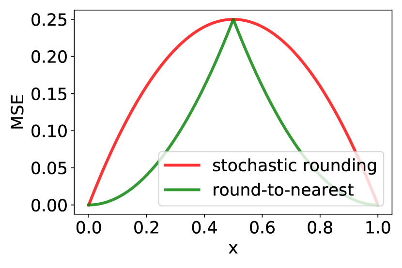
(a)

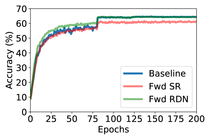
(b)

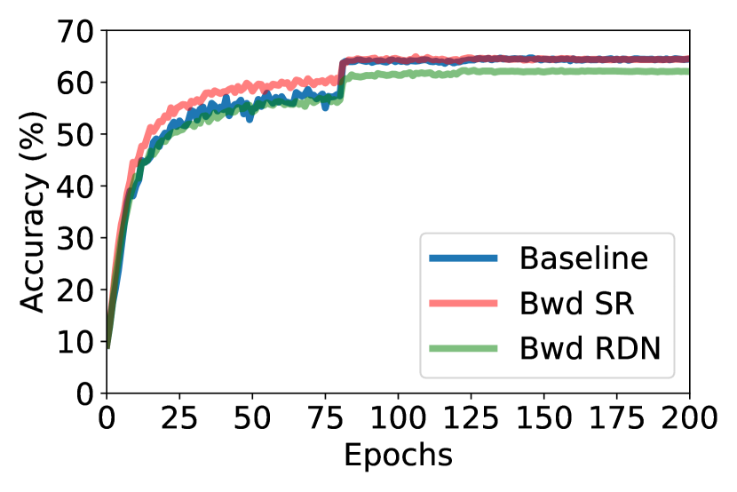
(c)

Figure 1: Comparison between stochastic rounding (SR) and round-to-nearest (RDN) quantization. In (a) we present the MSE of a uniform distributed tensor with the two different rounding schemes. Quantization to 4 bits of the forward phase (b) and backward phase (c) of ResNet18 - Cifar100 dataset with SR and RDN. While MSE is important in the forward phase, unbiasness achieved with SR is crucial for the backward phase. The bwd and fwd in (b) and (c) respectively, are in full precision to focus on the effect of the rounding scheme only in one pass of the network in each experiment.

3.2 Background: When is it important to use unbiased quantization?

To prove convergence, textbook analyses of SGD typically assume the expectation of the (mini-batch) weight gradients is sufficiently close to the true (full-batch) gradient (e.g., assumption 4.3 in [6]). This assumption is satisfied when the weight gradients are unbiased. Next, we explain (as pointed out by previous works, such as [7]) that the weight gradients are unbiased when the neural gradients are quantized stochastically without bias.

Denote $W_{l}$ as the weights between layer $l-1$ and $l$, $C$ the cost function, and $f_{l}$ as the activation function at layer $l$. Given an input–output pair $(x,y)$, the loss is:

$$C\left(y,f_{L}\left(W_{L}f_{L-1}\left(W_{L-1}\cdots f_{2}\left(W_{2}f_{1}\left(W_{1}x\right)\right)\cdots\right)\right)\right)\,.$$ (10)

Backward pass. Let $z^{l}$ be the weighted input (pre-activation) of layer $l$ and denote the output (activation) of layer $l$ by $a_{l}$. The derivative of the loss in terms of the inputs is given by the chain rule:

$$\delta_{l}\triangleq\frac{dC}{dz_{l}}=\frac{da_{l}}{dz_{l}}\cdots\frac{dz_{L-1}}{da_{L-2}}\cdot\frac{da_{L-1}}{dz_{L-1}}\cdot\frac{dz_{L}}{da_{L-1}}\cdot\frac{da_{L}}{dz_{L}}\cdot\frac{dC}{da_{L}}\,.$$ (11)

Therefore, $\delta_{L}\triangleq\frac{da_{L}}{dz_{L}}\cdot\frac{dC}{da_{L}}$, and we can write recursively the backprop rule $\forall l<L$:

$$\delta_{l}\triangleq\frac{da_{l}}{dz_{l}}\frac{dz_{l+1}}{da_{l}}\cdot\delta_{l+1}\,.$$ (12)

In its quantized version, $\delta_{L}^{q}=Q\left(\delta_{L}\right)$, and Eq. 12 has the following form (with ReLU activations):

$$\delta_{l}^{q}\triangleq Q\left(\frac{da_{l}}{dz_{l}}\frac{dz_{l+1}}{da_{l}}\delta_{l+1}^{q}\right)\,.$$ (13)

Assuming $Q(x)$ is an unbiased stochastic quantizer with $E[Q(x)]=x$, we next show the quantized backprop $\delta_{l}^{q}$ is an unbiased approximation of backprop:

$$\begin{split}E\delta_{l}^{q}&=EQ\left(\frac{da_{l}}{dz_{l}}\frac{dz_{l+1}}{da_{l}}\delta_{l+1}^{q}\right)\overset{\left(1\right)}{=}E\left[E\left[Q\left(\frac{da_{l}}{dz_{l}}\frac{dz_{l+1}}{da_{l}}\delta_{l+1}^{q}\right)|\delta_{l+1}^{q}\right]\right]\\ &\overset{\left(2\right)}{=}E\left[\frac{da_{l}}{dz_{l}}\frac{dz_{l+1}}{da_{l}}\delta_{l+1}^{q}\right]\overset{\left(3\right)}{=}\frac{da_{l}}{dz_{l}}\frac{dz_{l+1}}{da_{l}}E\delta_{l+1}^{q}\overset{\left(4\right)}{=}\frac{da_{l}}{dz_{l}}\frac{dz_{l+1}}{da_{l}}\delta_{l}\,,\end{split}$$ (14)

where in (1) we used the law of total expectation, in (2) we used $E[Q(x)]=x$, in (3) we used the linearity of back-propagation, and in (4) we assumed by induction that $E\left[\delta_{l+1}\right]=\delta_{l+1}^{q}$, which holds initially: $E\delta_{L}^{q}=EQ\left({\delta_{L}}\right)=\delta_{L}$. Finally, the gradient of the weights in layer $l$ is $\nabla_{W_{l}}C=\delta_{l}a_{l-1}^{\top}$ and its quantized form is $\nabla_{W_{l}}C_{q}=\delta_{l}^{q}a_{l-1}^{\top}$. Therefore, the update $\nabla_{W_{l}}C_{q}$ is an unbiased estimator of $\nabla_{W_{l}}C$:

$$\begin{split}E\left[\nabla_{W_{l}}C_{q}\right]&=E\left[\delta_{l}^{q}a_{l-1}^{\top}\right]=E\left[\delta_{l}^{q}\right]a_{l-1}^{\top}=\delta_{l}a_{l-1}^{\top}=\nabla_{W_{l}}C\,.\end{split}$$ (15)

Forward pass. The forward pass is different from the backward pass in that unbiasedness at the tensor level is not necessarily a guarantee of unbiasedness at the model level since the activation functions and loss function are not linear. For example, suppose we have two weight layers $W_{1},W_{2}$, activation $f$, input $x$, and the SR quantizer $Q$. Then, despite that $Q$ is unbiased (i.e., $EQ(x)=x$), we get:

$$\mathbb{E}[f(W_{2}Q(f(W_{1}x))]\neq\mathbb{E}[f(W_{2}(f(W_{1}x))]$$ (16)

since $f$ is non-linear. This means there is no point to use SR in the forward path, since it will increase the MSE (Eq. 9), but it will not fix the bias issue.

3.3 Conclusions: when to use each quantization scheme?

As we explained in section 3.2, unbiased neural gradients quantization leads to an unbiased estimate of the weight gradients, which enables proper convergence of SGD [6]. Thus, bias in the gradients can hurt the performance and should be avoided, even at the cost of increasing the MSE. Therefore, neural gradients, should be quantized using SR, following subsection 3.2. However, the forward phase should be quantized deterministically (using RDN) since stochastic rounding will not make the loss estimate unbiased due to the non-linearity of the loss and activation functions (e.g., Eq. 16) while unnecessarily increasing the MSE (as shown in Eq. 9), an increase which typically harms the final accuracy. In Figs. 1(b) and 1(c) we see that these theoretical observations are consistent with empirical observations favoring RDN for the forward pass and SR for the backward pass.

4 LUQ - a logarithmic unbiased quantizer

A recent work [9] showed that the neural gradients can be approximated with the lognormal distribution, and showed analytically that the optimal FP4 format is [1,3,0]. However, they were not able to successfully quantize to this format (their narrowest format was FP5). Following their work and the conclusions from previous section, we aim to create, for the first time, a Logarithmic Unbiased Quantizer (LUQ).

Standard radix-2 floating-point defines a dynamic range. In standard FP, all the values below the minimum FP representation are pruned to 0 and all the values above the maximum FP representation are clipped to the maximum. In order to create a fully unbiased quantizer, we need to keep all the following three regions unbiased: below range minimum, inside range, and above range maximum.

Below FP minimum: Stochastic underflow

Given an underflow threshold $\alpha$ we define a stochastic pruning operator, which prunes a given value $x$, as

$$T_{\alpha}\left(x\right)=\begin{cases}x&\quad\mathrm{,if}$ $|x|\geq\alpha\\ \text{sign}(x)\cdot\alpha&\quad w.p.\,\,\,\frac{|x|}{\alpha},\mathrm{if}$ $|x|<\alpha\\ 0&\quad w.p.\,\,\,1-\frac{|x|}{\alpha},\mathrm{if}$ $|x|<\alpha\,.\end{cases}$$ (17)

Above FP maximum: Underflow threshold

In order to create an unbiased quantizer, the largest quantization value $2^{b-1}\alpha$ should avoid clipping any values in a tensor $x$, otherwise this will create a bias. Therefore, the maximal quantization value is chosen as $\max(|x|)$, the minimal value which will avoid clipping and bias. Accordingly, the underflow threshold $\alpha$ is (with $b=3$ for FP4)

$$\alpha=\frac{\text{max}(|x|)}{2^{2^{b-1}}}\,.$$

Inside FP range: Unbiased FP quantizer

Given an underflow threshold $\alpha$, let $Q_{\alpha}(x)$ be a FP round-to-nearest $b$-bits quantizer with bins $\{\alpha,2\alpha,...,2^{b-1}\alpha\}$. Assume, without loss of generality, $2^{n-1}\alpha<x<2^{n}\alpha$ $(n\in\{0,1...,b-1\})$ . We will use the following quantizer, which is a special case of SR (Eq. 1), and is unbiased as a special case of Eq. 2.:

$$Q_{\alpha}(x)=\begin{cases}2^{n-1}\alpha&w.p.\,\,\,\frac{2^{n}\alpha-x}{2^{n}\alpha-2^{n-1}\alpha}\\ 2^{n}\alpha&w.p.\,\,\,1-\frac{2^{n}\alpha-x}{2^{n}\alpha-2^{n-1}\alpha}=\frac{x-2^{n-1}\alpha}{2^{n-1}\alpha}\,.\end{cases}$$ (18)

Logarithmic rounding

The naive implementation of stochastic rounding can be expensive, since it cannot use the standard quantizer. Traditionally, in order to use the standard quantizer the implementation includes simply adding uniform random noise $\epsilon\sim U[-\frac{2^{n-1}\alpha}{2},\frac{2^{n-1}\alpha}{2}]$ to $x$ and then using a round-to-nearest operation. The overhead of such stochastic rounding is typically negligible [13] in comparison to other operations in neural networks training. Moreover, it is possible to reduce any such overhead with the re-use of the random samples (Section A.2.1). In our case, in order to implement a logarithmic round-to-nearest, we need to correct an inherent bias since $\alpha\cdot 2^{\lfloor{\log\left(\frac{|x|}{\alpha}\right)\rceil}}\neq\alpha\cdot\lfloor 2^{\log\left(\frac{|x|}{\alpha}\right)}\rceil$.

For a bin $[2^{n-1},2^{n}]$, the midpoint $x_{m}$ is

$$x_{m}=\frac{2^{n}+2^{n-1}}{2}=\frac{3}{4}\cdot 2^{n-1}\,.$$ (19)

Therefore, we can apply round-to-nearest-power (RDNP) directly on the exponent $x$ of any value $2^{n-1}\leq 2^{x}\leq 2^{n}$ as follows:

$$\begin{split}\text{RDNP}(2^{x})&=2^{\lfloor\log{\left(\frac{4}{3}\cdot 2^{x}\right)\rfloor}}=2^{\lfloor x+\log{\left(\frac{4}{3}\right)}\rfloor}=2^{\text{RDN}\left(x+\log{\left(\frac{4}{3}\right)}-\frac{1}{2}\right)}\approx 2^{\text{RDN}\left(x-0.084\right)}\,.\end{split}$$ (20)

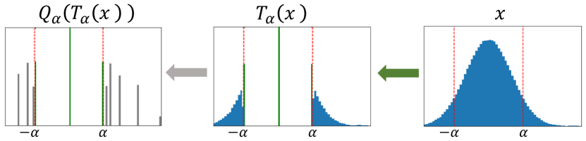
Figure 2: The effect of LUQ on the neural gradients. Histograms are for one layer of ResNet18 Cifar100 dataset, with the underflow threshold $\alpha$ (red dashed line). The first step (green arrow) represents stochastic underflow (Eq. 23) on the neural gradient. The second step (grey arrow) represents the logarithmic stochastic rounding step (Eq. 18), that quantizes all the values $|x|>\alpha$.

Logarithmic unbiased quantization (LUQ)

LUQ, the quantization method we suggested above, is unbiased, since it can be thought of applying logarithmic stochastic rounding (Eq. 18) on top of stochastic pruning (Eq. 23)

$$X_{q}=Q_{\alpha}\left(T_{\alpha}(x)\right)\,.$$ (21)

Since $T_{\alpha}$ and $Q_{\alpha}$ are unbiased, $X_{q}$ is an unbiased estimator for $x$, from the law of total expectation,

$$\begin{split}E[X_{q}]&=E\left[Q_{\alpha}\left(T_{\alpha}(x)\right)\right]=E\left[E\left[Q_{\alpha}\left(T_{\alpha}(x)\right)\right]|T_{\alpha}(x)\right]=E\left[T_{\alpha}(x)\right]=x\,,\end{split}$$ (22)

where the expectation is over the randomness of $T_{\alpha}$ and $Q_{\alpha}$. In Fig. 2 we show an illustration of LUQ. The first step includes stochastic pruning for the values below the pruning threshold ($|x|<\alpha$). The second step includes the logarithmic quantization with format FP4 of the values above the pruning threshold ($|x|>\alpha$). In Fig. 3 we show an ablation study of the effect of the different parts of LUQ on ResNet50 ImageNet dataset—while standard FP4 diverges, adding stochastic pruning or round-to-nearest-power enables convergence, but with significant degradation. Combining both methods improves the results. Finally, the best results are obtained using the suggested LUQ method, which includes additionally the suggested underflow threshold choice as the optimal unbiased value.

4.1 SMP: Reducing the variance while keeping it unbiased

In the previous section, we presented an unbiased method for logarithmic quantization of the neural gradients called LUQ. Following the bias-variance decomposition, if the gradients are now unbiased, then the only remaining issue should be their variance. Therefore, we suggest a method to reduce the quantization variance by repeatedly sampling from the stochastic quantizers in LUQ, and averaging the resulting samples of the final weight gradients. The different samples can be calculated in parallel, so the only overhead on the network throughput will be the averaging operation. The power overhead will be approximately $\sim\frac{1}{3}$ of the number of additional samples, since it affects only in the update GEMM (Eq. 27). For $N$ different samples, the proposed method will reduce the variance by a factor of $\frac{1}{N}$, without affecting the bias [15]. In Fig. 3 we show the effect of the different number of samples (SMP) on 2-bit quantization of ResNet18 Cifar100 dataset. There, we achieve with 16 samples accuracy similar to a full-precision network. This demonstrates that the variance is the only remaining issue in neural gradient quantization using LUQ, and that the proposed averaging method can erase this variance gap, with some overhead.

4.2 FNT: Fine-tuning in high precision

After the 4-bit training is finished, we suggest to reduce the gap from the full precision model, by running $T$ additional iterations in which we increase all the network parts to higher precision, except the weights which remain in low precision. We noticed that with this scheme we get the best accuracy for the fine-tuned network. At inference time the activations and weights are quantized to lower precision. During the fine-tune phase, the Learning Rate (LR) is increased linearly during $\frac{T}{2}$ iterations and then reduced linearly with the same slope:

$$\text{LR}_{t}=\begin{cases}\text{LR}_{T}+\frac{(\text{LR}_{\text{base}}-\text{LR}_{T})}{T/2}&\quad\mathrm{,if}$ $t\leq\frac{T}{2}\\ \text{LR}_{T}\cdot\frac{(T-t)}{T/2}&\quad\mathrm{,else}\end{cases}\,,$$ (23)

where $\text{LR}_{T}$ is the final LR of the 4-bit training and $\text{LR}_{\mathrm{base}}$ is the maximal LR of the fine-tune phase.

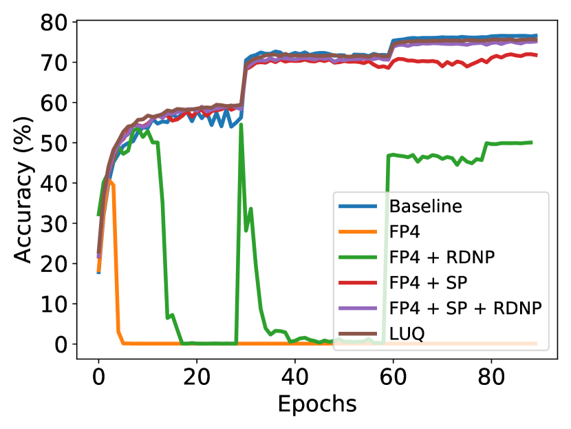
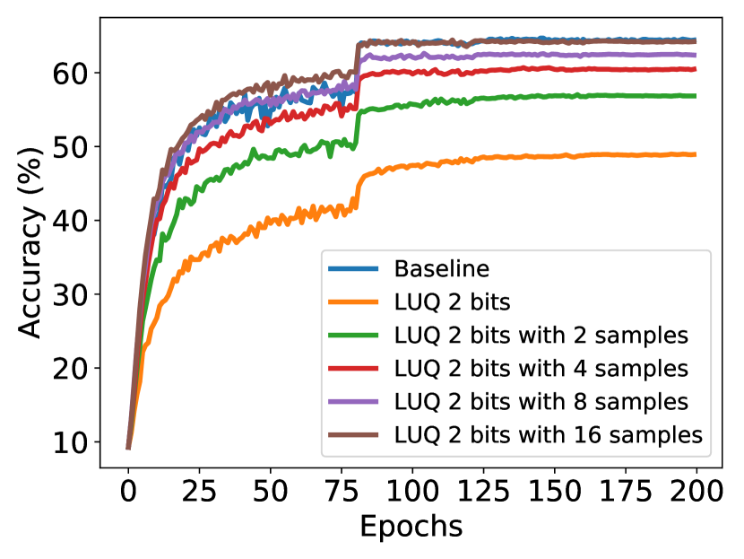
Figure 3: (Left): ResNet50 top-1 validation accuracy in ImageNet dataset with different quantization schemes for the neural gradients. SP refers to stochastic pruning (Eq. 23). RDNP refers to round-to-nearest-power (Eq. 20). Notice that with the suggested LUQ we are able to almost close the degradation from baseline. (Right): ResNet18 top-1 validation accuracy in CIFAR100 with quantization of the neural gradients to 2-bit (FP2 - [1,1,0] format) using different samples numbers to reduce the variance. Notice that 16 samples completely close the gap to the baseline.

4.3 Implementation details

Reducing the data movement

So far, we focused on resolving the 4-bit GEMM operation bottleneck in DNNs training. It reduces not only the computational resources for the GEMM operations, but also reduces the required memory in DNNs training. However, LUQ, similarly to previous quantization methods [23, 11, 10], requires a statistical measurement of the tensor to define the quantization dynamic range. Specifically, LUQ requires a measurement of the maximum of the neural gradient tensor. Such measurement increases the data movement from and to memory, making this data movement a potential bottleneck.

In order to avoid this bottleneck, we combined in LUQ the In-hindsight [14] statistics estimation, which use a pre-computed measurement to quantize the current tensor and in parallel extract the current statistics for the next iteration. The maximum estimate in LUQ, $\hat{m}$ is calculated as:

$$\hat{m}^{t}=(1-\eta)\cdot\text{max}(|x^{t-1}|)+\eta\cdot\hat{m}^{t-1}\,,$$ (24)

where $\eta$ is the momentum hyperparameter, and $x$ is tensor of neural gradients. In Section A.2.3 we show the effectiveness of this statistics estimation, which eliminates this data movement bottleneck, with a negligible change to the accuracy.

Forward pass quantization

INT4 quantization methods for the weights and activations (forward pass) were well studied in the past. In this paper we combined the proposed LUQ to quantize the neural gradients (FP4) with SAWB [10] to quantize the forward pass (INT4). SAWB determines the quantization scaling factor by first finding the optimal (in term of MSE) scaling factor on six distribution approximations of the true tensor distribution, and then apply linear regression to find the chosen scaling factor. Additional details appears in [10].

Training time measurement

Notice that, currently, AI accelerators do not support 4-bit formats for training. This means that we can only simulate the quantization process, but are not able to actually measure training time or memory reduction. This is the common practice in the neural network quantization literature, where the algorithms often appear before the hardware that can support them. For example, though we can find FP8 training publications since 2019 [22], only recently did Nvidia announce their first GPU that supports the FP8 format (H100).

5 Experiments

In this section, we evaluate the proposed LUQ for 4-bit training on various DNN models. For all models, we use their default architecture, hyper-parameters, and optimizers combined with a custom-modified Pytorch framework that implemented all the low precision schemes. Additional experimental details appear in Section A.1.

Main results

In Table 1 we show the top-1 accuracy achieved in 4-bit training using LUQ to quantizing the neural gradients to FP4 and combined with a previously suggested method, SAWB [10], to quantize the weights and activations to INT4. We compare our method with Ultra-low [23] showing better results in all the models, achieving SOTA in 4-bit training. Moreover, we improve the results by using the proposed SMP (Section 4.1). In Table 2 we show the effect of the proposed fine-tuning, reducing or closing completely the gap from full-precision model. We verified that stochasticity has only a negligible on the variance of final performance by running a few different seeds. Additional experiments appears in Section A.2.

Table 1: Comparison of 4-bit training of the proposed method LUQ with Ultra-low [23] in various vision models with ImageNet dataset, Transformer-base in WMT En-De task dataset and BERT fine-tune in SQUAD dataset. SMP refers to doing two samples of the SR quantization of neural gradients in order to reduce the variance (Section 4.1).

Model	Baseline	Ultra-low [23]	LUQ	LUQ + SMP
ResNet-18	69.7 %	68.27%	69.12%	69.24 %
ResNet-50	76.5%	74.01%	75.4 %	75.63 %
MobileNet-V2	71.9 %	68.85 %	69.59 %	69.7 %
ResNext-50	77.6 %	N/A	75.91 %	76.02 %
Transfomer-base	27.5 (BLEU)	25.4	27.17	27.25
BERT fine-tune	87.03 (F1)	N/A	85.77	85.9

Overhead of SMP and FNT

We limit our experiments with the proposed SMP method to only two samples. This is to achieve a similar computational overhead as Ultra-low[23], with their suggested two-phase-rounding (TPR) which also generates a duplication for the neural gradient quantization. Additional ablation study of the SMP overhead appears in Section A.2. The throughput of a 4-bit training network is approximately 8x in comparison to FP-16 training [23]. This means that doing one additional epoch in high precision reduces the throughput by $\sim 8\%$ . In comparison, Ultra-low [23] does full-training with all the 1x1 convolutions in 8bit, which reduces the throughput by $\sim 50\%$ in comparison to all 4bit training.

Table 2: Effect of the proposed FNT method (Section 4.2) using FP16 format with different epochs.

Model	Baseline	LUQ + SMP	+FNT 1 epoch	+FNT 2 epochs	+FNT 3 epochs
ResNet-18	69.7 %	69.27 %	69.7 %	-	-
ResNet-50	76.5 %	75. 63%	75.89 %	76 %	76.18 %
MobileNet-V2	71.9 %	69.7 %	70.1 %	70.3 %	70.3 %
ResNext-50	77.6 %	76.02%	76.25 %	76.33 %	76.7 %

Forward-backward ablations

In Table 4 we show the top-1 accuracy in ResNet50 with different quantization schemes. The forward phase (activations + weights) is quantized to INT4 with SAWB [10] and the backward phase (neural gradients) to FP4 with LUQ. As expected, the network is more sensitive to the quantization of the backward phase.

6 Discussion

Conclusions

In this work, we analyze the difference between two rounding schemes: round-to-nearest and stochastic-rounding. We showed that, while the former has lower MSE and works better for the quantization of the forward phase (weights and activations), the latter is an unbiased approximation of the original data and works better for the quantization of the backward phase (specifically, the neural gradients). Based on these conclusions, we propose a logarithmic unbiased quantizer (LUQ) to quantize the neural gradients to format FP4 [1,3,0]. Combined with a known method for quantizing the weights and activations to INT4 we achieved, without overhead, state-of-the-art in standard format 4-bit training in all the models we examined, e.g., 1.1% error in ResNet50 vs. 2.49% for the previous known SOTA ([23], which used non-standard format). Moreover, we suggest two more methods to improve the results, with overhead comparable to [23]. The first reduces the quantization variance, without affecting the unbiasedness of LUQ, by averaging several samples of stochastic neural gradients quantization. The second is a simple method for fine-tuning in high precision for one epoch. Combining all these methods, we were able for the first time to achieve 0.32% error in 4-bit training of ResNet50 ImageNet dataset.

Multiplication free backpropagation

In this work, we reduce the GEMM bottleneck by combining two different data-types for the forward (INT4) and backward (FP4) passes. Standard GEMMs operations with different formats, requires to cast the operand to a common datatype before the multiplication. The cost of the casting operation can be significant. We notice, that we are dealing with a special case, where one of the operand include only mantissa (weights and activations) and the other only exponent (neural gradients). Our initial analysis, show that this allow with small hardware changes, to reduce the area of standard GEMM block by 5x. Additional details appears in Section A.4

Accumulation width

A different future direction is to reduce the accumulator width, which is usually kept as FP32. As explained in Section A.4, the FP32 accumulator is the most expensive block when training in low bits. Now, after allowing training with 4-bit it is reasonable to think that the accumulator width can be reduced.

Appendix A Appendix

A.1 Experiments details

In all our experiments we use the most common approach [3, 11] for quantization where a high precision of the weights are kept and quantized on-the-fly. The updates are done in full precision. In all our experiments we use 8 GPU GeForce Titan Xp or GeForce RTX 2080 Ti or Ampere A40.

ResNet / ResNext

We run the models ResNet-18, ResNet-50 and ResNext-50 from torchvision. We use the standard pre-processing of ImageNet ILSVRC2012 dataset. We train for 90 epochs, use an initial learning rate of 0.1 with a 0.1 decay at epochs 30,60,80. We use standard SGD with momentum of 0.9 and weight decay of 1e-4. The minibatch size used is 256. Following the DNNs quantization conventions [3, 19, 11] we kept the first and last layer (FC) at higher precision. Additionally, similar to [23] we adopt the full precision at the shortcut which constitutes only a small amount of the computations ($\sim 1\%$). We totally The "underflow threshold" in LUQ is updated in every bwd pass as part of the quantization of the neural gradients. In all experiments, the BN is calculated in high-precision. The hindsight momentum is $\eta=0.1$ and in the FNT experiments we use $\text{lr}_{base}=1e-3$.

MobileNet V2

We run Mobilenet V2 model from torchvision. We use the standard pre-processing of ImageNet ILSVRC2012 dataset. We train for 150 epochs, use an initial learning rate of 0.05 with a cosine learning scheduler. We use standard SGD with momentum of 0.9 and weight decay of 4e-5. The minibatch size used is 256. Following the DNNs quantization conventions [3, 19, 11] we kept the first and last layer (FC) at higher precision. Additionally, similar to [23] we adopt the full precision at the depthwise layer which constitutes only a small amount of the computations ($\sim 3\%$). The "underflow threshold" in LUQ is updated in every bwd pass as part of the quantization of the neural gradients. In all experiments, the BN is calculated in high-precision.

Transformer

We run the Transformer-base model based on the Fairseq implementation on the WMT 14 En-De translation task. We use the standard hyperparameters of Fairseq including Adam optimizer. We implement LUQ over all attention and feed forwards layers.

A.2 Additional experiments

A.2.1 Stochastic rounding amortization

As explained in Section 4 usually the overhead of the stochastic rounding is typically negligible in comparison to other operation in neural network training. However, to reduce even more this overhead, is it possible to re-use the random samples. In Fig. 4 we show the effect of such re-using that does not change the network accuracy.

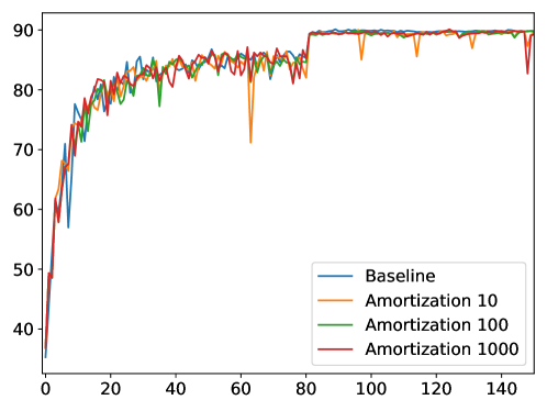
Figure 4: ResNet18 top-1 validation in Cifar10 dataset, with 4-bit quantization of the neural gradients using stochastic-rounding. The amortization is the numbers of iteration that we re-use the random samples.

A.2.2 SMP overhead

The SMP method (Section 4.1) has a power overhead of $\sim\frac{1}{3}$ of the number of additional samples since it influences only the update GEMM. In Fig. 5 we compare LUQ with one additional sample which has $\sim 33\%$ power overhead with regular LUQ with additional $\sim 33\%$ epochs. The lr scheduler was expanded respectively. We can notice that even both methods have similar overhead the variance reduction achieved with SMP is more important for the network accuracy than increasing the training time.

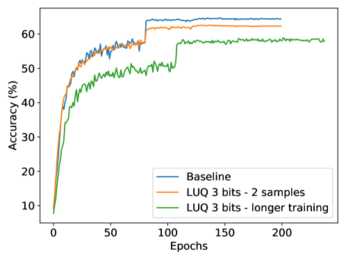
Figure 5: Comparison of ResNet-18 3 bit training on Cifar100 dataset of LUQ with 2 samples with longer training of regular LUQ. Both methods have similar overhead, but the SMP method leads to better accuracy.

A.2.3 Data movement reduction effect

LUQ requires the measurement of the maximum to choose the underflow threshold $\alpha$ (Section 4). This measurement can create a data movement bottleneck. In order to avoid it, we combine in LUQ the proposed maximum estimation of Hindsight [14], which use previous iterations statistics. In Fig. 6 we compate between the measured maximum and the Hindsight estimation, showing they can similar value. Moreover in Table 3 we show that the effect of the Hindsight estimation on the network accuracy is negligible while completely eliminating the data movement bottleneck.

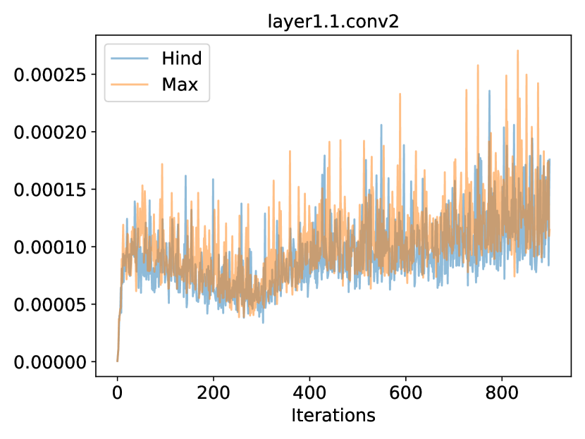
(a)

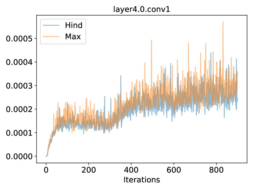
(b)

Figure 6: Measured maximum and hindsight [14] maximum estimation in two different layers of ResNet18 ImageNet dataset. As you can notice, the hindsight estimation is close to the measured maximum and reduce completely the data movement bottleneck

Table 3: Effect of applying Hindsight maximum estimation on the network accuracy

Model	LUQ	LUQ + Hindsight [14]
ResNet18	69.09	69.12
ResNet50	75.42	75.4

Table 4: ResNet-50 accuracy with ImageNet dataset while quantization different parts of the network. The forward phase is quantized to INT4 format with SAWB [10] while the backward phase is quantized with the proposed LUQ. As expected, the quantization of the backward phase makes more degradation to the network accuracy.

Forward	Backward	Accuracy
FP32	FP32	76.5 %
INT4	FP32	76.35 %
FP32	FP4	75.6 %
INT4	FP4	75.4 %

A.3 Comparison to [23]

Floating point radix conversion requires an explicit multiplication and may require additional non-standard hardware support [17]. Specifically, [23] requires a conversion from the radix-2 FP32 to a radix-4 FP4 of the neural gradients. They show this conversion requires the multiplication by the constant 1.6.

Notice that it is not possible to convert between radix floating point formats by a fixed shift. For example, suppose we first convert the radix-2 FP32 to radix-2 FP4 and then shift the exponent (where the shift is equivalent to multiplication by 2). This would lead to an incorrect result, as we show with a simple example: let us assume radix-2 quantization with bins 1,2,4,8 and radix-4 quantizations with bins 1,4,16,64. For the number 4.5, if we quantize it first to radix-2 we get the quantized number 4, then we multiply it by 2 we get 8. In contrast, radix-4 quantization should give the result 4.

In contrast, our proposed method, LUQ, uses the standard radix-2 format and does not require non-standard conversions. The use of standard hardware increases the benefit of the low bits quantization.

A.4 MF-BPROP: multiplication free backpropagation

The main problem of using different datatypes for the forward and backward phases is the need to cast them to a common data type before the multiplication during the backward and update phases. In our case, the weights ($W$) and pre-activations ($z$) are quantized to INT4 while the neural gradients ($\frac{\partial C}{\partial z}$) to FP4, where $C$ represent the loss function, $f$ a non-linear function and $a$ the post-activation. During the backward and update phases, in each layer $l$ there are two GEMMs between different datatypes:

$$\textbf{[Forward]}\quad z_{l}=W_{l}a_{l-1}\quad\quad a_{l}=f(z_{l})$$ (25)

$$\textbf{[Backward]}\quad\frac{\partial C}{\partial z_{l-1}}=\text{Diag}(f^{\prime}(z_{l-1}))W_{l}^{T}\frac{\partial C}{\partial z_{l}}$$ (26)

$$\textbf{[Update]}\quad\frac{\partial C}{\partial W_{l}}=\frac{\partial C}{\partial z_{l-1}}a_{l}^{T}$$ (27)

Regularly, to calculate these GEMMs there is a need to cast both data types to a common data type (in our case, FP7 [1,4,2]), then do the GEMM and finally, the results are usually accumulated in a wide accumulator (Fig. 7(a)). This casting cost is not negligible. For example, casting INT4 to FP7 consumes $\sim 15\%$ of the area of an FP7 multiplier.

In our case, we are dealing with a special case where we do a GEMM between a number without mantissa (neural gradient) and a number without exponent (weights and activations), since INT4 is almost equivalent to FP4 with format [1,0,3]. We suggest transforming the standard GEMM block (Fig. 7(a)) to Multiplication Free BackPROP (MF-BPROP) block which contains only a transformation to standard FP7 format (see Fig. 7(b)) and a simple XOR operation. More details on this transformation appear in Section A.4.1. In our analysis (Section A.4.2) we show the MF-BPROP block reduces the area of the standard GEMM block by 5x. Since the FP32 accumulator is still the most expensive block when training with a few bits, we reduce the total area in our experiments by $\sim 8\%$. However, as previously showed [24] 16-bits accumulators work well with 8-bit training, so it is reasonable to think, it should work also with 4-bit training. In this case, the analysis (Section A.4.2) shows that the suggested MF-BPROP block reduces the total area by $\sim 22\%$.

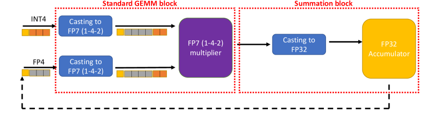
(a)

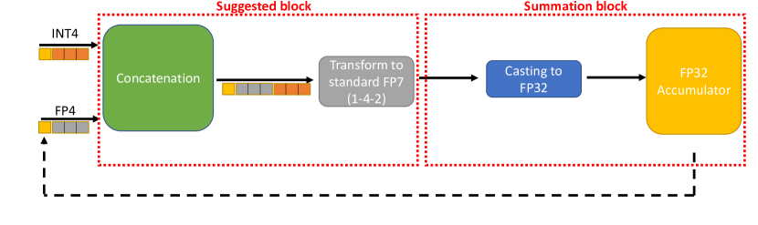
(b)

Figure 7: (a): Standard MAC block illustration containing the two main blocks - one for GEMM and second for accumulator. The GEMM block for hybrid datatype as in our case (FP4 and INT4) requires a casting to a common datatype before being inserted into the multiplier. (b): The suggested MAC block, which replace the multiplier with the proposed MF-BPROP. Instead of doing an expensive casting followed by a multiplication, we propose to make only a simple XOR and a transformation (Section A.4.1) reducing the GEMM area by 5x (Section A.4.2).

A.4.1 Transform to standard fp7

We suggest a method to avoid the use of an expensive GEMM block between the INT4 (activation or weights) and FP4 (neural gradient). It includes 2 main elements: The first is a simple xor operation between the sign of the two numbers and the second is a transform block to standard FP7 format. In Fig. 8 we present an illustration of the proposed method. The transformation can be explained with a simple example: for simplicity, we avoid the sign which requires only xor operation. The input arguments are 3 (011 bits representation in INT4 format) and 4 (011 bits representation in FP4 1-3-0 format). The concatenation brings to the bits 011 011. Then looking at the table in the input column where the M=3 (since the INT4 argument = 3) and get the results in FP7 format of 0100 10 ( = E+1 2) which is 12 in FP7 (1-4-2) as the expected multiplication result.

In the next section, we analyze the area of the suggested block in comparison to the standard GEMM block, showing a 5x area reduction.

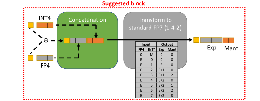
Figure 8: Illustration of MF-BPROP block which replaces a standard multiplication. It includes: (1) a simple xor operation between the sign. (2) A transform to standard FP7 format. We present the table to make this transform - E and M represent the bits of the FP4 and INT4 respectively without the sign. Exp and Mant are the bits of the output exponent (4-bit) and mantissa (2-bit) of the output in FP7 format.

A.4.2 Backpropagation without multiplcation analysis

In this section, we show a rough estimation of the logical area of the proposed MF-BPROP block which avoids multiplication and compares it with the standard multiplier. In hardware design, the logical area can be a good proxy for power consumption [16]. Our estimation doesn’t include synthesis optimization. In Table 5 we show the estimation of the number of gates of a standard multiplier, getting 264 logical gates while the proposed MF-BPROP block has an estimation of 49 gates (Table 6) achieving a $\sim 5x$ area reduction. For fair comparison we remark that in the proposed scheme the FP32 accumulator is the most expensive block with an estimation of 2453 gates, however we believe it can be reduced to a narrow accumulator such as FP16 (As previously shown in [24] which have an estimated area of 731 gates. In that case, we reduce the total are by $\sim 22\%$.

Table 5: Rough estimation of the number of logical gates for a standard GEMM block which contain two blocks: a casting to FP7 and a FP7 multiplier.

Block	Operation	# Gates
Casting to FP7	Exponent 3:1 mux	12
	Mantissa 4:1 mux	18
FP7 [1,4,2] multiplier	Mantissa multiplier	99
	Exponent adder	37
	Sign xor	1
	Mantissa normalization	48
	Rounding adder	12
	Fix exponent	37
Total		264

Table 6: Rough estimation of the number of logical gates for the proposed MF-BPROP block.

Block	Operation	# Gates
MF-BPROP	Exponent adder	30
	Mantissa 4:1 mux	18
	Sign xor	1
Total		49

References

- Alistarh et al. [2016] Dan Alistarh, Demjan Grubic, Jungshian Li, Ryota Tomioka, and M. Vojnovic. Qsgd: Communication-optimal stochastic gradient descent, with applications to training neural networks. 2016.
- Banner et al. [2019] R. Banner, Yury Nahshan, and Daniel Soudry. Post training 4-bit quantization of convolutional networks for rapid-deployment. In NeurIPS, 2019.
- Banner et al. [2018] Ron Banner, Itay Hubara, Elad Hoffer, and Daniel Soudry. Scalable methods for 8-bit training of neural networks. In NeurIPS, 2018.
- Bernstein et al. [2018] Jeremy Bernstein, Yu-Xiang Wang, Kamyar Azizzadenesheli, and Anima Anandkumar. signsgd: compressed optimisation for non-convex problems. ArXiv, abs/1802.04434, 2018.
- Bhalgat et al. [2020] Yash Bhalgat, Jinwon Lee, Markus Nagel, Tijmen Blankevoort, and Nojun Kwak. Lsq+: Improving low-bit quantization through learnable offsets and better initialization. 2020 IEEE/CVF Conference on Computer Vision and Pattern Recognition Workshops (CVPRW), pp. 2978–2985, 2020.
- Bottou et al. [2018] Léon Bottou, Frank E Curtis, and Jorge Nocedal. Optimization methods for large-scale machine learning. Siam Review, 60(2):223–311, 2018.
- Chen et al. [2020a] Jianfei Chen, Yu Gai, Zhewei Yao, Michael W Mahoney, and Joseph E Gonzalez. A statistical framework for low-bitwidth training of deep neural networks. arXiv preprint arXiv:2010.14298, 2020a.
- Chen et al. [2020b] Jianfei Chen, Yujie Gai, Z. Yao, M. Mahoney, and Joseph Gonzalez. A statistical framework for low-bitwidth training of deep neural networks. In NeurIPS, 2020b.
- Chmiel et al. [2021] Brian Chmiel, Liad Ben-Uri, Moran Shkolnik, E. Hoffer, Ron Banner, and Daniel Soudry. Neural gradients are lognormally distributed: understanding sparse and quantized training. In ICLR, 2021.
- Choi et al. [2018a] Jungwook Choi, P. Chuang, Zhuo Wang, Swagath Venkataramani, V. Srinivasan, and K. Gopalakrishnan. Bridging the accuracy gap for 2-bit quantized neural networks (qnn). ArXiv, abs/1807.06964, 2018a.
- Choi et al. [2018b] Jungwook Choi, Zhuo Wang, Swagath Venkataramani, P. Chuang, V. Srinivasan, and K. Gopalakrishnan. Pact: Parameterized clipping activation for quantized neural networks. ArXiv, abs/1805.06085, 2018b.
- Courbariaux et al. [2016] Matthieu Courbariaux, Itay Hubara, Daniel Soudry, Ran El-Yaniv, and Yoshua Bengio. Binarized Neural Networks: Training Deep Neural Networks with Weights and Activations Constrained to +1 or -1. arXiv e-prints, art. arXiv:1602.02830, February 2016.
- Croci et al. [2022] Matteo Croci, Massimiliano Fasi, Nicholas Higham, Theo Mary, and Mantas Mikaitis. Stochastic rounding: implementation, error analysis and applications. Royal Society Open Science, 9, 03 2022. doi: 10.1098/rsos.211631.
- Fournarakis & Nagel [2021] Marios Fournarakis and Markus Nagel. In-hindsight quantization range estimation for quantized training. 2021 IEEE/CVF Conference on Computer Vision and Pattern Recognition Workshops (CVPRW), pp. 3057–3064, 2021.
- Gilli et al. [2019] Manfred Gilli, Dietmar Maringer, and Enrico Schumann. Chapter 6 - generating random numbers. In Manfred Gilli, Dietmar Maringer, and Enrico Schumann (eds.), Numerical Methods and Optimization in Finance (Second Edition), pp. 103–132. Academic Press, second edition edition, 2019. ISBN 978-0-12-815065-8. doi: https://doi.org/10.1016/B978-0-12-815065-8.00017-0. URL https://www.sciencedirect.com/science/article/pii/B9780128150658000170.
- Iman & Pedram [1997] Sasan Iman and Massoud Pedram. Logic Synthesis for Low Power VLSI Designs. Kluwer Academic Publishers, USA, 1997. ISBN 0792380762.
- Kupriianova et al. [2013] Olga Kupriianova, Christoph Lauter, and Jean-Michel Muller. Radix conversion for ieee754-2008 mixed radix floating-point arithmetic. 2013 Asilomar Conference on Signals, Systems and Computers, Nov 2013. doi: 10.1109/acssc.2013.6810471. URL http://dx.doi.org/10.1109/ACSSC.2013.6810471.
- Liang et al. [2021] Tailin Liang, C. John Glossner, Lei Wang, and Shaobo Shi. Pruning and quantization for deep neural network acceleration: A survey. ArXiv, abs/2101.09671, 2021.
- Nahshan et al. [2019] Yury Nahshan, Brian Chmiel, Chaim Baskin, Evgenii Zheltonozhskii, Ron Banner, Alex M. Bronstein, and Avi Mendelson. Loss aware post-training quantization. arXiv preprint arXiv:1911.07190, 2019. URL http://arxiv.org/abs/1911.07190.
- Rastegari et al. [2016] Mohammad Rastegari, Vicente Ordonez, Joseph Redmon, and Ali Farhadi. Xnor-net: Imagenet classification using binary convolutional neural networks. In ECCV, 2016.
- Sakr & Shanbhag [2019] Charbel Sakr and Naresh R Shanbhag. Per-tensor fixed-point quantization of the back-propagation algorithm. 2019.
- Sun et al. [2019] Xiao Sun, Jungwook Choi, Chia-Yu Chen, Naigang Wang, Swagath Venkataramani, Vijayalakshmi Srinivasan, Xiaodong Cui, Wei Zhang, and Kailash Gopalakrishnan. Hybrid 8-bit floating point (hfp8) training and inference for deep neural networks. In NeurIPS, 2019.
- Sun et al. [2020] Xiao Sun, Naigang Wang, Chia-Yu Chen, Jiamin Ni, A. Agrawal, Xiaodong Cui, Swagath Venkataramani, K. E. Maghraoui, V. Srinivasan, and K. Gopalakrishnan. Ultra-low precision 4-bit training of deep neural networks. In NeurIPS, 2020.
- Wang et al. [2018] Naigang Wang, Jungwook Choi, Daniel Brand, Chia-Yu Chen, and K. Gopalakrishnan. Training deep neural networks with 8-bit floating point numbers. In NeurIPS, 2018.
- Wiedemann et al. [2020] Simon Wiedemann, Temesgen Mehari, Kevin Kepp, and W. Samek. Dithered backprop: A sparse and quantized backpropagation algorithm for more efficient deep neural network training. 2020 IEEE/CVF Conference on Computer Vision and Pattern Recognition Workshops (CVPRW), pp. 3096–3104, 2020.