3D-aware Image Synthesis via Learning Structural and Textural Representations
Supplementary Material

1 Overview

This supplementary material is organized as follows. Sec. 2 and Sec. 3 introduce the network structure and the training configurations used in VolumeGAN. Sec. 4 describes the details of implementing baseline approaches. Sec. 5 shows more qualitative results. We also attach a demo video (https://www.youtube.com/watch?v=p85TVGJBMFc) to show the continuous 3D control achieved by our VolumeGAN.

2 Network Structure

Recall that, our VolumeGAN first learns a feature volume with 3D CNN. The feature volume is then transformed into a feature field using a NeRF-like model. A 2D feature map is finally accumulated from the feature field and rendered to an image with a 2D CNN. Taking 256 resolution as an instance, we illustrate the architectures of these three models in Tab. 1, Tab. 2, and Tab. 3, respectively.

Table 1: Network structure for learning a feature volume as the structural representation. The output size is with order $\{C\times H\times W\times D\}$, where $D$ denotes the depth dimension.

Stage	Block	Output Size
input	Learnable Template	$256\times 4\times 4\times 4$
block1	$\left[\begin{array}[]{c}\text{3$\times$3$\times$3 $\mathtt{Conv}$, {128}}\\[-1.00006pt] \text{$\mathtt{AdaIN}$, {128}}\\[-1.00006pt] \text{$\mathtt{Upsample}$ }\\[-1.00006pt] \text{$\mathtt{LeakyReLU}$, 0.2}\end{array}\right]$	$128\times 8\times 8\times 8$
block2	$\left[\begin{array}[]{c}\text{3$\times$3$\times$3 $\mathtt{Conv}$, {64}}\\[-1.00006pt] \text{$\mathtt{AdaIN}$, {64}}\\[-1.00006pt] \text{$\mathtt{Upsample}$ }\\[-1.00006pt] \text{$\mathtt{LeakyReLU}$, 0.2}\end{array}\right]$	$64\times 16\times 16\times 16$
block3	$\left[\begin{array}[]{c}\text{3$\times$3$\times$3 $\mathtt{Conv}$, {32}}\\[-1.00006pt] \text{$\mathtt{AdaIN}$, {32}}\\[-1.00006pt] \text{$\mathtt{Upsample}$ }\\[-1.00006pt] \text{$\mathtt{LeakyReLU}$, 0.2}\end{array}\right]$	$32\times 32\times 32\times 32$

Table 2: Network structure of the generative feature field. The output size is with order $\{H\times W\times S\times C\}$, where $S$ is the number of sampling points along a certain camera ray. $\mathtt{FiLM}$ denotes the FiLM layer [4] and $\mathtt{Sine}$ stands for the Sine activation [6].

Stage	Block	Output Size
input	$-$	$64\times 64\times 12\times(32+3)$
mlp1	$\left[\begin{array}[]{c}\text{ $\mathtt{FC}$, {256}}\\[-1.00006pt] \text{$\mathtt{FiLM}$, {256}}\\[-1.00006pt] \text{$\mathtt{Sine}$}\end{array}\right]$	$64\times 64\times 12\times 256$
mlp2	$\left[\begin{array}[]{c}\text{ $\mathtt{FC}$, {256}}\\[-1.00006pt] \text{$\mathtt{FiLM}$, {256}}\\[-1.00006pt] \text{$\mathtt{Sine}$}\end{array}\right]$	$64\times 64\times 12\times 256$
mlp3	$\left[\begin{array}[]{c}\text{ $\mathtt{FC}$, {256}}\\[-1.00006pt] \text{$\mathtt{FiLM}$, {256}}\\[-1.00006pt] \text{$\mathtt{Sine}$}\end{array}\right]$	$64\times 64\times 12\times 256$
mlp4	$\left[\begin{array}[]{c}\text{ $\mathtt{FC}$, {256}}\\[-1.00006pt] \text{$\mathtt{FiLM}$, {256}}\\[-1.00006pt] \text{$\mathtt{Sine}$}\end{array}\right]$	$64\times 64\times 12\times 256$

Table 3: Network structure of the neural renderer, which renders a 2D feature map to a synthesized image. The output size is with order $\{C\times H\times W\}$.

Stage	Block	Output Size
input	$-$	$256\times 64\times 64$
block1	$\left[\begin{array}[]{c}\text{1$\times$ 1 $\mathtt{ModConv}$, {128}}\\[-1.00006pt] \text{$\mathtt{LeakyReLU}$, 0.2}\\[-1.00006pt] \text{1$\times$ 1 $\mathtt{ModConv}$, {128}}\\[-1.00006pt] \text{$\mathtt{Upsample}$ }\\[-1.00006pt] \text{$\mathtt{LeakyReLU}$, 0.2}\end{array}\right]$	$128\times 128\times 128$
block2	$\left[\begin{array}[]{c}\text{1$\times$ 1 $\mathtt{ModConv}$, {64}}\\[-1.00006pt] \text{$\mathtt{LeakyReLU}$, 0.2}\\[-1.00006pt] \text{1$\times$ 1 $\mathtt{ModConv}$, {64}}\\[-1.00006pt] \text{$\mathtt{Upsample}$ }\\[-1.00006pt] \text{$\mathtt{LeakyReLU}$, 0.2}\end{array}\right]$	$64\times 256\times 256$
RGB	3$\times$ 3 $\mathtt{Conv}$, 3	$3\times 256\times 256$

Table 4: Training configurations regarding different datasets.

Datasets	Fov	Rangedepth	$\#$Steps	Rangeh	Rangev	Sample_Dist	$\lambda$
CelebA	12	$[0.88,1.12]$	12	$[\pi/2-0.3,\pi/2+0.3]$	$[\pi/2-0.15,\pi/2+0.15]$	Gaussian	0.2
Cat	12	$[0.8,1.2]$	12	$[\pi/2-0.5,\pi/2+0.5]$	$[\pi/2-0.4,\pi/2+0.4]$	Gaussian	0.2
Carla	30	$[0.7,1.3]$	36	$[0,2\pi]$	$[\pi/2-\pi/8,\pi/2+\pi/8]$	Uniform	1
FFHQ	12	$[0.8,1.2]$	14	$[\pi/2-0.4,\pi/2+0.4]$	$[\pi/2-0.2,\pi/2+0.2]$	Gaussian	1
CompCars	20	$[0.8,1.2]$	30	$[0,2\pi]$	$[\pi/2-\pi/8,\pi/2+\pi/8]$	Uniform	1
Bedroom	26	$[0.7,1.3]$	40	$[\pi/2-\pi/8,\pi/2+\pi/8]$	$[\pi/2-\pi/10,\pi/2+\pi/10]$	Uniform	1

3 Training Configurations

Because of the wildly divergent data distribution, the training parameters vary greatly on different datasets. Tab. 4 illustrates the detailed training configuration of different datasets. Fov, Range_depth, and $\#$Steps are the field of view, depth range and the number of sampling steps along a camera ray. Range_h and Range_v denotes the horizontal and vertical angle range of the camera pose $\xi$. ’Sample_Dist’ denotes the sampling scheme of the camera pose. We only use Gaussian or Uniform sampling in our experiments. $\lambda$ is the loss weight of the gradient penalty.

4 Implementation Details of Baselines

HoloGAN [2]. We use the official implementation of HoloGAN. We train HoloGAN for 50 epochs. The generator of HoloGAN can only synthesize images in $64\times 64$ or $128\times$ resolution. We extend the generator with an extra $\mathtt{Upsample}$ and $\mathtt{AdaIN}$ block to synthesize $256\times 256$ images for comparison.

GRAF [5]. We use the official implementation of GRAF. We directly use the pre-trained checkpoints of CelebA and Carla provided by the authors. For the other datasets, we train GRAF with the same data and camera parameters as ours at the target resolution.

$\pi$-GAN [1]. We use the official implementation of $\pi$-GAN. We also directly use the pre-trained checkpoints of CelebA, Carla and Cat for comparison and retrain $\pi$-GAN models on the other three datasets, including FFHQ, CompCars and LSUN bedroom. The retrained models are progressively trained from a resolution of $32\times 32$ to $256\times 256$ following the official implementation.

GIRAFFE [3]. We use the official GIRAFFE implementation. GIRAFFE provides the pre-trained weights of FFHQ and CompCars in a resolution of $256\times 256$. The remaining datasets are also trained with the same camera distribution for a fair comparison.

5 Additional Results

Synthesis with front camera view. To better illustrate the 3D controllability, we show additional results of generating images with the front view. As shown in Fig. 1, the faces synthesized by VolumeGAN are more consistent with the given view, demonstrating a better 3D controllability.

Synthesis with varying camera views. Besides the front camera view, we also include a demo video (https://www.youtube.com/watch?v=p85TVGJBMFc), which shows more results with varying camera views. From the video, we can see the continuous 3D control achieved by our VolumeGAN. We also include comparisons with the state-of-the-art methods, i.e., $\pi$-GAN [1] and GIRRAFE [3], in the demo video.

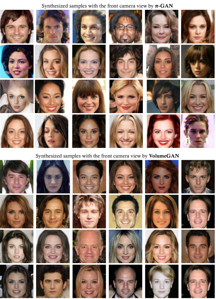
Figure 1: More Synthesized results with the front camera view by $\pi$-GAN [1] and our VolumeGAN, where the faces proposed by VolumeGAN are more consistent with the given view, suggesting a better 3D controllability.

References

- [1] Eric R Chan, Marco Monteiro, Petr Kellnhofer, Jiajun Wu, and Gordon Wetzstein. pi-gan: Periodic implicit generative adversarial networks for 3d-aware image synthesis. In IEEE Conf. Comput. Vis. Pattern Recog., 2021.
- [2] Thu Nguyen-Phuoc, Chuan Li, Lucas Theis, Christian Richardt, and Yong-Liang Yang. Hologan: Unsupervised learning of 3d representations from natural images. In ICCV, 2019.
- [3] Michael Niemeyer and Andreas Geiger. Giraffe: Representing scenes as compositional generative neural feature fields. In IEEE Conf. Comput. Vis. Pattern Recog., 2021.
- [4] Ethan Perez, Florian Strub, Harm De Vries, Vincent Dumoulin, and Aaron Courville. Film: Visual reasoning with a general conditioning layer. In AAAI, 2018.
- [5] Katja Schwarz, Yiyi Liao, Michael Niemeyer, and Andreas Geiger. Graf: Generative radiance fields for 3d-aware image synthesis. In Adv. Neural Inform. Process. Syst., 2020.
- [6] Vincent Sitzmann, Julien Martel, Alexander Bergman, David Lindell, and Gordon Wetzstein. Implicit neural representations with periodic activation functions. NIPS, 2020.