Scattering Amplitudes, the Tail Effect, and Conservative Binary Dynamics at ${\cal O}(G^{4})$

Abstract

We complete the calculation of conservative two-body scattering dynamics at fourth post-Minkowskian order, i.e. ${\cal O}(G^{4})$ and all orders in velocity, including radiative contributions corresponding to the tail effect in general relativity. As in previous calculations, we harness powerful tools from the modern scattering amplitudes program including generalized unitarity, the double copy, and advanced multiloop integration methods, in combination with effective field theory. The classical amplitude involves complete elliptic integrals, and polylogarithms with up to transcendental weight two. Using the amplitude-action relation, we obtain the radial action directly from the amplitude, and match the known overlapping terms in the post-Newtonian expansion.

Introduction. Gravitational-wave science has opened up a new direction in theoretical high energy physics: leveraging advances in quantum field theory (QFT) to develop new tools for the state-of-the-art prediction of gravitational-wave signals. This era of ever-increasing precision holds the promise of new and unexpected discoveries in astronomy, cosmology, and particle physics LIGO ; NewDetectors , but hinges crucially on complementary advances in our theoretical modeling of binary sources. In recent years, a new program for understanding the nature of gravitational-wave sources based on tools from scattering amplitudes and effective field theory (EFT) has emerged.

The central rationale of the new QFT-based approach is to derive classical binary dynamics from scattering amplitudes in order to take full advantage of relativity, on-shell methods GeneralizedUnitarity , double-copy relations between gauge and gravity theories KLT ; BCJ , advanced multiloop integration IBP ; DEs ; FIRE ; PRZ , and EFT methods Weinberg:1978kz ; NeillandRothstein ; 2PM . These are the engines that drive modern scattering amplitude calculations in particle theory, but had not been fully integrated together and applied for gravitational-wave signals. This program is rooted in the well-known connection of scattering amplitudes to general relativity corrections to Newton’s potential ScatteringToGrav ; RecentAmpToPotential ; NeillandRothstein , and in the pioneering application of EFT to gravitational-wave physics NRGR . It also complements traditional approaches to binary dynamics such as effective one-body EOB , numerical relativity NR , gravitational self-force self_force ; SelfForceReview , and perturbation theory in the post-Newtonian (PN) PN ; 4PNDJS ; 4PNrest ; Bini:2017wfr ; Blumlein6PN , post-Minkowskian (PM) PM ; PMModernList , and non-relativistic general relativity NRGR ; NRGRrecent frameworks.

Scattering amplitude methods for determining binary dynamics from potential gravitons have been used in Refs. 3PM ; 3PMLong ; 4PMPotential to derive state-of-the-art results, which have been confirmed in multiple studies 6PNBlumlein ; 3PMFeynman ; 3PMworldline ; Bini:2020wpo ; Bini:2020nsb ; Dlapa:2021npj . Until now, radiative effects at all orders in velocity have only been considered at ${\cal O}(G^{3})$, where radiation reaction is purely dissipative and can be cleanly separated and computed KMOC ; UltraRelativisticLimit ; HPRZ ; OtherVeneziano ; HPRZ2 ; BDGcons . Radiative effects have new features at ${\cal O}(G^{4})$, such as conservative contributions arising from two radiation gravitons known as the tail effect TailEffect ; NewTailPapers , as well as nonlinear dissipative effects that mix with time-reversal invariant conservative effects BDGcons . In this Letter we extend amplitude methods to include all conservative contributions to two-body scattering dynamics.

Our complete result for the conservative contributions ultimately follows from the same condition used to determine the potential graviton contributions 3PM ; 3PMLong ; 4PMPotential . Thus, while extracting conservative dynamics in the presence of radiation involves additional diagrams and expanding integrals in a new region, it is conceptually no more difficult. Remarkably, at this order in the $G$ expansion, the result obtained with the standard Feynman ${\rm i}\varepsilon$ prescription is consistent with using Wheeler-Feynman time-symmetric graviton propagators, as advocated in Ref. BDGcons .

The classical amplitude presented in Eq. (3) below includes both the radiative contributions found here and the potential contributions from our previous work 4PMPotential . It determines the complete conservative two-body scattering dynamics at ${\cal O}(G^{4})$ and all orders in velocity. Using the amplitude-action relation introduced in Ref. 4PMPotential (see also Refs. RadialOthers ), we determine the radial action in Eq. (5). As usual, overlapping results from different techniques help guide new calculations and provide explicit benchmarks. Our result for the ${\cal O}(G^{4})$ scattering angle agrees with the sixth PN order result of Ref. BDGcons . We also agree with the fifth PN order result of Ref. Blumlein:2021txe up to a single term of higher order in the self-force expansion, whose origin requires further study.

Conservative Radiative Effects. The four-point amplitude ${\cal M}$ of gravitationally-interacting minimally-coupled massive scalars encodes conservative two-body scattering dynamics in the classical limit. To compute the amplitude, we follow textbook QFT rules, such as the use of the Feynman $\mathrm{i}\varepsilon$-prescription for all propagators. Our task is then to impose conditions that project out quantum and dissipative parts, leaving only the contributions to the full classical conservative dynamics.

We take the classical limit of ${\cal M}$ by expanding in large angular momentum $J\gg\hbar$ 2PM ; 3PM ; 3PMLong . This amounts to rescaling the momentum transfer $q$ and all graviton loop momenta $\ell$ as $q,\ell\to\lambda q,\lambda\ell$ and then expanding in small $\lambda$. The classical expansion is thus equivalent to an expansion in the soft region, defined by the loop-momentum scaling $\ell=(\omega,\bm{\ell})\sim(\lambda,\lambda)$.

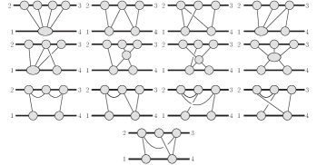
Figure 1: Complete set of generalized unitarity cuts for conservative contributions at $O(G^{4})$. Exposed lines are on-shell. Thick lines represent massive scalars and thin lines are gravitons. The first eight cuts contain both (ppp) and (prr) contributions, while the last five, which have gravitons starting and ending on the same matter line, have no (ppp) contributions.

To define conservative dynamics in the presence of radiative effects, we evaluate integrals by picking up positive-energy residues of matter propagators 2PM ; 3PM ; 3PMLong ; 4PMPotential . A key implication of this is that we only need to consider cuts that have at least one on-shell matter line per loop. This is the same condition that identifies contributions from potential gravitons, and vastly simplifies the analysis. The relevant cuts are shown in Fig. 1.

Notably, the setup described above assumes the standard Feynman $\mathrm{i}\varepsilon$-prescription for graviton propagators, but is consistent with using a principal-value (PV) prescription corresponding to a time-symmetric propagator PVPrescription ; DamourPV ,

$$G^{\mathrm{PV}}(k)=\mathcal{P}\frac{1}{k^{2}}\,,$$ (1)

where $\mathcal{P}$ denotes the principal value. That is, for the part of the three-loop amplitude determined by these cuts, the PV prescription gives the same result as using the standard Feynman $\mathrm{i}\varepsilon$-prescription for graviton propagators and then taking the real part of the final classical amplitude. Note that the prescription in (1) requires some care when applied to multiple propagators PVSubtlety .

We use the method of regions Beneke:1997zp , separating the soft region into the potential (p) and radiation (r) subregions defined by the following scalings of the loop momenta $\ell$:

$$\text{(p)}:\ell\sim(v\lambda,\lambda)\,,\quad\text{(r)}:\ell\sim(v\lambda,v\lambda)\,.$$ (2)

Here $v$ denotes the typical velocity of the binary constituents, corresponding to the small velocity that defines the PN expansion. The classical contribution to any integral is obtained by expanding the three loop momenta in these regions: $(\ell_{1}\ell_{2}\ell_{3})\sim$ (ppp), (ppr), (prr), and (rrr). Of these combinations, only (ppp) and (prr) are relevant for conservative dynamics since (rrr) leads to scaleless integrals and (ppr) yields odd-in-$v$ contributions, which capture dissipative effects and are thus removed by the PV-prescription (1). Effects from the square of radiation-reaction, which are dissipative but even-in-$v$, are also removed by the PV-prescription. The contributions from the potential region (ppp) have been computed in our previous work 4PMPotential and confirmed in Refs. Blumlein6PN ; Dlapa:2021npj . In this Letter we focus on the remaining conservative contribution, originating from the (prr) region.

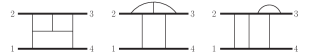
Figure 2: Sample diagrams at ${\cal O}(G^{4})$. From left to right: a diagram with both (ppp) and (prr) contributions, a diagram with only (prr) contributions, a diagram containing iteration terms that cancel in the total amplitude.

Constructing the Integrand. As in our previous work 3PM ; 3PMLong ; 4PMPotential , we use generalized unitarity and the $D$-dimensional tree-level BCJ double copy to construct an integrand that captures the complete conservative dynamics. We sew together tree-level amplitudes in such a way that terms in the physical state projectors that depend on light-cone reference momenta drop out automatically Kosmopoulos:2020pcd . The relevant radiative contributions come from generalized unitarity cuts containing one Compton tree amplitude, and two connected five-point tree amplitudes, each with one cut graviton line to separate the two matter particles. The subset of these cuts containing gravitons beginning and ending on the same matter line contribute only to (prr), while the rest contribute to both (ppp) and (prr). As before, graphs with graviton bubbles and matter contact interactions do not contribute. The relevant cuts including both radiative and potential contributions are shown in Fig. 1; others are obtained by relabeling the external momenta.

The resulting integrand is organized in terms of 93 distinct cubic-vertex Feynman-like diagrams, of which three are shown in Fig. 2. Upon expansion in the soft region, the propagators of certain diagrams, such as the second and third in Fig. 2, become linearly dependent. This is a feature observed in the method of regions Beneke:1997zp , and described in Ref. HPRZ2 in the context of the soft expansion employed here. The products of independent propagators resulting from partial fraction decomposition can be assigned, upon multiplication and division by suitable propagators, to 51 distinct graphs with only cubic vertices.

In contrast to calculations at lower orders, the integrand at ${\cal O}(G^{4})$ depends on whether we use four- or $D$-dimensional states on cut lines. This is presumably related to subtleties associated with non-conventional forms of dimensional regularization (see e.g. Ref. DimReductionSubtlety ). To avoid such issues we use conventional dimensional regularization where all states and momenta are uniformly continued to $D=4-2\epsilon$ dimensions.

Evaluating the Integrals. The resulting integrals are reduced to a basis of master integrals using integration-by-parts (IBP) identities IBP and graph symmetries. An important insight is that IBP relations are agnostic to the choice of graviton propagator prescriptions. This allows us to make use of automated tools such as FIRE6 FIRE and KIRA KIRA , which are usually applied to cases with Feynman propagators, to reduce integrals with the prescription (1).

We evaluate the master integrals using the method of differential equations DEs ; PRZ with boundary conditions determined either in the (ppp) or (prr) region, and using the PV prescription (1). Since they are disjoint, they can be treated separately, and the complete system of linear differential equations splits into two partly-overlapping sectors each with non-vanishing boundary conditions in one of the two regions. The overlap is given by integrals with non-trivial boundary conditions in both regions, which are those captured by the first eight cuts in Fig. 1.

The system of differential equations was solved in the (ppp) region in Ref. 4PMPotential in terms of classical polylogarithms up to weight three and complete elliptic integrals. The system for the integrals in the (prr) region can be brought to canonical form Henn , which allows us to evaluate the integrals to arbitrary order in the dimensional regulator $\epsilon=(4-D)/2$. The canonical form also implies that elliptic integrals are absent in the (prr) region. We have evaluated the integrals up to transcendental weight three. Note that due to the requirement of one on-shell matter line per loop, each of the $L$ loops introduces a factor of $\pi$, and therefore the maximal weight is $L$ instead of $2L$ for a general $L$-loop amplitude Arkani-Hamed:2010pyv . We have also verified that our integration method is consistent with the nonrelativistic integration approach 2PM ; 3PM ; 3PMLong .

Amplitude. The final result for the ${\cal O}(G^{4})$ conservative scattering amplitude in the classical limit including all contributions is

$${\cal M}_{4}^{\rm cons} =G^{4}M^{7}\nu^{2}|\bm{q}|\pi^{2}\left[{\cal M}_{4}^{\rm p}+\nu\left(4{\cal M}_{4}^{\rm t}\log\left(\tfrac{p_{\infty}}{2}\right)+{\cal M}_{4}^{\pi^{2}}+{\cal M}_{4}^{\rm rem}\right)\right]+\int_{\bm{\ell}}\frac{\tilde{I}_{r,1}^{4}}{Z_{1}Z_{2}Z_{3}}+\int_{\bm{\ell}}\frac{\tilde{I}_{r,1}^{2}\tilde{I}_{r,2}}{Z_{1}Z_{2}}+\int_{\bm{\ell}}\frac{\tilde{I}_{r,1}\tilde{I}_{r,3}}{Z_{1}}+\int_{\bm{\ell}}\frac{\tilde{I}_{r,2}^{2}}{Z_{1}}\,,$$

$${\cal M}_{4}^{\rm p} =-\frac{35\left(1-18\sigma^{2}+33\sigma^{4}\right)}{8\left(\sigma^{2}-1\right)}\,,$$

$${\cal M}_{4}^{\rm t} =r_{1}+r_{2}\log\left(\tfrac{\sigma+1}{2}\right)+r_{3}\frac{{\rm arccosh}(\sigma)}{\sqrt{\sigma^{2}-1}}\,,$$ (3)

$${\cal M}_{4}^{\pi^{2}} =r_{4}\pi^{2}+r_{5}\,{\rm K}\big{(}\tfrac{\sigma-1}{\sigma+1}\big{)}{\rm E}\big{(}\tfrac{\sigma-1}{\sigma+1}\big{)}+r_{6}\,{\rm K}^{2}\big{(}\tfrac{\sigma-1}{\sigma+1}\big{)}+r_{7}\,{\rm E}^{2}\big{(}\tfrac{\sigma-1}{\sigma+1}\big{)}\,,$$

$${\cal M}_{4}^{\rm rem} =r_{8}+r_{9}\log\left(\tfrac{\sigma+1}{2}\right)+r_{10}\tfrac{{\rm arccosh}(\sigma)}{\sqrt{\sigma^{2}-1}}+r_{11}\log(\sigma)+r_{12}\log^{2}\left(\tfrac{\sigma+1}{2}\right)+r_{13}\tfrac{\operatorname{arccosh}(\sigma)}{\sqrt{\sigma^{2}-1}}\log\left(\tfrac{\sigma+1}{2}\right)+r_{14}\,\tfrac{{\rm arccosh}^{2}(\sigma)}{\sigma^{2}-1}$$

$$\quad+r_{15}\,\text{Li}_{2}\left(\tfrac{1-\sigma}{2}\right)+r_{16}\,\text{Li}_{2}\big{(}\tfrac{1-\sigma}{1+\sigma}\big{)}+r_{17}\,\tfrac{1}{\sqrt{\sigma^{2}-1}}\left[\text{Li}_{2}\left(-\sqrt{\tfrac{\sigma-1}{\sigma+1}}\right)-\text{Li}_{2}\left(\sqrt{\tfrac{\sigma-1}{\sigma+1}}\right)\right]\,.$$

This result is for the scattering of two scalars with incoming four-momenta $p_{1}$ and $p_{2}$ and masses $m_{1}$ and $m_{2}$. Here $\bm{q}$ is the three-momentum transfer in the center of mass (COM) frame, $M=m_{1}+m_{2}$ is the total mass, $\nu=m_{1}m_{2}/M^{2}$ is the symmetric mass ratio, $\sigma=p_{1}\cdot p_{2}/m_{1}m_{2}$ in the mostly minus signature, and $p_{\infty}=\sqrt{\sigma^{2}-1}$. For later convenience, we also introduce the three-momentum $\bm{p}_{1}=-\bm{p}_{2}=\bm{p}$ in the COM frame, individual energies $E_{i}=\sqrt{\bm{p}^{2}+m_{i}^{2}}$, the total energy $E=E_{1}+E_{2}$, and the symmetric energy ratio $\xi=E_{1}E_{2}/E^{2}$.

The contribution in the probe limit is given by ${\cal M}_{4}^{\rm p}$, while the ${\cal O}(\nu)$ contribution, i.e. first order in the self-force expansion, consists of the logarithmic tail coefficient ${\cal M}_{4}^{\rm t}$, the potential $\pi^{2}$ contribution ${\cal M}_{4}^{\pi^{2}}$, and the remainder ${\cal M}_{4}^{\rm rem}$.

Note that the basis of transcendental functions has been slightly rearranged with respect to Ref. 4PMPotential , and that the rational coefficients, given in Table 1, have simplified upon combining the (ppp) and (prr) contributions. This exposes additional structures; for example the coefficient of $\operatorname{arccosh}^{2}\sigma$ is closely related to that of $\operatorname{arccosh}\sigma$ in $\mathcal{M}_{4}^{\mathrm{t}}$, suggesting that this expression exponentiates. Furthermore, the coefficients of the weight two functions are expressible in terms of the polynomial functions $g_{1},g_{2},g_{3},$ and $g_{4}$. Note that the function $g_{3}$ is related to the leading contribution of the electric Weyl squared tidal operator to two-body scattering DamourTidal .

The remaining integrals in Eq. (3) are contributions from iteration of lower order amplitudes. At ${\cal O}(G^{4})$, these arise only from the (ppp) region, and are thus the same as in our previous work 4PMPotential . Iteration terms in (prr), such as from the last diagram in Fig. 2, cancel in the final amplitude. Similarly, terms of second order in the self-force expansion as well as terms of transcendental weight three appear in intermediate steps but cancel nontrivially in the final amplitude. Note also that the PV prescription eliminates the imaginary part of the amplitude, which is proportional to $\mathcal{M}_{4}^{\mathrm{t}}$.

$$r_{1} =\frac{1151-3336\sigma+3148\sigma^{2}-912\sigma^{3}+339\sigma^{4}-552\sigma^{5}+210\sigma^{6}}{12(\sigma^{2}-1)}$$ $$r_{2} =4g_{1}-2g_{2}-\frac{1}{2}g_{3}$$ $$r_{3} =\frac{\sigma\left(-3+2\sigma^{2}\right)}{4(\sigma^{2}-1)}g_{3}$$ $$r_{4} =-\frac{16}{3}g_{1}+\frac{4}{3}g_{2}-\frac{1}{3}g_{4}$$ $$r_{5} =-\frac{1183+2929\sigma+2660\sigma^{2}+1200\sigma^{3}}{2(\sigma^{2}-1)}$$ $$r_{6} =\frac{834+2095\sigma+1200\sigma^{2}}{2(\sigma^{2}-1)}$$ $$r_{7} =\frac{7\left(169+380\sigma^{2}\right)}{4(\sigma-1)}$$ $$r_{8} =\frac{1}{72(\sigma^{2}-1)^{2}\sigma^{7}}\left(3600\sigma^{16}+4320\sigma^{15}-35360\sigma^{14}+33249\sigma^{13}\right.$$ $$\quad\left.\hbox{}+27952\sigma^{12}-25145\sigma^{11}-15056\sigma^{10}-32177\sigma^{9}+64424\sigma^{8}\right.$$ $$\quad\left.\hbox{}-38135\sigma^{7}+13349\sigma^{6}-1471\sigma^{4}+207\sigma^{2}-45\right)$$ $$r_{9} =-\frac{2\left(75\sigma^{7}-416\sigma^{5}-612\sigma^{4}-739\sigma^{3}-136\sigma^{2}-2520\sigma-152\right)}{3(\sigma^{2}-1)}$$ $$r_{10} =-\frac{\sigma(-3+2\sigma^{2})}{(\sigma^{2}-1)}2r_{1}+28\sigma^{2}(-3+2\sigma^{2})$$ $$r_{11} =\frac{4\sigma}{3(\sigma^{2}-1)}\left(-852-283\sigma^{2}-140\sigma^{4}+75\sigma^{6}\right)$$ $$r_{12} =6g_{2}+g_{3}-\frac{1}{2}g_{4}$$ $$r_{13} =-8\frac{\sigma(-3+2\sigma^{2})}{\sigma^{2}-1}g_{1}$$ $$r_{14} =-\frac{\sigma^{2}(-3+2\sigma^{2})^{2}}{4(\sigma^{2}-1)^{2}}g_{3}$$ $$r_{15} =-16g_{1}-4g_{2}-g_{4}$$ $$r_{16} =-2g_{4}$$ $$r_{17} =-\frac{\sigma(-3+2\sigma^{2})}{\sigma^{2}-1}(8g_{1}-4g_{2})$$ $$g_{1} =2+15\sigma^{2}$$ $$g_{2} =19\sigma+15\sigma^{3}$$ $$g_{3} =11-30\sigma^{2}+35\sigma^{4}$$ $$g_{4} =-20-111\sigma^{2}-30\sigma^{4}+25\sigma^{6}$$

Table 1: Functions specifying the amplitude in Eq. (3).

As for the ${\cal O}(G^{3})$ case, the result in Eq. (3) does not smoothly match onto the massless case. Taking the high energy limit $|\bm{p}|\to\infty$, we find a leading power discontinuity in the classical part of the amplitude

$${\cal M}_{4}^{\rm cons}={560\pi^{2}(2-(2\ln 2+1)^{2})(G{\bm{p}}^{2})^{4}|\bm{q}|\over M\nu}+\dots,$$ (4)

where the ellipses denote terms subleading in large $|\bm{p}|$. It would be interesting to study whether this mass singularity cancels with dissipative effect as it does at $\mathcal{O}(G^{3})$ UltraRelativisticLimit .

Radial Action for Hyperbolic Orbits. Given the amplitude-action relation 4PMPotential , it is straightforward to derive the radial action for hyperbolic orbits from Eq. (3) via an inverse two-dimensional Fourier-transform. We find the radial action in the COM frame

$$I^{\rm hyp}_{r,4} =-\frac{G^{4}M^{7}\nu^{2}\pi{\bm{p}}^{2}}{8EJ^{3}}$$ (5)

$$\times\left[{\cal M}_{4}^{\rm p}+\nu\left(4{\cal M}_{4}^{\rm t}\log\left(\tfrac{p_{\infty}}{2}\right)+{\cal M}_{4}^{\pi^{2}}+{\cal M}_{4}^{\rm rem}\right)\right]\,,$$

which inherits the simple mass dependence from the amplitude Bini:2020wpo ; DamourSelfForce . The radial action (5) in Mathematica text format is given in the ancillary file AttachedFile . As an explicit benchmark, let us consider the nonlogarithmic (prr) contributions to the radial action defined in Ref. BDGcons as ${\cal M}_{4}^{\rm radgrav,f}\equiv 14{\cal M}_{4}^{\rm t}+{\cal M}_{4}^{\rm rem,prr}$, with ${\cal M}_{4}^{\rm rem,prr}$ given in the Appendix. Expanding this through ninth PN order, we find

$${\cal M}_{4}^{\rm radgrav,f} ={12044\over 75}p^{2}_{\infty}+{212077\over 3675}p^{4}_{\infty}+{115917979\over 793800}p^{6}_{\infty}$$

$$\quad-{9823091209\over 76839840}p^{8}_{\infty}+{115240251793703\over 1038874636800}p^{10}_{\infty}$$

$$\quad-{411188753665637\over 4155498547200}p^{12}_{\infty}+\cdots\,,$$ (6)

whose first three terms match the sixth PN order result in Eq. (6.20) of Ref. BDGcons .

The scattering angle is given by $\chi_{4}=-\partial I_{r,4}^{\rm hyp}/\partial J$. After expanding in velocity, our result agrees with the sixth PN order result in Eq. (6.17) of Ref. BDGcons . In particular, we find that terms of second order in the self-force expansion are absent, consistent with Ref. BDGcons . On the other hand, the result of Ref. Blumlein:2021txe does contain such a term (see Eq. (69) therein). Aside from the angle, another gauge-invariant observable is the time-delay for hyperbolic orbits given by $\partial I_{r,4}^{\rm hyp}/\partial E$.

Local Hamiltonian for Hyperbolic Orbits. The presence of radiation leads to nonlocal-in-time contributions to classical dynamics TailEffect . Following previous analyses 2PM ; 3PMLong ; 4PMPotential , a two-body Hamiltonian can be derived from the radial action in Eq. (5). This Hamiltonian is effectively local and captures the nonlocal-in-time Hamiltonian evaluated on the relevant orbits. For completeness, the effective local Hamiltonian valid for hyperbolic orbits is:

$$H^{\rm hyp}=E_{1}+E_{2}+\sum_{n=1}^{\infty}{G^{n}\over r^{n}}c_{n}(\bm{p}^{2})\,,$$ (7)

where $r$ is the distance between the bodies in the COM frame. We have checked that $H^{\rm hyp}$ reproduces the scattering angle. The lower-order coefficients $c_{1}$, $c_{2}$, and $c_{3}$ can be found in Eq. (10) of Ref. 3PM , while $c_{4}=c_{4}^{\rm hyp}$ is

$$c_{4}^{\rm hyp} ={M^{7}\nu^{2}\over 4\xi E^{2}}\left[{\cal M}_{4}^{\rm p}+\nu{}\left(4{\cal M}_{4}^{\rm t}\log\left(\tfrac{p_{\infty}}{2}\right)+{\cal M}_{4}^{\pi^{2}}+{\cal M}_{4}^{\rm rem}\right)\right]+{\cal D}^{3}\left[{E^{3}\xi^{3}\over 3}c_{1}^{4}\right]+{\cal D}^{2}\left[\left(\frac{E^{3}\xi^{3}}{\bm{p}^{2}}+\frac{E\xi{}(3\xi-1)}{2}\right)c_{1}^{4}-2E^{2}\xi^{2}c_{1}^{2}c_{2}\right]$$

$$\quad+\left({\cal D}+{1\over\bm{p}^{2}}\right)\bigg{[}E\xi{}(2c_{1}c_{3}+c_{2}^{2})+\left(\frac{4\xi-1}{4E}+\frac{2E^{3}\xi^{3}}{\bm{p}^{4}}+\frac{E\xi(3\xi-1)}{\bm{p}^{2}}\right)c_{1}^{4}+\left((1-3\xi)-\frac{4E^{2}\xi^{2}}{\bm{p}^{2}}\right)c_{1}^{2}c_{2}\bigg{]}\,,$$ (8)

where ${\cal D}={d\over d\bm{p}^{2}}$ denotes differentiation with respect to $\bm{p}^{2}$. The final explicit result for $c_{4}^{\rm hyp}$ is included in the ancillary file AttachedFile . Again, the label ‘hyp’ emphasizes that $c_{4}^{\rm hyp}$ applies only for hyperbolic orbits. Nonetheless, the potential contributions to ${\cal M}_{4}^{\pi^{2}}$ and the coefficient of logarithm, ${\cal M}_{4}^{\rm t}$, are local and should analytically continue between bound and unbound orbits Bini:2017wfr ; Cho:2021arx .

Conclusions. We extended amplitudes methods to include the full conservative contributions in classical two-body scattering at ${\cal O}(G^{4})$. Compared to our previous work on pure potential contributions 4PMPotential , this involves additional unitarity cuts and altered boundary conditions for the differential equations that determine the master integrals. An important next step will be to understand how to convert results for scattering in the presence of conservative radiative effects to ones for the bound-state problem Bini:2017wfr ; Cho:2021arx . It will also be interesting to study the impact of our results on waveform generation BuonannoEnergetics .

We expect that a setup similar to the one used at $\mathcal{O}(G^{3})$ HPRZ2 based on the formalism of Ref. KMOC can be used to derive the dissipative radiation reaction contributions to the scattering angle at $\mathcal{O}(G^{4})$. Perhaps the most exciting development is that we encountered no conceptual or technical obstructions to pushing PM scattering calculations to increasingly high orders and extracting from them the complete conservative scattering dynamics of two-body systems.

Acknowledgments. We thank Johannes Blümlein, Martin Bojowald, Alessandra Buonanno, Clifford Cheung, Thibault Damour, Enrico Herrmann, Mohammed Khalil, David Kosower, Andrés Luna, Andreas Maier, Philipp Maierhöfer, Aneesh Manohar, Peter Marquard, Rafael Porto, Ira Rothstein, Jan Steinhoff, Johann Usovitsch, and Justin Vines for helpful discussions. Z.B. is supported by the U.S. Department of Energy (DOE) under award number DE-SC0009937. J.P.-M. is supported by the U.S. Department of Energy (DOE) under award number DE-SC0011632. R.R. is supported by the U.S. Department of Energy (DOE) under award number DE-SC00019066. C.-H.S. is supported by the U.S. Department of Energy (DOE) under award number DE-SC0009919. M.Z.’s work is supported by the U.K. Royal Society through Grant URF\R1\20109. We also are grateful to the Mani L. Bhaumik Institute for Theoretical Physics for support.

Appendix A Amplitude in different regions.

$$r^{\rm ppp}_{8} =\vphantom{\frac{1}{2}}\frac{1}{144\bigl{(}\sigma^{2}-1)^{2}\sigma^{7}}(-45+207\sigma^{2}-1471\sigma^{4}+13349\sigma^{6}$$ $$\quad-37566\sigma^{7}+104753\sigma^{8}-12312\sigma^{9}-102759\sigma^{10}-105498\sigma^{11}$$ $$\quad+134745\sigma^{12}+83844\sigma^{13}-101979\sigma^{14}+13644\sigma^{15}+10800\sigma^{16}\bigr{)}$$ $$r^{\rm ppp}_{9} =\vphantom{\frac{1}{2}}\frac{1}{4(\sigma^{2}-1)}\bigl{(}1759-4768\sigma+3407\sigma^{2}-1316\sigma^{3}+957\sigma^{4}$$ $$\quad-672\sigma^{5}+341\sigma^{6}+100\sigma^{7}\bigr{)}$$ $$r^{\rm ppp}_{10} =\vphantom{\frac{1}{2}}\frac{1}{24(\sigma^{2}-1)^{2}}\bigl{(}1237+7959\sigma-25183\sigma^{2}+12915\sigma^{3}+18102\sigma^{4}$$ $$\quad-12105\sigma^{5}-9572\sigma^{6}+2973\sigma^{7}+5816\sigma^{8}-2046\sigma^{9}\bigr{)}$$ $$r^{\rm ppp}_{11} =\vphantom{\frac{1}{2}}\frac{2\sigma\left(-852-283\sigma^{2}-140\sigma^{4}+75\sigma^{6}\right)}{3(\sigma^{2}-1)}$$ $$r^{\rm ppp}_{12} =\vphantom{\frac{1}{2}}4g_{1}-7g_{2}-\frac{3}{4}g_{4}$$ $$r^{\rm ppp}_{13} =\vphantom{\frac{1}{2}}0$$ $$r^{\rm ppp}_{14} =\vphantom{\frac{1}{2}}-\frac{\sigma^{2}\left(-3+2\sigma^{2}\right)^{2}}{8(\sigma^{2}-1)^{2}}g_{3}+2(\sigma^{2}-1)g_{2}$$ $$r^{\rm ppp}_{15} =\vphantom{\frac{1}{2}}24g_{1}-14g_{2}+2g_{3}-\frac{3}{2}g_{4}$$ $$r^{\rm ppp}_{16} =\vphantom{\frac{1}{2}}-g_{4}$$ $$r^{\rm ppp}_{17} =\vphantom{\frac{1}{2}}-\frac{\sigma(-3+2\sigma^{2})}{\sigma^{2}-1}(8g_{1}-4g_{2})$$ $$r^{\rm ppp}_{18} =\vphantom{\frac{1}{2}}\frac{\sigma\left(-3+2\sigma^{2}\right)}{2(\sigma^{2}-1)}\,g_{3}$$

Table 2: Functions specifying the amplitude in the ppp region.

$$r^{\rm prr}_{8} =\vphantom{\frac{1}{2}}\frac{1}{144\sigma^{7}\left(\sigma^{2}-1\right)^{2}}(-45+207\sigma^{2}-1471\sigma^{4}+13349\sigma^{6}$$ $$\quad-38704\sigma^{7}+24095\sigma^{8}-52042\sigma^{9}+72647\sigma^{10}+55208\sigma^{11}$$ $$\quad-78841\sigma^{12}-17346\sigma^{13}+31259\sigma^{14}-5004\sigma^{15}-3600\sigma^{16})$$ $$r^{\rm prr}_{9} =\vphantom{\frac{1}{2}}\frac{1}{12\left(\sigma^{2}-1\right)}(-4061+34464\sigma-9133\sigma^{2}+9860\sigma^{3}+2025\sigma^{4}$$ $$\quad+5344\sigma^{5}-1023\sigma^{6}-900\sigma^{7})$$ $$r^{\rm prr}_{10} =\vphantom{\frac{1}{2}}\frac{1}{24(\sigma^{2}-1)^{2}}(-1237+5853\sigma-16865\sigma^{2}+15653\sigma^{3}+3018\sigma^{4}$$ $$\quad-9011\sigma^{5}+5540\sigma^{6}-3165\sigma^{7}-56\sigma^{8}+366\sigma^{9})$$ $$r^{\rm prr}_{11} =\vphantom{\frac{1}{2}}\frac{2\sigma\left(-852-283\sigma^{2}-140\sigma^{4}+75\sigma^{6}\right)}{3(\sigma^{2}-1)}$$ $$r^{\rm prr}_{12} =\vphantom{\frac{1}{2}}-4g_{1}+13g_{2}+g_{3}+\frac{1}{4}g_{4}$$ $$r^{\rm prr}_{13} =\vphantom{\frac{1}{2}}-8\frac{\sigma\left(-3+2\sigma^{2}\right)}{(\sigma^{2}-1)}g_{1}$$ $$r^{\rm prr}_{14} =\vphantom{\frac{1}{2}}-\frac{\sigma^{2}\left(-3+2\sigma^{2}\right)^{2}}{8(\sigma^{2}-1)^{2}}g_{3}-2(\sigma^{2}-1)g_{2}$$ $$r^{\rm prr}_{15} =\vphantom{\frac{1}{2}}-40g_{1}+10g_{2}-2g_{3}+\frac{1}{2}g_{4}$$ $$r^{\rm prr}_{16} =\vphantom{\frac{1}{2}}-g_{4}$$ $$r^{\rm prr}_{17} =\vphantom{\frac{1}{2}}0$$ $$r^{\rm prr}_{18} =\vphantom{\frac{1}{2}}-\frac{\sigma\left(-3+2\sigma^{2}\right)}{2(\sigma^{2}-1)}g_{3}$$

Table 3: Functions specifying the amplitude in the prr region.

In this appendix we present the scattering amplitudes in the (ppp) and (prr) regions separately. The contribution from the (ppp) region already appeared in Ref. 4PMPotential and is given by

$${\cal M}_{4}^{\mathrm{ppp}}(\bm{q})=G^{4}M^{7}\nu^{2}|\bm{q}|\pi^{2}2^{2\epsilon}\left(\frac{\bm{q}^{2}}{\tilde{\mu}^{2}}\right)^{-3\epsilon}$$

$$\qquad\times\left[{\cal M}_{4}^{\rm p}+\nu\left(\frac{{\cal M}_{4}^{\rm t}}{\epsilon}+{\cal M}_{4}^{\pi^{2}}+{\cal M}_{4}^{\rm rem,ppp}\right)\right]$$ (9)

$$\qquad+\int_{\bm{\ell}}\frac{\tilde{I}_{r,1}^{4}}{Z_{1}Z_{2}Z_{3}}+\int_{\bm{\ell}}\frac{\tilde{I}_{r,1}^{2}\tilde{I}_{r,2}}{Z_{1}Z_{2}}+\int_{\bm{\ell}}\frac{\tilde{I}_{r,1}\tilde{I}_{r,3}}{Z_{1}}+\int_{\bm{\ell}}\frac{\tilde{I}_{r,2}^{2}}{Z_{1}}\,,$$

where ${\cal M}_{4}^{\rm p}$, ${\cal M}_{4}^{\pi^{2}}$, ${\cal M}_{4}^{\rm t}$ and the iteration integrals are as given in the main text in Eq. (3), and ${\cal M}_{4}^{\pi^{2}}+{\cal M}_{4}^{\rm rem,ppp}={\cal M}_{4}^{\rm f}$ defined in Eq. (6) of Ref. 4PMPotential . The new result from the (prr) region is

$${\cal M}_{4}^{\mathrm{prr}}(\bm{q}) =G^{4}M^{7}\nu^{3}|\bm{q}|\pi^{2}2^{6\epsilon}p_{\infty}^{-4\epsilon}\left(\frac{\bm{q}^{2}}{\tilde{\mu}^{2}}\right)^{-3\epsilon}$$

$$\hskip 56.9055pt\times\left(-\frac{{\cal M}_{4}^{\rm t}}{\epsilon}+{\cal M}_{4}^{\rm rem,prr}\right).$$ (10)

The remainder functions in both regions are given by

$${\cal M}_{4}^{\rm rem,x}=r^{x}_{8}+r^{x}_{9}\log\big{(}\tfrac{\sigma+1}{2}\big{)}+r^{x}_{10}\frac{{\rm arccosh}(\sigma)}{\sqrt{\sigma^{2}-1}}+r^{x}_{11}\log(\sigma)$$

$$\quad+r^{x}_{12}\log^{2}\left(\tfrac{\sigma+1}{2}\right)+r^{x}_{13}\frac{\operatorname{arccosh}(\sigma)}{\sqrt{\sigma^{2}-1}}\log\left(\tfrac{\sigma+1}{2}\right)$$

$$\quad+r^{x}_{14}\,\frac{{\rm arccosh}^{2}(\sigma)}{\sigma^{2}-1}+r^{x}_{15}\text{Li}_{2}\left(\tfrac{1-\sigma}{2}\right)+r^{x}_{16}\text{Li}_{2}\big{(}\tfrac{1-\sigma}{1+\sigma}\big{)}$$

$$\quad+r^{x}_{17}\frac{1}{\sqrt{\sigma^{2}-1}}\left[\text{Li}_{2}\left(-\sqrt{\tfrac{\sigma-1}{\sigma+1}}\right)-\text{Li}_{2}\left(\sqrt{\tfrac{\sigma-1}{\sigma+1}}\right)\right]$$

$$\quad+r^{x}_{18}\frac{1}{\sqrt{\sigma^{2}-1}}F(\sigma){}\,,$$ (11)

where the relevant coefficients $r^{x}_{i}$ in each region, $x={\rm ppp}$, ${\rm prr}$, are given in Tables 3 and 3 respectively in terms of the polynomials $g_{i}$ in Table  1. The transcendental function $F(\sigma)$ in Eq. (11) above is defined as

$$F(\sigma) =\text{Li}_{2}\!\left(\!1\!-\!\sigma\!-\!\sqrt{\sigma^{2}-1}\right)\!-\!\text{Li}_{2}\!\left(\!1\!-\!\sigma\!+\!\sqrt{\sigma^{2}-1}\right)$$

$$+3\text{Li}_{2}\!\left(\!\sqrt{\tfrac{\sigma-1}{\sigma+1}}\right)\!-\!3\text{Li}_{2}\!\left(\!-\sqrt{\tfrac{\sigma-1}{\sigma+1}}\right)$$

$$+2\log\left(\tfrac{\sigma+1}{2}\right){\rm arccosh}(\sigma)\,,$$ (12)

and its coefficients cancel when both regions are combined.

References

- (1) B. P. Abbott et al. [LIGO Scientific and Virgo Collaborations], Phys. Rev. Lett. 116, no. 6, 061102 (2016) [arXiv:1602.03837 [gr-qc]]; B. P. Abbott et al. [LIGO Scientific and Virgo Collaborations], Phys. Rev. Lett. 119, no. 16, 161101 (2017) [arXiv:1710.05832 [gr-qc]].
- (2) M. Punturo et al., Class. Quant. Grav. 27 (2010) 194002; P. Amaro-Seoane et al. [LISA], [arXiv:1702.00786 [astro-ph.IM]]; D. Reitze et al. Bull. Am. Astron. Soc. 51, 035 [arXiv:1907.04833 [astro-ph.IM]].
- (3) Z. Bern, L. J. Dixon, D. C. Dunbar and D. A. Kosower, Nucl. Phys. B 425, 217 (1994) [hep-ph/9403226]; Z. Bern, L. J. Dixon, D. C. Dunbar and D. A. Kosower, Nucl. Phys. B 435, 59 (1995) [hep-ph/9409265]; Z. Bern and A. G. Morgan, Nucl. Phys. B 467, 479 (1996) [hep-ph/9511336]; Z. Bern, L. J. Dixon and D. A. Kosower, Nucl. Phys. B 513, 3 (1998) [hep-ph/9708239]; R. Britto, F. Cachazo and B. Feng, Nucl. Phys. B 725, 275 (2005) [hep-th/0412103]; Z. Bern, J. J. M. Carrasco, H. Johansson and D. A. Kosower, Phys. Rev. D 76, 125020 (2007) [arXiv:0705.1864 [hep-th]].
- (4) H. Kawai, D. C. Lewellen and S. H. H. Tye, Nucl. Phys. B 269, 1 (1986); Z. Bern, L. J. Dixon, M. Perelstein and J. S. Rozowsky, Nucl. Phys. B 546, 423 (1999) [hep-th/9811140].
- (5) Z. Bern, J. J. M. Carrasco and H. Johansson, Phys. Rev. D 78, 085011 (2008) [arXiv:0805.3993 [hep-ph]]; Z. Bern, J. J. M. Carrasco and H. Johansson, Phys. Rev. Lett. 105, 061602 (2010) [arXiv:1004.0476 [hep-th]]; Z. Bern, J. J. M. Carrasco, W. M. Chen, H. Johansson, R. Roiban and M. Zeng, Phys. Rev. D 96, no.12, 126012 (2017) [arXiv:1708.06807 [hep-th]]; Z. Bern, J. J. Carrasco, W. M. Chen, A. Edison, H. Johansson, J. Parra-Martinez, R. Roiban and M. Zeng, Phys. Rev. D 98, no.8, 086021 (2018) [arXiv:1804.09311 [hep-th]]; Z. Bern, J. J. Carrasco, M. Chiodaroli, H. Johansson and R. Roiban, arXiv:1909.01358 [hep-th].
- (6) K.G. Chetyrkin and F.V. Tkachov, Nucl. Phys. B 192, 159 (1981); S. Laporta, Int. J. Mod. Phys. A 15, 5087-5159 (2000) [arXiv:hep-ph/0102033 [hep-ph]].
- (7) A. V. Kotikov, Phys. Lett. B 254, 158-164 (1991); Z. Bern, L. J. Dixon and D. A. Kosower, Nucl. Phys. B 412, 751-816 (1994) [arXiv:hep-ph/9306240 [hep-ph]]; E. Remiddi, Nuovo Cim. A 110, 1435-1452 (1997) [arXiv:hep-th/9711188 [hep-th]]; T. Gehrmann and E. Remiddi, Nucl. Phys. B 580, 485-518 (2000) [arXiv:hep-ph/9912329 [hep-ph]].
- (8) A. V. Smirnov, JHEP 10, 107 (2008) [arXiv:0807.3243 [hep-ph]]; A. V. Smirnov and F. S. Chuharev, Comput. Phys. Commun. 247 , 106877 (2020) [arXiv:1901.07808 [hep-ph]].
- (9) J. Parra-Martinez, M. S. Ruf and M. Zeng, JHEP 11, 023 (2020) [arXiv:2005.04236 [hep-th]].
- (10) S. Weinberg, Physica A 96, no.1-2, 327-340 (1979)
- (11) D. Neill and I. Z. Rothstein, Nucl. Phys. B 877, 177-189 (2013) [arXiv:1304.7263 [hep-th]].
- (12) C. Cheung, I. Z. Rothstein and M. P. Solon, Phys. Rev. Lett. 121, no.25, 251101 (2018) [arXiv:1808.02489 [hep-th]].
- (13) Y. Iwasaki, Prog. Theor. Phys. 46, 1587 (1971); Y. Iwasaki, Lett. Nuovo Cim. 1S2, 783 (1971) [Lett. Nuovo Cim. 1, 783 (1971)]; S. N. Gupta and S. F. Radford, Phys. Rev. D 19, 1065 (1979).
- (14) J. F. Donoghue, Phys. Rev. D 50, 3874-3888 (1994) [arXiv:gr-qc/9405057 [gr-qc]]; N. E. J. Bjerrum-Bohr, J. F. Donoghue and B. R. Holstein, Phys. Rev. D 67, 084033 (2003) [erratum: Phys. Rev. D 71, 069903 (2005)] [arXiv:hep-th/0211072 [hep-th]]; N. E. J. Bjerrum-Bohr, J. F. Donoghue and P. Vanhove, JHEP 1402, 111 (2014) [arXiv:1309.0804 [hep-th]].
- (15) W. D. Goldberger and I. Z. Rothstein, Phys. Rev. D 73, 104029 (2006) [hep-th/0409156].
- (16) A. Buonanno and T. Damour, Phys. Rev. D 59, 084006 (1999) [gr-qc/9811091]; A. Buonanno and T. Damour, Phys. Rev. D 62, 064015 (2000) [gr-qc/0001013].
- (17) F. Pretorius, Phys. Rev. Lett. 95, 121101 (2005) [gr-qc/0507014]; M. Campanelli, C. O. Lousto, P. Marronetti and Y. Zlochower, Phys. Rev. Lett. 96, 111101 (2006) [gr-qc/0511048]; J. G. Baker, J. Centrella, D. I. Choi, M. Koppitz and J. van Meter, Phys. Rev. Lett. 96, 111102 (2006) [gr-qc/0511103].
- (18) Y. Mino, M. Sasaki and T. Tanaka, Phys. Rev. D 55, 3457 (1997) [gr-qc/9606018]; T. C. Quinn and R. M. Wald, Phys. Rev. D 56, 3381 (1997) [gr-qc/9610053].
- (19) E. Poisson, A. Pound and I. Vega, Living Rev. Rel. 14, 7 (2011) [arXiv:1102.0529 [gr-qc]]; L. Barack and A. Pound, Rept. Prog. Phys. 82, no.1, 016904 (2019) [arXiv:1805.10385 [gr-qc]].
- (20) J. Droste, Proc. Acad. Sci. Amst. 19:447–455 (1916); H. A. Lorentz and J. Droste, Koninklijke Akademie Van Wetenschappen te Amsterdam 26 392, 649 (1917). English translation in “Lorentz Collected papers,” P. Zeeman and A. D. Fokker editors, Vol 5, 330 (1934-1939), The Hague: Nijhof; A. Einstein, L. Infeld and B. Hoffmann, Annals Math. 39, 65 (1938); T. Ohta, H. Okamura, T. Kimura and K. Hiida, Prog. Theor. Phys. 50, 492 (1973); T. Damour and N. Deruelle, Phys. Lett. A 87, 81 (1981); T. Damour, C.R. Acad. Sc. Paris, Série II, 294, pp 1355-1357 (1982); P. Jaranowski and G. Schäfer, Phys. Rev. D 57, 7274 (1998) Erratum: [Phys. Rev. D 63, 029902 (2000)] [gr-qc/9712075]; T. Damour, P. Jaranowski and G. Schäfer, Phys. Rev. D 62, 044024 (2000) [gr-qc/9912092]; L. Blanchet and G. Faye, Phys. Lett. A 271, 58 (2000) [gr-qc/0004009]; L. Blanchet and G. Faye, Phys. Rev. D 63, 062005 (2001) [arXiv:gr-qc/0007051 [gr-qc]]; V. C. de Andrade, L. Blanchet and G. Faye, Class. Quant. Grav. 18, 753-778 (2001) [arXiv:gr-qc/0011063 [gr-qc]]; T. Damour, P. Jaranowski and G. Schäfer, Phys. Lett. B 513, 147 (2001) [gr-qc/0105038]; L. Blanchet and B. R. Iyer, Class. Quant. Grav. 20, 755 (2003) [arXiv:gr-qc/0209089 [gr-qc]]; L. Blanchet, T. Damour and G. Esposito-Farese, Phys. Rev. D 69, 124007 (2004) [arXiv:gr-qc/0311052 [gr-qc]].
- (21) T. Damour, P. Jaranowski and G. Schäfer, Phys. Rev. D 89, no. 6, 064058 (2014) [arXiv:1401.4548 [gr-qc]]; P. Jaranowski and G. Schäfer, Phys. Rev. D 92, no. 12, 124043 (2015) [arXiv:1508.01016 [gr-qc]].
- (22) L. Bernard, L. Blanchet, A. Bohé, G. Faye and S. Marsat, Phys. Rev. D 93, no.8, 084037 (2016) [arXiv:1512.02876 [gr-qc]]; L. Bernard, L. Blanchet, A. Bohé, G. Faye and S. Marsat, Phys. Rev. D 95, no.4, 044026 (2017) [arXiv:1610.07934 [gr-qc]]; L. Bernard, L. Blanchet, A. Bohé, G. Faye and S. Marsat, Phys. Rev. D 96, no.10, 104043 (2017) [arXiv:1706.08480 [gr-qc]]; T. Marchand, L. Bernard, L. Blanchet and G. Faye, Phys. Rev. D 97, no.4, 044023 (2018) [arXiv:1707.09289 [gr-qc]]; L. Bernard, L. Blanchet, G. Faye and T. Marchand, Phys. Rev. D 97, no.4, 044037 (2018) [arXiv:1711.00283 [gr-qc]]; J. Blümlein, A. Maier, P. Marquard and G. Schäfer, Nucl. Phys. B 955, 115041 (2020) [arXiv:2003.01692 [gr-qc]]; J. Blümlein, A. Maier, P. Marquard and G. Schäfer, Nucl. Phys. B 965, 115352 (2021) [arXiv:2010.13672 [gr-qc]].
- (23) D. Bini and T. Damour, Phys. Rev. D 96, no.6, 064021 (2017) [arXiv:1706.06877 [gr-qc]].
- (24) J. Blümlein, A. Maier, P. Marquard and G. Schäfer, Phys. Lett. B 816, 136260 (2021) [arXiv:2101.08630 [gr-qc]].
- (25) B. Bertotti, Nuovo Cimento 4:898-906 (1956) R. P. Kerr, I. Nuovo Cimento 13:469-491 (1959); B. Bertotti, J. F. Plebański, Ann, Phys, 11:169-200 (1960); M. Portilla, J. Phys. A 12, 1075 (1979); K. Westpfahl and M. Goller, Lett. Nuovo Cim. 26, 573 (1979); M. Portilla, J. Phys. A 13, 3677 (1980); L. Bel, T. Damour, N. Deruelle, J. Ibanez and J. Martin, Gen. Rel. Grav. 13, 963 (1981); K. Westpfahl, Fortschr. Phys., 33, 417 (1985); T. Ledvinka, G. Schaefer and J. Bicak, Phys. Rev. Lett. 100, 251101 (2008) [arXiv:0807.0214 [gr-qc]].
- (26) T. Damour, Phys. Rev. D 94, no. 10, 104015 (2016) [arXiv:1609.00354 [gr-qc]]; T. Damour, Phys. Rev. D 97, no. 4, 044038 (2018) [arXiv:1710.10599 [gr-qc]]; N. E. J. Bjerrum-Bohr, P. H. Damgaard, G. Festuccia, L. Planté and P. Vanhove, Phys. Rev. Lett. 121, no. 17, 171601 (2018) [arXiv:1806.04920 [hep-th]]; A. Koemans Collado, P. Di Vecchia and R. Russo, Phys. Rev. D 100, no.6, 066028 (2019) [arXiv:1904.02667 [hep-th]]; A. Cristofoli, N. E. J. Bjerrum-Bohr, P. H. Damgaard and P. Vanhove, Phys. Rev. D 100, no.8, 084040 (2019) [arXiv:1906.01579 [hep-th]]; N. E. J. Bjerrum-Bohr, A. Cristofoli and P. H. Damgaard, JHEP 08, 038 (2020) [arXiv:1910.09366 [hep-th]]; P. H. Damgaard, K. Haddad and A. Helset, JHEP 11, 070 (2019) [arXiv:1908.10308 [hep-ph]]; A. Cristofoli, P. H. Damgaard, P. Di Vecchia and C. Heissenberg, JHEP 07, 122 (2020) [arXiv:2003.10274 [hep-th]]; G. Kälin and R. A. Porto, JHEP 11, 106 (2020) [arXiv:2006.01184 [hep-th]]; G. Mogull, J. Plefka and J. Steinhoff, JHEP 02, 048 (2021) [arXiv:2010.02865 [hep-th]].
- (27) B. Kol and M. Smolkin, Phys. Rev. D 77, 064033 (2008) [arXiv:0712.2822 [hep-th]]; B. Kol and M. Smolkin, Class. Quant. Grav. 25, 145011 (2008) [arXiv:0712.4116 [hep-th]]; J. B. Gilmore and A. Ross, Phys. Rev. D 78, 124021 (2008) [arXiv:0810.1328 [gr-qc]]; B. Kol, M. Levi and M. Smolkin, Class. Quant. Grav. 28, 145021 (2011) [arXiv:1011.6024 [gr-qc]]; S. Foffa and R. Sturani, Phys. Rev. D 84, 044031 (2011) [arXiv:1104.1122 [gr-qc]]; S. Foffa and R. Sturani, Phys. Rev. D 87, no.6, 064011 (2013) [arXiv:1206.7087 [gr-qc]]; S. Foffa, P. Mastrolia, R. Sturani and C. Sturm, Phys. Rev. D 95, no. 10, 104009 (2017) [arXiv:1612.00482 [gr-qc]]; S. Foffa, P. Mastrolia, R. Sturani, C. Sturm and W. J. Torres Bobadilla, Phys. Rev. Lett. 122, no. 24, 241605 (2019) [arXiv:1902.10571 [gr-qc]]; J. Blümlein, A. Maier and P. Marquard, Phys. Lett. B 800, 135100 (2020) [arXiv:1902.11180 [gr-qc]]; S. Foffa and R. Sturani, Phys. Rev. D 100, no. 2, 024047 (2019) [arXiv:1903.05113 [gr-qc]]; S. Foffa, R. A. Porto, I. Rothstein and R. Sturani, Phys. Rev. D 100, no. 2, 024048 (2019) [arXiv:1903.05118 [gr-qc]]; S. Foffa, R. Sturani and W. J. Torres Bobadilla, JHEP 02, 165 (2021) [arXiv:2010.13730 [gr-qc]].
- (28) Z. Bern, C. Cheung, R. Roiban, C. H. Shen, M. P. Solon and M. Zeng, Phys. Rev. Lett. 122, no.20, 201603 (2019) [arXiv:1901.04424 [hep-th]].
- (29) Z. Bern, C. Cheung, R. Roiban, C. H. Shen, M. P. Solon and M. Zeng, JHEP 10, 206 (2019) [arXiv:1908.01493 [hep-th]].
- (30) Z. Bern, J. Parra-Martinez, R. Roiban, M. S. Ruf, C. H. Shen, M. P. Solon and M. Zeng, Phys. Rev. Lett. 126, no.17, 171601 (2021) [arXiv:2101.07254 [hep-th]].
- (31) J. Blümlein, A. Maier, P. Marquard and G. Schäfer, Phys. Lett. B 807, 135496 (2020) [arXiv:2003.07145 [gr-qc]].
- (32) C. Cheung and M. P. Solon, JHEP 06, 144 (2020) [arXiv:2003.08351 [hep-th]].
- (33) G. Kälin, Z. Liu and R. A. Porto, Phys. Rev. Lett. 125, no.26, 261103 (2020) [arXiv:2007.04977 [hep-th]].
- (34) D. Bini, T. Damour and A. Geralico, Phys. Rev. D 102, no.2, 024062 (2020) [arXiv:2003.11891 [gr-qc]].
- (35) D. Bini, T. Damour and A. Geralico, Phys. Rev. D 102, no.2, 024061 (2020) [arXiv:2004.05407 [gr-qc]].
- (36) C. Dlapa, G. Kälin, Z. Liu and R. A. Porto, [arXiv:2106.08276 [hep-th]].
- (37) D. A. Kosower, B. Maybee and D. O’Connell, JHEP 02, 137 (2019) [arXiv:1811.10950 [hep-th]].
- (38) P. Di Vecchia, C. Heissenberg, R. Russo and G. Veneziano, Phys. Lett. B 811, 135924 (2020) [arXiv:2008.12743 [hep-th]]; T. Damour, Phys. Rev. D 102, no.12, 124008 (2020) [arXiv:2010.01641 [gr-qc]]; P. Di Vecchia, C. Heissenberg, R. Russo and G. Veneziano, Phys. Lett. B 818, 136379 (2021) [arXiv:2101.05772 [hep-th]].
- (39) E. Herrmann, J. Parra-Martinez, M. S. Ruf and M. Zeng, Phys. Rev. Lett. 126, no.20, 201602 (2021) [arXiv:2101.07255 [hep-th]].
- (40) P. Di Vecchia, C. Heissenberg, R. Russo and G. Veneziano, Phys. Lett. B 818, 136379 (2021) [arXiv:2101.05772 [hep-th]]; P. Di Vecchia, C. Heissenberg, R. Russo and G. Veneziano, JHEP 07, 169 (2021) [arXiv:2104.03256 [hep-th]];
- (41) E. Herrmann, J. Parra-Martinez, M. S. Ruf and M. Zeng, JHEP 10, 148 (2021) [arXiv:2104.03957 [hep-th]].
- (42) D. Bini, T. Damour and A. Geralico, Phys. Rev. D 104, no.8, 084031 (2021) [arXiv:2107.08896 [gr-qc]].
- (43) W. Bonnor, Philos. Trans. R. Soc. London, Ser. A 251, 233 (1959); W. Bonnor and M. Rotenberg, Proc. R. Soc. London, Ser. A 289, 247 (1966); K. S. Thorne, Rev. Mod. Phys. 52, 299 (1980); L. Blanchet and T. Damour, Phys. Rev. D 37, 1410 (1988); L. Blanchet and T. Damour, Phys. Rev. D 46, 4304 (1992); L. Blanchet and G. Schaefer, Class. Quant. Grav. 10, 2699-2721 (1993).
- (44) S. Foffa and R. Sturani, Phys. Rev. D 87 (2013) no.4, 044056 [arXiv:1111.5488 [gr-qc]]; C. R. Galley, A. K. Leibovich, R. A. Porto and A. Ross, Phys. Rev. D 93, 124010 (2016) [arXiv:1511.07379 [gr-qc]]; R. A. Porto and I. Z. Rothstein, Phys. Rev. D 96, no. 2, 024062 (2017) [arXiv:1703.06433 [gr-qc]]. S. Foffa and R. Sturani, Phys. Rev. D 101, no.6, 064033 (2020) [arXiv:1907.02869 [gr-qc]]; L. Blanchet, S. Foffa, F. Larrouturou and R. Sturani, Phys. Rev. D 101, no.8, 084045 (2020) [arXiv:1912.12359 [gr-qc]]; D. Bini, T. Damour and A. Geralico, Phys. Rev. D 102, no.8, 084047 (2020) [arXiv:2007.11239 [gr-qc]].
- (45) P. H. Damgaard, L. Plante and P. Vanhove, JHEP 11, 213 (2021) [arXiv:2107.12891 [hep-th]]; A. Brandhuber, G. Chen, G. Travaglini and C. Wen, JHEP 10, 118 (2021) [arXiv:2108.04216 [hep-th]]; U. Kol, D. O’connell and O. Telem, [arXiv:2109.12092 [hep-th]].
- (46) J. Blümlein, A. Maier, P. Marquard and G. Schäfer, [arXiv:2110.13822 [gr-qc]].
- (47) J. A. Wheeler and R. P. Feynman, Rev. Mod. Phys. 21, 425-433 (1949)
- (48) T. Damour and G. Esposito-Farese, Phys. Rev. D 53, 5541-5578 (1996) [arXiv:gr-qc/9506063 [gr-qc]]; T. Damour, Phys. Rev. D 94, no.10, 104015 (2016) [arXiv:1609.00354 [gr-qc]].
- (49) K. T. R. Davies, M. L. Glasser, V. Protopopescu and F. Tabakin, Mathematical Models and Methods in Applied Sciences, 6, 06, 833–885 (1996)
- (50) M. Beneke and V. A. Smirnov, Nucl. Phys. B 522, 321-344 (1998) [arXiv:hep-ph/9711391 [hep-ph]].
- (51) D. Kosmopoulos, [arXiv:2009.00141 [hep-th]].
- (52) R. Harlander, P. Kant, L. Mihaila and M. Steinhauser, JHEP 09, 053 (2006) [arXiv:hep-ph/0607240 [hep-ph]]; R. V. Harlander, D. R. T. Jones, P. Kant, L. Mihaila and M. Steinhauser, JHEP 12, 024 (2006) [arXiv:hep-ph/0610206 [hep-ph]].
- (53) J. Klappert, F. Lange, P. Maierhöfer and J. Usovitsch, Comput. Phys. Commun. 266, 108024 (2021) [arXiv:2008.06494 [hep-ph]].
- (54) J. M. Henn, Phys. Rev. Lett. 110, 251601 (2013) [arXiv:1304.1806 [hep-th]]; J. M. Henn, A. V. Smirnov and V. A. Smirnov, JHEP 03, 088 (2014) [arXiv:1312.2588 [hep-th]].
- (55) N. Arkani-Hamed, J. L. Bourjaily, F. Cachazo and J. Trnka, JHEP 06 (2012), 125 [arXiv:1012.6032 [hep-th]].
- (56) D. Bini, T. Damour and A. Geralico, Phys. Rev. D 101, no.4, 044039 (2020) [arXiv:2001.00352 [gr-qc]]; G. Kälin and R. A. Porto, JHEP 11, 106 (2020) [arXiv:2006.01184 [hep-th]]; C. Cheung and M. P. Solon, Phys. Rev. Lett. 125, no.19, 191601 (2020) [arXiv:2006.06665 [hep-th]]; K. Haddad and A. Helset, JHEP 12, 024 (2020) [arXiv:2008.04920 [hep-th]]; G. Kälin, Z. Liu and R. A. Porto, Phys. Rev. D 102, 124025 (2020) [arXiv:2008.06047 [hep-th]]; C. Cheung, N. Shah and M. P. Solon, Phys. Rev. D 103, no.2, 024030 (2021) [arXiv:2010.08568 [hep-th]]; Z. Bern, J. Parra-Martinez, R. Roiban, E. Sawyer and C. H. Shen, JHEP 05, 188 (2021) [arXiv:2010.08559 [hep-th]].
- (57) T. Damour, Phys. Rev. D 102, no.2, 024060 (2020) [arXiv:1912.02139 [gr-qc]]; D. Bini, T. Damour and A. Geralico, Phys. Rev. Lett. 123, no.23, 231104 (2019) [arXiv:1909.02375 [gr-qc]].
- (58) See the ancillary files of this manuscript.
- (59) G. Cho, G. Kälin and R. A. Porto, [arXiv:2112.03976 [hep-th]].
- (60) A. Antonelli, A. Buonanno, J. Steinhoff, M. van de Meent and J. Vines, Phys. Rev. D 99, no.10, 104004 (2019) [arXiv:1901.07102 [gr-qc]]; M. Khalil, A. Buonanno, J. Steinhoff and J. Vines, in preparation