Lattice-mediated bulk flexoelectricity from first principles

Abstract

We present the derivation and code implementation of a first-principles methodology to calculate the lattice-mediated contributions to the bulk flexoelectric tensor. The approach is based on our recent analytical long-wavelength extension of density-functional perturbation theory [Royo and Stengel, Phys. Rev. X 9, 021050 (2019)], and avoids the cumbersome numerical derivatives with respect to the wave vector that were adopted in previous implementations. To substantiate our results, we revisit and numerically validate the sum rules that relate flexoelectricity and uniform elasticity by generalizing them to regimes where finite forces and stresses are present. We also revisit the definition of the elastic tensor under stress, especially in regards to the existing linear-response implementation. We demonstrate the performance of our method by applying it to representative cubic crystals and to the tetragonal low-temperature polymorph of SrTiO₃, obtaining excellent agreement with the available literature data.

I Introduction

Flexoelectricity, the physical property of insulators whereby a macroscopic polarization is induced by a strain gradient, has received much attention in recent years. Zubko et al. (2013); Wang et al. (2019) Due to its universal character, it is a property of all dielectric materials regardless of crystal symmetry, which ideally offers low-cost and lead-free alternatives for typical piezoelectric materials operating in electromechanical devices. Zhu et al. (2006); Bhaskar et al. (2016) Recent experimental work, either directly on nanomaterials Catalan et al. (2011); Lee et al. (2011); McGilly et al. (2020) or by using the highly localized strain fields generated with a nanoscopic tip on a macroscopic surface, Lu et al. (2012); Yang et al. (2018); Park et al. (2018); Wang et al. (2020); Park et al. (2020) has demonstrated the great potential of flexoelectricity at the nanoscale. Notable examples include the mechanical manipulation of the ferroelectric polarization; Catalan et al. (2011); Lu et al. (2012); Park et al. (2018) the flexoelectronic effect, where a flexoelectric voltage is used to gate transistor-like operations; Sharma et al. (2015); Zhang et al. (2019); Wang et al. (2020) or the flexo-photovoltaic effect, whereby a strain-gradient increases by orders of magnitude the photocurrent generated in a photovoltaic device. Yang et al. (2018); Wu et al.

Future technologies based on flexoelectricity depend on maturing our understanding of the effect at the very fundamental level. The first-principles theory and calculations of flexoelectricity have made impressive progress in recent years, providing quantitatively predictive support to the interpretation of the experiments. Achieving the current stage has taken nearly a decade of continuing efforts in order to settle the numerous formal subtleties. Building on the classic method of the long-waves, Born and Huang (1954) the works of Resta, Resta (2010) Hong and Vanderbilt, Hong and Vanderbilt (2011, 2013) and Stengel Stengel (2013a) have established the general framework to define and compute the bulk response. Meanwhile, the specific role of the surfaces in finite samples was clarified Stengel (2013b) and incorporated in the formalism, enabling a pioneering application to SrTiO₃ slabs. Stengel (2014) En route towards a practical implementation, additional technical and formal issues were also addressed, regarding, e.g. the treatment of inhomogeneous strains Stengel and Vanderbilt (2018); Schiaffino et al. (2019) and the proper definition of the current-density operator in the presence of nonlocal pseudopotentials. Dreyer et al. (2018)

Up to early 2019, first-principles calculations of flexoelectricity relied on numerical differentiation to extract the first- and second-order (in the wave vector q) coefficients that define the flexoelectric tensor components within the long-wave approach. Such a procedure, however, is computationally cumbersome because of the necessity of performing several linear-response calculations at small ${\bf q}$-vectors; moreover, exceedingly stringent convergence criteria are typically required for the perturbative expansion to be accurate. Such limitations were overcome with the long-wave extension of the density-functional perturbation theory (DFPT) that we report in our preceding publication. Royo and Stengel (2019) Long-wave DFPT enables an efficient calculation of a broad set of spatial-dispersion quantities, including those required to build the bulk flexoelectric tensor, thanks to an analytical formulation of the q-derivatives. In Ref. Royo and Stengel, 2019, we demonstrated the applicability of the method in the cases of the clamped-ion (CI) flexoelectric and dynamical quadrupole tensors, which are needed in order to build the electronic contributions to bulk flexoelectricity.

Here we present the theoretical formalism and computational implementation to calculate, within the long-wave DFPT framework, the remaining missing pieces to build the flexoelectric tensor at the bulk level. More specifically, we focus on the lattice-mediated contribution to the bulk flexoelectric tensor, which we define and calculate in terms of two spatial-dispersion quantities: the first real-space moment of the zone-center force constants (FC) and the CI flexoelectric force-response tensor. Stengel (2013a); Stengel and Vanderbilt (2016) In addition, we revisit two sum rules, relating the latter two tensors to the uniform-strain response functions of Ref. Hamann et al., 2005, and generalize them to crystals with finite (residual) forces and/or stresses. Our developments have been incorporated among the capabilities of an open-source public package (ABINIT v9.2 Romero et al. (2020)) and, in combination with the previously established electronic contributions, Royo and Stengel (2019) allow a nonspecialized user to calculate the complete bulk flexoelectric tensor of an arbitrary insulator, with the same computational efficiency that was demonstrated in Ref. Royo and Stengel, 2019. To test and validate our implementation, we present calculations on representative crystals, including semiconductors (Si,C) and perovskite-structure oxides (SrTiO₃). Note that an independent validation was already reported in Ref. Springolo et al., 2021, where the present methods were applied to several 2D materials. We shall also discuss a number of subtleties that arise in the physical interpretation of the calculated flexoelectric coefficients.

This work is organized as follows. In Sec. II we introduce the bulk flexoelectric tensor and the different intermediate quantities that enter its definition. We also recap the established sum rules that relate, at mechanical equilibrium, flexoelectricity to linear elasticity, and discuss the known ambiguities that plague the definition of of the bulk flexoelectric coefficients. In Sec. III, we summarize the formalism of the long-wave DFPT (Ref. Royo and Stengel, 2019), and the metric-wave formulation of inhomogeneous strain perturbations (Ref. Schiaffino et al., 2019). In Sec. IV, we derive the analytical formulas for the first real-space moment of the FC and the CI flexoelectric force-response tensor. The sum rules that relate the latter two quantities to, respectively, the piezoelectric force-response tensor and the macroscopic elastic coefficients are generalized in Sec. V to a regime with finite atomic forces and stresses. In Sec. VI, we demonstrate the performance and validity of our approach by applying it to several representative crystals, where we benchmark our results against the available literature data and numerically validate the revised sum rules. In Sec. VII, we present our conclusions and outlook. The Appendices provide additional analytic support for the formulas reported in the main text.

II Bulk flexoelectric tensor

II.1 Basic definitions

To start with, we shall recap the first-principles theory of bulk flexoelectricity in its present state. At difference with earlier works, Stengel (2013a, b); Stengel and Vanderbilt (2016) we adopt an alternative partition of the contributions entering the flexoelectric tensor, which we consider more symmetrical and conceptually appealing. In close analogy with the theory of piezoelectricity, Martin (1972) we split the bulk flexoelectric tensor into an electronic and a lattice-mediated contribution,

$$\mu_{\alpha\gamma,\beta\delta}=\underbrace{\mu^{\rm el}_{\alpha\gamma,\beta\delta}}_{electronic}+\underbrace{\frac{1}{\Omega}Z^{(\alpha)}_{\kappa\rho}\widetilde{\Phi}^{(0)}_{\kappa\rho,\kappa^{\prime}\sigma}C^{\kappa^{\prime}}_{\sigma\gamma,\beta\delta}}_{lattice-mediated},$$ (1)

where $\kappa,\kappa^{\prime}$ run over atomic sublattices, other indices refer to Cartesian directions, summation over repeated indexes is implied (here and in the rest of the manuscript), and the type-II form of the flexoelectric tensor has been implicitly adopted. Stengel (2013a); Stengel and Vanderbilt (2016) The lattice-mediated term is given by the product of the Born effective charges (BEC) tensor ($Z^{(\alpha)}_{\kappa\rho}$), the pseudoinverse of the zone-center FC matrix ($\widetilde{\Phi}^{(0)}_{\kappa\rho,\kappa^{\prime}\sigma}$), Wu et al. (2005) and the flexoelectric force-response tensor ($C^{\kappa^{\prime}}_{\sigma\gamma,\beta\delta}$); $\Omega$ is the cell volume.

At difference with the piezoelectric case, the electronic and force-response tensors of Eq. (1) are not elementary linear-response functions, but are further decomposed into a CI and a remainder contribution, [CI quantities will be indicated by a bar hereafter]

$$\mu^{\rm el}_{\alpha\gamma,\beta\delta} =\bar{\mu}_{\alpha\gamma,\beta\delta}-P_{\alpha,\kappa^{\prime}\rho}^{(1,\gamma)}\Gamma^{\kappa^{\prime}}_{\rho\beta\delta},$$ (2a)

$$C^{\kappa}_{\alpha\gamma,\beta\delta} =\bar{C}^{\kappa}_{\alpha\gamma,\beta\delta}+\Phi^{(1,\gamma)}_{\kappa\alpha,\kappa^{\prime}\rho}\Gamma^{\kappa^{\prime}}_{\rho\beta\delta}.$$ (2b)

Here, $\Gamma^{\kappa^{\prime}}_{\rho\beta\delta}$ is the piezoelectric internal-strain tensor, describing the atomic displacements induced by a uniform strain, and is already available within the existing implementations Hamann et al. (2005); Wu et al. (2005) of DFPT. The remaining four quantities are specific to flexoelectricity, and their calculation from first principles constitutes the main technical challenge.

The basic ingredients for their definition are the macroscopic electrical polarization (${\bf P}^{\bf q}_{\kappa\alpha}$) and force-constants matrix ($\Phi^{\bf q}_{\kappa\alpha,\kappa^{\prime}\beta}$) that are associated with a phonon perturbation of the type

$$u^{l}_{\kappa\alpha}=\lambda e^{i{\bf q}\cdot{\bf R}_{l\kappa}},$$ (3)

where $l$ is a cell index, $\lambda$ is the perturbation amplitude, ${\bf q}$ is the reciprocal-space momentum vector and ${\bf R}_{l\kappa}$ is the unperturbed atomic location. In the long-wavelength regime, we can expand the aforementioned quantities as Stengel (2013a)

$${\bf P}^{\bf q}_{\kappa\alpha} \simeq{\bf P}^{(0)}_{\kappa\alpha}-iq_{\gamma}{\bf P}^{(1,\gamma)}_{\kappa\alpha}-\frac{q_{\gamma}q_{\delta}}{2}{\bf P}^{(2,\gamma\delta)}_{\kappa\alpha},$$ (4a)

$$\Phi^{\bf q}_{\kappa\alpha,\kappa^{\prime}\rho} \simeq\Phi^{(0)}_{\kappa\alpha,\kappa^{\prime}\rho}-iq_{\gamma}\Phi^{(1,\gamma)}_{\kappa\alpha,\kappa^{\prime}\rho}-\frac{q_{\gamma}q_{\delta}}{2}\Phi^{(2,\gamma\delta)}_{\kappa\alpha,\kappa^{\prime}\rho}.$$ (4b)

$P_{\alpha,\kappa^{\prime}\rho}^{(0)}$ and $\Phi^{(0)}_{\kappa\alpha,\kappa^{\prime}\rho}$ correspond to the BEC tensor and the zone-center FC, respectively, and are well established physical properties Gonze and Lee (1997a); Baroni et al. (2001) in the framework of DFPT. $P_{\alpha,\kappa^{\prime}\rho}^{(1,\gamma)}$ and $\Phi^{(1,\gamma)}_{\kappa\alpha,\kappa^{\prime}\rho}$, accounting for the second terms on the rhs of Eqs. (2), can be regarded as the first-order spatial dispersion counterparts of $P_{\alpha,\kappa^{\prime}\rho}^{(0)}$ and $\Phi^{(0)}_{\kappa\alpha,\kappa^{\prime}\rho}$ or, equivalently, as the first real-space moment of the microscopic polarization and forces produced by the displacement of an isolated atom. The second-order expansion coefficients in Eqs. (4) are related to the first (CI) terms in Eqs. (2) as follows. First, a simple summation over the sublattices yields the following type-I coefficients

$$\bar{\mu}^{\rm I}_{\alpha\beta,\gamma\delta} =\frac{1}{2}\sum_{\kappa}P^{(2,\gamma\delta)}_{\alpha,\kappa\beta}$$ (5a)

$$\left[\alpha\beta,\gamma\delta\right]^{\kappa} =-\frac{1}{2}\sum_{\kappa^{\prime}}\Phi^{(2,\gamma\delta)}_{\kappa\alpha,\kappa^{\prime}\beta},$$ (5b)

which are defined as the CI polarization and force response to a type-I strain gradient (second gradient of the displacement field). The following relation is then used to convert the result to type-II form (i.e., as a response to the first gradient of the symmetric strain tensor),

$$\bar{\mu}_{\alpha\gamma,\beta\delta} =\bar{\mu}^{\rm I}_{\alpha\beta,\gamma\delta}+\bar{\mu}^{\rm I}_{\alpha\delta,\beta\gamma}-\bar{\mu}^{\rm I}_{\alpha\gamma,\beta\delta},$$ (6a)

$$\bar{C}^{\kappa}_{\alpha\gamma,\beta\delta} =[\alpha\beta,\gamma\delta]^{\kappa}+[\alpha\delta,\beta\gamma]^{\kappa}-[\alpha\gamma,\beta\delta]^{\kappa}.$$ (6b)

The present formulation differs from earlier works Stengel (2013a); Stengel and Vanderbilt (2016); Romero et al. (2020) in that the “mixed” contribution to the bulk flexoelectric tensor has been reabsorbed here as part of the “electronic” response. In addition to achieving a nicely symmetrical description of the ionic force and electronic polarization response to a strain gradient, this rearrangement is also desirable on general physical grounds. In a centrosymmetric crystal, the second terms on the rhs of Eqs. (2) are nonzero only in presence of “gerade” Raman-active modes (e.g., octahedral tilts in perovskites) that respond linearly to a uniform strain. (In absence of free Wyckoff parameters, the $\Gamma$ tensor identically vanishes.) A strain gradient is associated with the gradients of such nonpolar modes (their amplitude is determined by the local strain field); the latter, in turn, couple to the macroscopic electronic polarization and to additional forces on the internal degrees of freedom via $P_{\alpha,\kappa^{\prime}\rho}^{(1,\gamma)}$ and $\Phi^{(1,\gamma)}_{\kappa\alpha,\kappa^{\prime}\rho}$, respectively. Thus, the second terms in Eqs. (2) can be understood physically as indirect contributions to the flexoelectric polarization that are mediated by gradients of the Raman-active modes. Like direct flexoelectricity, such contributions consist in an electronic and lattice-mediated part; the new decomposition of Eqs. (2) correctly captures their respective physical nature, which was left implicit in earlier works.

II.2 Sum rules at mechanical equilibrium

The physical meaning of the spatial-dispersion tensors entering Eq. (2b) is best clarified via their relationship to known quantities within the theory of linear elasticity. We shall recap the already established Born and Huang (1954); Stengel (2013a) sum rules, valid for a crystal at mechanical equilibrium (i.e., with vanishing internal forces and stresses) in the following.

The first one relates the first moment of the FC with the piezoelectric force-response tensor,

$$\sum_{\kappa^{\prime}}\Phi^{(1,\delta)}_{\kappa\alpha,\kappa^{\prime}\beta}=\Lambda^{\kappa}_{\alpha\beta\delta},$$ (7)

where the latter describes the forces induced on the sublattice $\kappa$ by a uniform strain $\eta_{\beta\delta}$. The product of $\Lambda^{\kappa}_{\alpha\beta\delta}$ with the pseudoinverse of the FC provides, in turn, the internal strain tensor,

$$\Gamma^{\kappa}_{\alpha\beta\delta}=\widetilde{\Phi}^{(0)}_{\kappa\alpha,\kappa^{\prime}\lambda}\Lambda^{\kappa^{\prime}}_{\lambda\beta\delta},$$ (8)

that appears in Eqs. (2).

The second sum rule links the flexoelectric force-response tensor to the macroscopic elastic tensor $\mathcal{C}_{\alpha\gamma,\beta\delta}$ via Stengel (2013a)

$$\frac{1}{\Omega}\sum_{\kappa}C^{\kappa}_{\alpha\gamma,\beta\delta}=\mathcal{C}_{\alpha\gamma,\beta\delta}.$$ (9)

Note that $\mathcal{C}_{\alpha\gamma,\beta\delta}$ refers to the static elastic tensor, and is customarily split into a CI contribution and another one due to internal relaxations of the ionic coordinates, Wu et al. (2005)

$$\mathcal{C}_{\alpha\gamma,\beta\delta}=\bar{\mathcal{C}}_{\alpha\gamma,\beta\delta}-\frac{1}{\Omega}\Lambda^{\kappa}_{\rho,\alpha\gamma}\widetilde{\Phi}^{(0)}_{\kappa\rho,\kappa^{\prime}\lambda}\Lambda^{\kappa^{\prime}}_{\lambda,\beta\delta}.$$ (10)

By combining the two sum rules, Eq. (7) and (9), with Eq. (1) one can easily see that the elastic sum rule also holds at the CI level,

$$\frac{1}{\Omega}\sum_{\kappa}\bar{C}^{\kappa}_{\alpha\gamma,\beta\delta}=\cal{\bar{C}}_{\alpha\gamma,\beta\delta}.$$ (11)

The calculation of $\Lambda^{\kappa}_{\alpha\beta\delta}$ and $\cal{\bar{C}}_{\alpha\gamma,\beta\delta}$ is today commonly addressed with the metric-tensor approach of Hamann et al. Hamann et al. (2005) (HWRV), whereby they are obtained as DFPT second-order energy functionals for an atomic displacement plus a strain perturbations and for two strain perturbations, respectively. In Sec. V we shall generalize Eqs. (7) and (11) to the case of a crystal in presence of arbitrary forces and stresses. Then, in Sec. VI we shall validate our implementation by comparing the results of these generalized sum rules with the values directly obtained by means of HWRV linear-response calculations.

II.3 Physical interpretation

The bulk flexoelectric coefficients defined in Eq. (1) and Eqs. (2) should not be regarded as stand-alone physical properties of the crystal, but as intermediate quantities that enable the calculation of “proper” experimental observables. In particular, $\mu$ suffers from two distinct ambiguities, which we shall briefly summarize in the following.

The first issue concerns the imposition of short-circuit electrical boundary conditions (EBC), which are a prerequisite Stengel (2013a) for taking the analytical long-wave expansions of Eq. (4). At the bulk level, short-circuit EBC are unambiguous at the zone center (in fact, they are automatically imposed by any electronic-structure code working in periodic boundary conditions), but the concept of “macroscopic electric field” becomes ill-defined when moving away from the ${\bf q}=0$ point. As a consequence, the bulk flexoelectric coefficients are determined only modulo a constant term given by Stengel (2013a)

$$\Delta\mu_{\alpha\gamma,\beta\delta}=\chi_{\alpha\gamma}\frac{\partial\mathcal{V}}{\partial\eta_{\beta\delta}},$$ (12)

where $\chi_{\alpha\gamma}$ is the static dielectric susceptibility of the material; $\mathcal{V}$ is an arbitrary (compatibly with crystal symmetries) scalar function of the cell parameters and atomic positions, with the physical dimension of a potential; and $\eta_{\beta\delta}$ is the uniform strain. $\Delta\mu_{\alpha\gamma,\beta\delta}$ corresponds to the change in the bulk flexoelectric tensor produced by a shift of $\mathcal{V}$ in the reference potential that one uses to define the macroscopic electric field (and hence the short-circuit EBC). All the individual physical properties entering Eqs. (2), with the exception of the piezoelectric internal-strain tensor, are affected by this issue, which is usually referred to as a reference potential ambiguity. Stengel (2013a) Following Ref. Stengel, 2013a, we shall set the macroscopic electrostatic potential as the energy reference.

The second issue is specific to the lattice-mediated response, as defined in Eq. (1). A consequence of Eq. (11) is that, at difference with the piezoelectric force-response tensor ($\Lambda$), the sublattice sum of the flexoelectric force-response tensor ($C$) does not vanish. Such a net force on the unit cell is problematic when multiplying $C^{\kappa}_{\alpha\gamma,\beta\delta}$ with the pseudoinverse in Eq.(1), as the resulting flexoelectric internal strains (and hence the lattice-mediated polarization) will depend on the details of how the pseudoinverse is constructed. Hong and Vanderbilt (2013); Stengel (2013a); Stengel and Vanderbilt (2016) To prevent this, it is convenient to redefine the flexoelectric force-response tensor entering Eq. (1) as follows,

$$\hat{C}^{\kappa}_{\alpha\gamma,\beta\delta}=C^{\kappa}_{\alpha\gamma,\beta\delta}-\frac{w_{\kappa}}{\sum_{\kappa^{\prime\prime}}w_{\kappa^{\prime\prime}}}\sum_{\kappa^{\prime}}C^{\kappa^{\prime}}_{\alpha\gamma,\beta\delta},$$ (13)

with $w_{\kappa}$ being an arbitrary set of positive weights. [One can also obtain the same result without explicitly using Eq. (13), but implicitly via a careful construction of the pseudoinverse. Hong and Vanderbilt (2013)] It is straightforward to verify that the sublattice sum of $\hat{C}^{\kappa}_{\alpha\gamma,\beta\delta}$ vanishes regardless of the specific choice of $w_{\kappa}$. Following Ref. Stengel, 2013a, we shall set the weights to the physical atomic masses in the present implementation. However, other choices are possible, as discussed e.g. in Refs. Hong and Vanderbilt, 2013; Stengel, 2013a.

Note that the aforementioned ambiguities always cancel out when bulk flexoelectricity is combined with other physical ingredients to predict some well-defined physical observables. A classic example is the flexoelectric open-circuit potential in a bound sample, such as a capacitor or slab: the surface deformation potential suffers from the exact same reference potential indeterminacy as the bulk flexoelectric coefficient, but with the opposite sign, yielding a total flexoelectric coefficient of the slab that is immune from the reference potential arbitrariness. Similar considerations hold for the mass ambiguity, in relation to the controversial role played by the “dynamical flexoelectric effect”. Tagantsev (1986); Stengel (2013a) A detailed account of these issues can be found in the recent literature; in the remainder of this paper we shall focus on the first-principles calculation of the bulk flexoelectric tensor within the above conventions for the reference potential and dynamical weights.

In summary, in order to obtain the bulk flexoelectric tensor, the “new” quantities we need to compute are the first and second moments of the FC matrix. As we shall illustrate shortly, both can be readily obtained by applying the long-wave formalism of Ref. Royo and Stengel, 2019 to the second derivative of the total energy with respect to atomic displacements or acoustic phonons. Stengel and Vanderbilt (2018); Schiaffino et al. (2019) In the following, we shall briefly summarize the main results of Ref. Royo and Stengel, 2019 and Ref. Schiaffino et al., 2019.

III Linear-response techniques

III.1 Long-wave perturbation theory

Consider two perturbations, $\lambda_{1}$ and $\lambda_{2}$, which are modulated at a given wavevector ${\bf q}$. The second derivatives of the total energy with respect to $\lambda_{1}$ and $\lambda_{2}$, can be written, in the framework of DFPT, as a stationary (st) functional of the first-order wavefunctions plus a nonvariational (nv) contribution,

$$E^{\lambda_{1}^{*}\lambda_{2}}({\bf q})=E_{\rm st}^{\lambda_{1}^{*}\lambda_{2}}({\bf q})+E_{\rm nv}^{\lambda_{1}^{*}\lambda_{2}}({\bf q}).$$ (14)

In full generality, the first part reads as

$$\begin{split}&E_{\rm st}^{\lambda_{1}^{*}\lambda_{2}}({\bf q})=2s\int_{\rm{\rm BZ}}[d^{3}k]\sum_{m}E^{\lambda_{1}^{*}\lambda_{2}}_{m{\bf k}}({\bf q})\\ &\quad+\int_{\Omega}\int K_{\bf{q}}({\bf r},{\bf r}^{\prime})n^{\lambda_{1}*}_{\bf{q}}({\bf r})n^{\lambda_{2}}_{\bf{q}}({\bf r}^{\prime})d^{3}rd^{3}r^{\prime},\end{split}$$ (15)

where $n^{\lambda_{1,2}}_{\bf{q}}({\bf r})$ are the first-order electron densities, $K_{\bf{q}}({\bf r},{\bf r}^{\prime})$ is the Coulomb and exchange-correlation kernel, and $s$ stands for the spin occupation factor. [Note that $E^{\lambda_{1}^{*}\lambda_{2}}$ is defined here as the second-order derivative of the total energy with respect to $\lambda_{1}$ and $\lambda_{2}$. This convention differs from that of Ref. Royo and Stengel, 2019 and earlier works Gonze (1995, 1997); Gonze and Lee (1997b) by a factor of 2.] The integrand in the first line, in turn, is a band-resolved contribution given by

$$\begin{split}E^{\lambda_{1}^{*}\lambda_{2}}_{m{\bf k}}({\bf q})&=\langle u_{m{\bf k},{\bf q}}^{\lambda_{1}}|\big{(}\hat{H}_{{\bf k}+{\bf q}}^{(0)}+a\hat{P}_{{\bf k}+{\bf q}}-\epsilon_{m{\bf k}}\big{)}|u_{m{\bf k},{\bf q}}^{\lambda_{2}}\rangle\\ &\quad+\langle u_{m{\bf k},{\bf q}}^{\lambda_{1}}|\hat{Q}_{{\bf k}+{\bf q}}\hat{H}_{{\bf k},{\bf q}}^{\lambda_{2}}|u_{m{\bf k}}^{(0)}\rangle\\ &\quad+\langle u_{m{\bf k}}^{(0)}|\big{(}\hat{H}_{{\bf k},{\bf q}}^{\lambda_{1}}\big{)}^{\dagger}\hat{Q}_{{\bf k}+{\bf q}}|u_{m{\bf k},{\bf q}}^{\lambda_{2}}\rangle,\end{split}$$ (16)

where $|u_{m{\bf k}}^{(0)}\rangle$ and $|u_{m{\bf k},{\bf q}}^{\lambda_{1,2}}\rangle$ are, respectively, the unperturbed and first-order Bloch states; $\hat{P}_{{\bf k}+{\bf q}}$ and $\hat{Q}_{{\bf k}+{\bf q}}=1-\hat{P}_{{\bf k}+{\bf q}}$ are, respectively, the projectors on the valence- and conduction-band manifold; $\hat{H}_{{\bf k},{\bf q}}^{\lambda_{1,2}}$ denotes the external perturbation to the ground-state Hamiltonian, $\hat{H}_{{\bf k}}^{(0)}$; $\epsilon_{m{\bf k}}$ are the unperturbed Kohn-Sham eigenvalues; finally, $a$ is a constant of the dimension of an energy that guarantees the unconstrained variational character of the functional.

The stationary character of $E_{\rm st}^{\lambda_{1}^{*}\lambda_{2}}({\bf q})$ allows for its perturbative long-wave expansion as a function of the parameter ${\bf q}$ without explicitly calculating the response to a gradient of the perturbations. For example, in the notation of Ref. Royo and Stengel, 2019 (a $\gamma$ subscript indicates derivation with respect to the wavevector component $q_{\gamma}$), at first order we have

$$\begin{split}&E^{\lambda_{1}^{*}\lambda_{2}}_{\rm st,\gamma}=2s\int_{{\rm BZ}}[d^{3}k]\sum_{m}E^{\lambda_{1}^{*}\lambda_{2}}_{m{\bf k},\gamma}\\ &\quad+\int_{\Omega}\int K_{\gamma}({\bf r},{\bf r}^{\prime})n^{\lambda_{1}*}({\bf r})n^{\lambda_{2}}({\bf r}^{\prime})d^{3}rd^{3}r^{\prime},\end{split}$$ (17)

with a band-resolved contribution

$$\begin{split}&E^{\lambda_{1}^{*}\lambda_{2}}_{m{\bf k},\gamma}=\langle u_{m{\bf k}}^{\lambda_{1}}|\hat{H}^{k_{\gamma}}_{{\bf k}}|u_{m{\bf k}}^{\lambda_{2}}\rangle\\ &\quad-\sum_{n}\Big{(}\langle u_{m{\bf k}}^{\lambda_{1}}|u_{n{\bf k}}^{k_{\gamma}}\rangle\langle u_{n{\bf k}}^{(0)}|\hat{\mathcal{H}}_{{\bf k}}^{\lambda_{2}}|u_{m{\bf k}}^{(0)}\rangle\\ &\qquad\quad\,\,+\langle u_{m{\bf k}}^{(0)}|(\hat{\mathcal{H}}_{{\bf k}}^{\lambda_{1}})^{\dagger}|u_{n{\bf k}}^{(0)}\rangle\langle u_{n{\bf k}}^{k_{\gamma}}|u_{m{\bf k}}^{\lambda_{2}}\rangle\Big{)}\\ &\quad+\langle u_{m{\bf k}}^{\lambda_{1}}|\hat{H}_{{\bf k},\gamma}^{\lambda_{2}}|u_{m{\bf k}}^{(0)}\rangle+\langle u_{m{\bf k}}^{(0)}|(\hat{H}_{{\bf k},\gamma}^{\lambda_{1}})^{\dagger}|u_{m{\bf k}}^{\lambda_{2}}\rangle.\end{split}$$ (18)

Here we have introduced the calligraphic symbol

$$\hat{\mathcal{H}}_{{\bf k}}^{\lambda}=\hat{H}_{{\bf k}}^{\lambda}+V_{\bf k}^{\lambda}$$ (19)

for the screened first-order Hamiltonian, inclusive of the self-consistent (SCF) Hartree and exchange-correlation potential, $V_{{\bf k}}^{\lambda}$; the superscript $k_{\gamma}$ indicates the derivatives of the ground-state Hamiltonian and Bloch orbitals with respect to $k_{\gamma}$ ($\hat{H}^{k_{\gamma}}_{{\bf k}}$ is the velocity operator); finally, $K_{\gamma}$ stands for the q gradient of the SCF kernel Royo and Stengel (2019).

A set of second-order gradient formulas, slightly more complicated than the above ones, can also be derived when one of the perturbations $\lambda_{1}$ or $\lambda_{2}$ produces a vanishing response at $\bf{q}=0$. Royo and Stengel (2019) Both first- and second-order gradient functionals are fully general for any combination of perturbations $\lambda_{1,2}$. They only require standard ingredients that are either already present within most implementations of DFPT (e.g., the first-order response functions to a phonon, electric field or uniform strain), or can be analytically derived in a closed form (e.g., the ${\bf q}$-gradient of the external potentials, $\hat{H}_{{\bf k},\gamma}^{\lambda}$). Explicit formulas for the latter were derived in Ref. Royo and Stengel, 2019, together with practical examples for the two spatial-dispersion properties that enter the electronic flexoelectric tensor; their generalization to the lattice-mediated case is straightforward. On the other hand, the nonvariational contribution to Eq. (14) is specific to a given combination of $\lambda_{1}$ and $\lambda_{2}$; its derivation in the cases of relevance for this work will therefore constitute our main methodological task.

III.2 The metric-wave perturbation

The case of an acoustic phonon perturbation, where all sublattices are simultaneously displaced with the same amplitude and phase, has a special significance in the context of flexoelectricity. Being this an elastic wave, it is convenient to treat it by operating a coordinate transformation to the curvilinear co-moving frame. This way the atomic displacements are recast as a modulated change of the metric of space, which we shall indicate as a “$(\beta)$” symbol henceforth.

At the level of the first-order Hamiltonians, the following relationship holds between the metric-wave (details can be found in Ref. Schiaffino et al., 2019) and the phonon perturbation of Eq. (3), indicated by $\tau_{\kappa\beta}$ for a displacement of the sublattice $\kappa$ along the Cartesian direction $\beta$ henceforth,

$$\sum_{\kappa}\mathcal{\hat{H}}_{{\bf k},{\bf q}}^{\tau_{\kappa\beta}} = \mathcal{\hat{H}}_{{\bf k},{\bf q}}^{(\beta)}+\Delta{\hat{H}}_{{\bf k},{\bf q}}^{\beta},$$

$$\Delta{\hat{H}}_{{\bf k},{\bf q}}^{\beta} = i\hat{H}^{(0)}_{{\bf k}+{\bf q}}\Big{(}\hat{p}_{{\bf k}\beta}+\frac{q_{\beta}}{2}\Big{)}-i\Big{(}\hat{p}_{{\bf k}\beta}+\frac{q_{\beta}}{2}\Big{)}\hat{H}^{(0)}_{\bf k},$$ (20)

where $\hat{p}_{{\bf k}\beta}=-i\hat{\nabla}_{\beta}+k_{\beta}$ is the canonical momentum operator. The following relationships then hold for the first-order wave functions

$$\sum_{\kappa}|u_{m{\bf k},{\bf q}}^{\tau_{\kappa\beta}}\rangle = |u_{m{\bf k},{\bf q}}^{(\beta)}\rangle+|\Delta u_{m{\bf k},{\bf q}}^{\beta}\rangle$$

$$|\Delta u_{m{\bf k},{\bf q}}^{\beta}\rangle = -i\hat{Q}_{{\bf k}+{\bf q}}\Big{(}\hat{p}_{{\bf k}\beta}+\frac{q_{\beta}}{2}\Big{)}|u_{m{\bf k}}^{(0)}\rangle,$$ (21)

and densities,

$$\sum_{\kappa}n_{\bf q}^{\tau_{\kappa\beta}}({\bf r}) = n_{\bf q}^{(\beta)}({\bf r})+\Delta n_{\bf q}^{\beta}({\bf r})$$

$$\Delta n_{\bf q}^{\beta}({\bf r}) = -\frac{\partial n^{(0)}({\bf r})}{\partial r_{\beta}}-iq_{\beta}n^{(0)}({\bf r}).$$ (22)

The metric-wave Hamiltonian has two important properties that constitute a key advantage in our context. First, the perturbation vanishes at ${\bf q}=0$, Schiaffino et al. (2019)

$$\mathcal{\hat{H}}_{{\bf k},{\bf q}=0}^{(\beta)}=0,$$ (23)

as it should, since a rigid translation of the whole crystal has no effect in the comoving frame. Second, the first ${\bf q}$ gradient of the metric-wave perturbation directly relates to the uniform strain formalism of HWRV, Hamann et al. (2005)

$$\hat{H}_{{\bf k},\delta}^{(\beta)}=i\hat{H}_{{\bf k}}^{\eta_{\beta\delta}},\qquad|u_{m{\bf k},\delta}^{(\beta)}\rangle=i|u_{m{\bf k}}^{\eta_{\beta\delta}}\rangle.$$ (24)

IV Lattice-mediated contributions

IV.1 First order (phonon–phonon)

Our starting point is the DFPT second-order energy response to two atomic displacements introduced by Gonze and Lee Gonze and Lee (1997b). This functional allows one to obtain the FC matrix at any value of the wavevector q as follows,

$$\Phi_{\kappa\alpha,\kappa^{\prime}\beta}({\bf q})=E^{\tau_{\kappa\alpha}^{*}\tau_{\kappa^{\prime}\beta}}({\bf q}).$$ (25)

The nonvariational term in this case consists in two contributions: a “geometric” (ge) electronic term, written in terms of the ground-state wavefunctions, and the Ewald energy (Ew),

$$\begin{split}E^{\tau^{*}_{\kappa\alpha}\tau_{\kappa^{\prime}\beta}}_{\rm nv}({\bf q})=s\int_{{\rm BZ}}[d^{3}k]E^{\tau^{*}_{\kappa\alpha}\tau_{\kappa^{\prime}\beta}}_{{\rm ge},{\bf k}}&+E_{\rm{Ew}}^{\tau^{*}_{\kappa\alpha}\tau_{\kappa^{\prime}\beta}}({\bf q}).\end{split}$$ (26)

The integrand is, in turn, written as a trace,

$$E^{\tau^{*}_{\kappa\alpha}\tau_{\kappa^{\prime}\beta}}_{{\rm ge},{\bf k}}={\rm Tr}\,\left(\hat{H}^{\tau_{\kappa\alpha}\tau_{\kappa^{\prime}\beta}}_{\bf k}\hat{P}_{\bf k}\right),$$ (27)

where the second-order external potential is

$$\hat{H}^{\tau_{\kappa\alpha}\tau_{\kappa^{\prime}\beta}}_{\bf k}=i\delta_{\kappa\kappa^{\prime}}\big{[}\hat{H}_{\bf k}^{\tau_{\kappa\alpha}},\hat{p}_{{\bf k}\beta}\big{]}.$$ (28)

Note that the geometric term is independent of q, and therefore irrelevant to our scopes. Thus, we can write the first ${\bf q}$-gradient of the FC matrix as

$$\Phi^{(1,\gamma)}_{\kappa\alpha,\kappa^{\prime}\beta}=-{\rm Im}\,\left(E_{{\rm st},\gamma}^{\tau^{*}_{\kappa\alpha}\tau_{\kappa^{\prime}\beta}}+E_{\rm{Ew},\gamma}^{\tau^{*}_{\kappa\alpha}\tau_{\kappa^{\prime}\beta}}\right),$$ (29)

where the second term in the round brackets is the first q gradient of the ionic Ewald contribution. The latter (explicit formulas can be found in Appendix A) is actually the only “new” object entering the above functional, in the sense that it did not arise in the general spatial-dispersion formulas of our previous work. Royo and Stengel (2019)

IV.2 Second order (phonon–metric)

In order to compute the square bracket tensor of Eq. (6b), we need now to push the long-wave expansion of the FC matrix to second order in ${\bf q}$. This constitutes, at first sight, a major inconvenience: the full $E_{{\rm st},\gamma\delta}^{\tau^{*}_{\kappa\alpha}\tau_{\kappa^{\prime}\beta}}$ functional requires, in principle, calculating the ${\bf q}$ gradient of the first-order wave functions, whose implementation would entail a substantial coding effort. To avoid this, it suffices to observe that the full FC matrix is actually not needed – the definition of the square brackets (Eq. (5b)) contains a summation over one of the sublattices. Thus, in close analogy with the derivation of the CI flexoelectric tensor, Royo and Stengel (2019) we recast the response as the second derivative of the energy with respect to a phonon and the metric wave, Schiaffino et al. (2019)

$$\sum_{\kappa^{\prime}}E^{\tau_{\kappa\alpha}^{*}\tau_{\kappa^{\prime}\beta}}({\bf q})=E^{\tau^{*}_{\kappa\alpha}(\beta)}({\bf q}).$$ (30)

We shall outline the formal procedure to do so in the following paragraphs.

First, by using the formal relationships between the metric-wave and phonon perturbations that we have summarized in Sec. III.2, we rewrite the stationary part of the lhs as follows,

$$\begin{split}\sum_{\kappa^{\prime}}E^{\tau_{\kappa\alpha}^{*}\tau_{\kappa^{\prime}\beta}}_{\rm st}({\bf q})=&E^{\tau^{*}_{\kappa\alpha}(\beta)}_{\rm st}({\bf q})+s\int_{\rm{\rm BZ}}[d^{3}k]\Delta E^{\tau^{*}_{\kappa\alpha}(\beta)}_{\bf k}({\bf q}),\end{split}$$ (31)

where $E^{\tau^{*}_{\kappa\alpha}(\beta)}_{\rm st}({\bf q})$ is consistently expressed in terms of $\hat{H}_{{\bf k},{\bf q}}^{(\beta)}$, $|u_{m{\bf k},{\bf q}}^{(\beta)}\rangle$ and $n_{\bf q}^{(\beta)}({\bf r})$ (together with the corresponding phonon counterparts) according to Eq. (15). The additional contribution originates from the second terms [$\Delta{\hat{H}}_{{\bf k},{\bf q}}^{\beta}$, $|\Delta u_{m{\bf k},{\bf q}}^{\beta}\rangle$ and $\Delta n_{\bf q}^{\beta}({\bf r})$] on the rhs of Eqs. (20)–(22),

$$\begin{split}\Delta&E^{\tau^{*}_{\kappa\alpha}(\beta)}_{\bf k}({\bf q})=\\ &-2i\sum_{m}\langle u_{m{\bf k}}^{(0)}|\big{(}\hat{H}_{{\bf k},{\bf q}}^{\tau_{\kappa\alpha}}\big{)}^{\dagger}\hat{Q}_{{\bf k}+{\bf q}}\Big{(}\hat{p}_{{\bf k}\beta}+\frac{q_{\beta}}{2}\Big{)}|u_{m{\bf k}}^{(0)}\rangle.\end{split}$$ (32)

Crucially, Eq. (32) only contains ground-state wavefunctions and operators, and therefore can be readily reabsorbed in the geometric term,

$$E_{{\rm ge},{\bf k}}^{\tau_{\kappa\alpha}(\beta)}({\bf q})=\sum_{\kappa^{\prime}}E^{\tau_{\kappa\alpha}^{*}\tau_{\kappa^{\prime}\beta}}_{\rm ge,\bf k}+\Delta E^{\tau^{*}_{\kappa\alpha}(\beta)}_{\bf k}({\bf q}).$$ (33)

Eq. (32), in turn, can be further simplified by writing $\hat{Q}_{{\bf k}+{\bf q}}=1-\hat{P}_{{\bf k}+{\bf q}}$ and by observing that the contribution of the valence band projector vanishes after performing the implicit band summation and Brillouin zone integration. [This point was demonstrated in Ref. Schiaffino et al., 2019 for the first order density response to a metric wave.] This implies that the geometric contribution can still be written as a trace,

$$E_{{\rm ge},{\bf k}}^{\tau_{\kappa\alpha}(\beta)}({\bf q})={\rm Tr}\,\left(\hat{H}^{\tau_{\kappa\alpha}(\beta)}_{\bf k,q}\hat{P}_{\bf k}\right),$$ (34)

where the new second-order Hamiltonian is

$$\begin{split}\hat{H}^{\tau_{\kappa\alpha}(\beta)}_{\bf k,q}=&i[\hat{H}^{\tau_{\kappa\alpha}}_{\bf k},\hat{p}_{{\bf k}\beta}]-2i\big{(}\hat{H}_{{\bf k},{\bf q}}^{\tau_{\kappa\alpha}}\big{)}^{\dagger}\Big{(}\hat{p}_{{\bf k}\beta}+\frac{q_{\beta}}{2}\Big{)}.\end{split}$$ (35)

[The first term on the rhs comes from a trivial sublattice summation of Eq. (28), while the second term embodies the contribution of Eq. (32).]

Finally, the Ewald contribution is simply written as the sublattice sum of its phonon counterpart,

$$E_{\rm{Ew}}^{\tau^{*}_{\kappa\alpha}(\beta)}({\bf q})=\sum_{\kappa^{\prime}}E_{\rm{Ew}}^{\tau^{*}_{\kappa\alpha}\tau_{\kappa^{\prime}\beta}}({\bf q}).$$ (36)

Toghether with the results of the above paragraphs, this allows us to write the second-order energy at finite ${\bf q}$ in the same form of Eq. (14) and Eq. (26),

$$E^{\tau^{*}_{\kappa\alpha}(\beta)}({\bf q})=E_{\rm st}^{\tau^{*}_{\kappa\alpha}(\beta)}({\bf q})+E_{\rm nv}^{\tau^{*}_{\kappa\alpha}(\beta)}({\bf q}).$$ (37)

$$\begin{split}E^{\tau^{*}_{\kappa\alpha}(\beta)}_{\rm nv}({\bf q})=s\int_{{\rm BZ}}[d^{3}k]E^{\tau^{*}_{\kappa\alpha}(\beta)}_{{\rm ge},{\bf k}}({\bf q})&+E_{\rm{Ew}}^{\tau^{*}_{\kappa\alpha}(\beta)}({\bf q}).\end{split}$$ (38)

One can easily verify that, at ${\bf q}=0$, the acoustic sum rule on the force response to a rigid translation is exactly satisfied, since the stationary, geometric and Ewald contributions all vanish individually.

The two properties of the metric wave, Eq. (23) and Eq. (24), allow us to push the long-wave expansion to second order in ${\bf q}$, and obtain the square-bracket tensor as

$$[\alpha\beta,\gamma\delta]^{\kappa}=\frac{1}{2}E^{\tau^{*}_{\kappa\alpha}(\beta)}_{\gamma\delta}.$$ (39)

The second derivative in ${\bf q}$ is carried out separately for the stationary, geometric and Ewald contributions. The stationary term is straightforward to differentiate in ${\bf q}$ by following the prescriptions of Ref. Royo and Stengel, 2019: the procedure is exactly the same as in the case of the CI flexoelectric tensor. [Further details on the derivation are reported in Appendix C.] Regarding the second gradient of the geometric contribution, the second-order Hamiltonian is expanded as follows,

$$\hat{H}^{\tau_{\kappa\alpha}(\beta)}_{\bf k,\gamma\delta}=-i\Big{[}2(\hat{H}_{{\bf k},\gamma\delta}^{\tau_{\kappa\alpha}})^{\dagger}\hat{p}_{{\bf k}\beta}+(\hat{H}_{{\bf k},\gamma}^{\tau_{\kappa\alpha}})^{\dagger}\delta_{\beta\delta}+(\hat{H}_{{\bf k},\delta}^{\tau_{\kappa\alpha}})^{\dagger}\delta_{\beta\gamma}\Big{]}.$$ (40)

Explicit formulas for the second gradient of the atomic displacement Hamiltonian ($\hat{H}_{{\bf k},\gamma\delta}^{\tau_{\kappa\alpha}}$) and of the Ewald term are reported in Appendix B and Appendix A, respectively.

V Relationship to elasticity

The two sum rules that we discussed in Sec. II establish a direct relationship between the present theory of flexoelectricity and some known quantities in the context of elasticity. These results, which can be directly related to the classic treatment by Born and Huang, Born and Huang (1954) are strictly valid for a crystal at mechanical equilibrium; such an assumption has always been adopted in earlier works. Our present implementation is more general, though: the calculation of the flexoelectric force-response tensor and the spatial dispersion of the FC can be carried out successfully in any crystal, even in presence of arbitrary forces and stresses. Our goal in this Section will be to revise Eqs. (7) and (11) in order to take such a possibility into account. Our derivations are based on the theory of Barron and Klein, Barron and Klein (1965) which we shall revisit within a modern linear-response context.

V.1 Unsymmetrized strain tensor

The link to elasticity is provided by the definition of the unsymmetrized strain, ${\bf u}$, as a linear transformation of the lattice of the following form,

$${\bf R}^{\prime}_{l\kappa}=\underbrace{({\bf I}+{\bf u})}_{\bf h}{\bf R}_{l\kappa},$$ (41)

where ${\bf R}^{\prime}_{l\kappa}$ and ${\bf R}_{l\kappa}$ are the perturbed and unperturbed atomic locations, respectively, ${\bf u}$ is a $3\times 3$ tensor, and ${\bf I}$ is the identity matrix. The quantity in the round bracket is known as deformation gradient, and is defined, within a transformation ${\bf r}\rightarrow{\bf r}^{\prime}$, as the Jacobian

$$h_{\alpha\beta}=\frac{\partial r^{\prime}_{\alpha}}{\partial r_{\beta}};$$ (42)

then the unsymmetrized strain ${\bf u}$ is simply the gradient of the displacement field, where the latter is defined as ${\bf r}^{\prime}-{\bf r}$.

With these definitions, we can write down an expansion of the energy with respect to lattice-periodic distortions $\tau_{\kappa\alpha}$ and unsymmetrized strains ${\bf u}$ of the following type,

$$\begin{split}E-E_{0}=&-f_{\kappa\alpha}\tau_{\kappa\alpha}+\Omega_{0}S_{\alpha\gamma}u_{\alpha\gamma}+\frac{1}{2}\Phi_{\kappa\alpha,\kappa^{\prime}\beta}\tau_{\kappa\alpha}\tau_{\kappa^{\prime}\beta}\\ &-\frac{\partial f_{\kappa\alpha}}{\partial u_{\beta\delta}}\tau_{\kappa\alpha}u_{\beta\delta}+\frac{\Omega_{0}}{2}\bar{C}^{\rm un}_{\alpha\gamma,\beta\delta}u_{\alpha\gamma}u_{\beta\delta}+\cdots.\end{split}$$ (43)

Here $\Omega_{0}$ is the cell volume in the reference configuration; $f_{\kappa\alpha}$ are the atomic forces; $S_{\alpha\gamma}$ is the stress tensor, symmetric in $(\alpha,\gamma)$; and we have defined the unsymmetrized-strain elastic tensor as

$$\bar{C}^{\rm un}_{\alpha\gamma,\beta\delta}=\frac{1}{\Omega_{0}}\frac{\partial^{2}E}{\partial u_{\alpha\gamma}\partial u_{\beta\delta}}.$$ (44)

[We shall, in the following, exclusively focus on the sum rule Eq. (11), involving the elastic tensor components at the CI level.]

To establish a connection between the above and the quantities that we define and calculate in this work, we shall rewrite Eq. (43) in reciprocal space [an alternative proof, formulated in real space, is reported in Appendix E], where the displacement field $u_{\alpha}$ is written in the same form as Eq. (3),

$$u^{l}_{\kappa\alpha}=u_{\alpha}e^{i{\bf q}\cdot{\bf R}^{l}_{\kappa}}.$$ (45)

(All sublattices participate to the distortion with the same amplitude $u_{\alpha}$, times a phase factor that depends on the location of the atom at rest.) The unsymmetrized strain at a given point is then given by

$$u_{\alpha\beta}({\bf r})=iu_{\alpha}q_{\beta}e^{i{\bf q}\cdot{\bf r}}.$$ (46)

This allows us to write the second-order part of Eq. (43) in the following form,

$$\begin{split}E-E_{0}=&\frac{1}{2}\Phi_{\kappa\alpha,\kappa^{\prime}\beta}\tau_{\kappa\alpha}\tau_{\kappa^{\prime}\beta}\\ &-iq_{\delta}\frac{\partial f_{\kappa\alpha}}{\partial u_{\beta\delta}}\tau_{\kappa\alpha}u_{\beta}+q_{\gamma}q_{\delta}\frac{\Omega_{0}}{2}\bar{C}^{\rm un}_{\alpha\gamma,\beta\delta}u_{\alpha}u_{\beta}+\cdots.\end{split}$$ (47)

We can now compare this result with the corresponding expression that emerges from Eq. (4), Stengel (2016)

$$\begin{split}E-E_{0}=&\frac{1}{2}\Big{[}\Phi^{(0)}_{\kappa\alpha,\kappa^{\prime}\beta}\tau_{\kappa\alpha}\tau_{\kappa^{\prime}\beta}\\ &-iq_{\gamma}\sum_{\kappa^{\prime}}\Phi^{(1,\gamma)}_{\kappa\alpha,\kappa^{\prime}\beta}\tau_{\kappa\alpha}u_{\beta}+iq_{\gamma}\sum_{\kappa}\Phi^{(1,\gamma)}_{\kappa\alpha,\kappa^{\prime}\beta}u_{\alpha}\tau_{\kappa^{\prime}\beta}\\ &-\frac{q_{\gamma}q_{\delta}}{2}\sum_{\kappa\kappa^{\prime}}\Phi^{(2,\gamma\delta)}_{\kappa\alpha,\kappa^{\prime}\beta}u_{\alpha}u_{\beta}\Big{]}.\end{split}$$ (48)

By recalling the definition of the square brackets, Eq. (5b), we arrive at the following sum rules

$$\sum_{\kappa^{\prime}}\Phi_{\kappa\alpha,\kappa^{\prime}\beta}^{(1,\delta)}= \frac{\partial f_{\kappa\alpha}}{\partial u_{\beta\delta}},$$ (49a)

$$\frac{1}{\Omega}\sum_{\kappa}[\alpha\beta,\gamma\delta]^{\kappa}= \frac{1}{2}(\bar{C}^{\rm un}_{\alpha\gamma,\beta\delta}+\bar{C}^{\rm un}_{\alpha\delta,\beta\gamma}),$$ (49b)

relating the quantities defined in this work to the internal force and macroscopic stress response to the unsymmetrized strain perturbation described by Eq. (41).

Note that, if the sample is stressed in the initial configuration, $\bf{\bar{C}^{\rm un}}$ does not satisfy all the symmetries under exchanges of indices that one expects for the elastic tensor. Of course, its definition as a second derivative ensures invariance with respect to the exchange of the first and second set of indices; the additional symmetry with respect to $(\alpha,\gamma)$ or $(\beta,\delta)$ is, however, not guaranteed. Thus, the above results for the sum rules are not yet satisfactory; other definitions of the elastic tensor are preferrable under stress, as we shall see in the following.

V.2 Lagrange strain

The Lagrange strain tensor (also known as “finite-strain” tensor) is defined in terms of the deformation gradient, $h_{\alpha\beta}=\delta_{\alpha\beta}+u_{\alpha\beta}$, as $\bm{\varepsilon}=({\bf h}^{\rm T}{\bf h}-{\bf I})/2$. It can be equivalently expressed in terms of the unsymmetrized strain tensor as

$$\varepsilon_{\alpha\beta}=\frac{1}{2}\left(u_{\alpha\beta}+u_{\beta\alpha}+u_{\gamma\alpha}u_{\gamma\beta}\right).$$ (50)

Note that this expression reduces to the standard definition of the symmetrized strain tensor within a regime of small deformations (Cauchy’s theory). Lagrange’s formalism has, however, a crucial advantage, in that it expresses the macroscopic strain via the metric tensor of the deformation, ${\bf g}={\bf h}^{\rm T}{\bf h}$; this automatically guarantees invariance of the theory with respect to arbitrary rotations of the reference frame. Also, formulating macroscopic elasticity in terms of the metric tensor of space naturally leads Hamann et al. (2005) to a lattice (reduced) representation of the internal coordinates, which are related to the Cartesian positions via

$$\tau_{\kappa\alpha}=h_{\alpha\beta}\hat{\tau}_{\kappa\beta}=(\delta_{\alpha\beta}+u_{\alpha\beta})\hat{\tau}_{\kappa\beta}.$$ (51)

The above definitions lead to an expansion of the total energy per unit cell that is analogous to Eq. (43),

$$\begin{split}E-E_{0}=&-f_{\kappa\alpha}\hat{\tau}_{\kappa\alpha}+\Omega_{0}S_{\alpha\gamma}\varepsilon_{\alpha\gamma}+\frac{1}{2}\Phi_{\kappa\alpha,\kappa^{\prime}\beta}\hat{\tau}_{\kappa\alpha}\hat{\tau}_{\kappa^{\prime}\beta}\\ &-\Lambda^{\kappa}_{{\alpha\beta\delta}}\hat{\tau}_{\kappa\alpha}\varepsilon_{\beta\delta}+\frac{\Omega_{0}}{2}\bar{C}^{\rm La}_{\alpha\gamma,\beta\delta}\varepsilon_{\alpha\gamma}\varepsilon_{\beta\delta}+\cdots,\end{split}$$ (52)

The Lagrange elastic tensor $\bar{C}^{\rm La}_{\alpha\gamma,\beta\delta}$ has the required symmetries: $(\alpha\gamma,\beta\delta)$, $(\alpha,\gamma)$ and $(\beta,\delta)$, a property that originates from the symmetry of $\varepsilon_{\alpha\gamma}$.

At first order, the expansion coefficients are the same; however, they are multiplied by Cartesian displacements and unsymmetrized strain in the case of Eq. (43), and by reduced-coordinate displacements and Lagrange strain in Eq. (52). More specifically, we have

$$f_{\kappa\alpha}\tau_{\kappa\alpha}= f_{\kappa\alpha}\hat{\tau}_{\kappa\alpha}+f_{\kappa\alpha}u_{\alpha\beta}\hat{\tau}_{\kappa\beta},$$ (53a)

$$S_{\alpha\gamma}\varepsilon_{\alpha\gamma}= S_{\alpha\gamma}u_{\alpha\gamma}+\frac{1}{2}S_{\alpha\gamma}u_{\delta\alpha}u_{\delta\gamma}.$$ (53b)

By equating the relevant second-order terms of Eq. (43) and Eq. (52), we obtain the following result

$$\frac{\partial f_{\kappa\alpha}}{\partial u_{\beta\delta}}+f_{\kappa\beta}\delta_{\alpha\delta} = \Lambda^{\kappa}_{{\alpha\beta\delta}},$$ (54)

$$\bar{C}^{\rm un}_{\alpha\gamma,\beta\delta} = \delta_{\alpha\beta}S_{\gamma\delta}+\bar{C}^{\rm La}_{\alpha\gamma,\beta\delta}.$$ (55)

Finally, by using this result we can write down our sum rules as follows,

$$\sum_{\kappa^{\prime}}\Phi_{\kappa\alpha,\kappa^{\prime}\beta}^{(1,\delta)} = \Lambda^{\kappa}_{{\alpha\beta\delta}}-f_{\kappa\beta}\delta_{\alpha\delta},$$ (56)

$$\frac{1}{\Omega}\sum_{\kappa}[\alpha\beta,\gamma\delta]^{\kappa} = \frac{1}{2}(\bar{C}^{\rm La}_{\alpha\gamma,\beta\delta}+\bar{C}^{\rm La}_{\alpha\delta,\beta\gamma})+\delta_{\alpha\beta}S_{\gamma\delta}.$$ (57)

The last equation can be inverted to obtain an expression, written in terms of the flexoelectric force-response tensor, that generalizes Eq. (11),

$$\frac{1}{\Omega}\sum_{\kappa}\bar{C}^{\kappa}_{\alpha\gamma,\beta\delta}=\bar{C}^{\rm La}_{\alpha\gamma,\beta\delta}+\delta_{\alpha\beta}S_{\gamma\delta}+\delta_{\alpha\delta}S_{\beta\gamma}-\delta_{\alpha\gamma}S_{\beta\delta}.$$ (58)

V.3 Hamann’s linear-response approach

We are only left to discuss the above results in the context of the existing implementations of the strain perturbation within linear-response theory, most notably that of HWRV. Hamann et al. (2005) It is straightforward to show that HWRV’s code implementation of the piezoelectric force-response tensor corresponds to our definition of $\Lambda^{\kappa}_{{\alpha\beta\gamma}}$ given in Eq. (56). The situation regarding the elastic tensor is a bit more confused. Eq. (31) of Ref. Hamann et al., 2005 describes it as the second derivative of the energy with respect to the unsymmetrized strain, i.e., as the tensor ${\bf\bar{C}^{\rm un}}$ defined above. However, this cannot correspond to the actual implementation: As we said, ${\bf\bar{C}^{\rm un}}$ in general does not comply with the required Voigt symmetry of the first and second pair of indices.

In an unpublished document (available on the ABINIT website Oganov (accessed December 13, 2021)), A.R. Oganov attempts to clarify this issue by suggesting that the first derivative of the stress tensor is implemented instead. In our notation, his definition reads as

$$\bar{C}_{\alpha\gamma,\beta\delta}^{\rm Og}=\frac{1}{\Omega_{0}}\frac{\partial}{\partial u_{\beta\delta}}(\Omega\sigma_{\alpha\gamma}),$$ (59)

where $\Omega$ and $\sigma_{\alpha\gamma}$ are, respectively, the cell volume and stress after the deformation $u_{\beta\delta}$. [The strain derivative is intended to be taken at the CI level, consistent with the earlier paragraphs of this Section.] Based on the definitions of the above paragraphs, and following the arguments of Barron and Klein, Barron and Klein (1965) we can readily express $\bar{C}_{\alpha\gamma,\beta\delta}^{\rm Og}$ in terms of the Lagrange elastic tensor as

$$\bar{C}_{\alpha\gamma,\beta\delta}^{\rm Og}=\bar{C}_{\alpha\gamma,\beta\delta}^{\rm La}+\delta_{\beta\gamma}S_{\alpha\delta}+\delta_{\alpha\beta}S_{\gamma\delta}.$$ (60)

This expression shows that $\bar{C}_{\alpha\gamma,\beta\delta}^{\rm Og}$ generally violates the symmetry with respect to $(\beta,\delta)$, and also the symmetry with respect to $(\alpha\gamma,\beta\delta)$. For this reason, Eq. (60) can hardly be regarded as a definition of the “proper” elastic tensor, contrary to Oganov’s claims; clearly, Eq. (60) does not match the existing ABINIT implementation, either. After a detailed analysis of the latter, we conclude that HWRV’s linear-response code calculates a tensor that is related to $\bar{C}_{\alpha\gamma,\beta\delta}^{\rm Og}$ by a symmetrization with respect to the last pair of indices,

$$\begin{split}&\mathcal{\bar{C}}^{\rm HWRV}_{\alpha\gamma,\beta\delta}=\frac{\bar{C}_{\alpha\gamma,\beta\delta}^{\rm Og}+\bar{C}_{\alpha\gamma,\delta\beta}^{\rm Og}}{2}=\bar{C}_{\alpha\gamma,\beta\delta}^{\rm La}+\\ &\quad\frac{1}{2}\left(\delta_{\gamma\beta}S_{\alpha\delta}+\delta_{\alpha\beta}S_{\gamma\delta}+\delta_{\alpha\delta}S_{\gamma\beta}+\delta_{\gamma\delta}S_{\alpha\beta}\right).\end{split}$$ (61)

One can quickly verify that the resulting tensor now complies with the required symmetries. We shall use HWRV’s method, in conjunction with Eq. (61) in our numerical tests of the sum rules.

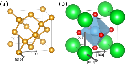
Figure 1: Unit cell of (a) the diamond-structure and (b) the c-SrTiO₃ perovskite simulated materials. Grey arrows illustrate the crystallographic directions that form the Cartesian axes.

The above derivation, in addition to settling the existing formal issues regarding HWRV’s method, also allows for a more compact expression of our second sum rule. To that end, note that the strain derivative of the stress is related to Oganov’s definition via Oganov (accessed December 13, 2021); Hamann et al. (2005)

$$\frac{\partial\sigma_{\alpha\gamma}}{\partial u_{\beta\delta}}=\bar{C}_{\alpha\gamma,\beta\delta}^{\rm Og}-\delta_{\beta\delta}S_{\alpha\gamma}.$$ (62)

By combining this result with Eq. (60), we obtain an equivalent formulation of Eq. (58) as

$$\frac{1}{\Omega}\sum_{\kappa}\bar{C}^{\kappa}_{\alpha\gamma,\beta\delta}=\bar{\cal{C}}_{\alpha\gamma,\beta\delta}=\frac{\partial\sigma_{\beta\delta}}{\partial u_{\alpha\gamma}}.$$ (63)

The strain derivative of the stress tensor is indicated by HWRV as “improper” elastic tensor. Here we have seen that there are many flavors of the elastic tensor so the distinction between what should be regarded as a “proper” and “improper” definition needs to be revised in light of the above results. We shall call “proper” any definition that respects the full symmetries of the elastic tensor under the most general (anisotropic stress) conditions. Only ${\bf C^{\rm La}}$ and ${\bf C^{\rm HWRV}}$ fulfill this requirement, although we regard ${\bf C^{\rm La}}$ as a physically more useful choice. [It lends itself more easily to higher-order generalizations of the elastic energy, see e.g. Ref. Cao et al., 2018.] The other definitions, ${\bf C^{\rm un}}$, ${\bf C^{\rm Og}}$ and $\bm{\mathcal{C}}$, are all “improper” in the above sense.

Table 1: Breakdown of the linearly independent bulk flexoelectric coefficients (in nC/m) of Si, diamond (C) and c-SrTiO₃. The first four columns show the contributions arising from the different terms in Eqs. (2). The total flexoelectric tensor is shown in the fifth column. The rightmost column shows the open-circuit flexovoltages (in V). Highlighted quantities have been directly obtained with the formalism and implementation presented in this work.

		$\bm{\bar{\mu}}$	$\bm{P}^{(1)}\bm{\Gamma}$	$\bm{\bar{C}}$	$\bm{\Phi}^{(1)}\bm{\Gamma}$	$\bm{\mu}$	$\bm{\varphi}$
	$xx,xx$	$-$1.399				$-$1.399	$-$12.002
Si	$xx,yy$	$-$1.036				$-$1.036	$-$8.894
	$xy,xy$	$-$0.188	$-$0.107			$-$0.296	$-$2.538
	$xx,xx$	$-$0.995				$-$0.995	$-$19.683
C	$xx,yy$	$-$0.787				$-$0.787	$-$15.567
	$xy,xy$	$-$0.131	$-$0.009			$-$0.141	$-$2.783
	$xx,xx$	$-$0.891		$-$181.950		$-$182.841	$-$18.583
SrTiO3	$xx,yy$	$-$0.832		$-$157.953		$-$158.785	$-$16.138
	$xy,xy$	$-$0.083		$-$19.310		$-$19.392	$-$1.971

VI Implementation and results

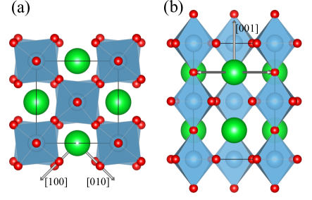
Figure 2: (a) Top and (b) side view of the unit cell employed in the simulation of t-SrTiO₃. Grey arrows illustrate the crystallographic directions that form the Cartesian axes.

VI.1 Implementation details

The calculation of the tensors $\Phi^{(1,\gamma)}_{\kappa\alpha,\kappa^{\prime}\beta}$ and $\bar{C}^{\kappa}_{\alpha\gamma,\beta\delta}$ by means of Eqs. (29) and (75), respectively, has been implemented in the abinit open-source software. Gonze et al. (2009, 2016); Romero et al. (2020) In addition, the post-processing computations in order to obtain the indirect contributions to the flexoelectric tensor (i.e., the rhs terms of Eqs. (2)) have been implemented in the anaddb tool. These developments, together with the ones associated with our preceding work, Royo and Stengel (2019) provide a new functionality, recently released for its public usage in the v9 version of abinit, Romero et al. (2020) that allows a non-specialized user to readily obtain the complete bulk flexoelectric tensor for any time-reversal symmetric crystalline insulator.

The internal strain $\Gamma^{\kappa}_{\rho\beta\delta}$ is necessary to build the indirect terms of Eqs. (2). As we have seen in Sec. II, its calculation first requires to compute the piezoelectric force-response tensor, $\Lambda_{\alpha,\beta\delta}^{\kappa}$. The latter, in turn, can be directly obtained from a uniform strain linear-response calculation Hamann et al. (2005), as implemented in the abinit package, or from the sublattice summation of the first moment of the FC matrix via Eq. (56). In our implementation we have adopted the second option for consistency with the other quantities entering the flexoelectric tensor. In any case, we test numerically their mutual relationship, Eq. (56), to validate our implementation of $\Phi^{(1,\gamma)}_{\kappa\alpha,\kappa^{\prime}\beta}$. To calculate the improper contributions of Eqs. (56) and (57) we use the standard Nielsen and Martin (1985) formulation of forces and stress as implemented in abinit. The pseudoinverse of the FC matrix $\widetilde{\Phi}^{(0)}_{\kappa\rho,\kappa^{\prime}\sigma}$ is constructed following the prescriptions of Ref. Wu et al., 2005.

VI.2 Computational parameters

Our numerical results are obtained using the DFT and DFPT implementations of abinit v9.0.4 with the Perdew-Wang Perdew and Wang (1992) parametrization of the LDA. We use norm-conserving pseudopotentials from the Pseudo Dojo, van Setten et al. (2018) after regenerating them without exchange-correlation nonlinear core corrections using the ONCVPSP software. Hamann et al. (1979); Hamann (1989) The unit cells employed for our simulations on cubic- and tetragonal-structure materials are illustrated in Figs. 1 and 2, respectively.

For our calculations on Si and diamond, we use the primitive 2-atom cells with a cell parameter of 10.182 bohr (Si) and 6.673 bohr (diamond), a plane-wave cutoff of 20 Ha (Si) and 40 Ha (diamond) and a BZ sampled with a Monkhorst-Pack (MP) mesh of $12\times 12\times 12$ k points. For our calculations of cubic SrTiO₃ we use a 5-atom primitive cell, with a lattice constant of $a=7.288$ bohr, a plane-wave cutoff of 80 Ha and a BZ sampling of $10\times 10\times 10$ k points. We represent the tetragonal structure with a 20-atom cell (cell parameters: $a=10.271$, $c=14.639$ bohr). To facilitate the comparison to the cubic structure we align the pseudocubic [100], [010] and [001] directions (the latter corresponding to the tilt axis) with the Cartesian $x$, $y$ and $z$ axes, respectively. We use a BZ sampling of ($6\times 6\times 4$) k points in this case.

Table 2: List of parameters driving the indirect contribution to flexoelectricity in the diamond structure: first moment of the FC ($\phi$, units are $10^{-3}$ Ha/bohr), piezoelectric force-response from a HWRV calculation Hamann et al. (2005) ($\lambda$, $10^{-3}$ Ha/bohr), frequency of the Raman-active mode ($\omega_{T_{1g}}$, cm^-1), internal strain ($\gamma$, $10^{-3}$ bohr) and the electronic polarization induced by an atomic-displacement gradient ($p$, $10^{-3}$ e/bohr²).

	$\phi$	$\lambda$	$\omega_{T_{1g}}$	$\gamma$	$p$
Si	190.272	190.273	512.555	681.428	25.961
C	79.060	79.071	1323.381	99.315	15.355

VI.3 Cubic crystals

We start by testing the performance of our implementation on three representative insulators with cubic crystal structure: Si, diamond and SrTiO₃. The main motivation originates from the availability of first-principles results in the literature on both the first moment of the FC matrix and the CI flexoelectric force-response tensor. [For details on the purely electronic response functions contributing to the flexoelectric tensor, i.e., $\bar{\mu}_{\alpha\gamma,\beta\delta}$ and $P_{\alpha,\kappa^{\prime}\rho}^{(1,\gamma)}$ in Eq. (2a), see Ref. Royo and Stengel, 2019.] Note that, due to cubic symmetry, the flexoelectric tensor in this materials set has only three independent components; following earlier works, we shall refer to them as longitudinal ($\mu_{xx,xx}$), transverse ($\mu_{xx,yy}$) and shear ($\mu_{xy,xy}$). In Table LABEL:Tab_cubic_flexo we present a summary of the results for the three materials; we provide their detailed analysis hereafter.

VI.3.1 Diamond-structure semiconductors

Table 3: Linearly-independent components of the silicon and diamond CI flexoelectric force-response tensors (in eV) and of the CI elastic tensors (in GPa). The latter are calculated with the sublattice summation of the flexoelectric force-response tensor (Eq. (11)) and with the HWRV approach. Hamann et al. (2005)

		$xx,xx$	$xx,yy$	$xy,xy$
	$\bar{C}^{\kappa}_{\alpha\gamma,\beta\delta}$	19.670	7.678	12.880
Si	$\mathcal{\bar{C}}_{\alpha\gamma,\beta\delta}$	161.163	62.903	105.532
	$\mathcal{\bar{C}}^{\rm HWRV}_{\alpha\gamma,\beta\delta}$	161.169	62.907	105.533
	$\bar{C}^{\kappa}_{\alpha\gamma,\beta\delta}$	38.148	4.999	20.712
C	$\mathcal{\bar{C}}_{\alpha\gamma,\beta\delta}$	1110.651	145.560	603.005
	$\mathcal{\bar{C}}^{\rm HWRV}_{\alpha\gamma,\beta\delta}$	1110.899	145.903	602.955

Due to their purely covalent nature, the Born effective charge tensor identically vanishes in both diamond and Si, which implies that the lattice-mediated contribution to the flexoelectric tensor vanishes as well. The purely electronic part, Eq. (2a), consists of a clamped-ion contribution Royo and Stengel (2019) and an additional term originated from the strain coupling of the Raman-active optical mode; we shall focus on the latter in the following. Via a symmetry analysis, we find that the relevant tensors are governed by one parameter each,

$$P_{\alpha,\kappa\rho}^{(1,\gamma)} = (-1)^{\kappa+1}\,p\,|\varepsilon_{\alpha\rho\gamma}|,$$ (64a)

$$\Phi^{(1,\delta)}_{\kappa\rho,\kappa^{\prime}\beta} = (-1)^{\kappa+1}\,(1-\delta_{\kappa\kappa^{\prime}})\,\phi\,|\varepsilon_{\rho\beta\delta}|,$$ (64b)

$$\Lambda^{\kappa}_{\rho\beta\delta} = (-1)^{\kappa+1}\,\lambda\,|\varepsilon_{\rho\beta\delta}|,$$ (64c)

$$\Gamma^{\kappa}_{\rho\beta\delta} = (-1)^{\kappa+1}\,\gamma\,|\varepsilon_{\rho\beta\delta}|,$$ (64d)

where $\varepsilon_{\alpha\beta\gamma}$ is the Levi-Civita tensor. The calculated values reported in Table 2 show that the piezoelectric force-response tensor sum rule at mechanical equilibrium, Eq. (7), is fulfilled to a very high degree of accuracy in both materials. [Due to Eqs. (64b) and (64c), this sum rule trivially reduces to an equality: $\phi=\lambda$.] Our results for $\gamma$ are in fair agreement with the value of $\gamma=0.72,0.14$ bohr, respectively for Si and C, quoted by Hong and Vanderbilt Hong and Vanderbilt (2013). Our values of $p$, however, markedly differ with those of Ref. Hong and Vanderbilt, 2013; this is likely due to a technical issue with the calculations reported therein Vanderbilt . Note that the $p$ coefficients in both Si and C are related to the dynamical quadrupoles $Q$ of Ref. Royo and Stengel, 2019 via $p=Q/(2\Omega)$.

Based on Eq. (2a), the indirect (“mixed”) contribution to the flexoelectric tensor in Si and C can be written as

$$\mu^{\rm ind}_{\alpha\gamma,\beta\delta}=-2p\gamma|\delta_{\alpha\beta}\delta_{\gamma\delta}-\delta_{\alpha\delta}\delta_{\gamma\beta}|,$$ (65)

yielding a value of $\mu^{\rm ind}_{\alpha\beta,\alpha\beta}=\mu^{\rm ind}_{\alpha\beta,\beta\alpha}=-2p\gamma$ for the shear components and zero otherwise.

In Table LABEL:Tab_cubic_flexo we summarize the results for the bulk flexoelectric tensor in Si and C. The values shown indicate that $\mu^{\rm ind}$ is significantly smaller than the purely electronic contribution $\bar{\mu}$, especially in C. [$\mu^{\rm ind}$ accounts for $\sim 37\%$ and $\sim 6\%$ of the total shear coefficient in Si and C, respectively.] We ascribe the smallness of the response in diamond to the stiffness of the Raman mode (see Table 2), which leads to a strongly suppressed internal-strain parameter $\Gamma$ compared to Si. The electronic polarization parameter $P$, on the other hand, appears comparable in both materials.

Even if the force-response tensor does not result in a contribution to the flexoelectric polarization, it is still interesting to analyze it in light of the sum rules discussed in Sec. II.2. We find that, at the CI level, $\bar{C}^{\kappa}_{\alpha\gamma,\beta\delta}$ is symmetric with respect to the atomic index $\kappa$; thus, Eq. (11) reduces again (within the zero-stress regime that we test here) to an equality, $\bar{\mathcal{C}}=2\bar{C}^{\kappa=1}/\Omega$. The values reported in Table LABEL:Tab_diam_forces show that this sum rule holds to an excellent degree of accuracy, confirming the correctness and numerical quality of our implementation.

Table 4: Five top rows: Linearly-independent CI flexoelectric force-response tensor coefficients, $\bar{C}^{\kappa}_{\alpha\gamma,\beta\delta}$, of c-SrTiO₃ (in eV). Data between brackets is from Ref. Stengel and Vanderbilt, 2016. Two bottom rows: CI elastic coefficients (in GPa) calculated with the sublattice summation of the flexoelectric force-response tensor (Eq. (11)) and with the HWRV approach Hamann et al. (2005).

Atom	$xx,xx$	$xx,yy$	$xy,xy$
Sr	$-$25.0 ($-$24.9)	$-$28.5 ($-$28.7)	7.7 (7.9)
Ti	$-$66.9 ($-$67.9)	$-$102.2 ($-$102.3)	3.5 (3.8)
O1	34.9 (35.2)	30.7 (30.9)	17.2 (17.3)
O2	34.9 (35.2)	42.3 (42.3)	15.3 (15.3)
O3	159.9 (159.3)	97.4 (97.4)	$-$1.0 ($-$0.9)
$\mathcal{\bar{C}}_{\alpha\gamma,\beta\delta}$	384.842	110.680	119.041
$\mathcal{\bar{C}}^{\rm HWRV}_{\alpha\gamma,\beta\delta}$	384.848	110.671	119.039

VI.3.2 Cubic SrTiO₃

In cubic SrTiO₃ (c-SrTiO₃), the absence of free Wyckoff parameters results in vanishing ${\bm{P}^{(1)}}$ and ${\bm{\Phi}^{(1)}}$ tensors; this implies that the indirect contributions to the flexoelectric polarization vanish as well. The most striking feature emerging from our results (Table LABEL:Tab_cubic_flexo) is that the lattice-mediated contribution largely dominates the overall response in this material, accounting for more than $99\%$ of the total in all three tensorial components. This is consistent with our expectations and the results of earlier works Stengel (2014, 2016): cubic SrTiO₃, being an incipient ferroelectric, has a polar mode (of $T_{1u}$ symmetry) with low frequency (45.738 cm^-1) and strong dipolar character. This mode mediates a huge electrical response to any symmetry-allowed perturbation (for example, the static dielectric constant nearly diverges in SrTiO₃ at low temperature), dominating over other degrees of freedom. In the experimental context, in ferroelectrics and incipient ferroelectrics it has become common practice to divide the measured flexoelectric coefficients by the static dielectric constant, and thus obtain a temperature-independent physical quantity known as flexovoltage. For this reason, we also report these coefficients ($\varphi$) in Table LABEL:Tab_cubic_flexo, in units of voltage.

Consistent with earlier works, the longitudinal and transverse components of the flexoelectric tensor (Table LABEL:Tab_cubic_flexo) are similar in magnitude, and both much larger than the shear component. This is largely a consequence of using the macroscopic electrostatic potential as the (arbitrary) energy reference when imposing short-circuit EBC (see e.g. Sec. II.3), and should not be interpreted as a real physical effect. Indeed, for the case of c-SrTiO₃, it was shown Stengel (2013b) that all three types of strain-gradient deformations yield a quantitatively similar flexoelectric response when other energy references, such as the valence- and conduction-band edges, are adopted. Discussing the details on how the choice of the energy reference affects each individual contribution appearing in Eqs. (2) goes beyond the scopes of this work, and will be covered in a future publication.

Table 5: Selected piezoelectric force-response coefficients (in $10^{-3}$ Ha/bohr) of the distorted SrTiO₃ system. The first column shows results from a HWRV Hamann et al. (2005) metric-tensor calculation, while the second and third columns show the sublattice summation of the first moment of the FC matrix neglecting (Eq. (7)) and including (Eq. (56)) the improper contribution mentioned in the text.

	HWRV	Eq. (7)	Eq. (56)
$\Lambda^{\rm{Sr}}_{xxx}$	97.616	111.596	97.616
$\Lambda^{\rm{Sr}}_{xyy}$	86.323	86.3228	86.323
$\Lambda^{\rm{Sr}}_{xxz}$	$-$14.060	$-$14.060	$-$14.060
$\Lambda^{\rm{Sr}}_{xzx}$	$-$14.060	$-$7.421	$-$14.060
$\Lambda^{\rm{Ti}}_{yyy}$	29.021	16.800	29.021
$\Lambda^{\rm{Ti}}_{yzz}$	$-$360.977	$-$360.977	$-$360.977
$\Lambda^{\rm{Ti}}_{yyx}$	$-$18.556	$-$18.556	$-$18.556
$\Lambda^{\rm{Ti}}_{yxy}$	$-$18.556	$-$56.446	$-$18.556
$\Lambda^{\rm{O}}_{zzz}$	1887.068	2110.762	1887.065
$\Lambda^{\rm{O}}_{zxx}$	168.414	168.414	168.414
$\Lambda^{\rm{O}}_{zzy}$	262.311	262.309	262.309
$\Lambda^{\rm{O}}_{zyz}$	262.311	276.029	262.309

In Table 4 we show our calculated CI flexoelectric force-response coefficients, and compare them with the ones reported in Ref. Stengel and Vanderbilt, 2016, where they are directly obtained from the second moments of the FC (as e.g in Eq. (5b)). As evident from the data presented in the table, our results compare quite well with the published ones despite the fact that a different set of pseudopotentials and cell parameters are employed in the two calculations. In the two bottom rows of Table 4 we also show the CI elastic coefficients of c-SrTiO₃ calculated via the elastic sum rule Eq. (11) together with the corresponding values obtained with the HWRV calculation. The comparison between the two sets of data evidences, one more time, an excellent agreement.

Table 6: Selected CI elastic tensor coefficients (in GPa) of a distorted SrTiO₃ system. Different columns show the elastic tensor as obtained from different approaches (from left to right): sublattice summation of flexoelectric force-response tensor (Eq. (11)), right-hand side of Eq. (58), HWRV, Hamann et al. (2005) and Lagrange as calculated from HWRV (Eq. (61)).

	$\cal{\bar{C}_{\alpha\gamma,\beta\delta}}$	Eq. (58)	$\mathcal{\bar{C}}^{\rm HWRV}_{\alpha\gamma,\beta\delta}$	$\bar{C}^{\rm La}_{\alpha\gamma,\beta\delta}$
$xx,xx$	219.440	219.432	227.631	211.242
$yy,zz$	164.706	164.696	113.210	113.200
$zz,yy$	103.990	103.981	113.209	113.200
$xy,xy$	120.673	120.674	120.159	111.455
$yx,xy$	119.645	119.645	120.159	111.455
$yz,yz$	45.559	45.560	75.917	97.056
$yz,zy$	45.559	45.560	75.917	45.560

VI.4 Distorted SrTiO₃

In this section, we numerically test the forces- and stress-mediated improper contributions to the sum rules derived in Sec. V. To this end, we study a fictitious SrTiO₃ lattice where we artificially create finite stresses and forces. In particular, we randomly distort in the range of $\pm 5\%$ the primitive vectors and the relative atomic coordinates from their equilibrium values in the 5-atom primitive cubic cell.

First, we focus on the piezoelectric force-response tensor by comparing the outcomes of three different calculations: i) the HWRV Hamann et al. (2005) one, which we regard as our reference, ii) the sublattice summation of the $\Phi^{(1,\gamma)}_{\kappa\alpha,\kappa^{\prime}\beta}$ tensor [Eq. (7)], and iii) the same sublattice summation of $\Phi^{(1,\gamma)}_{\kappa\alpha,\kappa^{\prime}\beta}$, but including the improper contribution from the residual forces [Eq. (56)]. The results shown in Table 5 nicely confirm our formal prediction: the sublattice sum of $\Phi^{(1,\gamma)}_{\kappa\alpha,\kappa^{\prime}\beta}$ coincides with $\Lambda_{\alpha,\beta\delta}^{\kappa}$ only if the improper contribution is taken into account, otherwise the error can be large, and the expected symmetry in the strain indices ($\beta\delta$) is clearly violated.

Table 7: Breakdown of the linearly-independent flexoelectric coefficients (in nC/m) of t-SrTiO₃. The rightmost column shows the open-circuit flexovoltages (in V). Data are presented following the same scheme as in Table LABEL:Tab_cubic_flexo

	$\bm{\bar{\mu}}$	$\bm{P}^{(1)}\bm{\Gamma}$	$\bm{\bar{C}}$	$\bm{\Phi}^{(1)}\bm{\Gamma}$	$\bm{\mu}$	$\bm{\varphi}$
$xx,xx$	$-$0.946	0.056	$-$68.865	3.516	$-$66.239	$-$18.086
$zz,zz$	$-$0.898	$-$0.013	$-$55.841	$-$2.507	$-$59.259	$-$18.765
$xx,yy$	$-$0.786	0.052	$-$55.977	3.416	$-$53.294	$-$14.551
$xx,zz$	$-$0.830	$-$0.041	$-$58.133	$-$2.626	$-$61.631	$-$16.828
$zz,xx$	$-$0.841	0.017	$-$49.897	3.308	$-$47.413	$-$15.014
$xy,xy$	$-$0.028	0.002	$-$4.091	0.313	$-$3.805	$-$1.039
$xz,xz$	$-$0.079	0.023	$-$6.796	$-$1.292	$-$8.144	$-$2.224
$zx,xz$	$-$0.081	0.013	$-$5.468	$-$1.706	$-$7.242	$-$2.293

Next, we study (at the CI level) the second-order elastic coefficients of the distorted SrTiO₃ crystal as obtained from the different strain tensor definitions of Sec. V, and compare them to the sublattice summation of the CI flexeoelectric force-response tensor [Eq. (11)]. In particular, we consider: (i) HWRV Hamann et al. (2005) ($\mathcal{\bar{C}}^{\rm HWRV}_{\alpha\gamma,\beta\delta}$) (ii) Lagrange ($\bar{C}^{\rm La}_{\alpha\gamma,\beta\delta}$), which we obtain from $\mathcal{\bar{C}}^{\rm HWRV}_{\alpha\gamma,\beta\delta}$ via Eq. (61) (iii) $\cal{\bar{C}_{\alpha\gamma,\beta\delta}}$, given by the sum of $C^{\kappa}_{\alpha\gamma,\beta\delta}$ [Eq. (11)] (iv) the same sublattice sum of $C^{\kappa}_{\alpha\gamma,\beta\delta}$, but including the improper contribution [Eq. (58)] from the residual stress. The results are summarized in Table 6. As a general observation, it is clear that the presence of residual stresses breaks the equivalence between the different versions of the elastic tensor discussed in Sec. V. The data shown in the first column confirm that $\cal{\bar{C}_{\alpha\gamma,\beta\delta}}$ is only symmetric with respect to the permutation of the second pair of indices ($\beta,\delta$); on the other hand, the symmetries with respect to ($\alpha,\gamma$) and with respect to an exchange of the last two with the first two pair of indices are both broken. In contrast, the HWRV and Lagrange elastic coefficients, respectively shown in the third and fourth columns, manifestly enjoy the whole set of symmetries of a proper elastic tensor. Finally, the excellent match between the data of the first two columns numerically demonstrates the generalized elastic sum rule expressed in Eq. (58).

VI.5 Tetragonal SrTiO₃

SrTiO₃ undergoes, at $T_{\rm{}_{c}}\approx 105$ K, a cubic-to-tetragonal phase transition driven by the antiferrodistortive tilts of the oxygen octahedra, leading to a $I4/mcm$ ground state ($a^{0}a^{0}c^{-}$ in Glazer notation). After the transition, the tilt modes become Raman active, and therefore mediate, in principle, an indirect contribution to the flexoelectric tensor as discussed in Sec. II.1. Interestingly, a marked change in the flexoelectric response of SrTiO₃ was reported experimentally Zubko et al. (2007) upon cooling the sample below $T_{\rm{}_{c}}$, which suggests an important contribution of the tilt modes. From this perspective, tetragonal SrTiO₃ (t-SrTiO₃) appears as an excellent physical example to showcase our methods.

Our calculated values for the flexoelectric coefficients, together with their decompositions into the contributions described in Sec. II.1, are shown in Table 7. (As above, we also verified that the sum rules described in the previous paragraphs are accurately fulfilled; results are not shown.) The larger number of independent components (8, compared to only 3 in the $Pm\bar{3}m$ phase) is due to the lower symmetry of the tetragonal cell. The CI coefficients $\bar{\mu}$ show little variation compared to their cubic counterparts, shown in Table LABEL:Tab_cubic_flexo. On the other hand, the direct LM contributions are systematically suppressed by about a factor of three. This is simply explained by the stiffening of the lowest-lying transverse polar modes, whose calculated frequencies are $\omega_{E_{u}}=78.034$ cm^-1 and $\omega_{A_{2u}}=87.073$ cm^-1 for polarization perpendicular ($E_{u}$) or parallel ($A_{2u}$) to the tilt axis. (As we stated earlier, these modes are primarily responsible for the large LM response in SrTiO₃, and their contribution to the flexoelectric polarization scales like the inverse square of their frequency Stengel (2016).) Such an interpretation is supported by our analysis of the bulk open-circuit voltage: all type of deformations result in a similar value (cf. rightmost columns of Tables LABEL:Tab_cubic_flexo and 7) in both the cubic and the tetragonal phase, confirming that the suppression is almost entirely due to the smaller dielectric susceptibility of the latter.

As anticipated, we obtain finite indirect contributions to both the electronic and lattice-mediated parts (see data in second and fourth columns of Table 7). Although these are comparatively smaller in magnitude than the CI contributions, they account for a nonnegligible fraction of the total coefficients. (Note, e.g., the $\mu_{xz,xz}$ case wherein the indirect contributions amount to $\sim 41$% and $\sim 16$% of the total electronic and lattice-mediated parts, respectively.) To understand the origin of such contributions, it is useful to identify the lattice modes whose coupling to strain is strongest. A mode decomposition of the internal-strain response tensor $\Gamma$ shows that the lattice response to a uniform strain is dominated by tilts, via a nonlinear coupling term known as rotostriction. A gradient of the tilts, in turn, produces a polarization via the “rotopolar” coupling, Schiaffino and Stengel (2017) which is activated in presence of a uniform tilt. While promising in light of the observations of Ref. Zubko et al., 2007, a quantitative analysis of our results in terms of these mechanisms goes, however, beyond the scopes of the present work, and will be the topic of a forthcoming publication.

VII Conclusions and outlook

We have derived the long-wave DFPT Royo and Stengel (2019) formulas to calculate the two spatial-dispersion quantities necessary to build the lattice-mediated contributions to the bulk flexoelectric tensor. These are, the first real-space moment of the interatomic FC matrix and the CI flexoelectric force-response tensor. We have also generalized to crystals out of mechanical equilibrium the sum rules that relate the latter quantities to the established theory of linear elasticity. We have implemented our formalism in the ABINIT package, thus completing our earlier developments in the context of the electronic flexoelectric tensor. Royo and Stengel (2019) We carried out extensive numerical tests to benchmark our results against the literature, and demonstrated the performance of our method by calculating the bulk flexoelectric tensor of the low-temperature tetragonal structure of SrTiO₃.

This work culminates a series of theoretical advances carried out during the last decade on the first-principles theory of flexoelectricity and opens the way to the systematic calculation of the bulk flexoelectric tensor for any insulating crystal or nanostructure. We expect this work to greatly facilitate the construction of higher-level theories involving gradient-mediated effects. Indeed, both the first moment of the FC and the flexoelectric force-response tensor (via its reformulation as a flexocoupling Stengel (2016)) are the necessary parameters in order to describe, respectively, rotopolar and flexolectric couplings within a continuum thermodynamic functional Schiaffino and Stengel (2017) or an effective Hamiltonian. Ponomareva et al. (2012) Surface contributions, albeit not considered here, can be readily incorporated by using our formalism in a supercell calculation of a material slab; this has been shown in Ref. Springolo et al., 2021 for a set of two-dimensional materials under a flexural deformation.

On the methodological front, work is currently under way to extend our formalism, both in regards to technical details of the implementation (e.g., for the usability of the generalized-gradient approximation or nonlinear core corrections in the calculation of the flexoelectric coefficients), and in the description of related spatial dispersion properties (e.g. natural optical activity or acoustical activity) based on similar methodologies. Reports on progress along these lines will be presented in a forthcoming publication.

Appendix A q derivatives of Ewald energy

The ion-ion Ewald contribution to the FC matrix can be found in Ref. Gonze and Lee, 1997b. Here, we use a slightly different formulation since we assume the same sublattice-dependent phase factor for the perturbation that was conveniently taken in our previous works (see, e.g., Refs. Stengel, 2013a; Royo and Stengel, 2019). The conversion from Ref. Gonze and Lee, 1997b formula simply consists in multiplying it by $e^{i\mathbf{q}(\bm{\tau}_{\kappa}^{\prime}-\bm{\tau}_{\kappa})}$, which yields

$$\begin{split}&E_{{\rm Ew},\mathbf{q}}^{\tau^{*}_{\kappa\alpha}\tau_{\kappa^{\prime}\beta}}=Z_{\kappa}Z_{\kappa^{\prime}}\Big{[}\frac{4\pi}{\Omega}\sum_{\mathbf{G}}\frac{(G+q)_{\alpha}(G+q)_{\beta}}{(G+q)^{2}}\,e^{i\mathbf{G}(\bm{\tau}_{\kappa}-\bm{\tau}_{\kappa^{\prime}})}\,\\ &\quad e^{-\frac{(G+q)^{2}}{4\Lambda^{2}}}-\sum_{a}\Lambda^{3}\,e^{i\mathbf{q}{\bf d}_{a,\kappa\kappa^{\prime}}}\,H^{iso}_{\alpha\beta}(\Lambda{\bf d}_{a,\kappa\kappa^{\prime}})\\ &\quad-\frac{4}{3\sqrt{\pi}}\Lambda^{3}\delta_{\kappa\kappa^{\prime}}e^{i\mathbf{q}(\bm{\tau}_{\kappa^{\prime}}-\bm{\tau}_{\kappa})}\Big{]}.\end{split}$$ (66)

Here $Z_{\kappa}$ is the nuclear charge, ${\bf d}_{a,\kappa\kappa^{\prime}}={\bf R}_{a}+\bm{\tau}_{\kappa^{\prime}}-\bm{\tau}_{\kappa}$, $\Lambda$ is a range-separation parameter (setting the Gaussian width) with momentum units that can adopt any value to accelerate the sums convergence, and the specific formula for $H^{iso}_{\alpha\beta}$ is shown in Eq. (25) of Ref. Gonze and Lee, 1997b. By differentiating the above formula, we arrive at the following q gradients of the Ewald contribution (at q=0).

The first q gradient is given by,

$$\begin{split}&E_{{\rm Ew},\gamma}^{\tau^{*}_{\kappa\alpha}\tau_{\kappa^{\prime}\beta}}=Z_{\kappa}Z_{\kappa^{\prime}}\Bigg{\{}\frac{4\pi}{\Omega}\sum_{{\bf G}}e^{i{\bf G}(\bm{\tau}_{\kappa}-\bm{\tau}_{\kappa^{\prime}})}\,e^{-\frac{G^{2}}{4\Lambda^{2}}}\times\\ &\quad\Bigg{[}\frac{\Big{(}\delta_{\alpha\gamma}G_{\beta}+\delta_{\beta\gamma}G_{\alpha}\Big{)}}{G^{2}}-\frac{2G_{\alpha}G_{\beta}G_{\gamma}}{G^{4}}-\frac{1}{2\Lambda^{2}}\frac{G_{\alpha}G_{\beta}G_{\gamma}}{G^{2}}\Bigg{]}\\ &\quad-\sum_{a}\Lambda^{3}i\,d_{a,\kappa\kappa^{\prime},\gamma}\,H^{iso}_{\alpha\beta}(\Lambda{\bf d}_{a,\kappa\kappa^{\prime}})\Bigg{\}}.\end{split}$$ (67)

The second q gradient is given by,

$$\begin{split}&E_{{\rm Ew},\gamma\delta}^{\tau^{*}_{\kappa\alpha}\tau_{\kappa^{\prime}\beta},{\rm I}}=Z_{\kappa}Z_{\kappa^{\prime}}\Bigg{\{}\frac{4\pi}{\Omega}\sum_{{\bf G}}e^{i{\bf G}(\bm{\tau}_{\kappa}-\bm{\tau}_{\kappa^{\prime}})}\,\frac{e^{-\frac{G^{2}}{4\Lambda^{2}}}}{G^{2}}\times\\ &\quad\Bigg{[}\delta_{\alpha\gamma}\delta_{\beta\delta}+\delta_{\beta\gamma}\delta_{\alpha\delta}-\Big{(}\frac{1}{2\Lambda^{2}}+\frac{2}{G^{2}}\Big{)}\Big{(}G_{\alpha}G_{\beta}\delta_{\gamma\delta}\\ &\quad+G_{\delta}(\delta_{\alpha\gamma}G_{\beta}+\delta_{\beta\gamma}G_{\alpha})+G_{\gamma}(\delta_{\alpha\delta}G_{\beta}+\delta_{\beta\delta}G_{\alpha})\Big{)}\\ &\quad+\Big{(}\frac{1}{4\Lambda^{4}}+\frac{2}{\Lambda^{2}G^{2}}+\frac{8}{G^{4}}\Big{)}G_{\alpha}G_{\beta}G_{\gamma}G_{\delta}\Bigg{]}\\ &\quad+\sum_{a}\Lambda^{3}\,(d_{a,\kappa\kappa^{\prime}})_{\gamma}(d_{a,\kappa\kappa^{\prime}})_{\delta}\,H^{iso}_{\alpha\beta}(\Lambda{\bf d}_{a,\kappa\kappa^{\prime}})\Bigg{\}}.\end{split}$$ (68)

Appendix B Second q derivative of atomic displacement Hamiltonian

The first-order atomic-displacement Hamiltonian consists in a local and a non-local pseudopotential term. The explicit formulas of both contributions, as well as their first q derivative (at q=0) were reported in our preceeding paper. Royo and Stengel (2019) By further differentiation, we arrive at the second q gradients of the perturbation, which are necessary to compute the geometric contribution entering the CI flexoelectric force-response tensor (see Eqs. (39) and (40)).

The local part of the pseudopotential is

$$\begin{split}&V_{\gamma\delta}^{{\rm loc},\,\tau_{\kappa\alpha}}({\bf G})=-\frac{i}{\Omega}e^{-i{\bf G}\tau_{\kappa}}\times\\ &\quad\Bigg{(}\frac{v_{\kappa}^{\rm loc}(G)^{\prime}}{G}\Big{(}\delta_{\alpha\delta}G_{\gamma}+\delta_{\alpha\gamma}G_{\delta}+\delta_{\gamma\delta}G_{\alpha}-\frac{G_{\alpha}G_{\delta}G_{\gamma}}{G^{2}}\Big{)}\\ &\quad+\frac{v_{\kappa}^{\rm loc}(G)^{\prime\prime}}{G^{2}}G_{\alpha}G_{\delta}G_{\gamma}\Bigg{)},\end{split}$$ (69)

where $G=|{\bf G}|$, $v_{\kappa}^{\rm loc}(G)^{\prime}$ and $v_{\kappa}^{\rm loc}(G)^{\prime\prime}$ are the first and second derivatives of the spherical atomic pseudopotential. The separable part of the pseudopotential is

$$\begin{split}&V^{sep,\tau_{\kappa\alpha}}_{{\bf k},\gamma\delta}({\bf G},{\bf G}^{\prime})=-\frac{i}{\Omega}\sum_{\mu}e_{\mu\kappa}\,e^{-i({\bf G}-{\bf G}^{\prime})\bm{\tau}_{\kappa}}\times\\ &\qquad\Bigg{[}\delta_{\alpha\gamma}\zeta_{\mu\kappa,\delta}({\bf k}+{\bf G})\zeta^{*}_{\mu\kappa}({\bf k}+{\bf G}^{\prime})\\ &\qquad+\delta_{\alpha\delta}\zeta_{\mu\kappa,\gamma}({\bf k}+{\bf G})\zeta^{*}_{\mu\kappa}({\bf k}+{\bf G}^{\prime})\\ &\qquad+(k_{\alpha}+G_{\alpha})\zeta_{\mu\kappa,\gamma\delta}({\bf k}+{\bf G})\zeta^{*}_{\mu\kappa}({\bf k}+{\bf G}^{\prime})\\ &\qquad-\zeta_{\mu\kappa,\gamma\delta}({\bf k}+{\bf G})(k_{\alpha}+G_{\alpha}^{\prime})\zeta^{*}_{\mu\kappa}({\bf k}+{\bf G}^{\prime})\Bigg{]}.\end{split}$$ (70)

with $\zeta_{\mu\kappa,\gamma}({\bf k}+{\bf G})$ and $\zeta_{\mu\kappa,\gamma\delta}({\bf k}+{\bf G})$ being the first and second ${\bf q}$ derivatives along the $\gamma$ and $\delta$ Cartesian directions of the separable nonlocal projector.

Appendix C Phonon–metric stationary functional

At the end of Sec. IV.2, we have shown that the square-bracket tensor can be obtained from the sum of a stationary and a nonvariational second-order functionals,

$$[\alpha\beta,\gamma\delta]^{\kappa}=\frac{1}{2}\left(E^{\tau^{*}_{\kappa\alpha}(\beta)}_{{\rm st},\gamma\delta}+E^{\tau^{*}_{\kappa\alpha}(\beta)}_{{\rm nv},\gamma\delta}\right).$$ (71)

Following the arguments of Ref. Royo and Stengel, 2019, the stationary part needs to be symmetrized with respect to $\gamma$ and $\delta$ as

$$E^{\tau^{*}_{\kappa\alpha}(\beta)}_{{\rm st},\gamma\delta}=\widetilde{E}^{\tau^{*}_{\kappa\alpha}(\beta)}_{{\rm st},\gamma\delta}+\widetilde{E}^{\tau^{*}_{\kappa\alpha}(\beta)}_{{\rm st},\delta\gamma},$$ (72)

where the unsymmetrized (tilded) quantities can be written, using the relationships between the metric and uniform strain perturbations [Eq. (24)], as follows

$$\begin{split}&\widetilde{E}_{{\rm st},\gamma\delta}^{\tau_{\kappa\alpha}^{*}(\beta)}=2s\int_{{\rm BZ}}[d^{3}k]\sum_{m}\widetilde{E}_{{\rm st},m{\bf k},\gamma\delta}^{\tau_{\kappa\alpha}^{*}(\beta)}\\ &\quad+i\int_{\Omega}\int K_{\gamma}({\bf r},{\bf r}^{\prime})n^{\tau_{\kappa\alpha}^{*}}({\bf r})n^{\eta_{\beta\delta}}({\bf r}^{\prime})d^{3}rd^{3}r^{\prime},\end{split}$$ (73)

with a band-resolved contribution that reads

$$\begin{split}&\widetilde{E}_{{\rm st},m{\bf k},\gamma\delta}^{\tau_{\kappa\alpha}^{*}(\beta)}=i\langle u_{m{\bf k}}^{\tau_{\kappa\alpha}}|\partial_{\gamma}\hat{H}_{{\bf k}}^{(0)}|u_{m{\bf k}}^{\eta_{\beta\delta}}\rangle\\ &\quad-i\sum_{n}\Big{(}\langle u_{m{\bf k}}^{\tau_{\kappa\alpha}}|u_{n{\bf k}}^{k_{\gamma}}\rangle\langle u_{n{\bf k}}^{(0)}|\mathcal{\hat{H}}_{{\bf k}}^{\eta_{\beta\delta}}|u_{m{\bf k}}^{(0)}\rangle\\ &\qquad\quad\,\,+\langle u_{m{\bf k}}^{(0)}|(\mathcal{\hat{H}}_{{\bf k}}^{\tau_{\kappa\alpha}})^{\dagger}|u_{n{\bf k}}^{(0)}\rangle\langle u_{n{\bf k}}^{k_{\gamma}}|u_{m{\bf k}}^{\eta_{\beta\delta}}\rangle\Big{)}\\ &\quad+\frac{1}{2}\langle u_{m{\bf k}}^{\tau_{\kappa\alpha}}|\hat{H}_{{\bf k},\gamma\delta}^{(\beta)}|u_{m{\bf k}}^{(0)}\rangle+i\langle u_{m{\bf k}}^{(0)}|(\hat{H}_{{\bf k},\gamma}^{\tau_{\kappa\alpha}})^{\dagger}|u_{m{\bf k}}^{\eta_{\beta\delta}}\rangle.\end{split}$$ (74)

In Sec. VI, we present our results in the form of the type-II CI flexoelectric force-response tensor. To this end, in practice one can proceed by i) using the above equations to calculate the square-bracket tensor to subsequently convert it to the type-II force-response tensor via Eq. (6b), or by ii) adopting, from the beginning, the type-II version of the second gradient of the metric perturbation introduced in Eq. (B11) of Ref. Royo and Stengel, 2019. The second route allows to write the formulas yielding directly the CI flexoelectric force-response tensor as follows,

$$\bar{C}^{\kappa}_{\alpha\gamma,\beta\delta}=E^{\tau^{*}_{\kappa\alpha}(\beta\delta)}_{{\rm st},\gamma}+E^{\tau^{*}_{\kappa\alpha}(\beta\delta)}_{{\rm nv},\gamma},$$ (75)

with a stationary part,

$$\begin{split}&E_{{\rm st},\gamma}^{\tau_{\kappa\alpha}^{*}(\beta\delta)}=2s\int_{{\rm BZ}}[d^{3}k]\sum_{m}\widetilde{E}_{{\rm st},m{\bf k},\gamma}^{\tau_{\kappa\alpha}^{*}(\beta\delta)}\\ &\quad+i\int_{\Omega}\int K_{\gamma}({\bf r},{\bf r}^{\prime})n^{\tau_{\kappa\alpha}^{*}}({\bf r})n^{\eta_{\beta\delta}}({\bf r}^{\prime})d^{3}rd^{3}r^{\prime},\end{split}$$ (76)

$$\begin{split}&E_{{\rm st},m{\bf k},\gamma}^{\tau_{\kappa\alpha}^{*}(\beta\delta)}=i\langle u_{m{\bf k}}^{\tau_{\kappa\alpha}}|\partial_{\gamma}\hat{H}_{{\bf k}}^{(0)}|u_{m{\bf k}}^{\eta_{\beta\delta}}\rangle\\ &\quad-i\sum_{n}\Big{(}\langle u_{m{\bf k}}^{\tau_{\kappa\alpha}}|u_{n{\bf k}}^{k_{\gamma}}\rangle\langle u_{n{\bf k}}^{(0)}|\mathcal{\hat{H}}_{{\bf k}}^{\eta_{\beta\delta}}|u_{m{\bf k}}^{(0)}\rangle\\ &\qquad\quad\,\,+\langle u_{m{\bf k}}^{(0)}|(\mathcal{\hat{H}}_{{\bf k}}^{\tau_{\kappa\alpha}})^{\dagger}|u_{n{\bf k}}^{(0)}\rangle\langle u_{n{\bf k}}^{k_{\gamma}}|u_{m{\bf k}}^{\eta_{\beta\delta}}\rangle\Big{)}\\ &\quad+\frac{1}{2}\langle u_{m{\bf k}}^{\tau_{\kappa\alpha}}|\hat{H}_{{\bf k},\gamma}^{(\beta\delta)}|u_{m{\bf k}}^{(0)}\rangle+i\langle u_{m{\bf k}}^{(0)}|(\hat{H}_{{\bf k},\gamma}^{\tau_{\kappa\alpha}})^{\dagger}|u_{m{\bf k}}^{\eta_{\beta\delta}}\rangle.\end{split}$$ (77)

The last three equations have been explicitly used in our code implementation of the CI flexoelectric force-response tensor. Romero et al. (2020)

Appendix D Treatment of the electrostatic divergence at G=0

In Ref. Royo and Stengel, 2019 we exposed how to deal with the divergences at G=0 in the cases of the atomic displacement and the metric-wave perturbations, for which finite contributions appeared at first order in q. The resulting constant terms affected those matrix elements within the stationary functionals where $\hat{H}^{\tau_{\kappa\alpha}}_{\gamma}$ or $\hat{H}^{\eta_{\beta\delta}}$ appeared bracketed between two unperturbed valence band states. These same G=0 contributions need to be taken into account when solving the corresponding stationary functionals for the properties reported in this paper. Next we discuss how to deal with other two divergences associated with the geometric and the Ewald terms; which become only relevant at second order in q, namely, in the calculation of the CI flexoelectric force-response tensor.

D.1 Geometric contribution

The geometric contribution, Eq. (32), presents a G=0 divergence associated with the local pseudopotential part of the atomic-displacement Hamiltonian. After performing the summation over valence bands and the BZ integration, explicitly appearing in the functionals wherein the geometric term and its gradients participate (see e.g. Eqs. (34) and (38)), the local pseudopotential part being relevant in the context of a long-wave expansion can be written as,

$$\begin{split}\Delta E^{{\rm loc},\tau_{\kappa\alpha}^{*}(\beta)}_{{\bf q}}=2\Omega&\int d^{3}r\left(V_{{\bf q}}^{{\rm loc},\tau_{\kappa\alpha}}({\bf r})\right)^{\dagger}\\ &\quad\left(\frac{\partial n^{(0)}({\bf r})}{\partial r_{\beta}}+i\frac{q_{\beta}}{2}n^{(0)}({\bf r})\right),\end{split}$$ (78)

where the quantity between round brackets at the second line is minus the geometric contribution to the first-order charge-density response to a metric wave [see e.g. Eq. (22)]. The above expression is conveniently reformulated in reciprocal space as follows,

$$\begin{split}\Delta E^{{\rm loc},\tau_{\kappa\alpha}^{*}(\beta)}_{{\bf q}}&=2\Omega\sum_{{\bf G}}\left(V_{{\bf q}}^{{\rm loc},\tau_{\kappa\alpha}}({\bf G})\right)^{\dagger}(iG_{\beta}n^{(0)}({\bf G})))\\ &\quad+2\Omega\sum_{{\bf G}}\left(V_{{\bf q}}^{{\rm loc},\tau_{\kappa\alpha}}({\bf G})\right)^{\dagger}(i\frac{q_{\beta}}{2}n^{(0)}({\bf G})),\end{split}$$ (79)

where, after retaining only the G=0 term, we obtain,

$$\begin{split}\Delta E^{{\rm loc},\tau_{\kappa\alpha}^{*}(\beta)-0}_{{\bf q}}=&\Omega\left(V_{{\bf q}}^{{\rm loc},\tau_{\kappa\alpha}}({\bf G}=0)\right)^{\dagger}\\ &\qquad\left(iq_{\beta}n^{(0)}({\bf G}=0)\right).\end{split}$$ (80)

At this point we proceed following Ref. Royo and Stengel, 2019 and substitute the divergent contribution of the local potential by its long-wave expansion up to second order in q,

$$V_{{\bf q}}^{\rm loc,\tau_{\kappa\alpha}}({\bf G}=0)\sim-\frac{iq_{\alpha}}{\Omega}\left(-\frac{4\pi Z_{\kappa}}{q^{2}}+\frac{F_{\kappa}^{\prime\prime}}{2}\right).$$ (81)

Here, $Z_{\kappa}$ is the pseudopotential charge, $q=|{\bf q}|$ and $F_{\kappa}^{\prime\prime}$ is the second gradient of $F_{\kappa}(q)=q^{2}v^{\rm loc}_{\kappa}(q)$. Pluggin this in Eq. (80) one obtains the following expression for the divergent G=0 contribution of the geometric term,

$$\begin{split}\Delta E^{{\rm loc},\tau_{\kappa\alpha}^{*}(\beta)-0}_{{\bf q}}&=-4\pi Z_{\kappa}n^{(0)}({\bf G}=0)\frac{q_{\alpha}q_{\beta}}{q^{2}}\\ &\quad+\frac{1}{2}q_{\alpha}q_{\beta}n^{(0)}({\bf G}=0)F_{\kappa}^{\prime\prime}(q).\end{split}$$ (82)

Recalling that $n^{(0)}({\bf G}=0)=\sum_{\kappa}Z_{\kappa}/\Omega$, the first term at the rhs of the above equation is appropriately incorporated in the ${\bf G}=0$ term of the ionic Ewald contribution (see next section). The remaining term vanishes for q=0 both at zeroth and first order in q, however it introduces a finite contribution at second order. After differentiating, we arrive at the ${\bf G}=0$ term to incorporate in the geometric contribution to the CI flexoelectric force-response tensor

$$\Delta E^{\tau_{\kappa\alpha}^{*}(\beta)-0}_{{\bf\gamma\delta}}=\frac{1}{2}n^{(0)}({\bf G}=0)F_{\kappa}^{\prime\prime}(q=0)\left(\delta_{\alpha\gamma}\delta_{\beta\delta}+\delta_{\alpha\delta}\delta_{\beta\gamma}\right).$$ (83)

D.2 Ewald contribution

The G=0 term of the reciprocal-space sum in the ionic Ewald contribution, Eq. (66), can be written as

$$E_{Ew,\mathbf{q}}^{\tau^{*}_{\kappa\alpha}\tau_{\kappa^{\prime}\beta}-0}=\frac{4\pi Z_{\kappa}Z_{\kappa^{\prime}}}{\Omega}q_{\alpha}q_{\beta}\tilde{g}({\bf q}),$$ (84)

with

$$\tilde{g}({\bf q})=\frac{e^{-\frac{q^{2}}{4\Lambda^{2}}}-1}{q^{2}}.$$ (85)

In building this equation we have imported the first term of Eq. (82), hence the $-1$ term in the numerator of $\tilde{g}({\bf q})$. This step is crucial to attain a convergent description in the long-wave limit. Indeed, it allows us to expand $\tilde{g}({\bf q})$ up to second order in $q$ as,

$$\tilde{g}({\bf q})\sim-\frac{1}{4\Lambda}+\frac{q^{2}}{32\Lambda^{4}}.$$ (86)

Likewise the geometric case, the resulting G=0 Ewald term has only a finite contribution at second order in q given by,

$$E_{Ew,\gamma\delta}^{\tau^{*}_{\kappa\alpha}\tau_{\kappa^{\prime}\beta}-0}=-\frac{4\pi Z_{\kappa}Z_{\kappa^{\prime}}}{\Omega}\left[\frac{1}{4\Lambda^{2}}\left(\delta_{\alpha\gamma}\delta_{\beta\delta}+\delta_{\alpha\delta}\delta_{\beta\gamma}\right)\right].$$ (87)

Appendix E Real-space representation

As an alternative derivation of the sum rules discussed in the main text, we shall rewrite the quantities that we have defined in the earlier Sections as real-space moments of the FC. To see how, it is useful to recall the Fourier transforms that link the FC matrix in real and reciprocal space,

$$\Phi_{\kappa\alpha,\kappa^{\prime}\beta}({\bf q})=\sum_{l}\Phi^{l}_{\kappa\alpha,\kappa^{\prime}\beta}e^{i{\bf q}\cdot({\bf R}_{l\kappa^{\prime}}-{\bf R}_{0\kappa})}.$$ (88)

Here, $l$ is a cell index, the real-space vectors ${\bf R}_{l\kappa}={\bf R}_{l}+{\bm{\tau}}_{\kappa}$ span the crystal lattice, and

$$\Phi^{l}_{\kappa\alpha,\kappa^{\prime}\beta}=\frac{\partial^{2}E}{\partial R_{0\kappa\alpha}\partial R_{l\kappa^{\prime}\beta}},$$ (89)

defines the interatomic force constants as second derivatives of the total energy with respect to atomic displacements. By differentiating with respect to ${\bf q}$ we find

$$\Phi_{\kappa\alpha,\kappa^{\prime}\beta}^{(1,\gamma)}= \sum_{l}\Phi^{l}_{\kappa\alpha,\kappa^{\prime}\beta}({\bf R}_{0\kappa}-{\bf R}_{l\kappa^{\prime}})_{\gamma},$$ (90a)

$$\Phi_{\kappa\alpha,\kappa^{\prime}\beta}^{(2,\gamma\delta)}= \sum_{l}\Phi^{l}_{\kappa\alpha,\kappa^{\prime}\beta}({\bf R}_{0\kappa}-{\bf R}_{l\kappa^{\prime}})_{\gamma}({\bf R}_{0\kappa}-{\bf R}_{l\kappa^{\prime}})_{\delta}.$$ (90b)

Note that, in real crystals, the interatomic forces are always long-ranged, and the above lattice sums are conditionally convergent. Thus, before performing the sums we shall remove the long-range part of the FC via either a fictitious Thomas-Fermi gas, Martin (1972); Stengel (2013a) or an Ewald-like Gaussian filter. Royo and Stengel (2021) Generally the results do depend on the arbitrary length scale, $\sigma$, that we use to perform the range separation; however, one can show that in the $\sigma\rightarrow 0$ limit we recover our definition of the analytic ${\bf q}$-derivatives within the assumption of short-circuit EBC.

Based on the above, we can make our progress towards the sum rules by considering a bounded crystallite, consisting in a large number $N$ of crystal cells. We assume that the volume is large enough so the surface-specific deviations in the interatomic force constants and/or site occupancies is irrelevant for what follows; for the same reason, we shall use the same bulk-like labeling of the atomic sites in terms of a combined cell ($l$) and sublattice ($\kappa$) index. Since the lattice is no longer periodic, however, we need to consider the full force constants matrix of the crystallite, in the form

$$\Phi^{ll^{\prime}}_{\kappa\alpha,\kappa^{\prime}\beta}=\frac{\partial^{2}E}{\partial R_{l\kappa\alpha}\partial R_{l^{\prime}\kappa^{\prime}\beta}}.$$ (91)

If we suppose that the $l=0$ cell is located far away from the surfaces, and that the force constants decay fast enough with distance, we can readily identify $\Phi^{0l^{\prime}}_{\kappa\alpha,\kappa^{\prime}\beta}$ of Eq. (91) with $\Phi^{l^{\prime}}_{\kappa\alpha,\kappa^{\prime}\beta}$ of Eq. (89), which leads to a straightforward redefinition of the real-space moments of Eq. (90). Since the surface to bulk volume ratio is assumed to be negligible, we eventually arrive at the following lattice sums,

$$\sum_{\kappa^{\prime}}\Phi_{\kappa\alpha,\kappa^{\prime}\beta}^{(1,\gamma)}= -\sum_{l^{\prime}\kappa^{\prime}}\Phi^{0l^{\prime}}_{\kappa\alpha,\kappa^{\prime}\beta}({\bf R}_{l^{\prime}\kappa^{\prime}})_{\gamma},$$ (92a)

$$\sum_{\kappa\kappa^{\prime}}\Phi_{\kappa\alpha,\kappa^{\prime}\beta}^{(2,\gamma\delta)}= -\frac{1}{N}\sum_{l\kappa l^{\prime}\kappa^{\prime}}\Phi^{ll^{\prime}}_{\kappa\alpha,\kappa^{\prime}\beta}\times$$

$$\left[({\bf R}_{l\kappa})_{\gamma}({\bf R}_{l^{\prime}\kappa^{\prime}})_{\delta}+({\bf R}_{l\kappa})_{\delta}({\bf R}_{l^{\prime}\kappa^{\prime}})_{\gamma}\right],$$ (92b)

In deriving the above formulas we have used the translational invariance of the whole crystallite,

$$\sum_{l^{\prime}\kappa^{\prime}}\Phi^{ll^{\prime}}_{\kappa\alpha,\kappa^{\prime}\beta}=\sum_{l\kappa}\Phi^{ll^{\prime}}_{\kappa\alpha,\kappa^{\prime}\beta}=0$$ (93)

in order to eliminate the remaining terms.

The first- and second-order coefficients of Eq. (43) can be expressed, respectively, in terms of the atomic forces and interatomic force constants via Eq. (41). In particular, by applying the chain rule to the strain derivatives in the second-order terms of Eq. (43) we obtain (we indicate as $E^{\rm cr}$ the total energy of the bounded crystallite to distinguish it from the bulk energy per cell, $E$)

$$\frac{\partial^{2}E}{\partial\tau_{\kappa\alpha}\partial u_{\beta\delta}}= \sum_{l^{\prime}\kappa^{\prime}}\frac{\partial^{2}E^{\rm cr}}{\partial R_{0\kappa\alpha}\partial R_{l\kappa^{\prime}\beta}}R_{l\kappa^{\prime}\delta},$$ (94a)

$$\frac{\partial^{2}E}{\partial u_{\alpha\gamma}u_{\beta\delta}}= \frac{1}{N}\sum_{l\kappa l^{\prime}\kappa^{\prime}}\frac{\partial^{2}E^{\rm cr}}{\partial R_{l\kappa\alpha}R_{l^{\prime}\kappa^{\prime}\beta}}R_{l\kappa\gamma}R_{l^{\prime}\kappa^{\prime}\delta}.$$ (94b)

By recalling the definition of the interatomic force constants, Eq. (91), we can directly relate this result to Eq. (92), and thereby arive at the sum rules of Eqs. (56) and (57).

References

- Zubko et al. (2013) P. Zubko, G. Catalan, and A. K. Tagantsev, “Flexoelectric effect in solids,” Annu. Rev. Mater. Res. 43, 387–421 (2013).
- Wang et al. (2019) Bo Wang, Yijia Gu, Shujun Zhang, and Long-Qing Chen, “Flexoelectricity in solids: Progress, challenges, and perspectives,” Progress in Materials Science 106, 100570 (2019).
- Zhu et al. (2006) Wenyi Zhu, John Y. Fu, Nan Li, and L. Cross, “Piezoelectric composite based on the enhanced flexoelectric effects,” Applied Physics Letters 89, 192904 (2006).
- Bhaskar et al. (2016) Umesh Kumar Bhaskar, Nirupam Banerjee, Amir Abdollahi, Zhe Wang, Darrell G Schlom, Guus Rijnders, and Gustau Catalan, “A flexoelectric microelectromechanical system on silicon,” Nature nanotechnology 11, 263–266 (2016).
- Catalan et al. (2011) G. Catalan, A. Lubk, A. H. G. Vlooswijk, E. Snoeck, C. Magen, A. Janssens, G. Rispens, G. Rijnders, D. H. A. Blank, and B. Noheda, “Flexoelectric rotation of polarization in ferroelectric thin films,” Nature Materials 10, 963–967 (2011).
- Lee et al. (2011) D. Lee, A. Yoon, S. Y. Jang, J.-G. Yoon, J.-S. Chung, M. Kim, J. F. Scott, and T. W. Noh, “Giant flexoelectric effect in ferroelectric epitaxial thin films,” Phys. Rev. Lett. 107, 057602 (2011).
- McGilly et al. (2020) Leo J McGilly, Alexander Kerelsky, Nathan R Finney, Konstantin Shapovalov, En-Min Shih, Augusto Ghiotto, Yihang Zeng, Samuel L Moore, Wenjing Wu, Yusong Bai, et al., “Visualization of moiré superlattices,” Nature Nanotechnology 15, 580–584 (2020).
- Lu et al. (2012) Haidong Lu, C-W Bark, D Esque De Los Ojos, J Alcala, Chang-Beom Eom, G Catalan, and Alexei Gruverman, “Mechanical writing of ferroelectric polarization,” Science 336, 59–61 (2012).
- Yang et al. (2018) Ming-Min Yang, Dong Jik Kim, and Marin Alexe, “Flexo-photovoltaic effect,” Science 360, 904–907 (2018).
- Park et al. (2018) Sung Min Park, Bo Wang, Saikat Das, Seung Chul Chae, Jin-Seok Chung, Jong-Gul Yoon, Long-Qing Chen, Sang Mo Yang, and Tae Won Noh, “Selective control of multiple ferroelectric switching pathways using a trailing flexoelectric field,” Nature nanotechnology 13, 366–370 (2018).
- Wang et al. (2020) Longfei Wang, Shuhai Liu, Xiaolong Feng, Chunli Zhang, Laipan Zhu, Junyi Zhai, Yong Qin, and Zhong Lin Wang, “Flexoelectronics of centrosymmetric semiconductors,” Nature Nanotechnology 15, 661–667 (2020).
- Park et al. (2020) Sung Min Park, Bo Wang, Tula Paudel, Se Young Park, Saikat Das, Jeong Rae Kim, Eun Kyo Ko, Han Gyeol Lee, Nahee Park, Lingling Tao, et al., “Colossal flexoresistance in dielectrics,” Nature communications 11, 1–8 (2020).
- Sharma et al. (2015) P Sharma, S Ryu, JD Burton, TR Paudel, CW Bark, Z Huang, EY Tsymbal, G Catalan, CB Eom, and A Gruverman, “Mechanical tuning of laalo3/srtio3 interface conductivity,” Nano letters 15, 3547–3551 (2015).
- Zhang et al. (2019) Fan Zhang, Peng Lv, Yiteng Zhang, Shujin Huang, Chi-Man Wong, Hei-Man Yau, Xinxin Chen, Zheng Wen, Xiaoning Jiang, Changgan Zeng, et al., “Modulating the electrical transport in the two-dimensional electron gas at laalo 3/srtio 3 heterostructures by interfacial flexoelectricity,” Physical review letters 122, 257601 (2019).
- Wu et al. (0) Ming Wu, Zhizheng Jiang, Xiaojie Lou, Fan Zhang, Dongsheng Song, Shoucong Ning, Mengyao Guo, Stephen J. Pennycook, Ji yan Dai, and Zheng Wen, “Flexoelectric thin-film photodetectors,” Nano Letters 0, null (0), pMID: 33759536.
- Born and Huang (1954) Max Born and Kun Huang, Dynamical Theory of Crystal Lattices (Oxford University Press, Oxford, 1954).
- Resta (2010) R. Resta, “Towards a bulk theory of flexoelectricity,” Phys. Rev. Lett. 105, 127601 (2010).
- Hong and Vanderbilt (2011) J. Hong and D. Vanderbilt, “First-principles theory of frozen-ion flexoelectricity,” Phys. Rev. B 84, 180101(R) (2011).
- Hong and Vanderbilt (2013) J. Hong and D. Vanderbilt, “First-principles theory and calculation of flexoelectricity,” Phys. Rev. B 88, 174107 (2013).
- Stengel (2013a) M. Stengel, “Flexoelectricity from density-functional perturbation theory,” Phys. Rev. B 88, 174106 (2013a).
- Stengel (2013b) M. Stengel, “Microscopic response to inhomogeneous deformations in curvilinear coordinates,” Nature Communications 4, 2693 (2013b).
- Stengel (2014) M. Stengel, “Surface control of flexoelectricity,” Phys. Rev. B 90, 201112(R) (2014).
- Stengel and Vanderbilt (2018) Massimiliano Stengel and David Vanderbilt, “Quantum theory of mechanical deformations,” Phys. Rev. B 98, 125133 (2018).
- Schiaffino et al. (2019) Andrea Schiaffino, Cyrus E. Dreyer, David Vanderbilt, and Massimiliano Stengel, “Metric wave approach to flexoelectricity within density functional perturbation theory,” Phys. Rev. B 99, 085107 (2019).
- Dreyer et al. (2018) Cyrus E. Dreyer, Massimiliano Stengel, and David Vanderbilt, “Current-density implementation for calculating flexoelectric coefficients,” Phys. Rev. B 98, 075153 (2018).
- Royo and Stengel (2019) Miquel Royo and Massimiliano Stengel, “First-principles theory of spatial dispersion: Dynamical quadrupoles and flexoelectricity,” Phys. Rev. X 9, 021050 (2019).
- Stengel and Vanderbilt (2016) Massimiliano Stengel and David Vanderbilt, “First-principles theory of flexoelectricity,” in Flexoelectricity in Solids From Theory to Applications, edited by Alexander K. Tagantsev and Petr V. Yudin (World Scientific Publishing Co., Singapore, 2016) Chap. 2, pp. 31–110.
- Hamann et al. (2005) D. R. Hamann, Xifan Wu, Karin M. Rabe, and David Vanderbilt, “Metric tensor formulation of strain in density-functional perturbation theory,” Phys. Rev. B 71, 035117 (2005).
- Romero et al. (2020) Aldo H. Romero, Douglas C. Allan, Bernard Amadon, Gabriel Antonius, Thomas Applencourt, Lucas Baguet, Jordan Bieder, François Bottin, Johann Bouchet, Eric Bousquet, Fabien Bruneval, Guillaume Brunin, Damien Caliste, Michel Côté, Jules Denier, Cyrus Dreyer, Philippe Ghosez, Matteo Giantomassi, Yannick Gillet, Olivier Gingras, Donald R. Hamann, Geoffroy Hautier, François Jollet, Gérald Jomard, Alexandre Martin, Henrique P. C. Miranda, Francesco Naccarato, Guido Petretto, Nicholas A. Pike, Valentin Planes, Sergei Prokhorenko, Tonatiuh Rangel, Fabio Ricci, Gian-Marco Rignanese, Miquel Royo, Massimiliano Stengel, Marc Torrent, Michiel J. van Setten, Benoit Van Troeye, Matthieu J. Verstraete, Julia Wiktor, Josef W. Zwanziger, and Xavier Gonze, “Abinit: Overview and focus on selected capabilities,” The Journal of Chemical Physics 152, 124102 (2020).
- Springolo et al. (2021) Matteo Springolo, Miquel Royo, and Massimiliano Stengel, “Direct and converse flexoelectricity in two-dimensional materials,” Phys. Rev. Lett. 127 (2021).
- Martin (1972) Richard M. Martin, “Piezoelectricity,” Phys. Rev. B 5, 1607–1613 (1972).
- Wu et al. (2005) X. Wu, D. Vanderbilt, and D. R. Hamann, “Systematic treatment of displacements, strains, and electric fields in density-functional perturbation theory,” Phys. Rev. B 72, 035105 (2005).
- Gonze and Lee (1997a) X. Gonze and C. Lee, “Dynamical matrices, Born effective charges, dielectric permittivity tensors, and interatomic force constants from density-functional perturbation theory,” Phys. Rev. B 55, 10355 (1997a).
- Baroni et al. (2001) S. Baroni, S. de Gironcoli, and A. Dal Corso, “Phonons and related crystal properties from density-functional perturbation theory,” Rev. Mod. Phys. 73, 515 (2001).
- Tagantsev (1986) A. K. Tagantsev, “Piezoelectricity and flexoelectricity in crystalline dielectrics,” Phys. Rev. B 34, 5883 (1986).
- Gonze (1995) Xavier Gonze, “Adiabatic density-functional perturbation theory,” Phys. Rev. A 52, 1096–1114 (1995).
- Gonze (1997) Xavier Gonze, “First-principles responses of solids to atomic displacements and homogeneous electric fields: Implementation of a conjugate-gradient algorithm,” Phys. Rev. B 55, 10337–10354 (1997).
- Gonze and Lee (1997b) X. Gonze and C. Lee, “Dynamical matrices, Born effective charges, dielectric permittivity tensors, and interatomic force constants from density-functional perturbation theory,” Phys. Rev. B 55, 10355 (1997b).
- Barron and Klein (1965) T H K Barron and M L Klein, “Second-order elastic constants of a solid under stress,” Proceedings of the Physical Society 85, 523–532 (1965).
- Stengel (2016) Massimiliano Stengel, “Unified ab initio formulation of flexoelectricity and strain-gradient elasticity,” Phys. Rev. B 93, 245107 (2016).
- Oganov (accessed December 13, 2021) A.R. Oganov, Elastic constants (accessed December 13, 2021), https://docs.abinit.org/theory/documents/elasticity-oganov.pdf.
- Cao et al. (2018) Tengfei Cao, David Cuffari, and Angelo Bongiorno, “First-principles calculation of third-order elastic constants via numerical differentiation of the second piola-kirchhoff stress tensor,” Phys. Rev. Lett. 121 (2018).
- Gonze et al. (2009) Xavier Gonze, B. Amadon, P.-M. Anglade, J.-M. Beuken, F. Bottin, P. Boulanger, F. Bruneval, D. Caliste, R. Caracas, M. Côté, T. Deutsch, L. Genovese, Ph. Ghosez, M. Giantomassi, S. Goedecker, D.R. Hamann, P. Hermet, F. Jollet, G. Jomard, S. Leroux, M. Mancini, S. Mazevet, M.J.T. Oliveira, G. Onida, Y. Pouillon, T. Rangel, G.-M. Rignanese, D. Sangalli, R. Shaltaf, M. Torrent, M.J. Verstraete, G. Zerah, and J.W. Zwanziger, “Abinit: First-principles approach to material and nanosystem properties,” Computer Physics Communications 180, 2582–2615 (2009).
- Gonze et al. (2016) X. Gonze, F. Jollet, F. Abreu Araujo, D. Adams, B. Amadon, T. Applencourt, C. Audouze, J.-M. Beuken, J. Bieder, A. Bokhanchuk, E. Bousquet, F. Bruneval, D. Caliste, M. Côté, F. Dahm, F. Da Pieve, M. Delaveau, M. Di Gennaro, B. Dorado, C. Espejo, G. Geneste, L. Genovese, A. Gerossier, M. Giantomassi, Y. Gillet, D.R. Hamann, L. He, G. Jomard, J. Laflamme Janssen, S. Le Roux, A. Levitt, A. Lherbier, F. Liu, I. Lukačević, A. Martin, C. Martins, M.J.T. Oliveira, S. Poncé, Y. Pouillon, T. Rangel, G.-M. Rignanese, A.H. Romero, B. Rousseau, O. Rubel, A.A. Shukri, M. Stankovski, M. Torrent, M.J. Van Setten, B. Van Troeye, M.J. Verstraete, D. Waroquiers, J. Wiktor, B. Xu, A. Zhou, and J.W. Zwanziger, “Recent developments in the abinit software package,” Computer Physics Communications 205, 106–131 (2016).
- Nielsen and Martin (1985) O. H. Nielsen and Richard M. Martin, “Quantum-mechanical theory of stress and force,” Phys. Rev. B 32, 3780–3791 (1985).
- Perdew and Wang (1992) J. P. Perdew and Y. Wang, “Accurate and simple analytic representation of the electron-gas correlation energy,” Phys. Rev. B 45, 13244 (1992).
- van Setten et al. (2018) M.J. van Setten, M. Giantomassi, E. Bousquet, M.J. Verstraete, D.R. Hamann, X. Gonze, and G.-M. Rignanese, “The PseudoDojo: Training and grading a 85 element optimized norm-conserving pseudopotential table,” Comp. Phys. Comm. 226, 39–54 (2018).
- Hamann et al. (1979) D. R. Hamann, M. Schlüter, and C. Chiang, “Norm-conserving pseudopotentials,” Phys. Rev. Lett. 43, 1494–1497 (1979).
- Hamann (1989) D. R. Hamann, “Generalized norm-conserving pseudopotentials,” Phys. Rev. B 40, 2980–2987 (1989).
- (50) D. Vanderbilt, (private communication, 2021) .
- Zubko et al. (2007) P. Zubko, G. Catalan, A. Buckley, P. R. L. Welche, and J. F. Scott, “Strain-gradient-induced polarization in SrTiO3 single crystals,” Phys. Rev. Lett. 99, 167601 (2007).
- Schiaffino and Stengel (2017) Andrea Schiaffino and Massimiliano Stengel, “Macroscopic polarization from antiferrodistortive cycloids in ferroelastic SrTiO3,” Phys. Rev. Lett. 119, 137601 (2017).
- Ponomareva et al. (2012) I. Ponomareva, A. K. Tagantsev, and L. Bellaiche, “Finite-temperature flexoelectricity in ferroelectric thin films from first principles,” Phys. Rev. B 85, 104101 (2012).
- Royo and Stengel (2021) Miquel Royo and Massimiliano Stengel, “Exact long-range dielectric screening and interatomic force constants in quasi-two-dimensional crystals,” Phys. Rev. X 11 (2021).