Design and Characterization of an Optically-Segmented Single Volume Scatter Camera Module

Abstract

The Optically Segmented Single Volume Scatter Camera (OS-SVSC) aims to image neutron sources for nuclear non-proliferation applications using the kinematic reconstruction of elastic double-scatter events. We report on the design, construction, and calibration of one module of a new prototype. The module includes 16 EJ-204 organic plastic scintillating bars individually wrapped in Teflon tape, each measuring 0.5 cm$\times$0.5 cm$\times$20 cm. The scintillator array is coupled to two custom Silicon Photomultiplier (SiPM) boards consisting of a 2$\times$8 array of SensL J-Series-60035 Silicon Photomultipliers, which are read out by a custom 16 channel DRS-4 based digitizer board. The electrical crosstalk between SiPMs within the electronics chain is measured as 0.76% $\pm$ 0.11% among all 16 channels. We report the detector response of one module including interaction position, time, and energy, using two different optical coupling materials: EJ-560 silicone rubber optical coupling pads and EJ-550 optical coupling grease. We present results in terms of the overall mean and standard deviation of the z-position reconstruction and interaction time resolutions for all 16 bars in the module. We observed the z-position resolution for gamma interactions in the 0.3 MeVee to 0.4 MeVee range to be 2.24 cm$\pm$1.10 cm and 1.45 cm$\pm$0.19 cm for silicone optical coupling pad and optical grease, respectively. The observed interaction time resolution is 265 ps$\pm$29 ps and 235 ps$\pm$10 ps for silicone optical coupling pad and optical grease, respectively.

I Introduction

The Single Volume Scatter Camera (SVSC) project aims to develop a portable kinematic neutron imaging system [1]. In comparison to the conventional implementation [2, 3, 4, 5, 6], a compact scintillator geometry is used to reconstruct multiple neutron interactions, rather than distributed volumes. It is estimated that a single-volume neutron scatter camera with an interaction resolution of $O($1\text{\,}\mathrm{c}\mathrm{m}$,$1\text{\,}\mathrm{n}\mathrm{s}$)$ can result in an order of magnitude improvement in detection efficiency compared to traditional designs [7], in addition to improvements in size, weight, and power of the instrument. Reduced system size enhances the practicality of the device in the field and also enables additional performance boosts via closer physical distance to objects of interest.

The SVSC relies on accurately reconstructing the time, position, and energy of two neutron-proton interactions within the compact volume of scintillator. The reconstruction of the incoming neutron direction is dependent on the incoming neutron energy, $E_{n}$, and the energy after the first interaction $E_{n^{\prime}}$:

$$\mathrm{\cos}(\theta)=\sqrt{\frac{E_{n^{\prime}}}{E_{n}}}.$$ (1)

$E_{n^{\prime}}$ is determined by the neutron time-of-flight equation, requiring knowledge of the position and time of the first two neutron-proton interactions:

$$E_{n^{\prime}}=\frac{1}{2}m_{n}\left(\frac{\Delta d}{\Delta t}\right)^{2}.$$ (2)

Finally, $E_{n}$ is determined by the sum of $E_{n^{\prime}}$ and the recoil energy of the proton from the first interaction, which is found using the proton light yield relation of the scintillator material [8].

Monolithic compact designs propose to reconstruct multiple interaction positions within a single block of scintillator [7, 9]. In contrast, optically segmented (OS) approaches [10, 11, 12, 13, 14] employ an array of rectangular scintillator bars that are read out on both sides: for each interaction, the time and position along the bar are reconstructed, while the other two dimensions are determined by which bar the scintillation event occurred in. Current methods to reconstruct the position along the bar include the log of the ratio of amplitudes at the two readout ends and the difference in pulse time arrival at the two ends. The interaction time is measured with the average pulse time arrival at the two ends. The performance of these position and time reconstruction methods depends on the properties of the scintillator and any reflective wrapping [15, 16].

Based on our study of different scintillator materials and reflective wrappings, we previously constructed a prototype OS-SVSC system with $$0.5\text{\,}\mathrm{c}\mathrm{m}$\times$0.5\text{\,}\mathrm{c}\mathrm{m}$\times$20\text{\,}\mathrm{c}\mathrm{m}$$ EJ-204 scintillator bars wrapped in Teflon tape, read out by two commercially available ArrayJ-60035-64P-PCB Silicon Photomultiplier (SiPM) arrays from SensL. The full description of that system and its performance are reported in [11].

The prior system was affected by electrical crosstalk at the $10\text{\,}\mathrm{\char 37\relax}$ level within the electronics chain and the SiPM array itself, which is expected to negatively affect interaction reconstructions, as crosstalk from one neutron interaction could bias the time and energy measurements of the other interaction. Further tests demonstrated that crosstalk in the commercial SiPM array occurs primarily in quadrants, suggesting that one large contributor to this crosstalk is the SAMTEC connector (QTE-040-03) [11].

The system was also likely affected by optical crosstalk between bars and suboptimal light collection due to the $0.5\text{\,}\mathrm{m}\mathrm{m}$ thick EJ-560 silicone rubber optical coupling pads. A $0.5\text{\,}\mathrm{m}\mathrm{m}$ stand-off between the scintillator and the SiPMs, which are separated by $0.2\text{\,}\mathrm{m}\mathrm{m}$ within the ArrayJ-60035-64P-PCB, is likely to cause some optical crosstalk, even with the individually cut $$5\text{\,}\mathrm{m}\mathrm{m}$\times$5\text{\,}\mathrm{m}\mathrm{m}$$ silicone optical pads used in the prototype. In addition, light escaping the edges of the pad can result in light loss, leading to degradation of resolution. Misalignment of the bars due to non-uniform Teflon wrapping is another potential source of optical crosstalk and light loss.

Detailed characterization of each bar in the prior $8\times 8$ array was a challenge. Prior single-bar characterization of the interaction time, energy, and position resolution were achieved with back-to-back $0.511\text{\,}\mathrm{M}\mathrm{e}\mathrm{V}$ annihilation gamma rays from a ${}^{22}\text{Na}$ source: using a tag scintillator with a known position along the bar, the position-dependent response was measured [15]. However, for bars near the center of a full array, this was difficult to achieve due to scattering in the outside bars. Thus, the inner bars of the prototype were characterized by using the outer bar position calibration to reconstruct individual cosmic muon tracks within the array, a time-consuming process.

We designed a second prototype based on the lessons learned in deploying and characterizing this prior prototype. Many of the engineering and detector characterization difficulties have been addressed by employing a modular design in which the detector can be split into multiple $2\times 8$ scintillator arrays. We designed a custom SiPM array, which allowed for extra care in avoiding optical and electronic crosstalk: the pixels are separated by $2\text{\,}\mathrm{m}\mathrm{m}$, rather than $0.2\text{\,}\mathrm{m}\mathrm{m}$, so that optical crosstalk is more easily avoided, and the circuit was designed specifically to minimize electronic crosstalk between channels. The board is designed to interface directly with the Sandia Laboratories Compact Electronics for Modular Acquisition (SCEMA) electronics board [17]. Finally, the modular design assures that each bar is accessible for calibrations using a tagged ${}^{22}\text{Na}$ source.

II Module design

As stated above, the second OS-SVSC prototype uses a modular design to minimize electrical and optical crosstalk, and to enable faster and more accurate detector characterizations. A single Optically Segmented MOdule (OSMO) includes a total of sixteen $$0.5\text{\,}\mathrm{c}\mathrm{m}$\times$0.5\text{\,}\mathrm{c}\mathrm{m}$\times$20\text{\,}\mathrm{c}\mathrm{m}$$ EJ-204 scintillator bars [18] configured in a $2\times 8$ array, as well as associated readout electronics. One such OSMO is shown in Fig. 1. In this section we describe the specifics of the design, including the mechanical features and front-end electronics.

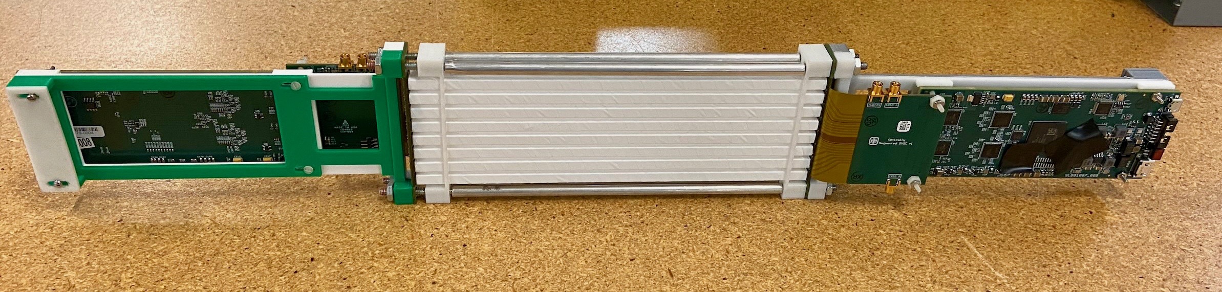
(a)

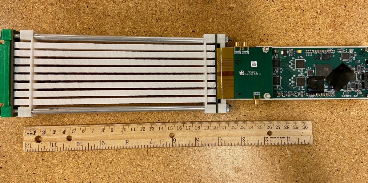
(b)

Figure 1: (a) Perspective view of a fully populated optically segmented module (OSMO), with 16 Teflon-wrapped EJ-204 bars. (b) Zoomed in photo of the OSMO for scale, lying flat on the table.

II-A Mechanical design

Each scintillator bar is wrapped with at minimum three layers of white Teflon tape. The ends of each bar are coupled to SiPMs using either EJ-560 silicone rubber optical coupling pads [19] or EJ-550 optical grease [20]; we report results for both coupling materials.

The scintillator bars are fed through 3-D printed plastic grids for support and alignment. In order to provide the pressure between the bars and the SiPMs for optimal optical coupling, we use four threaded aluminum rods. Screws pass through the plastic guides and a plastic 3-D printed support bracket. This support bracket provides the base for each of the readout boards to be rigidly connected to both the bar support guide and the threaded rods. Finally, two sets of plastic 3-D printed grids ensure that the optical pads and bars are aligned with the SiPMs and provide optical isolation between adjacent channels.

II-B Front-end electronics design and Data Acquisition

A new custom readout system was developed for the OSMO, based closely on a previous design [17]. The electronics components consist of two interconnected PCBs: the SiPM module with a $2\times 8$ SiPM array and the SCEMA waveform capture board.

The SCEMA-B PCB used for all results in this paper is based on the original SCEMA-A design [17], with modifications made to improve FPGA IO mappings, address an existing ADC problem on one channel, and to split functionality to provide a modular front-end. Whereas the SCEMA-A had a front-end that was designed to directly connect to a Planacon MCP-PMT header, the SCEMA-B includes a Samtec connector that allows for implementation of various front-ends, including a similar Planacon interface board, but also allowing for other custom readouts, such as the SiPM module described herein.

The SiPM module, shown in Fig. 2, consists of 16 SensL J-Series SiPMs (MicroFJ-60035-TSV), which have a $$6.13\text{\,}\mathrm{m}\mathrm{m}$\times$6.13\text{\,}\mathrm{m}\mathrm{m}$$ cross-section and are separated by $2\text{\,}\mathrm{m}\mathrm{m}$. A flex section allows two separate rigid PCBs to couple in an orthogonal orientation without an extra connector. The SiPM module is responsible for electrically isolating each of the 16 SiPM anodes in the array.

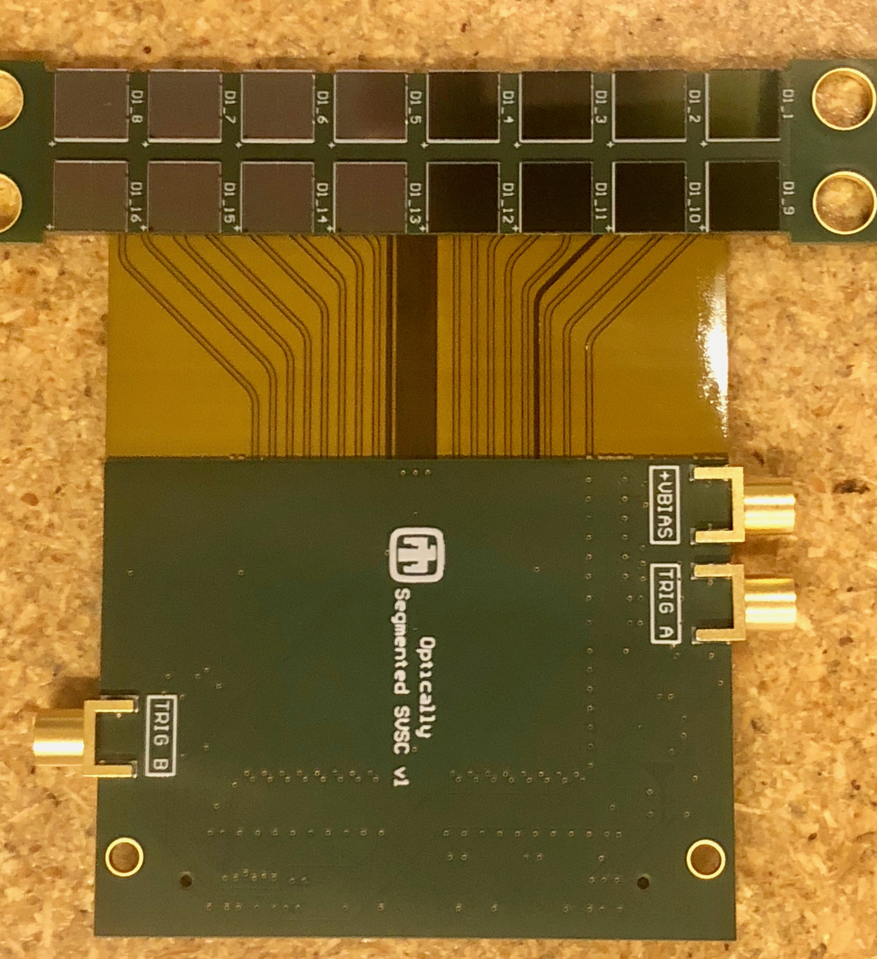
(a)

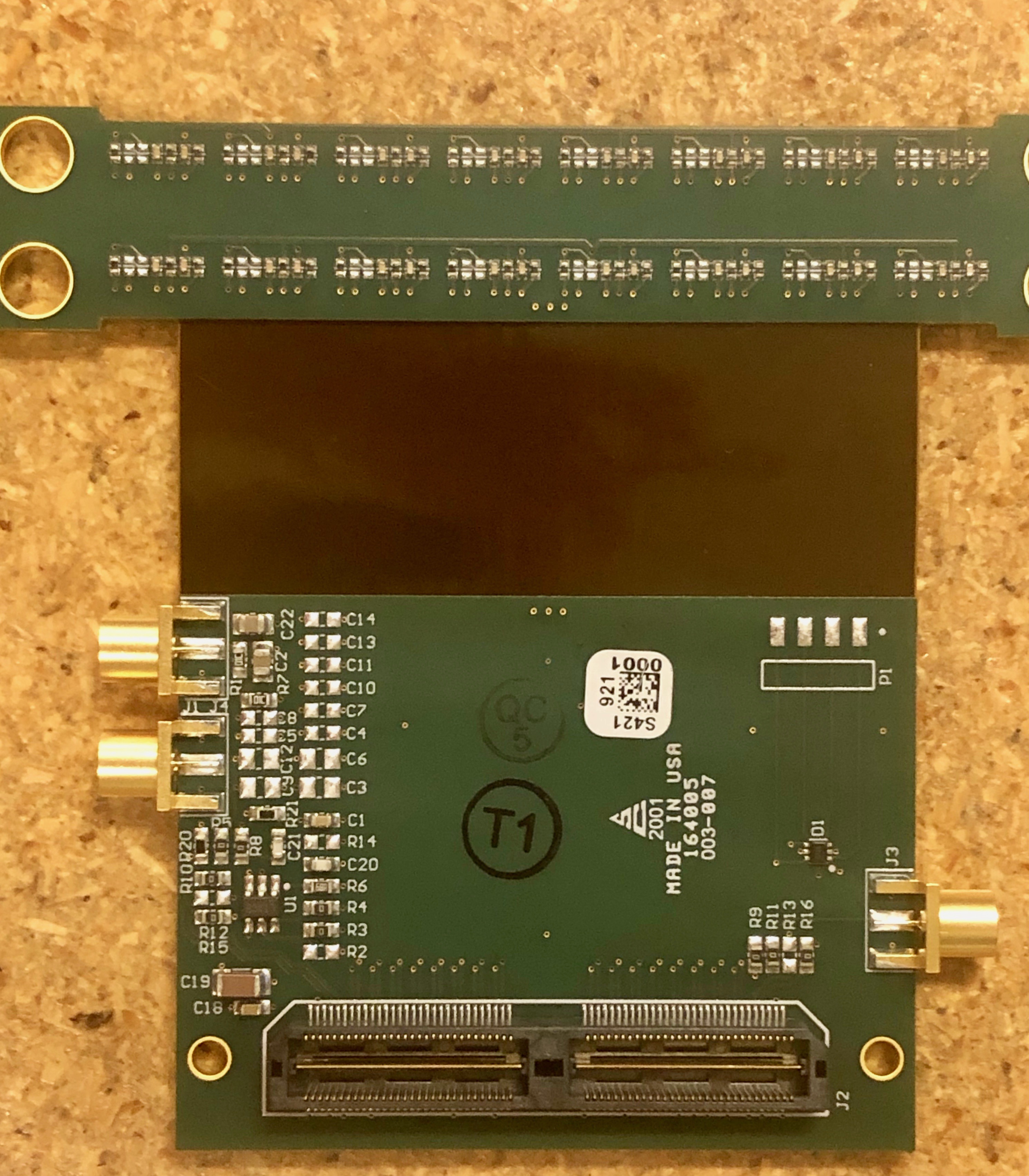
(b)

Figure 2: The top (a) and bottom (b) sides of the $2\times 8$ OSMO SiPM module board.

The SiPM module connects to the SCEMA-B via a SamTec connector (QTH-060-01-L-D-A). On each SCEMA-B are two DRS4 digitizers [21]. Each DRS4 has nine channels: eight of those channels digitize half of the SiPM array and the remaining channel is responsible for digitizing one of the trigger inputs. Thus, the SiPM module routes a total of 18 channels to the SCEMA-B: 16 SiPM channels and 2 trigger channels, which we call Trigger-A and Trigger-B.

The SiPM module also provides MCX connectors for the SiPM bias voltage, which is supplied for these studies by a B&K Precision 9129B DC power supply [22], and for the two trigger channels. Trigger-A can be configured as either an external trigger (received via the MCX connector) or as a local sum trigger, depending on whether or not a summing OpAmp is populated. This sum trigger provides self-triggering capability for one OSMO for acquiring neutron scattering data. The summing circuit reads a common-cathode signal of all 16 SiPMs and routes its output both to a DRS4 channel for digitization and to the Trigger-A MCX connector for output. Trigger-B is configured only as an external trigger; the signal from its MCX connector is simply routed to the SCEMA-B for digitization. Trigger-B is used to input the trace from the tag scintillator for the ${}^{22}\text{Na}$ calibrations described below, and can also be used to accept a trigger from the other side of the array or from the entire prototype for neutron scatter data.

The OSMO’s modular design has at least two different acquisition configurations for the SCEMA-B’s. Each SCEMA-B is able to run independently for module calibrations as well as in a connected state in a multiple OSMO system. This design allows for OSMOs to be assembled and calibrated individually, and then for multiple OSMOs to be connected together to increase the active scintillator volume of a full system. All of the data presented here was collected with each SCEMA-B running independently and with Trigger-A configured as an input trigger. The digitized data are sent from each SCEMA-B to a DAQ computer through a USB-2.0 connection, and are then written to disk. Figure 3 summarizes the DAQ configuration.

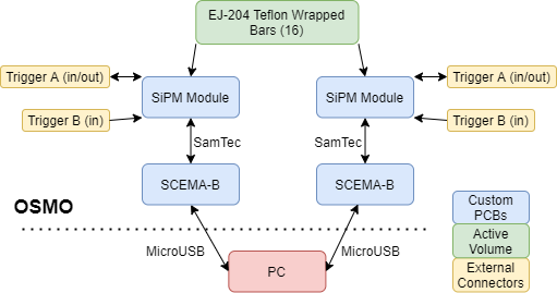
Figure 3: Diagram of the OSMO DAQ configuration.

III Module response characterization

In this section we describe the full response of a single OSMO, including electrical crosstalk on the SiPM module, SiPM module timing, and scintillator interaction response calibrations for the energy, position, and time. Results are presented for two scintillator/SiPM coupling materials: EJ-550 optical grease and $0.5\text{\,}\mathrm{m}\mathrm{m}$ thick EJ-560 silicone rubber pads.

III-A Waveform analysis

Digitized waveforms from the SCEMA-B boards are analyzed with custom C++-based software utilizing ROOT libraries [23]. The values of interest are the rising edge time of the trigger channels, the rising edge time of the SiPM traces, and the maximum pulse height for each SiPM waveform. The DRS4s are sampled at $\approx$$4.9\text{\,}\mathrm{G}\mathrm{H}\mathrm{z}$, and all 1024 bins within the switched capacitor array (SCA) are digitized for each triggered event. Electrical calibrations for timing and voltage are calculated using a similar procedure to that reported previously [17].

It was also observed that there is some time dependent drift in the voltage calibration for each of the bins within the DRS4 SCA. In order to account for the voltage drift before each run, we subtract from each voltage bin the mean average of the voltage of the same bin within the SCA. Before additional processing but after DRS4 electrical calibrations, baseline offsets for the entire waveform are calculated as the mean of the samples 20 through 60 of each waveform. After this procedure we obtain a voltage baseline deviation of $\approx 1.0\text{\,}\mathrm{\SIUnitSymbolMicro}\mathrm{V}$, and voltage noise between $0.3\text{\,}\mathrm{m}\mathrm{V}0.5\text{\,}\mathrm{m}\mathrm{V}$.

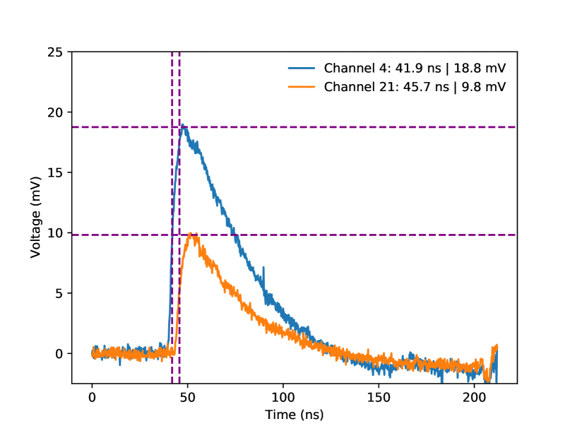
Figure 4: An example bar interaction from a ${}^{22}\text{Na}$ source with digitized waveforms for the two SiPMs coupled to the ends of one bar. The vertical lines represent where the analysis identifies the half-point rising edge of the waveform. The horizontal lines indicate the value the analysis identifies as the pulse height of the waveform.

Pulse heights of each SiPM trace are measured based on the following algorithm. We first determine the six consecutive samples that give the largest integrated value. We discard the highest and lowest of these six values and report the average of the four remaining values as the pulse height. By dropping the highest and lowest bin voltage values, we avoid noise that appears in some DRS4 bins, which (when present) was always separated by 32 bins and could not be resolved with voltage calibrations alone.

Rise time measurements are determined from the interpolated value between the samples corresponding to $50\text{\,}\mathrm{\char 37\relax}$ of the measured pulse height previously discussed. Figure 4 shows the traces from both SiPMs for an example bar interaction. The measured pulse heights and rise times for both traces are indicated by vertical and horizontal dashed lines.

III-B Electrical crosstalk characterization

One motivation for a custom SiPM array was to reduce electrical crosstalk between SiPM channels compared to the commercial J-series array [24]. To characterize the electrical crosstalk of the system, we used a Photek LPG-405 laser [25] as a known input source on each of the 16 individual SiPM channels, as shown in Fig. 5. The laser was triggered externally using a digital delay and pulse generator from Stanford Research Systems (DG535), which was set to a nominal trigger rate of $50\text{\,}\mathrm{H}\mathrm{z}$, approximately the maximum trigger rate for a single SCEMA in this setup. After the DG535 sends a trigger to the laser, the laser then sends a trigger signal to Trigger-B, the independent board trigger, followed $\approx$ $47\text{\,}\mathrm{n}\mathrm{s}$ later by an incident photon packet. The resulting waveforms for all channels are then recorded. All electrical crosstalk results are presented with the summing circuit populated.

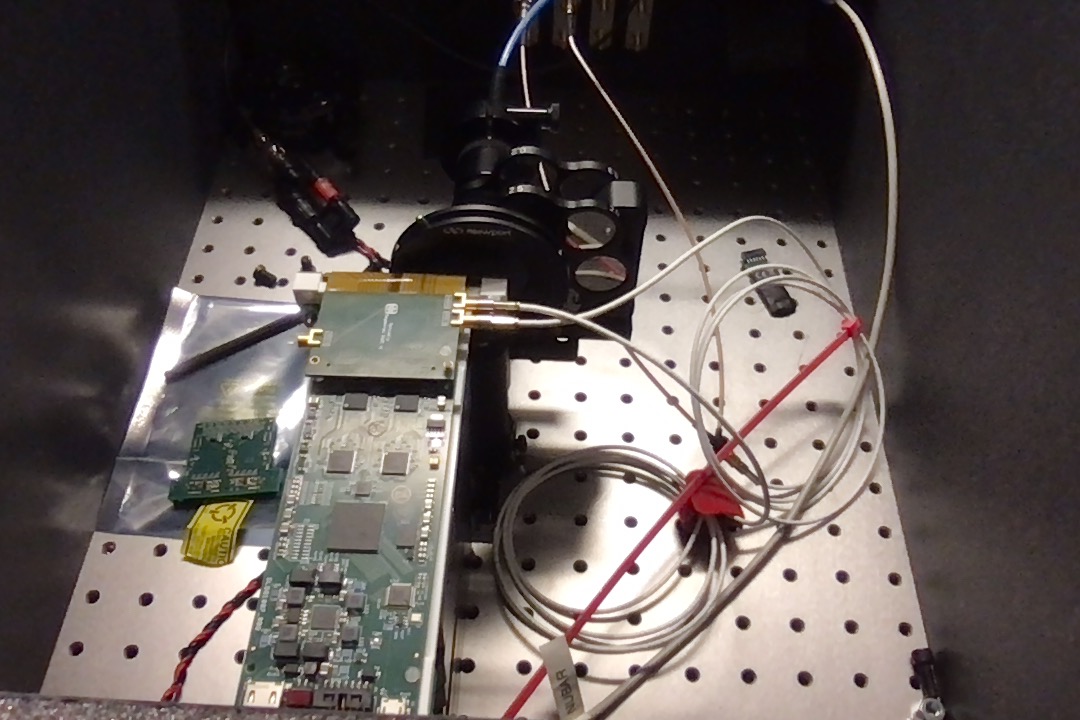
(a)

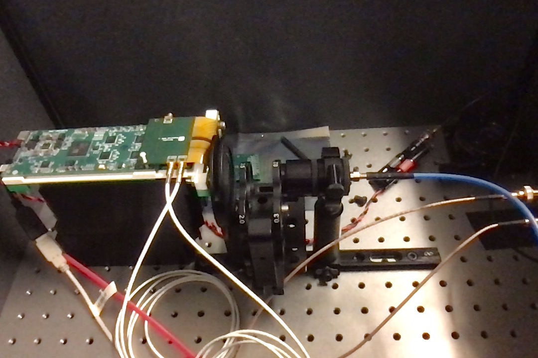
(b)

Figure 5: (a) Image of the laser setup from behind. The whole SCEMA is aligned to the stationary optical shield to expose a single pixel to the laser. (b) Image of the laser test-setup from the side. The blue cable is an optical fiber which directs the output laser packet. An optical shield and filter are used to isolate a single pixel as the target pixel for the run. The variable optical attenuator is used to tune the SiPM response to the laser.

We measure the amount of electrical crosstalk between a target channel and remaining channels using both the coincident measured pulse height and the total pulse integral of the target channel and the other 15 channels. The pulse height measured for the remaining channels is the measured pulse height using the algorithm defined in Section III-A where the measured pulse height must happen after $2\text{\,}\mathrm{n}\mathrm{s}$ before the rising-edge of the target channel’s response. This ensures that the appropriate region of interest is measured. Similarly, the waveform integral is calculated for all waveforms beginning $2\text{\,}\mathrm{n}\mathrm{s}$ before the measured rising edge of the target channel.

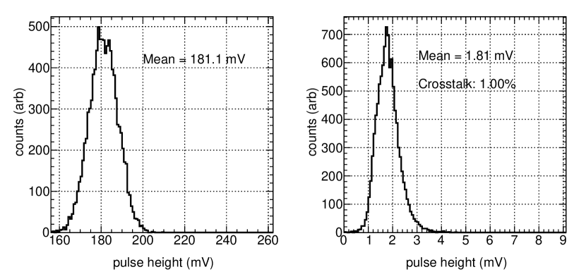
Figure 6: Example pulse height measurement comparing the distribution of the target channel (left) and an adjacent channel (right).

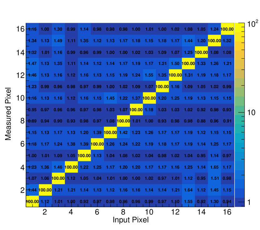
(a)

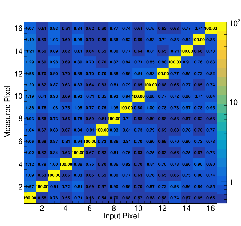
(b)

Figure 7: (a) Crosstalk Integral Calculation. (b) Crosstalk Pulse Height Calculation.

The crosstalk percentage for both the pulse height and total integral is defined as the mean average of each channel’s response divided by the mean average of the target channel’s response. A series of 10k events are recorded when the laser is targeted at a single input pixel. Two example pulse height distributions for one target pixel position are shown in Fig. 6. This procedure is performed using all 16 channels within the array as the target pixel; the results for both pulse height and waveform integral are shown in Fig. 7

The input pixel in Fig. 7 is defined as the target pixel of the laser. Both integral and pulse height measurements are compared as a relative percentage of the input pixel. Target channels 2, 4, 6, 7, 10, 12, 13, and 15 all correspond to one (1$\times$8) column within the SiPM module.

We find that the total crosstalk among channels is $\approx$ 1% or less even with relatively large input pulses ($\approx$ $200\text{\,}\mathrm{m}\mathrm{V}$) on target channels. Fig. 8 shows the pulse height crosstalk measurement for all channels. The horizontal line is a 0th-order polynomial fit to all data, indicating an average crosstalk of 0.76% for the SiPM module. Since pulse heights used in detector calibration are in the range $15\text{\,}\mathrm{m}\mathrm{V}30\text{\,}\mathrm{m}\mathrm{V}$, a $1\text{\,}\mathrm{\char 37\relax}$ crosstalk would imply a pulse height (from only electrical crosstalk) of $150\text{\,}\mathrm{\SIUnitSymbolMicro}\mathrm{V}300\text{\,}\mathrm{\SIUnitSymbolMicro}\mathrm{V}$. This value is within the measured electrical noise ($\approx 0.5\text{\,}\mathrm{m}\mathrm{V}$), and we therefore do not expect electrical crosstalk to significantly impact our results.

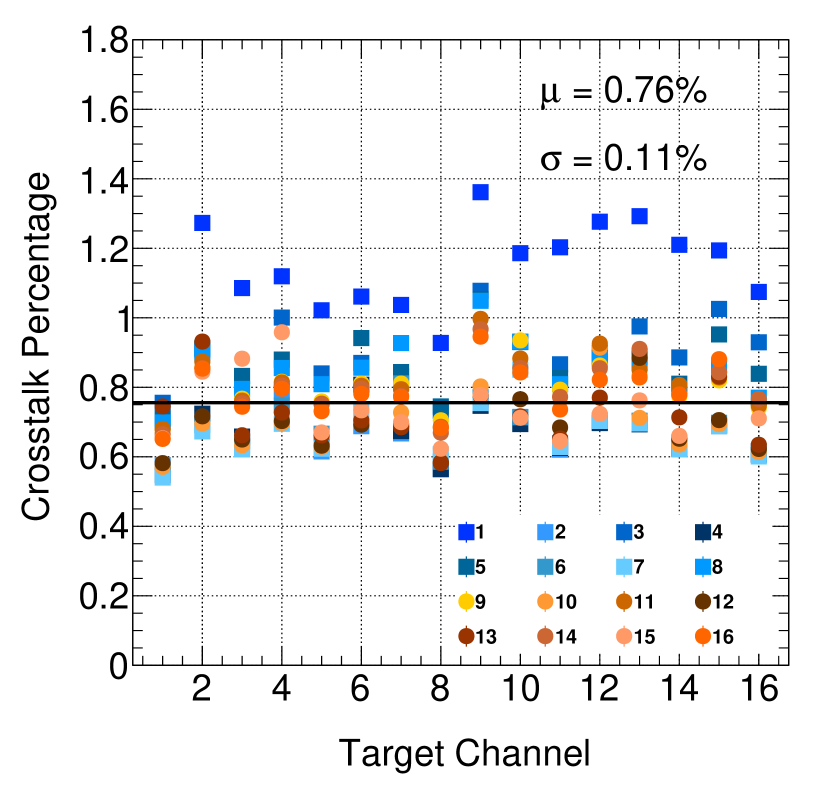
Figure 8: Distribution of all of the crosstalk in percentages for pulse height. For the zeroth-order fit, we ignore the crosstalk contributions from channel 1, since channel 1 had a known electrical calibration error which skews the results. Statistical error bars are too small to see on the plot.

III-C SiPM timing response

Additional laser studies were performed to characterize the timing resolution as a function of measured pulse height. In order to vary the laser intensity on the SiPM, an variable optical attenuator (shown on right image of Fig. 5) was used. Similar to the electrical crosstalk measurements, laser pulses are sent at a rate of $50\text{\,}\mathrm{H}\mathrm{z}$ to the SCEMA-B, preceded by a trigger from the DG-535. The time resolution is then defined as the standard deviation from a Gaussian fit to the time difference measured between the arrival time of the input trigger and the rise-time of the pulse height.

Fig. 9 shows the the approximate timing uncertainty for an example channel as a function of voltage response from the SiPM due to the laser input. Each point represents time differences with pulse height values measured within $25\text{\,}\mathrm{m}\mathrm{V}$ of the plotted point. We find that, as the pulse height increases, the timing resolution improves asymptotically to $\approx 80\text{\,}\mathrm{p}\mathrm{s}$. Since the reported timing jitter between the laser’s trigger and pulse is much less ($T_{sl}=$2\text{\,}\mathrm{p}\mathrm{s}$$ [25]), we find that most of the timing uncertainty is due to the pulse height and readout electronics.

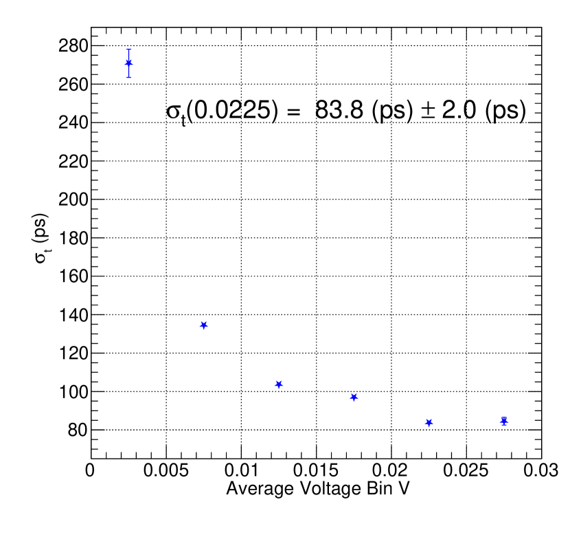
Figure 9: Example timing resolution of a single SiPM as a function of measured SiPM pulse height. A Photek laser with an optical attenuator is used as an input to a SiPM. The timing resolution is sigma of a Gaussian fit to the difference in time between the trigger and the pulse height. The error bars presented are statistical from the Gaussian fits.

The timing resolution values for small voltages ($<$ $5\text{\,}\mathrm{m}\mathrm{V}$) have large values and indicate that the SiPM’s rise-time compared to noise is not well measured. Larger values for the SiPM response were not measured since pulses greater than $\approx$ $30\text{\,}\mathrm{m}\mathrm{V}$ are not used in the calibration procedure described below.

III-D Interaction calibration setup

The bar calibration procedure involves a single ${}^{22}\text{Na}$ source. We use the simultaneous and back-to-back $0.511\text{\,}\mathrm{M}\mathrm{e}\mathrm{V}$ gammas using a procedure similar to methods in both [11] and [15]. The tag scintillator is a teflon-wrapped stilbene crystal that is $5.0\text{\,}\mathrm{c}\mathrm{m}$ in height and has a $0.5\text{\,}\mathrm{c}\mathrm{m}$ $\times$ $0.5\text{\,}\mathrm{c}\mathrm{m}$ cross section. The tag scintillator rests on top of the J-series SensL eval board SiPM and is optically coupled using EJ-550 optical grease.

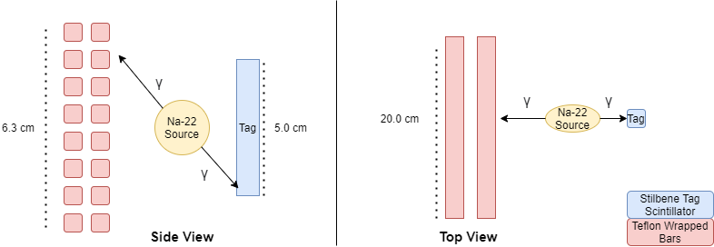
Figure 10: Setup of the ${}^{22}\text{Na}$ tag scintillator and OSMO.

Since the crystal’s height is approximately $2.0\text{\,}\mathrm{c}\mathrm{m}$ smaller than total span of the eight scintillator bars, the ${}^{22}\text{Na}$ source is placed closer to the tag to create a magnification effect so that all of the bars can be targeted by the range of particles hitting the tag, as shown in Fig. 10. The use of a larger scintillator tag with magnification allows a single scan across the length of the OSMO to target the bars in half of the matrix. In order to precisely move the ${}^{22}\text{Na}$ source and tag along the length of the OSMO, we use the eTrack $250\text{\,}\mathrm{m}\mathrm{m}$ linear stage with NEMA 17 MDrive motor from Newmark Systems, which is controlled via the host computer for data acquisition through a USB to RS422 converter. A picture of the experimental setup is shown in Fig. 11.

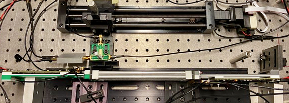
Figure 11: Top-down view of the ${}^{22}\text{Na}$ calibration scan procedure is shown. The SensL eval board and tag are on the top of the image, with the ${}^{22}\text{Na}$ source holder between it and the OSMO.

The two independent SCEMA-B boards are powered by a B&K Precision 9129B DC power supply, which provides two independent channels of $5.6\text{\,}\mathrm{V}\mathrm{D}\mathrm{C}$ power, and are connected to a control computer via micro-USB through a USB hub. The SiPMs are provided a $30\text{\,}\mathrm{V}$ bias, or an approximate $6\text{\,}\mathrm{V}$ over-voltage, supplied by a B&K Precision 1761 power supply. Additionally, $30\text{\,}\mathrm{V}\mathrm{D}\mathrm{C}$ is supplied to a single SensL J-series eval board which is used to read out the tag scintillator. We use both the standard and fast outputs from the eval board. The standard output is sent to a Photek PA200-10 (Mini-Circuits ZFL-1000LN+) $20\text{\,}\mathrm{d}\mathrm{B}$ amplifier, which is routed to the DG535 pulse generator as the system trigger.

We set a $0.18\text{\,}\mathrm{V}$ input trigger threshold on the DG535. When the threshold is exceeded, the DG535 issues two parallel triggers ($200\text{\,}\mathrm{m}\mathrm{V}$ step function) with $5\text{\,}\mathrm{p}\mathrm{s}$ jitter [26] to the Trigger-A of each SCEMA-B. The fast output from the eval board is sent to the Trigger-B of one SCEMA-B in order to digitize the fast-output spectrum from the tag and thus measure both an absolute reference time for the interaction and the tag’s ${}^{22}\text{Na}$ pulse height spectrum.

III-E Interaction energy response

The energy spectrum for each bar is fit in the range of $0.225\text{\,}\mathrm{M}\mathrm{e}\mathrm{V}0.4\text{\,}\mathrm{M}\mathrm{e}\mathrm{V}$ to the predicted Klein-Nishina spectrum for back-to-back $0.511\text{\,}\mathrm{M}\mathrm{e}\mathrm{V}$ gammas using the method described in [15]. This energy calibration is performed for the two photodetectors coupled to the ends of each bar; an example is shown in Fig. 12. The resulting scaling factors for each of the photodetectors is used to convert measured pulse height in mV to an energy in MeVee.

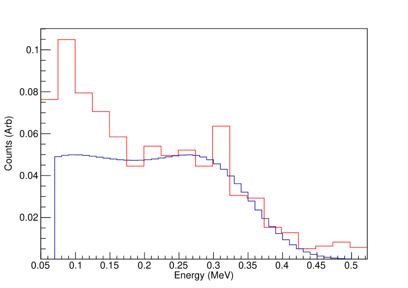
(a)

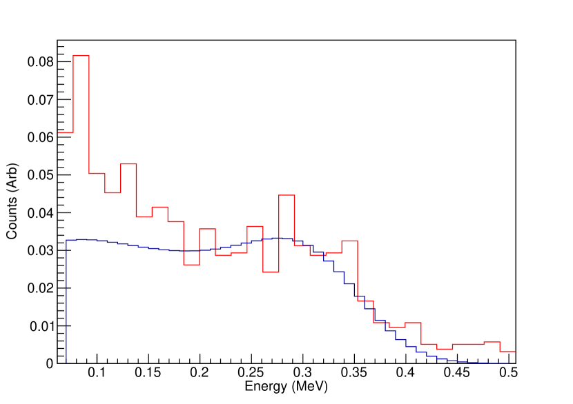
(b)

Figure 12: Example of an energy calibration for a single bar. The red and blue histograms represent data and the fit respectively. The region of interest for the Klein-Nishina fit is $0.225\text{\,}\mathrm{M}\mathrm{e}\mathrm{V}\mathrm{e}\mathrm{e}0.4\text{\,}\mathrm{M}\mathrm{e}\mathrm{V}\mathrm{e}\mathrm{e}$. (a)/(b) Shows the fit to the Klein-Nishina prediction for the two photodetectors on each bar end.

In the following sections we present the position and time resolution of the bars for events within different energy ranges and fit the results to a power law. We quote the position and time resolution energy ranges from $0.0\text{\,}\mathrm{M}\mathrm{e}\mathrm{V}\mathrm{e}\mathrm{e}0.4\text{\,}\mathrm{M}\mathrm{e}\mathrm{V}\mathrm{e}\mathrm{e}$ in steps of $0.10\text{\,}\mathrm{M}\mathrm{e}\mathrm{V}\mathrm{e}\mathrm{e}$, which fully covers the Compton spectrum resulting from $0.511\text{\,}\mathrm{M}\mathrm{e}\mathrm{V}\mathrm{e}\mathrm{e}$ gammas from the ${}^{22}\text{Na}$ source.

III-F Interaction position resolution

The interaction position along a bar is determined using both the difference in rising edge time between the two readout SiPMs for each bar and their relative pulse heights. We combine the measurements using the Best-Linear-Unbiased-Estimator (BLUE) [27] to obtain an overall position resolution.

The interaction position using SiPM pulse heights from each bar is determined by the log of the amplitude ratio (LAR) between the two bar ends, or $\ln\frac{A_{1}}{A_{2}}$, where $A_{1}$ and $A_{2}$ are the pulse heights measured from the output SiPMs from the end of each bar. The mean LAR as a function of interaction position for Bar 1 in the $0.3\text{\,}\mathrm{M}\mathrm{e}\mathrm{V}\mathrm{e}\mathrm{e}0.4\text{\,}\mathrm{M}\mathrm{e}\mathrm{V}\mathrm{e}\mathrm{e}$ range, measured with a Gaussian fit to the distribution, is shown in Fig. 13a. The standard deviation of the distribution as a function of interaction position is shown in Fig. 13b. The reported position resolution for this bar, which was coupled with optical grease to the SiPM, is the average LAR width divided by the slope of the LAR means, or $1.8\text{\,}\mathrm{c}\mathrm{m}$. Fig. 14 shows the LAR as a function of interaction position for all 16 bars coupled with optical grease coupling.

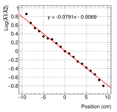
(a)

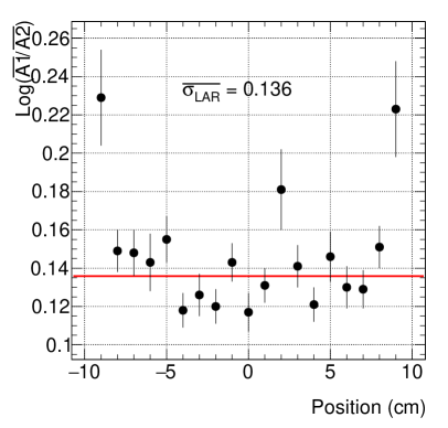
(b)

Figure 13: Example dependence of the mean LAR as a function of source position for Bar 1 in the OSMO. After energy calibrations to determine the MeVee/mV ratio for each bar, a cut is performed to filter only events in the $0.3\text{\,}\mathrm{M}\mathrm{e}\mathrm{V}\mathrm{e}\mathrm{e}0.4\text{\,}\mathrm{M}\mathrm{e}\mathrm{V}\mathrm{e}\mathrm{e}$ range. Then the LAR is calculated and a Gaussian fit is performed for each source position. Data points and uncertainties in (a) are the Gaussian mean and uncertainties reported from the (ROOT default) fitting algorithm. In (a), error bars are smaller than the markers. Data points and uncertainties in (b) are the fitted Gaussian sigma and the uncertainties reported from the fitting algorithm.

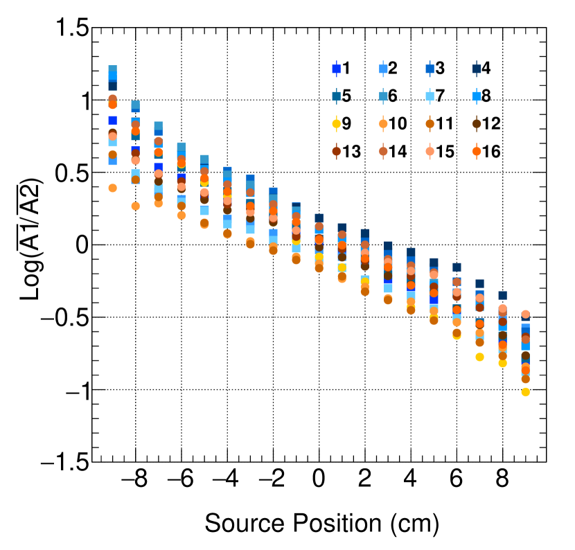
Figure 14: The mean LAR for all of the bars as a function of the interaction position.

In previous studies [11, 15], the position resolution using timing was computed by taking the difference of the pulse rise times of each SiPM from the end of each bar: $t_{1}-t_{2}$. However, in this case the time measurements on a single OSMO are measured using two different SCEMA-Bs. In these measurements, the two SCEMA-Bs and their corresponding DRS4s run asynchronously. We therefore use the time of the synchronized trigger pulse from the DG-535 into the Trigger-A inputs ($T^{A}_{1,2}$) in order to align the timing between SCEMAs:

$$~{}\Delta{t}=(T^{A}_{1}-t_{1})-(T^{A}_{2}-t_{2})$$ (3)

From the above equation, we substitute $T_{i}=T^{A}_{i}-t_{i}$ to identify the relative time difference measured on each SCEMA and obtain equation:

$$~{}\Delta{t}=T_{1}-T_{2}$$ (4)

Fig. 15 shows the mean and standard deviation of the time difference distributions as function of interaction position for Bar 1 coupled with optical grease, again in the $0.3\text{\,}\mathrm{M}\mathrm{e}\mathrm{V}\mathrm{e}\mathrm{e}0.4\text{\,}\mathrm{M}\mathrm{e}\mathrm{V}\mathrm{e}\mathrm{e}$ range. The position resolution using time difference for this bar is $2.08\text{\,}\mathrm{c}\mathrm{m}$. Fig. 16 shows the mean of time difference for all 16 bars with optical grease coupling: the two different y-intercept distributions correspond to the two different DRS4 pairs on each SCEMA-B, resulting in distinct timing offsets. The bottom 8 bars correspond to when a bar’s SiPM channels are read by the same DRS4 as the trigger channel, and the top 8 bars’ SiPM channels are digitized by the other DRS4. The combined BLUE position resolution as a function of energy is shown in Fig. 17, in which the mean position resolution for all 16 bars is used.

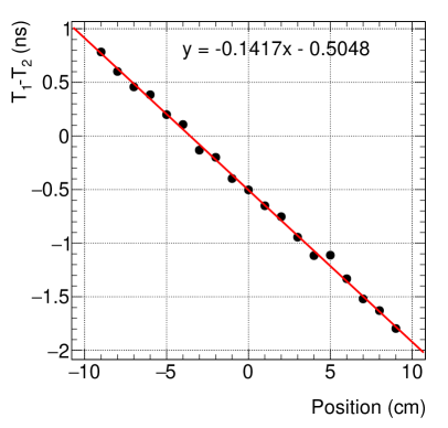
(a)

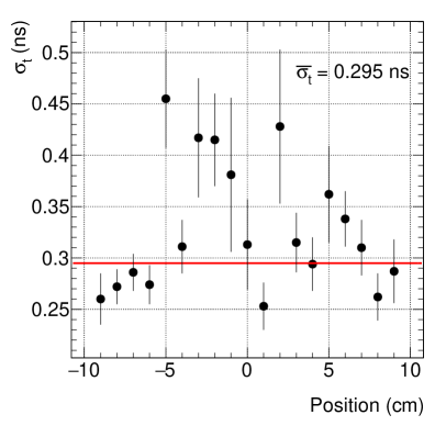
(b)

Figure 15: Example dependence of the time difference as a function of source position for Bar 1 in the OSMO. After energy calibrations to determine the MeVee/mV ratio for each bar, a cut is performed to filter only events in the $0.3\text{\,}\mathrm{M}\mathrm{e}\mathrm{V}\mathrm{e}\mathrm{e}0.4\text{\,}\mathrm{M}\mathrm{e}\mathrm{V}\mathrm{e}\mathrm{e}$ range. Then the time difference is calculated and a Gaussian fit is performed for each source position. Data points and uncertainties in (a) are the Gaussian mean and uncertainties reported from the (ROOT default) fitting algorithm. In (a), error bars are smaller than the markers. Data points and uncertainties in (b) are the fitted Gaussian sigma and the uncertainties reported from the fitting algorithm.

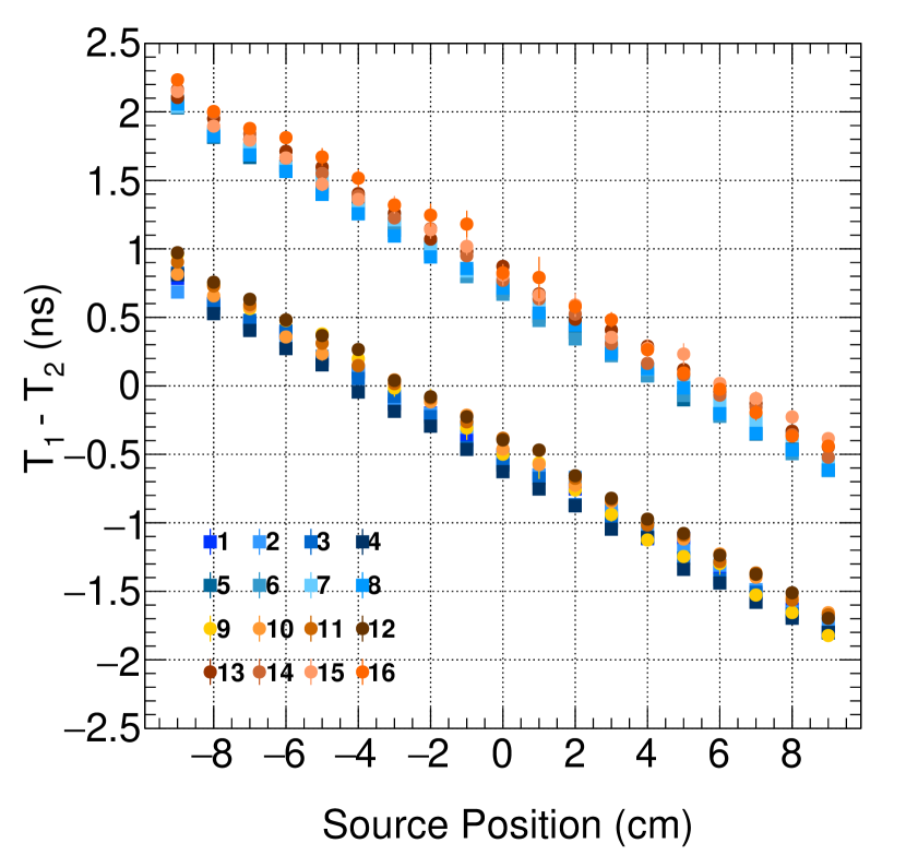
Figure 16: The results of a Gaussian fit to the time difference for all bars at different ${}^{22}\text{Na}$ scan positions. The points represent the means and the error bars are the sigma from the fit. The two different y-intercept distributions correspond to bars digitized by the same DRS4 as the trigger channel (bottom group) and other DRS4 (top group), and represent the timing offset between the two DRS4s.

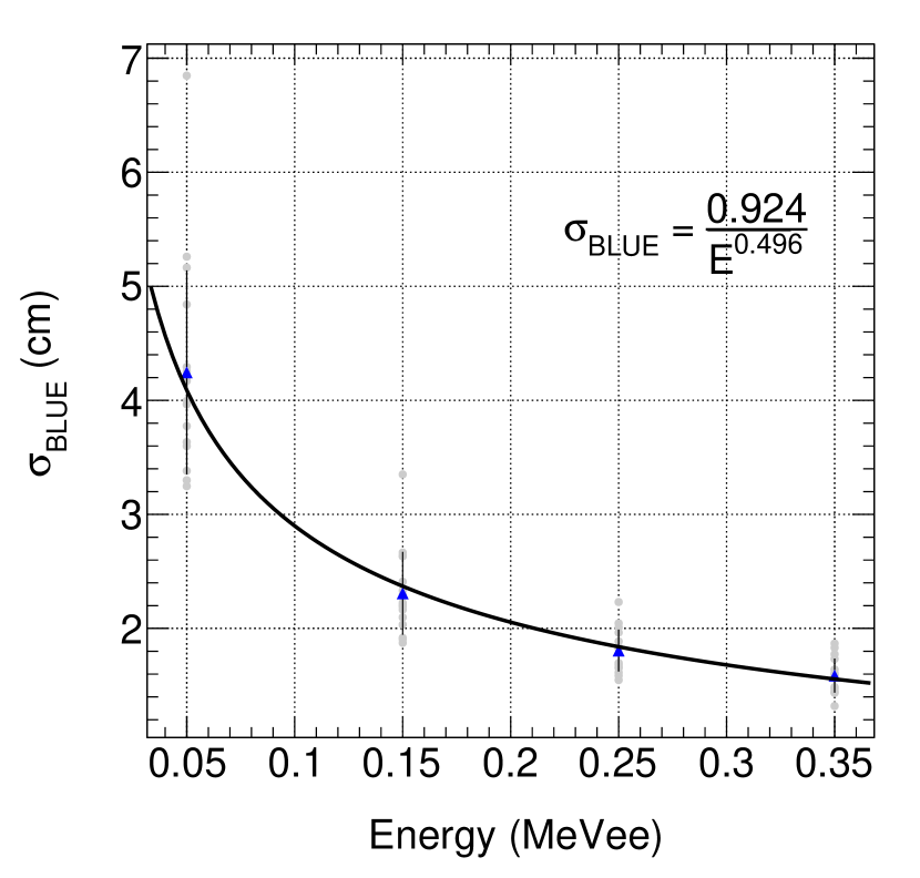
Figure 17: The average position resolution for each bar as a function of energy is fit to a power law. Each point’s value along the x-axis represents the mean value of the range. The grey points indicate the results for the 16 bars in the OSMO. The blue points indicate the mean of the 16 bars. The error bars on the mean data points represent the standard deviation of the mean of the 16 bars. The fit is then applied to the blue points.

III-G Interaction time response

The interaction time is defined as the average of the pulse rise times for each bar end minus the rise time of the tag pulse ($t_{1}^{B}$), which is used as an absolute time reference. As before, the rise time of each bar end has a correction from the Trigger-A input to correct for the asynchronous SCEMA acquisition, including the tag’s rise time input to Trigger-B:

$$~{}T_{int}=\frac{(T_{1}^{A}-t_{1})+(T_{2}^{A}-t_{2})}{2}-(T_{1}^{A}-t_{1}^{B})$$ (5)

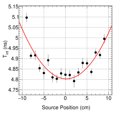
(a)

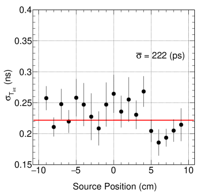
(b)

Figure 18: (a) Interaction time is shown for an example bar (Bar1), in the module. We expect a symmetrical effect about the bar length, for any given positional dependence of the interaction time. (b) The average uncertainty in the interaction time for Bar 1 at each of the scan positions. We fit a zeroth order polynomial to find an average uncertainty for each bar.

The mean and standard deviation of the interaction time distributions as a function of interaction position for Bar 1 coupled with optical grease are shown in Fig. 18: the reported interaction resolution is 248 ps for this bar. It has been previously observed that interaction time within a bar has a positional dependence along a bar’s length [15], which is again observed here. The energy-dependent average interaction time resolution is shown in Fig. 19. The offset from the interaction time in Fig. 18 occurs from the minimum average delay time from equation (5).

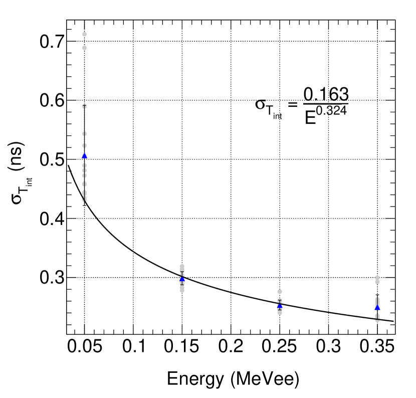
Figure 19: The average interaction time for each bar is fit to a power law. The grey points indicate the results for the 16 bars in the OSMO. The blue points indicate the mean of the 16 bars. The error bars on the mean data points represent the standard deviation of the mean of the 16 bars. The fit is then applied to the blue points.

IV Summary of results and discussion

Here we present position and interaction time resolution results for all 16 channels in the assembled OSMO. Tables I and II summarize the position and timing resolutions for EJ-550 and EJ-560 optical coupling material, respectively. In the last two rows, we report the mean and standard deviation of the given resolution across the 16 bars. We note that overall, the EJ-550 optical coupling has improved position and timing resolution values compared to EJ-560. However, there are some bars for which the EJ-560 silicone pads have better position resolution than with optical grease. Compared to the EJ-550 data, resolution values are noticeably better for bars {2,7,15}, which are close to the tightening screws of the OSMO.

TABLE I: Resolution Results with EJ-550 optical grease coupling.

Bar ID	$\sigma_{z}^{t}$ (cm)	$\sigma_{z}^{A}$ (cm)	$\sigma_{z}$ (cm)	$\sigma_{\text{int}}$ (ps)
1	2.08	1.72	1.34	222
2	2.44	2.76	1.83	244
3	1.94	1.71	1.29	242
4	1.95	2.11	1.43	233
5	1.91	1.79	1.31	226
6	1.93	1.65	1.26	227
7	2.22	2.16	1.55	228
8	2.06	1.85	1.38	231
9	1.78	1.52	1.16	234
10	2.32	2.68	1.76	247
11	2.06	2.07	1.46	229
12	1.99	2.13	1.46	239
13	2.13	2.16	1.52	224
14	2.18	1.95	1.46	238
15	2.53	2.54	1.79	263
16	1.98	1.56	1.24	240
$\bar{x}$	2.09	2.02	1.45	235
$\sigma_{\text{std}}$	0.20	0.37	0.19	10

TABLE II: Resolution Results with EJ-560 silicone pads for coupling.

Bar ID	$\sigma_{z}^{t}$ (cm)	$\sigma_{z}^{A}$ (cm)	$\sigma_{z}$ (cm)	$\sigma_{\text{int}}$ (ps)
1	2.41	2.19	1.62	253
2	2.13	2.42	1.61	244
3	3.00	4.81	2.70	258
4	2.83	4.33	2.48	264
5	2.99	4.95	2.73	262
6	2.60	3.55	2.15	297
7	2.04	1.76	1.34	238
8	2.02	1.88	1.38	248
9	2.29	2.20	1.59	263
10	7.45	9.28	5.90	352
11	2.82	3.16	2.11	264
12	3.53	6.47	3.41	300
13	3.04	2.49	1.95	280
14	2.75	2.57	1.88	250
15	2.16	1.96	1.45	237
16	2.18	2.05	1.50	236
$\bar{x}$	2.89	3.50	2.24	265
$\sigma_{\text{std}}$	1.25	1.99	1.10	29

The bars where EJ-560 has improved $\sigma_{\text{blue}}$ resolution compared to EJ-550 are bars 2, 7, and 15. All three of these bars are also close to the tightening screws on the OSMO. One possibility is that these bars have better optical coupling between the scintillator and SiPM in the optical pad configuration due to better compression or alignment, and therefore the SiPMs collected more light. Figure 20 highlights the differences in position resolution between the two optical-coupling configurations.

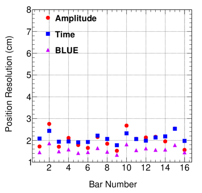
(a) EJ-550 optical grease

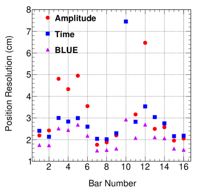
(b) EJ-560 silicone pads

Figure 20: (a) A graphical representation of Table I. (b) A graphical representation of Table II.

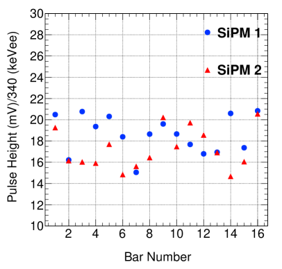
(a) EJ-550 optical grease

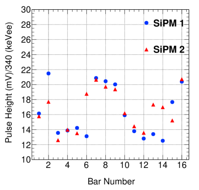
(b) EJ-560 silicone pads

Figure 21: (a) Pulse height response in mV to a $340\text{\,}\mathrm{k}\mathrm{e}\mathrm{V}\mathrm{e}\mathrm{e}$ gamma interaction using the EJ-550 optical grease dataset. (b) Pulse height response in mV to a $340\text{\,}\mathrm{k}\mathrm{e}\mathrm{V}\mathrm{e}\mathrm{e}$ gamma interaction using the EJ-560 silicone pad dataset.

We observe the average and standard deviation of position resolution for the 16 bars coupled with EJ-550 to be $$1.45\text{\,}\mathrm{c}\mathrm{m}$\pm$0.19\text{\,}\mathrm{c}\mathrm{m}$$ and with EJ-560 to be $$2.24\text{\,}\mathrm{c}\mathrm{m}$\pm$1.10\text{\,}\mathrm{c}\mathrm{m}$$. We also observe an average and standard deviation of the interaction time resolution for the 16 bars with EJ-550 to be $$235\text{\,}\mathrm{p}\mathrm{s}$\pm$10\text{\,}\mathrm{p}\mathrm{s}$$ and with EJ-560 to be $$265\text{\,}\mathrm{p}\mathrm{s}$\pm$29\text{\,}\mathrm{p}\mathrm{s}$$. We note that bar number 10 had substantially different position resolution with the EJ-560 coupling, which we also attribute to poor light collection of the optical pad.

One source of the difference in overall position and interaction time resolutions between to the two configurations is the amount of light collected at the ends of the SiPMs. Figure 21 highlights the differences in the results of the energy calibrations for each of the photodetectors for each bar. The energy calibration results show the amplitude response (in mV) calculated for the Compton edge of the ${}^{22}\text{Na}$ source. A decreased amplitude response corresponds to an overall decrease in the light collected by the SiPM. A decrease in the amplitude response from a SiPM directly affects both the timing resolution by affecting SiPM’s response time (Fig. 9) and amplitude resolution by reducing the signal-to-noise ratio of the measured pulse. Therefore, a decrease in the amount of light collected (a lower amplitude response) will negatively affect both interaction time and position reconstruction.

Another source of timing uncertainty is the use of multiple DRS4s which share independent clocks between the two unsynchronized SCEMA-Bs. Previous studies [15] relied on digitization chains that used channels all on a single synchronized DRS4. Another potential source of additional timing uncertainty is the use of $20\text{\,}\mathrm{c}\mathrm{m}$ long EJ-204 scintillator bars in this study compared to $19\text{\,}\mathrm{c}\mathrm{m}$ as in previous studies.

Compared to previous results [15], we observe an increase in combined position reconstruction uncertainty from $\approx 1.0\text{\,}\mathrm{c}\mathrm{m}$ to $\approx 1.45\text{\,}\mathrm{c}\mathrm{m}$. Additionally, we observe that the interaction time uncertainty has increased from $$154\text{\,}\mathrm{p}\mathrm{s}$\pm$3\text{\,}\mathrm{p}\mathrm{s}$$ to $$235\text{\,}\mathrm{p}\mathrm{s}$\pm$10\text{\,}\mathrm{p}\mathrm{s}$$. Position reconstruction and interaction time resolution could be improved both with increased light detected by a SiPM and in an OSMO where both SCEMAs are controlled synchronously, which allows all DRS4s to operate with a common clock. Syncrhonized SCEMA-Bs would eliminate the need to measure $T^{A}_{1,2}$ and remove the substitution required in (3) and (5).

V Conclusions

We designed, assembled, and characterized a modular SiPM-based scintillator array. We also compared detector calibration results for a single module using both EJ-560 and EJ-550 as optical couplings. We find that, on average, EJ-550 optical grease outperforms the EJ-560 silicone pads, which we attribute to improved light collection by each SiPM due to improved optical coupling. We therefore find that a major factor affecting an OSMO’s position reconstruction and interaction time resolutions are the variable optical couplings among the 16 bars. Since the optical coupling affects the amount of light collected by the SiPM, it also affects the SiPM’s timing response which directly affects both the interaction time uncertainty and the position reconstruction uncertainty.

We suspect improved interaction time resolutions and position reconstruction would result both from better optical coupling and with synchronized SCEMA-Bs. Finally, we note that SiPM electronic readout and scintillator differences relative to [15] may have also contributed to the differences in both measured position reconstruction and interaction time resolutions. Plans for future work include calibrating additional OSMOs, and to combine multiple-synchronized OSMOs together into a fully realized neutron imaging system. Current neutron-imaging tests are being performed using the single calibrated module presented here with the EJ-550 optical grease for coupling.

References

-
[1]
J. Manfredi, E. Adamek, J. A. Brown, E. Brubaker, B. Cabrera-Palmer, J. W.
Cates, R. Dorrill, A. Druetzler, J. Elam, P. L. Feng, M. Folsom,
A. Galindo-Tellez, B. L. Goldblum, P. Hausladen, N. Kaneshige, K. Keefe,
T. A. Laplace, J. Learned, A. Mane, P. Marleau, J. Mattingly, M. Mishra,
A. Moustafa, J. Nattress, K. Nishimura, J. Steele, M. Sweany, K. Weinfurther,
K.-P. Ziock, The single-volume
scatter camera, in: M. Fiederle, A. Burger, S. A. Payne (Eds.), Hard X-Ray,
Gamma-Ray, and Neutron Detector Physics XXII, SPIE, 2020, p. 114940V.
doi:10.1117/12.2569995.
URL https://doi.org/10.1117/12.2569995 -
[2]
W. C. Sailor, R. C. Byrd, A. Gavron, R. Hammock, Y. Yariv,
A neutron source imaging
detector for nuclear arms treaty verification, Nuclear Science and
Engineering 109 (3) (1991) 267–277.
doi:10.13182/nse91-a23852.
URL https://doi.org/10.13182/nse91-a23852 -
[3]
N. Mascarenhas, J. Brennan, K. Krenz, P. Marleau, S. Mrowka,
Results with the neutron
scatter camera, IEEE Transactions on Nuclear Science 56 (3) (2009)
1269–1273.
doi:10.1109/tns.2009.2016659.
URL https://doi.org/10.1109/tns.2009.2016659 -
[4]
A. C. Madden, P. F. Bloser, D. Fourguette, L. Larocque, J. S. Legere, M. Lewis,
M. L. McConnell, M. Rousseau, J. M. Ryan,
An imaging neutron/gamma-ray
spectrometer, in: A. W. Fountain (Ed.), Chemical, Biological, Radiological,
Nuclear, and Explosives (CBRNE) Sensing XIV, SPIE, 2013, p. 87101L.
doi:10.1117/12.2018075.
URL https://doi.org/10.1117/12.2018075 -
[5]
J. E. M. Goldsmith, M. D. Gerling, J. S. Brennan,
A compact neutron scatter camera for
field deployment, Review of Scientific Instruments 87 (8) (2016) 083307.
doi:10.1063/1.4961111.
URL https://doi.org/10.1063/1.4961111 -
[6]
A. Poitrasson-Rivière, M. C. Hamel, J. K. Polack, M. Flaska, S. D.
Clarke, S. A. Pozzi,
Dual-particle imaging
system based on simultaneous detection of photon and neutron collision
events, Nuclear Instruments and Methods in Physics Research Section A:
Accelerators, Spectrometers, Detectors and Associated Equipment 760 (2014)
40–45.
doi:10.1016/j.nima.2014.05.056.
URL https://doi.org/10.1016/j.nima.2014.05.056 - [7] J. Braverman, J. Brennan, E. Brubaker, B. Cabrera-Palmer, S. Czyz, P. Marleau, J. Mattingly, A. Nowack, J. Steele, M. Sweany, K. Weinfurther, E. Woods, Single-volume neutron scatter camera for high-efficiency neutron imaging and spectroscopy, arXiv:1802.05261, https://arxiv.org/abs/1802.05261 (Feb. 2018).
-
[8]
T. Laplace, B. Goldblum, J. Brown, D. Bleuel, C. Brand, G. Gabella, T. Jordan,
C. Moore, N. Munshi, Z. Sweger, A. Sweet, E. Brubaker,
Low energy light yield of
fast plastic scintillators, Nuclear Instruments and Methods in Physics
Research Section A: Accelerators, Spectrometers, Detectors and Associated
Equipment 954 (2020) 161444.
doi:10.1016/j.nima.2018.10.122.
URL https://doi.org/10.1016/j.nima.2018.10.122 -
[9]
G. R. Jocher, J. Koblanski, V. A. Li, S. Negrashov, R. C. Dorrill,
K. Nishimura, M. Sakai, J. G. Learned, S. Usman,
miniTimeCube as a neutron scatter
camera, AIP Advances 9 (3) (2019) 035301.
doi:10.1063/1.5079429.
URL https://doi.org/10.1063/1.5079429 -
[10]
K. Weinfurther, J. Mattingly, E. Brubaker, J. Steele,
Model-based design
evaluation of a compact, high-efficiency neutron scatter camera, Nuclear
Instruments and Methods in Physics Research Section A: Accelerators,
Spectrometers, Detectors and Associated Equipment 883 (2018) 115–135.
doi:10.1016/j.nima.2017.11.025.
URL https://doi.org/10.1016/j.nima.2017.11.025 -
[11]
A. Galindo-Tellez, K. Keefe, E. Adamek, E. Brubaker, B. Crow, R. Dorrill,
A. Druetzler, C. Felix, N. Kaneshige, J. Learned, J. Manfredi, K. Nishimura,
B. P. Souza, D. Schoen, M. Sweany,
Design and calibration
of an optically segmented single volume scatter camera for neutron imaging,
Journal of Instrumentation 16 (04) (2021) P04013.
doi:10.1088/1748-0221/16/04/p04013.
URL https://doi.org/10.1088/1748-0221/16/04/p04013 -
[12]
W. M. Steinberger, M. L. Ruch, N. Giha, A. D. Fulvio, P. Marleau, S. D. Clarke,
S. A. Pozzi, Imaging
special nuclear material using a handheld dual particle imager, Scientific
Reports 10 (1) (Feb. 2020).
doi:10.1038/s41598-020-58857-z.
URL https://doi.org/10.1038/s41598-020-58857-z -
[13]
M. Wonders, M. Flaska,
Application of an
added-sinusoid, signal-multiplexing scheme to a compact, multiplexed neutron
scatter camera, Nuclear Instruments and Methods in Physics Research Section
A: Accelerators, Spectrometers, Detectors and Associated Equipment 1002
(2021) 165294.
doi:10.1016/j.nima.2021.165294.
URL https://doi.org/10.1016/j.nima.2021.165294 -
[14]
X. Pang, Z. Zhang, J. Zhang, W. Zhou, Y. Zhang, D. Cao, L. Shuai, Y. Wang,
Y. Liu, X. Jiang, X. Liang, X. Xiao, L. Wei, D. Li,
A compact MPPC-based
camera for omnidirectional (4) fast-neutron imaging based on double
neutron–proton elastic scattering, Nuclear Instruments and
Methods in Physics Research Section A: Accelerators, Spectrometers, Detectors
and Associated Equipment 944 (2019) 162471.
doi:10.1016/j.nima.2019.162471.
URL https://doi.org/10.1016/j.nima.2019.162471 -
[15]
M. Sweany, A. Galindo-Tellez, J. Brown, E. Brubaker, R. Dorrill, A. Druetzler,
N. Kaneshige, J. Learned, K. Nishimura, W. Bae,
Interaction position, time,
and energy resolution in organic scintillator bars with dual-ended readout,
Nuclear Instruments and Methods in Physics Research Section A: Accelerators,
Spectrometers, Detectors and Associated Equipment 927 (2019) 451–462.
doi:10.1016/j.nima.2019.02.063.
URL https://doi.org/10.1016/j.nima.2019.02.063 -
[16]
W. Steinberger, M. Ruch, A. Di-Fulvio, S. Clarke, S. Pozzi,
Timing performance of
organic scintillators coupled to silicon photomultipliers, Nuclear
Instruments and Methods in Physics Research Section A: Accelerators,
Spectrometers, Detectors and Associated Equipment 922 (2019) 185–192.
doi:10.1016/j.nima.2018.11.099.
URL https://doi.org/10.1016/j.nima.2018.11.099 -
[17]
J. Steele, J. Brown, E. Brubaker, K. Nishimura,
SCEMA: a high channel
density electronics module for fast waveform capture, Journal of
Instrumentation 14 (02) (2019) P02031–P02031.
doi:10.1088/1748-0221/14/02/p02031.
URL https://doi.org/10.1088/1748-0221/14/02/p02031 - [18] Eljen Technology, General purpose plastic scintillator EJ-200, EJ-204, EJ-208, EJ-212, https://eljentechnology.com/images/products/data_sheets/EJ-200_EJ-204_EJ-208_EJ-212.pdf, accessed: September 2021 (Sep. 2021).
- [19] Eljen Technology, Silicone rubber optical interface EJ-560, https://eljentechnology.com/images/products/data_sheets/EJ-560.pdf, accessed: July 2021 (Jul. 2021).
- [20] Eljen Technology, Silicone grease EJ-550, EJ-552, https://eljentechnology.com/images/products/data_sheets/EJ-550_EJ-552.pdf, accessed: July 2021 (Jul. 2021).
-
[21]
M. Bitossi, R. Paoletti, D. Tescaro,
Ultra-fast sampling and data
acquisition using the DRS4 waveform digitizer, IEEE Transactions on
Nuclear Science 63 (4) (2016) 2309–2316.
doi:10.1109/tns.2016.2578963.
URL https://doi.org/10.1109/tns.2016.2578963 - [22] BK Precision, Triple output programmable dc power supply, https://bkpmedia.s3.amazonaws.com/downloads/datasheets/en-us/9129B_datasheet.pdf, accessed: October 2021 (Oct. 2021).
-
[23]
R. Brun, F. Rademakers,
ROOT — an
object oriented data analysis framework, Nuclear Instruments and Methods in
Physics Research Section A: Accelerators, Spectrometers, Detectors and
Associated Equipment 389 (1-2) (1997) 81–86.
doi:10.1016/s0168-9002(97)00048-x.
URL https://doi.org/10.1016/s0168-9002(97)00048-x - [24] SensL Technologies Ltd., ArrayJ series: Silicon photomultiplier (SiPM) high fill-factor arrays, https://www.onsemi.com/pub/Collateral/ARRAYJ-SERIES-D.PDF, accessed: July 2021 (Jan. 2019).
- [25] Photek Limited, LPG-405 pulsed laser for time-resolved detector diagnostics, https://www.photek.com/pdf/datasheets/electronics/DS036-LPG-405-Datasheet-issue-2.pdf, accessed: July 2021 (Dec. 2017).
- [26] Stanford Research Systems, Model DG535 digital delay / pulse generator, https://www.thinksrs.com/downloads/pdfs/manuals/DG535m.pdf, accessed: July 2021 (Apr. 2017).
-
[27]
L. Lista, Combination of
measurements and the BLUE method, EPJ Web of Conferences 137 (2017)
11006.
doi:10.1051/epjconf/201713711006.
URL https://doi.org/10.1051/epjconf/201713711006