Orthotree, orthoshapes and ortho-integral surfaces
Nhat Minh Doan

Abstract.

This paper describes a tree structure on the set of orthogeodesics leading to a combinatorial proof of Basmajian’s identity in the case of surfaces. It is motivated by a number theoretic application of Bridgeman’s identity, the combinatorial proof of McShane’s identity by Bowditch and its generalized version by Labourie and Tan. We also introduce the notion of orthoshapes with associated identity relations and indicate connections to length equivalent orthogeodesics and a type of Cayley-Menger determinant. As another application, dilogarithm identities following from Bridgeman's identity are computed recursively and their terms are indexed by the Farey sequence.

Contents

1. 1 Preliminary
2. 2 Notation
3. 3 The basics
   1. 3.1 Penner's Ptolemy relation
   2. 3.2 Ptolemy relation of geodesics
   3. 3.3 Mixed Ptolemy relations
   4. 3.4 A quintet of geodesics
   5. 3.5 A quintet of horocycles
   6. 3.6 A unique formula in form of Cayley-Menger determinant
4. 4 Orthotree, identity relations and r-orthoshapes
   1. 4.1 Orthotree
   2. 4.2 Identity relations
      1. 4.2.1 Recursive formula and vertex relation
      2. 4.2.2 Isosceles trapezoid, rectangle, kite, parallelogram and edge relations
   3. 4.3 A construction of r-orthoshapes using reflection involutions
5. 5 Applications
   1. 5.1 A combinatorial proof of Basmajian's identity
   2. 5.2 Ortho-integral surfaces
   3. 5.3 Infinite (dilogarithm) identities
6. 6 Further questions and remarks
   1. 6.1 Questions following from Section 4.3
   2. 6.2 Questions following from Section 5.2
   3. 6.3 A relation to the parallelogram rule

Introduction.

The set of orthogeodesics, introduced by Basmajian in the early 90's, is the set of geodesic arcs perpendicular to the boundary of a hyperbolic manifold at their ends. In [2], he proved an identity, the so-called Basmajian's identity, which in the case of surfaces, involves the ortho length spectrum and the perimeter (total length of boundary). About 20 years later, Bridgeman discovered an identity [10] which relates the ortho length spectrum and the Euler charateristic of a hyperbolic surface. Let $X$ be a hyperbolic surface of totally geodesic boundary, Basmajian's identity and Bridgeman's identity on $X$ can be expressed respectively as follows:

$$\ell(\partial{X})=\sum_{\eta}2\log(\coth(\ell(\eta)/2)),$$

$$-\frac{\pi^{2}}{2}\chi(X)=\sum_{\eta}\mathcal{L}\left(1/{\cosh^{2}(\ell(\eta)/2)}\right),$$

where both of the sums run over the set of orthogeodesics on the surface and $\mathcal{L}$ is the Roger's dilogarithm function [29], [18] .

Recently there have been some results related to the set of orthogeodesics such as the weak rigidity of ortho length spectrum [21], the asymptotic growth of the number of orthogeodesics up to given length [5], and other identities [3], [23]. Among applications of these identities, there is a connection between number theory and Bridgeman's identity in some special surfaces, in particular, it derived classical and infinitely many new dilogarithm identities [9],[17]. Influenced by these results, our initial purpose in studying the set of orthogeodesics was to give a precise description of dilogarithm identities derived from Bridgeman's identity on a pair of pants. This journey leads to a tree structure on the set of oriented orthogeodesics and identity relations, which lead us to a combinatorial proof of Basmajian's identity by using the approach in Bowditch's paper [7]. Bowditch's method was originally used to give a combinatorial proof of McShane's identity [22], then later on was applied to different contexts to obtain many other descendants and generalizations. Furthermore, in [19], Labourie and Tan generalized the idea of Bowditch to a more sophisticated viewpoint and gave a planar tree coding of oriented simple orthogeodesics on hyperbolic surfaces together with a probabilistic explanation of McShane's identity for higher genus surfaces.

Main results. Let $S$ be an orientable hyperbolic surface with boundary $\partial S$ consisting of simple closed geodesics. Let $\eta_{\frac{0}{1}}$ and $\eta_{\frac{1}{1}}$ be two oriented orthogeodesics starting from a simple closed geodesic $\alpha$ at the boundary of $S$. The starting points of these two orthogeodesics divide $\alpha$ into two open subsegments, namely $\alpha_{1}$ and $\alpha_{2}$. Suppose that $\alpha_{1}\neq\varnothing$. Denote by $\mathcal{O}_{\alpha_{1}}$ the set of oriented orthogeodesics starting from $\alpha_{1}$. Let $T_{1}$ be a planar rooted trivalent tree whose the first vertex is of valence 1, and all other vertices are of valence 3. Let $E(T_{1})$ be the set of edges of $T_{1}$. Each edge of the tree has two sides associated to two neighboring complementary regions of the tree (see Figure 6 for an illustration). Let $\Omega(T_{1})$ be the set of complementary regions of the tree. Then

Theorem 0.1.

If $\eta_{\frac{0}{1}}$ and $\eta_{\frac{1}{1}}$ are distinct, there is an order-preserving bijection between $\mathcal{O}_{\alpha_{1}}\cup\{\eta_{\frac{0}{1}}$, $\eta_{\frac{1}{1}}\}$ and $\Omega(T_{1})$.

In order to present a combinatorial proof of Basmajian's identity, one defines a weight map $\Phi$ on the set of edges and complementary regions of the tree $T_{1}$. This map satisfies conditions coming from the fact that we want them to correspond to the cosh length function $\cosh(\ell(.))$. In particular, $\Phi:E(T_{1})\sqcup\Omega(T_{1})\to(1,\infty)$ which has a harmonic relation at any vertex except at the root of the tree. Basmajian's identity for the tree $T_{1}$ can be expressed in the following form:

Theorem 0.2.

(Basmajian's identity for $T_{1}$) If $\sup\{\Phi(x)|x\in E(T_{1})\}<\infty$, then

$$\log\left(\frac{x_{0}+Y_{0}Z_{0}+\sqrt{x_{0}^{2}+Y_{0}^{2}+Z_{0}^{2}+2x_{0}Y_{0}Z_{0}-1}}{(Y_{0}-1)(Z_{0}-1)}\right)=\sum_{X\in\Omega(T_{1})}\log\left(\frac{X+1}{X-1}\right)$$

where $(x_{0},Y_{0},Z_{0})$ is the initial edge region triple at the root of the tree. Note that $x_{0},X,Y_{0},Z_{0}$ are the abbreviations of $\Phi(x_{0}),\Phi(X),\Phi(Y_{0}),\Phi(Z_{0})$ respectively.

The following corollary is a combinatorial form of Basmajian's identity for the set of oriented orthogeodesics starting from a simple closed geodesic, say $\alpha$, on the boundary of a hyperbolic surface. Suppose that $\alpha$ is divided into $n$ subsegments by starting points of $n$ oriented simple orthogeodesics.

Corollary 0.3.

(Basmajian's identity for $T_{n}$) Let $T_{n}$ be a rooted trivalent tree with $n$ edges starting from the root. If $\sup\{\Phi(x)|x\in E(T_{n})\}<\infty$, then

$$\sum_{k=1}^{n}\operatorname{arccosh}\left(\frac{x_{0,k}+Y_{0,k}Z_{0,k}}{\sqrt{(Y_{0,k}^{2}-1)(Z_{0,k}^{2}-1)}}\right)=\sum_{X\in\Omega(T_{n})}\log\left(\frac{X+1}{X-1}\right),$$

where $(x_{0,k},Y_{0,k},Z_{0,k})$'s are edge region triples at the root of the tree. Note that $Z_{0,k}=Y_{0,k+1}$ for $k=\overline{1,n}$, in which $Y_{0,n+1}:=Y_{0,1}$.

Besides that, several identity relations of the distances between geodesics and horocycles on the hyperbolic plane are introduced: Harmonic relations, Ptolemy relations of geodesics, mixed Ptolemy relations, relations of quintet of geodesics/horocycles, and their special cases so-called orthoshapes (ortho-isosceles trapezoid, orthorectangle, orthokite, orthoparallelogram relation). Some of these relations are restricted to the tree of orthogeodesics on hyperbolic surfaces in the form of recursive formulae, isosceles trapezoid, rectangle, kite, parallelogram, edge relations. As one will see in what follows, these relations are related to a type of Cayley-Menger determinant.

Let $U$ and $V$ be two arbitrarily disjoint geodesics/horocycles in $\mathbb{H}$. Denote $\kappa_{U}$ and $\kappa_{V}$ to be the geodesic curvatures of $U$ and $V$ respectively. One define a weight function between $U$ and $V$ which is a generalized version of the half-trace and the half of Penner's lambda length of the distance between $U$ and $V$ as follows.

$$\overline{UV}:=\frac{e^{\frac{1}{2}d_{\mathbb{H}}(U,V)}+(1-\kappa_{U})(1-\kappa_{V})e^{-\frac{1}{2}d_{\mathbb{H}}(U,V)}}{2}$$

We obtain the following relation in the form of Cayley-Menger determinant:

Theorem 0.4.

Let $\{A_{1},A_{2},A_{3},A_{4}\}$ be the set of four disjoint geodesics/horocycles in $\mathbb{H}$, each of them divides $\mathbb{H}$ into two domains such that the other three lie in the same domain. Then

$$\det\begin{bmatrix}2&1-\kappa_{A_{1}}&1-\kappa_{A_{2}}&1-\kappa_{A_{3}}&1-\kappa_{A_{4}}\\ 1-\kappa_{A_{1}}&0&\overline{A_{1}A_{2}}^{2}&\overline{A_{1}A_{3}}^{2}&\overline{A_{1}A_{4}}^{2}\\ 1-\kappa_{A_{2}}&\overline{A_{2}A_{1}}^{2}&0&\overline{A_{2}A_{3}}^{2}&\overline{A_{2}A_{4}}^{2}\\ 1-\kappa_{A_{3}}&\overline{A_{3}A_{1}}^{2}&\overline{A_{3}A_{2}}^{2}&0&\overline{A_{3}A_{4}}^{2}\\ 1-\kappa_{A_{4}}&\overline{A_{4}A_{1}}^{2}&\overline{A_{4}A_{2}}^{2}&\overline{A_{4}A_{3}}^{2}&0\end{bmatrix}=0.$$

Note that in the special case when $\kappa_{A_{i}}=1$ for all $i\in\{1,2,3,4\}$, the equation gives us the Penner's Ptolemy relation [25]. We suspect this theorem can be generalized to hyperbolic spaces of higher dimensions.

Related to the orthoshapes, we also investigate some types of r-orthoshapes (see Definition 1.6). Generally, an r-orthoshape is a set of (finite) orthogeodesics satisfying some conditions which hold for any hyperbolic structure on a surface. In this paper, we are interested in r-orthoshapes which are related to length equivalent orthogeodesics. Let $S$ be an arbitrary hyperbolic surface with totally geodesic boundary, we show that:

Theorem 0.5.

The involution reflections on immersed pair of pants yield infinitely many r-ortho-isosceles-trapezoids, r-orthorectangles and r-orthokites on $S$. However, there are no r-orthosquares on $S$.

One can conjecture that all of these shapes arise from the reflection involutions on immersed pair of pants. We hope, by studying these r-orthoshapes, one may shed a light on the length equivalent problem studied in [1] and [20].

An orthobasis on a hyperbolic surface is a set of pairwise disjoint simple orthogeodesics which decomposes the surface into orthotriangles (see Definition 1.1). A hyperbolic surface is ortho-integral if the hyperbolic cosine of all ortholengths are integers. Denote by $\mathcal{O}_{S}$ the set of orthogeodesics on a hyperbolic surface $S$. Using the recursive formulae and/or edge relations, one can give conditions on pairs of pants and one-holed tori such that they are ortho-integral.

Theorem 0.6.

Let $P$ be a pair of pants and $T$ a one-holed torus. Then

• $P$ is ortho-integral if there is an orthobasis $\{a,b,c\}$ on $P$ such that $\cosh\ell(a)=\cosh\ell(b)=\cosh\ell(c)\in\{2,3\}$.

• $T$ is ortho-integral if there is an orthobasis $\{a,b,c\}$ on $T$ such that one of the following happens

  • $\cosh\ell(a)=\cosh\ell(b)=\cosh\ell(c)\in\{2,3\}$

  • $\cosh\ell(a)=3,\cosh\ell(b)=17,\cosh\ell(c)=21$

  • $\cosh\ell(a)=2,\cosh\ell(b)=7,\cosh\ell(c)=10$

  • $\cosh\ell(a)=17,\cosh\ell(b)=19,\cosh\ell(c)=37$

  • $\cosh\ell(a)=7,\cosh\ell(b)=17,\cosh\ell(c)=25$.

Thank to the recursive formulae and/or edge relations, one can compute the hyperbolic cosine of ortholengths of a hyperbolic surface and decribe the terms in Basmajian's identity and Bridgeman's identity recursively. We list here some examples of these identities involving the orthospectrum (with multiplicity) of some ortho-integral surfaces:

• $\phi^{2}=\left(\dfrac{1+\sqrt{5}}{2}\right)^{2}=2\left(\dfrac{10}{9}\right)\left(\dfrac{32}{31}\right)^{2}\left(\dfrac{90}{89}\right)^{2}\left(\dfrac{122}{121}\right)^{2}\left(\dfrac{242}{241}\right)^{2}\left(\dfrac{362}{361}\right)^{4}\left(\dfrac{450}{449}\right)^{2}...$

• $\dfrac{\pi^{2}}{6}=\mathcal{L}\left(\dfrac{2}{3}\right)+\mathcal{L}\left(\dfrac{2}{18}\right)+2\mathcal{L}\left(\dfrac{2}{75}\right)+2\mathcal{L}\left(\dfrac{2}{288}\right)+2\mathcal{L}\left(\dfrac{2}{363}\right)+2\mathcal{L}\left(\dfrac{2}{1083}\right)+4\mathcal{L}\left(\dfrac{2}{1443}\right)+...$

• $\dfrac{\pi^{2}}{6}=\mathcal{L}\left(\dfrac{1}{2}\right)+\mathcal{L}\left(\dfrac{1}{10}\right)+2\mathcal{L}\left(\dfrac{1}{32}\right)+2\mathcal{L}\left(\dfrac{1}{90}\right)+2\mathcal{L}\left(\dfrac{1}{122}\right)+2\mathcal{L}\left(\dfrac{1}{242}\right)+4\mathcal{L}\left(\dfrac{1}{362}\right)+...$

• $\dfrac{\pi^{2}}{2}=\mathcal{L}\left(\dfrac{1}{2}\right)+\mathcal{L}\left(\dfrac{1}{9}\right)+2\mathcal{L}\left(\dfrac{1}{10}\right)+2\mathcal{L}\left(\dfrac{1}{11}\right)+2\mathcal{L}\left(\dfrac{1}{19}\right)+2\mathcal{L}\left(\dfrac{1}{32}\right)+2\mathcal{L}\left(\dfrac{1}{41}\right)+...$

• $\dfrac{\pi^{2}}{2}=\mathcal{L}\left(\dfrac{1}{9}\right)+\mathcal{L}\left(\dfrac{1}{10}\right)+2\mathcal{L}\left(\dfrac{1}{19}\right)+2\mathcal{L}\left(\dfrac{1}{72}\right)+2\mathcal{L}\left(\dfrac{1}{82}\right)+2\mathcal{L}\left(\dfrac{1}{90}\right)+2\mathcal{L}\left(\dfrac{1}{99}\right)+...$

One can find more details of these examples in Section 5.3.

Structure. Section 1 and 2 contain necessary notations used throughout this chapter. Section 3 introduces several identity relations of geodesics and horocycles on the hyperbolic plane. Section 4 describes a tree structure on a subset of oriented orthogeodesics, related identity relations and the construction of some types of r-orthoshapes. Section 5 will be about some applications: A combinatorial proof of Basmajian's identity, integral-ortho surfaces, infinitely (dilogarithm) identities. The last section will be about some remarks and further questions.

Acknowledgments. I would like to thank my advisor Hugo Parlier for invaluable discussions and constantly encouragements. Special thanks to Hugo Parlier and Ser Peow Tan for reading carefully first manuscripts and giving stimulating comments and suggestions. Thank you Binbin Xu for the generosity in your time answering many of my questions. Thank you David Fisac Camara for helpful discussions.

1 Preliminary

The hyperbolic plane can be modeled by the upper half plane with a Riemannian metric.

$$\left(\mathbb{H}=\{z\in\mathbb{C}|\Im(z)>0\},ds^{2}=\frac{dx^{2}+dy^{2}}{y^{2}}\right).$$

Under the Cayley transform $z\to\frac{z-i}{z+i}$, one obtains the Poincaré disk model.

Let $\Sigma$ be a surface of negative Euler characteristic obtained from removing points from a closed oriented surface. Denote by $\partial{\Sigma}$ the set of these removing points. The Teichmüller space $\mathcal{T}(\Sigma)$ is denoted as the set of marked hyperbolic structures on $\Sigma$ up to isotopy such that each point in $\mathcal{T}(\Sigma)$ is represented by a hyperbolic surface with its boundary consisting of cusps and/or simple closed geodesics.

Let $S\in\mathcal{T}(\Sigma)$. A truncated surface on $S$, say $\hat{S}$, is a hyperbolic surface with its boundary $\partial{\hat{S}}$ consisting of simple closed geodesics and/or simple closed horocycles obtained from cutting off all the cusp regions of $S$. Denote by $\hat{S}(2)$ the natural truncated surface of $S$ where all removing cusp regions are of the same area $2$. Note that $\hat{S}=\hat{S}(2)=S$ if there are no cusps on $S$. We define $\hat{\mathcal{T}}(\Sigma)$ to be the set of all pairs $(S,\hat{S})$ with $S\in\mathcal{T}(\Sigma)$. Similarly, a natural concave core (or a concave core of grade 1 as defined in [3]), denoted by $S^{\star}{}$, is the surface obtained by cutting off all natural collars of cusps and simple closed geodesics on $\partial{S}$ of $S$. Note that a natural collar of a boundary component $\beta\in\partial{S}$ is

• a cusp region of area $2$ surrounding $\beta$ if $\beta$ is a cusp,

• a set of points at distance less than $\operatorname{arcsinh}\left(1/\sinh(\ell(\beta)/2)\right)$ from $\beta$ if $\beta$ is a simple closed geodesic.

Let $\eta$ be a homotopy class of arcs relative to $\partial{\Sigma}$. The geometric realization of $\eta$ with respect to an $S\in\mathcal{T}(\Sigma)$ is an orthogeodesic which is a geodesic arc perpendicular to $\partial{S}$ at both ends, with a convention that any geodesic with an endpoint at a cusp is said to be perpendicular to that cusp. Note that an orthogeodesic is of infinite length if one of its endpoint is at a cusp of $S$.

Let $\bar{S}$ be either $\hat{S}$ or $S^{\star}{}$ defined as above. Each orthogeodesic $\eta$ on $S$ will be truncated by $\partial{\bar{S}}$ and associated to a truncated orthogeodesic which is a subarc of $\eta$ perpendicular to $\partial\bar{S}$ at both endpoints. Denote by $\ell_{\hat{S}}(\eta)$ and $\ell_{S^{\star}{}}(\eta)$ the truncated lengths of $\eta$ with respect to $\hat{S}$ and $S^{\star}{}$ on $S$. Denote

$$\ell_{\bar{S}}(\eta):=\left\{\begin{array}[]{rcl}\ell_{\hat{S}}(\eta)&\mbox{if}&\bar{S}=\hat{S}\\ \ell_{S^{\star}{}}(\eta)&\mbox{if}&\bar{S}=S^{\star}{}\end{array}\right.$$

Two homotopy classes of arcs relative to $\partial{\Sigma}$ are length equivalent in $\mathcal{T}(\Sigma)$ if their orthogeodesics are of the same truncated length with respect to any pair $(S,\hat{S})\in\hat{\mathcal{T}}(\Sigma)$. One can show that if two orthogeodesics are length equivalent, then their endpoints are on the same pair of elements in $\partial{\Sigma}$. Thus two orthogeodesics, say $\eta_{1}$ and $\eta_{2}$, are length equivalent if and only if $\ell_{S^{\star}{}}(\eta_{1})=\ell_{S^{\star}{}}(\eta_{2})$ for all $S\in\mathcal{T}(\Sigma)$.

There is an equivalent way to define length equivalent orthogeodesics based on length equivalent closed geodesics. Indeed, each orthogeodesic $\eta$ is roughly a seam between two boundary components, say $\beta_{1}$ and $\beta_{2}$, of a collection of immersed pairs of pants on $S$. Among these immersed pair of pants, there is a unique maximal one, say $P^{*}$, which contains all of the rest. One can associate $\eta$ to the closed geodesic, say $\beta_{3}$, at the remaining boundary component of $P^{*}$ (see the precise definition in [3] or [5]). Then, two orthogeodesics are length equivalent if their associated closed geodesics are of the same length for all $S\in\mathcal{T}(\Sigma)$. Here is the relation between $\ell_{S^{\star}{}}(\eta)$ and $\beta_{1}$, $\beta_{2}$ and $\beta_{3}$:

$$\ell_{S^{\star}{}}(\eta)=\log\left(\frac{a_{1}a_{2}+a_{3}+\sqrt{a_{1}^{2}+a_{2}^{2}+a_{3}^{2}+2a_{1}a_{2}a_{3}-1}}{(a_{1}+1)(a_{2}+1)}\right),$$

in which $a_{i}$ denotes the half-trace of $\beta_{i}$, i.e. $\cosh(\ell(\beta_{i})/2)$, for any $i\in\{1,2,3\}$. Observe that $e^{\ell_{S^{\star}{}}(\eta)}$ is a root of the following equation:

$$(a_{1}+1)(a_{2}+1)x^{2}-2(a_{1}a_{2}+a_{3})x+(a_{1}-1)(a_{2}-1)=0.$$

Now we introduce the notions of orthotriangle, orthobasis, orthotriangulation.

Definition 1.1.

An orthotriangle is a geometric realization of an immersed disc with three punctures on its boundary. With respect to an $S\in\mathcal{T}(\Sigma)$, an orthotriangle is a polygon with its boundary consisting of three orthogeodesics and at most three geodesic subsegments of $\partial{S}$ (i.e. it is an $n$-gons with $(6-n)$ ideal vertices, where $3\leq n\leq 6$).

Note that by this definition, we realize that orthotriangles are related to the so-called generalized triangles in Buser's book [11].

Definition 1.2.

An orthobasis is a geometric realization of a collection of pairwise disjoint simple arcs which decomposes $\Sigma$ into a collection of interior disjoint discs. Each of these discs is geometrically realized as an embedded orthotriangle. The set of all orthotriangles coming from an orthobasis is called an orthotriangulation.

Definition 1.3.

An orthotriangulation $\Delta$ is standard if for any orthotriangle in $\Delta$, the three orthogeodesics at its boundary are pairwise distinct.

Similarly to the notion of orthotriangle, we introduce the notions of orthoquadrilateral, ortho-isosceles-trapezoid, orthorectangle, orthokite, orthoparallelogram on $\Sigma$.

Definition 1.4.

An orthoquadrilateral is the geometric realization of an immersed disc with four punctures on its boundary. With respect to an $S\in\mathcal{T}(\Sigma)$, an orthoquadrilateral $\mathbb{O}:=XYZT$ is a polygon with its boundary consisting of four orthogeodesics, namely $(XY,YZ,ZT,TX)$ in a cyclic order, and at most four geodesic segments of $\partial{S}$ (i.e. it is an $n$-gons with $(8-n)$ ideal vertices, where $4\leq n\leq 8$). Let $XZ$ and $YT$ be diagonal orthogeodesics of $\mathbb{O}$. Let $\bar{S}$ be either the natural concave core $S^{\star}{}$ or a truncated surface $\hat{S}$ on $S$. Then with respect to $\bar{S}$,

• $\mathbb{O}$ is an ortho-isosceles-trapezoid if $\ell_{\bar{S}}(XT)=\ell_{\bar{S}}(YZ)$ and $\ell_{\bar{S}}(XZ)=\ell_{\bar{S}}(YT)$,

• $\mathbb{O}$ is an orthorectangle if $\ell_{\bar{S}}(XT)=\ell_{\bar{S}}(YZ)$, $\ell_{\bar{S}}(XY)=\ell_{\bar{S}}(ZT)$ and $\ell_{\bar{S}}(XZ)=\ell_{\bar{S}}(YT)$,

• $\mathbb{O}$ is an orthokite if $\ell_{\bar{S}}(XY)=\ell_{\bar{S}}(XT)$ and $\ell_{\bar{S}}(ZY)=\ell_{\bar{S}}(ZT)$,

• $\mathbb{O}$ is an orthoparallelogram if $\ell_{\bar{S}}(XY)=\ell_{\bar{S}}(ZT)$ and $\ell_{\bar{S}}(XT)=\ell_{\bar{S}}(YZ)$,

• $\mathbb{O}$ is a orthorhombus if $\ell_{\bar{S}}(XT)=\ell_{\bar{S}}(YZ)=\ell_{\bar{S}}(XY)=\ell_{\bar{S}}(ZT)$,

• $\mathbb{O}$ is an orthosquare if $\ell_{\bar{S}}(XT)=\ell_{\bar{S}}(YZ)=\ell_{\bar{S}}(XY)=\ell_{\bar{S}}(ZT)$ and $\ell_{\bar{S}}(XZ)=\ell_{\bar{S}}(YT)$.

An r-orthoshape is a set of orthogeodesics satisfying some equality conditions on their truncated lengths which hold for any pair $(S,\hat{S})\in\hat{\mathcal{T}}(\Sigma)$. By this definition, a pair of length equivalent orthogeodesics is an example of an r-orthoshape. We are interested in some types of r-orthoshapes which closely related to length equivalent orthogeodesics.

Definition 1.5.

$\mathbb{O}$ is an r-ortho-isosceles-trapezoid/rectangle/kite/parallelogram/rhombus/square if it is an ortho-isosceles-trapezoid/rectangle/kite/parallelogram/rhombus/square with respect to any pair $(S,\hat{S})\in\hat{\mathcal{T}}(\Sigma)$.

Due to the definition of length equivalent orthogeodesics, Definition 1.5 is equivalent to the following one:

Definition 1.6.

$\mathbb{O}$ is an r-ortho-isosceles-trapezoid/rectangle/kite/parallelogram/rhombus/square if it is an ortho-isosceles-trapezoid/rectangle/kite/parallelogram/rhombus/square with respect to $S^{\star}{}$ for any $S\in\mathcal{T}(\Sigma)$.

2 Notation

Since the following notations will be used throughout this chapter, we put them into a seperated section so that readers can revisit whenever they get confused. Let $X$ be the shortest geodesic arc from $A$ to $B$. To avoid long expressions in several formulae in this paper, if $A$ is a geodesic and $B$ is a geodesic/point in the hyperbolic plane, we use

• $X$ (or $AB$) for $\cosh(\ell_{\mathbb{H}}(X))$,

• $\overline{X}$ (or $\overline{AB}$) for $\cosh(\ell_{\mathbb{H}}(X)/2)$ (The half ``trace'' $\frac{1}{2}tr(X)$ of $X$),

• $\widetilde{X}$ (or $\widetilde{AB}$) for $\sinh(\ell_{\mathbb{H}}(X))$.

If $A$ is a horocycle/geodesic/point and $B$ is a horocycle in the hyperbolic plane, we use

• $X$ (or $AB$) for $\frac{1}{2}e^{d_{\mathbb{H}}(A,B)}$,

• $\lambda(X)$ (or $\lambda(A,B)$) for $e^{\frac{1}{2}d_{\mathbb{H}}(A,B)}$ (Penner's lambda length),

• $\overline{X}$ (or $\overline{AB}$) for $\frac{1}{2}e^{\frac{1}{2}d_{\mathbb{H}}(A,B)}$ (The half Penner's lambda length).

If $A$ and $B$ are two points in the hyperbolic plane, we use

• $\overline{X}$ (or $\overline{AB}$) for $\sinh(\ell_{\mathbb{H}}(X)/2)$.

3 The basics

This section presents several relations between the distances from a geodesic or a horocycle to a finite set of geodesics and/or horocycles in $\mathbb{H}$. It turns out some of the resulting relations are similar to the relations of a point to a finite set of points in the Euclidean plane. For example: there are Ptolemy relations and in particular, the orthorectangle and ortho-isosceles trapezoid relations are exactly identical to the relation of the distances from a point to four vertices of a rectangle and an isosceles trapezoid in the Euclidean plane. These relations can also be translated to relations in term of cross ratios. We refer the reader to [11] (chapter 2) and [4] (chapter 7) for hyperbolic trigonometry formulae used in this section.

3.1 Penner's Ptolemy relation

Let $A,B,C,P$ be four disjoint horocycles in $\mathbb{H}$. Each of them divides $\mathbb{H}$ into two domains such that the other three horocycles lie in the same domain.

Figure 1: Penner's Ptolemy relation.

If $P,B,A,C$ are in a cyclic order as in Figure 1, then the Penner's Ptolemy relation (see [25]) is

$$\overline{X}=\frac{\overline{y}\overline{Y}+\overline{z}\overline{Z}}{\overline{x}}.$$ (1)

This equation is equivalent to a harmonic relation:

$$\frac{\overline{x}}{\overline{Y}.\overline{Z}}=\frac{\overline{y}}{\overline{X}.\overline{Z}}+\frac{\overline{z}}{\overline{X}.\overline{Y}},$$

in which $\frac{\overline{x}}{\overline{Y}.\overline{Z}};\frac{\overline{y}}{\overline{X}.\overline{Z}};\frac{\overline{z}}{\overline{X}.\overline{Y}}$ are respectively the lengths of segments on $P$ between $PB$ and $PC$; $PA$ and $PC$; $PA$ and $PB$. Now, let's consider the case where all horocycles are replaced by geodesics.

3.2 Ptolemy relation of geodesics

Let $A,B,C,P$ be four disjoint geodesics in $\mathbb{H}$. Each of them divides $\mathbb{H}$ into two domains such that the other three geodesics lie in the same domain. Denote $X:=\cosh d_{\mathbb{H}}(P,A)$, $Y:=\cosh d_{\mathbb{H}}(P,B)$, $Z:=\cosh d_{\mathbb{H}}(P,C)$, $x:=\cosh d_{\mathbb{H}}(B,C)$, $y:=\cosh d_{\mathbb{H}}(A,C)$, $z:=\cosh d_{\mathbb{H}}(A,B)$.

Lemma 3.1.

If $B,A,C,P$ are in a cyclic order as in Figure 2 then one has a harmonic relation as follows:

$$\operatorname{arccosh}\frac{x+YZ}{\sqrt{(Y^{2}-1)(Z^{2}-1)}}=\operatorname{arccosh}\frac{z+XY}{\sqrt{(X^{2}-1)(Y^{2}-1)}}+\operatorname{arccosh}\frac{y+XZ}{\sqrt{(X^{2}-1)(Z^{2}-1)}}.$$

Proof.

Let $m,n$ be two segments respectively between $X,Y$ and $X,Z$ on $P$. The harmonic relation follows from computing the length of $m$, $n$ and $m+n$ by using hyperbolic trigonometric formula for right-angled hexagons. ∎

Figure 2: Ptolemy relation of geodesics.

Lemma 3.2.

(Ptolemy relation of geodesics) If $B,A,C,P$ are in a cyclic order as in Figure 2, then

$$X=\frac{(xy+z)Y+(xz+y)Z+\mathcal{P}(x,y,z)\mathcal{P}(x,Y,Z)}{x^{2}-1},$$

where $\mathcal{P}(a,b,c):=\sqrt{a^{2}+b^{2}+c^{2}+2abc-1}$ for any $a,b,c$.

Proof.

Since $\cosh(m+n)=\cosh(m)\cosh(n)+\sinh(m)\sinh(n)$,

$$\frac{x+YZ}{\sqrt{(Y^{2}-1)(Z^{2}-1)}}=\frac{z+XY}{\sqrt{(X^{2}-1)(Y^{2}-1)}}.\frac{y+XZ}{\sqrt{(X^{2}-1)(Z^{2}-1)}}$$

$$+\sqrt{\left(\left(\frac{z+XY}{\sqrt{(X^{2}-1)(Y^{2}-1)}}\right)^{2}-1\right)\left(\left(\frac{y+XZ}{\sqrt{(X^{2}-1)(Z^{2}-1)}}\right)^{2}-1\right)}.$$

Equivalently,

$$(x+YZ)(X^{2}-1)-(z+XY)(y+XZ)=\mathcal{P}(X,Y,z)\mathcal{P}(X,y,Z).$$ (2)

Under the condition $X,Y,Z,x,y,z>1$, Equation 2 can be solved to obtain the formula of $X$ in term of $x,y,z,Y,Z$ as desired. ∎

Corollary 3.1.

(Quadruplet of geodesics) The following equation holds for any order of $P,A,B,C$:

$$(x^{2}-1)X^{2}+(y^{2}-1)Y^{2}+(z^{2}-1)Z^{2}-2(xy+z)XY-2(yz+x)YZ-2(xz+y)XZ$$

$$=x^{2}+y^{2}+z^{2}+2xyz-1.$$

Proof.

If $B,A,C,P$ are in a cyclic order as in Figure 2, one has Equation 2. Taking the square of both sides of Equation 2 and simplifying the result, one obtains the equation as desired. Since this equation is symmetric in term of $X,Y,Z$ and $x,y,z$, it holds for any order of $A,B,C,P$. ∎

Remark. This equation has two roots in the variable $X$. If $B,A,C,P$ are in a cyclic order,

$$X=\frac{(xy+z)Y+(xz+y)Z+\mathcal{P}(x,y,z)\mathcal{P}(x,Y,Z)}{x^{2}-1}.$$

Otherwise,

$$X=\frac{(xy+z)Y+(xz+y)Z-\mathcal{P}(x,y,z)\mathcal{P}(x,Y,Z)}{x^{2}-1}.$$

3.3 Mixed Ptolemy relations

Let $P,A,B$ be three disjoint geodesics and horocycles in $\mathbb{H}$. Each of them divides $\mathbb{H}$ into two domains such that the other two lie in the same domain. Let $m$ be the length of the segment between $PA,PB$ on $P$. With the notations in Section 2, using standard calculations in the upper half-plane model, one can compute $m$ in terms of $PA,PB$ and $AB$.

Lemma 3.3.

• If $P,A,B$ are horocycles, then from [25]: $m=\sqrt{\dfrac{AB}{2.PA.PB}}.$

• If $P,A$ are horocycles, and $B$ is a geodesic, then: $m=\sqrt{\dfrac{1}{4.PB^{2}}+\dfrac{AB}{2.PA.PB}}.$

• If $P$ is a horocycle, and $A,B$ are geodesics, then: $m=\sqrt{\dfrac{1}{4.PA^{2}}+\dfrac{1}{4.PB^{2}}+\dfrac{AB}{2.PA.PB}}.$

• If $P$ is a geodesic, and $A,B$ are horocycles, then: $m=\operatorname{arccosh}\left(1+\dfrac{AB}{PA.PB}\right).$

• If $P,A$ are geodesics, and $B$ is a horocycle, then: $m=\operatorname{arccosh}\left(\dfrac{PA.PB+AB}{PB\sqrt{PA^{2}-1}}\right).$

Remark. Using these formulae for $m$ and the argument in Lemma 3.1, one can establish different forms of harmonic relation depending on whether $P,A,B,C$ are horocycles and/or geodesics. In total, there are 10 different forms of the harmonic relation including also the two cases where $P,A,B,C$ are all geodesics/horocycles discussed before.

Let $A,B,C,P$ be four disjoint geodesics and horocycles in $\mathbb{H}$. Each of them divides $\mathbb{H}$ into two domains such that the other three lie in the same domain. Assume that $P,B,A,C$ are in a cyclic order. By combining Lemma 3.3 and the argument in Lemma 3.2, one can express $X:=PA$ in terms of $Y:=PB,Z:=PC,x:=AB,y:=AC,z:=BC$ in several different cases

Lemma 3.4.

(Mixed Ptolemy and quadruplet relations)

• If $P,A,C$ are geodesics, and $B$ is a horocycle, then

  $$X=\frac{xyY+xzZ+zY+\sqrt{(x^{2}+z^{2}+2xyz)(x^{2}+Y^{2}+2xYZ)}}{x^{2}}.$$

  $$x^{2}X^{2}+(y^{2}-1)Y^{2}+z^{2}Z^{2}-2XY(xy+z)-2YZ(yz+x)-2xzXZ=x^{2}+z^{2}+2xyz.$$

• If $P,B,C$ are geodesics, and $A$ is a horocycle, then

  $$X=\frac{xyY+xzZ+zY+yZ+\sqrt{(y^{2}+z^{2}+2xyz)(x^{2}+Y^{2}+Z^{2}+2xYZ-1)}}{x^{2}-1}.$$

  $$(x^{2}-1)X^{2}+y^{2}Y^{2}+z^{2}Z^{2}-2XY(xy+z)-2yzYZ-2(xz+y)XZ=y^{2}+z^{2}+2xyz.$$

• If $P,B$ are geodesics, and $A,C$ are horocycles, then

  $$X=\frac{xyY+xzZ+yZ+\sqrt{(y^{2}+2xyz)(x^{2}+Z^{2}+2xYZ)}}{x^{2}}.$$

  $$x^{2}X^{2}+y^{2}Y^{2}+z^{2}Z^{2}-2xyXY-2yzYZ-2(xz+y)XZ=y^{2}+2xyz.$$

• If $P,A$ are geodesics, and $B,C$ are horocycles, then

  $$X=\frac{yY+zZ+\sqrt{(x+2yz)(x+2YZ)}}{x}.$$

  $$x^{2}X^{2}+y^{2}Y^{2}+z^{2}Z^{2}-2xyXY-2(yz+x)YZ-2xzXZ=x^{2}+2xyz.$$

• If $P$ is a geodesic, and $A,B,C$ are horocycles, then

  $$X=\frac{yY+zZ+\sqrt{2yz(x+2YZ)}}{x}.$$

  $$x^{2}X^{2}+y^{2}Y^{2}+z^{2}Z^{2}-2xyXY-2yzYZ-2xzXZ=2xyz.$$

• If $P$ is a horocycle, and $A,B,C$ are geodesics, then

  $$X=\frac{xyY+xzZ+zY+yZ+\sqrt{(x^{2}+y^{2}+z^{2}+2xyz-1)(Y^{2}+Z^{2}+2xYZ)}}{x^{2}-1}.$$

  $$(x^{2}-1)X^{2}+(y^{2}-1)Y^{2}+(z^{2}-1)Z^{2}-2(xy+z)XY-2(yz+x)YZ-2(xz+y)XZ=0.$$

• If $P,A$ are horocycles, and $B,C$ are geodesics, then

  $$X=\frac{xyY+xzZ+zY+yZ+\sqrt{(y^{2}+z^{2}+2xyz)(Y^{2}+Z^{2}+2xYZ)}}{x^{2}-1}.$$

  $$(x^{2}-1)X^{2}+y^{2}Y^{2}+z^{2}Z^{2}-2(xy+z)XY-2yzYZ-2(xz+y)XZ=0.$$

• If $P,A,B$ are horocycles, and $C$ is a geodesic, then

  $$X=\frac{xyY+xzZ+zY+\sqrt{(z^{2}+2xyz)(Y^{2}+2xYZ)}}{x^{2}}.$$

  $$(x^{2}-1)X^{2}+y^{2}Y^{2}+z^{2}Z^{2}-2(xy+z)XY-2yzYZ-2xzXZ=0.$$

• If $P,A,B,C$ are horocycles, then from Equation 1

  $$X=\frac{(\sqrt{yY}+\sqrt{zZ})^{2}}{x}.$$

  $$x^{2}X^{2}+y^{2}Y^{2}+z^{2}Z^{2}-2xyXY-2yzYZ-2xzXZ=0.$$

Remark. Since the curvatures of geodesic and horocycle are $0$ and $1$ respectively, one can try to get a unique formula applied in all cases of curves of constant curvatures in $[-1,1]$. One may also try to generalize the notion of sign distance between a horocycle and a geodesic mentioned in [28]. In section 3.6 we will present a unique formula for all relations in Lemma 3.4 in form of Cayley-Menger determinant.

3.4 A quintet of geodesics

Let $A,P,B,C,D$ be five disjoint geodesics in $\mathbb{H}$ with a cyclic order. Each of them divides $\mathbb{H}$ into two domains such that the other four geodesics lie in the same domain. Let $O$ be the intersection between $AC$ and $BD$. With the notations in Section 2, one has the following relations:

Lemma 3.5.

(Orthoquadrilateral relation)

$$\frac{PA.OC+PC.OA}{PB.OD+PD.OB}=\frac{\widetilde{AC}}{\widetilde{BD}}.$$

Proof.

Let $\alpha$ and $\beta$ be the angles between $OA,OP$ and $OB,OP$ as in Figure 3.

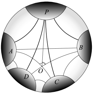
$\alpha$ $\beta$

Figure 3: A quintet of geodesics.

Using the trigonometry formulae for hyperbolic pentagons with four right-angles ([11], [4]), one obtains:

$$PA=-OP.OA.\cos(\alpha)+\widetilde{OP}.\widetilde{OA};\,\,\,\,\,\,\,\,PB=-OP.OB.\cos(\beta)+\widetilde{OP}.\widetilde{OB};$$

$$PC=-OP.OC.\cos(\pi-\alpha)+\widetilde{OP}.\widetilde{OC};\,\,\,\,\,\,\,\,PD=-OP.OD.\cos(\pi-\beta)+\widetilde{OP}.\widetilde{OD}.$$

These equations imply that:

$$PA.OC+PC.OA=\widetilde{OP}(\widetilde{OA}.OC+\widetilde{OC}.OA),$$

$$PB.OD+PD.OB=\widetilde{OP}(\widetilde{OD}.OB+\widetilde{OB}.OD).$$

And so

$$\frac{PA.OC+PC.OA}{PB.OD+PD.OB}=\frac{\widetilde{OA}.OC+\widetilde{OC}.OA}{\widetilde{OD}.OB+\widetilde{OB}.OD}=\frac{\widetilde{AC}}{\widetilde{BD}}.$$

∎

The following are special cases of the orthoquadrilateral relation.

Corollary 3.2.

(Ortho-isosceles trapezoid, orthorectangle, orthoparallelogram and orthokite relation of geodesics)

• If $AD=BC$ and $AC=BD$ then: $\dfrac{\overline{PA}^{2}-\overline{PB}^{2}}{\overline{AB}}=\dfrac{\overline{PD}^{2}-\overline{PC}^{2}}{\overline{CD}}.$

• If $AB=CD$, $AD=BC$ and $AC=BD$ then: $\overline{PA}^{2}+\overline{PC}^{2}=\overline{PB}^{2}+\overline{PD}^{2}.$

• If $AB=CD$, $AD=BC$ then: $\dfrac{PA+PC}{PB+PD}=\sqrt{\dfrac{AC-1}{BD-1}}.$

• If $AB=AD$, $CB=CD$ then: $PD+PB=\dfrac{2(AC.BC+AB)}{AC^{2}-1}.PA+\dfrac{2(AC.AB+BC)}{AC^{2}-1}.PC.$

Proof.

1. By using hyperbolic trigonometry for pentagons and right-angled hexagons, from the conditions $AD=BC$ and $AC=BD$, one can show that $OA=OB$, $OC=OD$ and then

$$\frac{PA.OC+PC.OA}{PB.OC+PD.OA}=1.$$

The last equality implies that:     $\dfrac{OA}{OC}=\dfrac{PA-PB}{PD-PC}=\dfrac{\overline{PA}^{2}-\overline{PB}^{2}}{\overline{PD}^{2}-\overline{PC}^{2}}.$

We also have

$$AB=-OA.OB.\cos(\alpha+\beta)+\widetilde{OA}.\widetilde{OB}=-OA^{2}.\cos(\alpha+\beta)+OA^{2}-1,$$

$$CD=-OC.OD.\cos(\alpha+\beta)+\widetilde{OC}.\widetilde{OD}=-OC^{2}.\cos(\alpha+\beta)+OC^{2}-1.$$

And so:      $\dfrac{\overline{AB}}{\overline{CD}}=\dfrac{OA}{OC}.$

3. By using hyperbolic trigonometry in pentagons and right-angled hexagons, from the conditions $AB=CD$ and $AD=BC$, one can show that $OA=OC=\overline{AC}$, $OC=OD=\overline{CD}$ and hence

$$\frac{PA+PC}{PB+PD}=\frac{\overline{BD}}{\overline{AC}}.\frac{\widetilde{AC}}{\widetilde{BD}}=\sqrt{\frac{\overline{AC}^{2}-1}{\overline{BD}^{2}-1}}.$$

4. Denote $b:=AB=AD$, $c:=CB=CD$ and $a:=AC$. One can show that $PD>PB$, then by applying the relation of quadruplet of geodesics (Corollary 3.1) for two quadruples $\{P;A,C,D\}$ and $\{P;A,C,B\}$, one has that $PB$ and $PD$ are two different roots of the following quadratic equation of variable $t$:

$$PA^{2}(c^{2}-1)+PC^{2}(b^{2}-1)+t^{2}(a^{2}-1)$$

$$=2(bc+a).PA.PC+2(ac+b).PA.t+2(ab+c).PC.t+a^{2}+b^{2}+c^{2}+2abc-1.$$

Thus one has the formula of the sum of two roots: $PD+PB=\dfrac{2(ac+b)}{a^{2}-1}.PA+\dfrac{2(ab+c)}{a^{2}-1}.PC.$ ∎

Remark. If $P$ is identical to one of the four geodesics, then the orthorectangle relation becomes the Pythagorean relation.

3.5 A quintet of horocycles

Let $A,P,B,C,D$ be five disjoint horocycles in $\mathbb{H}$ with a cyclic order. Each of them divides $\mathbb{H}$ into two domains such that the other four horocycles lie in the same domain. Let $O$ be the intersection between $AC$ and $BD$. Let $\alpha$ and $\beta$ be the angles between $OA,OP$ and $OB,OP$ respectively as in Figure 4.

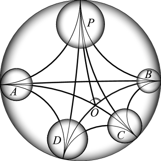
$\alpha$ $\beta$

Figure 4: A quintet of horocycles.

With the notations in Section 2, and using standard calculations in the upper half-plane model of hyperbolic plane, the following relations are obtained:

Lemma 3.6.

With $P,A,O$ and $\alpha$ defined above, one has

$$PA=OP.OA(1-\cos\alpha).$$

Applying Lemma 3.6 and the Penner's Ptolemy relation, one can compute $OA,OB,OC,OD$ in terms of $AC,BD,AD,AB,CD,CB$ as follows:

Lemma 3.7.

With $P,A,B,C,D$ and $O$ defined above, one obtains

$$OA=\frac{\overline{AC}}{2}\sqrt{\frac{\overline{AD}.\overline{AB}}{\overline{CD}.\overline{CB}}};\,\,\,OC=\frac{\overline{AC}}{2}\sqrt{\frac{\overline{CD}.\overline{CB}}{\overline{AD}.\overline{AB}}};\,\,\,OB=\frac{\overline{BD}}{2}\sqrt{\frac{\overline{BA}.\overline{BC}}{\overline{DA}.\overline{DC}}};\,\,\,OD=\frac{\overline{BD}}{2}\sqrt{\frac{\overline{DA}.\overline{DC}}{\overline{BA}.\overline{BC}}}.$$

Applying these above formulae and the argument as in the proof of Lemma 3.5, one obtains the following relation:

Lemma 3.8.

(Orthoquadrilateral relation of horocycles) With $P,A,B,C,D$ and $O$ defined above, one has

$$\frac{PA.OC+PC.OA}{PB.OD+PD.OB}=\frac{AC}{BD}.$$

Equivalently,

$$\frac{PA.\overline{CD}.\overline{CB}+PC.\overline{AD}.\overline{AB}}{PB.\overline{DA}.\overline{DC}+PD.\overline{BA}.\overline{BC}}=\frac{\overline{AC}}{\overline{BD}}.$$

Similarly, one also has the following properties of Penner's lambda lengths in special cases:

Corollary 3.3.

(Ortho-isosceles trapezoid, orthorectangle, orthoparallelogram relation of horocycles) With $P,A,B,C,D$ defined above, one has

• If $AD=BC$ and $AC=BD$ then: $\dfrac{\overline{PA}^{2}-\overline{PB}^{2}}{\overline{AB}}=\dfrac{\overline{PD}^{2}-\overline{PC}^{2}}{\overline{CD}}.$

• If $AB=CD$, $AD=BC$ and $AC=BD$ then: $\overline{PA}^{2}+\overline{PC}^{2}=\overline{PB}^{2}+\overline{PD}^{2}.$

• If $AB=CD$, $AD=BC$ then: $\dfrac{\overline{PA}^{2}+\overline{PC}^{2}}{\overline{PB}^{2}+\overline{PD}^{2}}=\dfrac{\overline{AC}}{\overline{BD}}.$

3.6 A unique formula in form of Cayley-Menger determinant

In this section one will see that all of the relations in previous sections can be put into a unique formula in form of Cayley-Menger determinant. Let $|UV|$ be the Euclidean distance between two arbitrary points $U$ and $V$ in a Euclidean space. In the field of distance geometry, the Cayley-Menger determinant allows us to compute the volume of an $n-$simplex in a Euclidean space in terms of the squares of all the distances between pairs of its vertices [13]. In a special case, if $A,B,C,D$ are four points in the Euclidean plane, one has a relation as follows:

$$\det\begin{bmatrix}0&1&1&1&1\\ 1&0&|AB|^{2}&|AC|^{2}&|AD|^{2}\\ 1&|AB|^{2}&0&|BC|^{2}&|BD|^{2}\\ 1&|AC|^{2}&|BC|^{2}&0&|CD|^{2}\\ 1&|AD|^{2}&|BD|^{2}&|CD|^{2}&0\end{bmatrix}=0.$$

If $A,B,C,D$ are four points in the hyperbolic plane, one has a similar formula [6] as follows:

$$\det\begin{bmatrix}-2&1&1&1&1\\ 1&0&\overline{AB}^{2}&\overline{AC}^{2}&\overline{AD}^{2}\\ 1&\overline{AB}^{2}&0&\overline{BC}^{2}&\overline{BD}^{2}\\ 1&\overline{AC}^{2}&\overline{BC}^{2}&0&\overline{CD}^{2}\\ 1&\overline{AD}^{2}&\overline{BD}^{2}&\overline{CD}^{2}&0\end{bmatrix}=0.$$

Now we consider geodesics and horocycles in the hyperbolic plane. Let $X$ be a curve of constant curvature in $\mathbb{H}$, denote by $\kappa_{X}$ the geodesic curvature of $X$. Thus $\kappa_{X}=0$ or $1$ if $X$ is a geodesic or a horocycle respectively. The relations of quadruplet of geodesics/horocycles in Lemma 3.4 can be written in a unique form as follows

Theorem 3.4.

Let $A,B,C,D$ be four disjoint geodesics/horocycles, each of them divides $\mathbb{H}$ into two domains such that the other three lie in the same domain. Then

$$\det\begin{bmatrix}2&1-\kappa_{A}&1-\kappa_{B}&1-\kappa_{C}&1-\kappa_{D}\\ 1-\kappa_{A}&0&\overline{AB}^{2}&\overline{AC}^{2}&\overline{AD}^{2}\\ 1-\kappa_{B}&\overline{AB}^{2}&0&\overline{BC}^{2}&\overline{BD}^{2}\\ 1-\kappa_{C}&\overline{AC}^{2}&\overline{BC}^{2}&0&\overline{CD}^{2}\\ 1-\kappa_{D}&\overline{AD}^{2}&\overline{BD}^{2}&\overline{CD}^{2}&0\end{bmatrix}=0.$$

Remark. We suspect that the result can be generalized to higher dimensions in the following form: Let $U$ and $V$ be two arbitrarily disjoint hyperbolic spaces or horoballs of co-dimension 1 in $\mathbb{H}^{n}$. Denote by $\kappa_{U}$ and $\kappa_{V}$ the geodesic curvatures of $U$ and $V$ respectively. We define a weight function between $U$ and $V$ which is a generalized version of the half-trace and the half of Penner's lambda length of the distance between $U$ and $V$ as follows.

$$\overline{UV}:=\frac{e^{\frac{1}{2}d_{\mathbb{H}^{n}}(U,V)}+(1-\kappa_{U})(1-\kappa_{V})e^{-\frac{1}{2}d_{\mathbb{H}^{n}}(U,V)}}{2}$$

Let $\{A_{1},A_{2},...,A_{k},A_{k+1},A_{k+2}\}$ be the set of $k+2$ disjoint hypersurfaces of constant geodesic curvatures in $n$-dimensional hyperbolic space $\mathbb{H}^{n}$ ($k\geq n$), each of them divides $\mathbb{H}^{n}$ into two domains such that the other $k+1$ hypersurfaces lie in the same domain. If $\kappa_{A_{i}}\in\{0,1\}$ for all $i\in\{1,2,...,k+2\}$, then

$$\det\begin{bmatrix}2&1-\kappa_{A_{1}}&1-\kappa_{A_{2}}&1-\kappa_{A_{3}}&\cdots&1-\kappa_{A_{k+2}}\\ 1-\kappa_{A_{1}}&0&\overline{A_{1}A_{2}}^{2}&\overline{A_{1}A_{3}}^{2}&\cdots&\overline{A_{1}A_{k+2}}^{2}\\ 1-\kappa_{A_{2}}&\overline{A_{2}A_{1}}^{2}&0&\overline{A_{2}A_{3}}^{2}&\cdots&\overline{A_{2}A_{k+2}}^{2}\\ 1-\kappa_{A_{3}}&\overline{A_{3}A_{1}}^{2}&\overline{A_{3}A_{2}}^{2}&0&\cdots&\overline{A_{3}A_{k+2}}^{2}\\ \vdots&\vdots&\vdots&\vdots&\ddots&\vdots\\ 1-\kappa_{A_{k+2}}&\overline{A_{k+2}A_{1}}^{2}&\overline{A_{k+2}A_{2}}^{2}&\overline{A_{k+2}A_{3}}^{2}&\cdots&0\end{bmatrix}=0.$$

4 Orthotree, identity relations and r-orthoshapes

For simplicity, in this section we only present a tree structure and identity relations of orthogeodesics on a hyperbolic surface with its boundary consisting of simple closed geodesics.

4.1 Orthotree

In [19], Labourie and Tan generalized Bowditch's method to give a planar tree coding of oriented simple orthogeodesics on a hyperbolic surface by doing special flips on an orthotriangulation of the surface. In this section, we extend their method to obtain a construction which can be applied for any suitable subset of the set of oriented orthogeodesics starting from a boundary component. This construction may be useful for studying coherent markings introduced by Parlier in [23].

Let $S$ be an orientable hyperbolic surface with boundary $\partial S$ consisting of simple closed geodesics. Let $\eta_{\frac{0}{1}}$ and $\eta_{\frac{1}{1}}$ be two oriented orthogeodesics starting from a simple closed geodesic $\alpha$ at the boundary of $S$. The starting points of these two orthogeodesics divides $\alpha$ into two open subsegments, namely $\alpha_{1}$ and $\alpha_{2}$. Suppose that $\alpha_{1}\neq\varnothing$. Denote by $\mathcal{O}_{\alpha_{1}}$ the set of oriented orthogeodesics starting from $\alpha_{1}$. The orientation of $S$ gives an order on $\mathcal{O}_{\alpha_{1}}$ independent of the hyperbolic structure. In particular, the order on $\mathcal{O}_{\alpha_{1}}$ is defined by the order of the starting points of $\mathcal{O}_{\alpha_{1}}$ on $\alpha_{1}$. By that, if $\eta_{x}$, $\eta_{y}$ and $\eta_{z}$ are three elements in $\mathcal{O}_{\alpha_{1}}$ and the starting point of $\eta_{y}$ lies between $\eta_{x}$ and $\eta_{z}$ with respect to the subsegment $\alpha_{1}$, we say $\eta_{y}$ lies between $\eta_{x}$ and $\eta_{z}$.

Labelling elements in a subset of $\mathcal{O}_{\alpha_{1}}$:

A Farey pair $(\frac{p}{q},\frac{m}{n})$ is a pair of two reduced fractions $\frac{p}{q}$ and $\frac{m}{n}$ such that $\frac{0}{1}\leq\frac{p}{q}<\frac{m}{n}\leq\frac{1}{1}$ and $qm-pn=1$. Their Farey sum is defined as $\frac{p}{q}\oplus\frac{m}{n}:=\frac{p+m}{q+n}$. Thus $\frac{p}{q}<\frac{p}{q}\oplus\frac{m}{n}<\frac{m}{n}$. Furthermore, $(\frac{p}{q},\frac{p}{q}\oplus\frac{m}{n})$ and $(\frac{p}{q}\oplus\frac{m}{n},\frac{m}{n})$ become two other Farey pairs.

Let $G$ be a countable subset of $\mathcal{O}_{\alpha_{1}}$ such that for any two arbitrary elements of $G$, there are infinitely many other elements of $G$ lying between them. For example, $G$ can be taken as the set $\mathcal{O}_{\alpha_{1}}$ itself or the set of simple oriented orthogeodesics starting from $\alpha_{1}$ when $\eta_{\frac{0}{1}}$, $\eta_{\frac{1}{1}}$ and $\alpha_{1}$ are chosen suitably. We label elements in the set $G$ by rational numbers between $0$ and $1$ as follows:

Step 1: Take an arbitrary element in $G$ and name it by $\eta_{\frac{0}{1}\oplus\frac{1}{1}}$ or equivalently $\eta_{\frac{1}{2}}$. The starting point of this element divides $\alpha_{1}$ into two disjoint open subsegments. By abuse of notation, we denote these two subsegments by $(\eta_{\frac{0}{1}},\eta_{\frac{1}{2}})$ and $(\eta_{\frac{1}{2}},\eta_{\frac{1}{1}})$.

Step $k\geq 2$: $\alpha_{1}$ is divided into $2^{k-1}$ disjoint open subsegments of the form $(\eta_{\frac{p_{1}}{q_{1}}},\eta_{\frac{p_{2}}{q_{2}}})$ where $(\frac{p_{1}}{q_{1}},\frac{p_{2}}{q_{2}})$ is a Farey pair. Denote by $G(\eta_{\frac{p_{1}}{q_{1}}},\eta_{\frac{p_{2}}{q_{2}}})$ the set of oriented orthogeodesics in $G$ starting from the subsegment $(\eta_{\frac{p_{1}}{q_{1}}},\eta_{\frac{p_{2}}{q_{2}}})$. Similarly to step 1, we take an arbitrary element in $G(\eta_{\frac{p_{1}}{q_{1}}},\eta_{\frac{p_{2}}{q_{2}}})$ and name it by $\eta_{\frac{p_{1}}{q_{1}}\oplus\frac{p_{2}}{q_{2}}}$ or equivalently $\eta_{\frac{p_{1}+p_{2}}{q_{1}+q_{2}}}$. We do it for all other subsegments and obtain $2^{k}$ new disjoint open subsegments.

The above labelling gives an order-preserving injection

$$\mathring{\Psi}_{1}:\mathbb{Q}\cap(0,1)\to G.$$

This map can be extended naturally to a map

$$\Psi_{1}:\mathbb{Q}\cap[0,1]\to G\cup\{\eta_{\frac{0}{1}},\eta_{\frac{1}{1}}\}.$$

Note that if $\eta_{\frac{0}{1}}$ and $\eta_{\frac{1}{1}}$ are distinct oriented orthogeodesics, then $\Psi_{1}$ is also an order-preserving injection.

The bijectivity:

For each orthogeodesic $X$, we denote $h(X):=\frac{1}{2}\log\left(\frac{X+1}{X-1}\right)$ the radius of the stable neighborhood of $X$. In each step $k\geq 1$, we have $2^{k-1}$ disjoint open subsegments of $\alpha_{1}$. Let $(X,Y)$ be one of these subsegments and let $\ell(X,Y)$ be the length of this subsegment. Let $m(X,Y):=\ell(X,Y)-h(X)-h(Y)$ the modified length of the segment $(X,Y)$. We denote by $m_{k}$ the maximum of the modified lengths of the associated $2^{k-1}$ disjoint subsegments in step $k$, then

Lemma 4.1.

The map $\mathring{\Psi}_{1}$ is an order-preserving bijection if $m_{k}\to 0$ as $k\to\infty$.

Proof.

Assume that $X$ is an oriented orthogeodesic in $G$ such that $\mathring{\Psi}_{1}(p/q)\neq X$ for all $p/q\in\mathbb{Q}\cap(0,1)$. Let $(Y_{k},Z_{k})$ be the subsegment containing $X$ at step $k$. It is easy to see that $m(Y_{k},Z_{k})\geq 2h(X)$ for all $k\geq 1$, a contradiction to the fact that $m_{k}\to 0$ as $k\to\infty$. ∎

In the example below, we will present another way to define $\mathring{\Psi}_{1}$ based on a given orthotriangulation of $S$ which is closely related to the construction in [19].

Labelling complementary regions of a tree:

Let $T_{1}$ be a planar rooted trivalent tree whose the first vertex is of valence 1, and all other vertices are of valence 3. We visualize it by embedding $T_{1}$ to the lower half-plane with the root is located at the origin (see Figure 6 for an example). Let $E(T_{1})$ be the set of edges of $T_{1}$. Each edge of the tree has two sides associated to two distinct complementary regions of the tree. Let $\Omega(T_{1})$ be the set of complementary regions of the tree. We label elements in $\Omega(T_{1})$ as follows: The two initial regions is labeled by fraction numbers $\frac{0}{1}$ and $\frac{1}{1}$. Since each vertex except the root has three regions surrounding it, so if we know the labels of two of them, we can label the third region by their Farey sum. Thus, one obtains a bijection

$$\Psi_{2}:\mathbb{Q}\cap[0,1]\to\Omega(T_{1}).$$

By this map, the order on $\mathbb{Q}\cap[0,1]$ then descents to an order on $\Omega(T_{1})$. Denote by $\mathring{\Omega}(T_{1})$ the set $\Psi_{2}(\mathbb{Q}\cap(0,1))$. Combining with Lemma 4.1, we obtain the following theorem:

Theorem 4.1.

If $m_{k}\to 0$ as $k\to\infty$, the map $\mathring{\Psi}:=\mathring{\Psi}_{1}\circ\Psi_{2}^{-1}|_{\mathring{\Omega}(T_{1})}$ is an order-preserving bijection from $\mathring{\Omega}(T_{1})$ to $G$. Furthermore if $\eta_{\frac{0}{1}}$ and $\eta_{\frac{1}{1}}$ are distinct, then the map $\Psi:=\Psi_{1}\circ\Psi_{2}^{-1}$ is also an order-preserving bijection.

Therefore, the map $\Psi$ gives us a label of $\Omega(T_{1})$ by the set $G\sqcup\{\eta_{\frac{0}{1}}\}\sqcup\{\eta_{\frac{1}{1}}\}$.

Labelling edges of the tree $T_{1}$:

Let $Y$ and $Z$ be two arbitrary complementary regions of $T_{1}$. Thus, $\Psi(Y)$ and $\Psi(Z)$ are two oriented orthogeodesics starting from $\alpha_{1}$ and define a open subsegment, namely $(\Psi(Y),\Psi(Z))$, of $\alpha_{1}$. The two orthogeodesics $\Psi(Y)$ and $\Psi(Z)$ then together with the subsegment $(\Psi(Y),\Psi(Z))$ define a unique orthogeodesic denoted by $F(\Psi(Y),\Psi(Z),\alpha_{1})$ such that they are four sides of an orthotriangle on $S$. Note that $F(\Psi(Y),\Psi(Z),\alpha_{1})$ and $(\Psi(Y),\Psi(Z))$ are two opposite sides in this orthotriangle. If $x$ is an edge of the tree $T_{1}$ with two neighboring complementary regions $Y$ and $Z$, then we label $x$ by the orthogeodesic $F(\Psi(Y),\Psi(Z),\alpha_{1})$.

A simple example:

Let $\Delta$ be an orthotriangulation on $S$. Suppose that $\eta_{\frac{0}{1}}$, $\eta_{\frac{1}{1}}$ and $\alpha_{1}$ defined as above are three sides of an orthotriangle in $\Delta$. For simplicity, we will take $G$ as the set $\mathcal{O}_{\alpha_{1}}$ itself. For any element $X\in\mathcal{O}_{\alpha_{1}}$, we denote by $N(X)$ the number of intersections of $X$ with the orthobasis of $\Delta$. We define the associated map $\Psi_{1}$ as follows:

Step 1: Take an element $X$ in $\mathcal{O}_{\alpha_{1}}$ such that $N(X)$ is minimal. We name it by $\eta_{\frac{0}{1}\oplus\frac{1}{1}}$ or equivalently $\eta_{\frac{1}{2}}$. The starting point of this element divides $\alpha_{1}$ into two disjoint open subsegments, denoted by $(\eta_{\frac{0}{1}},\eta_{\frac{1}{2}})$ and $(\eta_{\frac{1}{2}},\eta_{\frac{1}{1}})$.

Step $k\geq 2$: $\alpha_{1}$ is divided into $2^{k-1}$ disjoint open subsegments of the form $(\eta_{\frac{p_{1}}{q_{1}}},\eta_{\frac{p_{2}}{q_{2}}})$ where $(\frac{p_{1}}{q_{1}},\frac{p_{2}}{q_{2}})$ is a Farey pair. Denote by $G(\eta_{\frac{p_{1}}{q_{1}}},\eta_{\frac{p_{2}}{q_{2}}})$ the set of oriented orthogeodesics in $G$ starting from the subsegment $(\eta_{\frac{p_{1}}{q_{1}}},\eta_{\frac{p_{2}}{q_{2}}})$. Apply step 1 for each of these subsegments, one obtains $2^{k}$ new disjoint subsegments.

By this construction, we exhaust all elements in $\mathcal{O}_{\alpha_{1}}$. Thus, $\Psi_{1}$ is an order-preserving bijection from $\mathbb{Q}\cap[0,1]$ to $\mathcal{O}_{\alpha_{1}}\cup\{\eta_{\frac{0}{1}},\eta_{\frac{1}{1}}\}.$ Hence $\Psi:=\Psi_{1}\circ\Psi_{2}^{-1}$ gives us a label of $\Omega(T_{1})$ by the set $\mathcal{O}_{\alpha_{1}}\cup\{\eta_{\frac{0}{1}},\eta_{\frac{1}{1}}\}.$ By looking at the universal cover, one can also see that if $X$ is a chosen element in step $k$, then $N(X)=k$.

Furthermore, if $\Delta$ be a standard orthotriangulation (see Definition 1.3), each oriented orthogeodesic in $\mathcal{O}_{\alpha_{1}}$ can also be encoded by its crossing sequence with the orthobasis of $\Delta$. Note that two oriented orthogeodesics in $\mathcal{O}_{\alpha_{1}}$ are of the same crossing sequence (word) iff they are two different directions of an orthogeodesic with a symmetric word. This labeling is useful when we only care of the ortholength spectrum. Due to the labeling of edges, each path of edges starting from the root is associated to a continuous sequence of elements in the orthobasis (crossing sequence). We label the associated complementary region of the path by capitalizing the word formed from the crossing sequence (see Figure 6 for a tree with labels on edges and complementary regions and see Figure 7 for an example of the crossing sequence of an orthogeodesic).

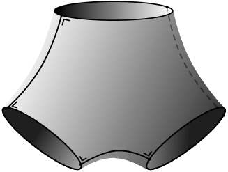
$\alpha_{1}$ $\alpha_{2}$ $\beta_{1}$ $\beta_{2}$ $\gamma_{1}$ $\gamma_{2}$ $b$ $a$ $c$

Figure 5: A standard orthotriangulation on a pair of pants.

Figure 6: Labeling the tree of oriented orthogeodesics starting at $\alpha_{1}$.

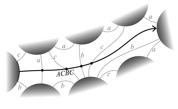
$\alpha_{1}$

Figure 7: A lift of an oriented orthogeodesic $(ACBC)$ starting at $\alpha_{1}$.

Note that we have only defined the tree of oriented orthogeodesics starting at a subsegment of a simple closed geodesic $\alpha$ at the boundary of a surface. Since the orthobasis of $\Delta$ divides $\alpha$ into a finite number of disjoint open subsegments. One can glue the roots of suitable labeled trees associated to all the subsegments in a cyclic order to get a planar rooted trivalent tree of all oriented orthogeodesics starting from $\alpha$.

4.2 Identity relations

4.2.1 Recursive formula and vertex relation

Let $X,Y,Z$ be three complementary regions surrounding a vertex $v$ (not at the root) of the tree $T_{1}$. Let $x,y,z$ be three edges which intersect $X,Y,Z$ respectively at only $v$. Suppose that the set of edges of $T_{1}$ is oriented outwards from the root. If the end point of the oriented edge $x$ and the starting point of the oriented edges $y$ and $z$ coincide at $v$ (see Figure 8), by the Ptolemy relation of geodesics in Lemma 3.2, one can compute $X$ in term of $Y,Z,x,y,z$:

$$X=\frac{(xy+z)Y+(xz+y)Z+\sqrt{(x^{2}+y^{2}+z^{2}+2xyz-1)(x^{2}+Y^{2}+Z^{2}+2xYZ-1)}}{x^{2}-1}.$$

$x$ $y$ $z$ $v$ $X$ $Y$ $Z$

Figure 8: Positions of $X,Y,Z,x,y,z$.

Note that by Corollary 3.1, we also have a vertex relation as follows:

$$(x^{2}-1)X^{2}+(y^{2}-1)Y^{2}+(z^{2}-1)Z^{2}-2(xy+z)XY-2(yz+x)YZ-2(xz+y)XZ$$

$$=x^{2}+y^{2}+z^{2}+2xyz-1.$$

4.2.2 Isosceles trapezoid, rectangle, kite, parallelogram and edge relations

We define the weight function $UV:=\text{weight}(U,V)$ between two complementary regions $U$ and $V$ to be the hyperbolic cosine of the length of the orthogeodesic $F(\Psi(U),\Psi(V),\alpha_{1})$ as defined in Section 4.1. Let $X,Y,Z,T$ be four complementary regions, by Corollary 3.2 in Section 3, we have the following relations:

• If $XT=YZ$, and $XZ=YT$, then: $\dfrac{X-Y}{\sqrt{XY+1}}=\dfrac{Z-T}{\sqrt{ZT+1}}.$

• If $XT=YZ$, $XY=ZT$, and $XZ=YT$, then: $X+T=Y+Z.$

• If $XY=XT$, and $ZY=ZT$, then: $T+Y=\dfrac{2(XZ.YZ+XY)}{(XZ)^{2}-1}X+\dfrac{2(XZ.XY+YZ)}{(XZ)^{2}-1}Z.$

• If $XY=ZT$, and $XT=YZ$, then: $X+Z=(Y+T)\sqrt{\dfrac{XZ-1}{YT-1}}.$

Furthermore, one obtains edge relations of orthogeodesics on certain special surfaces as in the following examples.

Example 1: Edge relations on a pair of pants. Denote $\{a,b,c\}$ the standard orthobasis of a pair of pants that is the set of shortest simple orthogeodesics connecting two distinct boundary components. This orthobasis cuts each boundary geodesic component into two geodesic segments of equal length. The six resulting segments are denoted by $\alpha_{1},\alpha_{2},\beta_{1},\beta_{2},\gamma_{1},\gamma_{2}$ as in Figure 5. Let $T_{1}$ be the tree of oriented orthogeodesics starting from $\alpha_{1}$. As in Figure 5, $b$ and $c$ are on the left and the right of the segment $\alpha_{1}$ and $a$ is opposite to $\alpha_{1}$. Each edge of $T_{1}$ is labeled by either $a$ or $b$ or $c$ following the grammar of the dual graph of the orthotriangulation. We also use words formed from the capital letters $A,B,C$ to label the complemetary regions of $T_{1}$ except for the two initial regions. Figure 6 is an illustration of the tree $T_{1}$.

Edge relations are special cases of orthokite relations when four edges of the orthokite are elements in the standard orthobasis of a pair of pants. There are four regions surrounding each edge - except for the edge with an end point at the root. We choose arbitrarily an edge $x\in\{a,b,c\}$ with four surrounding regions $X_{1},Y,Z,X_{2}$ with $Y\cap Z=x$. Due to the standard orthobasis of a pair of pants, $X_{1}Y=X_{2}Y=:z$ and $X_{1}Z=X_{2}Z=:y$, where $y,z$ are distinct elements in $\{a,b,c\}-\{x\}$. Thus one can denote the labels of $X_{1}\cap Y$, $X_{1}\cap Z$, $X_{2}\cap Y$, $X_{2}\cap Z$ to be $z,y,z,y$ respectively (see e.g. Figure 9). We have an edge relation of orthogeodesics on a pair of pants:

$$X_{1}+X_{2}=\frac{2(xy+z)}{x^{2}-1}Y+\frac{2(xz+y)}{x^{2}-1}Z.$$ (3)

$Y$ $x$ $y$ $z$ $y$ $z$ $X_{1}$ $Z$ $X_{2}$

Figure 9: Positions of $X_{1},X_{2},Y,Z,x,y,z$ in the case of a pair of pants.

Example 2: Edge relations on a one-holed torus. We denote $\{a,b,c\}$ to be an arbitrary orthobasis of a one-holed torus that is the set of three non-crossing simple orthogeodesics. This orthobasis cuts the boundary geodesic component of the one-holed torus into six geodesic segments.

$Y$ $x$ $y$ $z$ $z$ $y$ $X_{1}$ $Z$ $X_{2}$

Figure 10: Positions of $X_{1},X_{2},Y,Z,x,y,z$ in the case of a one-holed torus.

Let $T_{1}$ be the tree of oriented orthogeodesics starting from one of these six segments. There are four regions surrounding each edge - except for the edge with an end point at the root. We choose arbitrarily an edge $x\in\{a,b,c\}$ with four surrounding regions $X_{1},Y,Z,X_{2}$ with $Y\cap Z=x$. We have $X_{1}Y=X_{2}Z=:y$ and $X_{1}Z=X_{2}Y=:z$, where $y,z$ are distinct elements in $\{a,b,c\}-\{x\}$. Thus one can denote the labels of $X_{1}\cap Y$, $X_{1}\cap Z$, $X_{2}\cap Y$, $X_{2}\cap Z$ to be $y,z,z,y$ respectively (see Figure 10). Then by the parallelogram relation, one has

$$X_{1}+X_{2}=(Y+Z)\sqrt{\frac{X_{1}X_{2}-1}{YZ-1}}.$$

Note that $X_{1}X_{2}$ is the cosh of the length of the simple orthogeodesic with label $X$ crossing the edge $x$. Thus one can use the recursive formula (Section 4.2.1) to compute $X_{1}X_{2}$ in terms of $x,y,z$ as follows:

$$X_{1}X_{2}=\frac{(xy+z)y+(xz+y)z+x^{2}+y^{2}+z^{2}+2xyz-1}{x^{2}-1}=\frac{(y+z)^{2}}{x-1}+1.$$

Note that $YZ=x$, thus we have an edge relation of orthogeodesics on a one-holed torus:

$$X_{1}+X_{2}=\frac{y+z}{x-1}(Y+Z).$$ (4)

In the next section, we will use reflection involutions on immersed pairs of pants to construct a family of ortho-isosceles-trapezoids, orthorectangles and orthokites on a general hyperbolic surface.

4.3 A construction of r-orthoshapes using reflection involutions

Let $P$ be a pair of pants with boundary components $o_{1},o_{2},o_{3}$. Let $a,b,c,A,B,C$ be simple orthogeodesics connecting two elements in each of pairs $(o_{2},o_{3})$, $(o_{1},o_{3})$, $(o_{1},o_{2})$, $(o_{1},o_{1})$, $(o_{2},o_{2})$, $(o_{3},o_{3})$ respectively. Note that $a,b,c$ are also called the seams of $P$. Let $r$ be the unique orientation-reversing isometry over $P$ which fixes $a,b,c$ pointwisely. Note that if $\ell(o_{1})$, $\ell(o_{2})$ and $\ell(o_{3})$ are pairwise different, then the isometry group of $P$ is $\{id,r\}$ with $r^{2}=id$. Let $\{i,j,k\}=\{1,2,3\}$. If $\ell(o_{i})=\ell(o_{j})$, let $r_{k}$ be the unique orientation-reserving isometry over $P$ which fixes $o_{k}$ and interchanges $o_{i}$ with $o_{j}$. The set of fixed points of each of isometries $r_{1},r_{2},r_{3}$ forms each of orthogeodesics $A,B,C$ respectively. Note that if $\ell(o_{i})=\ell(o_{j})\neq\ell(o_{k})$, the isometry group of $P$ will be $\{id,r_{k},r,r\circ r_{k}\}$ with $r^{2}=r_{k}^{2}=(r\circ r_{k})^{2}=id$ and $r\circ r_{k}=r_{k}\circ r$. A thorough treatment on pairs of pants can be found in chapter 3 of Buser's book [11]. Before going to the construction of r-orthoshapes, we need the following notions:

• $P$ is called an isosceles pair of pants if it has two boundary components of the same length. It is called a regular pair of pants if its three boundary components are of the same length.

• A reflection involution $i$ on $P$ is an orientation-reversing isometry on $P$ which fixes a simple orthogeodesic pointwisely (the ``symmetry axis'' of $i$). For example: $r$ is a reflection involution on $P$ and it has three symmetry axes $a,b,c$. If $\ell(o_{i})=\ell(o_{j})$, then $r_{k}$ is another reflection involution on $P$.

Let $\Sigma$ be an oriented topological surface with punctures and negative Euler characteristic. A point in $\mathcal{T}(\Sigma)$ can be represented by a hyperbolic surface, namely $S$, with $\partial{S}$ consisting of simple closed geodesics and/or cusps such that the interior of $S$ is homeomorphic to $\Sigma$. In the following, we construct a class of r-orthoshapes on $\Sigma$ coming from reflection involutions on immersed pairs of pants.

Lemma 4.2.

An orthogeodesic $\gamma$ and its reflection through a reflection involution form infinitely many r-ortho-isosceles-trapezoids and r-orthokites on $\Sigma$.

Proof.

Without loss of generality, one can assume that $\gamma$ is a common orthogeodesic of $S\in\mathcal{T}(\Sigma)$ and $P$ where $P$ is an immersed pair of pants on $S$. Let $r$ be a reflection involution on $P$ which fixes its seams. Lifting to the universal cover of $S$. The lift of $P$ has an injective simple connected fundamental domain. Let $\tilde{a}$ be a lift of a symmetry axis of $r$ (i.e. a lift of the seam $a$ of $P$). A lift of $\gamma$ and its reflection through $\tilde{a}$ form either an r-orthokite or an r-ortho-isosceles-trapezoid on the universal cover of $S$ depending on the chosen lift of $\gamma$. Since there are infinitely many lifts of $\gamma$, there are also infinitely many r-ortho-isosceles-trapezoids and r-orthokites on the universal cover of $S$ such that their projection to the surface gives infinitely many different r-ortho-isosceles-trapezoids and r-ortho kites. ∎

The special case of an r-ortho-isosceles-trapezoid is an r-orthorectangle happened in an immersed isosceles pair of pants when there is a reflection involution between the other pair of the opposite orthogeodesics in the r-ortho-isosceles-trapezoid.

Lemma 4.3.

The endpoints of orthogeodesics forming an r-orthorectangle are always on the same boundary component of $\Sigma$.

Proof.

Let $ABCD$ be an r-orthorectangle in which each pair of orthogeodesics $(AB,CD)$, $(BC,DA)$, $(AC,BD)$ are length equivalent. If the endpoints of $AB$, $CD$, $BC$, $DA$ are on two distinct boundary components, say $\beta_{1}$ and $\beta_{2}$, of $\Sigma$. Then both endpoints of $AC$ are on the same boundary component, say $\beta_{1}$ (without loss of generality). Thus both endpoints of $BD$ have to be on $\beta_{2}$. It contradicts the fact that $(AC,BD)$ are length equivalent. ∎

Lemma 4.4.

There are infinitely many r-orthorectangles on $\Sigma$.

Proof.

Let $\gamma$ be an orthogeodesic with its endpoints on the same boundary component of $S\in\mathcal{T}(\Sigma)$. Let $P$ be an immersed isosceles pair of pants on $S$ with $\gamma$ as one of its seams and two geodesic boundary components of $P$, say $o_{1}$ and $o_{2}$, are embedded to a single boundary component of $S$. Let $r$ and $r_{3}$ be two reflection involutions on $P$ where $r$ fixes the seams of $P$ and $r_{3}$ interchanges $o_{1}$ and $o_{2}$. Let $\eta$ be the symmetry axis of $r_{3}$, hence $\eta$ is an arc with its endpoints on the third boundary of $P$ and it is perpendicular to $\gamma$ at their midpoints. Let $\alpha$ be an orthogeodesic in $P$ with its ends on $o_{1}$ such that $\alpha$ wraps $n$ times around $o_{2}$ and zero time around $o_{1}$, where $n\geq 2$. Then $\beta:=r_{3}(\alpha)$ is an orthogeodesic in $P$ with its ends on $o_{2}$ and it wraps $n$ times around $o_{1}$ without wraping around $o_{2}$. Lifting to the universal cover of $S$. The lift of $P$ has an injective simple connected fundamental domain. Under these conditions, one is always able to find lifts of $\gamma$, $\eta$, $\alpha$ and $\beta$, namely $\tilde{\gamma}$, $\tilde{\eta}$, $\tilde{\alpha}$ and $\tilde{\beta}$, such that

• $\tilde{\eta}$, $\tilde{\alpha}$ and $\tilde{\beta}$ are disjoint,

• $\tilde{\beta}$ is the reflection of $\tilde{\alpha}$ through $\tilde{\eta}$ on the universal cover of $S$,

• $\tilde{\gamma}$ is perpendicular to $\tilde{\eta}$ at their midpoints, and perpendicular to $\tilde{\alpha}$ and $\tilde{\beta}$ at the midpoints of $\tilde{\alpha}$ and $\tilde{\beta}$.

Thus $\tilde{\alpha}$, $\tilde{\beta}$ together with two other associated orthogeodesics form an r-ortho rectangle on the universal cover of $S$. Projecting it back to $S$ one obtains an r-ortho rectangle on $S$. Since $n$ can be chosen arbitrarily in $\mathbb{N}_{\geq 2}$ and even more than that $\gamma$ can be chosen arbitrarily in the set of orthogeodesics with endpoints on the same boundary component of $S$, there are infinitely many r-orthorectangles on $S$. ∎

Lemma 4.5.

There is no r-orthosquare on $\Sigma$.

Proof.

Suppose that there exists $\mathbb{O}:=XYZT$ an r-orthosquare on $\Sigma$. We consider a hyperbolic structure $S^{*}$ on $\Sigma$ which satisfies:

• $S^{*}$ is a cusped surface.

• There is a truncated orthobasis (i.e. a decorated ideal triangulation) on $S^{*}$ including only orthogeodesics of lambda length 1.

Note that if we lift this decorated ideal triangulation of $S^{*}$ to $\mathbb{H}$, we obtains the Farey tessellation with Ford circles. Also note that by Penner's Ptolemy relation (see Equation 1), the tree of lambda lengths of orthogeodesics on $S^{*}$ is the tree of Fibonacci function (see [8] for a definition). Thus the lambda length of any orthogeodesics on $S^{*}$ is always an integer (also see [27] for a direct computation on the Farey decoration).

Again by Penner's Ptolemy relation, $\lambda(X,Z)\lambda(Y,T)=\lambda(X,Y)\lambda(Z,T)+\lambda(X,T)\lambda(Y,Z)$. Thus $\lambda(X,Z)=\lambda(X,Y)\sqrt{2}$ since $\mathbb{O}$ is an orthosquare on $S^{*}$. It contradicts the fact that the lambda length of any orthogeodesic on $S^{*}$ is always an integer. ∎

5 Applications

In this section we present some applications from the study of the tree structure on the set of orthogeodesics.

5.1 A combinatorial proof of Basmajian's identity

Let $S$ be a hyperbolic surface of totally geodesic boundary, Basmajian's identity on $S$ is as follows:

$$\ell(\partial{S})=\sum_{\eta}2\log(\coth(\ell(\eta)/2)),$$

where the sum runs over the set of orthogeodesics on the surface. This identity was proved by using elementary hyperbolic geometry and the fact that the limit set of a non-elementary second kind Fuchsian group is of 1- dimensional measure zero. In this section, we will present a combinatorial proof of Basmajian's identity in the case of a hyperbolic surface with totally geodesic boundary.

Let $T_{1}$ be a rooted trivalent tree whose first vertex is of valence 1, and all other vertices are of valence 3. We visualize it by embedding $T_{1}$ in the lower half-plane with the root is located at the origin (see Figure 6). Let $E(T_{1})$ be the set of edges of $T_{1}$ where each edge is oriented outwards from the root. Let $\Omega(T_{1})$ be the set of complementary regions of $T_{1}$. Similarly to the definition of the Markoff map in [7], one can define a map $\Phi:E(T_{1})\sqcup\Omega(T_{1})\to(1,\infty)$ which has a harmonic relation at any vertex except at the root of the tree as follows:

$$\operatorname{arccosh}\frac{x+YZ}{\sqrt{(Y^{2}-1)(Z^{2}-1)}}=\operatorname{arccosh}\frac{z+XY}{\sqrt{(X^{2}-1)(Y^{2}-1)}}+\operatorname{arccosh}\frac{y+XZ}{\sqrt{(X^{2}-1)(Z^{2}-1)}},$$

where $x,y,z,X,Y,Z$ are the abbreviations of $\Phi(x),\Phi(y),\Phi(z),\Phi(X),\Phi(Y),\Phi(Z)$ respectively and they are as in Figure 8. Note that the idea of this harmonic relation comes from Lemma 3.1. We define a function $h$ on $\Omega(T_{1})$ as follows:

$$h(X):=\operatorname{arccosh}\left(\frac{X}{\sqrt{X^{2}-1}}\right)=\frac{1}{2}\log\left(\frac{X+1}{X-1}\right).$$

A triple $(x,Y,Z)\in E(T_{1})\times\Omega(T_{1})\times\Omega(T_{1})$ is called an edge region triple if $x=Y\cap Z$ (i.e. $Y,Z\in\Omega(T_{1})$ are two neighboring complementary regions of $x\in E(T_{1})$). We define a function $f$ on the set of edge region triples as follows:

$$f(x,Y,Z):=\operatorname{arccosh}\left(\frac{x+YZ}{\sqrt{(Y^{2}-1)(Z^{2}-1)}}\right).$$

Note that $\lim_{Y\to\infty}f(y,X,Y)=\lim_{Z\to\infty}f(z,X,Z)=h(X).$ The harmonic relation can be rewritten as:

$$f(x,Y,Z)=f(y,X,Z)+f(z,X,Y),$$

for all $X,Y,Z,x,y,z$ as in Figure 8. Thus we have a Green formula:

$$\sum_{x\in C_{n}}f(x,Y,Z)=f(x_{0},Y_{0},Z_{0}),$$

where $(x_{0},Y_{0},Z_{0})$ is the initial edge region triple (i.e., $x_{0}\in E(T_{1})$ is the initial edge from the root, $Y_{0},Z_{0}\in\Omega(T_{1})$ are two neighboring complementary regions of $x_{0}$), and $C_{n}$ is the set of edges at combinatorial distance $n\in\mathbb{N}$ from the root. We use Bowditch's argument to prove Basmajian's identity:

Theorem 5.1.

(Basmajian's identity for $T_{1}$) If $\sup\{\Phi(x)|x\in E(T_{1})\}<\infty$, then

$$\sum_{X\in\Omega(T_{1})}2h(X)=h(Y_{0})+h(Z_{0})+f(x_{0},Y_{0},Z_{0}).$$

or equivalently,

$$\sum_{X\in\Omega(T_{1})}\log\left(\frac{X+1}{X-1}\right)=\frac{1}{2}\log\left(\frac{Y_{0}+1}{Y_{0}-1}\right)+\frac{1}{2}\log\left(\frac{Z_{0}+1}{Z_{0}-1}\right)+\operatorname{arccosh}\left(\frac{x_{0}+Y_{0}Z_{0}}{\sqrt{(Y_{0}^{2}-1)(Z_{0}^{2}-1)}}\right),$$

where $(x_{0},Y_{0},Z_{0})$ is the initial edge region triple of the tree.

Proof.

It is easy to show that $f(x,Y,Z)\geq h(Y)+h(Z)$ for any edge region triple $(x,Y,Z)$. Then by using the Green formula one obtains:

$$\sum_{X\in\Omega(T_{1})}2h(X)\leq h(Y_{0})+h(Z_{0})+f(x_{0},Y_{0},Z_{0}).$$ (5)

Let $\mu:=\sup\{\Phi(x)|x\in E(T_{1})\}$, then we will show that

$$f(x,Y,Z)\leq h(Y)+x.h(Z)\leq h(Y)+\mu.h(Z),$$ (6)

for any edge region triple $(x,Y,Z)$. Indeed, we define

$$F(x):=h(Y)+x.h(Z)-f(x,Y,Z),$$

then compute $F^{\prime}(x)$ and $F^{\prime\prime}(x)$, in particular

$$F^{\prime\prime}(x)=\frac{x+YZ}{(x^{2}+Y^{2}+Z^{2}+2xYZ-1)^{3/2}}>0,$$

for all $x,Y,Z>1$. It implies that $F^{\prime}(x)>F^{\prime}(1)$. Note that

$$F^{\prime}(x)=\log\left(\frac{Z+1}{\sqrt{Z^{2}-1}}\right)-\frac{1}{\sqrt{x^{2}+Y^{2}+Z^{2}+2xYZ-1}},$$

so

$$F^{\prime}(x)>F^{\prime}(1)=\frac{1}{2}\log\left(\frac{Z+1}{Z-1}\right)-\frac{1}{Y+Z}>\frac{1}{2}\log\left(\frac{Z+1}{Z-1}\right)-\frac{1}{Z+1}>0,$$

for all $x,Y,Z>1$. Hence $F(x)>F(1)=0$.

By combining Inequality 6 and the Green formula we have:

$$f(x_{0},Y_{0},Z_{0})=\sum_{x\in C_{n}}f(x,Y,Z)\leq\sum_{X\in\Omega_{n}}2h(X)-h(Y_{0})-h(Z_{0})+2\mu\sum_{X\in\Omega_{n+1}-\Omega_{n}}2h(X),$$

for all $n\in\mathbb{N}$ where $\Omega_{n}$ is the set of complementary regions at combinatorial distance at most $n$ from the root. Let $n\to\infty$. Note that $\sum_{X\in\Omega_{n+1}-\Omega_{n}}2h(X)$ tends to 0 due to Inequality 5. One has

$$f(x_{0},Y_{0},Z_{0})\leq\sum_{X\in\Omega(T_{1})}2h(X)-h(Y_{0})-h(Z_{0}).$$ (7)

Finally, Basmajian's identity follows from Inequalities 5 and 7. ∎

As a consequence, one can express a combinatorial form of Basmajian's identity for the set of oriented orthogeodesics starting from a simple closed geodesic, say $\alpha$, at the boundary of a hyperbolic surface, assuming that $\alpha$ is divided into $n$ subsegments by an orthobasis. Note that the finite sum on the right hand side of Equation 8 is a combinatorial form of the length of $\alpha$.

Corollary 5.2.

(Basmajian's identity for $T_{n}$) Let $T_{n}$ be a rooted trivalent tree with $n$ edges starting from the root. If $\sup\{\Phi(x)|x\in E(T_{n})\}<\infty$, then

$$\sum_{X\in\Omega(T_{n})}\log\left(\frac{X+1}{X-1}\right)=\sum_{k=1}^{n}\operatorname{arccosh}\left(\frac{x_{0,k}+Y_{0,k}Z_{0,k}}{\sqrt{(Y_{0,k}^{2}-1)(Z_{0,k}^{2}-1)}}\right).$$ (8)

where $(x_{0,k},Y_{0,k},Z_{0,k})$'s are edge region triples at the root of the tree. Note that $Z_{0,k}=Y_{0,k+1}$ for $k=\overline{1,n}$, in which $Y_{0,n+1}:=Y_{0,1}$.

Remark. By adapting suitable harmonic relations (see the remark after Lemma 3.3), one can extend this result to the general case in which the boundary of surface consists cusps and at least one simple closed geodesic. We suspect that this method can be generalized to higher dimensions by proving the formula in the remark after Proposition 3.4.

5.2 Ortho-integral surfaces

A hyperbolic surface is ortho-integral if it has an integral ortho cosh-length spectrum, that is $\cosh(\ell(\eta))\in\mathbb{N}$ for any orthogeodesic $\eta$ on the surface. Denote by $\mathcal{O}_{S}$ the set of orthogeodesics on a hyperbolic surface $S$. Using the recursive formulae and/or edge relations, one can give conditions on pairs of pants and one-holed tori such that they are ortho-integral.

Theorem 5.3.

Let $P$ be a pair of pants and $T$ a one-holed torus. Then

• $P$ is ortho-integral if there is an orthobasis $\{a,b,c\}$ on $P$ such that $\cosh\ell(a)=\cosh\ell(b)=\cosh\ell(c)\in\{2,3\}$.

• $T$ is ortho-integral if there is an orthobasis $\{a,b,c\}$ on $T$ such that one of the following happens

  • $\cosh\ell(a)=\cosh\ell(b)=\cosh\ell(c)\in\{2,3\}$

  • $\cosh\ell(a)=3,\cosh\ell(b)=17,\cosh\ell(c)=21$

  • $\cosh\ell(a)=2,\cosh\ell(b)=7,\cosh\ell(c)=10$

  • $\cosh\ell(a)=17,\cosh\ell(b)=19,\cosh\ell(c)=37$

  • $\cosh\ell(a)=7,\cosh\ell(b)=17,\cosh\ell(c)=25$.

Proof.

We will give a proof of the case where a one-holed torus has an orthobasis $\{a=3,b=17,c=21\}$ (other cases are either simpler or similar). Note that this one-holed torus is obtained from identifying two boundary geodesics of a pair of pants with a standard basis $\{a=19,b=c=3\}$. The recursive formulae and edge relations will be

$$X=\frac{(xy+z)Y+(xz+y)Z+\sqrt{(x^{2}+y^{2}+z^{2}+2xyz-1)(x^{2}+Y^{2}+Z^{2}+2xYZ-1)}}{x^{2}-1},$$

$$X_{1}+X_{2}=\frac{y+z}{x-1}(Y+Z),$$

where $\{x,y,z\}=\{3,17,21\}$. Thus, we have three different recursive formulae:

$$X=9Y+10Z+3\sqrt{5(Y^{2}+Z^{2}+6YZ+8)},$$

$$X=\frac{Y}{4}+\frac{5Z}{4}+\frac{\sqrt{5(Y^{2}+Z^{2}+34YZ+288)}}{12},$$

$$X=\frac{2Y}{11}+\frac{9Z}{11}+\frac{3\sqrt{5(Y^{2}+Z^{2}+42YZ+440)}}{55},$$

and three different edge relations:

$$X_{1}+X_{2}=\frac{3+17}{21-1}(Y+Z)=Y+Z,$$

$$X_{1}+X_{2}=\frac{3+21}{17-1}(Y+Z)=\frac{3}{2}(Y+Z),$$

$$X_{1}+X_{2}=\frac{17+21}{3-1}(Y+Z)=19(Y+Z).$$

Using the recursive formulae, one has $A=723,B=37,C=21$. Let $(x,Y,Z)$ be an arbitrary edge region triple, by induction one can show that

• If $x=3$ then $Y\equiv Z$ (mod $4$).

• If $x\in\{17,21\}$ then $Y+Z\equiv 0$ (mod $4$).

Combining with the edge relations, one concludes that a one-holed torus with $\{a=3,b=17,c=21\}$ is ortho-integral. ∎

These above results tell us the following:

Corollary 5.4.

Each of the following Diophantine equations has infinitely many solutions:

• $X^{2}+Y^{2}+Z^{2}-3XY-3YZ-3XZ=10$

• $X^{2}+Y^{2}+Z^{2}-4XY-4YZ-4XZ=9$

• $X^{2}+36Y^{2}+55Z^{2}-18XY-90YZ-20XZ=360$

• $X^{2}+16Y^{2}+33Z^{2}-16XY-48YZ-18XZ=144$

• $4X^{2}+5Y^{2}+19Z^{2}-10XY-20YZ-18XZ=360$

• $X^{2}+6Y^{2}+13Z^{2}-6XY-18YZ-8XZ=144$

Furthermore, there is an algorithm to express a collection of its positive solutions on a tree.

Moreover, by glueing these ortho-integral building blocks together without twisting, one can obtain other ortho-integral surfaces. For example:

Corollary 5.5.

The four-holed sphere formed by gluing two pairs of pants ($a=b=c=3$) without twisting is ortho-integral.

Proof.

We choose a standard orthobasis where two arbitrary neighboring hexagons forms an ortho-parallelogram. By this choice, one can observe that this four-holed sphere is iso-orthospectral (up to multiplicity 2) to a one-holed torus with $\{a=3,b=17,c=21\}$. Thus the four-holed sphere is also ortho-integral. ∎

5.3 Infinite (dilogarithm) identities

We now look at a new type of identities due to Bridgeman. Let $S$ be a hyperbolic surface of totally geodesic boundary, the Bridgeman identity [10] on $S$ is as follows:

$$-\frac{\pi^{2}}{2}\chi(S)=\sum_{\eta}\mathcal{L}\left(\frac{1}{\cosh^{2}(\ell(\eta)/2)}\right),$$ (9)

where the sum runs over the set of orthogeodesics on the surface and $\mathcal{L}$ is the Roger's dilogarithm function. Using recursive formula (Section 4.2.1) and/or edge relation (Section 4.2.2), we compute the ortho length spectrum in some special surfaces and then express Basmajian's identity and Bridgeman's identity in each case.

Example 1: We consider a pair of pants with an orthobasis $a=b=c=3$. The recursive formula in this case is:

$$X=\frac{1}{2}\left(3Y+3Z+\sqrt{5(Y^{2}+Z^{2}+6YZ+8)}\right).$$

The edge relation will be $X_{1}+X_{2}=3(Y+Z)$. This is the case where all the square of the cosh of the half lengths of orthogeodesics are integers $\{2,10,32,90,$ $122,242,362,450,...\}$ with the formula $\overline{X}_{1}^{2}=3(\overline{Y}^{2}+\overline{Z}^{2})-\overline{X}_{2}^{2}-2$. Furthermore, they all are even numbers of the form $10k$ or $10k+2$. By computing terms of Basmajian's identity (Theorem 0.2) in this case and manipulating them, we obtain an identity involving the golden ratio:

$$\phi^{2}=\left(\frac{1+\sqrt{5}}{2}\right)^{2}=2\left(\frac{10}{9}\right)\left(\frac{32}{31}\right)^{2}\left(\frac{90}{89}\right)^{2}\left(\frac{122}{121}\right)^{2}\left(\frac{242}{241}\right)^{2}\left(\frac{362}{361}\right)^{4}\left(\frac{450}{449}\right)^{2}...$$

By Bridgeman's identity in Equation 9, we have a dilogarithm identity as follows:

$$\frac{\pi^{2}}{2}=3\mathcal{L}\left(\frac{1}{2}\right)+3\mathcal{L}\left(\frac{1}{10}\right)+6\mathcal{L}\left(\frac{1}{32}\right)+6\mathcal{L}\left(\frac{1}{90}\right)+6\mathcal{L}\left(\frac{1}{122}\right)+6\mathcal{L}\left(\frac{1}{242}\right)+12\mathcal{L}\left(\frac{1}{362}\right)+...$$

Example 2: Similarly, we consider a pair of pants with an orthobasis $a=b=c=2$. The recursive formula and edge relation in this case will be respectively:

$$X=2Y+2Z+\sqrt{3(Y^{2}+Z^{2}+4YZ+3)};\,\,\,\,\,\,\,X_{1}+X_{2}=4(Y+Z).$$

This is the case where all the squares of the cosh of the half lengths of orthogeodesics are half integers: $\{\frac{3}{2},9,\frac{75}{2},144,\frac{363}{2},\frac{1083}{2},...\}$ with the formula $\overline{X}^{2}=3(\overline{Y}^{2}+\overline{Z}^{2})-\overline{W}^{2}-2$. By computing terms in Basmajian's identity and manipulating them, we obtain an identity as follows:

$$\left(\frac{1+\sqrt{3}}{2}\right)^{2}=\left(\frac{3}{2}\right)\left(\frac{18}{16}\right)\left(\frac{75}{73}\right)^{2}\left(\frac{288}{286}\right)^{2}\left(\frac{363}{361}\right)^{2}\left(\frac{1083}{1081}\right)^{2}\left(\frac{1443}{1441}\right)^{4}\left(\frac{1728}{1726}\right)^{2}...$$

By Bridgeman's identity, we have a dilogarithm identity as follows:

$$\frac{\pi^{2}}{2}=3\mathcal{L}\left(\frac{2}{3}\right)+3\mathcal{L}\left(\frac{2}{18}\right)+6\mathcal{L}\left(\frac{2}{75}\right)+6\mathcal{L}\left(\frac{2}{288}\right)+6\mathcal{L}\left(\frac{2}{363}\right)+6\mathcal{L}\left(\frac{2}{1083}\right)+12\mathcal{L}\left(\frac{2}{1443}\right)+...$$

Note that dilogarithm identities in these above examples differ from those in [9] and [17]. Their terms are arranged over the set of complementary regions of a trivalent tree which can be associated to a Farey sequence as in McShane's identity and other identities [15], [16], [14] involving the set of simple closed geodesics on a once-punctured torus. Figure 11 illustrates the two cases.

Figure 11: $a=b=c\in\{2,3\}$.

One can also investigate the set of one-holed tori with a regular orthobasis (see Proposition 4.3 in [24]), then show that there are also two of them having the same ortho length spectra as in the two examples above.

Example 3: Consider a one-holed torus with an orthobasis $a=3,b=17,c=21$. In the proof of Theorem 5.3, we presented the recursive formulae and edge relations for this case. Therefore, by computing terms in Basmajian's identity and manipulating them, we obtain an identity as follows:

$$\phi^{2}=\left(\frac{1+\sqrt{5}}{2}\right)^{2}=\left(\frac{3}{2}\right)\left(\frac{10}{9}\right)\left(\frac{11}{10}\right)\left(\frac{19}{18}\right)\left(\frac{32}{31}\right)\left(\frac{41}{40}\right)...$$

By Bridgeman's identity, we have a dilogarithm identity as follows:

$$\frac{\pi^{2}}{2}=\mathcal{L}\left(\frac{1}{2}\right)+\mathcal{L}\left(\frac{1}{9}\right)+2\mathcal{L}\left(\frac{1}{10}\right)+2\mathcal{L}\left(\frac{1}{11}\right)+2\mathcal{L}\left(\frac{1}{19}\right)+2\mathcal{L}\left(\frac{1}{32}\right)+2\mathcal{L}\left(\frac{1}{41}\right)+...$$

Example 4: Description of Bridgeman's identity on a one-holed torus with an orthobasis $a=37,b=17,c=19$:

$$\frac{\pi^{2}}{2}=\mathcal{L}\left(\frac{1}{9}\right)+\mathcal{L}\left(\frac{1}{10}\right)+2\mathcal{L}\left(\frac{1}{19}\right)+2\mathcal{L}\left(\frac{1}{72}\right)+2\mathcal{L}\left(\frac{1}{82}\right)+2\mathcal{L}\left(\frac{1}{90}\right)+2\mathcal{L}\left(\frac{1}{99}\right)+...$$

6 Further questions and remarks

6.1 Questions following from Section 4.3

In the similar vein with theorems in Section 4.3, one can ask the following question

Question 1.

Is it true that: All r-ortho-isosceles-trapezoids, r-orthokites and r-orthorectangles arise from reflection involutions; there is no r-orthorhombus; if $S$ is not a one-holed torus, then any r-orthoparallelogram on $S$ is an r-orthorectangle.

One can also come up with a conjecture closely related to the length equivalent problem of closed geodesics on hyperbolic surfaces stated in [1] and [20]:

Conjecture 6.1.

Two orthogeodesics $\alpha$ and $\beta$ are length equivalent if and only if there is a finite sequence of reflection involutions $r_{1},r_{2},...,r_{n}$ so that $r_{1}\circ r_{2}\circ...\circ r_{n}(\alpha)=\beta$. In other words, there is a finite sequence of r-ortho-isosceles-trapezoids ``connecting'' $\alpha$ and $\beta$.

Note that each r-ortho-isosceles-trapezoid consists 6 orthogeodesics which are associated to at most 8 closed geodesics (including also at most two simple closed geodesics at the boundary). Thus the identity relations of orthogeodesics can be translated to trace-type identities of closed geodesics. Also each closed geodesic is a boundary of infinitely many immersed pairs of pants, each of them is associated to an (improper) orthogeodesics (an arc perpendicular to two closed geodesics), thus it would be interesting to study the set of all (improper) orthogeodesics.

6.2 Questions following from Section 5.2

If a surface is ortho-integral, then each Diophantine equation at each vertex of the orthotree is solvable in integers $(X,Y,Z)$. For example, in the case of a pair of pants with a standard orthobasis $a=b=c=3$, the vertex relation (see Section 4.2.1) is:

$$X^{2}+Y^{2}+Z^{2}-3XY-3YZ-3XZ=10.$$

Question 2.

Each orthotree of an ortho-integral surface gives a collection of Diophantine equations ($aX^{2}+bY^{2}+cZ^{2}+dXY+eYZ+fXZ=g$) at its vertices. Is it true that we can find all the solutions (up to signs) of these Diophantine equations on the set of triples of complementary regions surrounding vertices?

Question 3.

Is it true that surfaces formed by glueing pairs of pants $a=b=c=3$ (or $a=b=c=2$) without twisting are ortho-integral. Is this the way to get all ortho-integral surfaces?

In a combinatorial context, one can ask how to put weights on the set of edges and initial complementary regions of a planar rooted trivalent tree such that with given recursive formulae one obtains an integral weight spectrum on the set of complementary regions of the tree?

6.3 A relation to the parallelogram rule

It seems there is a connection between the parallelogram rule in the Conway's construction of a topograph of a binary quadratic form (see [12]) and the edge relations in this paper. Also, the topograph of the binary quadratic form $B(x,y)=x^{2}$ is identical to the orthotree of truncated orthogeodesics on a pair of pants with three cusps decorated with horocycles of length 2. Note that the Diophantine equation at each non-root vertex of this orthotree is $X^{2}+Y^{2}+Z^{2}-2XY-2YZ-2XZ=0$. The parallelogram rule also tells us that $B(u+v)$ and $B(u-v)$ are two roots of the equation: $X^{2}-2(B(u)+B(v))X+B(u+v)B(u-v)=0$. And so $(B(u+v),B(u),B(v))$ and $(B(u-v),B(u),B(v))$ are two roots of the equation:

$$X^{2}+Y^{2}+Z^{2}-2XY-2YZ-2XZ=(B(u)-B(v))^{2}-B(u+v)B(u-v).$$

One can show that

Lemma 6.1.

If $\{u-v,u,v,u+v\}$ is the set of four vectors associated to four regions surrounding an edge in the topograph of $B(x,y)=ax^{2}+bxy+cy^{2}$, then

$$(B(u)-B(v))^{2}-B(u+v)B(u-v)=b^{2}-4ac.$$

Proof.

If $u=(x_{1},y_{1})$ and $v=(x_{2},y_{2})$ are two vectors associated to two neighboring regions on the topograph, then $|x_{1}y_{2}-x_{2}y_{1}|=1$. Hence

$$(B(u)-B(v))^{2}-B(u+v)B(u-v)=(b^{2}-4ac)(x_{1}y_{2}-x_{2}y_{1})^{2}=b^{2}-4ac.$$

∎

By Lemma 6.1, the values of a binary quadratic form $B(x,y)=ax^{2}+bxy+cy^{2}$ at three regions surrounding a vertex in the topograph is a solution of the following equation:

$$X^{2}+Y^{2}+Z^{2}-2XY-2YZ-2XZ=b^{2}-4ac.$$

It defines a bijection from the set of equivalent classes of binary quadratic forms (two elements are in the same class if they represent the same function on a lattice with two different bases)

$$\{B(x,y)=ax^{2}+bxy+cy^{2}|a,b,c\in\mathbb{R}\}/\thicksim$$

to the set of equations in the form of Cayley-Menger determinant in Theorem 0.4:

$$\left.\left\{\det\begin{bmatrix}2&0&0&0&0\\ 0&0&1/2&1/2&X/2\\ 0&1/2&0&1/2&Y/2\\ 0&1/2&1/2&0&Z/2\\ 0&X/2&Y/2&Z/2&0\end{bmatrix}=\frac{b^{2}-4ac}{8}\right|a,b,c\in\mathbb{R}\right\}.$$ (10)

Also, by Theorem 0.4, each orthotree is associated to a subset of equations of the form

$$\left.\left\{\det\begin{bmatrix}2&\alpha_{1}&\alpha_{2}&\alpha_{3}&\alpha_{4}\\ \alpha_{1}&0&\overline{z}^{2}&\overline{y}^{2}&\overline{X}^{2}\\ \alpha_{2}&\overline{z}^{2}&0&\overline{x}^{2}&\overline{Y}^{2}\\ \alpha_{3}&\overline{y}^{2}&\overline{x}^{2}&0&\overline{Z}^{2}\\ \alpha_{4}&\overline{X}^{2}&\overline{Y}^{2}&\overline{Z}^{2}&0\end{bmatrix}=0\right|\alpha_{i}\in\{0,1\}\right\}.$$ (11)

Thus the equation $X^{2}+Y^{2}+Z^{2}-2XY-2YZ-2XZ=0$ or equivalently

$$\det\begin{bmatrix}2&0&0&0&0\\ 0&0&1/2&1/2&X/2\\ 0&1/2&0&1/2&Y/2\\ 0&1/2&1/2&0&Z/2\\ 0&X/2&Y/2&Z/2&0\end{bmatrix}=0,$$

is the intersection of the two sets in 10 and 11.

Department of Mathematics, University of Luxembourg, Esch-sur-Alzette, Luxembourg.
Email address: minh.doan@uni.lu

References

- [1] Anderson, James W. Variations on a theme of Horowitz. London Mathematical Society Lecture Note Series, 299 (2003), 307-341.
- [2] Basmajian, Ara. The orthogonal spectrum of a hyperbolic manifold. Amer. J. Math., 115 (1993), no. 5, 1139-1159.
- [3] Basmajian, Ara; Parlier, Hugo; Tan, Ser Peow. Prime orthogeodesics, concave cores and families of identities on hyperbolic surfaces. Preprint, 2020.
- [4] Beardon, Alan F. The geometry of discrete groups, Graduate Texts in Mathematics, 91. Springer-Verlag, New York, 1983. xii+337 pp.
- [5] Bell, Nick. Counting arcs on hyperbolic surfaces. Preprint, 2020.
- [6] Blumenthal, L. M.; Gillam, B. E. (1943). Distribution of Points in n-Space. The American Mathematical Monthly. 50 (3): 181.
- [7] Bowditch, Brian H. A proof of McShane's identity via Markoff triples. Bull. London Math. Soc., 28 (1996), no. 1, 73-78.
- [8] Bowditch, Brian H. Markoff triples and quasifuchsian groups. Proc. London Math. Soc., 77 (1998), 697-736.
- [9] Bridgeman, Martin. Dilogarithm identities for solutions to Pell's equation in terms of continued fraction convergents. The Ramanujan Journal, 2020.
- [10] Bridgeman, Martin. Orthospectra of geodesic laminations and dilogarithm identities on moduli space. Geom. Topol., 15 (2011), no. 2, 707-733.
- [11] Buser, Peter. Geometry and spectra of compact Riemann surfaces, Progress in Mathematics, 106. Birkhäuser Boston, Inc., Boston, MA, 1992.
- [12] Conway, John H. The sensual (quadratic) form, volume 26 of Carus Mathematical Monographs. Mathematical Association of America, Washington, DC, 1997. With the assistance of Francis Y. C. Fung.
- [13] Cayley, Arthur. On a theorem in the geometry of position, Cambridge Mathematical Journal, 2, 1841, pp. 267-271; Collected Papers, vol. 1, pp. 1-4.
- [14] Hine, Robert. An infinite product on the Teichmüller space of the once-punctured torus. Preprint, 2020.
- [15] Hu, Hengnan; Tan, Ser Peow. New identities for small hyperbolic surfaces. Bulletin of London Mathematical Society, 46.5 (2014): 1021-1031.
- [16] Hu, Hengnan; Tan, Ser Peow; Zhang, Ying. A new identity for SL(2,)-characters of the once punctured torus group. Math. Res. Lett., (2015), 485-499.
- [17] Jaipong, Pradthana; Lang, Mong Lung; Tan, Ser Peow; Tee, Ming Hong. Dilogarithm identities after Bridgeman. Preprint, 2020.
- [18] Kirillov, Anatol N. Dilogarithm Identities. Progress of Theoretical Physics Supplement, 118 (1995), 61-142.
- [19] Labourie, François; Tan, Ser Peow. The probabilistic nature of McShane's identity: planar tree coding of simple loops. Geom Dedicata, 192 (2018), 245-266.
- [20] Leininger, Christopher J. Equivalent curves in surfaces. Geom Dedicata, 102 (2003), 151-177.
- [21] Masai, Hidetoshi; McShane, Greg. On systoles and ortho spectrum rigidity. Preprint, 2019.
- [22] McShane, Greg. Simple geodesics and a series constant over Teichmüller space. Invent. Math., 132 (1998), no. 3, 607-632.
- [23] Parlier, Hugo. Geodesic and orthogeodesic identities on hyperbolic surfaces. Preprint, 2020.
- [24] Parlier, Hugo. Simple closed geodesics and the study of Teichmüller spaces. Handbook of Teichmüller theory. Vol. IV, IRMA Lect. Math. Theor. Phys., vol. 19, Eur. Math. Soc., Zürich, pp. 113-134, 2014.
- [25] Penner, Robert C. The decorated Teichmüller space of punctured surfaces. Comm. Math. Phys., 113 (1987), 299-339.
- [26] Penner, Robert C. Decorated Teichmüller theory. QGM Masters Class Series, volume 1, European Math Society, 2012.
- [27] Penner, Robert C. Music of moduli spaces. Preprint, 2021.
- [28] Springborn, Boris. The hyperbolic geometry of Markov's theorem on Diophantine approximation and quadratic forms. Enseign. Math. 63 (2017), no. 3-4, 333–373.
- [29] Zagier D. The Dilogarithm Function. In: Cartier P., Moussa P., Julia B., Vanhove P. (eds) Frontiers in Number Theory, Physics, and Geometry II. Springer, Berlin, Heidelberg, 2007.