Adversarially Robust Stability Certificates can be Sample-Efficient

Abstract

Motivated by bridging the simulation to reality gap in the context of safety-critical systems, we consider learning adversarially robust stability certificates for unknown nonlinear dynamical systems. In line with approaches from robust control, we consider additive and Lipschitz bounded adversaries that perturb the system dynamics. We show that under suitable assumptions of incremental stability on the underlying system, the statistical cost of learning an adversarial stability certificate is equivalent, up to constant factors, to that of learning a nominal stability certificate. Our results hinge on novel bounds for the Rademacher complexity of the resulting adversarial loss class, which may be of independent interest. To the best of our knowledge, this is the first characterization of sample-complexity bounds when performing adversarial learning over data generated by a dynamical system. We further provide a practical algorithm for approximating the adversarial training algorithm, and validate our findings on a damped pendulum example.

1 Introduction

A challenge to the deployment of modern robotic systems to real-world settings is the overall lack of formal safety guarantees. While controller design for complex robotic systems has received much attention, comparatively less effort has been devoted to verifying the safety of the resulting closed-loop system. Without broadly applicable tools for certifying a-priori guarantees, it is difficult to justify deploying these methods in applications where safety is paramount, regardless of the impressive performance that they achieve in simulation or controlled laboratory settings.

An important component of ensuring real-world safety is verifying the stability of a closed-loop system from trajectory data. While recent work [4] proposes and analyzes a learning-based approach to this problem, a fundamental limitation of the prior art is that learning a stability certificate with failure probability of less than e.g., $1\%$ for high-dimensional systems requires on the order of tens of thousands of trajectories. Realistically, such a large amount of trajectory data can only be collected using a simulation environment. Therefore, in order for a learned certificate to be meaningful for real-world hardware, it is essential for it to be robust to modeling errors between simulation and reality, i.e., robust to the so-called sim-to-real gap.

While bridging the sim-to-real gap has traditionally been addressed via domain randomization [39], we take inspiration from the robust control literature, and tackle this challenge by developing an approach for adversarial learning of stability certificates for dynamical systems. We show that under suitable conditions on the underlying system, requiring that a learned certificate is robust to adversarial perturbations that enter the dynamics carries little additional statistical overhead. Taking inspiration from Boffi et al. [4], we prove our results by converting the robust stability certification problem into an adversarial learning problem, and subsequently bounding the Rademacher complexity of the resulting adversarial loss class. To the best of our knowledge, this is the first characterization of sample-complexity bounds when performing adversarial learning over data generated by a dynamical system. Our results build upon and extend a line of work which shows that underlying system-theoretic properties translate into the difficulty (or ease) of learning over data generated by dynamical systems (see e.g., Tsiamis et al. [42], Tsiamis and Pappas [41], Lee et al. [17], Tu et al. [43] and references therein). We further provide a practical algorithm for approximating the adversarial training algorithm, and show that adversarially trained certificates are robust to various types of model mis-specification on a damped pendulum example. Our results are presented in continuous time; however, they readily admit discrete time analogues, which are detailed in Appendix B.

1.1 Related Work

Our work draws upon and unifies tools from three areas: (i) learning safety certificates from data, (ii) adversarial robustness, and (iii) statistical learning theory.

Learning safety certificates

A wide body of work addresses learning Lyapunov [9, 13, 7, 28, 24, 6, 27] and barrier [37, 29, 12] functions, as well as contraction metrics [33, 23, 32] and contracting vector fields [31, 14] from data. While the generality and strength of guarantees provided vary (see the literature review of Boffi et al. [4] for a detailed exposition), all of the aforementioned works consider nominally specified systems without uncertainty, whereas our approach explicitly considers perturbations that can capture model uncertainty and process noise.

Adversarial robustness

Traditional approaches [36, 22, 46, 16] to adversarial learning consider worst-case perturbations to the data during training, i.e., the data is perturbed after it has been generated. While such a perturbation model is meaningful in the image classification setting for which adversarial robust training methods were originally developed, it does not immediately translate to the dynamic setting that we consider, where the adversary may be used to capture model uncertainty or process noise. In particular, our adversarial model perturbs the dynamical system which generates the data, a perspective that is more in line with traditional robust control methods. We further show that under suitable stability assumptions on the underlying dynamical system, there is no additional statistical cost to adversarial training, in contrast to results showing that in the traditional setting, adversarial learning algorithms require more data than their nominal counterparts [30].

Most directly relevant to our work are adversarial deep reinforcement learning methods which learn policies that are robust to various classes of disturbances, such as adversarial observations [40, 10], rewards [8, 11], direct disturbances to the system [26], or combinations thereof [21]. Nevertheless, there remains a paucity of theoretical guarantees on the generalization error, and thus sample-efficiency, of such learned policies.

Statistical learning theory

While such statistical guarantees, to the best of our knowledge, do not exist for adversarial reinforcement learning, the generalization error of an adversarially trained classifier has been studied using uniform convergence [45, 2, 25]. While our results also rely on uniform convergence, our analysis departs from this existing line of work by allowing adversaries to influence dynamical systems.

2 Problem Framework

2.1 Nominal Stability Certificates

We begin by reviewing the problem setting and results from Boffi et al. [4]. We assume that the underlying dynamical system is a continuous-time, autonomous system of the form $\dot{x}=f(x)$, where $f$ is continuous and unknown, and that the state $x\in\mathbb{R}^{p}$ is fully observed. Let $\mathcal{X}\subset\mathbb{R}^{p}$ be a compact set and $\mathcal{T}\subseteq\mathbb{R}^{+}$ be the maximum interval such that a unique solution $\varphi_{t}(\xi)$ exists for all times $t\in\mathcal{T}$ and initial conditions $\xi\in\mathcal{X}$, where $\varphi_{t}(\xi)$ is the map to the state at time $t$ given initial condition $\xi$. We assume that we have access to $n$ trajectories initialized from randomly sampled initial conditions. That is, we are given $\mathopen{}\left\{\varphi_{t}(\xi_{i})\right\}\mathclose{}_{i\in[n],\;t\in\mathcal{T}}$, where $\xi_{1},\dots,\xi_{n}\overset{\mathrm{i.i.d.}}{\sim}\mathcal{D}$ and $\mathcal{D}$ is a distribution over $\mathcal{X}$. For simplicity, we assume that we can precisely differentiate $\varphi_{t}(\xi)$ with respect to time (in practice, we can estimate $\dot{\varphi}_{t}(\xi)$ numerically).

Let $\mathcal{V}$ be a class of continuously differentiable candidate Lyapunov functions $V:\mathbb{R}^{p}\to\mathbb{R}_{\geqslant 0}$ satisfying $V(0)=0$. Fixing a constant $\eta>0$, we define a scalar violation function $h:\mathcal{X}\times\mathcal{V}$ as:

$$h(\xi,V):=\sup_{t\in\mathcal{T}}\left\langle\nabla V\mathopen{}\left(\varphi_{t}(\xi)\right)\mathclose{},f\mathopen{}\left(\varphi_{t}(\xi)\right)\mathclose{}\right\rangle+\eta V\mathopen{}\left(\varphi_{t}(\xi)\right)\mathclose{}.$$ (1)

The violation function $h(\xi,V)$ scans the Lyapunov decrease condition for exponential stability with rate $\eta$ over the trajectory initialized at $\xi$, and returns the maximal value. Observe that if $h(\xi,V)\leqslant 0$, then $V$ certifies exponential stability along the trajectory $\varphi_{t}(\xi)$, $t\in\mathcal{T}$. The nominal stability certification problem is therefore equivalent to the following feasibility problem:

$$\text{Find}_{V\in\mathcal{V}}\text{ s.t. }h(\xi,V)\leqslant 0\quad\forall\xi\in\mathcal{X}.$$ (2)

In general, various choices of $\mathcal{V}$ and $h(\xi,V)$ can encode different notions of stability and accompanying certificates (see [4] for more details). To search for a $V$ that satisfies the above optimization problem given finite data, we solve the following feasibility problem:

$$\text{Find}_{V\in\mathcal{V}}\text{ s.t. }h(\xi_{i},V)\leqslant-\tau,\quad i=1,\dots,n,$$ (3)

where $\tau>0$ is a margin that ensures generalization of the learned stability certificate $V$ on unseen trajectories. Let $\hat{V}_{n}$ denote a solution to (3) and define the nominal generalization error of $\hat{V}_{n}$ as

$$\mathrm{err}(\hat{V}_{n}):=\mathbb{P}_{\xi\sim\mathcal{D}}\mathopen{}\left[h\mathopen{}\left(\xi,\hat{V}_{n}\right)\mathclose{}>0\right]\mathclose{}.$$ (4)

The nominal error (4) characterizes the probability that $\hat{V}_{n}$ fails to certify stability along a new trajectory with initial condition sampled from $\mathcal{D}$. In [4], it is shown that for general classes of $\mathcal{V}$, $\mathrm{err}(\hat{V}_{n})$ decays at a rate $\tilde{O}(k/n)$, where $k$ captures the effective degrees of freedom of the stability function class $\mathcal{V}$ and $\tilde{O}$ suppresses polylog dependence on $n$ and fixed problem parameters.

2.2 Adversarially Robust Stability Certificates

We now consider the stability certification problem under the presence of adversarial perturbations. Consider the following two tubes of perturbed trajectories:

$$\Delta^{u}_{\varepsilon}(\xi) :=\mathopen{}\left\{\tilde{\varphi}:\dot{\tilde{\varphi}}_{t}=f(\tilde{\varphi}_{t})+\delta_{t},\;\tilde{\varphi}_{0}=\xi,\;\left\|\delta_{t}\right\|_{2}\leqslant\varepsilon,\,t\mapsto\delta_{t}\text{ is locally integrable}\right\}\mathclose{},$$ (5)

$$\Delta^{x}_{\varepsilon}(\xi) :=\mathopen{}\left\{\tilde{\varphi}:\dot{\tilde{\varphi}}_{t}=f(\tilde{\varphi}_{t})+\delta(\tilde{\varphi}_{t}),\;\tilde{\varphi}_{0}=\xi,\;\left\|\delta(\tilde{\varphi}_{t})\right\|_{2}\leqslant\varepsilon\left\|\tilde{\varphi}_{t}\right\|_{2}\right\}\mathclose{}.$$ (6)

Intuitively, $\Delta^{u}_{\varepsilon}(\xi)$ is the tube of perturbed trajectories initialized at $\xi$ for which an additive adversary has an instantaneous norm budget of $\varepsilon$ to perturb the dynamics. Analogously, $\Delta^{x}_{\varepsilon}(\xi)$ is the tube of perturbed trajectories initialized at $\xi$ for which the adversary satisfies $\varepsilon$-linear growth. We refer adversaries of the form (5) as norm-bounded, and adversaries of the form (6), misnomer notwithstanding, as Lipschitz. Indeed, given $\delta(0)=0$, $\delta(x)$ being $\varepsilon$-Lipschitz is implied by $\varepsilon$-linear growth. The norm-bounded adversary can be used to capture small disturbances to the dynamics, such as process noise, while the Lipschitz adversary can be used to capture model error between the training and test trajectories. We also define an adversary that is the linear combination of the norm-bounded and Lipschitz adversaries, which leads to the following tube of perturbed trajectories:

$$\Delta^{x,u}_{\varepsilon_{x},\varepsilon_{u}}(\xi):=\mathopen{}\left\{\tilde{\varphi}:\tilde{\varphi}_{t}=f(\tilde{\varphi}_{t})+\delta^{x}(\tilde{\varphi}_{t})+\delta^{u}_{t},\;\tilde{\varphi}_{0}=\xi,\;\left\|\delta^{x}(\tilde{\varphi}_{t})\right\|_{2}\leqslant\varepsilon_{x}\left\|\tilde{\varphi}_{t}\right\|_{2},\;\left\|\delta^{u}_{t}\right\|_{2}\leqslant\varepsilon_{u}\right\}\mathclose{}.$$ (7)

Here, the $\delta^{u}_{t}$ are additionally assumed to be locally integrable with respect to $t$. The tube (7) of perturbed trajectories defines a natural way of capturing the sim-to-real gap through the effects of both unmodeled dynamics ($\delta^{x}$) and process noise ($\delta^{u}$).

In order to accommodate additive disturbances in our stability analysis, we modify the violation function (1) to certify practical stability [18], i.e., convergence to a ball about the origin. To that end, for $\nu\geqslant 0$, define the adversarial violation function:

$$\tilde{h}_{\nu}(\xi,V):=\sup_{\tilde{\varphi}\in\Delta_{\varepsilon}}\sup_{t\in\mathcal{T}}\left\langle\nabla V(\tilde{\varphi}_{t}(\xi)),\dot{\tilde{\varphi}}_{t}(\xi)\right\rangle+\eta V(\tilde{\varphi}_{t}(\xi))-\nu.$$ (8)

With this definition, finding an adversarially robust certificate of practical stability from data can be posed as solving the following feasibility problem analogous to (3):

$$\text{Find}_{V\in\mathcal{V}}\text{ s.t. }\tilde{h}_{\nu}(\xi_{i},V)\leqslant-\tau,\quad i=1,\dots,n.$$ (9)

Letting $\tilde{V}_{n}$ be the solution to (9), we consider the analogous generalization error to (4):

$$\mathrm{err}(\tilde{V}_{n}):=\mathbb{P}_{\xi\sim\mathcal{D}}\mathopen{}\left[\tilde{h}_{\nu}\mathopen{}\left(\xi,\tilde{V}_{n}\right)\mathclose{}>0\right]\mathclose{}.$$ (10)

Our goal is to show that the fast rates $\tilde{O}(k/n)$ enjoyed in the nominal setting are preserved in the adversarial setting when the underlying system satisfies certain incremental stability conditions.

3 Sample Complexity of Learning Adversarially Robust Stability Certificates

We first introduce our main stability assumption on the system dynamics.

Assumption 1 (Stability in the sense of Lyapunov).

Fix a perturbation set $\Delta(\cdot)$. There exists a compact set $S\subseteq\mathbb{R}^{p}$ such that $\tilde{\varphi}_{t}(\xi)\in S$ for all $\xi\in\mathcal{X}$, $t\in\mathcal{T}$, and $\tilde{\varphi}_{t}(\cdot)\in\Delta(\xi)$.

For norm-bounded adversaries (5), this assumption is satisfied if the underlying nominal dynamics are input-to-state stable [18]. For Lipschitz (6) and combined (7) adversaries, additional care must be taken to ensure that $f(x)+\delta^{x}(x)$ remains input-to-state stable for all admissible $\delta^{x}(x)$.

We further make the following regularity assumptions on the certificate function class $\mathcal{V}$.

Assumption 2 (Regularity of $\mathcal{V}$).

There exists constants $L_{V}$, $L_{\nabla V}$ such that for every $V\in\mathcal{V}$, the maps $x\mapsto V(x)$ and $x\mapsto\left\langle\nabla V(x),f(x)\right\rangle$ over $x\in S$ are $L_{V}$ and $L_{\nabla V}$-Lipschitz, respectively.

Under Assumptions 1 and 2 and the continuity of the nominal dynamics $f(x)$, there exist constants $B_{V}$, $B_{\nabla V}$, and $B_{\tilde{h}}$ such that

$$\sup_{V\in\mathcal{V}}\sup_{x\in S}{\mathopen{}\left|V(x)\right|\mathclose{}}\leqslant B_{V},\ \sup_{V\in\mathcal{V}}\sup_{x\in S}\left\|\nabla V(x)\right\|_{2}\leqslant B_{\nabla V},\ \sup_{V\in\mathcal{V}}\sup_{\xi\in\mathcal{X}}{\mathopen{}\left|\tilde{h}(\xi,V)\right|\mathclose{}}\leqslant B_{\tilde{h}}.$$

Finally let $\left\|V\right\|_{\mathcal{V}}:=\sup_{x\in S}\left\|\begin{bmatrix}V(x)\\ \nabla V(x)\end{bmatrix}\right\|_{2}$ denote the supremum norm on the space $\mathcal{V}$.

Borrowing from the key insight in [4], we observe that any feasible solution $\tilde{V}_{n}$ to (9) achieves zero empirical risk on the loss $\tilde{\ell}_{n}(V):=\frac{1}{n}\sum_{i=1}^{n}\bm{1}\mathopen{}\left\{\tilde{h}(\xi_{i},V)>-\tau\right\}\mathclose{}$. Therefore, results from statistical learning theory regarding zero empirical risk minimizers can be applied to get fast rates for the generalization error. To do so, we define the adversarial loss class $\tilde{\mathcal{H}}:=\mathopen{}\left\{\tilde{h}(\cdot,V),\;V\in\mathcal{V}\right\}\mathclose{}$. Lemma 4.1 from [4], which is in turn adapted from Theorem 5 of [35], immediately gives the following bound on the generalization error.

Lemma 1 (Generalization error bound).

Fix a $\delta\in(0,1)$. Let us assume Assumptions 1 and 2. Suppose that the optimization problem (9) is feasible and $\tilde{V}_{n}$ is a solution. Then the following holds with probability at least $1-\delta$ over $\xi_{1},\dots,\xi_{n}$ drawn i.i.d. from $\mathcal{D}$:

$$\mathrm{err}\mathopen{}\left(\tilde{V}_{n}\right)\mathclose{}\leqslant K\mathopen{}\left(\frac{\log^{3}(n)}{\tau^{2}}\mathcal{R}_{n}^{2}(\tilde{\mathcal{H}})+\frac{\log\mathopen{}\left(\log\mathopen{}\left(B_{\tilde{h}}/\tau\right)\mathclose{}/\delta\right)\mathclose{}}{n}\right)\mathclose{},$$ (11)

where $K>0$ is a universal constant and

$$\mathcal{R}_{n}(\tilde{}\mathcal{H}):=\sup_{\xi_{1},\dots,\xi_{n}\in\mathcal{X}}\mathbb{E}_{\sigma\sim\mathrm{Unif}\mathopen{}\left\{\pm 1\right\}\mathclose{}^{n}}\mathopen{}\left[\sup_{\tilde{h}(\cdot,V)\in\tilde{}\mathcal{H}}\frac{1}{n}{\mathopen{}\left|\sum_{i=1}^{n}\sigma_{i}\tilde{h}(\xi_{i},V)\right|\mathclose{}}\right]\mathclose{}$$

is the Rademacher complexity of the adversarial loss class $\tilde{}\mathcal{H}$.

Lemma 1 reduces bounding the generalization error of an adversarially robust stability certificate to bounding the Rademacher complexity of the adversarial loss class $\tilde{\mathcal{H}}$. We note that the nominal results of Boffi et al. [4, Lemma 4.1] are recovered by setting the perturbation budget $\varepsilon=0$.

3.1 A Simple Adversary-Agnostic Rademacher Complexity Bound

A standard technique for controlling the Rademacher complexity $\mathcal{R}(\tilde{\mathcal{H}})$ is appealing to Dudley’s entropy integral [44, Ch 5.]. Specifically, if we show that for some $L_{\tilde{h}}$,

$${\mathopen{}\left|\tilde{h}(\xi,V_{1})-\tilde{h}(\xi,V_{2})\right|\mathclose{}}\leqslant L_{\tilde{h}}\left\|V_{1}-V_{2}\right\|_{\mathcal{V}}\>\>\forall\xi\in\mathcal{X},\>\>V_{1},V_{2}\in\mathcal{V},$$

then Dudley’s inequality implies the bound $\mathcal{R}_{n}(\tilde{\mathcal{H}})\leqslant\frac{24L_{\tilde{h}}}{\sqrt{n}}\int_{0}^{\infty}\sqrt{\log N(\varepsilon;\mathcal{V},\left\|\cdot\right\|_{\mathcal{V}})}\,d\varepsilon$. Our first result shows that our main assumptions are sufficient to ensure that $L_{\tilde{h}}$ can be controlled with a uniform boundedness assumption on the adversary.

Lemma 2 (Uniformly bounded adversaries are sufficient).

Suppose that (i) Assumptions 1 and 2 hold, (ii) $B_{\delta}:=\sup_{x\in S}\sup_{t\in\mathcal{T}}\left\|\delta(t,x)\right\|_{2}$ is finite, and (iii) the flow $\tilde{\varphi}_{t}(\xi)$ is unique and complete over $\mathcal{T}$ for all $\xi\in\mathcal{X}$ and all admissible $\delta(x,t)$. Let $L_{h}$ denote any constant such that ${\mathopen{}\left|h(\xi,V_{1})-h(\xi,V_{2})\right|\mathclose{}}\leqslant L_{h}\left\|V_{1}-V_{2}\right\|_{\mathcal{V}}$ for all $\xi\in X$ and $V_{1},V_{2}\in\mathcal{V}$. Then, $L_{\tilde{h}}\leqslant L_{h}+B_{\delta}$.

Lemma 2 shows that if the nominal system is input-to-state stable and if the adversary is uniformly bounded over the set $S$ from Assumption 1, then by Dudley’s inequality, the Rademacher complexity $\mathcal{R}_{n}(\tilde{\mathcal{H}})$ is on the same order as the nominal complexity $\mathcal{R}_{n}(\mathcal{H})$. Consequently by Lemma 1, the adversarial generalization bound $\mathrm{err}(\tilde{V}_{n})$ is on the same order as the nominal bound $\mathrm{err}(\hat{V}_{n})$. We show next that with stronger assumptions on the stability of the dynamics, we can obtain bounds on $\mathcal{R}_{n}(\tilde{\mathcal{H}})$ that are additive, rather than muliplicative, with respect to the nominal complexity $\mathcal{R}_{n}(\mathcal{H})$. Furthermore, these bounds are also robust to Lipschitz adversarial perturbations.

3.2 Improving the Adversarial Rademacher Complexity via Stability

To improve the bound from Lemma 2, we first adapt a fundamental fact from the calculus of Rademacher complexities [3, Thm. 12, Property 5], along with the trivial identity $\tilde{h}(\cdot,V)=h(\cdot,V)+\mathopen{}\left(\tilde{h}(\cdot,V)-h(\cdot,V)\right)\mathclose{}$ to conclude that:

$$\mathcal{R}_{n}(\tilde{\mathcal{H}})\leqslant\mathcal{R}_{n}(\mathcal{H})+\sup_{\xi\in X}\sup_{V\in\mathcal{V}}\frac{1}{\sqrt{n}}{\mathopen{}\left|\tilde{h}(\xi,V)-h(\xi,V)\right|\mathclose{}}.$$ (12)

Therefore, in order to bound $\mathcal{R}_{n}(\tilde{\mathcal{H}})$, it suffices to uniformly bound $\tilde{h}(\xi,V)-h(\xi,V)$ over $\xi\in X$ and $V\in\mathcal{V}$. To do so, we introduce the notion of $(\beta,\rho,\gamma)$-exponential-incrementally-input-to-state stability [1, 5].

Definition 1 ($(\beta,\rho,\gamma)$-E-$\delta$ISS).

Let $\beta,\rho,\gamma>0$ be positive constants. A continuous-time dynamical system $\dot{x}=f(x,t)$ is $(\beta,\rho,\gamma)$-exponential-incrementally-input-to-state stable ($(\beta,\rho,\gamma)$-E-$\delta$ISS) if, for any pair of initial conditions $(x_{0},y_{0})$ and signal $u(t)$ – which can depend causally on $x,y$ – the trajectories $\dot{x}(t)=f(x(t))$ and $\dot{y}(t)=f(y(t))+u(t)$ satisfy for all $t\geqslant 0$:

$$\left\|x_{t}-y_{t}\right\|_{2} \leqslant\beta\left\|x_{0}-y_{0}\right\|_{2}e^{-\rho t}+\gamma\int_{0}^{t}e^{-\rho(t-s)}\left\|u_{s}\right\|_{2}\,ds.$$

In short, the dependence of the distance between two trajectories on the initial conditions shrinks exponentially with time (incremental stability), and is input-to-state stable with respect to the inputs entering $y_{t}$. This notion of stability is strongly related to notion of contraction [20], as illustrated by the following lemma.

Lemma 3 (Contraction implies E-$\delta$ISS).

Let $M(x,t)$ denote a positive definite Riemannian metric and $f(x,t)$ denote a continuous-time dynamical system. Suppose both $M$ and $f$ are continuously differentable, and that there are constants $0<\mu\leqslant L<\infty$ and $\lambda>0$ such that for all $x\in\mathbb{R}^{n}$ and $t\in\mathbb{R}_{\geqslant 0}$, the metric $M(x,t)$ satisfies $\mu I\preccurlyeq M(x,t)\preccurlyeq LI$, and the function $f(x,t)$ satisfies:

$$\frac{\partial f}{\partial x}(x,t)\operatorname{{}^{\top}}M(x,t)+M(x,t)\frac{\partial f}{\partial x}(x,t)+\dot{M}(x,t)\preccurlyeq-2\lambda M(x,t).$$

Then, the dynamical system $\dot{x}=f(x,t)$ is $(\sqrt{L/\mu},\lambda,\sqrt{L/\mu}$)-E-$\delta$ISS.

Lemma 3 is the analogous result of Proposition 5.3 of [5] for continuous-time systems. We note that this result originally appeared in [20, Section 3.7, Remark (vii)] without explicit proof. Leveraging $(\beta,\rho,\gamma)$-E-$\delta$ISS, we can derive a uniform bound on $|\tilde{h}(\xi,V)-h(\xi,V)|$ that scales with the stability parameters of the underlying system, which combined with inequality (12) yields the following bounds on $\mathcal{R}_{n}(\tilde{\mathcal{H}})$ for the tubes (5)-(7).

Theorem 1 (E-$\delta$ISS yields additive bounds).

Put $B_{X}:=\sup_{\xi\in\mathcal{X}}\left\|\xi\right\|_{2}$, let Assumption 2 hold, and assume that the nominal system $f(x)$ is $(\beta,\rho,\gamma)$-E-$\delta$ISS. Then for

• adversarial trajectories drawn from the norm-bounded tube $\Delta^{u}_{\varepsilon}(\xi)$ defined in (5), Assumption 1 holds and

  $$\mathcal{R}_{n}(\tilde{\mathcal{H}}) \leqslant\mathcal{R}_{n}(\mathcal{H})+\mathopen{}\left[\mathopen{}\left(L_{\nabla V}+\eta L_{V}\right)\mathclose{}\gamma\varepsilon\rho^{-1}+B_{\nabla V}\varepsilon+\nu\right]\mathclose{}\frac{1}{\sqrt{n}},$$ (13)

• adversarial trajectories drawn from the Lipschitz tube $\Delta^{x}_{\varepsilon}(\xi)$ defined in (6), if $\varepsilon>0$ is small enough such that $\gamma\varepsilon<\rho$, then Assumption 1 holds and

  $$\mathcal{R}_{n}(\tilde{\mathcal{H}}) \leqslant\mathcal{R}_{n}(\mathcal{H})+\bigg{[}\mathopen{}\left(L_{\nabla V}+\eta L_{V}+B_{\nabla V}\varepsilon\right)\mathclose{}\frac{\gamma\varepsilon\rho^{-1}}{1-\gamma\varepsilon\rho^{-1}}e^{-1}B_{X}\beta\varepsilon$$

  $$\qquad\qquad\qquad+B_{\nabla V}B_{X}\beta\varepsilon+\nu\bigg{]}\frac{1}{\sqrt{n}},$$ (14)

• adversarial trajectories drawn from the combined tube $\Delta^{x,u}_{\varepsilon_{x},\varepsilon_{u}}$ defined in (7), if $\varepsilon_{x}>0$ is small enough such that $\gamma\varepsilon_{x}<\rho$, then Assumption 1 holds and

  $$\mathcal{R}_{n}(\tilde{\mathcal{H}}) \leqslant\mathcal{R}_{n}(\mathcal{H})+\bigg{[}\mathopen{}\left(L_{\nabla V}+\eta L_{V}+B_{\nabla V}\varepsilon_{x}\right)\mathclose{}\frac{\gamma\varepsilon_{u}\rho^{-1}+\gamma\varepsilon_{x}\rho^{-1}e^{-1}B_{X}\beta\varepsilon_{x}}{1-\gamma\varepsilon_{x}\rho^{-1}}$$

  $$\qquad\qquad\qquad+B_{\nabla V}\beta\varepsilon_{x}B_{X}+B_{\nabla V}\varepsilon_{u}+\nu\bigg{]}\frac{1}{\sqrt{n}}.$$ (15)

In particular, Theorem 1 shows that $\mathcal{R}_{n}(\tilde{\mathcal{H}})\leqslant\mathcal{R}_{n}(\mathcal{H})+O(1)\frac{1}{\sqrt{n}}$ for all the aforementioned adversary classes. Here, $O(1)$ suppresses all problem specific constants. This demonstrates that under the assumptions of Theorem 1, the Rademacher complexity of the resulting adversarial loss class is no more than an additive factor of order $O(1/\sqrt{n})$ greater than the Rademacher complexity class of the nominal loss class. Because a typical scaling of $\mathcal{R}_{n}(\mathcal{H})\asymp\sqrt{k/n}$ where $k$ is the effective degrees of freedom of $\mathcal{V}$, the $O(1/\sqrt{n})$ term is often negligible compared to $\mathcal{R}_{n}(\mathcal{H})$.

The bounds in Theorem 1 involving the Lipschitz adversary are only valid when the denominator $1-\gamma\varepsilon\rho^{-1}$ is positive, hence the necessary assumption that $\gamma\varepsilon<\rho$. This is a necessary assumption; when the budget for the Lipschitz adversary is too large, then an adversary can cause the system to diverge exponentially. To illustrate this, consider the scalar system $\dot{x}=-\rho x$, which we can verify is $(1,\rho,1)$-E-$\delta$ISS, perturbed by a $\varepsilon$-Lipschitz adversary that adds $\varepsilon x$ to the dynamics such that $\dot{y}=-(\rho-\varepsilon)y$. If $\varepsilon>\rho$, then the perturbed trajectory will diverge away from $0$ exponentially and we cannot hope to find a uniform bound on $\tilde{h}(\xi,V)-h(\xi,V)$ for all $t$.

We conclude this section with an important example of a certificate function class and its associated Rademacher complexities. This example further highlights that the additive $O(1/\sqrt{n})$ factor is comparatively negligible for many certificate function classes of interest.

Example 1 (Lipschitz Parametric Function Classes).

Consider the parametric function class

$$\mathcal{V}=\mathopen{}\left\{V_{\theta}(\cdot)=g(\cdot,\theta):\theta\in\mathbb{R}^{k},\;\left\|\theta\right\|\leqslant B_{\theta}\right\}\mathclose{},$$ (16)

where we assume $g:\mathbb{R}^{p}\times\mathbb{R}^{k}\to\mathbb{R}$ is twice-continuously differentiable. The description (16) is very general; for example, feed-forward neural networks with differentiable activation functions and sum-of-squares polynomials lie in this function class. It is shown in Boffi et al. [4] that $\mathcal{R}_{n}(\mathcal{H})=O(\sqrt{k/n})$. Combining this with Theorem 1, we conclude that

$$\mathcal{R}_{n}(\tilde{\mathcal{H}})\leqslant\mathcal{R}_{n}(\mathcal{H})+O(1/\sqrt{n})=O(\sqrt{k/n}).$$

4 Learning Adversarially Robust Certificates in Practice

In this section, we illustrate the practicality and effectiveness of learning adversarial certificates. We consider the damped pendulum with dynamics $m\ell^{2}\ddot{\theta}+b\dot{\theta}+mg\ell\sin(\theta)=0$, where we set $m=1$, $\ell=1$, $b=2$, and $g=9.81$. The state space is given by $x=(\theta,\dot{\theta})\in\mathbb{R}^{2}$ with stable equilibrium is at the origin and we wrap $\theta$ to the interval $(-\pi,\pi]$. Consider the following certificate function class

$$\mathcal{V} =\mathopen{}\left\{V_{\theta}(x)=x^{\top}\mathopen{}\left(L_{\theta}(x)^{\top}L_{\theta}(x)+I\right)\mathclose{}x,\;\theta\in\mathbb{R}^{p\times h\times h\times p\cdot(2p)}\right\}\mathclose{},$$ (17)

where $L_{\theta}(x)\in\mathbb{R}^{2p\times p}$ is the re-shaped output of a fully-connected neural network with 2 hidden layers of width $h=20$ and $\tanh$ activations.

We first demonstrate the robustness properties of an adversarially trained Lyapunov function versus a nominal one. We collect $n=1000$ trajectories with randomly sampled initial conditions $\xi\sim\mathrm{Unif}\mathopen{}\left([-2,2]^{2}\right)\mathclose{}$. Each trajectory is rolled out using scipy.integrate.solve_ivp with horizon $T=8$ and $dt=0.05$, such the size of the total dataset is $1000\times 160\times 2$. Following Boffi et al. [4], the nominal Lyapunov function $V_{\mathrm{nom}}$ is learned by minimizing the surrogate loss

$$L(\theta;\eta,\lambda)=\sum_{i=1}^{1000}\sum_{k=1}^{160}\mathrm{ReLU}\mathopen{}\left[\left\langle\nabla V_{\theta}(x_{i}(k)),\dot{x}_{i}(k))\right\rangle+\eta V_{\theta}(x_{i}(k))\right]\mathclose{}+\lambda\left\|\theta\right\|_{2}^{2},$$ (18)

where we set the exponential rate $\eta=0.4$ and regularization parameter $\lambda=0.1$. The loss is minimized for $500$ epochs with Adam [15] with cosine decay, initialized at step size $0.005$, and batch size $1000$.

Solving for the adversarially robust Lyapunov function is challenging due to the inner maximization problem over perturbations entering through the dynamics. As is standard in the adversarial learning literature, we instead approximate the true adversarially robust loss function via an alternating scheme, summarized in Algorithm 1. We set $m=5$, and each inner minimization of $L(\theta;\eta,\lambda)$ runs for $100$ epochs. The approximate adversarial computation uses a simple greedy heuristic: at any $x$, the maximal direction to increase the Lyapunov decrease condition $\left\langle\nabla V(x),f(x)+\delta\right\rangle+\eta V(x)$ is $\delta=c\nabla V(x)$, where $c>0$ is a normalizing factor to adjust $\delta$ for the adversarial budget $\varepsilon$. In this experiment, we use the Lipschitz adversary, and thus $c=\varepsilon\frac{\left\|x\right\|_{2}}{\left\|\nabla V(x)\right\|_{2}}$. Through Algorithm 1, we get an adversarially trained Lyapunov function $V_{\mathrm{adv}}$, which can only be less robust than the true adversarially robust function $\tilde{V}_{n}$ due to the suboptimal adversary computation. Nevertheless, our approximate robust Lyapunov function $V_{\mathrm{adv}}$ is seen to perform well in the face of practically relevant perturbations to the system.

Algorithm 1 Training adversarially robust Lyapunov function $V_{\mathrm{adv}}$ (Lipschitz adversary)

1:Input: Initial conditions $\mathopen{}\left\{\xi_{i}\right\}\mathclose{}_{i=1}^{n}$, rate $\eta>0$, adversarial budget $\varepsilon>0$, alternations $m$.

2:Compute nominal trajectories $\mathbf{T}=\mathopen{}\left\{x(\xi_{i})\right\}\mathclose{}_{i=1}^{n}$. 

3:for $i=1,...,m-1$ do

4:     Minimize $L(\theta;\eta,\lambda)$ with respect to $\mathbf{T}$ to get $V$. 

5:     Re-compute $\mathbf{T}$ using dynamics $\dot{x}_{i}(t)=f(x_{i}(t))+\varepsilon\frac{\left\|x_{i}(t)\right\|_{2}}{\left\|\nabla V(x_{i}(t))\right\|_{2}}\nabla V(x_{i}(t))$, $x_{i}(0)=\xi_{i}$. 

6:end for

7:Minimize $L(\theta;\eta,\lambda)$ with respect to $\mathbf{T}$ to get $V$. 

8:Output: Adversarially trained Lyapunov function $V_{\mathrm{adv}}=V$.

We assess the robustness of the nominal and robust certificates $V_{\mathrm{nom}}$ and $V_{\mathrm{adv}}$ by measuring how well they certify stability on various classes of perturbed trajectories. We first draw an additional test set of $n=1000$ initial conditions from $\mathrm{Unif}\mathopen{}\left([-2,2]^{2}\right)\mathclose{}$. For each class of perturbation, we vary the decrease rate parameter $\eta\in[0,1]$ (recall that the certificates $V_{\mathrm{nom}}$ and $V_{\mathrm{adv}}$ were trained with decrease rate $\eta=0.4$) and measure both the proportion of whole trajectories as well as the total proportion of the $1000\times 160$ states that satisfy the Lyapunov decrease condition with rate $\eta$.

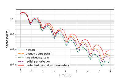
Figure 1: Norm of pendulum state over time starting at a fixed initial condition, for nominal and perturbed trajectories perturbed as described in Section 4.

We consider the following four classes of perturbed trajectories:

1. $\dot{x}=f(x)+\varepsilon\frac{\left\|x\right\|_{2}}{\left\|\nabla V_{\mathrm{adv}}(x)\right\|_{2}}\nabla V_{\mathrm{adv}}(x)$, analogous to the adversarial training process,

2. $\dot{x}=f(x)+\varepsilon x$, which is a Lipschitz adversary that aims to greedily maximize $\left\|x(t)\right\|_{2}^{2}$ at any given time $t$,

3. the dynamics resulting from using the linearization of the damped pendulum at the origin to generate the trajectories, and

4. the dynamics resulting from setting $\tilde{m}=\tilde{\ell}=1.1$ instead of $m=\ell=1$.

The perturbation class 1 acts in the direction $\nabla V_{\mathrm{adv}}$, and thus the perturbed trajectories are tuned to degrade the performance of $V_{\mathrm{adv}}$. Additionally, the perturbation classes 3 and 4 can be viewed as instances of the sim-to-real gap, where there are model discrepancies between training and test.

Figure 2 plots the resulting Lyapunov decrease satisfaction rates for each type of perturbation. We observe that for each type of perturbation, the nominal certificate $V_{\mathrm{nom}}$ fails to certify any trajectories when $\eta=0.4$. In contrast, the robust certificate $V_{\mathrm{adv}}$ certifies all trajectories for decrease rates $\eta=0.4$. We further observe that the robust certificate is also able to certify faster decrease rates as well. Finally, we note that the trajectories resulting from perturbed pendulum parameters (perturbation class 4) actually cause the system to be more unstable than the greedy perturbations (perturbation class 1) used during training (see Figure 1). Nevertheless, the robust certificate $V_{\mathrm{adv}}$ is able to certify stability for a large range of $\eta$.

5 Conclusion

Motivated by bridging the sim-to-real gap, we proposed and analyzed an approach to learning adversarially robust Lyapunov certificates. We showed that for systems that enjoy exponential incremental input-to-state stability, stability certificate functions that are robust to norm-bounded and Lipschitz adversarial perturbations to the system dynamics can be learned with negligible statistical overhead as compared to the nominal case. Future research directions include exploring the statistical tradeoffs occurring from progressively weaker notions of stability (e.g., incremental gain stability as defined in Tu et al. [43]), providing approximation guarantees for the adversarial training algorithm proposed in Section 4, and extending our results to provide statistical guarantees for policies synthesized from robust certificate functions [19, 38].

                                                                                                                                                                                                                                                                   

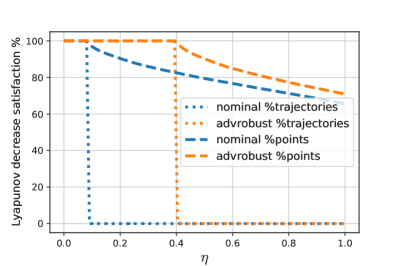
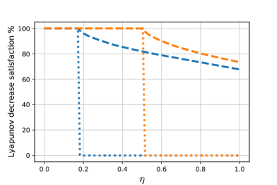
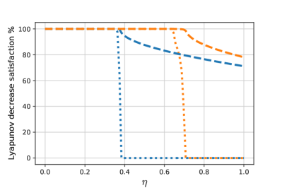
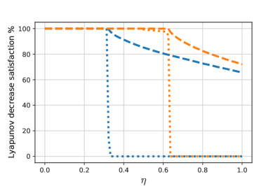
Figure 2: Satisfaction rate of the Lyapunov decrease condition versus the exponential rate parameter $\eta$ of nominal and adversarially trained certificates $V_{\mathrm{nom}}$ and $V_{\mathrm{adv}}$ for four classes of perturbed trajectories. The percentage of trajectories and of total points satisfying the Lyapunov decrease condition for $V_{\mathrm{nom}}$ and $V_{\mathrm{adv}}$ are shown. Both $V_{\mathrm{nom}}$ and $V_{\mathrm{adv}}$ were trained with $\eta=0.4$. Trajectories were generated by rolling out a fixed set of $1000$ initial conditions sampled from $\mathrm{Unif}\mathopen{}\left([-2,2]^{2}\right)\mathclose{}$. Upper left: dynamics generated from gradient ascent on the adversarial certificate $V_{\mathrm{adv}}$, $\dot{x}=f(x)+\varepsilon\frac{\left\|x\right\|}{\left\|\nabla{V_{\mathrm{adv}}}\right\|}\nabla V_{\mathrm{adv}}$. Upper right: dynamics generated from a radial perturbation, $\dot{x}=f(x)+\varepsilon x$. Lower left: dynamics generated from system linearized at origin, $\dot{x}=J_{(0,0)}x$. Lower right: dynamics generated from perturbing the pendulum parameters, $\tilde{m}=1.1$, $\tilde{\ell}=1.1$.

Appendix A Proofs for Section 3

A.1 Proof of Lemma 2

The result follows by observing

$$\tilde{h}(\xi,V_{1})-\tilde{h}(\xi,V_{2}) :=\sup_{\tilde{\varphi}\in\Delta_{\varepsilon}}\sup_{t\in\mathcal{T}}\left\langle\nabla V_{1}(\tilde{\varphi}_{t}(\xi)),f(\tilde{\varphi}_{t}(\xi))+\delta_{t}\right\rangle+\eta V_{1}(\tilde{\varphi}_{t}(\xi))-\nu$$

$$\quad-\sup_{\tilde{\varphi}\in\Delta_{\varepsilon}}\mathopen{}\left(\left\langle\nabla V_{2}(\tilde{\varphi}_{t}(\xi)),f(\tilde{\varphi}_{t}(\xi))+\delta_{t}\right\rangle+\eta V_{2}(\tilde{\varphi}_{t}(\xi))-\nu\right)\mathclose{}$$

$$\leqslant\sup_{\tilde{\varphi}\in\Delta_{\varepsilon}}\sup_{t\in\mathcal{T}}\left\langle\nabla V_{1}(\tilde{\varphi}_{t}(\xi)),f(\tilde{\varphi}_{t}(\xi))+\delta_{t}\right\rangle+\eta V_{1}(\tilde{\varphi}_{t}(\xi))$$

$$\quad-\mathopen{}\left(\left\langle\nabla V_{2}(\tilde{\varphi}_{t}(\xi)),f(\tilde{\varphi}_{t}(\xi))+\delta_{t}\right\rangle+\eta V_{2}(\tilde{\varphi}_{t}(\xi))\right)\mathclose{}$$

$$\leqslant L_{h}\left\|V_{1}-V_{2}\right\|_{\mathcal{V}}+\left\langle\nabla V_{1}(\tilde{\varphi}_{t}(\xi))-\nabla V_{2}(\tilde{\varphi}_{t}(\xi)),\delta_{t}\right\rangle$$

$$\leqslant L_{h}\left\|V_{1}-V_{2}\right\|_{\mathcal{V}}+\left\|\nabla V_{1}(\tilde{\varphi}_{t}(\xi))-\nabla V_{2}(\tilde{\varphi}_{t}(\xi))\right\|_{2}\left\|\delta_{t}\right\|_{2}$$

$$\leqslant\mathopen{}\left(L_{h}+B_{\delta}\right)\mathclose{}\left\|V_{1}-V_{2}\right\|_{\mathcal{V}}.$$

Swapping the roles of $V_{1}$ and $V_{2}$ completes the proof.

A.2 Proof of Lemma 3

We first state a few definitions. Let $\mathsf{Sym}_{\geqslant 0}^{n\times n}$ denote the space of $n\times n$ real-valued positive semi-definite matrices. Given a Riemannian metric $M:\mathbb{R}^{n}\rightarrow\mathsf{Sym}_{\geqslant 0}^{n\times n}$, the geodesic distance associated with $M$ is:

$$d_{M}(x,y):=\inf_{\gamma\in\Gamma(x,y)}\int_{0}^{1}\sqrt{\gamma^{\prime}(s)\operatorname{{}^{\top}}M(\gamma(s))\gamma^{\prime}(s)}ds,$$

where $\Gamma(x,y)$ denotes the set of smooth curves $\gamma$ with endpoints at $\gamma(0)=x$ and $\gamma(1)=y$.

Now, given a time-varying metric $M:\mathbb{R}^{n}\times\mathbb{R}\rightarrow\mathsf{Sym}_{\geqslant 0}^{n\times n}$, a function $f(x,t)$ is said to be contracting in the metric $M(x,t)$ at rate $\lambda$ if for all $x$ and $t$:

$$\frac{\partial f}{\partial x}(x,t)\operatorname{{}^{\top}}M(x,t)+M(x,t)\frac{\partial f}{\partial x}(x,t)+\dot{M}(x,t)\preccurlyeq-2\lambda M(x,t).$$

Proposition 1.

Consider two nonlinear systems

$$\dot{x}_{p} =f(x_{p},t)+d(x_{p},t),$$

$$\dot{x} =f(x,t),$$

where $f(x,t)$ is contracting in the metric $M(x,t)$. Then the geodesic distance $d_{M(\cdot,t)}(x_{p}(t),x(t))$ satisfies the differential inequality

$$\frac{d}{dt}d_{M(\cdot,t)}(x_{p}(t),x(t))\leqslant-\lambda d_{M(\cdot,t)}(x_{p}(t),x(t))+\left\|\Theta(x_{p}(t),t)d(x_{p}(t),t)\right\|_{2},$$

where $M(x,t)=\Theta(x,t)\operatorname{{}^{\top}}\Theta(x,t)$.

Proof.

Consider a geodesic $\gamma_{t}(s):[0,1]\rightarrow\mathbb{R}^{n}$ from $x_{p}(t)$ to $x(t)$ so that $\gamma_{t}(0)=x_{p}(t)$ and $\gamma_{t}(1)=x(t)$, and let $\gamma_{t}^{\prime}$ denote the derivative of $\gamma_{t}$ with respect to its argument. Observe that the Riemannian energy is $E(\gamma_{t})=d_{M}(x_{p}(t),x(t))^{2}$, and hence $\dot{E}(\gamma_{t})=2d_{M}(x_{p}(t),x(t))\left(\frac{d}{dt}d_{M}(x_{p}(t),x(t))\right)$. From the formula for the first variation of the Riemannian energy for a minimizing geodesic,

$$\dot{E}(\gamma_{t})=2\left\langle\gamma_{t}^{\prime}(s),\dot{\gamma}_{t}(s)\right\rangle|_{s=0}^{s=1}+2\frac{\partial E}{\partial t},$$

where $\dot{\gamma}_{t}$ denotes the time derivative of $\gamma_{t}$ along the flow of $x_{p}(t)$, and $\left\langle\cdot,\cdot\right\rangle$ denotes the Riemannian inner product. Note that while the functional form of $\gamma_{t}(s)$ is unknown, the values of its time derivative at the endpoints are fixed to be $\dot{x}_{p}$ and $\dot{x}$ for $s=0$ and $s=1$, respectively. From this, we find that

$$\dot{E}(\gamma_{t}) =2\left\langle\gamma^{\prime}_{t}(1),f(x)\right\rangle-2\left\langle\gamma^{\prime}_{t}(0),f(x_{p})+d(x_{p},t)\right\rangle+2\frac{\partial E}{\partial t}$$

$$\leqslant-2\lambda E(\gamma_{t})-2\left\langle\gamma^{\prime}_{t}(0),d(x_{p},t)\right\rangle,$$

where the inequality stems from contraction of the nominal dynamics $f(x,t)$. This relation then implies the decrease condition

$$\frac{d}{dt}d_{M(\cdot,t)}(x_{p}(t),x(t)) \leqslant-\lambda d_{M(\cdot,t)}(x_{p}(t),x(t))-\frac{1}{d_{M(\cdot,t)}(x_{p}(t),x(t))}\gamma^{\prime}_{t}(0)\operatorname{{}^{\top}}\Theta(x_{p})\operatorname{{}^{\top}}\Theta(x_{p})d(x_{p},t),$$

$$\leqslant-\lambda d_{M(\cdot,t)}(x_{p}(t),x(t))+\frac{\left\|\Theta(x_{p},t)\gamma^{\prime}_{t}(0)\right\|_{2}}{d_{M(\cdot,t)}(x_{p}(t),x(t))}\left\|\Theta(x_{p},t)d(x_{p},t)\right\|_{2}.$$

To complete the proof, observe that geodesics have constant energy, so that $\left\|\Theta(x_{p},t)\gamma^{\prime}_{t}(0)\right\|_{2}=d_{M(\cdot,t)}(x_{p}(t),x(t))$. ∎

We can now prove Lemma 3. By Proposition 1 and the assumption that $M(x,t)\preccurlyeq LI$,

$$\frac{d}{dt}d_{M(\cdot,t)}(x_{p}(t),x(t)) \leqslant-\lambda d_{M(\cdot,t)}(x_{p}(t),x(t))+\left\|\Theta(x(t),t)d(x(t),t)\right\|_{2}$$

$$\leqslant-\lambda d_{M(\cdot,t)}(x_{p}(t),x(t))+\sqrt{L}\left\|d(x_{p}(t),t)\right\|_{2}.$$

By the comparison lemma,

$$d_{M(\cdot,t)}(x_{p}(t),x(t))\leqslant d_{M(\cdot,0)}(x_{p}(0),x(0))e^{-\lambda t}+\sqrt{L}\int_{0}^{t}e^{-\lambda(t-s)}\left\|d(x_{p}(s),s)\right\|_{2}ds.$$

Next, by the assumption that $\mu I\preccurlyeq M(x,t)\preccurlyeq LI$, it is not hard to see (see e.g. Proposition D.2 of Boffi et al. [5]) that for all $x,y,t$,

$$\sqrt{\mu}\left\|x-y\right\|_{2}\leqslant d_{M(\cdot,t)}(x,y)\leqslant\sqrt{L}\left\|x-y\right\|_{2}$$

Combining these inequalities, we have:

$$\sqrt{\mu}\left\|x_{p}(t)-x(t)\right\|_{2}\leqslant\sqrt{L}\left\|x_{p}(0)-x(0)\right\|_{2}e^{-\lambda t}+\sqrt{L}\int_{0}^{t}e^{-\lambda(t-s)}\left\|d(x_{p}(s),s)\right\|_{2}ds.$$

The claim now follows by dividing both sides by $\sqrt{\mu}$.

A.3 Proof of Theorem 1

We observe that for an arbitrary perturbation tube $\Delta(\xi)$

$$\tilde{h}(\xi,V)-h(\xi,V) =\sup_{\tilde{\varphi}\in\Delta(\xi)}\sup_{t\in\mathcal{T}}\left\langle\nabla V(\tilde{\varphi}_{t}(\xi)),f(\tilde{\varphi}_{t}(\xi))+\delta_{t}\right\rangle+\eta V(\tilde{\varphi}_{t}(\xi))-\nu$$

$$\quad-\sup_{t\in\mathcal{T}}\mathopen{}\left(\left\langle\nabla V(\varphi_{t}(\xi)),f(\varphi_{t}(\xi))\right\rangle+\eta V(\varphi_{t}(\xi))\right)\mathclose{}$$

$$\leqslant\sup_{\tilde{\varphi}\in\Delta(\xi)}\sup_{t\in\mathcal{T}}\left\langle\nabla V(\tilde{\varphi}_{t}(\xi)),f(\tilde{\varphi}_{t}(\xi))+\delta_{t}\right\rangle+\eta V(\tilde{\varphi}_{t}(\xi))-\nu$$

$$\quad-\mathopen{}\left(\left\langle\nabla V(\varphi_{t}(\xi)),f(\varphi_{t}(\xi))\right\rangle+\eta V(\varphi_{t}(\xi))\right)\mathclose{}$$

$$\leqslant\sup_{\tilde{\varphi}\in\Delta(\xi)}\sup_{t\in\mathcal{T}}\;(L_{\nabla V}+\eta L_{V})\left\|\tilde{\varphi}_{t}(\xi)-\varphi_{t}(\xi)\right\|_{2}+B_{\nabla V}\left\|\delta_{t}\right\|_{2}-\nu,$$

and thus

$${\mathopen{}\left|\tilde{h}(\xi,V)-h(\xi,V)\right|\mathclose{}}\leqslant\sup_{\tilde{\varphi}\in\Delta(\xi)}\sup_{t\in\mathcal{T}}\;(L_{\nabla V}+\eta L_{V})\left\|\tilde{\varphi}_{t}(\xi)-\varphi_{t}(\xi)\right\|_{2}+B_{\nabla V}\left\|\delta_{t}\right\|_{2}+\nu$$ (19)

• Norm-bounded Adversary $\Delta_{\varepsilon}^{u}$: from E$\delta$ISS, we know that the deviation can be bounded by:

  $$\left\|\varphi_{t}-\tilde{\varphi}_{t}\right\|_{2} \leqslant\beta\left\|\varphi_{0}-\tilde{\varphi}_{0}\right\|e^{-\rho t}+\gamma\int_{0}^{t}e^{-\rho(t-s)}\left\|\delta_{s}\right\|_{2}\,ds$$

  $$\leqslant\gamma\varepsilon\int_{0}^{t}e^{-\rho(t-s)}\;ds$$

  $$\leqslant\gamma\varepsilon\rho^{-1}.$$

  Plugging this back into (19), we get

  $${\mathopen{}\left|\tilde{h}(\xi,V)-h(\xi,V)\right|\mathclose{}} \leqslant\mathopen{}\left(L_{\nabla V}+\eta L_{V}\right)\mathclose{}\gamma\varepsilon\rho^{-1}+B_{\nabla V}\varepsilon+\nu.$$

  Applying (12) yields the desired result.

• Lipschitz Adversary $\Delta_{\varepsilon}^{x}$: from E$\delta$ISS, we can bound the deviation by:

  $$\left\|\varphi_{t}-\tilde{\varphi}_{t}\right\|_{2} \leqslant\beta\left\|\varphi_{0}-\tilde{\varphi}_{0}\right\|e^{-\rho t}+\gamma\int_{0}^{t}e^{-\rho(t-s)}\left\|\delta(\tilde{\varphi}_{s})\right\|_{2}\,ds$$

  $$\leqslant\gamma\varepsilon\int_{0}^{t}e^{-\rho(t-s)}\left\|\tilde{\varphi}_{s}\right\|_{2}\;ds$$

  $$\leqslant\gamma\varepsilon\int_{0}^{t}e^{-\rho(t-s)}\mathopen{}\left(\left\|\varphi_{s}-\tilde{\varphi}_{s}\right\|_{2}+\left\|\varphi_{s}\right\|_{2}\right)\mathclose{}\;ds$$

  $$\leqslant\gamma\varepsilon\int_{0}^{t}e^{-\rho(t-s)}\left\|\varphi_{s}-\tilde{\varphi}_{s}\right\|_{2}\;ds+\gamma\varepsilon\int_{0}^{t}e^{-\rho(t-s)}\beta\left\|\xi\right\|_{2}e^{-\rho s}\;ds$$

  $$=\gamma\varepsilon\int_{0}^{t}e^{-\rho(t-s)}\left\|\varphi_{s}-\tilde{\varphi}_{s}\right\|_{2}\;ds+\gamma\varepsilon\beta\left\|\xi\right\|_{2}te^{-\rho t}.$$

  Taking the supremum over $t$ on both sides, we have

  $$\sup_{t\in\mathcal{T}}\left\|\varphi_{t}-\tilde{\varphi}_{t}\right\|_{2} \leqslant\sup_{t\in\mathcal{T}}\gamma\varepsilon\int_{0}^{t}e^{-\rho(t-s)}\left\|\varphi_{s}-\tilde{\varphi}_{s}\right\|_{2}\;ds+\gamma\varepsilon\beta\left\|\xi\right\|_{2}te^{-\rho t}$$

  $$\leqslant\gamma\varepsilon\sup_{t\in\mathcal{T}}\int_{0}^{t}e^{-\rho(t-s)}\sup_{s\in\mathcal{T}}\left\|\varphi_{s}-\tilde{\varphi}_{s}\right\|_{2}\;ds+\sup_{t\in\mathcal{T}}\gamma\varepsilon\beta\left\|\xi\right\|_{2}te^{-\rho t}$$

  $$\leqslant\gamma\varepsilon\rho^{-1}\sup_{s\in\mathcal{T}}\left\|\varphi_{s}-\tilde{\varphi}_{s}\right\|_{2}+\gamma\varepsilon\rho^{-1}\beta\left\|\xi\right\|_{2}e^{-1},$$

  where the second term in the last line comes from optimizing $\max_{t}te^{-\rho t}$, which attains its maximum $\frac{1}{\rho e}$ at $t=1/\rho$. Since by assumption, $\frac{\gamma\varepsilon}{\rho}<1$, we have

  $$\sup_{t\in\mathcal{T}}\left\|\varphi_{t}-\tilde{\varphi}_{t}\right\|_{2} \leqslant\frac{\gamma\varepsilon\rho^{-1}}{1-\gamma\varepsilon\rho^{-1}}\beta e^{-1}\left\|\xi\right\|_{2}.$$

  Plugging this into (19), we get

  $${\mathopen{}\left|\tilde{h}(\xi,V)-h(\xi,V)\right|\mathclose{}} \leqslant\sup_{\tilde{\varphi}\in\Delta_{\varepsilon}(\xi)}\sup_{t\in\mathcal{T}}\;\mathopen{}\left(L_{\nabla V}+\eta L_{V}\right)\mathclose{}\left\|\tilde{\varphi}_{t}(\xi)-\varphi_{t}(\xi)\right\|_{2}+B_{\nabla V}\left\|\delta(\tilde{\varphi}_{t}(\xi))\right\|_{2}+\nu$$

  $$\leqslant\sup_{\tilde{\varphi}\in\Delta_{\varepsilon}(\xi)}\sup_{t\in\mathcal{T}}\;\mathopen{}\left(L_{\nabla V}+\eta L_{V}\right)\mathclose{}\left\|\tilde{\varphi}_{t}-\varphi_{t}\right\|_{2}+B_{\nabla V}\varepsilon\mathopen{}\left(\left\|\varphi_{t}-\tilde{\varphi}_{t}\right\|_{2}+\left\|\tilde{\varphi}_{t}\right\|_{2}\right)\mathclose{}+\nu$$

  $$\leqslant\mathopen{}\left(L_{\nabla V}+\eta L_{V}+B_{\nabla V}\varepsilon\right)\mathclose{}\frac{\gamma\varepsilon\rho^{-1}}{1-\gamma\varepsilon\rho^{-1}}\beta e^{-1}\left\|\xi\right\|_{2}+\sup_{t}B_{\nabla V}\beta\varepsilon\left\|\xi\right\|_{2}e^{-\rho t}+\nu$$

  $$\leqslant\mathopen{}\left[\mathopen{}\left(L_{\nabla V}+\eta L_{V}+B_{\nabla V}\varepsilon\right)\mathclose{}\frac{\gamma\varepsilon\rho^{-1}}{1-\gamma\varepsilon\rho^{-1}}e^{-1}+B_{\nabla V}\right]\mathclose{}\beta\varepsilon\left\|\xi\right\|_{2}+\nu.$$

  Applying (12) yields the desired result.

• Combined Adversary $\Delta_{\varepsilon_{x},\varepsilon_{u}}^{x,u}$: proof follows similarly to the Lipschitz adversary case. Using E$\delta$ISS, we have

  $$\left\|\varphi_{t}-\tilde{\varphi}_{t}\right\|_{2} \leqslant\beta\left\|\varphi_{0}-\tilde{\varphi}_{0}\right\|e^{-\rho t}+\gamma\int_{0}^{t}e^{-\rho(t-s)}\left\|\delta(\tilde{\varphi}_{s})+\delta_{t}\right\|_{2}\,ds$$

  $$\leqslant\gamma\varepsilon_{x}\int_{0}^{t}e^{-\rho(t-s)}\left\|\tilde{\varphi}_{s}\right\|_{2}\;ds+\gamma\varepsilon_{u}\rho^{-1}$$

  $$=\gamma\varepsilon_{x}\int_{0}^{t}e^{-\rho(t-s)}\left\|\varphi_{s}-\tilde{\varphi}_{s}\right\|_{2}\;ds+\gamma\varepsilon_{x}\beta\left\|\xi\right\|_{2}te^{-\rho t}+\gamma\varepsilon_{u}\rho^{-1}.$$

  Since $\gamma\varepsilon_{x}<\rho$, we take the supremum of both sides and shift terms around to get

  $$\sup_{t\in\mathcal{T}}\left\|\varphi_{t}-\tilde{\varphi}_{t}\right\|_{2} \leqslant\frac{\gamma\varepsilon_{u}\rho^{-1}+\gamma\varepsilon_{x}\rho^{-1}\beta e^{-1}\left\|\xi\right\|_{2}}{1-\gamma\varepsilon_{x}\rho^{-1}},$$

  and thus plugging into (19), we get

  $${\mathopen{}\left|\tilde{h}(\xi,V)-h(\xi,V)\right|\mathclose{}} \leqslant\mathopen{}\left(L_{\nabla V}+\eta L_{V}+B_{\nabla V}\varepsilon_{x}\right)\mathclose{}\frac{\gamma\varepsilon_{u}\rho^{-1}+\gamma\varepsilon_{x}\rho^{-1}e^{-1}\beta\varepsilon_{x}\left\|\xi\right\|_{2}}{1-\gamma\varepsilon_{x}\rho^{-1}}$$

  $$\quad+B_{\nabla V}\beta\varepsilon_{x}\left\|\xi\right\|_{2}+B_{\nabla V}\varepsilon_{u}+\nu.$$

  Applying (12) yields the desired result.

Appendix B Adversarially Robust Certificates in Discrete Time

In the discrete time setting, we consider the system $x_{t+1}=f(x_{t})$. Like in the continuous time case, $f$ is continuous and unknown, the state $x\in\mathbb{R}^{p}$ is fully observed, the initial conditions $\xi$ are drawn from some compact set $\mathcal{X}$, and $\varphi_{t}(\xi)$ denotes the map to the state at time $t$ given initial condition $\xi$. Given a candidate Lyapunov function $V$, we define the nominal and adversarial (exponential) Lyapunov decrease conditions as:

$$h(\xi,V) =\max_{t\leqslant T}V\mathopen{}\left(\varphi_{t+1}(\xi)\right)\mathclose{}-\eta^{2}V\mathopen{}\left(\varphi_{t}(\xi)\right)\mathclose{}$$

$$\tilde{h}_{\nu}(\xi,V) =\max_{\tilde{\varphi}\in\Delta_{\varepsilon}(\xi)}\max_{t\leqslant T}V\mathopen{}\left(\tilde{\varphi}_{t+1}(\xi)\right)\mathclose{}-\eta^{2}V\mathopen{}\left(\tilde{\varphi}_{t}(\xi)\right)\mathclose{}-\nu,\quad\nu\geqslant 0,$$

where $0<\eta<1$, as well as the corresponding loss classes $\mathcal{H}$ and $\tilde{\mathcal{H}}$. The stability certification problem can be posed as the following feasibility problem

$$\mathrm{Find}_{V\in\mathcal{V}}\;\mathrm{s.t.}\;\;\tilde{h}_{\nu}(\xi,V)\leqslant-\tau,\quad i=1,\dots,n.$$ (20)

We make the following assumptions.

Assumption 3 (Discrete-time stability in the sense of Lyapunov).

Fix a perturbation set $\Delta(\cdot)$. There exists a compact set $S\subseteq\mathbb{R}^{p}$ such that $\tilde{\varphi}_{t}(\xi)\in S$ for all $\xi\in\mathcal{X}$, $t\leqslant T$, and $\tilde{\varphi}_{t}(\xi)\in\Delta(\xi)$.

Assumption 4 (Regularity of $\mathcal{V}$).

There exist a constant $L_{V}$ such that for every $V\in\mathcal{V}$, the map $x\to V(x)$ over $x\in S$ is $L_{V}$-Lipschitz.

Under Assumptions 3 and 4, and the continuity of the dynamics $f(x)$, there exist constants $B_{V}$ and $B_{\tilde{h}}$ such that

$$\sup_{V\in\mathcal{V}}\sup_{x\in S}{\mathopen{}\left|V(x)\right|\mathclose{}}\leqslant B_{V},\;\sup_{V\in\mathcal{V}}\sup_{\xi\in\mathcal{X}}{\mathopen{}\left|\tilde{h}(\xi,V)\right|\mathclose{}}\leqslant B_{\tilde{h}}.$$

Finally, let $\left\|V\right\|_{\mathcal{V}}:=\sup_{x\in S}{\mathopen{}\left|V(x)\right|\mathclose{}}$ denote the supremum norm on the space $\mathcal{V}$. Under Assumptions 3 and 4, and the discrete time definition of $\tilde{h}$, Lemma 1 holds in precisely the same form, such that we once again need only to bound the Rademacher complexity of the adversarial loss class. We now prove the discrete-time variant of the adversary-agnostic Rademacher complexity bound.

Lemma 4 (Discrete-time analogue of Lemma 2).

Suppose that Assumptions 3 and 4 hold. Let $L_{h}$ denote any constant such that ${\mathopen{}\left|h(\xi,V_{1})-h(\xi,V_{2})\right|\mathclose{}}\leqslant L_{h}\left\|V_{1}-V_{2}\right\|_{\mathcal{V}}$ for all $\xi\in X$ and $V_{1},V_{2}\in\mathcal{V}$. Then, $L_{\tilde{h}}\leqslant L_{h}+2$.

Proof.

Writing out $\tilde{h}(\xi,V_{1})-\tilde{h}(\xi,V_{2})$, for arbitrary $\xi$, $V_{1}$, $V_{2}$, we have:

$$\tilde{h}(\xi,V_{1})-\tilde{h}(\xi,V_{2}) =\max_{\tilde{\varphi}\in\Delta(\xi)}\max_{t\leqslant T}V_{1}(\tilde{\varphi}_{t+1})-\eta^{2}V_{1}(\tilde{\varphi}_{t})-\max_{\tilde{\varphi}\in\Delta(\xi)}\max_{t\leqslant T}\mathopen{}\left(V_{2}(\tilde{\varphi}_{t+1})-\eta^{2}V_{2}(\tilde{\varphi}_{t})\right)\mathclose{}$$

$$\leqslant\max_{\tilde{\varphi}\in\Delta(\xi)}\max_{t\leqslant T}V_{1}(\tilde{\varphi}_{t+1})-\eta^{2}V_{1}(\tilde{\varphi}_{t})-\mathopen{}\left(V_{2}(\tilde{\varphi}_{t+1})-\eta^{2}V_{2}(\tilde{\varphi}_{t})\right)\mathclose{}.$$

For any time $t$, we have

$$V_{1}(\tilde{\varphi}_{t+1})-\eta^{2}V_{1}(\tilde{\varphi}_{t})-\mathopen{}\left(V_{2}(\tilde{\varphi}_{t+1})-\eta^{2}V_{2}(\tilde{\varphi}_{t})\right)\mathclose{} =V_{1}(f(\tilde{\varphi}_{t}))-\eta^{2}V_{1}(\tilde{\varphi}_{t})-\mathopen{}\left(V_{2}(f(\tilde{\varphi}_{t}))-\eta^{2}V_{2}(\tilde{\varphi}_{t})\right)\mathclose{}$$

$$\quad+\mathopen{}\left(V_{1}(\tilde{\varphi}_{t+1})-V_{2}(\tilde{\varphi}_{t+1})\right)\mathclose{}$$

$$\quad-\mathopen{}\left(V_{1}(f(\tilde{\varphi}_{t}))-V_{2}(f(\tilde{\varphi}_{t}))\right)\mathclose{}$$

$$\leqslant{\mathopen{}\left|h(\xi,V_{1})-h(\xi,V_{2})\right|\mathclose{}}+2\sup_{x\in S}{\mathopen{}\left|V_{1}(x)-V_{2}(x)\right|\mathclose{}}$$

$$\leqslant L_{h}\left\|V_{1}-V_{2}\right\|_{\mathcal{V}}+2\left\|V_{1}-V_{2}\right\|_{\mathcal{V}},$$

where added and subtracted $V_{1}(f(\tilde{\varphi}_{t}))$ and $V_{2}(f(\tilde{\varphi}_{t}))$, and used Assumption 1 to bound the leftover terms using the definition of $\left\|\cdot\right\|_{\mathcal{V}}$. The argument is symmetric for $V_{1},V_{2}$, so we have

$${\mathopen{}\left|\tilde{h}(\xi,V_{1})-\tilde{h}(\xi,V_{2})\right|\mathclose{}}\leqslant(L_{h}+2)\left\|V_{1}-V_{2}\right\|_{\mathcal{V}},$$

for all $\xi\in X$ and $V_{1},V_{2}\in\mathcal{V}$. ∎

We note this is at first glance a better bound than the continuous-time version. This can be attributed to the fact that Assumption 3 is at face value more restrictive than its continuous-time analogue Assumption 1, since it implicitly enforces a norm-constraint on $\delta_{t}$ such that it cannot push $x_{t}$ out of the compact set $S$, which is a property independent of the certificate $V$. On the other hand, Assumption 1 does not immediately enforce a norm-constraint on $\delta_{t}$–the implicit constraint depends on the choice of $V$, where $\delta_{t}$ cannot render optimization problem (9) infeasible. As Assumption 3 is in a sense more restrictive than Assumption 1, the bound we get is stronger.

We now re-introduce the norm-bounded, Lipschitz, and combined adversarial trajectory tubes in discrete time:

$$\Delta^{u}_{\varepsilon}(\xi):=\mathopen{}\left\{\tilde{\varphi}:\tilde{\varphi}_{t+1}=f(\tilde{\varphi}_{t})+\delta_{t},\;\tilde{\varphi}_{0}=\xi,\;\left\|\delta_{t}\right\|_{2}\leqslant\varepsilon\right\}\mathclose{}$$ (21)

$$\Delta^{x}_{\varepsilon}(\xi):=\mathopen{}\left\{\tilde{\varphi}:\tilde{\varphi}_{t+1}=f(\tilde{\varphi}_{t})+\delta(\tilde{\varphi}_{t}),\;\tilde{\varphi}_{0}=\xi,\;\left\|\delta(\tilde{\varphi}_{t})\right\|_{2}\leqslant\varepsilon\left\|\tilde{\varphi}_{t}\right\|_{2}\right\}\mathclose{}$$ (22)

$$\Delta^{x,u}_{\varepsilon_{x},\varepsilon_{u}}(\xi):=\mathopen{}\left\{\tilde{\varphi}:\tilde{\varphi}_{t+1}=f(\tilde{\varphi}_{t})+\delta^{x}(\tilde{\varphi}_{t})+\delta^{u}_{t},\;\tilde{\varphi}_{0}=\xi,\;\left\|\delta^{x}(\tilde{\varphi}_{t})\right\|_{2}\leqslant\varepsilon_{x}\left\|\tilde{\varphi}_{t}\right\|_{2},\;\left\|\delta^{u}_{t}\right\|_{2}\leqslant\varepsilon_{u}\right\}\mathclose{}.$$ (23)

Accordingly, we introduce $(\beta,\rho,\gamma)$-E$\delta$ISS in discrete time.

Definition 2 (Discrete-time $(\beta,\rho,\gamma)$-E$\delta$ISS).

Let $\beta,\gamma>0$ be positive constants and $\rho\in(0,1)$. A discrete-time dynamical system $f(x,t)$ is $(\beta,\rho,\gamma)$-exponential-incrementally-input-to-state stable if for every pair of initial conditions $(x_{0},y_{0})$ and signal $u_{t}$ (which can depend causally on $x,y$), the trajectories $x_{t+1}=f(x_{t},t)$ and $y_{t+1}=f(y_{t},t)+u_{t}$ satisfy for all $t\geqslant 0$:

$$\left\|x_{t}-y_{t}\right\|_{2}\leqslant\beta\rho^{t}\left\|x_{0}-y_{0}\right\|_{2}+\gamma\sum_{k=0}^{t-1}\rho^{t-1-k}\left\|u_{k}\right\|_{2}.$$ (24)

As mentioned earlier in this paper, Proposition 5.3 of [5] gives that a discrete-time system contracting with respect to some metric is $(\beta,\rho,\gamma)$-E$\delta$ISS. We are now ready to provide the discrete-time analogues to the adversarial Rademacher complexities provided in Theorem 1.

Theorem 2 (Discrete-time analogue to Theorem 1).

Put $B_{X}:=\sup_{\xi\in\mathcal{X}}\left\|\xi\right\|_{2}$, let Assumption 4 hold, and assume that the nominal discrete-time system $f(x)$ is $(\beta,\rho,\gamma)$-E$\delta$ISS. Then for

• adversarial trajectories drawn from the norm-bounded tube $\Delta^{u}_{\varepsilon}(\xi)$ defined in (21), Assumption 3 holds and

  $$\mathcal{R}_{n}(\tilde{\mathcal{H}}) \leqslant\mathcal{R}_{n}(\mathcal{H})+\mathopen{}\left[(1+\eta^{2})L_{V}\frac{\gamma\varepsilon}{1-\rho}+\nu\right]\mathclose{}\frac{1}{\sqrt{n}},$$ (25)

• adversarial trajectories drawn from the Lipschitz tube $\Delta^{x}_{\varepsilon}(\xi)$ defined in (22), if $\varepsilon>0$ is small enough such that $\rho+\gamma\varepsilon<1$, then Assumption 3 holds and

  $$\mathcal{R}_{n}(\tilde{\mathcal{H}}) \leqslant\mathcal{R}_{n}(\mathcal{H})+\mathopen{}\left[L_{V}\beta B_{X}(\rho+\gamma\varepsilon+\eta^{2})+\nu\right]\mathclose{}\frac{1}{\sqrt{n}},$$ (26)

• adversarial trajectories drawn from the combined tube $\Delta^{x,u}_{\varepsilon_{x},\varepsilon_{u}}$ defined in (23), if $\varepsilon_{x}>0$ is small enough such that $\rho+\gamma\varepsilon_{x}<1$, then Assumption 3 holds and

  $$\mathcal{R}_{n}(\tilde{\mathcal{H}}) \leqslant\mathcal{R}_{n}(\mathcal{H})+\bigg{[}(1+\eta^{2})L_{V}\mathopen{}\left(\frac{1-\rho}{1-(\rho+\gamma\varepsilon_{x})}\frac{\gamma\beta B_{X}\varepsilon_{x}}{e\rho\log\mathopen{}\left(\rho^{-1}\right)\mathclose{}}+\frac{\gamma\varepsilon_{u}}{1-\rho}\right)\mathclose{}+\nu\bigg{]}\frac{1}{\sqrt{n}}.$$ (27)

We note that the necessary condition that $\rho+\gamma\varepsilon<1$ for the Lipschitz and combined adversaries is nicely analogous to the continuous-time case where we needed $\gamma\varepsilon<\rho$; in both cases, the adversary cannot be powerful enough to de-stabilize the system. One can consider the scalar system $x_{t+1}=\rho x_{t}$, $0<\rho<1$ and the adversary $\delta(x)=\varepsilon x$ to see why this condition cannot be loosened in general. We now provide the proof to Theorem 2.

Proof.

We observe that for an arbitrary perturbation tube $\Delta(\xi)$

$$\tilde{h}(\xi,V)-h(\xi,V) =\sup_{\tilde{\varphi}\in\Delta(\xi)}\sup_{t\leqslant T}\;V(\tilde{\varphi}_{t+1})-\eta^{2}V(\tilde{\varphi}_{t})-\nu-\sup_{t\leqslant T}\mathopen{}\left(V(\varphi_{t+1})-\eta^{2}V(\varphi_{t})\right)\mathclose{}$$

$$\leqslant\sup_{\tilde{\varphi}\in\Delta(\xi)}\sup_{t\leqslant T}\;V(\tilde{\varphi}_{t+1})-V(\varphi_{t+1})-\eta^{2}\mathopen{}\left(V(\tilde{\varphi}_{t})-V(\varphi_{t})\right)\mathclose{}-\nu$$

$$\leqslant\sup_{\tilde{\varphi}\in\Delta(\xi)}\sup_{t\leqslant T}\;(1+\eta^{2})L_{V}\left\|\tilde{\varphi}_{t}-\varphi_{t}\right\|_{2}-\nu,$$

and thus

$${\mathopen{}\left|\tilde{h}(\xi,V)-h(\xi,V)\right|\mathclose{}}\leqslant\sup_{\tilde{\varphi}\in\Delta(\xi)}\sup_{t\leqslant T}\;(1+\eta^{2})L_{V}\left\|\tilde{\varphi}_{t}-\varphi_{t}\right\|_{2}+\nu.$$ (28)

Thus, it suffices to establish bounds on $\left\|\tilde{\varphi}_{t}-\varphi_{t}\right\|_{2}$.

• Norm-bounded Adversary $\Delta_{\varepsilon}^{u}$: from E$\delta$ISS, we know that the deviation can be bounded by:

  $$\left\|\tilde{\varphi}_{t}-\varphi_{t}\right\|_{2} \leqslant\beta\rho^{t}\left\|\tilde{\varphi}_{0}-\varphi_{0}\right\|_{2}+\gamma\sum_{k=0}^{t-1}\rho^{t-1-k}\left\|\delta_{k}\right\|_{2}$$

  $$\leqslant\gamma\sum_{k=0}^{t-1}\rho^{t-1-k}\varepsilon$$

  $$\leqslant\frac{\gamma\varepsilon}{1-\rho}.$$

  Plugging this back into (28), we get

  $${\mathopen{}\left|\tilde{h}(\xi,V)-h(\xi,V)\right|\mathclose{}} \leqslant(1+\eta^{2})L_{V}\frac{\gamma\varepsilon}{1-\rho}+\nu.$$

• Lipschitz Adversary $\Delta_{\varepsilon}^{x}$: using a more careful analysis, we can get a finer bound in the discrete-time setting than the continuous-time setting, where we get an explicit time-dependent upper bound on the deviation $\left\|\tilde{\varphi}_{t}-\varphi_{t}\right\|_{2}$. From E$\delta$ISS, observe that for any $k\leqslant T$,

  $$\left\|\tilde{\varphi}_{k}-\varphi_{k}\right\|_{2} \leqslant\gamma\sum_{i=0}^{k-1}\rho^{k-1-i}\left\|\delta(\tilde{\varphi}_{i})\right\|_{2}$$

  $$\leqslant\gamma\varepsilon\sum_{i=0}^{k-1}\rho^{k-1-i}\left\|\tilde{\varphi}_{i}\right\|_{2}$$

  $$\leqslant\gamma\varepsilon\sum_{i=0}^{k-1}\rho^{k-1-i}\mathopen{}\left(\left\|\tilde{\varphi}_{i}-\varphi_{i}\right\|_{2}+\left\|\varphi_{i}\right\|_{2}\right)\mathclose{}$$

  $$\leqslant\gamma\varepsilon\sum_{i=0}^{k-1}\rho^{k-1-i}\left\|\varphi_{i}\right\|_{2}+\gamma\varepsilon\sum_{i=0}^{k-1}\rho^{k-1-i}\left\|\tilde{\varphi}_{i}-\varphi_{i}\right\|_{2}$$

  $$\leqslant\gamma\varepsilon\sum_{i=0}^{k-1}\rho^{k-1}\beta\left\|\xi\right\|_{2}+\gamma\varepsilon\sum_{i=1}^{k-1}\rho^{k-1-i}\left\|\tilde{\varphi}_{i}-\varphi_{i}\right\|_{2}.$$ (29)

  We keep the sum in the first term to keep the our later algebraic manipulations clear. We also observe we can move the starting index of the second sum from $0$ to $1$, since $\tilde{\varphi}_{0}-\varphi_{0}=0$. Now fixing any timestep $t\leqslant T$ for $t\geqslant 2$, we apply (29) recursively:

  $$\left\|\tilde{\varphi}_{t}-\varphi_{t}\right\|_{2} \leqslant\gamma\varepsilon\sum_{k_{1}=0}^{t-1}\rho^{t-1}\beta\left\|\xi\right\|_{2}+\gamma\varepsilon\sum_{k_{1}=1}^{t-1}\rho^{t-1-k_{1}}\left\|\tilde{\varphi}_{k_{1}}-\varphi_{k_{1}}\right\|_{2}$$

  $$\leqslant\gamma\varepsilon\sum_{k_{1}=0}^{t-1}\rho^{t-1}\beta\left\|\xi\right\|_{2}$$

  $$\quad+\gamma\varepsilon\sum_{k_{1}=1}^{t-1}\rho^{t-1-k_{1}}\mathopen{}\left(\gamma\varepsilon\sum_{k_{2}=0}^{k_{1}-1}\rho^{k_{1}-1}\beta\left\|\xi\right\|_{2}+\gamma\varepsilon\sum_{k_{2}=1}^{k_{1}-1}\rho^{k_{1}-k_{2}-1}\left\|\tilde{\varphi}_{k_{2}}-\varphi_{k_{2}}\right\|_{2}\right)\mathclose{}$$

  $$\leqslant\gamma\varepsilon\sum_{k_{1}=0}^{t-1}\rho^{t-1}\beta\left\|\xi\right\|_{2}+\mathopen{}\left(\gamma\varepsilon\right)\mathclose{}^{2}\sum_{k_{1}=1}^{t-1}\sum_{k_{2}=0}^{k_{1}-1}\rho^{t-2}\beta\left\|\xi\right\|_{2}$$

  $$\quad+\mathopen{}\left(\gamma\varepsilon\right)\mathclose{}^{2}\sum_{k_{1}=1}^{t-1}\sum_{k_{2}=1}^{k_{1}-1}\rho^{t-2-k_{2}}\left\|\tilde{\varphi}_{k_{2}}-\varphi_{k_{2}}\right\|_{2}$$

  $$\leqslant\gamma\varepsilon\sum_{k_{1}=0}^{t-1}\rho^{t-1}\beta\left\|\xi\right\|_{2}+\mathopen{}\left(\gamma\varepsilon\right)\mathclose{}^{2}\sum_{k_{1}=1}^{t-1}\sum_{k_{2}=0}^{k_{1}-1}\rho^{t-2}\beta\left\|\xi\right\|_{2}+\cdots$$

  $$\quad+(\gamma\varepsilon)^{j}\sum_{k_{1}=1}^{t-1}\sum_{k_{2}=1}^{k_{1}-1}\cdots\sum_{k_{j}=0}^{k_{j-1}-1}\rho^{t-j}\beta\left\|\xi\right\|_{2}$$

  $$\quad+(\gamma\varepsilon)^{j}\sum_{k_{1}=1}^{t-1}\sum_{k_{2}=1}^{k_{1}-1}\cdots\sum_{k_{j}=1}^{k_{j-1}-1}\rho^{t-j-k_{j}}\left\|\tilde{\varphi}_{k_{j}}-\varphi_{k_{j}}\right\|_{2}.$$

  This recursive process terminates when there does not exist an assignment of indices $k_{1},\dots,k_{j-1}$ such that the summand $\sum_{k_{j}=1}^{k_{j}-1}$ is non-empty, i.e. $1=k_{j}>k_{j-1}-1$. The largest $j$ such that the aforementioned summand is possibly non-empty is when $k_{i}=k_{i-1}-1$ for all $i<j$ and $k_{1}=t-1$, which implies $k_{i}=t-i$. In order for $k_{j}\geqslant 1$, we must have $k_{j-1}-1=t-j\geqslant 1$, i.e. $j\leqslant t-1$, and thus our recursive expansion terminates when $j=t-1$. Therefore, continuing our earlier series of inequalities, we have

  $$\left\|\tilde{\varphi}_{t}-\varphi_{t}\right\|_{2} \leqslant\gamma\varepsilon\sum_{k_{1}=0}^{t-1}\rho^{t-1}\beta\left\|\xi\right\|_{2}+\cdots+(\gamma\varepsilon)^{t-1}\sum_{k_{1}=1}^{t-1}\sum_{k_{2}=1}^{k_{1}-1}\cdots\sum_{k_{t-1}=0}^{k_{t-2}-1}\rho^{1-k_{t-1}}\beta\left\|\xi\right\|_{2}$$

  $$\quad+(\gamma\varepsilon)^{t-1}\sum_{k_{1}=1}^{t-1}\sum_{k_{2}=1}^{k_{1}-1}\cdots\sum_{k_{t-1}=1}^{k_{t-2}-1}\rho^{t-(t-1)-k_{t-1}}\left\|\tilde{\varphi}_{k_{t-1}}-\varphi_{k_{t-1}}\right\|_{2}$$

  $$=\gamma\varepsilon\sum_{k_{1}=0}^{t-1}\rho^{t-1}\beta\left\|\xi\right\|_{2}+\cdots$$

  $$\quad+(\gamma\varepsilon)^{t-1}\sum_{k_{1}=1}^{t-1}\sum_{k_{2}=1}^{k_{1}-1}\cdots\sum_{k_{t-1}=0}^{k_{t-2}-1}\rho^{1-k_{t-1}}\beta\left\|\xi\right\|_{2}+(\gamma\varepsilon)^{t-1}\left\|\tilde{\varphi}_{1}-\varphi_{1}\right\|_{2}$$

  $$\leqslant\gamma\varepsilon\sum_{k_{1}=0}^{t-1}\rho^{t-1}\beta\left\|\xi\right\|_{2}+\cdots$$

  $$\quad+(\gamma\varepsilon)^{t-1}\sum_{k_{1}=1}^{t-1}\sum_{k_{2}=1}^{k_{1}-1}\cdots\sum_{k_{t-1}=0}^{k_{t-2}-1}\rho^{1-k_{t-1}}\beta\left\|\xi\right\|_{2}+(\gamma\varepsilon)^{t-1}\gamma\varepsilon\rho\beta\left\|\xi\right\|_{2}$$

  $$\leqslant\beta\left\|\xi\right\|_{2}\sum_{j=1}^{t-1}(\gamma\varepsilon)^{j}\rho^{t-j}\mathopen{}\left(\sum_{k_{1}=1}^{t-1}\cdots\sum_{k_{j-1}=1}^{k_{j-2}-1}\sum_{k_{j}=0}^{k_{j-1}-1}1\right)\mathclose{}+\beta\left\|\xi\right\|_{2}(\gamma\varepsilon)^{t}\rho$$

  $$\leqslant\beta\left\|\xi\right\|_{2}\sum_{j=1}^{t-1}(\gamma\varepsilon)^{j}\rho^{t-j}\mathopen{}\left(\sum_{k_{1}=1}^{t-1}\cdots\sum_{k_{j-1}=1}^{k_{j-2}-1}\sum_{k_{j}=0}^{k_{j-1}-1}1\right)\mathclose{}+\beta\left\|\xi\right\|_{2}(\gamma\varepsilon)^{t}+\beta\left\|\xi\right\|_{2}\rho^{t}.$$

  Now it remains to determine the value of $\sum_{k_{1}=1}^{t-1}\cdots\sum_{k_{j-1}=1}^{k_{j-2}-1}\sum_{k_{j}=0}^{k_{j-1}-1}1$. Observe the sum is only non-empty if for each $1\leqslant i\leqslant j$, $k_{i-1}-1-k_{i}\geqslant 0$, where we define $k_{0}=t$. Let us define the variables $c_{i}=k_{i-1}-k_{i}\geqslant 1$ for $i=1,\dots,j$, and we define $c_{j+1}:=k_{j}-0=k_{j}\geqslant 0$. The tuple $(c_{1},\dots,c_{j+1})$ thus satisfies $\sum_{i=1}^{j}c_{i}=\sum_{i=1}^{j+1}k_{i-1}-k_{i}=t-0=t$. Therefore, the number of terms in the nested summand is equal to the number of integer tuples $(c_{1},\dots,c_{j+1})$, where $c_{1},\dots,c_{j}$ are positive and $c_{j+1}\geqslant 0$, that sum up to $t$, which in turn can be transformed into a balls-and-bins problem where we have $t$ total balls, and $j+1$ bins, but with the first $j$ bins already containing $1$ ball. Thus applying the standard balls-and-bins formula for $t-j$ balls and $j+1$ bins, we get

  $$\sum_{k_{1}=1}^{t-1}\cdots\sum_{k_{j-1}=1}^{k_{j-2}-1}\sum_{k_{j}=0}^{k_{j-1}-1}1 =\binom{(t-j)+(j+1)-1}{(j+1)-1}=\binom{t}{j}.$$

  Plugging this back into the last line of our series of inequalities, we get

  $$\left\|\tilde{\varphi}_{t}-\varphi_{t}\right\|_{2} \leqslant\beta\left\|\xi\right\|_{2}\sum_{j=1}^{t-1}(\gamma\varepsilon)^{j}\rho^{t-j}\mathopen{}\left(\sum_{k_{1}=1}^{t-1}\cdots\sum_{k_{j-1}=1}^{k_{j-2}-1}\sum_{k_{j}=0}^{k_{j-1}-1}1\right)\mathclose{}+\beta\left\|\xi\right\|_{2}(\gamma\varepsilon)^{t}+\beta\left\|\xi\right\|_{2}\rho^{t}$$

  $$=\beta\left\|\xi\right\|_{2}\sum_{j=1}^{t-1}(\gamma\varepsilon)^{j}\rho^{t-j}\binom{t}{j}+\beta\left\|\xi\right\|_{2}(\gamma\varepsilon)^{t}+\beta\left\|\xi\right\|_{2}\rho^{t}$$

  $$=\beta\left\|\xi\right\|_{2}\sum_{j=0}^{t}\binom{t}{j}(\gamma\varepsilon)^{j}\rho^{t-j}$$

  $$=\beta\left\|\xi\right\|_{2}\mathopen{}\left(\rho+\gamma\varepsilon\right)\mathclose{}^{t}.$$

  This gives us the bound:

  $${\mathopen{}\left|\tilde{h}(\xi,V)-h(\xi,V)\right|\mathclose{}} \leqslant L_{V}\beta B_{X}(\rho+\gamma\varepsilon+\eta^{2})+\nu.$$

• Combined Adversary $\Delta_{\varepsilon_{x},\varepsilon_{u}}^{x,u}$: from $(\beta,\rho,\gamma)$-E$\delta$ISS, we have

  $$\left\|\tilde{\varphi}_{t}-\varphi_{t}\right\|_{2} \leqslant\gamma\sum_{k=0}^{t-1}\rho^{t-1-k}\left\|\delta^{x}(\tilde{\varphi}_{k})+\delta^{u}_{t}\right\|_{2}$$

  $$\leqslant\gamma\sum_{k=0}^{t-1}\rho^{t-1-k}\left\|\delta^{x}(\tilde{\varphi}_{k})\right\|_{2}+\gamma\sum_{k=0}^{t-1}\rho^{t-1-k}\left\|\delta^{u}_{t}\right\|_{2}$$

  $$\leqslant\gamma\sum_{k=0}^{t-1}\rho^{t-1-k}\left\|\delta^{x}(\tilde{\varphi}_{k})\right\|_{2}+\gamma\frac{1}{1-\rho}\varepsilon_{u}$$

  $$\leqslant\gamma\varepsilon_{x}\sum_{k=0}^{t-1}\rho^{t-1-k}\mathopen{}\left(\left\|\tilde{\varphi}_{k}-\varphi_{k}\right\|_{2}+\left\|\varphi_{k}\right\|_{2}\right)\mathclose{}+\gamma\frac{1}{1-\rho}\varepsilon_{u}$$

  $$\leqslant\gamma\varepsilon_{x}\mathopen{}\left(\max_{t}\left\|\tilde{\varphi}_{t}-\varphi_{t}\right\|_{2}\right)\mathclose{}\frac{1}{1-\rho}+\gamma\varepsilon_{x}\beta t\rho^{t-1}\left\|\xi\right\|_{2}+\gamma\frac{1}{1-\rho}\varepsilon_{u}.$$

  Similarly taking a maximum with respect to $t$ on both sides, we get

  $$\max_{t}\left\|\tilde{\varphi}_{t}-\varphi_{t}\right\|_{2} \leqslant\gamma\varepsilon_{x}\mathopen{}\left(\max_{t}\left\|\tilde{\varphi}_{t}-\varphi_{t}\right\|_{2}\right)\mathclose{}\frac{1}{1-\rho}+\max_{t}\gamma\varepsilon_{x}\beta t\rho^{t-1}\left\|\xi\right\|_{2}+\gamma\frac{1}{1-\rho}\varepsilon_{u}.$$

  It is straightforward to compute $\max_{t}t\rho^{t-1}=\frac{1}{e\rho\log(\rho^{-1})}$. Thus, rearranging some terms, and assuming that $\rho+\gamma\varepsilon_{x}<1$, we get

  $$\max_{t}\left\|\tilde{\varphi}_{t}-\varphi_{t}\right\|_{2} \leqslant\frac{1-\rho}{1-(\rho+\gamma\varepsilon_{x})}\gamma\mathopen{}\left(\frac{\beta}{e\rho\log\mathopen{}\left(\rho^{-1}\right)\mathclose{}}\left\|\xi\right\|_{2}\varepsilon_{x}+\frac{1}{1-\rho}\varepsilon_{u}\right)\mathclose{},$$

  which yields our desired bound.

∎

References

• Angeli [2002] D. Angeli. A lyapunov approach to incremental stability properties. IEEE Transactions on Automatic Control, 47(3):410–421, 2002.
• Attias et al. [2019] I. Attias, A. Kontorovich, and Y. Mansour. Improved generalization bounds for robust learning. In Algorithmic Learning Theory, 2019.
• Bartlett and Mendelson [2002] P. L. Bartlett and S. Mendelson. Rademacher and gaussian complexities: Risk bounds and structural results. Journal of Machine Learning Research, 3(Nov):463–482, 2002.
• Boffi et al. [2020a] N. M. Boffi, S. Tu, N. Matni, J.-J. E. Slotine, and V. Sindhwani. Learning stability certificates from data. In Conference on Robot Learning, 2020a.
• Boffi et al. [2020b] N. M. Boffi, S. Tu, and J.-J. E. Slotine. Regret bounds for adaptive nonlinear control. In Learning for Dynamics and Control, 2020b.
• Chang et al. [2019] Y.-C. Chang, N. Roohi, and S. Gao. Neural lyapunov control. In Neural Information Processing Systems, 2019.
• Chen et al. [2020] S. Chen, M. Fazlyab, M. Morari, G. J. Pappas, and V. M. Preciado. Learning lyapunov functions for piecewise affine systems with neural network controllers. arXiv preprint arXiv:2008.06546, 2020.
• Fu et al. [2018] J. Fu, K. Luo, and S. Levine. Learning robust rewards with adversarial inverse reinforcement learning. In International Conference on Learning Representations, 2018.
• Giesl et al. [2020] P. Giesl, B. Hamzi, M. Rasmussen, and K. Webster. Approximation of lyapunov functions from noisy data. Journal of Computational Dynamics, 7(1):57–81, 2020.
• Gleave et al. [2020] A. Gleave, M. Dennis, C. Wild, N. Kant, S. Levine, and S. Russell. Adversarial policies: Attacking deep reinforcement learning. In International Conference on Learning Representations, 2020.
• Ho and Ermon [2016] J. Ho and S. Ermon. Generative adversarial imitation learning. In Neural Information Processing Systems, 2016.
• Jin et al. [2020] W. Jin, Z. Wang, Z. Yang, and S. Mou. Neural certificates for safe control policies. arXiv preprint arXiv:2006.08465, 2020.
• Kenanian et al. [2019] J. Kenanian, A. Balkan, R. M. Jungers, and P. Tabuada. Data driven stability analysis of black-box switched linear systems. Automatica, 109:108533, 2019.
• Khadir et al. [2019] B. E. Khadir, J. Varley, and V. Sindhwani. Teleoperator imitation with continuous-time safety. In Robotics: Science and Systems, 2019.
• Kingma and Ba [2015] D. P. Kingma and J. Ba. Adam: A method for stochastic optimization. In International Conference on Learning Representations, 2015.
• Kurakin et al. [2016] A. Kurakin, I. Goodfellow, and S. Bengio. Adversarial examples in the physical world. arXiv preprint arXiv:1607.02533, 2016.
• Lee et al. [2021] B. D. Lee, T. T. C. K. Zhang, H. Hassani, and N. Matni. Adversarial tradeoffs in linear inverse problems and robust state estimation. arXiv preprint arXiv:2111.08864, 2021.
• Lin et al. [1995] Y. Lin, E. Sontag, and Y. Wang. Various results concerning set input-to-state stability. In 1995 34th IEEE Conference on Decision and Control, 1995.
• Lindemann et al. [2021] L. Lindemann, A. Robey, L. Jiang, S. Tu, and N. Matni. Learning robust output control barrier functions from safe expert demonstrations. arXiv preprint arXiv:2111.09971, 2021.
• Lohmiller and Slotine [1998] W. Lohmiller and J.-J. E. Slotine. On contraction analysis for non-linear systems. Automatica, 34(6):683–696, 1998.
• Lutter et al. [2021] M. Lutter, S. Mannor, J. Peters, D. Fox, and A. Garg. Robust value iteration for continuous control tasks. arXiv preprint arXiv:2105.12189, 2021.
• Madry et al. [2018] A. Madry, A. Makelov, L. Schmidt, D. Tsipras, and A. Vladu. Towards deep learning models resistant to adversarial attacks. In International Conference on Learning Representations, 2018.
• Manchester and Slotine [2017] I. R. Manchester and J.-J. E. Slotine. Control contraction metrics: Convex and intrinsic criteria for nonlinear feedback design. IEEE Transactions on Automatic Control, 62(6):3046–3053, 2017.
• Manek and Kolter [2019] G. Manek and J. Z. Kolter. Learning stable deep dynamics models. In Neural Information Processing Systems, 2019.
• Montasser et al. [2019] O. Montasser, S. Hanneke, and N. Srebro. Vc classes are adversarially robustly learnable, but only improperly. In Conference on Learning Theory, 2019.
• Pinto et al. [2017] L. Pinto, J. Davidson, R. Sukthankar, and A. Gupta. Robust adversarial reinforcement learning. In International Conference on Machine Learning, 2017.
• Ravanbakhsh and Sankaranarayanan [2019] H. Ravanbakhsh and S. Sankaranarayanan. Learning control lyapunov functions from counterexamples and demonstrations. Autonomous Robots, 43:275–307, 2019.
• Richards et al. [2018] S. M. Richards, F. Berkenkamp, and A. Krause. The lyapunov neural network: Adaptive stability certification for safe learning of dynamical systems. In Conference on Robot Learning, 2018.
• Robey et al. [2020] A. Robey, H. Hu, L. Lindemann, H. Zhang, D. V. Dimarogonas, S. Tu, and N. Matni. Learning control barrier functions from expert demonstrations. In 2020 59th IEEE Conference on Decision and Control, 2020.
• Schmidt et al. [2018] L. Schmidt, S. Santurkar, D. Tsipras, K. Talwar, and A. Madry. Adversarially robust generalization requires more data. In Neural Information Processing Systems, 2018.
• Sindhwani et al. [2018] V. Sindhwani, S. Tu, and S. M. Khansari-Zadeh. Learning contracting vector fields for stable imitation learning. arXiv preprint arXiv:1804.04878, 2018.
• Singh et al. [2017] S. Singh, A. Majumdar, J.-J. E. Slotine, and M. Pavone. Robust online motion planning via contraction theory and convex optimization. In 2017 IEEE International Conference on Robotics and Automation, 2017.
• Singh et al. [2020] S. Singh, S. M. Richards, J.-J. E. Slotine, V. Sindhwani, and M. Pavone. Learning stabilizable nonlinear dynamics with contraction-based regularization. International Journal of Robotics Research, 40(10–11):1123–1150, 2020.
• Sontag [2013] E. Sontag. Mathematical control theory: deterministic finite dimensional systems, volume 6. Springer, 2013.
• Srebro et al. [2010] N. Srebro, K. Sridharan, and A. Tewari. Smoothness, low-noise and fast rates. In Neural Information Processing Systems, 2010.
• Szegedy et al. [2013] C. Szegedy, W. Zaremba, I. Sutskever, J. Bruna, D. Erhan, I. Goodfellow, and R. Fergus. Intriguing properties of neural networks. arXiv preprint arXiv:1312.6199, 2013.
• Taylor et al. [2019] A. J. Taylor, A. Singletary, Y. Yue, and A. D. Ames. Learning for safety-critical control with control barrier functions. arXiv preprint arXiv:1912.10099, 2019.
• Taylor et al. [2021] A. J. Taylor, V. D. Dorobantu, S. Dean, B. Recht, Y. Yue, and A. D. Ames. Towards robust data-driven control synthesis for nonlinear systems with actuation uncertainty. arXiv preprint arXiv:2011.10730, 2021.
• Tobin et al. [2017] J. Tobin, R. Fong, A. Ray, J. Schneider, W. Zaremba, and P. Abbeel. Domain randomization for transferring deep neural networks from simulation to the real world. In 2017 IEEE/RSJ International Conference on Intelligent Robots and Systems, 2017.
• Torabi et al. [2019] F. Torabi, G. Warnell, and P. Stone. Generative adversarial imitation from observation. arXiv preprint arXiv:1807.06158, 2019.
• Tsiamis and Pappas [2021] A. Tsiamis and G. J. Pappas. Linear systems can be hard to learn. arXiv preprint arXiv:2104.01120, 2021.
• Tsiamis et al. [2020] A. Tsiamis, N. Matni, and G. J. Pappas. Sample complexity of kalman filtering for unknown systems. In Learning for Dynamics and Control, 2020.
• Tu et al. [2021] S. Tu, A. Robey, T. Zhang, and N. Matni. On the sample complexity of stability constrained imitation learning. arXiv preprint arXiv:2102.09161, 2021.
• Wainwright [2019] M. J. Wainwright. High-Dimensional Statistics: A Non-Asymptotic Viewpoint. Cambridge University Press, 2019.
• Yin et al. [2019] D. Yin, R. Kannan, and P. Bartlett. Rademacher complexity for adversarially robust generalization. In International Conference on Machine Learning, 2019.
• Zhang et al. [2019] H. Zhang, Y. Yu, J. Jiao, E. P. Xing, L. E. Ghaoui, and M. I. Jordan. Theoretically principled trade-off between robustness and accuracy. In International Conference on Machine Learning, 2019.