Mathematical modelling, selection and hierarchical inference to determine the minimal dose in IFN$\alpha$ therapy against Myeloproliferative Neoplasms

Abstract

Myeloproliferative Neoplasms (MPN) are blood cancers that appear after acquiring a driver mutation in a hematopoietic stem cell. These hematological malignancies result in the overproduction of mature blood cells and, if not treated, induce a risk of cardiovascular events and thrombosis. Pegylated IFN$\alpha$ is commonly used to treat MPN, but no clear guidelines exist concerning the dose prescribed to patients. We applied a model selection procedure and ran a hierarchical Bayesian inference method to decipher how dose variations impact the response to the therapy. We inferred that IFN$\alpha$ acts on mutated stem cells by inducing their differentiation into progenitor cells, the higher the dose, the higher the effect. We found that when a sufficient (patient-dependent) dose is reached, the treatment can induce a long-term remission. We determined this minimal dose for individuals in a cohort of patients and estimated the most suitable starting dose to give to a new patient to increase the chances of being cured.

1 Introduction

Myeloproliferative Neoplasms (MPN) are malignant hematological pathologies resulting in the overproduction of mature blood cells and the deregulation of hematopoiesis. The disease is often detected belatedly after complications such as thrombosis or cardiovascular events and can progress to acute leukemia. These blood cancers occur following the acquisition of a specific somatic mutation in a hematopoietic stem cell (HSC). The most frequent driver mutation of the MPN disease affects the JAK2 protein (mutation JAK2^V617F) that plays a crucial role in cell signaling [32]. Following homologous recombination, homozygous malignant subclones can develop in parallel to heterozygous subclones. Advances in understanding this hematological malignancy are crucial to developing treatments that will lead to disease cure. Interferon alpha (IFN$\alpha$), a natural inflammatory cytokine that has long been used to treat many diseases, has shown promising results in MPN. Indeed, pegylated IFN$\alpha$ induces a hematological response, i.e., a normalization in blood cell counts, and a molecular response, i.e., a reduction of the number of mutated cells [35, 16].
Understanding and quantifying the impact of this treatment on (mutated) hematopoietic cells is essential for developing personalized medicine. With their potential power to predict cell population dynamics, mathematical models are promising tools to guide clinical decisions [21]. Several mathematical models have been proposed to model the effect of a given treatment against hematological malignancies [27, 28, 25, 6], but none of them study the impact of dose variations during long-term therapies, while in clinical routine, physicians rarely prescribe a constant posology over several years. Instead, they often continuously increase the dose until reaching a maximum tolerated dose (or reaching a sufficient hematological response) and then proceed to a dose de-escalation. Such dosage strategies were observed by Mosca et al. [26]. To study the effect of IFN$\alpha$ on hematopoietic stem cells, Mosca et al. proposed a hierarchical model they calibrated based on data from a cohort of MPN patients followed over several years. Better molecular responses were obtained in JAK2^V617Fpatients treated on average with higher IFN$\alpha$ doses. However, the model did not account for dose variations over time, and consequently, the minimal IFN$\alpha$ dose to administrate to the patients to improve their chance of getting a long-term molecular remission could not be determined.
Here, we aim to accurately model the changes of posology in IFN$\alpha$ therapy and derive appropriate dose-response relationships. We propose a two-step selection procedure to determine the best model, starting with a very large set of potential models. Considering the high number of models that we choose to compare (225), it is computationally too expensive to estimate the parameters of these models in a hierarchical framework as done in [26]. Therefore, our two-step procedure is designed to first eliminate most models with a coarser but computationally feasible strategy and then conduct a more refined statistical analysis for the few selected models. First, the estimation considers all individuals independently, and models are compared based on the Akaike Information Criterion (AIC). In a second step, we perform a hierarchical Bayesian estimation on a subselection of models to find the best one according to the Deviance Information Criterion (DIC), as defined by Spiegelhalter et al. [29]. Finally, we analyze the selected model to characterize better how the dose impacts the response to the IFN$\alpha$ therapy for MPN patients and to determine for each of them which would be the minimal dose under which a remission might not be reached. In addition, taking advantage of the hierarchical framework that allows us to estimate the population effect, we can determine the most suitable starting IFN$\alpha$ dose for a new MPN patient. Altogether, this work aims to improve clinicians’ decision-making regarding the doses of IFN$\alpha$ to be prescribed, be it for the initial dose or the lower limit when de-escalating the dose.

2 Methods

2.1 Modelling the dose-response to IFN$\alpha$

2.1.1 Base model

To understand how variations of pegylated IFN$\alpha$ (Pegasys) doses precisely impact mutated HSCs for MPN patients, we extend the model of Mosca et al. [26] that describes the dynamics of mutated hematopoietic cells.
Briefly, this base model considers quiescent HSCs (compartment 1) that can become active at a rate $\gamma$, active HSCs (compartment 2) that can return to quiescence at a rate $\beta$ or be recruited to divide at a rate $\alpha$. In this latter case, according to the type of division the HSC will encounter, the cell generates 0, 1, or 2 progenitor cells (compartment $i$). Parameter $\Delta$ models the balance between differentiated and symmetrical division; that is, $\Delta$ is equal to the probability that an HSC generates two HSCs minus the probability that it generates two progenitor cells. $\Delta\in[-1,1]$, and under homeostatic conditions we have $\Delta=0$. Progenitor cells exit their compartment at rate $\delta_{i}$ to become, after expansion at a rate $\kappa_{m}$, mature cells (compartment $m$). Mature cells are fully differentiated cells that die at a rate $\delta_{m}$. In this work, only granulocytes are considered, i.e., we study granulopoiesis. Yet, the model itself remains general and valid for other types of mature hematopoietic cells (depending mainly on the value we set for $\delta_{m}$). Other differentiated cells are also produced during hematopoiesis, as for example platelets, erythrocytes, or lymphocytes. Some mathematical models have focused on describing the production of a given mature cell type (megakaryopoiesis [4], erythropoiesis [11], lymphopoiesis [9]) when others have modeled multiple cell lineages [10, 34].
In our case, the hematopoietic dynamics is described by the following system of (linear) ordinary differential equations (ODEs):

$$\left\{\begin{array}[]{ll}\frac{dN_{1}(t)}{dt}&=-\gamma N_{1}(t)+\beta N_{2}(t)\\ \frac{dN_{2}(t)}{dt}&=\gamma N_{1}(t)+(\alpha\Delta-\beta)N_{2}(t)\\ \frac{dN_{i}(t)}{dt}&=\alpha(1-\Delta)\kappa_{i}N_{2}(t)-\delta_{i}N_{i}(t)\\ \frac{dN_{m}(t)}{dt}&=\delta_{i}\kappa_{m}N_{i}(t)-\delta_{m}N_{m}(t)\\ \end{array}\right.$$ (1)

where $N_{1}(t)$, $N_{2}(t)$, $N_{i}(t)$, and $N_{m}(t)$ describe respectively the numbers of inactive HSCs, active HSCs, progenitors and mature cells, respectively. To avoid a numerical resolution of these equations, that would result in an additional computational cost when dealing with the parameter estimation procedure, we derive an analytical solution of this ODE system (see Appendix A.1).
Actually, several genotypes are considered according to whether the cells are wild-type (subscript wt) or have the JAK2^V617Fmutation in one (heterozygous, subscript het) or two (homozygous, subscript hom) alleles. For each genotype, a system of ODEs is derived as presented previously. In terms of notation, corresponding subscripts refer to wt, het, or hom quantities, and superscript * indicates parameters impacted by IFN$\alpha$. More details of the base model, its simplifications and its parameters to estimate are presented in Appendix A. After such simplifications, Mosca et al. ended up with 7 parameters to estimate.
Furthermore, we also verify the practical identifiability of the model. As highlighted by Duchesne et al. [12], testing the identifiability cannot be avoided if we aim to further use the model for predicting purposes. In Appendix C, we use a classical approach based on model identification from synthetic datasets to verify identifiability.

2.1.2 Dose-response relationships

Mosca et al. [26] found that IFN$\alpha$ might increase the exit of quiescence of homozygous and heterozygous HSCs, and increase their propensity to differentiate into progenitors. In other terms, a potential dose effect was identified on parameters $\Delta^{*}_{het}$, $\Delta^{*}_{hom}$, $\gamma^{*}_{het}$ and $\gamma^{*}_{hom}$. In their base model, following the idea from Michor et al. [25], it was only considered that the treatment acted by modifying parameters values from the start of the therapy, without considering further variations of posology, which corresponds to a constant dose-response relationship. However, patients under therapy generally undergo many variations of dosage, and sometimes even temporary treatment interruptions (as we can see, for example, in Fig. 4). To describe the effect of IFN$\alpha$ on MPN patients more precisely, we should incorporate these variations of posology as model inputs and derive appropriate dose-response relationships. For that purpose, we introduce the variable $d(t)\in[0,1]$ which describes the weekly IFN$\alpha$ dose at time $t$ ($t=0$ corresponds to the start of the therapy) normalized by the maximal observed dose (equal to 180 µg/week). $\bar{\Delta}^{*}_{het}$, $\bar{\Delta}^{*}_{hom}$, $\bar{\gamma}^{*}_{het}$ and $\bar{\gamma}^{*}_{hom}$ are now functions of the variable $d$ - a model input - and no longer parameters. We make the distinction between functions and parameters by using the bar symbol $\bar{\circ}$. Note that $d:t\longmapsto d(t)$ is a piece-wise constant function. It implies that we can still obtain an analytical solution of the ODE system (1).

We adopt a model-based approach to study the dose-response to IFN$\alpha$ and consider several potential relationships.
For $\bar{\Delta}^{*}_{het}$ (and equivalently for homozygous cells) that models the propensity of mutated heterozygous HSCs to differentiate into progenitors, in addition to the constant relationship $\bar{\Delta}^{*}_{het}:d\longmapsto\Delta_{het}^{*}$ used in the base model, we consider:

• a linear relation:

  $$\bar{\Delta}^{*}_{het}:d\longmapsto\Delta_{het}^{*}\cdot d,$$ (2)

• an affine relation:

  $$\bar{\Delta}^{*}_{het}:d\longmapsto\Delta^{*}_{het}\cdot d+\Delta_{het},$$ (3)

• a sigmoid relation:

  $$\bar{\Delta}_{het}^{*}:d\longmapsto\frac{-2}{1+e^{-\Delta^{*}_{het}\cdot d}}+1,$$ (4)

• and an affine sigmoid relation:

  $$\bar{\Delta}_{het}^{*}:d\longmapsto-2\left(\frac{1}{1+e^{-\Delta^{*}_{het}\cdot d}}-0.5\right)\cdot\left(1+\Delta_{het}\right)+\Delta_{het}.$$ (5)

In eq. (3) and (5), we get $\bar{\Delta}_{het}^{*}(d=0)=\Delta_{het}$; that is, we study the possibility that mutated JAK2^V617FHSCs naturally invade the stem cell pool (assuming $\Delta_{het}>0$) in the absence of treatment, as evidenced in [20, 33]. In eq. (2) and (4) on the opposite, we explicitly force $\Delta_{het}$ to be equal to zero, as done in [26], with thus one less degree of freedom. We must have $\forall d\in[0,1],\bar{\Delta}_{het}^{*}(d)\in[-1,1]$. This condition is ensured by a proper choice of prior distributions (more precisely, by the choice of the lower and upper bound for the support of the prior distributions) in the case of the constant, linear, and affine relations and is automatically verified in both sigmoid relations.

For $\bar{\gamma}^{*}_{het}$ (and equivalently for $\bar{\gamma}^{*}_{hom}$) that models the quiescence exit of mutated HSCs, in addition to the constant relationship $\bar{\gamma}^{*}_{het}:d\longmapsto\gamma_{het}^{*}$ used in the base model, we consider an affine relation:

$$\bar{\gamma}^{*}_{het}:d\longmapsto\gamma_{het}^{*}\cdot d+\gamma_{het},$$ (6)

and an inverse relation:

$$\bar{\gamma}^{*}_{het}:d\longmapsto\frac{1}{\tau_{het}^{*}\cdot d+1/\gamma_{het}},$$ (7)

which corresponds to an affine relation for the inverse of $\bar{\gamma}^{*}_{het}$. Actually, there is no particular reason for preferring the parameter $\gamma$, which corresponds to a quiescence exit rate, to its inverse $\tau=1/\gamma$, that would correspond to an average time of quiescence exit.
Following Mosca et al. [26], we consider that $\bar{\gamma}_{het}^{*}(d=0)=\gamma_{het}=1/300$ [days^-1], and thus, we do not study linear relations as we do for $\bar{\Delta}^{*}_{het}$. Here again, proper prior distributions are chosen to ensure that $d\longmapsto\bar{\gamma}_{het}^{*}(d)$ is a decreasing and positive function.

Many other dose-response relationships could have been studied, as done for example in [5], but since we combine the dose-response relationships for four different parameters in our dynamic model, it would result in a very large set of models to calibrate. Thus, we have chosen to restrict ourselves to some standard relations.

2.2 Two-step model selection procedure

2.2.1 Selection based on AIC

Given the dose-response relationships in § 2.1.2, we end up with a large set of different mathematical models to compare. Indeed, we study 5 relations for $\bar{\Delta}_{het}^{*}$ and $\bar{\Delta}_{hom}^{*}$, and 3 for $\bar{\gamma}^{*}_{het}$ and $\bar{\gamma}^{*}_{hom}$. Since it would be possible to have different dose-response relationships according to the genotype (het or hom), we end up with $5^{2}\times 3^{2}=225$ models to compare. For $j\in\{1,\cdots,225\}$, model $j$ ($\mathcal{M}_{j}$) corresponds to the dynamic model (described by three independent ODE systems (1), one for each genotype) with a particular combination of dose-response relationships for the four previous parameters.
In a first approach, given the large number of models we want to compare, we first use a coarse but quick method based on the Akaike Information Criterion (AIC) [1, 7], to compare the different models and select the most adequate. For that purpose, we use the data (denoted by $\mathcal{D}=\{\mathcal{D}_{i}\}_{i\in\{1,\cdots,N\}}$) of $N=19$ JAK2^V617Fpatients from Mosca et al. [26]. Data consist of proportions (or Clonal Fraction, CF) of mutated progenitor cells (which correspond to compartment $i$ in the dynamic model), and Variant Allele Frequencies (VAF) among mature cells (corresponding to compartment $m$) measured at different time points, from the beginning of the therapy up to 5 years of treatment.
For each patient $i$ and model $j$, we compute an AIC (Fig. 1):

$$AIC_{i,j}=-2\log(\mathcal{L}_{i,j})+2k_{j}$$ (8)

with $\mathcal{L}_{i,j}$ the maximum of likelihood and $k_{j}$ the number of parameters to estimate with model $j$. To note that we could also have used the Bayesian Information Criterion [15], which would have led, in our case, to the same conclusions. The statistical model used for expressing the likelihood is the same as in the base model (see Appendix C). The maximum of the likelihood is computed using the CMA-ES (Covariance Matrix Adaptation - Evolution Strategy) algorithm [18]. The CMA-ES algorithm is a stochastic method for optimization that gives good results in a wide range of problems, including problems that are non-linear, non-separable and in high dimension [17]. Briefly, this algorithm searches for the maximum of a function (here, the likelihood) over generations. At each generation, a sample of $\lambda$ individuals (i.e. parameter vectors) is generated, according to a multidimensional normal distribution whose mean and variance-covariance matrix is computed from the selected individuals of the previous generation. Among these $\lambda$ offsprings, $\mu$ of them are selected (those which give the highest values for the likelihood) and are used for the next generation. It continues until convergence.
Finally, to compare how the different models perform on the whole cohort, we compute a global AIC (Fig. D.2) that sums the contribution of all patients:

$$AIC_{j}=\sum_{1\leq i\leq N}AIC_{i,j}$$ (9)

It corresponds to the likelihood of a model considering all the patients altogether but as independent observations and with independent individual parameters. Based on this global criterion, we can sort the different models and select the ones that give the best results (i.e. the smaller values for the global AIC).

2.2.2 Model selection based on a hierarchical Bayesian estimation

One drawback with the statistical model upon which criterion (9) is built is that all patients are considered independently. No population effect is considered, with a risk of overfitting [23]. Therefore, in a second step, we apply a hierarchical Bayesian estimation method to infer the distributions of the parameters for each patient as well as population parameters (referred to as hyper-parameters). Besides, compared to standard Bayesian methods, hierarchical models tend to improve the robustness of the estimations by reducing variance between individuals [13, 23].
Briefly, if we consider a population $\mathcal{P}=\{1,\cdots,N\}$ of $N$ patients, whose hematopoietic dynamics are described according to model $\mathcal{M}_{j}$, $\bm{\theta}=\left\{\bm{\theta}^{(i)}\right\}_{i\in\mathcal{P}}$ denotes the set of all patient parameters with:

$$\begin{array}[]{c}\bm{\theta}^{(1)}=\left(\theta_{1}^{(1)},\cdots,\theta_{P}^{(1)}\right)\\ \vdots\\ \bm{\theta}^{(N)}=\left(\theta_{1}^{(N)},\cdots,\theta_{P}^{(N)}\right)\end{array}$$

where $P$ is the number of parameters to estimate for model $\mathcal{M}_{j}$. With the hierarchical inference method, instead of estimating each $\bm{\theta}^{(i)}$ independently, we assume that all individual parameter vectors are realizations of the same random variable of unknown distribution in a statistical model. Thus, the hierarchical model (also known as random-effect model) can account for inter-individual variability but also similarity between patients. In practice, we consider here:

$$\forall i\in\mathcal{P},\forall k\in\{1,\cdots,P\},\theta_{k}^{(i)}\mid\tau_{k},\sigma_{k}^{2}\sim\mathcal{N}_{c,k}\left(\tau_{k},\sigma_{k}^{2}\right)$$ (10)

where the population distribution for each component is a truncated Gaussian distribution $\mathcal{N}_{c,k}$ (over a range that depends on the considered parameter $k$), and $\bm{\tau}=(\tau_{1},\cdots,\tau_{P})$ and $\bm{\sigma^{2}}=(\sigma^{2}_{1},\cdots,\sigma^{2}_{P})$ are the hyper-parameters.

We can thus estimate the joint posterior distributions of $\bm{\theta}$ and hyper-parameters $\bm{\tau}$ and $\bm{\sigma^{2}}$ (as done for the base model in [26] and detailed in Appendix C.2):

$$\mathds{P}\left[\bm{\theta},\bm{\tau},\bm{\sigma^{2}}\mid\mathcal{D}\right] \propto\mathds{P}\left[\mathcal{D}\mid\bm{\theta}^{(1)},\cdots,\bm{\theta}^{(N)},\bm{\tau},\bm{\sigma^{2}}\right]\mathds{P}\left[\bm{\theta}^{(1)},\cdots,\bm{\theta}^{(N)},\bm{\tau},\bm{\sigma^{2}}\right]$$

$$\propto\prod_{i\in\mathcal{P}}\left(\mathds{P}\left[\mathcal{D}_{i}\mid\bm{\theta}^{(i)}\right]\mathds{P}\left[\bm{\theta}^{(i)}\mid\bm{\tau},\bm{\sigma^{2}}\right]\right)\mathds{P}[\bm{\tau}]\mathds{P}\left[\bm{\sigma^{2}}\right]$$ (11)

Then, we sample from the posterior distribution using a Markov Chain Monte Carlo (MCMC) method, namely the Metropolis-Hastings within Gibbs algorithm [19, 14]. Conditionally on the hyper-parameters, patients are independent and their parameters can be sampled using a standard Metropolis-Hasting scheme. When increasing the parameter space dimension, the Metropolis-Hastings algorithm can become inefficient: too many iterations might be required to reach convergence. Indeed, the algorithm relies on the choice of a proposal, usually a multivariate distribution whose covariance matrix $\bm{\Sigma_{i}}$ (related to patient $i$) has to be finely tuned before running the algorithm, to get proper acceptance rates. Adaptive algorithms [2], can be used to circumvent this difficulty. Here, we adopt another approach and choose for $\bm{\Sigma_{i}}$ the covariance matrix (up to a multiplication factor) learnt from the CMA-ES algorithm. The rationale behind this approach is that learning the covariance matrix in CMA-ES is analogous to learning the inverse Hessian matrix in a quasi-Newton method [18]. Concerning the hyper-parameters, they are sampled using the Gibbs method, that consists in sampling from the marginal conditional posterior distribution of the hyper-parameters. Details of the calculations are presented in Appendix C.2. Model calibration was achieved by implementing the previous methods in Julia programming language. The framework used for parameter estimation (and that can be used for a wide range of problems) is available at:

https://gitlab-research.centralesupelec.fr/2012hermangeg/bayesian-inference

Because of the high computational cost of the hierarchical inference method, we only use it for the comparison of a limited number of models: the base model and those that we first selected based on the AIC.

After running the parameter estimation procedure until convergence, we compute the Deviance Information Criterion (DIC) of each model to select the best one [29] (Tab. 1). For model $\mathcal{M}_{j}$, DIC_j is defined by:

$$DIC_{j}=D\left(\mathds{E}[\bm{\theta}|\mathcal{D},\mathcal{M}_{j}]\right)+2p_{D_{j}}$$ (12)

With the deviance defined by $D(\bm{\theta})=-2\log\left(\mathds{P}[\mathcal{D}|\bm{\theta},\mathcal{M}_{j}]\right)$ and $p_{D_{j}}$ the effective number of parameters defined, following Gelman et al. [13], by $p_{D_{j}}=0.5\mathds{V}[D(\bm{\theta})]$. Finally, we select the model with the lowest DIC value.

2.3 Inferring the impact of IFN$\alpha$ and determining its minimal dose in MPN

Once we have run our model selection procedure and selected the best model (that is, the most appropriate dose-response relationships for $\bar{\Delta}_{het}^{*}$, $\bar{\Delta}_{hom}^{*}$, $\bar{\gamma}^{*}_{het}$ and $\bar{\gamma}^{*}_{hom}$), we can analyze the results of this procedure in more details (section 3.1). We can study if heterozygous and homozygous malignant clones respond differently to variations of IFN$\alpha$ doses. Indeed, our method allows the comparison of models with dose-response relationships that might be different depending on the genotype, following Tong et al. [30] who suggested that heterozygous HSCs might respond to IFN$\alpha$ differently from homozygous cells. Besides, for the best model (that we now denote by $\mathcal{M}$), we can compare the posterior distributions of our hyper-parameters $\bm{\tau}=\left(\tau_{1},\cdots,\tau_{P}\right)$ and study how they differ between heterozygous or homozygous cells (Fig. 2).

Moreover, from the results of model $\mathcal{M}$ calibration, we can study how the patients individually respond to the treatment (section 3.2). We can first compare the posterior distributions of their individual parameters (Fig. 3) Then, by sampling from these distributions using a Monte-Carlo method, we can propagate the uncertainty from the input parameters to the output of the models (that is, the dynamics of the CF in each hematopoietic compartment), and display the inferred dynamics and a 95% credibility interval for each patient (Fig. 4).

More interestingly, we can study for each patient how $\bar{\Delta}_{het}^{*}$ and $\bar{\Delta}_{hom}^{*}$ depend on the IFN$\alpha$ dose $d$ (section 3.3). $\bar{\Delta}_{het}^{*}$ and $\bar{\Delta}_{hom}^{*}$ are actually key quantities of our model. Indeed, a molecular remission can only be achieved if negative values are reached for both quantities, meaning, according to our model, that JAK2^V617FHSCs will encounter more differentiated divisions than self-renewal ones, leading to a depletion of the mutant stem cell pool. Since IFN$\alpha$ might potentially induce some side effects, notably major depression [24, 31], it would be a key progress in therapy to know the minimal dose that is necessary and sufficient to eliminate the malignant clones, i.e, such that $\bar{\Delta}_{het}^{*}$ and $\bar{\Delta}_{hom}^{*}$ are negative. A too high dose might increase the toxicity of the therapy when a too low dose might not be able to induce a (major) molecular response for the patient. Thus, we introduce $d^{(i)}_{min}$ as the minimal value of dose $d$, for patient $i$, such that $P_{rem}(d)>95$% with:

$$P_{rem}(d)=\mathds{P}[\bar{\Delta}_{het}^{*}(d)<0,\bar{\Delta}_{hom}^{*}(d)<0\mid\mathcal{M},\mathcal{D}]$$ (13)

By computing this quantity, we can estimate for each patient of our cohort the lower limit of IFN$\alpha$ dose to be given (Fig. 7). Since these patients are still under treatment, this information might be helpful for clinicians.

One advantage of the hierarchical Bayesian framework is that we do not only estimate individual parameters, but we also infer a population effect. Assuming that the patients from our cohort are representative of the population of MPN patients, especially regarding the range of IFN$\alpha$ doses that were given, we can consider that the population effect we inferred (through the estimation of the posterior distribution of the hyper-parameters) can be generalized for other MPN patients outside our cohort. More precisely, we assumed that the individual model parameters $\theta_{k}^{(i)}$ (parameter $k$, patient $i\in\{1,\cdots,N\}$) followed a (truncated) Gaussian distribution (10) of mean and variance $\tau_{k}$ and $\sigma^{2}_{k}$ respectively: $\theta_{k}^{(i)}\sim\mathcal{N}_{c,k}\left(\tau_{k},\sigma_{k}^{2}\right)$, where $\tau_{k}$ and $\sigma^{2}_{k}$ were hyper-parameters to be estimated and for which we had only vague priors. After the estimation on data $\mathcal{D}$, we get the posterior distribution of $\tau_{k}$ and $\sigma^{2}_{k}$, such that we can update our knowledge at the population level. For a new patient $N+1$, we can now consider as new prior:

$$\theta_{k}^{(N+1)}\sim\mathcal{N}_{c,k}\left(\mathds{E}[\tau_{k}|\mathcal{D}],\mathds{E}[\sigma_{k}^{2}|\mathcal{D}]\right)$$

By sampling from the previous distribution we can infer the general (that is, at the population level) dose-response relationships for $\bar{\Delta}_{het}^{*}$ and $\bar{\Delta}_{hom}^{*}$ (section 3.4, Fig. 8) and estimate the minimal dose $d_{min}$ that should be given to a new patient having either heterozygous, or homozygous, or both mutated HSCs (and prior to any other relevant medical information or clinical observations) to maximize his chances of getting a long-term molecular remission (Fig. 9). We can also evaluate, for increasing posologies, the proportion of patients that might be ultimately cured, and confront our results to standard dose escalation strategies starting from 45 µg/week up to 135 µg/week [22, 35, 16, 3].

3 Results

3.1 Differences between genotypes: from the model selection procedure to the analysis of hyper-parameter posterior distributions

To better decipher how IFN$\alpha$ impacts the dynamics of mutated HSCs in MPN patients, and particularly understand its impact depending on the genotype (het vs hom), we apply our two-step model selection procedure.
We first compute the AIC (eq. 8) for each model and each patient. Results are displayed in Figure 1. For almost all patients, the base model is improved by considering more complex dose-response relationships than the constant ones.

Figure 1: AIC values for each model $j$ (represented by a dot) and patient $i$. For each patient, the horizontal line displays the AIC value of the base model. The y-axis is truncated for clarity (see complete figure D.1).

Actually, the best model for a given patient is not necessarily the best one for another. Therefore, to compare the different models on the whole cohort, we compute the global AIC (eq. 9). Results are displayed in Fig. D.2. Three models (presented in Tab. 1) stand out with a global AIC around 2,000 when the global AIC of the base model is about 2,700.
For each of them (as well as for the base model), we run a hierarchical Bayesian estimation procedure and compute the DIC value (see eq. 12). Results are presented in Table 1. Both AIC and DIC are in agreement and lead us to select the model with a constant dose-effect relationship for both $\bar{\gamma}^{*}_{het}$ and $\bar{\gamma}^{*}_{hom}$ (same as in the base model) and an affine sigmoid (eq. 5) relation for both $\bar{\Delta}_{het}^{*}$ and $\bar{\Delta}^{*}_{hom}$.

$\bar{\Delta}^{*}_{hom}$	$\bar{\Delta}^{*}_{het}$	$\bar{\gamma}^{*}_{hom}$	$\bar{\gamma}^{*}_{het}$	global AIC	DIC
affine sigmoid	affine sigmoid	constant	constant	2,016	2,292
affine sigmoid	affine	affine	constant	2,040	2,423
affine sigmoid	affine	constant	constant	2,060	2,309
constant	constant	constant	constant	2,659	2,878

Table 1: Best models based on AIC and DIC criteria and comparison with the base model (constant dose-response relationships).

Interestingly, the results of this model selection procedure suggest that IFN$\alpha$ has a similar mechanism of action against heterozygous and homozygous malignant subclones, because we end up with dose-response relationships that do not depend on the genotype. By comparing in Fig. 2 the posterior distributions of hyper-parameters $\bm{\tau}=\left(\tau_{1},\cdots,\tau_{P}\right)$, which corresponds to the means of the population distributions (10) associated to $1/\gamma^{*}_{hom}$ and $1/\gamma^{*}_{het}$ (related to quiescence exit), $\Delta_{hom}(0)$ and $\Delta_{het}(0)$ (related to the initial propensity of mutated HSCs to invade the stem cell pool), and $\Delta^{*}_{hom}$ and $\Delta^{*}_{het}$ (related to the slope of the decreasing self-renewal capacity over IFN$\alpha$ dose), we find that the magnitude of the response to IFN$\alpha$ differs between heterozygous and homozygous mutated cells. As already evidenced by Mosca et al. [26], overall, the quiescence exit under IFN$\alpha$ is increased in homozygous subclones compared to in heterozygous ones (Fig. 2 left). At the population level, the dose-related response concerning the differentiation of HSCs into progenitor cells does not significantly differ between genotypes (Fig. 2 right). Finally, we find a higher propensity of homozygous mutated cells to encounter self-renewal divisions, compared to heterozygous HSCs (Fig. 2 middle). This result is biologically consistent since homozygous HSCs present the mutation on two alleles so that the selective advantage conferred by the mutation JAK2^V617F should be increased compared to heterozygous HSCs.

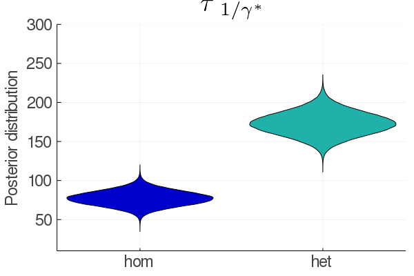
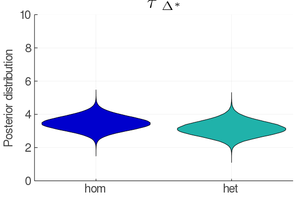
Figure 2: Comparison of the posterior distributions of the population hyper-parameters (HP) $\bm{\tau}$ for heterozygous (green) and homozygous (blue) clones. Left: HP related to the quiescence exit ($1/\tau^{*}$). Lower values indicate a higher rate of exit of quiescence. Middle: HP related to the initial (i.e., without treatment) propensity of mutated HSCs to invade the stem cell pool ($\Delta(0)$). Higher values indicate a higher propensity to invade the stem cell pool, that is, more self-renewal divisions than differentiated ones. Right: HP related to the effect of the dose in dose-response relationship (5) ($\Delta^{*}$). Higher values indicate a stronger depletion of the stem cell pool.

3.2 Individual responses to the therapy

In the selected model $\mathcal{M}$, variations of IFN$\alpha$ impact $\bar{\Delta}_{het}^{*}$ and $\bar{\Delta}^{*}_{hom}$ through the affine sigmoid relationship (5) which involves two parameters: the initial value $\Delta$ (without IFN$\alpha$, that we also writte for clarity: $\Delta(0)$) and $\Delta^{*}$ that can be interpreted as a slope for the dose-response relationship. The posterior distributions of these parameters, both for heterozygous and homozygous malignant subclones, have been estimated for each patient, as well as a population effect through our hierarchical Bayesian inference framework. Those distributions are displayed in Fig. 3. Note that not all patients in our cohort present homozygous HSCs. We observe some inter-individual heterogeneity; patients respond differently to the therapy as already evidenced by Mosca et al. [26]. The inferred population effect, described by a (truncated) Normal law (see eq. 10) with (posterior) mean $\mathds{E}[\bm{\tau}|\mathcal{D}]$ and variance $\mathds{E}[\bm{\sigma^{2}}|\mathcal{D}]$, is also displayed in Fig. 3. The estimations for the other parameters involved in model $\mathcal{M}$ are presented in Fig. E.3.

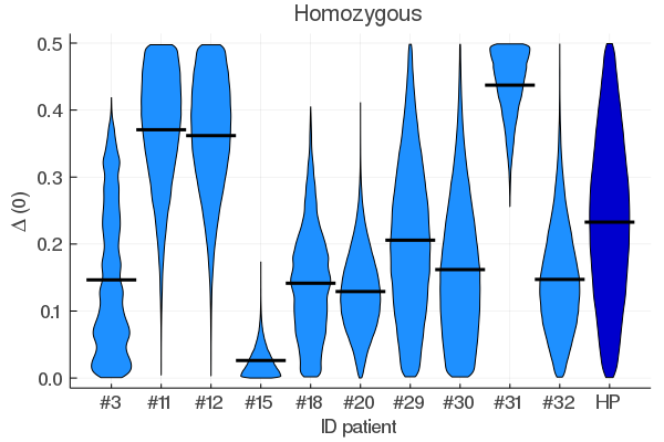
Figure 3: Posterior distributions of the parameters involved in the dose-response relationships of $\bar{\Delta}_{hom}^{*}$ (left) and $\bar{\Delta}_{het}^{*}$ (right) estimated for each patient. HP indicates the population distribution, described by a (truncated) Gaussian distribution (10) with mean $\mathds{E}[\bm{\tau}|\mathcal{D}]$ and variance $\mathds{E}[\bm{\sigma^{2}}|\mathcal{D}]$. At the top, we display the distributions for parameter $\Delta^{*}$ that can be seen as the slope in the affine sigmoid relationships (5), and at the bottom the initial propensity of the mutated cells to invade the stem cell pool ($\Delta(0)$). For parameters related to homozygous cells, only patients that exhibit homozygous clones are presented. Horizontal lines indicate mean values.

Then, for each patient, by sampling from his posterior distribution using a Monte-Carlo method, we propagate the uncertainties from the parameters to the model output and display the hematopoietic dynamics over the treatment. Figure 4 presents three examples when Fig. E.2 presents all dynamics. Compared to the previous results from Mosca et al., it is interesting to observe that some late data points (at about 2,000 days for patients #20, 25, and 32), that were previously considered as outliers, are now with our improved model the reflect of a decrease of the dosage (or even a treatment interruption) and the sign of a relapse. Such results indicate that the dosage should not be decreased in a too large extent.

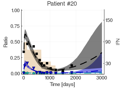
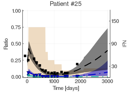
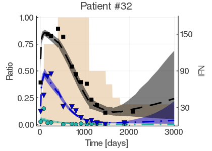
Figure 4: Examples of inferred dynamics and comparison to the data. Black lines correspond to the inferred VAF in mature cells. Blue and green lines correspond to the inferred CF in homozygous and heterozygous progenitor cells, respectively. The dots, triangles and squares are the experimental data values. The shaded areas represent 95% credibility intervals. The shaded beige areas correspond to the dose of IFN$\alpha$ received over time.

3.3 Estimating individual minimal doses

From the estimation results, we see that MPN patients differently respond to the treatment, and that, there is a risk of relapse if the dose of IFN$\alpha$ is decreased. In the selected model $\mathcal{M}$, the relapse is explained by the fact that decreasing dose $d$ also increases the propensity of mutated HSCs to invade the stem cell pool, i.e., $\bar{\Delta}^{*}$ is a decreasing function of $d$. In Fig. 5, we display for all patients the estimated dose-response relationships $\bar{\Delta}^{*}_{het}$ and $\bar{\Delta}^{*}_{hom}$ (for the latter, only if the patient has homozygous subclones) by taking, for the parameters involved in both relations, the means of the posterior distributions for $\Delta_{het}(0),\Delta_{hom}(0),\Delta_{het}^{*}$ and $\Delta^{*}_{hom}$.

Figure 5: Dose-response relationships for $\bar{\Delta}_{het}^{*}$ (green) and $\bar{\Delta}^{*}_{hom}$ (blue) as function of the weekly IFN$\alpha$ dose $d$. Each curve represents a patient. Extremities of the curves correspond to the minimum and maximum dose they received over the treatment. Points and triangles respectively refer to the value of $\bar{\Delta}_{het}^{*}$ and $\bar{\Delta}_{hom}^{*}$ at the averaged dosage received over the 450 first days of therapy by the patient.

Since $\Delta^{*}_{het}(0)>0$ and $\bar{\Delta}^{*}$ is a decreasing function of $d$, there is, for each heterozygous patient (without homozygous HSCs), a dose $d^{\prime}$ such that $\bar{\Delta}_{het}^{*}(d^{\prime})=0$ and $\bar{\Delta}^{*}_{het}(d)>0$ for $d<d^{\prime}$ (and we naturally extend the definition of $d^{\prime}$ in the case of patients having simultaneously homozygous and heterozygous HSCs). Since we obtain the (posterior) distributions of parameters, we can give the credibility intervals of the dose-response relationships to illustrate their uncertainty, as displayed for example in Fig. 6 (left) for patient #32. In particular, $d^{\prime}$ cannot be known for sure, but we can estimate for all possible doses $d$ the probability of remission $P_{rem}(d)$ (see eq. 13), which is also equal to $P_{rem}(d)=\mathds{P}[d>d^{\prime}]$. Such probability is displayed for patient #32 in Figure 6 (right side). We define the minimal IFN$\alpha$ dose for a patient $i$ by $d^{(i)}_{min}$ such that $P_{rem}(d^{(i)}_{min})=0.95$. For patient #32, this minimal dose is estimated to 72 µg/week.

Figure 6: On the left, dose-response relationships of $\bar{\Delta}^{*}_{het}$ and $\bar{\Delta}^{*}_{hom}$ for patient #32 along with 95% credibility intervals. On the right, probability of remission $P_{rem}$ as a function of the dose. Red dashed lines indicate the dose above which there is a 95% chance of getting a remission, which is $d^{(i)}_{min}=72$ µg/week for patient $i:=32$.

The minimal dose can then be computed for each patient of our cohort (Fig. 7), similarly to what was presented for patient #32 . Our results can then be used as guidelines for the clinicians: notably to discourage an abrupt dose de-escalation or a decrease of the IFN$\alpha$ dose for a given patient under the estimated lower limit, since it would increase the risk of relapse.

Figure 7: Estimation of the minimal dose that should be given to each patient. The x-axis indicates a dose de-escalation, from 135 µg/week (left) to 0 µg/week (right). Decreasing the dose also decreases the probability of remission. Vertical black lines indicate the minimal estimated IFN$\alpha$ dose $d^{(i)}_{min}$ that should be given to patient $i$ such that there is a 95% chance of getting a long-term molecular remission.

3.4 Determining an initial treatment dose

In the previous section, we computed for all patients of our observational cohort a personalized minimal IFN$\alpha$ dose, both necessary and sufficient to get a long-term remission. Besides, owing to the hierarchical Bayesian framework, the inference is not only at the individual level, but also at the population level.
For a new patient, we can now consider, as prior distributions for his model parameters, (truncated) Gaussian distributions of means and variances the estimated posterior means of the corresponding hyper-parameters. This new prior can be used a priori, before having any observation for this patient, and can help determining a suitable starting dose. By sampling from these new prior distributions, we can determine the prior behavior of $\bar{\Delta}^{*}_{het}$ and $\bar{\Delta}^{*}_{hom}$ according to the dose (Figure 8 left and right respectively).

Figure 8: Prior dose-response relationships of $\bar{\Delta}^{*}_{het}$ (left) and $\bar{\Delta}^{*}_{hom}$ (right) for new patients (based on the estimation made from our cohort). Lines indicate the median values, shaded areas indicate 95% credibility intervals. The black dashed horizontal line indicate $\Delta^{*}=0$. Below this limit, the treatment induces a long-term remission, according to our model.

Then, we can compute the probability of long-term remission, as a function of the dose, by considering a patient having only heterozygous, only homozygous, or both malignant subclones (Fig. 9). For a population of patients having both homozygous and heterozygous JAK2^V617FHSCs, we estimate that a starting dose of 45 µg/week might lead to a long-term remission in 86% of the cases. Our results suggest that the minimal initial dose such that 95% of the patients would reach a remission, should be equal to 71 µg/week.

Figure 9: For a new JAK2^V617Fpatient, probability of having a long-term remission as a function of the initial posology. We distinguish cases where the patients only have homozygous HSCs (blue), only heterozygous HSCs (green) or both (black). The vertical dashed line indicate the initial dose used in clinical trials [35, 22].

4 Discussion

To determine the minimal dose in IFN$\alpha$ therapy against MPN, we proposed a method combining mathematical modelling, model selection, and hierarchical Bayesian inference. We extended the model of Mosca et al. [26] to take into account the variations of posology along treatment. We proposed several alternative models and used a two-step model selection procedure: first, we discarded most models based on the AIC, then we applied a hierarchical Bayesian inference method to calibrate the remaining models. We selected the best performing model according to the DIC. Finally, we thoroughly analyzed the results obtained for the selected model. Data used for the calibration came from 19 JAK2^V617Fpatients. In agreement with [26], our results suggest that IFN$\alpha$ increases the quiescence exit of mutated HSCs, especially the homozygous ones, but we found no evidence suggesting that this response may be sensitive to variations of dosage along therapy. A possible explanation could be that homozygous HSCs exit quiescence at the beginning of the therapy and then no longer return to this state. The identified major mechanism of action by which the stem cell pool is depleted is HSCs differentiation. IFN$\alpha$ may increase the propensity of mutated HSCs to differentiate into progenitor cells as the dose increases. This mechanism of action would not differ according to the genotype, in agreement with results from [26], but contrary to the finding of Tong et al. [30], who showed using single-cell RNA-seq technique, that homozygous cells are quiescent while heterozygous cells undergo apoptosis in IFN$\alpha$-treated patients. When a minimal dose is reached, mutated HSCs face more differentiated than self-renewal divisions; long-term remission can be obtained. We estimated this minimal dose necessary and sufficient to ultimately deplete the malignant clones for all individuals in our cohort. Our data discourage de-escalating the dose, during therapy, below this lower limit. Our model never recommends a treatment interruption since it would result in a relapse. Indeed, we estimated that mutated HSCs have an initial propensity of invading the stem cell pool, a necessary condition for the expansion of the malignant clone and the appearance of the MPN symptoms, as described in [20, 33]. Then, in the absence of IFN$\alpha$, even a tiny fraction of mutated cells (that always remain with our deterministic model) would further expand. However, when the number of mutated HSCs becomes very small, our deterministic model is no longer suitable since stochastic effects predominate. It could be taken into account by extending the model. According to our estimations, the selective advantage of homozygous cells is higher than that of heterozygous cells, meaning that homozygous HSCs encounter on average more self-renewal divisions than heterozygous ones. This result is biologically consistent with homozygous HSCs having the mutation JAK2^V617Fon both alleles, increasing its effect.
With our hierarchical Bayesian framework, we inferred a population effect and estimated the minimal dose for all individuals of our cohort and determine the most suitable initial posology to prescribe to a new patient. We estimated that an initial dose of 45 µg/week, classically used in clinical trials [35, 22, 16], should only induce a long-term remission in 86% of the cases, and we advocate instead to start at about 70 µg/week. A dose escalation remains relevant. Even if we predict a remission with a low dose, it might only be reached in a very long time, and increasing the dose would improve the response to the therapy. Besides, clinicians rarely treat at low doses (e.g. 45 µg/week) during a long time, but rather rapidly increase the posology up to 90 or 135 µg/week, to achieve hematological responses. Of course, in clinical routine, physicians also have to consider additional constraints, such as the occurrence of side effects, mainly depression [24, 31]. The occurrence of side effects might force the clinician to decrease the posology or even temporarily interrupt the therapy. To extend this work, we aim to apply optimal control methods to study stop-and-go strategies and determine the period during which the treatment might be interrupted. Since we are dealing with long-term therapies, it might be relevant to interrupt them regularly, when a sufficiently low CF is reached (for which the risk of severe disorders is limited for the patient), and restart them when the CF increases again and before the reappearance of MPN symptoms. Such strategies would avoid treating a patient continuously over many years and might also prevent the development of malignant subclones that could acquire resistance to the treatment.
Our work could also be extended for predicting purposes. The posterior distribution of the hyper-parameters (related to the population distributions of the model parameters) could now be used as prior for new individuals. Using data assimilation techniques, we could predict the response to the therapy for new patients and refine our prognostic based on new observations. This work would also entail studying the choice of the population distributions (here independent truncated Gaussian laws) in more detail and also evaluate the relevance of introducing a dependency between our hyper-parameters.
To conclude, the proposed mathematical approach, used to determine a minimal dose to prescribe, remains general and can be applied in a wide range of problems. Our method illustrates how a model selection procedure can help decipher the mechanism of action of treatment and the potential of hierarchical Bayesian statistics, both for increasing the robustness of the estimations made on an observed cohort of individuals and generalizing results to new patients.

Author contributions

G.H., I.P., P.-H.C. conceived the mathematical model, G.H., P.-H.C. defined and performed the statistical methods, W.V. advised the study, G.H., I.P., P.-H.C. wrote the manuscript, I.P, P.-H.C. supervised the study, all authors revised the manuscript.

Conflict-of-interest disclosure

The authors declare no competing financial interests.

Appendix

The base model from Mosca et al. [26] that we extend in this work is presented in the Appendix A. We derive an analytical solution for this model in § A.1 and show its practical identifiability in Appendix C. The data used for this work are presented in B. Our inference method is detailed in § C.2. Additional results of our two-step model selection procedure are presented in Appendix D, and finally, Appendix E details the results we get for the selected model.

Appendix A Details of the base model

In the base model, as presented in brief in § 2.1.1 and detailed in Mosca et al. [26], we consider three populations of hematopoietic cells: wild-type (wt), heterozygous (het), or homozygous (hom). The cell quantities of each population follow the following ODE system (here, we do not make precise the cell genotype):

$$\left\{\begin{array}[]{ll}\frac{dN_{1}(t)}{dt}&=-\gamma N_{1}(t)+\beta N_{2}(t)\\ \frac{dN_{2}(t)}{dt}&=\gamma N_{1}(t)+(\alpha\Delta-\beta)N_{2}(t)\\ \frac{dN_{i}(t)}{dt}&=\alpha(1-\Delta)\kappa_{i}N_{2}(t)-\delta_{i}N_{i}(t)\\ \frac{dN_{m}(t)}{dt}&=\delta_{i}\kappa_{m}N_{i}(t)-\delta_{m}N_{m}(t)\\ \end{array}\right.$$

with $\alpha,\beta,\gamma,\kappa_{i},\kappa_{m},\delta_{i},\delta_{m}>0$ and $\Delta\in[-1,1]$.
As presented in the next section, we can derive an analytical solution and thus avoid solving this system numerically.

A.1 Analytical solution for the base model

A.1.1 Solution for HSC compartments

The two first equations can be written in a matrix form:

$$\frac{d\bm{N}(t)}{dt}=\bm{A}\bm{N}(t)$$ (A.1)

with $\bm{N}(t):=\left(N_{1}(t),N_{2}(t)\right)^{t}$ and:

$$\bm{A}=\begin{pmatrix}-\gamma&\beta\\ \gamma&-\beta+\alpha\Delta\end{pmatrix}$$

The characteristic polynomial of $\bm{A}$ is:

$$p_{\bm{A}}(X) =X^{2}-\text{tr}(\bm{A})X+\text{det}(\bm{A})$$

$$=X^{2}+(\gamma+\beta-\alpha\Delta)X-\gamma\alpha\Delta$$

The eigenvectors of $\bm{A}$ are the polynomial roots of $p_{\bm{A}}(X)$. Its discriminant is:

$$D=(\gamma+\beta-\alpha\Delta)^{2}+4\gamma\alpha\Delta$$ (A.2)

Potentially, we should distinguish cases according to the sign of $D$, but it is possible to show that $D>0$ (see section A.1.2). Then, the two eigenvalues are distinct real numbers:

$$\lambda_{\pm}=\frac{-(\gamma+\beta-\alpha\Delta)\pm\sqrt{D}}{2}$$

with their associated eigenvectors $\bm{P_{\pm}}$:

$$\bm{P_{\pm}}=\left(1,\frac{\lambda_{\pm}+\gamma}{\beta}\right)^{t}$$

Let $\bm{P}=\left(\bm{P_{+}}|\bm{P_{-}}\right)$ and $\bm{D}$ be the diagonal matrix, we get:

$$\bm{D}=\begin{pmatrix}\lambda_{+}&0\\ 0&\lambda_{-}\end{pmatrix}$$

$$\bm{P}=\begin{pmatrix}1&1\\ \frac{\lambda_{+}+\gamma}{\beta}&\frac{\lambda_{-}+\gamma}{\beta}\end{pmatrix}$$

$$\bm{P^{-1}}=\frac{-\beta}{\sqrt{D}}\begin{pmatrix}\frac{\lambda_{-}+\gamma}{\beta}&-1\\ -\frac{\lambda_{+}+\gamma}{\beta}&1\end{pmatrix}$$

We have $\bm{A}=\bm{P}\bm{D}\bm{P^{-1}}$. Then, system (A.1) is equivalent to:

$$\bm{N}(t) =\bm{P}e^{\bm{D}t}\bm{P^{-1}}\bm{N}(0)$$

$$=\begin{pmatrix}1&1\\ \frac{\lambda_{+}+\gamma}{\beta}&\frac{\lambda_{-}+\gamma}{\beta}\end{pmatrix}\begin{pmatrix}e^{\lambda_{+}t}&0\\ 0&e^{\lambda_{-}t}\end{pmatrix}\frac{-\beta}{\sqrt{D}}\begin{pmatrix}\frac{\lambda_{-}+\gamma}{\beta}&-1\\ -\frac{\lambda_{+}+\gamma}{\beta}&1\end{pmatrix}\bm{N}(0)$$

$$=\frac{-\beta}{\sqrt{D}}\begin{pmatrix}1&1\\ \frac{\lambda_{+}+\gamma}{\beta}&\frac{\lambda_{-}+\gamma}{\beta}\end{pmatrix}\begin{pmatrix}\frac{\lambda_{-}+\gamma}{\beta}e^{\lambda_{+}t}&-e^{\lambda_{+}t}\\ -\frac{\lambda_{+}+\gamma}{\beta}e^{\lambda_{-}t}&e^{\lambda_{-}t}\end{pmatrix}\bm{N}(0)$$

$$=\frac{-\beta}{\sqrt{D}}\begin{pmatrix}\frac{\lambda_{-}+\gamma}{\beta}e^{\lambda_{+}t}-\frac{\lambda_{+}+\gamma}{\beta}e^{\lambda_{-}t}&e^{\lambda_{-}t}-e^{\lambda_{+}t}\\ \frac{(\lambda_{-}+\gamma)(\lambda_{+}+\gamma)}{\beta^{2}}(e^{\lambda_{+}t}-e^{\lambda_{-}t})&\frac{\lambda_{-}+\gamma}{\beta}e^{\lambda_{-}t}-\frac{\lambda_{+}+\gamma}{\beta}e^{\lambda_{+}t}\end{pmatrix}\bm{N}(0)$$

Finally, the solutions of (A.1) are:

$$N_{1}(t)=-\frac{\beta}{\sqrt{D}} \left[\left(\frac{\lambda_{-}+\gamma}{\beta}N_{1}(0)-N_{2}(0)\right)e^{\lambda_{+}t}-\left(\frac{\lambda_{+}+\gamma}{\beta}N_{1}(0)-N_{2}(0)\right)e^{\lambda_{-}t}\right]$$ (A.3)

$$N_{2}(t)=-\frac{\beta}{\sqrt{D}} \left[\left(\frac{(\lambda_{-}+\gamma)(\lambda_{+}+\gamma)}{\beta^{2}}N_{1}(0)-\frac{\lambda_{+}+\gamma}{\beta}N_{2}(0)\right)e^{\lambda_{+}t}\right.$$

$$\left.-\left(\frac{(\lambda_{-}+\gamma)(\lambda_{+}+\gamma)}{\beta^{2}}N_{1}(0)-\frac{\lambda_{-}+\gamma}{\beta}N_{2}(0)\right)e^{\lambda_{-}t}\right]$$ (A.4)

A.1.2 Proof that $D>0$

Let be $\alpha,\beta$, and $\gamma>0$. Let us consider $D$ as a function of $\Delta$:

$$D\colon\mathbb{R} \to\mathbb{R}$$

$$\Delta \mapsto(\gamma+\beta-\alpha\Delta)^{2}+4\gamma\alpha\Delta$$

$D$ is continuous and even $C^{\infty}$. For $\Delta\in\mathbb{R}$, we have:

$$D =(\gamma+\beta-\alpha\Delta)^{2}+4\gamma\alpha\Delta$$

$$=(\gamma+\beta)^{2}+\alpha^{2}\Delta^{2}-2\alpha\Delta(\gamma+\beta)+4\gamma\alpha\Delta$$

$$=\alpha^{2}\Delta^{2}+2\alpha\Delta(\gamma-\beta)+(\gamma+\beta)^{2}$$

Discriminant of the previous polynomial (of $\Delta$) is:

Discriminant $$=\frac{4\alpha^{2}(\gamma-\beta)^{2}-4\alpha^{2}(\gamma+\beta)^{2}}{2\alpha^{2}}$$

$$=2\left[(\gamma-\beta)^{2}-(\gamma+\beta)^{2}\right]$$

$$=2\left[(\gamma-\beta-\gamma-\beta)(\gamma-\beta+\gamma+\beta)^{2}\right]$$

$$=2\left[-2\beta\times 2\gamma\right]$$

$$=-8\beta\gamma<0$$

The discriminant is strictly negative, meaning that $D$ does not cancel on $\mathbb{R}$. Since $D(\Delta=0)=(\gamma+\beta)^{2}>0$, $D$ is strictly positive $\forall\alpha,\beta,\gamma>0$ and $\forall\Delta\in\mathbb{R}$.

A.1.3 Solution for immature cells

We want to derive the solution $N_{i}(t)$ of the following equation:

$$\frac{dN_{i}(t)}{dt}=\alpha(1-\Delta)\kappa_{i}N_{2}(t)-\delta_{i}N_{i}(t)$$ (A.5)

$N_{2}(t)$, expressed in (A.4), is written more concisely:

$$N_{2}(t)=A_{1}e^{\lambda_{1}t}+A_{2}e^{\lambda_{2}t}$$

Equation (A.6) can be easily solved using Duhammel’s method, and we obtain:

$$N_{i}(t)=K_{i}e^{-\delta_{i}t}+\alpha(1-\Delta)\kappa_{i}\sum_{k=1}^{2}\left(A_{k}\frac{e^{\lambda_{k}t}}{\lambda_{k}+\delta_{i}}1_{(\lambda_{k}+\delta_{i}\neq 0)}+1_{(\lambda_{k}+\delta_{i}=0)}\cdot A_{k}te^{-\delta_{i}t}\right)$$ (A.6)

with $K_{i}$ found using initial conditions, that is:

$$K_{i}=N_{i}(0)-\alpha(1-\Delta)\kappa_{i}\sum_{k=1}^{2}\left(\frac{A_{k}}{\lambda_{k}+\delta_{i}}1_{(\lambda_{k}+\delta_{i}\neq 0)}\right)$$

A.1.4 Solution for mature cells

We derive the solution $N_{m}(t)$ of the following equation:

$$\frac{dN_{m}(t)}{dt}=\delta_{i}\kappa_{m}N_{i}(t)-\delta_{m}N_{m}(t)$$ (A.7)

For simplicity, we denote:

$$N_{i}(t)=B_{1}e^{\lambda_{1}t}+B_{2}e^{\lambda_{2}t}+B_{3}e^{\lambda_{3}t}+Cte^{-\delta_{i}t}$$

with at least one of the constants $B_{1},B_{2},B_{3},C$, equal to 0 (and $C=0$ with high probability). Remember that $\lambda_{+}\neq\lambda_{-}$ because $D>0$.
As for the previous case, we use Duhammel’s method, and we get:

$$N_{m}(t)= K_{m}e^{-\delta_{m}t}$$

$$+\delta_{i}\kappa_{m}\sum_{k=1}^{3}\left(B_{k}\frac{e^{\lambda_{k}t}}{\lambda_{k}+\delta_{m}}1_{(\lambda_{k}+\delta_{m}\neq 0)}+1_{(\lambda_{k}+\delta_{m}=0)}\cdot B_{k}te^{-\delta_{m}t}\right)$$ (A.8)

$$+C\delta_{i}\kappa_{m}\left(\frac{1}{\delta_{m}-\delta_{i}}\left(t-\frac{1}{\delta_{m}-\delta_{i}}\right)1_{(\delta_{m}\neq\delta_{i})}+\frac{t^{2}}{2}1_{(\delta_{m}=\delta_{i})}\right)e^{-\delta_{i}t}$$

with $K_{m}$ found thanks to the initial conditions:

$$K_{m}=N_{m}(0)-\delta_{i}\kappa_{m}\sum_{k=1}^{3}\left(\frac{B_{k}}{\lambda_{k}+\delta_{m}}1_{(\lambda_{k}+\delta_{m}\neq 0)}\right)+C\delta_{i}\kappa_{m}\frac{1}{(\delta_{m}-\delta_{i})^{2}}1_{\delta_{m}\neq\delta_{i}}$$

A.1.5 Summary of the analytical solution

For a given set of parameters, the solution of the system (1) is:

$$N_{1}(t) =-\frac{\beta}{\sqrt{D}}\left[\left(\frac{\lambda_{-}+\gamma}{\beta}N_{1}(0)-N_{2}(0)\right)e^{\lambda_{+}t}-\left(\frac{\lambda_{+}+\gamma}{\beta}N_{1}(0)-N_{2}(0)\right)e^{\lambda_{-}t}\right]$$

$$N_{2}(t) =A_{+}e^{\lambda_{+}t}+A_{-}e^{\lambda_{-}t}$$

with:

$$A_{+} =-\frac{\beta}{\sqrt{D}}\left[\left(\frac{(\lambda_{-}+\gamma)(\lambda_{+}+\gamma)}{\beta^{2}}N_{1}(0)-\frac{\lambda_{+}+\gamma}{\beta}N_{2}(0)\right)\right]$$

$$A_{-} =+\frac{\beta}{\sqrt{D}}\left[\left(\frac{(\lambda_{-}+\gamma)(\lambda_{+}+\gamma)}{\beta^{2}}N_{1}(0)-\frac{\lambda_{-}+\gamma}{\beta}N_{2}(0)\right)\right]$$

and:

$$N_{i}(t)=K_{i}e^{-\delta_{i}t}+\alpha(1-\Delta)\kappa_{i}\left(A_{+}\frac{e^{\lambda_{+}t}}{\lambda_{+}+\delta_{i}}+A_{-}\frac{e^{\lambda_{-}t}}{\lambda_{-}+\delta_{i}}\right)$$

with:

$$K_{i}=N_{i}(0)-\alpha(1-\Delta)\kappa_{i}\left(\frac{A_{+}}{\lambda_{+}+\delta_{i}}+\frac{A_{-}}{\lambda_{-}+\delta_{i}}\right)$$

and finally:

$$N_{m}(t)=K_{m}e^{-\delta_{m}t}+\delta_{i}\kappa_{m}\left[K_{i}\frac{e^{-\delta_{i}t}}{\delta_{m}-\delta_{i}}+\alpha(1-\Delta)\kappa_{i}\left(\frac{A_{+}}{\lambda_{+}+\delta_{i}}\frac{e^{\lambda_{+}t}}{\lambda_{+}+\delta_{m}}+\frac{A_{-}}{\lambda_{-}+\delta_{i}}\frac{e^{\lambda_{-}t}}{\lambda_{-}+\delta_{m}}\right)\right]$$

with:

$$K_{m}=N_{m}(0)-\delta_{i}\kappa_{m}\left[\frac{K_{i}}{\delta_{m}-\delta_{i}}+\alpha(1-\Delta)\kappa_{i}\left(\frac{A_{+}}{(\lambda_{+}+\delta_{i})(\lambda_{+}+\delta_{m})}+\frac{A_{-}}{(\lambda_{-}+\delta_{i})(\lambda_{-}+\delta_{m})}\right)\right]$$

A.2 Normalization, initial conditions, and simplification

Data from Mosca et al. [26] do not provide information about absolute values for quantities of wt, het, or hom cells separately (that are solutions of the ODE systems), but rather their relative proportions (for more details, see Appendix B). To take this into account, we consider as outputs of our model no longer the numbers of cells but the proportions of immature heterozygous cells (and similarly for hom cells):

$$z_{het}(t)=\frac{N_{i,het}(t)}{N_{i}(t)+N_{i,het}(t)+N_{i,hom}(t)}$$

as well as the mature variant allele frequency (VAF) among granulocytes:

$$y(t)=\frac{0.5\cdot N_{m,het}(t)+N_{m,hom}(t)}{N_{m}(t)+N_{m,het}(t)+N_{m,hom}(t)}$$

Following the idea of Michor et al. [25], it is considered that IFN$\alpha$ acts by modifying the values of some parameters in the model. Time $t=0$ corresponds to the beginning of the treatment. Before that time, equations (1) are still valid, but homeostatic conditions are assumed to be satisfied, i.e., the system is in a quasi-stationary state. Homeostatic conditions are, of course, verified for wt cells as soon as $\Delta=0$, leading to the following initial conditions:

$$N_{1}(0) =\frac{\beta}{\beta+\gamma}N_{HSC}$$

$$N_{2}(0) =\frac{\gamma}{\beta+\gamma}N_{HSC}$$

$$N_{i}(0) =\frac{\kappa_{i}\alpha}{\delta_{i}}N_{2}(0)$$

$$N_{m}(0) =\frac{\kappa_{m}\delta_{i}}{\delta_{m}}N_{i}(0)$$

where $N_{HSC}$, the total wild-type HSC number, is considered constant. For mutated cells, the base model assumes that $\Delta_{het}\approx\Delta_{hom}\approx 0^{+}$. We also introduce $\eta_{het}=\frac{N_{1,het}(0)+N_{2,het}(0)}{N_{HSC}}$ and $\chi_{het}=\frac{N_{2,het}(0)}{N_{1,het}(0)+N_{2,het}(0)}$ for expressing the initial conditions for het and hom cells. From $t=0$, patients are under treatment. IFN$\alpha$ is assumed to modify the values of some parameters, potentially in different ways depending on the cell type. In terms of notation, the superscript ^∗ is added to parameters impacted by the drug. From $t\geq 0$, eq. (1) remains valid with new parameters, and there is an equilibrium shift that induces new dynamics.

Given the solutions of the ODE systems and the way we normalize them to obtain ratios, we get some simplifications. Parameter $N_{HSC}$ is not relevant anymore: no matter its value, it will not change the final output of the model (when considering the ratios $z_{het},z_{hom}$, and $y$). By introducing $k_{i,het}$ and $k_{i,hom}$ such that $k_{i,het}=\kappa_{i,het}/\kappa_{i}$ and $k_{i,hom}=\kappa_{i,hom}/\kappa_{i}$, parameter $\kappa_{i}$ has no longer been estimated. The same goes for $\kappa_{m}$.

Based on prior biological knowledge, many other assumptions are detailed and justified by Mosca et al. [26] to decrease the number of parameters to estimate for each patient. These assumptions are summarized in table A.1. For each patient, we end up with 7 parameters to estimate for the base model. To verify if these assumptions are sufficient to ensure the identifiability of the model, and before further extending the model with potentially more parameters to estimate, we generated virtual data (§ C.1) and tried to retrieve the model parameters that generated them (§ C.3).

Figure A.1: Summary table of the parameters used in the base model (from Mosca et al. [26]). NR means: Not Relevant, i.e., after normalization, these quantities simplify and no longer intervene in the model output.

Appendix B Data and observation model

Data $\mathcal{D}=\{\mathcal{D}_{i}\}_{i\in\{1,\cdots,N\}}$ come from Mosca et al. [26]. From the cohort of patients of Mosca et al., we consider $N=19$ MPN patients: those for which there are enough observations, and only those having the mutation JAK2^V617F. Identical patient IDs than in [26] are used (when displaying the results). For a patient $i$, the data consist of observations at different times $t_{k}$, from the beginning of the therapy ($t=0$), where Variant Allele Frequencies (VAF) $\hat{y}_{k}^{(i)}$ among mature cells and the clonal architecture among progenitor cells $(\hat{n}_{k}^{(i)},\hat{n}_{k,het}^{(i)},\hat{n}_{k,hom}^{(i)})$ were measured. In the following, we will omit the patient index $i$ for clarity.
We use the same observation model as Mosca et al. [26]. For mature cells, it is assumed a Gaussian noise with a variance that depends on the true VAF $y_{k}\in[0,1]$ at time $t_{k}$:

$$\hat{y}_{k}\mid y_{k}\sim\mathcal{N}\left(y_{k},y_{k}\left(1-y_{k}\right)\sigma_{m}^{2}\right)$$

with $\sigma_{m}$ to be estimated.
Concerning the observations among immature cells, we observe some counts of wt, het and hom progenitor cells at time $t_{k}$, respectively denoted by $\hat{n}_{k}$, $\hat{n}_{k,het}$ and $\hat{n}_{k,hom}$. These cells are assumed to be randomly sampled from an unknown but very large set of immature cells, so that the uncertainty might be modeled by a multinomial distribution, as it was also done in [8]:

$$\mathbb{P}\left[\hat{n}_{k}=n_{1},\hat{n}_{k,het}=n_{2},\hat{n}_{k,hom}=n_{3}\mid z_{k,het},z_{k,hom}\right]=\frac{\left(n_{1}+n_{2}+n_{3}\right)!}{n_{1}!n_{2}!n_{3}!}z_{k}^{n_{1}}z_{k,het}^{n_{2}}z_{k,hom}^{n_{\mathrm{3}}}$$

where $z_{k}$, $z_{k,het}$, and $z_{k,hom}$ are the true CF for wt, het and hom progenitor cells respectively (with $z_{k}=1-z_{k,het}-z_{k,hom}$).

Appendix C Practical Identifiability

C.1 Generating virtual data

To verify the identifiability of the base model, we generate 30 virtual patients. We sample 30 parameter vectors (from a population distribution that we choose), leading to 30 different dynamics. For each of them, we sample observation times and add some noise to reproduce the data from the cohort of Mosca et al. [26].
We only consider 19 patients in this work, yet the number of JAK2^V617Fpatients in the original cohort was higher, but many patients had only a few data points. We also consider such patients with little information in the virtual data generated here (see fig. C.2).

Five parameters values and two initial conditions are required to generate one patient’s virtual dynamics (see tab. A.1). The population distributions used to generate the parameters are the following:

• $\eta_{het}\sim\mathcal{U}([0,1])$ (uniform)

• $\eta_{hom}\sim\mathcal{U}([0,2.5])$ (uniform)

• $\Delta^{*}_{het}\sim\mathcal{N}(-0.1,0.1^{2})$ (truncated over $[-1,1]$)

• $\Delta_{hom}^{*}\sim\mathcal{N}(-0.3,0.1^{2})$ (truncated over $[-1,1]$)

• $\gamma_{het}^{*}\sim\mathcal{N}(1/40,0.01^{2})$ (truncated over $[1/300,1/10]$)

• $\gamma_{hom}^{*}\sim\mathcal{N}(1/120,0.01^{2})$ (truncated over $[1/300,1/10]$)

• $k_{m,het}\sim\mathcal{N}(10,1)$ (truncated over $[1,20]$)
  

In figure C.1, we show all parameters that have been sampled and the corresponding population distributions.

Figure C.1: Generated parameters for 30 virtual patients. Points are sampled parameters. The line represents the actual population density, from which we have sampled values.

Now that we have the true dynamics for 30 virtual patients (since our model is deterministic), we want to generate noisy data for each of them. Not all patients will have the same amount of data $n_{i}$. Indeed, to be consistent with the dataset from Mosca et al. [26], we generate a sparse data set, as depicted in figure C.2. This figure shows the distribution of the number of observation times for the virtual cohort. The mean number of observations is equal to 10 (the same as in the cohort of Mosca et al.), with some virtual patients with only 3 data points while others have 15 data points.

Figure C.2: Distribution of the number of data points $n$ sampled among our 30 virtual patients, from 3 to 15 observation times, with a mean value of 10, consistent with the cohort from Mosca et al. [26].

Then, we can generate a number $n_{i}$ of noisy observations from each virtual patient’s actual dynamics $i$. First, we generate the times (in days) when observations are made. We always consider that the first measure is made at the initial time. Then, we generate the others randomly according to the following method:

function sample_time(n)
    t = zeros(n)
    t[1] = 0.0
    for i in 2:n
        t[i] = t[i-1] + rand(truncated(Normal(100, 10),30, 300))
    end
    return t
end

to consider observations about each trimester.
Then, from the actual ratios for immature and mature cells at this time, we add some noise. We use the same noise model as described in Appendix B.

At this stage, we have 30 dataset comparable to the ones from the cohort of Mosca et al.
The objective is thus to retrieve the actual patient’s dynamics using our inference method.

C.2 Model calibration

C.2.1 Posterior distribution

The model identification method used to retrieve the parameters of all patients and the population parameters (called hyper-parameters) is the same as the one used by Mosca et al. [26].
$\bm{\theta}=\left\{\bm{\theta}^{(i)}\right\}_{i\in\{1,\cdots,N\}}$ denotes the set of all patient-related model parameters with:

$$\begin{array}[]{c}\bm{\theta}^{(1)}=\left(\theta_{1}^{(1)},\cdots,\theta_{P}^{(1)}\right)\\ \vdots\\ \bm{\theta}^{(N)}=\left(\theta_{1}^{(N)},\cdots,\theta_{P}^{(N)}\right)\end{array}$$

where $P=7$ is the number of parameters to estimate. With the hierarchical inference method, instead of estimating each $\bm{\theta}^{(i)}$ independently, we introduce some hyper-parameters (HP) $\bm{\tau}=\left(\tau_{1},\cdots,\tau_{P}\right)$ and $\bm{\sigma^{2}}=\left(\sigma_{1}^{2},\cdots,\sigma_{P}^{2}\right)$ so that, a priori:

$$\forall i\in\{1,\cdots,N\},\forall k\in\{1,\cdots,P\},\theta_{k}^{(i)}\mid\tau_{k},\sigma_{k}^{2}\sim\mathcal{N}_{c,k}\left(\tau_{k},\sigma_{k}^{2}\right)$$

where $\mathcal{N}_{c,k}$ is defined as a truncated (over a range that depends on the considered parameter $k$, as described in section C.1) Gaussian distribution. To note that, for parameters $\eta_{het}$ and $\eta_{hom}$, we do not consider hyper-parameters since there is no reason to have initial conditions sampled from population distributions. Now, we can estimate the joint posterior distributions of $\bm{\theta}^{(1)},\cdots,\bm{\theta}^{(N)}$ and hyperparameters $\bm{\tau}$ and $\bm{\sigma^{2}}$:

$$\mathds{P}\left[\bm{\theta}^{(1)},\cdots,\bm{\theta}^{(N)},\bm{\tau},\bm{\sigma^{2}}\mid\mathcal{D}\right] \propto\mathds{P}\left[\mathcal{D}\mid\bm{\theta}^{(1)},\cdots,\bm{\theta}^{(N)},\bm{\tau},\bm{\sigma^{2}}\right]\mathds{P}\left[\bm{\theta}^{(1)},\cdots,\bm{\theta}^{(N)},\bm{\tau},\bm{\sigma^{2}}\right]$$

$$\propto\mathds{P}\left[\mathcal{D}\mid\bm{\theta}^{(1)},\cdots,\bm{\theta}^{(N)}\right]\mathds{P}\left[\bm{\theta}^{(1)},\cdots,\bm{\theta}^{(N)},\bm{\tau},\bm{\sigma^{2}}\right]$$

$$\propto\prod_{i\in\{1,\cdots,N\}}\left(\mathds{P}\left[\mathcal{D}_{i}\mid\bm{\theta}^{(i)}\right]\right)\mathds{P}\left[\bm{\theta}^{(1)},\cdots,\bm{\theta}^{(N)}[\bm{\tau},\bm{\sigma^{2}}\right]\mathds{P}\left[\bm{\tau},\bm{\sigma^{2}}\right]$$

$$\propto\prod_{i\in\{1,\cdots,N\}}\left(\mathds{P}\left[\mathcal{D}_{i}\mid\bm{\theta}^{(i)}\right]\mathds{P}\left[\bm{\theta}^{(i)}\mid\bm{\tau},\bm{\sigma^{2}}\right]\right)\mathds{P}[\bm{\tau}]\mathds{P}\left[\bm{\sigma^{2}}\right]$$ (C.1)

The previous relation is obtained by considering independence between patients, conditionally on the hyper-parameter values. In addition, we further simplify the relation above by assuming that the components of our parameter and hyper-parameter vectors are independent. We get for patient $i$:

$$\mathds{P}\left[\bm{\theta}^{(i)}\mid\tau,\sigma^{2}\right]=\prod_{k\in\{1,\cdots,P\}}\mathds{P}\left[\theta_{k}^{(i)}\mid\tau_{k},\sigma_{k}^{2}\right]$$

and:

$$\mathds{P}[\bm{\tau}]=\prod_{k\in\{1,\cdots,P\}}\mathds{P}\left[\tau_{k}\right]$$

$$\mathds{P}\left[\bm{\sigma^{2}}\right]=\prod_{k\in\{1,\cdots,P\}}\mathds{P}\left[\sigma_{k}^{2}\right]$$

Likelihood $\mathds{P}\left[\mathcal{D}_{i}\mid\bm{\theta}^{(i)}\right]$ is expressed according to the observation model described in Appendix B.

C.2.2 Conditional laws of the hyper-parameters

The resulting posterior distribution is approximated numerically using the Metropolis-Hasting within Gibbs algorithm. Before using this computational method, it is useful to express the HP conditional posterior distributions.
Concerning hyper-parameter $\bm{\tau}$, for $k\in\{1,\cdots,P\}$, by keeping in (C.2.1) only the terms involving $\tau_{i}$ (since we are here only interested in its distribution ignoring a multiplication factor), we get:

$$\mathds{P}\left[\tau_{k}|\bm{\theta^{(1)}},\cdots,\bm{\theta^{(N)}},\bm{\sigma^{2}},\mathcal{D}\right]\propto\mathds{P}\left[\theta_{k}^{(1)}|\tau_{k},\sigma_{k}^{2}\right]\cdots\mathds{P}\left[\theta_{k}^{(N)}|\tau_{k},\sigma_{k}^{2}\right]\mathds{P}\left[\tau_{k}\right]$$

Prior distributions for $\tau_{k}$ are chosen uniform over intervals $[a_{k},b_{k}]$ with the same upper and lower bounds that the ones used to truncate the Gaussian law for $\theta_{k}|\tau_{k},\sigma^{2}_{k}$. Thus, we derive the (conditional posterior) probability density function $f_{\tau_{k}}$ for $t\in\mathds{R}$:

$$f_{\tau_{k}}(t) \propto\frac{1}{\sqrt{2\pi\sigma^{2}_{k}}}\exp\left(-\frac{1}{2\sigma_{k}^{2}}(\theta_{k}^{(1)}-t)^{2}\right)\cdots\frac{1}{\sqrt{2\pi\sigma^{2}_{k}}}\exp\left(-\frac{1}{2\sigma_{k}^{2}}(\theta_{k}^{(N)}-t)^{2}\right)1_{[a_{k},b_{k}]}(t)$$

$$\propto\exp\left(-\frac{1}{2\sigma_{k}^{2}}\left((\theta_{k}^{(1)}-t)^{2}+\cdots+(\theta_{k}^{(N)}-t)^{2}\right)\right)1_{[a_{k},b_{k}]}(t)$$

Since we have:

$$(\theta_{k}^{(1)}-t)^{2}+\cdots+(\theta_{k}^{(N)}-t)^{2} =\sum_{i\in\{1,\cdots,N\}}(\theta_{k}^{(i)})^{2}+Nt^{2}-2t\sum_{i\in\{1,\cdots,N\}}\theta_{k}^{(i)}$$

$$=N(t-\frac{1}{N}\sum_{i\in\{1,\cdots,N\}}\theta_{k}^{(i)})^{2}+\cdots$$

where symbol $\cdots$ indicate terms that do not involve $t$, we finally get that:

$$f_{\tau_{k}}(t)\propto\exp\left(-\frac{N}{2\sigma_{k}^{2}}\left(t-\frac{1}{N}\sum_{i\in\{1,\cdots,N\}}\theta_{k}^{(i)}\right)^{2}\right)1_{[a_{k},b_{k}]}(t)$$ (C.2)

Thus, we deduce that $\tau_{k}$ (more precisely, its conditional posterior distribution) follows a Gaussian law that is truncated over interval $[a_{k},b_{k}]$:

$$\tau_{k}\sim\mathcal{N}_{c}(\frac{1}{N}\sum_{i\in\{1,\cdots,N\}}\theta_{k}^{(i)},\frac{\sigma_{k}^{2}}{N})$$ (C.3)

Concerning hyper-parameter $\sigma^{2}_{k}$ (for $k\in\{1,\cdots,P\}$), we do the same as for hyper-parameter $\tau_{k}$ to express $\sigma^{2}_{k}|\bm{\theta^{(1)}},\cdots,\bm{\theta^{(N)}},\bm{\tau},\mathcal{D}$ and find for its probability density function, for $t\in\mathds{R}$:

$$f_{\sigma_{k}^{2}}(t)\propto\left(\frac{1}{t}\right)^{N/2+1}\exp\left(-\frac{1}{2t}\sum_{i\in\{1,\cdots,N\}}\left(\theta_{k}^{(i)}-\tau_{k}\right)^{2}\right)1_{[a^{\prime}_{k},b^{\prime}_{k}]}(t)$$

where we considered that $\sigma^{2}_{k}$ followed an improper prior distribution - namely an inverse-gamma (0,0) law - truncated over $[a^{\prime}_{k},b^{\prime}_{k}]$ (we choose $a^{\prime}_{k}=0$ and $b^{\prime}_{k}=2$). We recognise the expression of a (truncated) inverse-gamma law. As a reminder, a random variable $X$ that follows an inverse-gamma law of parameters $\alpha,\beta$ has for its density, for $x\in\mathds{R}$:

$$f_{X}(x)=\frac{\beta^{\alpha}}{\Gamma(\alpha)}(1/x)^{\alpha+1}\exp(-\beta/x)$$

Then, $\sigma^{2}_{k}|\bm{\theta^{(1)}},\cdots,\bm{\theta^{(N)}},\bm{\tau},\mathcal{D}$ follows a (truncated) inverse-gamma law with parameters $\alpha_{k}=\alpha=P/2$ and $\beta_{k}=1/2\sum_{i\in\{1,\cdots,N\}}\left(\theta_{k}^{(i)}-\tau_{k}\right)^{2}$.

C.2.3 Metropolis within Gibbs algorithm

The previous joint posterior distribution (C.2.1) is estimated by generating a Markov-Chain Monte-Carlo (MCMC). We use the Metropolis within Gibbs algorithm, which allows to iteratively sample values for parameters $\bm{\theta}^{(1)},\cdots,\bm{\theta}^{(N)}$ and hyper-parameters $\bm{\tau}$ and $\bm{\sigma^{2}}$. After initializing the MCMC chain, we successively sample HP values and then parameter values for each patient (independently, conditionally on the HP values).

To initialize the parameter values for each patient, we first run an optimization algorithm - namely the CMA-ES algorithm - to find the parameter vector that maximizes the likelihood. The CMA-ES algorithm also provides a covariance matrix that we will use for the proposal in the Metropolis-Hasting scheme. HP are initialized randomly.

We use the Gibbs method for sampling values for hyper-parameters (component-wise). The proposal of the Metropolis algorithm is the conditional posterior law (that we made explicit in the previous section). With this choice, the new sample is always accepted.

Then, conditionally on the HP values previously sampled, we sample parameters values for each patient, one by one. This is achieved using a standard Metropolis-Hasting scheme, with a Multivariate Gaussian law for the proposal. As a setting of the algorithm, a proper choice for the covariance matrix has to be found. We choose to set the proposal’s covariance matrix the one estimated by the CMA-ES algorithm (adjusted by a multiplication factor tuned to get suitable acceptance rates).
The algorithm pursues a huge number of iterations until achieving convergence (when the ergodic means do not vary anymore).

Model calibration was achieved by implementing the previous methods in Julia programming language.
The codes used for this work are available. The framework used for parameter estimation (and that can be used for a wide range of problems) is available at:

https://gitlab-research.centralesupelec.fr/2012hermangeg/bayesian-inference

The implementation of the base model and the settings to use the previous inference framework is available at:

https://gitlab-research.centralesupelec.fr/2012hermangeg/identifiability-base-model

C.3 Results of the identifiability

We ran the previous estimation method over 13 million iterations, with a burn-in length of 2 million.
All the predicted dynamics are presented in figure C.4 for our 30 patients. We also compare the predicted dynamics (solid lines) with the actual dynamics (dash lines). There is good agreement between both.
Figure C.3 compares predicted vs. actual HSC Clonal Fractions (CF) for heterozygous and homozygous cells. Values are taken at the same times like the ones in our dataset. Even if we do not have data for HSCs, the estimation method can find the true values with accuracy.

Figure C.3: Comparison of the true HSC clonal fractions and the inferred ones. The values are taken at the observations time from our virtual data set. Blue triangles refer to homozygous HSCs, green circles to heterozygous HSCs.

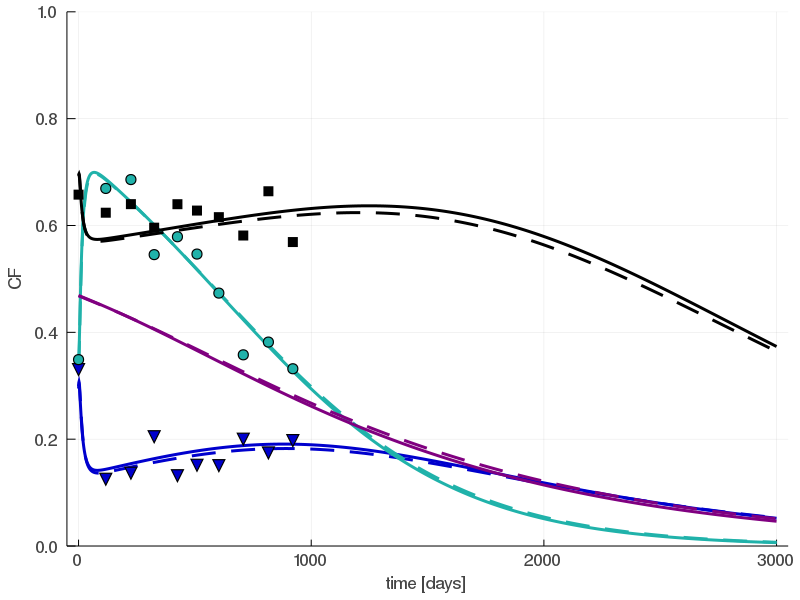
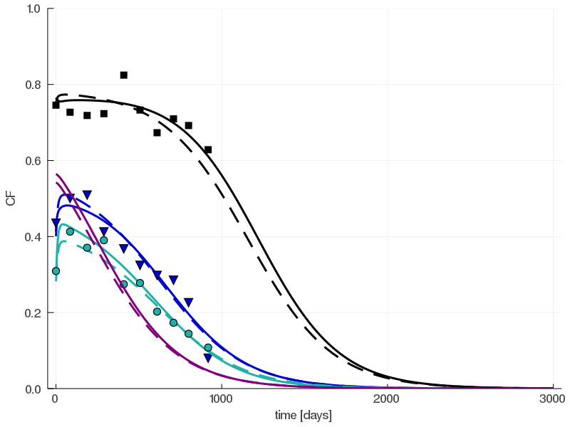
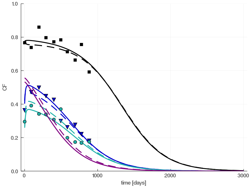
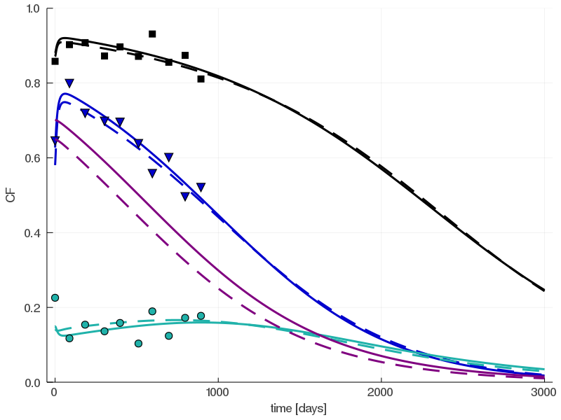
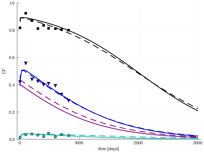
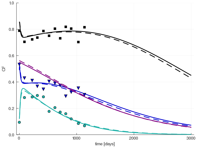
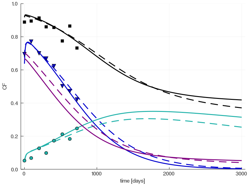
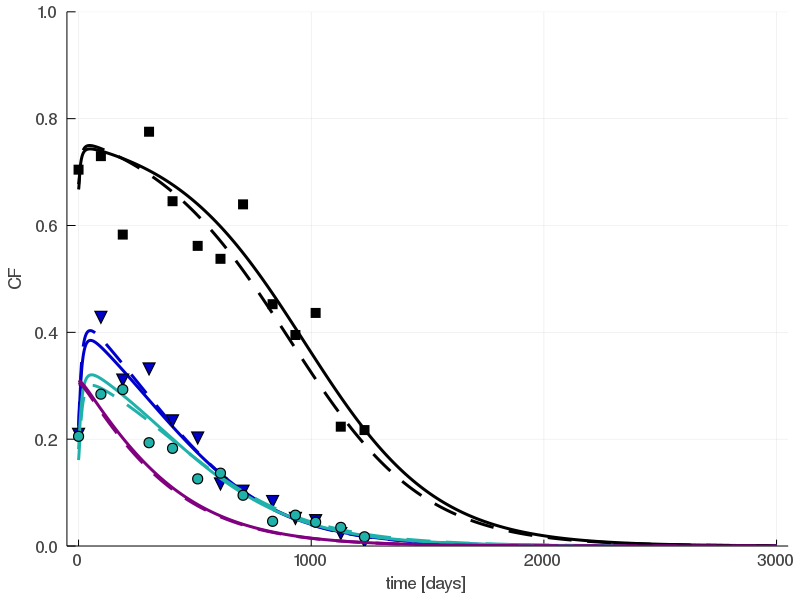
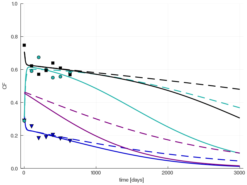
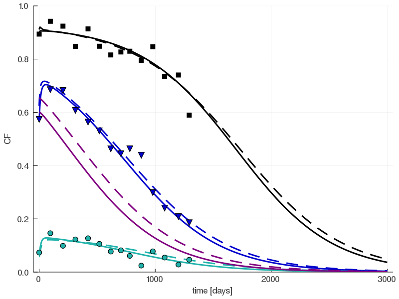
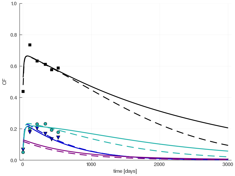
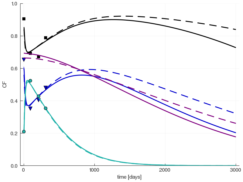
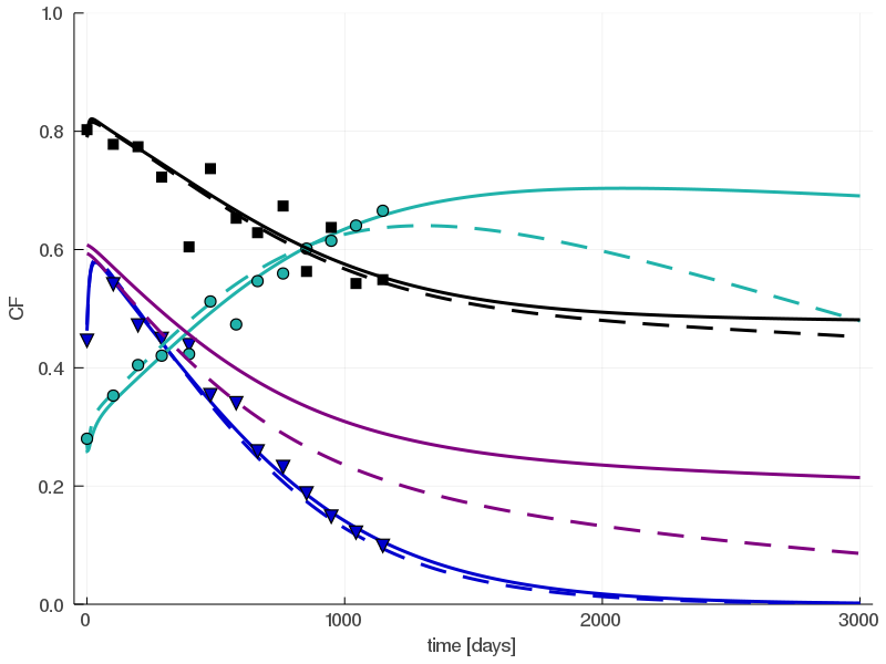
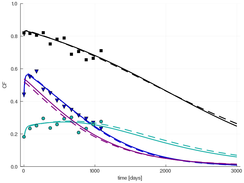
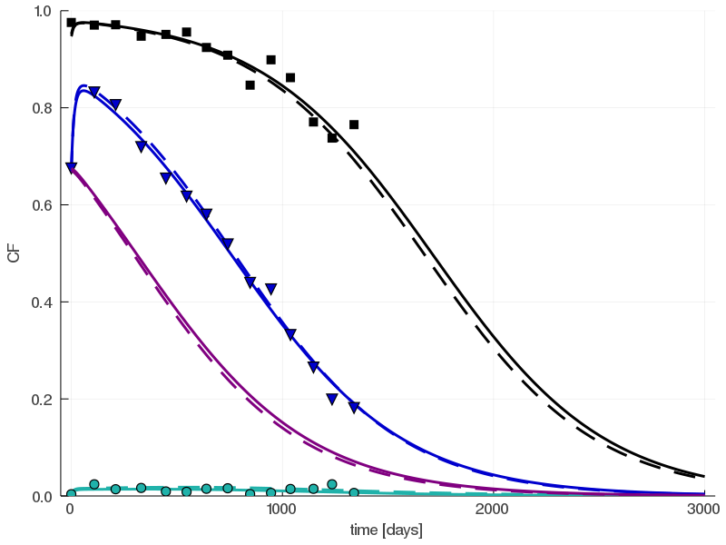
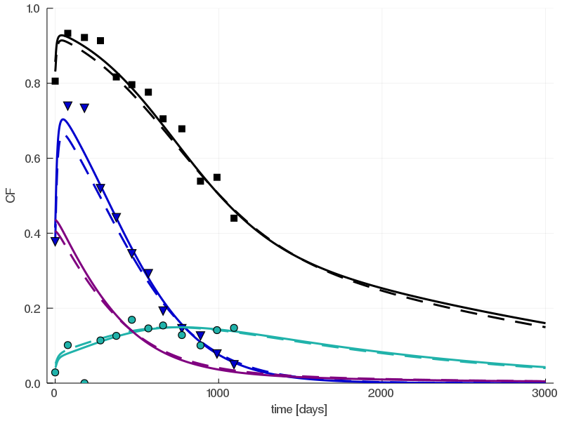
Figure C.4: Comparison of true and estimated dynamics for our 30 virtual patients. Dash lines are the true dynamics. Solid lines are the estimated dynamics (based on the median estimated parameter vector). The black squares, green circles and blue triangles are our noisy data for mature VAF, immature heterozygous and homozygous clonal fractions respectively. The purple line refers to the HSC mutated VAF.

At the individual level, the parameter estimation results are shown in fig. C.5. $\eta_{het}$, $\eta_{hom}$, $\gamma^{*}_{het}$, $\gamma^{*}_{hom}$ and $\Delta^{*}_{het}$ are quite good inferred, with 95% credibility intervals that always contain the true value. $k_{m}$ is poorly estimated: all values concentrate around 10.5 so that the population’s effect seems to predominate over inter-individual variability, suggesting that the model output might not be so highly sensitive to the value $k_{m}$. Unlike $\Delta^{*}_{het}$, $\Delta^{*}_{hom}$ is not predicted with accuracy, and we see a substantial population’s effect, thas was not seen for heterozygous HSCs. This might be because true values for $\Delta^{*}_{hom}$ are lower than those for $\Delta^{*}_{het}$. Low values might induce a stiffer increase within the first days of therapy, so that it is more tedious to estimate the value with accuracy since we do not have data for the very first days of therapy (except at the initial time).

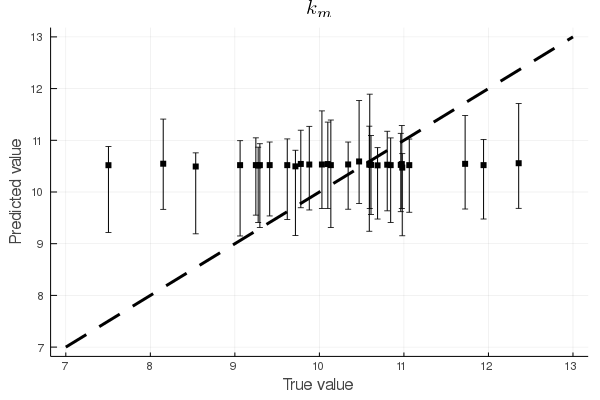
Figure C.5: Comparison between true and inferred parameters values for our 30 virtual patients. Inferred values are presented with their 95% credibility intervals.

We now analyze the previous results at a population level: we compare the estimated population’s density to the actual one. Results are shown in figure C.6. In orange, we have the results of the estimation. We see from this figure how we can infer not only the individual values but also the population’s density. It works very well for $\gamma^{*}_{het}$. For $\Delta^{*}_{hom}$ we also have good results, even if we predict less variance than in reality, but the mean of the population’s density is very well estimated. This is interesting because the estimations at the individual level were not so good. For $k_{m}$, the mean of the population’s density is quite well estimated, but the variance is lower than in reality.

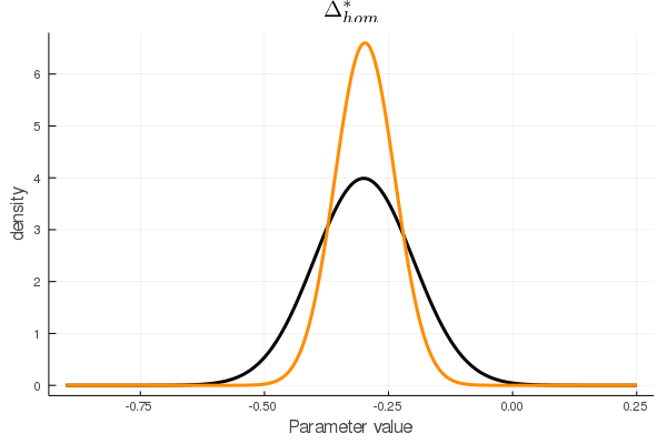
Figure C.6: Comparison of the true population’s density (black) used to generate the parameters values and the ones estimated (orange) through our hierarchical Bayesian framework. Density in orange is the estimated population’s density. That is, a truncated Gaussian law with mean and variance that are estimated hyper-parameters (mean value of their posterior distributions).

Finally, this practical identifiability study demonstrates the ability of our estimation method to infer with accuracy the patient’s dynamics. We also see that most of the parameters are well estimated at the individual level and that the hierarchical framework can retrieve the population distributions that generate the individual parameters.

Appendix D Detailed results of the model selection procedure

The first step in our model selection procedure is to calibrate all 225 models for 19 MPN patients. This results in a vast amount of models to calibrate, and there is thus a need for an efficient inference method. For this purpose, we use the CMA-ES algorithm to compute the maximum of likelihood $\mathcal{L}_{i,j}$ for each model $\mathcal{M}_{j}$, given data from patient $i$.
For all models, the likelihood is expressed using the same observation model as described in Appendix B.
Then, we compute the AIC (see eq. 8) for each combination: patient $\times$ model. Results are displayed in Fig. D.1 (and Fig. 1 to compare the models that perform the best). Each dot corresponds to a model; the horizontal line corresponds to the AIC obtained with the base model. This latter was already a good model, with very good fits for patients #6, 15, 16, 19. However, the base model had the inconvenience of resulting in very poor fits for other patients, such as patients #20, 23, 31. Thus, there was a need for a model performing better for all patients of the cohort.

Figure D.1: AIC_i,j for each model $j$ and each patient $i$.

Figure D.2: Global AIC_j for each model $j$. The orange horizontal line represents the global AIC of the base model.

Nevertheless, the best model for a given patient is not necessarily the best for another one. To compare the models, not at the individual level but the population (of our 19 JAK2^V617Fpatients) level, we compute a global AIC (see eq. 9) that sums the contribution of all individual AIC. In Fig. D.2, we display the global AIC of all models and compare them to the global AIC of the base model (horizontal orange line). Many models improve the base model on the whole cohort. In particular, three models stand out, with a global AIC of around 2,000. They are presented in Tab. 1, and we display how they perform for each patient in Fig. D.3. These models are the following:

• Model ”orange”: a constant dose-response relationship for $\bar{\gamma}^{*}_{het}$ and $\bar{\gamma}^{*}_{hom}$, a sigmoid affine one for $\bar{\Delta}^{*}_{hom}$, and an affine one for $\bar{\Delta}^{*}_{het}$

• Model ”red”: constant dose-response relationship for $\bar{\gamma}^{*}_{het}$, a linear one for $\bar{\gamma}^{*}_{hom}$, a sigmoid affine one for $\bar{\Delta}^{*}_{hom}$, and an affine one for $\bar{\Delta}^{*}_{het}$

• Model ”blue”: constant dose-response relationships for $\bar{\gamma}^{*}_{het}$ and $\bar{\gamma}^{*}_{hom}$, and a sigmoid affine one for $\bar{\Delta}^{*}_{hom}$ and $\bar{\Delta}^{*}_{het}$

Models ”orange” and ”red” are better than the base model for 11 (over 19) patients, and model ”blue” improve the fits of 12 patients.

To note that, instead of the AIC, we could have used the Bayesian Information Criterion (BIC), defined by:

$$BIC_{i,j}=-2\log\left(\mathcal{L}_{i,j}\right)+k_{j}\cdot\log\left(N_{i}\right)$$

with $N_{i}$ the number of data points (both for mature and progenitor cells) for patient $i$. The same three best models were selected when applying this criterion.

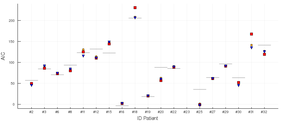
Figure D.3: Focus on the 3 best model according to their global AIC. The orange circle corresponds to the model with a constant dose-response relationships for $\bar{\gamma}^{*}_{het}$ and $\bar{\gamma}^{*}_{hom}$, a sigmoid affine one for $\bar{\Delta}^{*}_{hom}$, and an affine one for $\bar{\Delta}^{*}_{het}$. The red square corresponds to the model with a constant dose-response relationship for $\bar{\gamma}^{*}_{het}$, a linear one for $\bar{\gamma}^{*}_{hom}$, a sigmoid affine one for $\bar{\Delta}^{*}_{hom}$, and an affine one for $\bar{\Delta}^{*}_{het}$. The blue triangle corresponds to the model with a constant dose-response relationships for $\bar{\gamma}^{*}_{het}$ and $\bar{\gamma}^{*}_{hom}$, and a sigmoid affine one for $\bar{\Delta}^{*}_{hom}$ and $\bar{\Delta}^{*}_{het}$. Horizontal black line corresponds to the base model. y-axis is truncated for clarity.

In a second step, we only consider the three models that stand out and further compare them using a more rigorous hierarchical Bayesian inference method.
The same estimation method used for our virtual dataset (Appendix C) is used. Results are presented in Tab. 1. The selected model is model ”blue”, with constant dose-response relationships for $\bar{\gamma}^{*}_{het}$ and $\bar{\gamma}^{*}_{hom}$ and a sigmoid affine one for $\bar{\Delta}^{*}_{hom}$ and $\bar{\Delta}^{*}_{het}$. It is interesting to see how the results are consistent across the several selection criteria. The selected model is the model that has the best AIC, DIC, and that also improves the results for 12 patients instead of 11 for the two others.

Appendix E Detailed analysis of the selected model

The best model, selected after our two-steps model selection procedure, is the one with a constant dose-response relationship for $\bar{\gamma}^{*}_{het}$ and $\bar{\gamma}^{*}_{hom}$, and a sigmoid affine relation for $\bar{\Delta}^{*}_{hom}$ and $\bar{\Delta}^{*}_{het}$.
To visualize to which extent this model fits well the cohort data, we compare in Fig. E.1 the observed and inferred values, both for mature cells (VAF) and for het and hom progenitor cells (CF). We observe overall a good agreement between observations and inferred values.

Figure E.1: Comparison between the observed ratios (CF for progenitor cells, VAF for mature cells) and the estimated ones (based on the mean posterior parameter vector). With our 19 patients, we have 232 data points for mature cells and 255 for heterozygous and homozygous progenitors. The linear dotted line represents exact fit.

Fig. E.2 displays the inferred dynamics with 95% credibility intervals for the mature VAF and progenitor CF. There is a good agreement between observed and inferred values for most patients. We also display on this figure how the IFN$\alpha$ doses vary over therapy for each patient. It is interesting to observe how the proportion of mutated cells increases when the dose decreases to a too large extent. This model outperforms the base model of Mosca et al. [26], particularly for patients #23, 31, 20, and 25.

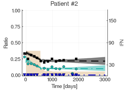
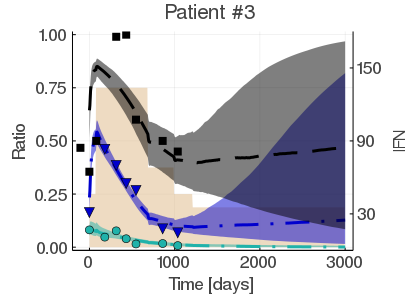
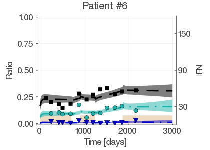
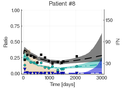
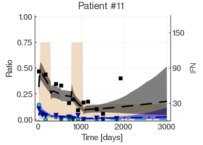
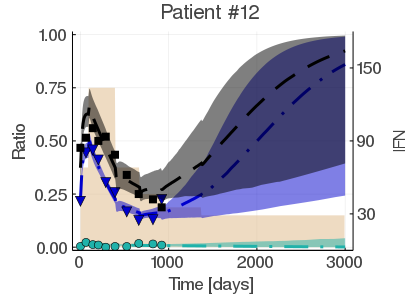
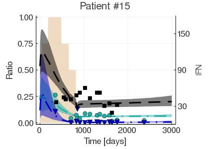
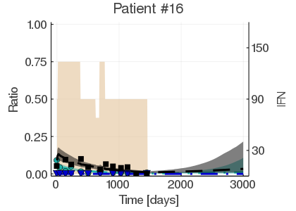
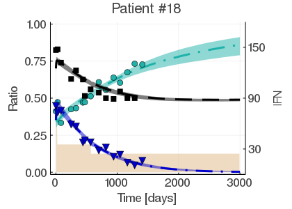
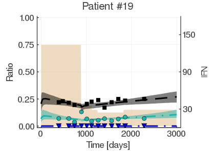
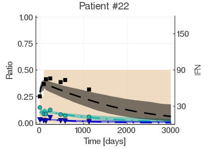
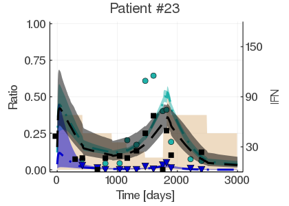
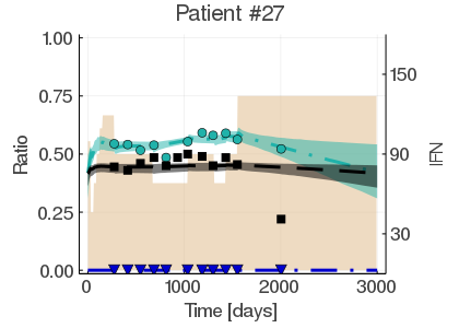
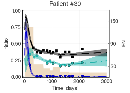
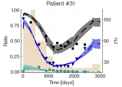
Figure E.2: Dynamics of inferred homozygous and heterozygous mutated progenitors (CF), and mature cells (VAF) are presented for 19 JAK2^V617Fpatients for whom we made the parameter estimation using our hierarchical Bayesian framework and the selected model. Triangles, dots, and squares are experimental data values. The curves were determined with the model (median values). The shaded areas represent 95% credibility intervals. The shaded beige areas correspond to the dose of IFN$\alpha$ received overtime.

We also display in Fig. E.3 the posterior distributions of the model parameters (in complement to those presented in Fig. 3).

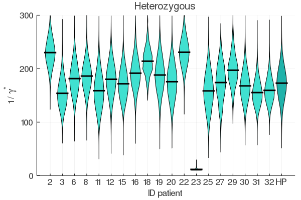
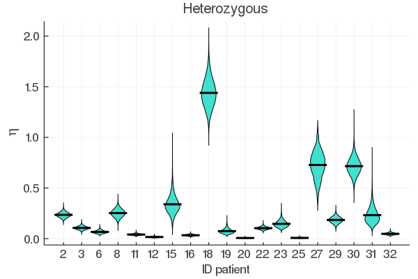
Figure E.3: Posterior distributions of the parameters. HP indicates the population distribution, described by a (truncated) Gaussian distribution (10) with mean $\mathds{E}[\bm{\tau}|\mathcal{D}]$ and variance $\mathds{E}[\bm{\sigma^{2}}|\mathcal{D}]$. For parameters related to homozygous cells (blue), only patients that exhibit homozygous clones are presented. Horizontal lines indicate mean values.

References

- [1] Akaike, H. A new look at the statistical model identification. IEEE transactions on automatic control 19, 6 (1974), 716–723.
- [2] Andrieu, C., and Thoms, J. A tutorial on adaptive mcmc. Statistics and computing 18, 4 (2008), 343–373.
- [3] Barbui, T., Vannucchi, A. M., De Stefano, V., Masciulli, A., Carobbio, A., Ferrari, A., Ghirardi, A., Rossi, E., Ciceri, F., Bonifacio, M., et al. Ropeginterferon alfa-2b versus phlebotomy in low-risk patients with polycythaemia vera (low-pv study): a multicentre, randomised phase 2 trial. The Lancet Haematology 8, 3 (2021), e175–e184.
- [4] Boullu, L., Pujo-Menjouet, L., and Wu, J. A model for megakaryopoiesis with state-dependent delay. SIAM Journal on Applied Mathematics 79, 4 (2019), 1218–1243.
- [5] Bretz, F., Pinheiro, J. C., and Branson, M. Combining multiple comparisons and modeling techniques in dose-response studies. Biometrics 61, 3 (2005), 738–748.
- [6] Bunimovich-Mendrazitsky, S., Kronik, N., and Vainstein, V. Optimization of interferon–alpha and imatinib combination therapy for chronic myeloid leukemia: A modeling approach. Advanced Theory and Simulations 2, 1 (2019), 1800081.
- [7] Burnham, K. P., and Anderson, D. R. A practical information-theoretic approach. Model selection and multimodel inference 2 (2002).
- [8] Catlin, S. N., Abkowitz, J. L., and Guttorp, P. Statistical inference in a two-compartment model for hematopoiesis. Biometrics 57, 2 (2001), 546–553.
- [9] Chulián, S., Martínez-Rubio, Á., Marciniak-Czochra, A., Stiehl, T., Goñi, C. B., Gutiérrez, J. F. R., Orellana, M. R., Robleda, A. C., Pérez-García, V. M., and Rosa, M. Dynamical properties of feedback signalling in b lymphopoiesis: A mathematical modelling approach. Journal of Theoretical Biology 522 (2021), 110685.
- [10] Colijn, C., and Mackey, M. C. A mathematical model of hematopoiesis—i. periodic chronic myelogenous leukemia. Journal of Theoretical Biology 237, 2 (2005), 117–132.
- [11] Crauste, F., Pujo-Menjouet, L., Génieys, S., Molina, C., and Gandrillon, O. Adding self-renewal in committed erythroid progenitors improves the biological relevance of a mathematical model of erythropoiesis. Journal of theoretical biology 250, 2 (2008), 322–338.
- [12] Duchesne, R., Guillemin, A., Crauste, F., and Gandrillon, O. Calibration, selection and identifiability analysis of a mathematical model of the in vitro erythropoiesis in normal and perturbed contexts. In silico biology 13, 1-2 (2019), 55–69.
- [13] Gelman, A., Carlin, J. B., Stern, H. S., and Rubin, D. B. Bayesian data analysis chapman & hall. CRC Texts in Statistical Science (2004).
- [14] Geman, S., and Geman, D. Stochastic relaxation, gibbs distributions, and the bayesian restoration of images. IEEE Transactions on pattern analysis and machine intelligence, 6 (1984), 721–741.
- [15] Gideon, S., et al. Estimating the dimension of a model. The annals of statistics 6, 2 (1978), 461–464.
- [16] Gisslinger, H., Klade, C., Georgiev, P., Krochmalczyk, D., Gercheva-Kyuchukova, L., Egyed, M., Rossiev, V., Dulicek, P., Illes, A., Pylypenko, H., et al. Ropeginterferon alfa-2b versus standard therapy for polycythaemia vera (proud-pv and continuation-pv): a randomised, non-inferiority, phase 3 trial and its extension study. The Lancet Haematology 7, 3 (2020), e196–e208.
- [17] Hansen, N. The cma evolution strategy: a comparing review. Towards a new evolutionary computation (2006), 75–102.
- [18] Hansen, N. The cma evolution strategy: A tutorial. arXiv preprint arXiv:1604.00772 (2016).
- [19] Hastings, W. K. Monte carlo sampling methods using markov chains and their applications.
- [20] Hermange, G., Rakotonirainy, A., Bentriou, M., El-Khoury, M., Tisserand, A., Vainchenker, W., Plo, I., and Cournède, P.-H. Inferring the initiation and development of myeloproliferative neoplasms. submitted (2021).
- [21] Hoffmann, K., Cazemier, K., Baldow, C., Schuster, S., Kheifetz, Y., Schirm, S., Horn, M., Ernst, T., Volgmann, C., Thiede, C., et al. Integration of mathematical model predictions into routine workflows to support clinical decision making in haematology. BMC medical informatics and decision making 20, 1 (2020), 1–12.
- [22] Knudsen, T. A., Skov, V., Stevenson, K., Werner, L., Duke, W., Laurore, C., Gibson, C. J., Nag, A., Thorner, A. R., Wollison, B., et al. Genomic profiling of a randomizedtrial of interferon- versus hydroxyureain mpnreveals mutation-specific responses. Blood advances (2021).
- [23] Llamosi, A., Gonzalez-Vargas, A. M., Versari, C., Cinquemani, E., Ferrari-Trecate, G., Hersen, P., and Batt, G. What population reveals about individual cell identity: single-cell parameter estimation of models of gene expression in yeast. PLoS computational biology 12, 2 (2016), e1004706.
- [24] Lotrich, F. E., Rabinovitz, M., Gironda, P., and Pollock, B. G. Depression following pegylated interferon-alpha: characteristics and vulnerability. Journal of psychosomatic research 63, 2 (2007), 131–135.
- [25] Michor, F., Hughes, T. P., Iwasa, Y., Branford, S., Shah, N. P., Sawyers, C. L., and Nowak, M. A. Dynamics of chronic myeloid leukaemia. Nature 435, 7046 (2005), 1267–1270.
- [26] Mosca, M., Hermange, G., Tisserand, A., Noble, R., Marzac, C., Marty, C., Le Sueur, C., Campario, H., Vertenoeil, G., El-Khoury, M., et al. Inferring the dynamics of mutated hematopoietic stem and progenitor cells induced by ifn in myeloproliferative neoplasms. Blood (2021).
- [27] Pedersen, R. K., Andersen, M., Knudsen, T. A., Sajid, Z., Gudmand-Hoeyer, J., Dam, M. J., Skov, V., Kjær, L., Ellervik, C., Larsen, T. S., et al. Data-driven analysis of jak2v617f kinetics during interferon-alpha2 treatment of patients with polycythemia vera and related neoplasms. Cancer medicine 9, 6 (2020), 2039–2051.
- [28] Roeder, I., Horn, M., Glauche, I., Hochhaus, A., Mueller, M. C., and Loeffler, M. Dynamic modeling of imatinib-treated chronic myeloid leukemia: functional insights and clinical implications. Nature medicine 12, 10 (2006), 1181–1184.
- [29] Spiegelhalter, D. J., Best, N. G., Carlin, B. P., and Van Der Linde, A. Bayesian measures of model complexity and fit. Journal of the royal statistical society: Series b (statistical methodology) 64, 4 (2002), 583–639.
- [30] Tong, J., Sun, T., Ma, S., Zhao, Y., Ju, M., Gao, Y., Zhu, P., Tan, P., Fu, R., Zhang, A., et al. Hematopoietic stem cell heterogeneity is linked to the initiation and therapeutic response of myeloproliferative neoplasms. Cell stem cell 28, 3 (2021), 502–513.
- [31] Trask, P. C., Esper, P., Riba, M., and Redman, B. Psychiatric side effects of interferon therapy: prevalence, proposed mechanisms, and future directions. Journal of Clinical Oncology 18, 11 (2000), 2316–2326.
- [32] Vainchenker, W., and Kralovics, R. Genetic basis and molecular pathophysiology of classical myeloproliferative neoplasms. Blood, The Journal of the American Society of Hematology 129, 6 (2017), 667–679.
- [33] Van Egeren, D., Escabi, J., Nguyen, M., Liu, S., Reilly, C. R., Patel, S., Kamaz, B., Kalyva, M., DeAngelo, D. J., Galinsky, I., et al. Reconstructing the lineage histories and differentiation trajectories of individual cancer cells in myeloproliferative neoplasms. Cell stem cell 28, 3 (2021), 514–523.
- [34] Xu, J., Koelle, S., Guttorp, P., Wu, C., Dunbar, C., Abkowitz, J. L., and Minin, V. N. Statistical inference for partially observed branching processes with application to cell lineage tracking of in vivo hematopoiesis. The Annals of Applied Statistics 13, 4 (2019), 2091–2119.
- [35] Yacoub, A., Mascarenhas, J., Kosiorek, H., Prchal, J. T., Berenzon, D., Baer, M. R., Ritchie, E., Silver, R. T., Kessler, C., Winton, E., et al. Pegylated interferon alfa-2a for polycythemia vera or essential thrombocythemia resistant or intolerant to hydroxyurea. Blood 134, 18 (2019), 1498–1509.
Acknowledgements
P.-H.C. and I.P. are granted by the Prism project, funded by the Agence Nationale de la Recherche under grant number ANR-18-IBHU-0002. This work was also supported
by grants from INCA Plbio2018, 2021 to IP and Ligue Nationale Contre le Cancer (équipe
labellisée 2019).
This work was performed using HPC resources from the “Mésocentre” computing center of CentraleSupélec and École Normale Supérieure Paris-Saclay supported by CNRS and Région Île-de-France111http://mesocentre.centralesupelec.fr/.
We thank A. Della Noce for his proofreading and his help in improving the manuscript.
We thank D. Madhavan for her help in editing the manuscript.