Efficient Large Scale Language Modeling with Mixtures of Experts

Abstract

Mixture of Experts layers (MoEs) enable efficient scaling of language models through conditional computation. This paper presents a detailed empirical study of how autoregressive MoE language models scale in comparison with dense models in a wide range of settings: in- and out-of-domain language modeling, zero- and few-shot priming, and full-shot fine-tuning. With the exception of fine-tuning, we find MoEs to be substantially more compute efficient. At more modest training budgets, MoEs can match the performance of dense models using $\sim$4 times less compute. This gap narrows at scale, but our largest MoE model (1.1T parameters) consistently outperforms a compute-equivalent dense model (6.7B parameters). Overall, this performance gap varies greatly across tasks and domains, suggesting that MoE and dense models generalize differently in ways that are worthy of future study. We make our code and models publicly available for research use.

1 Introduction

Large Language Models (LMs) achieve remarkable accuracy and generalization ability when fine tuned for NLP tasks (Peters et al., 2018; Devlin et al., 2019; Liu et al., 2019; Lan et al., 2020; Raffel et al., 2020). They are also capable zero- and few-shot learners  (Brown et al., 2020), with the ability to generalize to tasks not seen during training. A reliable way to improve LM accuracy in all of these settings is by scaling up: increasing the number of parameters and the amount of computation used during training and inference (Raffel et al., 2020; Brown et al., 2020; Fedus et al., 2021). In fact, some generalization properties only emerge in very large models, including much improved zero- and few-shot learning (Brown et al., 2020).

Unfortunately, the corresponding growth in computational resources required to train state-of-the-art language models is a barrier for many in the research community Schwartz et al. (2019). There is also a concern about the environmental costs associated with training and deploying such models (Strubell et al., 2019; Gupta et al., 2021; Bender et al., 2021; Patterson et al., 2021) motivating research into more efficient model designs (Lepikhin et al., 2021; Fedus et al., 2021; Lewis et al., 2021).

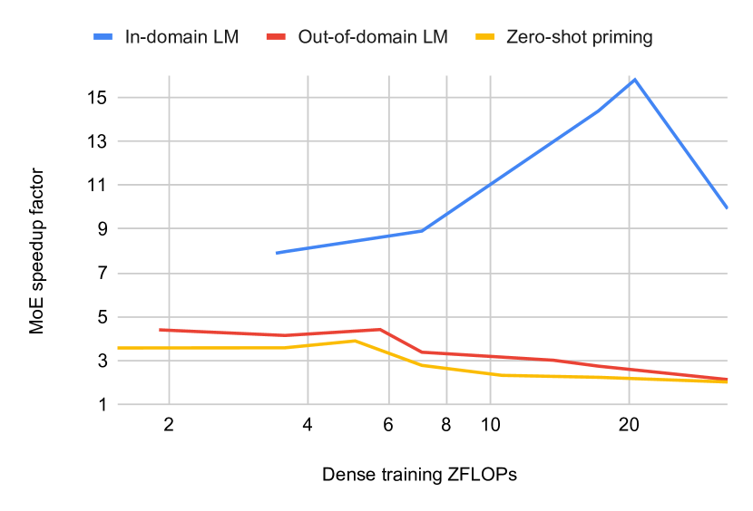
Figure 1: Estimate of how much more efficient MoEs are relative to dense models. A speedup factor of $y$ indicates that an MoE model can match the performance of the corresponding dense model—trained with $x$ ZFLOPs—using $y$ times less compute (i.e., $x/y$ ZFLOPs). We estimate this factor according to validation perplexity for in-domain language modeling, the Pile perplexity for out-of-domain language modeling, and average accuracy across 6 tasks for zero-shot priming. See §3.3.3 for more details.

Sparse models allow for increased number of learnable parameters without the associated computational costs. For example, sparsely gated mixture of experts (MoE) Lepikhin et al. (2021) have been successfully used for language modeling and machine translation (Lepikhin et al., 2021; Lewis et al., 2021; Roller et al., 2021), but are yet to be shown effective for fine-tuning Fedus et al. (2021) as well as zero- and few-shot learning. We hypothesize that sparse models are comparatively accurate to dense models but at a much lower computational footprint. To measure this claim, we train traditional dense and MoE language models ranging in size from several hundred million parameters to more than one trillion parameters and present a careful empirical comparison of these models on downstream tasks in zero-shot, few-shot and fully supervised settings.

As shown in Figure 1, we find that MoE models can indeed achieve similar downstream task performance as dense models at a fraction of the compute. For models with relatively modest compute budgets, a MoE model can perform on par with a dense model that requires almost four times as much compute. Downstream task performance improves with scale for both MoE models and dense models. While we observe that the performance gap narrows as we increase model size, even at larger compute budgets ($\sim$ 5000 GPU days), our largest MoE model (1.1T parameters) outperforms a dense model with similar computational cost (6.7B parameters). We further compare and contrast the performance of dense and sparse models with similar computational signatures and observe some performance variations across tasks and domains, suggesting this an interesting area for future research. In summary, our contributions are:

• We present a comprehensive study of sparse models for zero and few-shot learning at scale;

• We demonstrate that even at scale sparse MoE models can yield competitive zero and few-shot performance at a fraction of the computation for model training and inference;

• We observe some differences in how dense and sparse models generalize at scale suggesting complementary behaviour that could be an interesting future research direction.

2 Background and Related Work

2.1 Large Language Models / GPT-3

Progress in the field of NLP has been driven by increasingly large Language Models (LMs) pretrained on large text datasets. While numerous variations have been proposed, such LMs are predominantly based on the transformer architecture (Vaswani et al., 2017). Models are pretrained by hiding parts of the input: predicting the next word sequentially left-to-right, masking words in the text (Devlin et al., 2019; Liu et al., 2019), or perturbing and/or masking spans (Lewis et al., 2020; Raffel et al., 2020). The resulting models can be quickly adapted to perform new tasks at high accuracy by fine-tuning on supervised data (Devlin et al., 2019; Liu et al., 2019).

Recently, GPT-3 (Brown et al., 2020) demonstrated that large LMs can perform zero- and few-shot learning without fine-tuning through in-context learning. Notably, many of these in-context zero- and few-shot learning behaviors emerge or amplify at scale. Concurrent to our work, Rae et al. (2022) and Smith et al. (2022) further explore scaling dense language models.

2.2 Sparse models

One drawback of dense model scaling is that it grows increasingly computationally expensive. To more efficiently increase model capacity, conditional compute strategies have been developed (Bengio et al., 2013; Davis and Arel, 2013; Cho and Bengio, 2014; Bengio et al., 2015), where each input activates a subset of the model. Recent work (Lewis et al., 2021; Lepikhin et al., 2021; Fedus et al., 2021; Fan et al., 2021) has studied different conditional compute strategies that work well with Transformer models for natural language tasks. In this work, we focus on Sparsely Gated Mixture of Expert (MoE) models (Shazeer et al., 2017; Lepikhin et al., 2021). Sparse MoE models replace the dense feed forward network block in every alternate Transformer layer with an MoE layer. The MoE layer has a routing gate that learns which tokens are to be mapped to which set of experts (we use top-2 experts). To ensure scalability and training efficiency, it is also common to include a weighted gate loss term as in Lepikhin et al. (2021) to the cross entropy loss to encourage the tokens to be uniformly distributed to the experts. Concurrent to our work, Du et al. (2021), Rajbhandari et al. (2022) and Clark et al. (2022) also study MoE scaling.

GPT-3 (dense)						Ours (dense)						Ours (MoE)
size	cost	$l$	$h$	$e$		size	cost	$l$	$h$	$e$		size	cost	$l$	$h$	$e$
125M	0.36	12	768	–		125M	0.36	12	768	–		15B	0.43	12	768	512
355M	1.06	24	1024	–		355M	1.06	24	1024	–		52B	1.30	24	1024	512
760M	2.13	24	1536	–		—						—
1.3B	3.57	24	2048	–		1.3B	3.57	24	2048	–		207B	4.53	24	2048	512
2.7B	7.08	32	2560	–		2.7B	7.08	32	2560	–		—
6.7B	17.12	32	4096	–		6.7B	17.12	32	4096	–		1.1T	22.27	32	4096	512
13B	32.67	40	5120	–		13B	32.67	40	5120	–		—
175B	430.17	96	12288	–		—						—

Table 1: Dense and mixture of expert (MoE) model details. size: number of parameters, cost: training ZFLOPs, $l$: layers, $h$: hidden dimension, $e$: number of experts. All models are trained for 300B tokens with a sequence length of 2048 tokens. Models within the same row are roughly comparable. We estimate the training cost in ZFLOPs analytically (see Appendix G).

2.3 Zero-shot and Few-shot Learning

Recent works (Schick and Schütze, 2021a; Radford et al., 2019) have directly evaluated LMs on unseen tasks successfully (zero-shot learning), by recasting their task inputs as cloze-style prompt completion tasks. This is in contrast to the traditional approach of augmenting LMs with task-specific heads, followed by supervised fine-tuning (Devlin et al., 2019; Raffel et al., 2020). Subsequently, Brown et al. (2020) demonstrated that priming LMs with a few input-output examples (few-shot learning) before careful prompting can improve task performance, that grows with model scale without any fine-tuning, and this gave rise to new resources for prompt engineering (Bach et al., 2022). In this paper, we contrast the zero-shot, few-shot, and fully supervised fine-tuning performance of dense and MoE models. Finally, Schick and Schütze (2021b) perform few-shot learning by few-shot fine-tuning using pattern-exploiting training, whose efficiency can be improved by performing partial fine-tuning of a small number of additional task-specific parameters instead (Lester et al., 2021; Li and Liang, 2021; Houlsby et al., 2019).

2.4 Large-scale training

Many of the models we consider in this work are too big to be trained using standard data parallel techniques, since parameter storage would exceed the usable memory of a single GPU. We adopt several techniques to make these models feasible to train, including pure FP16 training, activation checkpointing and fully sharded data parallel training. These techniques are described in more depth in Appendix F.

3 Experimental Setup

3.1 Models

We train autoregressive (decoder-only) transformer models that roughly match the sizes and architecture explored in Brown et al. (2020). Model sizes are summarized in Table 1. We use pre-normalization transformer blocks (Baevski and Auli, 2019; Child et al., 2019) and GELU activations (Hendrycks and Gimpel, 2016). We differ from Brown et al. (2020) in two ways: (1) we use only dense attention, while they alternate between dense and locally banded sparse attention; and (2) we train our models with sinusoidal positional embeddings, following Shortformer Press et al. (2020).

We also train MoE models that mirror our dense model configurations (see the third set of columns in Table 1), so that comparisons are approximately matched in terms of the number of floating point operations (FLOPs). Our MoE models follow the design proposed in Lepikhin et al. (2021) with alternating dense and expert layers and top-2 expert selection. We use 512 experts in each expert layer ($E=512$). Each expert has a capacity of $\frac{C\cdot B}{E}$ tokens, where $C$ is a capacity factor that we set to $2$ and $B$ is the total batch size in tokens. Capacity refers to the maximum number of tokens that are routed to each expert. Once an expert is at capacity for a given batch, additional tokens are considered to be “overflowed" with their representations passed-through via the residual connection.

Fedus et al. (2021) report instability training large MoE models and suggest rescaling the initial model weights, which we do not find necessary. We instead observe that expert parameters have an $E$-times smaller batch size relative to dense (data parallel) parameters and accordingly rescale expert gradients by a factor $\frac{1}{\sqrt{E}}$. This rescaling aligns with theory suggesting that an $E$-times increase in batch size should be accompanied by a $\sqrt{E}$ increase in learning rate (Krizhevsky, 2014).

Following Brown et al. (2020), we train our models for 300B tokens with a context size (sequence length) of 2048 tokens. The batch size and learning rate are set according to the model size following Brown et al. (2020). We linearly warm-up the learning rate from $0$ over the first 375M tokens and linearly decay back to $0$ over the remaining tokens. We use the Adam optimizer Kingma and Ba (2015) with $\beta_{1}=0.9$, $\beta_{2}=0.98$, $\epsilon=10^{-8}$, weight decay of 0.01 and dropout of 0.1.

We train our models in PyTorch Paszke et al. (2017) using fairseq (Ott et al., 2019).

3.2 Pretraining data

We pretrain our models on a union of six English-language datasets, including the five datasets used to pretrain RoBERTa (Liu et al., 2019) and the English subset of CC100, totalling 112B tokens corresponding to 453GB:

• BookCorpus (Zhu et al., 2019) consists of more than 10K unpublished books (4GB);

• English Wikipedia, excluding lists, tables and headers (12GB);

• CC-News (Nagel, 2016) contains 63 millions English news articles crawled between September 2016 and February 2019 (76GB);

• OpenWebText (Gokaslan and Cohen, 2019), an open source recreation of the WebText dataset used to train GPT-2 (38GB);

• CC-Stories (Trinh and Le, 2018) contains a subset of CommonCrawl data filtered to match the story-like style of Winograd schemas (31GB);

• English CC100 (Wenzek et al., 2020), a dataset extracted from CommonCrawl snapshots between January 2018 and December 2018, filtered to match the style of Wikipedia (292GB).

We encode our data using the same Byte-Pair Encoding (BPE) as GPT-2 (Radford et al., 2019) and RoBERTa (Liu et al., 2019) with a vocabulary of 50K subword units.

3.3 Evaluation

We evaluate models in terms of their in-domain and out-of-domain perplexity, as well as downstream task performance.

3.3.1 Perplexity Evaluation

We first evaluate our models on their ability to predict the next token in a sequence as measured by perplexity. Similar to training, we concatenate all documents in a given dataset using empty lines as separators, split the resulting sequence into non-overlapping blocks of 2048 tokens, and score each block independently.

We evaluate and report perplexity in both in-domain and out-of-domain settings. In-domain, we sample a held-out subset of the combined pretraining data (§3.2). For out-of-domain we use data from The Pile (Gao et al., 2021), a public dataset that combines data from 22 diverse sources (e.g., ArXiv, Github, OpenSubtitles, etc.). We report perplexities on the official test set of each individual subset, as well as the average across all subsets.

3.3.2 Downstream Evaluation

We target models that can perform downstream tasks well. Recent work shows that good perplexity performance does not always align with good performance on downstream tasks Tay et al. (2021). Hence, we evaluate our models accordingly.

Benchmarks.

We evaluate our models on a subset of the tasks considered in Brown et al. (2020). As GPT-3 performance varies greatly across tasks and model sizes, we focus on tasks for which GPT-3 either demonstrated consistent gains from scaling, or consistent gains going from zero-shot to few-shot settings.

Few-shot: we use WinoGrande (Sakaguchi et al., 2020), StoryCloze (Mostafazadeh et al., 2016) and OpenBookQA (Mihaylov et al., 2018), the only non-generation tasks for which Brown et al. (2020) reported meaningful gains over zero-shot at our scale. We exclude SuperGLUE, since we were not able to reproduce results reported in Brown et al. (2020) using the public GPT-3 API.

Zero-shot: in addition to the 3 few-shot tasks, we evaluate on ReCoRD (Zhang et al., 2018), HellaSwag (Zellers et al., 2019) and PIQA (Bisk et al., 2020). Brown et al. (2020) reported strong results and monotonic improvements from scaling on these tasks.

Evaluation protocol.

Following Brown et al. (2020), we report results on the development set for all tasks except OpenBookQA and StoryCloze, for which we use the test set. For few-shot learning, we report the average results across 25 runs, randomly sampling a different set of few-shot examples from the training set each time. For priming, we further shuffle the few-shot examples for each test instance. Following Brown et al. (2020), we use k=50 few-shot examples for WinoGrande, k=70 for StoryCloze and k=100 for OpenBookQA. In cases where this exceeds the maximum context length for the model, we truncate the prompt keeping the maximum number of full examples that fit.

Baselines.

We compare to the published GPT-3 numbers (Brown et al., 2020) as our primary baseline. To validate our experimental framework, we also evaluate GPT-3 leveraging the OpenAI API using our own evaluation code and settings. Unfortunately, the correspondence between model sizes and model names in the OpenAI API is not published. We follow other published work (Gao et al., 2021) and guess the correspondence based on our results from the public API as compared to results in Brown et al. (2020) (see §4.2.1).

Methods.

We compare both priming and fine-tuning-based approaches.

• Priming: We use a language model to separately score each label choice using the same templates as Brown et al. (2020), and pick the one with the highest score. For few-shot learning, we use a single newline to separate examples. Our scoring function follows the description in Brown et al. (2020):

  • For WinoGrande, we take the log-likelihood of the common suffix of the different candidates.

  • For OpenBookQA, we normalize by the unconditional probability of each candidate by taking $\frac{p(\mathtt{completion}|\mathtt{context})}{p(\mathtt{completion}|\mathtt{answer\_context})}$, where we use the string “Answer: ” as answer_context.

  • For ReCoRD, we take the sum of per-token log-probabilities.

  • For all the other tasks, we take the average of per-token log-probabilities, ignoring the common prefix of the different candidates.

• Fine-tuning: Although supervised fine-tuning of pre-trained LMs on task specific training data, $\mathcal{D}$, requires updating and storage of all model parameters per task, the process typically produces significant task specific performance improvements. We contrast the fine-tuning performance of sparse models and their dense counterparts following Radford et al. (2018), which applies an additional task-specific linear layer $W_{y}$ on the representation from the final transformer block for each input candidate separately, followed by a softmax layer. We fine-tune all model parameters using the entire training set (fully supervised learning). In addition to our zero-shot tasks, we also evaluate on 3 widely-used classification tasks: BoolQ (Clark et al., 2019), MNLI (Williams et al., 2018) and SST-2 (Socher et al., 2013). More details are in Appendix B.

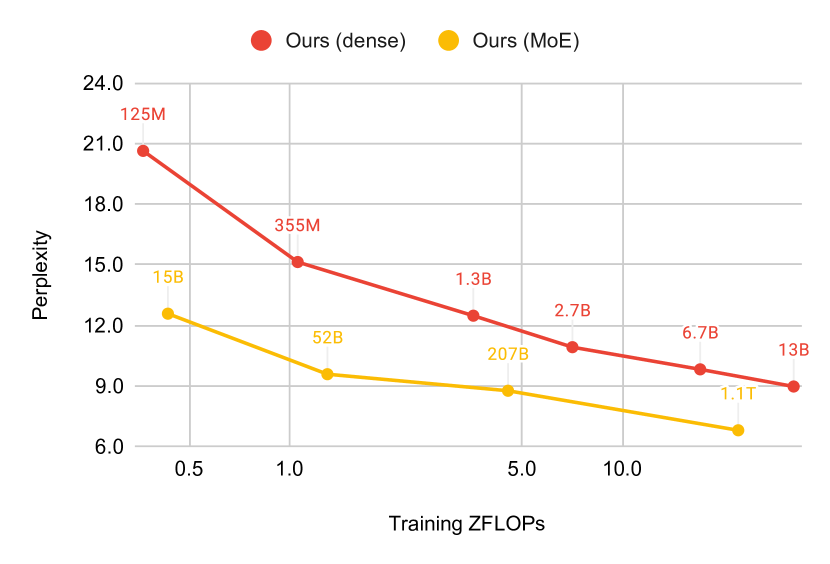
(a) In-domain (validation)

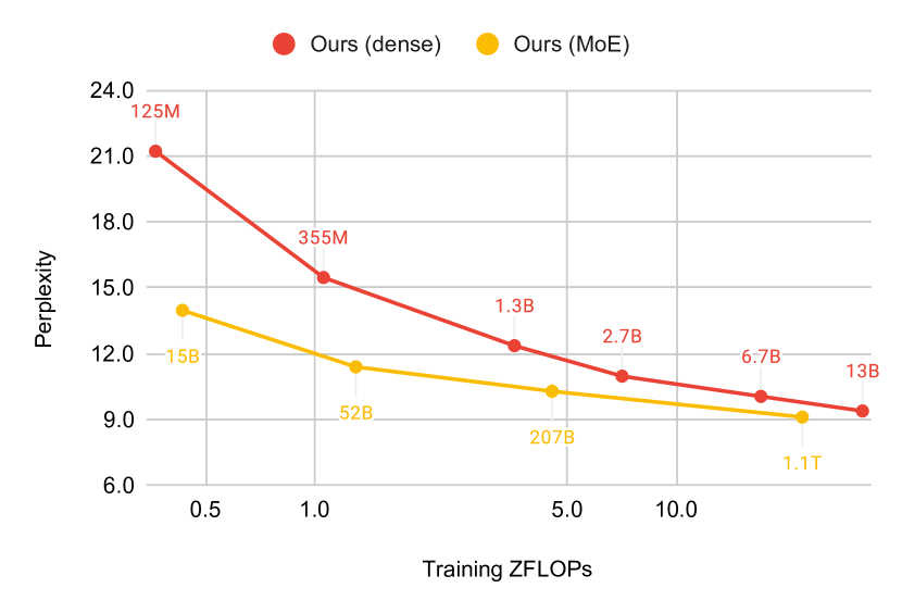
(b) Out-of-domain (the Pile)

Figure 2: Language modeling perplexity. For the Pile, we report the average perplexity across the 22 subsets.

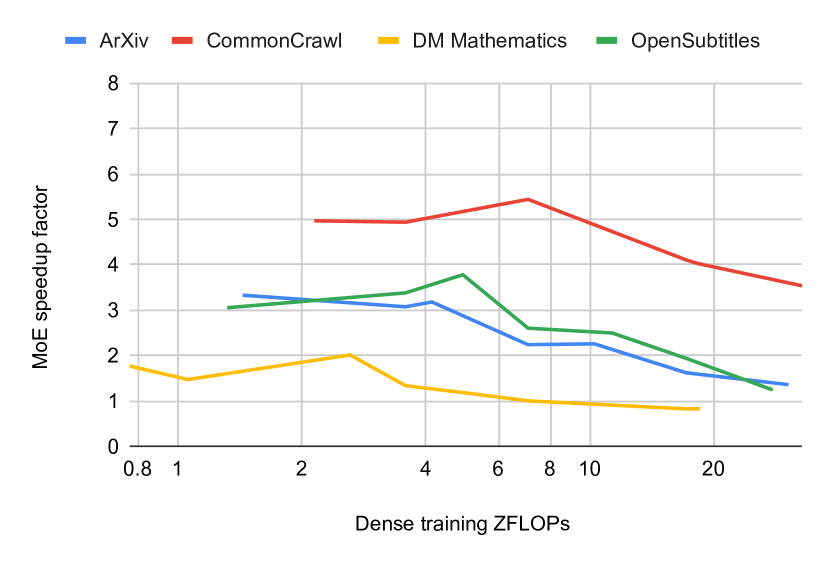
(a) Language modeling (the Pile)

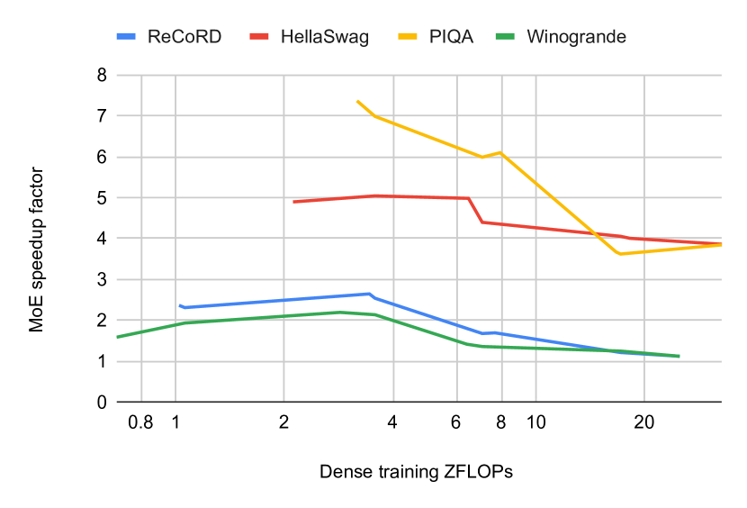
(b) Zero-shot priming

Figure 3: Estimate of how much more efficient MoEs are relative to dense models in representative datasets. A speedup factor of $y$ indicates that an MoE model can match the performance of the corresponding dense model using $y$ times less compute. Refer to §3.3.3 for more details.

3.3.3 MoE speedup factor

We hypothesize that sparse models can achieve comparable performance at a smaller compute budget. As such, it is informative to measure how much more efficient MoEs are at achieving a specific performance level relative to dense models. We estimate how many FLOPs $\operatorname{c}(t)$ the model needs to achieve performance $t$ in a particular task (as measured by perplexity for language modeling and accuracy for downstream tasks) using either an MoE or a dense model. Given that we only have discrete observations, we estimate exact missing values by interpolating on a logarithmic scale as follows:

$$\operatorname{c}(t)=\exp\left(\log\operatorname{c}_{lo}(t)+r\left(\log\operatorname{c}_{hi}(t)-\log\operatorname{c}_{lo}(t)\right)\right)$$

where $r=\frac{t-t_{lo}}{t_{hi}-t_{lo}}$, $t_{lo}$ and $t_{hi}$ are the closest performance to $t$ from the available models while being lower and higher than $t$, respectively, and $\operatorname{c}_{lo}(t)$ and $\operatorname{c}_{hi}$ are their corresponding training cost in ZFLOPs.

The interpolation gives us matching performance levels for dense and MoE models. We use them to compute the MoE speedup factor $\operatorname{c}_{dense}(t)/\operatorname{c}_{moe}(t)$. For example, if a dense model requiring 20 ZFLOPs achieves a performance of $90\%$ on a given task and a MoE model requiring 5 ZFLOPs achieves the same performance, then the formula produces saving factor of 4. We visualize the savings curve using $\operatorname{c}_{dense}(t)$ in the $x$ axis, which allows us to contrast speedup in different tasks in a comparable scale.

		RE	HS	PI	WG	SC	OB	avg
GPT-3 (paper)	125M	70.8	33.7	64.6	52.0	63.3	35.6	53.3
	355M	78.5	43.6	70.2	52.1	68.5	43.2	59.4
	760M	82.1	51.0	72.9	57.4	72.4	45.2	63.5
	1.3B	84.1	54.7	75.1	58.7	73.4	46.8	65.5
	2.7B	86.2	62.8	75.6	62.3	77.2	53.0	69.5
	6.7B	88.6	67.4	78.0	64.5	77.7	50.4	71.1
	13B	89.0	70.9	78.5	67.9	79.5	55.6	73.6
	175B	90.2	78.9	81.0	70.2	83.2	57.6	76.9
GPT-3 (API)	ada	77.4	42.9	70.3	52.9	68.6	41.0	58.9
	babb.	83.1	55.1	74.5	59.4	73.3	45.6	65.2
	curie	87.1	67.8	77.1	64.3	77.7	50.8	70.8
	davi.	–	78.8	80.0	70.0	83.1	58.8	–
Ours (dense)	125M	69.3	33.7	65.3	52.1	66.0	35.4	53.6
	355M	78.1	46.2	70.6	54.2	71.0	42.0	60.4
	1.3B	83.5	58.4	74.6	58.1	76.8	49.4	66.8
	2.7B	85.8	65.9	76.6	61.4	78.2	49.6	69.6
	6.7B	87.5	70.2	78.2	64.7	80.5	51.8	72.2
	13B	88.5	73.7	79.0	67.6	80.9	55.4	74.2
Ours (MoE)	15B	77.8	53.2	74.3	53.4	73.6	42.0	62.4
	52B	83.4	64.9	76.8	57.4	75.9	51.0	68.2
	207B	86.0	70.5	78.2	60.9	78.1	50.8	70.7
	1.1T	88.0	78.6	80.3	66.4	81.8	55.2	75.0

Table 2: Zero-shot priming accuracy. GPT-3 (paper) results taken from Brown et al. (2020), all the other results were obtained by us as described in §3.3.2. RE: ReCoRD, HS: HellaSwag, PI: PIQA, WG: WinoGrande, SC: StoryCloze, OB: OpenBookQA. We do not evaluate the largest GPT-3 model (davinci) on RE given the high price.

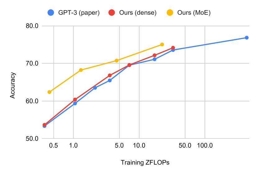
Figure 4: Zero-shot priming accuracy averaged across 6 tasks as a function of compute cost. Each point corresponds to a different, fully-trained model (see Table 1). GPT-3 (paper) results taken from Brown et al. (2020).

4 Results and Analysis

4.1 Language modeling perplexity

We report our perplexity results in Figure 2, and visualize the speedup curves in representative subsets of the Pile (Gao et al., 2021) in Figure 3(a). Refer to Appendix A for full results for all the 22 subsets of the Pile.

We observe that all MoE models outperform their dense counterparts in all datasets, but their advantage greatly varies across domains and models. MoEs are most efficient when evaluated in-domain, where they are able to match the performance of dense models trained with 8-16x more compute (see Figure 1). The improvement is more modest in out-of-domain settings, bringing a speedup of 2-4 on the Pile. This is reflected in Figure 2, where the gap between the MoE and dense curves is substantially smaller in out-of-domain settings. Moreover, the advantage of MoEs over dense models decreases at scale: MoEs need $\sim$4 times less compute to match the performance of dense models trained with 2-6 ZFLOPs, but the speedup is $\sim$2 for dense models trained with $\sim$30 ZFLOPs.

We also observe large difference across the subsets of the Pile, which correspond to different domains. As shown in Figure 3(a), MoEs obtain the largest speedups in subsets that are closest to the training corpus (e.g., CommonCrawl). The efficiency gains are more moderate but still remarkable for other domains like ArXiv and OpenSubtitles. Our largest MoE model barely outperforms its dense counterpart on DM Mathematics (7.63 vs. 7.66 perplexity), which is arguably very different from the training domain.

4.2 Downstream task evaluation

4.2.1 Zero-shot learning

We report zero-shot results in Table 2, and visualize how the different model families scale in Figure 4.

Our dense models perform at par with their GPT-3 counterparts. This is consistent across different tasks, with our models doing marginally better on average. We are thus able to match Brown et al. (2020) despite some notable differences in our setup (e.g., different training corpus), establishing a solid baseline to evaluate MoE models on downstream tasks. Similarly, when using our own code to evaluate the strongest GPT-3 API backend (davinci), we obtain numbers that replicate those reported in the original paper for their largest model, which reinforces that our evaluation settings are comparable to Brown et al. (2020).

As with language modeling, MoEs outperform their dense counterparts for all datasets and model sizes. But, once again, we find the advantage narrows at scale as illustrated in Figure 4. Similar to the domain differences in language modeling, we observe differences across downstream tasks. As shown in Figure 3(b), MoEs obtain significant speedups in certain tasks like HellaSwag and PIQA, but this improvement is more modest in other tasks such as ReCoRD and Winogrande.

4.2.2 Few-shot learning

We report our few-shot results in Table 3 and plot the corresponding improvement over zero-shot in Figure 5.

Our dense baselines perform at par or slightly better than GPT-3. We observe that the improvement over zero-shot is bigger for larger models, further supporting that certain capabilities in language models emerge at scale (Brown et al., 2020). Finally, we find that our larger MoE models also benefit from few-shot learning, outperforming their dense counterparts in all conditions. However, the improvements going from zero-shot to few-shot are smaller for MoE models compared to their dense counterparts. For example, the average for the 6.7B dense model improves by 3.6 points to 69.3 going from zero-shot to few-shot, whereas the corresponding 1.1T model improves by 2.3 points yielding 70.1.

		WG	SC	OB	avg
GPT-3 (paper)	125M	51.3 –0.7	62.3 –1.0	37.0 +1.4	50.2 –0.1
	355M	52.6 +0.5	70.2 +1.7	43.6 +0.4	55.5 +0.9
	760M	57.5 +0.1	73.9 +1.5	48.0 +2.8	59.8 +1.5
	1.3B	59.1 +0.4	76.1 +2.7	50.6 +3.8	61.9 +2.3
	2.7B	62.6 +0.3	80.2 +3.0	55.6 +2.6	66.1 +2.0
	6.7B	67.4 +2.9	81.2 +3.5	55.2 +4.8	67.9 +3.7
	13B	70.0 +2.1	83.0 +3.5	60.8 +5.2	71.3 +3.6
	175B	77.7 +7.5	87.7 +4.5	65.4 +7.8	76.9 +6.6
Ours (dense)	125M	52.2 +0.1	64.7 –1.3	35.0 –0.4	50.7 –0.5
	355M	53.7 –0.5	72.2 +1.1	42.0 +0.0	56.0 +0.2
	1.3B	60.1 +2.0	78.6 +1.9	49.4 +0.0	62.7 +1.3
	2.7B	63.9 +2.5	82.1 +3.8	53.2 +3.6	66.4 +3.3
	6.7B	67.6 +2.9	83.2 +2.7	57.0 +5.2	69.3 +3.6
	13B	71.0 +3.5	85.0 +4.1	59.5 +4.1	71.8 +3.9
Ours (MoE)	15B	52.5 –0.9	71.4 –2.1	42.2 +0.2	55.4 –0.9
	52B	58.1 +0.7	77.5 +1.6	48.9 –2.1	61.5 +0.1
	207B	62.8 +1.9	81.1 +3.0	52.4 +1.6	65.4 +2.2
	1.1T	68.6 +2.3	83.9 +2.1	57.7 +2.5	70.1 +2.3

Table 3: Few-shot priming accuracy and absolute improvement over zero-shot. GPT-3 (paper) results taken from Brown et al. (2020), all the other results were obtained by us as described in §3.3.2. WG: WinoGrande, SC: StoryCloze, OB: OpenBookQA.

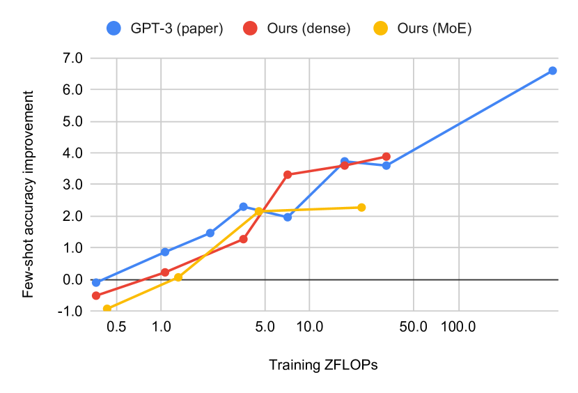
Figure 5: Absolute accuracy improvement going from zero-shot to few-shot, averaged across 3 tasks. Each point corresponds to a different, fully-trained model (see Table 1). GPT-3 (paper) results taken from Brown et al. (2020).

4.2.3 Supervised Fine-Tuning

Table 4 contrasts full fine-tuning performance of MoE models with their dense counterparts on 8 datasets, using zero-shot accuracy as a baseline for reference. We did not fine-tune the 6.7B and 13B dense models and the 1.1T MoE models, owing to their high resource needs. As expected, supervised fine-tuning yields substantial performance benefits for all dense models across all datasets, over zero-shot performance. In contrast, although fine-tuning of MoE models produces substantial benefits for Storycloze, BoolQ, SST-2, MNLI and some improvements on OpenBookQA, it results in worse performance for HellaSwag, PIQA, and Winogrande. For the cases where we see improvements, the accuracy of fine-tuned MoE models approach that of their corresponding dense models. For this comparison, we fine-tune MoE models exactly as we do the dense models. While MoE models may benefit from alternative fine-tuning approaches, for example, selective fine-tuning of the expert or non-expert parameters, we leave such exploration to future work.

		Ours (Dense)				Ours (MoE)
		125M	355M	1.3B	2.7B	15B	52B	207B
SC	zero-shot	66.0	71.0	76.8	78.2	73.6	75.9	78.1
	fine-tune	87.8	89.5	93.8	97.0	80.3	84.9	80.9
OB	zero-shot	35.4	42.0	49.4	49.6	42.0	51.0	50.8
	fine-tune	50.6	59.0	67.4	70.8	51.2	51.4	51.0
BQ	zero-shot	56.1	58.6	58.7	60.3	60.9	56.0	54.2
	fine-tune	73.2	75.2	79.6	84.6	71.6	75.3	77.5
MN	zero-shot	46.2	52.1	55.3	56.0	49.3	52.1	52.6
	fine-tune	80.9	84.3	84.1	88.9	77.7	81.2	78.7
SST-2	zero-shot	50.9	50.9	51.6	51.9	51.6	50.9	50.9
	fine-tune	92.9	92.9	94.8	93.4	89.3	90.1	90.3
HS	zero-shot	33.7	46.2	58.4	65.9	53.2	64.9	70.5
	fine-tune	50.7	64.8	74.1	90.0	37.3	45.4	42.2
PI	zero-shot	65.3	70.6	74.6	76.6	74.3	76.8	78.2
	fine-tune	68.2	71.7	71.2	80.3	66.3	66.1	68.3
WG	zero-shot	52.1	54.2	58.1	61.4	53.4	57.4	60.9
	fine-tune	65.7	63.3	67.4	69.5	50.2	56.0	50.4

Table 4: Fully supervised fine-tuning accuracy compared with zero-shot accuracy. SC: StoryCloze, OB: OpenBookQA, BQ: BoolQ, MN: MNLI, HS: HellaSwag, PI: PIQA, WG: WinoGrande. Largest models omitted owing to their high resource utilization.

5 Conclusion

We present results for scaling sparse Language Models up to 1.1T parameters. We observe that up to this scale sparse models offer better performance vs. computation trade-off when compared to their dense counterparts for language modeling, zero- and few-shot learning. While the gap begins to close at scale our biggest sparse model outperforms its dense counterpart where the latter requires twice as much computation. These results confirm that sparse MoE models can provide an alternative to widely used dense architectures that saves computation and reduces model energy consumption.

Ethical considerations

Previous work Sheng et al. (2019); Bordia and Bowman (2019); Nadeem et al. (2021); de Vassimon Manela et al. (2021) has observed that language models absorb bias and toxicity represented in the training data. So as to better understand the potential harms of our models in this front, we evaluated them on StereoSet Nadeem et al. (2021) and CrowS-Pairs Nangia et al. (2020), and report our results in Appendix C. Our results show that the percentage of bias and stereotype in dense and MoE models is comparable, especially at scale. Moreover, in general, we note worse performance (more bias/stereotyping) at larger scales. This observation points to more research needed in order to mitigate such behavior. Intuitively however, we believe that sparse models may be inherently more controllable – e.g. designing specific experts – than dense models. We leave this line of investigation for future research.

Another concern of scaling language models is the energy usage and the associated environmental impact required for training, which we discuss in detail in Appendix D. Nevertheless, our work shows that MoEs can be a more compute-efficient alternative to traditional dense models, which could alleviate the environmental impact of future scaling efforts. Moreover, by releasing all of our pre-trained language models, we believe we have alleviated some exploration burden for the community and the environment, allowing for more efficient offsets for other researchers.

In the spirit of transparency and allowing for maximal replicability and accountability, we include data and model cards together with our code.

Limitations

Our study is limited to one specific MoE configuration. In particular, our sparse and dense models use the same hyperparameters and model structure, closely following GPT-3. However, it is possible that this configuration is suboptimal for scaling MoE models. Similarly, we did not explore different MoE-specific hyperparameters, such as the number of experts. Finally, while our work reveals that the performance gap between MoE and dense models varies greatly across tasks and domains, the specific factors that make certain tasks more favorable for MoEs remain unclear.

			Dense							MoE
			125M	355M	1.3B	2.7B	6.7B	13B		15B	52B	207B	1.1T
In-domain	Validation		20.65	15.14	12.48	10.92	9.82	8.97		12.58	9.58	8.76	6.80
Out-of-domain — (The Pile)	ArXiv		15.74	11.42	9.00	8.03	7.29	6.86		10.81	8.79	7.72	6.91
	Bibliotik		26.78	19.62	15.75	13.96	12.81	11.96		17.80	14.64	13.29	11.88
	BookCorpus		23.60	17.91	14.83	13.36	12.38	11.70		16.54	13.90	12.82	11.57
	CommonCrawl		22.49	16.92	13.91	12.47	11.50	10.80		15.17	12.47	11.43	10.02
	DM_Mathematics		12.29	9.73	8.51	8.10	7.66	7.41		10.51	8.82	8.28	7.63
	Enron_Emails		19.98	15.71	12.32	11.40	10.78	10.09		14.24	12.18	11.08	10.45
	EuroParl		27.16	15.80	12.02	9.91	8.63	7.68		12.58	9.47	8.41	6.92
	FreeLaw		16.78	11.98	9.44	8.33	7.58	7.08		10.54	8.49	7.68	6.84
	Github		8.92	6.55	5.13	4.61	4.30	4.03		6.11	4.93	4.41	3.99
	Gutenberg_PG-19		29.15	20.70	16.39	14.37	13.03	12.08		18.85	14.94	13.48	11.90
	HackerNews		29.37	22.53	18.11	16.20	14.96	14.08		20.72	17.15	15.67	14.21
	NIH_ExPorter		26.78	19.18	15.28	13.55	12.40	11.64		17.08	14.00	12.66	11.42
	OpenSubtitles		20.72	16.87	14.16	13.05	12.28	11.61		16.38	13.64	12.64	11.78
	OpenWebText2		20.56	14.64	11.88	10.47	9.51	8.79		12.76	10.03	9.03	7.06
	PhilPapers		27.60	20.00	15.99	14.07	12.90	12.03		18.77	15.19	13.56	11.91
	PubMed_Abstracts		24.16	16.56	12.95	11.38	10.35	9.65		14.46	11.71	10.49	9.36
	PubMed_Central		12.19	9.35	7.65	6.89	6.36	6.03		8.74	7.32	6.60	6.02
	StackExchange		17.76	12.46	9.65	8.43	7.58	7.04		10.99	8.74	7.73	6.72
	USPTO		17.15	12.85	10.43	9.36	8.67	8.18		12.00	9.95	9.01	8.14
	Ubuntu_IRC		28.40	21.47	16.16	13.92	12.50	11.48		17.80	14.79	12.85	11.49
	Wikipedia_en		20.51	14.61	11.59	10.22	9.22	8.56		12.35	9.68	8.60	6.65
	YoutubeSubtitles		19.01	13.51	10.80	9.31	8.38	7.70		12.23	9.88	8.80	7.51
	Average		21.23	15.47	12.36	10.97	10.05	9.39		13.97	11.40	10.28	9.11

Table 5: Full perplexity results.

Appendix A Full perplexity results

Table 5 reports the full perplexity results, including all the different subsets of the Pile.

Appendix B Fine-tuning Settings

We run fine-tuning for a fixed number of epochs (100 for BoolQ, OpenBookQA, StoryCloze, and PIQA, 25 for HellaSwag, Winogrande, and SST-2, 6 for MNLI) and perform model selection based on validation set accuracy. For datasets either without a validation set or where we evaluate on the validation set, we randomly split the training set and use 80% for fine-tuning and 20% for per-epoch validation.

Appendix C Understanding Potential Harms

Previous work Sheng et al. (2019); Bordia and Bowman (2019); Nadeem et al. (2021); de Vassimon Manela et al. (2021) has observed that language models absorb bias and toxicity represented in the training data. We set out to explore if sparse models would behave differently than dense models in this arena. To that end, we evaluate our dense and MoE models on two popular benchmarks: StereoSet Nadeem et al. (2021) and CrowS-Pairs Nangia et al. (2020). StereoSet measures bias across four domains: profession, gender, religion, and race. CrowS-Pairs dataset covers nine bias types: race, gender/gender identity, sexual orientation, religion, age, nationality, disability, physical appearance, and socioeconomic status.

Stereotypical bias as a function of scale.

Table 6 presents the results on StereoSet benchmark using three metrics: (1) Language Modeling Score (LMS): defined as the percentage of instances in which a language model prefers meaningful over meaningless associations (higher LMS is better); (2) Stereotype Score (SS): defined as the percentage of instances where a model prefers a stereotypical association over an anti-stereotypical association (SS score close to $50$ is better, while a more biased model would have a higher score towards $100\%$); (3) Idealized CAT Score (ICAT): defined as a combination of LMS and SS to capture both in a single metric: ${\scriptstyle LMS}*\frac{min(SS,100-SS)}{50}$ (higher ICAT is better).

Table 7 presents the performance of our models on CrowS-Pairs using the Stereotype Score (SS) metric. Similar to StereoSet, we observe that both dense and MoE models get worse with scale, again with statistically significant ($p<0.05$) difference between best and worst scores based on bootstrap test Noreen (1989); Efron and Tibshirani (1994).

		Ours (Dense)					Ours (MoE)
Category		125M	355M	1.3B	2.7B	6.7B	15B	52B	207B	1.1T
Prof.	LMS	80.8	82.0	81.9	80.8	79.3	79.7	80.5	81.1	78.0
	SS	48.2	49.8	51.3	53.6	54.2	52.2	54.9	54.8	54.4
	ICAT	77.9	81.7	79.8	75.1	72.6	76.2	72.6	73.4	71.1
Gender	LMS	83.3	82.4	83.9	83.1	82.2	81.4	82.9	82.2	80.2
	SS	59.9	59.1	59.1	60.7	60.3	58.7	58.3	58.7	61.2
	ICAT	66.7	67.4	68.6	65.2	65.2	67.3	69.2	68.0	62.3
Reli.	LMS	85.9	87.8	87.2	87.2	85.3	87.8	85.9	83.3	81.4
	SS	50.0	46.2	50.0	55.1	52.6	50.0	48.7	51.3	51.3
	ICAT	85.9	81.1	87.2	78.2	80.9	87.8	83.7	81.2	79.3
Race	LMS	82.3	82.3	83.8	83.0	83.1	83.7	83.4	82.0	82.1
	SS	42.9	45.7	48.3	49.8	50.3	47.1	47.3	49.7	47.5
	ICAT	70.7	75.2	80.8	82.7	82.6	78.9	79.0	81.5	78.0
Overall	LMS	82.0	82.4	83.2	82.3	81.6	82.1	82.3	81.7	80.2
	SS	47.2	48.8	50.7	52.7	53.0	50.5	51.6	52.8	51.9
	ICAT	77.4	80.5	82.0	77.9	76.6	81.2	79.7	77.2	77.2

Table 6: Stereotypical bias comparison on the inter-sentence task of StereoSet. Note that for LMS and ICAT higher is better whereas for SS closer to $50$ is better. All scores are macro averages of all samples present in a category. Overall represents all the samples in this dataset.

	Ours (Dense)					Ours (MoE)
Category	125M	355M	1.3B	2.7B	6.7B	15B	52B	207B	1.1T
Gender	56.5	58.4	56.5	58.0	60.3	56.9	63.4	62.2	60.7
Religion	63.8	67.6	68.6	70.5	73.3	64.8	68.6	70.5	73.3
Race/Color	61.1	58.7	63.8	62.0	67.6	57.4	59.7	60.5	61.8
Sexual orientation	78.6	78.6	82.1	76.2	79.8	73.8	78.6	78.6	76.2
Age	57.5	60.9	60.9	62.1	62.1	66.7	59.8	66.7	66.7
Nationality	46.5	47.2	61.0	54.7	59.1	52.2	56.6	61.6	57.2
Disability	66.7	70.0	75.0	71.7	70.0	75.0	73.3	75.0	76.7
Physical appearance	73.0	65.1	69.8	71.4	74.6	71.4	71.4	74.6	79.4
Socioeconomic status	69.2	66.9	72.7	68.0	71.5	69.8	69.8	72.1	73.3
Overall	61.3	60.9	65.1	63.4	67.0	61.4	63.9	65.5	65.7

Table 7: Stereotypical bias comparison on CrowS-Pairs. Scores closer to $50$ are better. All scores are macro averages.

Stereotypical bias in dense vs MoE models.

We observe that as the model size increases, both dense and MoE models get worse ICAT scores in general – they become more biased with a statistically significant difference between best and worst scores. On the StereoSet benchmark, corresponding dense and sparse models (comparable FLOPs) yield comparable performance. On the CrowS-Pairs MoE models perform slightly better (less biased) than dense models on average but the difference is not statistically significant (see Table 6 and Table 7).

Appendix D CO2 Emission Related to Experiments

	GPU days	tCO2e
125M dense	26	0.1
355M dense	77	0.2
1.3B dense	258	0.8
2.7B dense	512	1.7
6.7B dense	1238	4.0
13B dense	2363	7.7
15B MoE	43	0.1
52B MoE	131	0.4
207B MoE	456	1.5
1.1T MoE	2241	7.3
Total	7345	23.8
GShard 600B MoE		4.8
Switch Transformer 1.5T MoE		72.2
GPT-3 175B		552.1

Table 8: Estimated training time and energy costs to train the models reported in this paper, based on the number of A100 GPU-days required for training. See Appendix D for more details about these estimates.

The carbon emissions of the experiments reported in this work are dominated by the largest models, in particular the 13B parameter dense and 1.1T parameter MoE models. We trained our largest models on Azure NDv4 instances with A100 GPUs (TDP of 400W) in the West US 2 region, which has a carbon efficiency of 0.3 kgCO₂e/kWh and assumed Power Usage Effectiveness (PUE) of 1.125. Thus each GPU-day of training is responsible for 3.24 kgCO₂e of emissions, of which 100 percent is directly offset by the cloud provider.

In Table 8 we report training time and energy usage for our models based on the above estimates, as well as estimates from Patterson et al. (2021) for other large-scale LMs, in particular GShard (Lepikhin et al., 2021), Switch Transformer (Fedus et al., 2021) and GPT-3 (Brown et al., 2020). Training times (GPU days) are computed assuming a throughput of 160 TFLOP/s and 115 TFLOP/s per A100 GPU for our dense and MoE models, respectively, based on observed training speeds for our largest models.

We note that these estimates do not account for the costs associated with manufacturing the infrastructure to train such models, which can be significant (Gupta et al., 2021; Wu et al., 2021). We also note that these estimates do not account for pilot experiments common in the early exploratory stages of a research project. We estimate that pilot experimentation adds a factor of 2 to the total training cost, since most exploration and tuning is performed at small scale where compute costs are small, and the largest models are typically trained at most once or twice. For instance, we trained and discarded a pilot 6.7B dense and 1.1T MoE model in the early stages of this project, but trained the 13B dense model once.

Appendix E Knowledge Distillation

Teacher size	Cost	PPL
None (Baseline)	0.36	16.01
MoE 15B	0.43	15.20
355M Dense	1.06	14.88
1.3B Dense	3.57	14.67
MoE 52B	1.30	14.64
2.7B Dense	7.08	14.62

Table 9: Distillation Results. Cost refers to the cost to train the teacher model (see Table 1). PPL is the in-domain validation perplexity.

In Section 3.3.3 we show that sparse (MoE) models are significantly more efficient to train than dense models. However, inference for large sparse models can be challenging, since the large number of parameters (most of which are inactive) introduce significant storage costs compared to dense models.

In this section we explore whether it is possible to blend the benefits of dense and sparse models via knowledge distillation (Hinton et al., 2015). Building on recent work in this area (Shleifer and Rush, 2020; Sanh et al., 2020; Fedus et al., 2021), we train small dense “student” models to mimic the behavior of larger “teacher” models, which may be either large dense or large sparse (MoE) models.

Methods

We train dense student models with 12 layers and hidden dimension 768, matching the 125M dense model architecture in Table 1. We use a weighted training objective that combines the standard cross entropy loss (25% weight) with a soft distillation loss (75% weight) that encourages the student model to reproduce the logits of the teacher. Additionally, we use a reduced sequence length of 1024 tokens to speed up experimentation.

Results

We report results in Table 9. We find that student models trained with knowledge distillation improve over a well tuned dense baseline for both dense and sparse teacher models. Furthermore, some of the efficiency advantages of sparse training can be transmitted to a dense student through distillation. For example, student models distilled from a 52B parameter MoE teacher outperform student models distilled from a 1.3B parameter dense teacher, despite that the dense teacher model is twice as costly to train.

Appendix F Techniques for Large-scale Training

We adopt several techniques to train models in this work, including a more memory-efficient recipe for FP16 training, activation checkpointing and Fully Sharded Data Parallel.

FP16 Training:

Typical mixed-precision training recipes require storing model weights in both 16-bit (FP16) and 32-bit (FP32), as well as storing optimizer state in 32-bit to preserve accurate weight updates (Micikevicius et al., 2018; Ott et al., 2018). Thus training a model in mixed precision with Adam requires 16 bytes of memory per parameter to maintain 16-bit and 32-bit weights (6 bytes), Adam optimizer state (8 bytes) and gradients (2 bytes), not including any memory required for activations.

In practice we find we can reduce memory requirements by 50% by maintaining only 16-bit model weights, optimizer state and gradients with no loss in model accuracy. First, we simply discard the 32-bit model weights, saving 4 bytes per parameter, since pilot experiments showed this to have no impact on model quality when training with large batch sizes. Second, the Adam optimizer state can be stored in 16-bit by dynamically rescaling the values to avoid underflow. Specifically, we compute the standard Adam weight update in 32-bit and then apply the following transformation at the end of each optimization step to maintain the optimizer state in 16-bit (Dhariwal et al., 2020):

$$\vec{m}_{fp16}=\frac{\vec{m}}{\frac{\max abs(\vec{m})}{\textrm{FLOAT16\_MAX}}+\epsilon}$$

where $\epsilon=10^{-8}$ and $\textrm{{FLOAT16\_MAX}}=65504.0$ is the largest finite value expressible in FP16. We apply this transformation separately for the first and second moment estimates in Adam.

Activation Checkpointing:

Activation size grows proportionally to the model and batch size, making it infeasible to store activations for transformer models with more than a couple of billion parameters. We adopt a popular technique called activation checkpointing, which saves memory during training by discarding a subset of activations in the forward pass and recomputing them in the backward pass (Chen et al., 2016). This technique results in a 33% increase in computation, but can often reduce activation memory requirements by a factor of 10 (Rajbhandari et al., 2020). In our experiments we only store activations between transformer layers and recompute intermediate activations within each layer during the backward pass.

Fully Sharded Data Parallel:

In data parallel training, gradients are averaged across multiple workers (GPUs) that process distinct partitions of the data. Standard implementations maintain redundant copies of the model weights and optimizer state on each GPU, however this wastes GPU memory and makes it challenging to scale the model size beyond what can fit on a single GPU. Recent work has explored sharding model parameters, optimizer state and gradients across workers (Xu et al., 2020; Rajbhandari et al., 2020), enabling training of models with more than one trillion parameters using only data parallelism without the added complexity introduced by model parallel training approaches like pipeline or tensor parallelism (Huang et al., 2019; Shoeybi et al., 2019; Narayanan et al., 2021).

We implement these ideas in Fully Sharded Data Parallel (FSDP), which shards model parameters in-place and gathers the parameters on all workers just-in-time for the forward and backward pass. Training with FSDP is typically faster than standard data parallel implementations for three reasons: (1) sharding reduces the cost of the optimizer step and weight update by distributing it across workers, rather than redundantly updating model replicas on each worker; (2) while FSDP introduces 50% more communication, this extra communication is overlapped with the computation in the forward and backward pass; and (3) FSDP yields significant memory savings, which can be used to increase the batch size and achieve higher GPU utilization.

One important decision when using FSDP is choosing which submodules in the model to “wrap" with FSDP. If the wrapping is too fine-grained, then the parameter shards will be very small which reduces communication efficiency. If the wrapping is too coarse, then this increases the peak resident memory and may pose challenges when scaling to larger model sizes. In this work we wrap every transformer layer with FSDP, which ensures a reasonably large message size for communication while still limiting the peak resident memory to the size of a single layer.

Appendix G Counting FLOPs

We count the number of floating-point operations (FLOPs) analytically following Narayanan et al. (2021). We assume that all models are trained with activation checkpointing and thus have an additional forward pass before the backward pass. Thus the total training FLOPs for our dense models is given by:

$$F_{\textrm{dense}}=96Tlh^{2}\left(1+\frac{s}{6h}+\frac{V}{16lh}\right),$$

where $T$ is the total number of training tokens, $l$ is the number of layers, $h$ is the hidden dimension, $s$ is the sequence length and $V$ is the vocabulary size. In this work, $T=300e^{9}$, $s=2048$ and $V=51200$ for all models.

For mixture of expert models, we account for an additional feed-forward network at every other layer for the top-2 routing in GShard Lepikhin et al. (2021), and ignore the FLOPs of the routing projection which is negligible. The resulting training FLOPs for our MoE models is given by:

$$F_{\textrm{MoE}}=F_{\textrm{dense}}+32Tlh^{2}.$$

Notably, this quantity is independent of the number of experts.

References

- Bach et al. (2022) Stephen H Bach, Victor Sanh, Zheng-Xin Yong, Albert Webson, Colin Raffel, Nihal V Nayak, Abheesht Sharma, Taewoon Kim, M Saiful Bari, Thibault Fevry, et al. 2022. Promptsource: An integrated development environment and repository for natural language prompts. arXiv preprint arXiv:2202.01279.
- Baevski and Auli (2019) Alexei Baevski and Michael Auli. 2019. Adaptive input representations for neural language modeling. In International Conference on Learning Representations.
- Bender et al. (2021) Emily M Bender, Timnit Gebru, Angelina McMillan-Major, and Shmargaret Shmitchell. 2021. On the dangers of stochastic parrots: Can language models be too big? In Proceedings of the 2021 ACM Conference on Fairness, Accountability, and Transparency, pages 610–623.
- Bengio et al. (2015) Emmanuel Bengio, Pierre-Luc Bacon, Joelle Pineau, and Doina Precup. 2015. Conditional computation in neural networks for faster models. arXiv preprint arXiv:1511.06297.
- Bengio et al. (2013) Yoshua Bengio, Nicholas Léonard, and Aaron Courville. 2013. Estimating or propagating gradients through stochastic neurons for conditional computation. arXiv preprint arXiv:1308.3432.
- Bergman (2021) Sara Bergman. 2021. How Can I Calculate CO2eq emissions for my Azure VM?
- Bisk et al. (2020) Yonatan Bisk, Rowan Zellers, Ronan Le bras, Jianfeng Gao, and Yejin Choi. 2020. Piqa: Reasoning about physical commonsense in natural language. Proceedings of the AAAI Conference on Artificial Intelligence, 34(05):7432–7439.
- Blodgett et al. (2021) Su Lin Blodgett, Gilsinia Lopez, Alexandra Olteanu, Robert Sim, and Hanna Wallach. 2021. Stereotyping norwegian salmon: an inventory of pitfalls in fairness benchmark datasets. In Proceedings of the 59th Annual Meeting of the Association for Computational Linguistics and the 11th International Joint Conference on Natural Language Processing (Volume 1: Long Papers), pages 1004–1015.
- Bordia and Bowman (2019) Shikha Bordia and Samuel Bowman. 2019. Identifying and reducing gender bias in word-level language models. In Proceedings of the 2019 Conference of the North American Chapter of the Association for Computational Linguistics: Student Research Workshop, pages 7–15.
- Brown et al. (2020) Tom Brown, Benjamin Mann, Nick Ryder, Melanie Subbiah, Jared D Kaplan, Prafulla Dhariwal, Arvind Neelakantan, Pranav Shyam, Girish Sastry, Amanda Askell, Sandhini Agarwal, Ariel Herbert-Voss, Gretchen Krueger, Tom Henighan, Rewon Child, Aditya Ramesh, Daniel Ziegler, Jeffrey Wu, Clemens Winter, Chris Hesse, Mark Chen, Eric Sigler, Mateusz Litwin, Scott Gray, Benjamin Chess, Jack Clark, Christopher Berner, Sam McCandlish, Alec Radford, Ilya Sutskever, and Dario Amodei. 2020. Language models are few-shot learners. In Advances in Neural Information Processing Systems, volume 33, pages 1877–1901. Curran Associates, Inc.
- Chen et al. (2016) Tianqi Chen, Bing Xu, Chiyuan Zhang, and Carlos Guestrin. 2016. Training deep nets with sublinear memory cost. arXiv preprint arXiv:1604.06174.
- Child et al. (2019) Rewon Child, Scott Gray, Alec Radford, and Ilya Sutskever. 2019. Generating long sequences with sparse transformers. arXiv preprint arXiv:1904.10509.
- Cho and Bengio (2014) Kyunghyun Cho and Yoshua Bengio. 2014. Exponentially increasing the capacity-to-computation ratio for conditional computation in deep learning. arXiv preprint arXiv:1406.7362.
- Clark et al. (2022) Aidan Clark, Diego de las Casas, Aurelia Guy, Arthur Mensch, Michela Paganini, Jordan Hoffmann, Bogdan Damoc, Blake Hechtman, Trevor Cai, Sebastian Borgeaud, George van den Driessche, Eliza Rutherford, Tom Hennigan, Matthew Johnson, Katie Millican, Albin Cassirer, Chris Jones, Elena Buchatskaya, David Budden, Laurent Sifre, Simon Osindero, Oriol Vinyals, Jack Rae, Erich Elsen, Koray Kavukcuoglu, and Karen Simonyan. 2022. Unified scaling laws for routed language models.
- Clark et al. (2019) Christopher Clark, Kenton Lee, Ming-Wei Chang, Tom Kwiatkowski, Michael Collins, and Kristina Toutanova. 2019. BoolQ: Exploring the surprising difficulty of natural yes/no questions. In Proceedings of the 2019 Conference of the North American Chapter of the Association for Computational Linguistics: Human Language Technologies, Volume 1 (Long and Short Papers), pages 2924–2936, Minneapolis, Minnesota. Association for Computational Linguistics.
- Davis and Arel (2013) Andrew Davis and Itamar Arel. 2013. Low-rank approximations for conditional feedforward computation in deep neural networks. arXiv preprint arXiv:1312.4461.
- de Vassimon Manela et al. (2021) Daniel de Vassimon Manela, David Errington, Thomas Fisher, Boris van Breugel, and Pasquale Minervini. 2021. Stereotype and skew: Quantifying gender bias in pre-trained and fine-tuned language models. In Proceedings of the 16th Conference of the European Chapter of the Association for Computational Linguistics: Main Volume, pages 2232–2242.
- Devlin et al. (2019) Jacob Devlin, Ming-Wei Chang, Kenton Lee, and Kristina Toutanova. 2019. BERT: Pre-training of deep bidirectional transformers for language understanding. In North American Association for Computational Linguistics (NAACL).
- Dhariwal et al. (2020) Prafulla Dhariwal, Heewoo Jun, Christine Payne, Jong Wook Kim, Alec Radford, and Ilya Sutskever. 2020. Jukebox: A generative model for music. arXiv preprint arXiv:2005.00341.
- Du et al. (2021) Nan Du, Yanping Huang, Andrew M. Dai, Simon Tong, Dmitry Lepikhin, Yuanzhong Xu, Maxim Krikun, Yanqi Zhou, Adams Wei Yu, Orhan Firat, Barret Zoph, Liam Fedus, Maarten Bosma, Zongwei Zhou, Tao Wang, Yu Emma Wang, Kellie Webster, Marie Pellat, Kevin Robinson, Kathy Meier-Hellstern, Toju Duke, Lucas Dixon, Kun Zhang, Quoc V Le, Yonghui Wu, Zhifeng Chen, and Claire Cui. 2021. Glam: Efficient scaling of language models with mixture-of-experts.
- Efron and Tibshirani (1994) Bradley Efron and Robert J Tibshirani. 1994. An introduction to the bootstrap. CRC press.
- Fan et al. (2021) Angela Fan, Shruti Bhosale, Holger Schwenk, Zhiyi Ma, Ahmed El-Kishky, Siddharth Goyal, Mandeep Baines, Onur Celebi, Guillaume Wenzek, Vishrav Chaudhary, et al. 2021. Beyond english-centric multilingual machine translation. Journal of Machine Learning Research, 22(107):1–48.
- Fedus et al. (2021) William Fedus, Barret Zoph, and Noam Shazeer. 2021. Switch transformers: Scaling to trillion parameter models with simple and efficient sparsity. arXiv preprint arXiv:2101.03961.
- Gao et al. (2021) Leo Gao, Stella Biderman, Sid Black, Laurence Golding, Travis Hoppe, Charles Foster, Jason Phang, Horace He, Anish Thite, Noa Nabeshima, Shawn Presser, and Connor Leahy. 2021. The pile: An 800gb dataset of diverse text for language modeling. CoRR, abs/2101.00027.
- Gokaslan and Cohen (2019) Aaron Gokaslan and Vanya Cohen. 2019. Openwebtext corpus.
- Gupta et al. (2021) Udit Gupta, Young Geun Kim, Sylvia Lee, Jordan Tse, Hsien-Hsin S Lee, Gu-Yeon Wei, David Brooks, and Carole-Jean Wu. 2021. Chasing carbon: The elusive environmental footprint of computing. IEEE International Symposium on High-Performance Computer Architecture (HPCA 2021).
- Hendrycks and Gimpel (2016) Dan Hendrycks and Kevin Gimpel. 2016. Gaussian error linear units (gelus). arXiv preprint arXiv:1606.08415.
- Hinton et al. (2015) Geoffrey Hinton, Oriol Vinyals, and Jeff Dean. 2015. Distilling the knowledge in a neural network. arXiv preprint arXiv:1503.02531.
- Houlsby et al. (2019) Neil Houlsby, Andrei Giurgiu, Stanislaw Jastrzebski, Bruna Morrone, Quentin De Laroussilhe, Andrea Gesmundo, Mona Attariyan, and Sylvain Gelly. 2019. Parameter-efficient transfer learning for nlp. In International Conference on Machine Learning, pages 2790–2799. PMLR.
- Huang et al. (2019) Yanping Huang, Youlong Cheng, Ankur Bapna, Orhan Firat, Dehao Chen, Mia Chen, HyoukJoong Lee, Jiquan Ngiam, Quoc V Le, Yonghui Wu, et al. 2019. Gpipe: Efficient training of giant neural networks using pipeline parallelism. Advances in neural information processing systems, 32:103–112.
- Kingma and Ba (2015) Diederik Kingma and Jimmy Ba. 2015. Adam: A method for stochastic optimization. In International Conference on Learning Representations (ICLR).
- Krizhevsky (2014) Alex Krizhevsky. 2014. One weird trick for parallelizing convolutional neural networks. arXiv preprint arXiv:1404.5997.
- Lacoste et al. (2019) Alexandre Lacoste, Alexandra Luccioni, Victor Schmidt, and Thomas Dandres. 2019. Quantifying the carbon emissions of machine learning. arXiv preprint arXiv:1910.09700.
- Lan et al. (2020) Zhenzhong Lan, Mingda Chen, Sebastian Goodman, Kevin Gimpel, Piyush Sharma, and Radu Soricut. 2020. Albert: A lite bert for self-supervised learning of language representations. In International Conference on Learning Representations (ICLR).
- Lepikhin et al. (2021) Dmitry Lepikhin, HyoukJoong Lee, Yuanzhong Xu, Dehao Chen, Orhan Firat, Yanping Huang, Maxim Krikun, Noam Shazeer, and Zhifeng Chen. 2021. GShard: Scaling giant models with conditional computation and automatic sharding. In International Conference on Learning Representations (ICLR).
- Lester et al. (2021) Brian Lester, Rami Al-Rfou, and Noah Constant. 2021. The power of scale for parameter-efficient prompt tuning. In Proceedings of the 2021 Conference on Empirical Methods in Natural Language Processing, pages 3045–3059.
- Lewis et al. (2021) Mike Lewis, Shruti Bhosale, Tim Dettmers, Naman Goyal, and Luke Zettlemoyer. 2021. Base layers: Simplifying training of large, sparse models. In ICML.
- Lewis et al. (2020) Mike Lewis, Yinhan Liu, Naman Goyal, Marjan Ghazvininejad, Abdelrahman Mohamed, Omer Levy, Veselin Stoyanov, and Luke Zettlemoyer. 2020. BART: Denoising sequence-to-sequence pre-training for natural language generation, translation, and comprehension. In Proceedings of the 58th Annual Meeting of the Association for Computational Linguistics, pages 7871–7880, Online. Association for Computational Linguistics.
- Li and Liang (2021) Xiang Lisa Li and Percy Liang. 2021. Prefix-tuning: Optimizing continuous prompts for generation. In Proceedings of the 59th Annual Meeting of the Association for Computational Linguistics and the 11th International Joint Conference on Natural Language Processing (Volume 1: Long Papers), pages 4582–4597.
- Liu et al. (2019) Yinhan Liu, Myle Ott, Naman Goyal, Jingfei Du, Mandar Joshi, Danqi Chen, Omer Levy, Mike Lewis, Luke Zettlemoyer, and Veselin Stoyanov. 2019. Roberta: A robustly optimized bert pretraining approach. arXiv preprint arXiv:1907.11692.
- Micikevicius et al. (2018) Paulius Micikevicius, Sharan Narang, Jonah Alben, Gregory Diamos, Erich Elsen, David Garcia, Boris Ginsburg, Michael Houston, Oleksii Kuchaiev, Ganesh Venkatesh, and Hao Wu. 2018. Mixed precision training. In International Conference on Learning Representations.
- Mihaylov et al. (2018) Todor Mihaylov, Peter Clark, Tushar Khot, and Ashish Sabharwal. 2018. Can a suit of armor conduct electricity? a new dataset for open book question answering. In Proceedings of the 2018 Conference on Empirical Methods in Natural Language Processing, pages 2381–2391, Brussels, Belgium. Association for Computational Linguistics.
- Mostafazadeh et al. (2016) Nasrin Mostafazadeh, Nathanael Chambers, Xiaodong He, Devi Parikh, Dhruv Batra, Lucy Vanderwende, Pushmeet Kohli, and James Allen. 2016. A corpus and cloze evaluation for deeper understanding of commonsense stories. In Proceedings of the 2016 Conference of the North American Chapter of the Association for Computational Linguistics: Human Language Technologies, pages 839–849, San Diego, California. Association for Computational Linguistics.
- Nadeem et al. (2021) Moin Nadeem, Anna Bethke, and Siva Reddy. 2021. StereoSet: Measuring stereotypical bias in pretrained language models. In Association for Computational Linguistics (ACL).
- Nagel (2016) Sebastian Nagel. 2016. Cc-news.
- Nangia et al. (2020) Nikita Nangia, Clara Vania, Rasika Bhalerao, and Samuel R. Bowman. 2020. CrowS-pairs: A challenge dataset for measuring social biases in masked language models. In Proceedings of the 2020 Conference on Empirical Methods in Natural Language Processing (EMNLP), pages 1953–1967, Online. Association for Computational Linguistics.
- Narayanan et al. (2021) Deepak Narayanan, Mohammad Shoeybi, Jared Casper, Patrick LeGresley, Mostofa Patwary, Vijay Anand Korthikanti, Dmitri Vainbrand, Prethvi Kashinkunti, Julie Bernauer, Bryan Catanzaro, et al. 2021. Efficient large-scale language model training on gpu clusters. arXiv preprint arXiv:2104.04473.
- Noreen (1989) Eric W Noreen. 1989. Computer-intensive methods for testing hypotheses. Wiley New York.
- Ott et al. (2019) Myle Ott, Sergey Edunov, Alexei Baevski, Angela Fan, Sam Gross, Nathan Ng, David Grangier, and Michael Auli. 2019. fairseq: A fast, extensible toolkit for sequence modeling. In North American Association for Computational Linguistics (NAACL): System Demonstrations.
- Ott et al. (2018) Myle Ott, Sergey Edunov, David Grangier, and Michael Auli. 2018. Scaling neural machine translation. In Proceedings of the Third Conference on Machine Translation (WMT).
- Paszke et al. (2017) Adam Paszke, Sam Gross, Soumith Chintala, Gregory Chanan, Edward Yang, Zachary DeVito, Zeming Lin, Alban Desmaison, Luca Antiga, and Adam Lerer. 2017. Automatic differentiation in PyTorch. In NIPS Autodiff Workshop.
- Patterson et al. (2021) David Patterson, Joseph Gonzalez, Quoc Le, Chen Liang, Lluis-Miquel Munguia, Daniel Rothchild, David So, Maud Texier, and Jeff Dean. 2021. Carbon emissions and large neural network training. arXiv preprint arXiv:2104.10350.
- Peters et al. (2018) Matthew Peters, Mark Neumann, Mohit Iyyer, Matt Gardner, Christopher Clark, Kenton Lee, and Luke Zettlemoyer. 2018. Deep contextualized word representations. In North American Association for Computational Linguistics (NAACL).
- Press et al. (2020) Ofir Press, Noah A Smith, and Mike Lewis. 2020. Shortformer: Better language modeling using shorter inputs. arXiv preprint arXiv:2012.15832.
- Radford et al. (2018) Alec Radford, Karthik Narasimhan, Time Salimans, and Ilya Sutskever. 2018. Improving language understanding with unsupervised learning. Technical report, OpenAI.
- Radford et al. (2019) Alec Radford, Jeffrey Wu, Rewon Child, David Luan, Dario Amodei, and Ilya Sutskever. 2019. Language models are unsupervised multitask learners. Technical report, OpenAI.
- Rae et al. (2022) Jack W. Rae, Sebastian Borgeaud, Trevor Cai, Katie Millican, Jordan Hoffmann, Francis Song, John Aslanides, Sarah Henderson, Roman Ring, Susannah Young, Eliza Rutherford, Tom Hennigan, Jacob Menick, Albin Cassirer, Richard Powell, George van den Driessche, Lisa Anne Hendricks, Maribeth Rauh, Po-Sen Huang, Amelia Glaese, Johannes Welbl, Sumanth Dathathri, Saffron Huang, Jonathan Uesato, John Mellor, Irina Higgins, Antonia Creswell, Nat McAleese, Amy Wu, Erich Elsen, Siddhant Jayakumar, Elena Buchatskaya, David Budden, Esme Sutherland, Karen Simonyan, Michela Paganini, Laurent Sifre, Lena Martens, Xiang Lorraine Li, Adhiguna Kuncoro, Aida Nematzadeh, Elena Gribovskaya, Domenic Donato, Angeliki Lazaridou, Arthur Mensch, Jean-Baptiste Lespiau, Maria Tsimpoukelli, Nikolai Grigorev, Doug Fritz, Thibault Sottiaux, Mantas Pajarskas, Toby Pohlen, Zhitao Gong, Daniel Toyama, Cyprien de Masson d’Autume, Yujia Li, Tayfun Terzi, Vladimir Mikulik, Igor Babuschkin, Aidan Clark, Diego de Las Casas, Aurelia Guy, Chris Jones, James Bradbury, Matthew Johnson, Blake Hechtman, Laura Weidinger, Iason Gabriel, William Isaac, Ed Lockhart, Simon Osindero, Laura Rimell, Chris Dyer, Oriol Vinyals, Kareem Ayoub, Jeff Stanway, Lorrayne Bennett, Demis Hassabis, Koray Kavukcuoglu, and Geoffrey Irving. 2022. Scaling language models: Methods, analysis & insights from training gopher.
- Raffel et al. (2020) Colin Raffel, Noam Shazeer, Adam Roberts, Katherine Lee, Sharan Narang, Michael Matena, Yanqi Zhou, Wei Li, and Peter J Liu. 2020. Exploring the limits of transfer learning with a unified text-to-text transformer. The Journal of Machine Learning Research (JMLR), 21:1–67.
- Rajbhandari et al. (2022) Samyam Rajbhandari, Conglong Li, Zhewei Yao, Minjia Zhang, Reza Yazdani Aminabadi, Ammar Ahmad Awan, Jeff Rasley, and Yuxiong He. 2022. Deepspeed-moe: Advancing mixture-of-experts inference and training to power next-generation ai scale.
- Rajbhandari et al. (2020) Samyam Rajbhandari, Jeff Rasley, Olatunji Ruwase, and Yuxiong He. 2020. Zero: Memory optimizations toward training trillion parameter models. In SC20: International Conference for High Performance Computing, Networking, Storage and Analysis, pages 1–16. IEEE.
- Roller et al. (2021) Stephen Roller, Sainbayar Sukhbaatar, Arthur Szlam, and Jason Weston. 2021. Hash layers for large sparse models. arXiv preprint arXiv:2106.04426.
- Sakaguchi et al. (2020) Keisuke Sakaguchi, Ronan Le Bras, Chandra Bhagavatula, and Yejin Choi. 2020. Winogrande: An adversarial winograd schema challenge at scale. Proceedings of the AAAI Conference on Artificial Intelligence, 34(05):8732–8740.
- Sanh et al. (2020) Victor Sanh, Lysandre Debut, Julien Chaumond, and Thomas Wolf. 2020. Distilbert, a distilled version of bert: smaller, faster, cheaper and lighter.
- Schick and Schütze (2021a) Timo Schick and Hinrich Schütze. 2021a. Exploiting cloze-questions for few-shot text classification and natural language inference. In Proceedings of the 16th Conference of the European Chapter of the Association for Computational Linguistics: Main Volume, pages 255–269, Online. Association for Computational Linguistics.
- Schick and Schütze (2021b) Timo Schick and Hinrich Schütze. 2021b. It’s not just size that matters: Small language models are also few-shot learners. In Proceedings of the 2021 Conference of the North American Chapter of the Association for Computational Linguistics: Human Language Technologies, pages 2339–2352.
- Schwartz et al. (2019) Roy Schwartz, Jesse Dodge, Noah A Smith, and Oren Etzioni. 2019. Green ai. arXiv preprint arXiv:1907.10597.
- Shazeer et al. (2017) Noam Shazeer, Azalia Mirhoseini, Krzysztof Maziarz, Andy Davis, Quoc Le, Geoffrey Hinton, and Jeff Dean. 2017. Outrageously large neural networks: The sparsely-gated mixture-of-experts layer. arXiv preprint arXiv:1701.06538.
- Sheng et al. (2019) Emily Sheng, Kai-Wei Chang, Premkumar Natarajan, and Nanyun Peng. 2019. The woman worked as a babysitter: On biases in language generation. In Proceedings of the 2019 Conference on Empirical Methods in Natural Language Processing and the 9th International Joint Conference on Natural Language Processing (EMNLP-IJCNLP).
- Shleifer and Rush (2020) Sam Shleifer and Alexander M. Rush. 2020. Pre-trained summarization distillation.
- Shoeybi et al. (2019) Mohammad Shoeybi, Mostofa Patwary, Raul Puri, Patrick LeGresley, Jared Casper, and Bryan Catanzaro. 2019. Megatron-lm: Training multi-billion parameter language models using model parallelism. arXiv preprint arXiv:1909.08053.
- Smith et al. (2022) Shaden Smith, Mostofa Patwary, Brandon Norick, Patrick LeGresley, Samyam Rajbhandari, Jared Casper, Zhun Liu, Shrimai Prabhumoye, George Zerveas, Vijay Korthikanti, Elton Zhang, Rewon Child, Reza Yazdani Aminabadi, Julie Bernauer, Xia Song, Mohammad Shoeybi, Yuxiong He, Michael Houston, Saurabh Tiwary, and Bryan Catanzaro. 2022. Using deepspeed and megatron to train megatron-turing nlg 530b, a large-scale generative language model.
- Socher et al. (2013) Richard Socher, Alex Perelygin, Jean Wu, Jason Chuang, Christopher D. Manning, Andrew Ng, and Christopher Potts. 2013. Recursive deep models for semantic compositionality over a sentiment treebank. In Proceedings of the 2013 Conference on Empirical Methods in Natural Language Processing, pages 1631–1642, Seattle, Washington, USA. Association for Computational Linguistics.
- Strubell et al. (2019) Emma Strubell, Ananya Ganesh, and Andrew McCallum. 2019. Energy and policy considerations for deep learning in nlp. arXiv preprint arXiv:1906.02243.
- Tay et al. (2021) Yi Tay, Mostafa Dehghani, Jinfeng Rao, William Fedus, Samira Abnar, Hyung Won Chung, Sharan Narang, Dani Yogatama, Ashish Vaswani, and Donald Metzler. 2021. Scale efficiently: Insights from pre-training and fine-tuning transformers. arXiv preprint arXiv:2109.10686.
- Trinh and Le (2018) Trieu H Trinh and Quoc V Le. 2018. A simple method for commonsense reasoning. arXiv preprint arXiv:1806.02847.
- Vaswani et al. (2017) Ashish Vaswani, Noam Shazeer, Niki Parmar, Jakob Uszkoreit, Llion Jones, Aidan N Gomez, Łukasz Kaiser, and Illia Polosukhin. 2017. Attention is all you need. In Advances in neural information processing systems.
- Wenzek et al. (2020) Guillaume Wenzek, Marie-Anne Lachaux, Alexis Conneau, Vishrav Chaudhary, Francisco Guzmán, Armand Joulin, and Edouard Grave. 2020. CCNet: Extracting high quality monolingual datasets from web crawl data. In Proceedings of the 12th Language Resources and Evaluation Conference, pages 4003–4012, Marseille, France. European Language Resources Association.
- Williams et al. (2018) Adina Williams, Nikita Nangia, and Samuel Bowman. 2018. A broad-coverage challenge corpus for sentence understanding through inference. In Proceedings of the 2018 Conference of the North American Chapter of the Association for Computational Linguistics: Human Language Technologies, Volume 1 (Long Papers), pages 1112–1122, New Orleans, Louisiana. Association for Computational Linguistics.
- Wu et al. (2021) Carole-Jean Wu, Ramya Raghavendra, Udit Gupta, Bilge Acun, Newsha Ardalani, Kiwan Maeng, Gloria Chang, Fiona Aga Behram, James Huang, Charles Bai, et al. 2021. Sustainable ai: Environmental implications, challenges and opportunities. arXiv preprint arXiv:2111.00364.
- Xu et al. (2020) Yuanzhong Xu, HyoukJoong Lee, Dehao Chen, Hongjun Choi, Blake Hechtman, and Shibo Wang. 2020. Automatic cross-replica sharding of weight update in data-parallel training. arXiv preprint arXiv:2004.13336.
- Zellers et al. (2019) Rowan Zellers, Ari Holtzman, Yonatan Bisk, Ali Farhadi, and Yejin Choi. 2019. HellaSwag: Can a machine really finish your sentence? In Proceedings of the 57th Annual Meeting of the Association for Computational Linguistics, pages 4791–4800, Florence, Italy. Association for Computational Linguistics.
- Zhang et al. (2018) Sheng Zhang, Xiaodong Liu, Jingjing Liu, Jianfeng Gao, Kevin Duh, and Benjamin Van Durme. 2018. ReCoRD: Bridging the gap between human and machine commonsense reading comprehension. arXiv preprint 1810.12885.
- Zhu et al. (2019) Yukun Zhu, Ryan Kiros, Richard Zemel, Ruslan Salakhutdinov, Raquel Urtasun, Antonio Torralba, and Sanja Fidler. 2019. Aligning books and movies: Towards story-like visual explanations by watching movies and reading books. arXiv preprint arXiv:1506.06724.