How to assess the primordial origin of single gravitational-wave events
with mass, spin, eccentricity, and deformability measurements

Abstract

A population of primordial black holes formed in the early Universe could contribute to at least a fraction of the black-hole merger events detectable by current and future gravitational-wave interferometers. With the ever-increasing number of detections, an important open problem is how to discriminate whether a given event is of primordial or astrophysical origin. We systematically present a comprehensive and interconnected list of discriminators that would allow us to rule out, or potentially claim, the primordial origin of a binary by measuring different parameters, including redshift, masses, spins, eccentricity, and tidal deformability. We estimate how accurately future detectors (such as the Einstein Telescope and LISA) could measure these quantities, and we quantify the constraining power of each discriminator for current interferometers. We apply this strategy to the GWTC-3 catalog of compact binary mergers. We show that current measurement uncertainties do not allow us to draw solid conclusions on the primordial origin of individual events, but this may become possible with next-generation ground-based detectors.

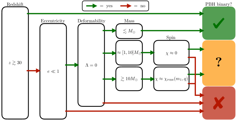
Figure 1: Schematic flowchart to systematically rule out or potentially assess the primordial nature of a binary merger based on measurements of the redshift $z$, eccentricity $e$, tidal deformability $\Lambda$, component masses $m$, and dimensionless spins $\chi$. Each arrow indicates if the condition in the box is met (green) or violated (red). The various marks indicate: ✓) likely to be a PBH binary; ✗) cannot to be a PBH binary; ?) may be a PBH binary.

I Introduction

The collapse of very large inhomogeneities during the radiation-dominated era could produce primordial black holes (PBHs) Zel’dovich and Novikov (1967); Hawking (1974); Chapline (1975); Carr (1975) across a wide mass range Ivanov et al. (1994); Garcia-Bellido et al. (1996); Ivanov (1998); Blinnikov et al. (2016). Despite several observational constraints on these objects (see Carr et al. (2020) for a recent review), in certain mass ranges PBHs could comprise the entirety of the dark matter, and could seed supermassive black holes (BHs) at high redshift Volonteri (2010); Clesse and García-Bellido (2015); Serpico et al. (2020). Furthermore, PBHs could contribute to at least a fraction of the BH merger events detected by LIGO-Virgo Abbott et al. (2019a, 2021a, 2021b) so far Bird et al. (2016); Sasaki et al. (2016); Eroshenko (2018); Wang et al. (2018); Ali-Haïmoud et al. (2017); Chen and Huang (2018); Raidal et al. (2019); Liu et al. (2019a); Hütsi et al. (2019); Vaskonen and Veermäe (2020); Gow et al. (2020); Wu (2020); De Luca et al. (2020a); Hall et al. (2020); Wong et al. (2021); Hütsi et al. (2021); Kritos et al. (2021); De Luca et al. (2021a); Deng (2021); Kimura et al. (2021); Franciolini et al. (2021); Bavera et al. (2021); Liu et al. (2021), and to those that will be detected by future gravitational-wave (GW) instruments De Luca et al. (2021a, b); Pujolas et al. (2021): see Refs. Abbott et al. (2021b, c) for the most recent LIGO-Virgo-KAGRA (LVK) Collaboration catalog and population studies, and Refs. Sasaki et al. (2018); Green and Kavanagh (2021); Franciolini (2021) for reviews on PBHs as GW sources.

“Special” events such as GW190425 (with a total mass that exceeds that of known galactic neutron star binaries) and the mass-gap events (such as GW190814 Clesse and Garcia-Bellido (2020), GW190521 De Luca et al. (2021c) and GW190426_190642) may have a PBH origin. Also, a subpopulation of PBHs may be competitive with certain astrophysical population models at explaining a fraction of events detected thus far by the LVK Collaboration Franciolini et al. (2021). However, astrophysical uncertainties make it hard to draw definite conclusions at a population level, and confidently claiming the primordial origin of an individual BH merger is much more challenging. Indeed, an important problem in the “PBHs as GW sources” program is to disentangle a PBH candidate from the astrophysical foreground, thus discriminating between the primordial or astrophysical origin of a given binary. Attempts have been made for single-event detections using Bayesian model selection based on astrophysically or primordial-motivated different priors Bhagwat et al. (2021), whereas catalog analyses could use the peculiar mass-spin-redshift distributions predicted for PBH binaries Raidal et al. (2019); De Luca et al. (2020a) or perform population studies Hall et al. (2020); Wong et al. (2021); Hütsi et al. (2021); De Luca et al. (2021a); Franciolini et al. (2021). Given current measurement accuracy, the relatively modest number of GW events, and the uncertainties in both PBH and astrophysical models, none of the aforementioned strategies is currently able to give irrefutable evidence for or against the PBH scenario Franciolini et al. (2021).

This state of affairs is expected to improve greatly in the era of next-generation detectors, such as the third-generation (3G) ground-based interferometers Cosmic Explorer (CE) Reitze et al. (2019) and Einstein Telescope (ET) Hild et al. (2011), and the future space mission LISA Amaro-Seoane et al. (2017). In particular, 3G detection rates will be orders of magnitude larger than current ones Baibhav et al. (2019); Maggiore et al. (2020); Kalogera et al. (2021), and much more accurate measurements will be possible for “golden” events with high signal-to-noise ratio (SNR).

The main goal of this paper is to present a systematic discussion of the various discriminators that would allow us to either rule out or confidently claim the primordial origin of a GW event by measuring different key binary parameters: the redshift, masses, spins, eccentricity, and tidal deformability (see Sec. II). A systematic strategy to use these discriminators is summarized in the flowchart of Fig. 1, based on the predictions of the standard PBH scenario summarized in Sec. II (where we also discuss some caveats). In Sec. III we estimate the measurement errors on the PBH discriminators needed to apply this flowchart, and we quantify their constraining power for current and future detectors. In Sec. IV we apply the strategy to the GWTC-3 event catalog. We conclude in Sec. V with a summary of our findings and a discussion of future research directions.

We will focus on binaries with individual component masses up to around ${\cal O}(10^{2})M_{\odot}$, which comprise all of the events currently observed by LVK. We do not attempt to assess the primordial nature of more massive BHs, up to the supermassive range potentially detectable by LISA. Accretion throughout the cosmological evolution prior to the reionization epoch is still poorly modelled for those PBHs, and the predictions used in this paper (following Refs. De Luca et al. (2020b, a)) have not been properly extended including feedback effects: see the discussion in Ref. Ricotti et al. (2008). Therefore we leave this effort for future work. Throughout this paper we adopt geometrical units ($G=c=1$).

II Key predictions for PBHs

In this section, we review the main properties of PBH binaries, whose characteristic features will be used in the rest of the paper to address the question: how can we rule out or confirm the primordial origin of a merger signal? We highlight that throughout this work we will consider the “standard” PBH formation scenario, in which PBHs are formed out of large density fluctuations in the radiation dominated Universe Sasaki et al. (2018). We will comment later on about other possible PBH scenarios, and whether they may lead to different predictions.

To clarify our notation, we consider binaries with masses $m_{1}$ and $m_{2}$, mass ratio $q=m_{2}/m_{1}\leq 1$, total mass $M=m_{1}+m_{2}$, and dimensionless spins $\chi_{i}=J_{i}/m_{i}^{2}$ (with $0\leq\chi_{j}\leq 1$), located at redshift $z$. Additionally, an important parameter measurable through GW observations is the effective spin

$$\chi_{\text{\tiny eff}}\equiv\frac{\chi_{1}\cos{\alpha_{1}}+q\chi_{2}\cos{\alpha_{2}}}{1+q},$$ (1)

which is a function of the mass ratio $q$, of both BH spin magnitudes $\chi_{j}$ ($j=1,2$), and of their orientation with respect to the orbital angular momentum, parametrized by the tilt angles $\alpha_{j}$.

II.1 PBH binary formation vs redshift

In the standard formation scenario, PBHs are generated from the collapse of large overdensities in the primordial Universe Ivanov et al. (1994); Garcia-Bellido et al. (1996); Ivanov (1998); Blinnikov et al. (2016) (see Green and Kavanagh (2021) for a recent review). As the PBH mass is related to the size of the cosmological horizon at the time of collapse, the formation of a PBH of mass $m_{\text{\tiny{PBH}}}$ takes place deep in the radiation-dominated era, at a typical redshift Sasaki et al. (2018)

$$z_{\text{\tiny i}}\approx 2\times 10^{11}\left({m_{\text{\tiny{PBH}}}}\over{M_{\odot}}\right)^{-1/2}.$$ (2)

At that epoch, the standard scenario predicts that PBH locations in space are described by a Poisson distribution (Ali-Haïmoud, 2018; Desjacques and Riotto, 2018; Ballesteros et al., 2018; Moradinezhad Dizgah et al., 2019; De Luca et al., 2020c). In simple terms, this means that the number of PBHs in a given volume $V$ is described by a Poisson distribution with mean $\lambda=n_{\text{\tiny PBH}}\times V$, where $n_{\text{\tiny PBH}}$ is the average number density of PBHs in the Universe. This initial condition is used to compute the properties of the population of PBH binaries formed at high redshift and contributing to the PBH merger rate.

It is important to stress that the merger rate of PBHs is dominated by binaries formed in the early Universe via gravitational decoupling from the Hubble flow before the matter-radiation equality Nakamura et al. (1997); Ioka et al. (1998). Another binary formation mechanism is possible, i.e., the formation of binaries taking place in present-day halos through gravitational capture. This second possibility was previously considered in the literature, see for example Refs. Bird et al. (2016); Cholis et al. (2016), but it was later on shown to produce a largely subdominant contribution to the overall merger rate Ali-Haïmoud et al. (2017); Raidal et al. (2017); Vaskonen and Veermäe (2020); De Luca et al. (2020d). We will, therefore, only consider the former mechanism throughout this paper. As a consequence, in contrast to the astrophysical channels, primordial binary BHs (BBHs) have a merger rate density that monotonically increases with redshift as (Ali-Haïmoud et al., 2017; Raidal et al., 2019; De Luca et al., 2020a)

$$R_{\text{\tiny PBH}}(z)\propto\left(\frac{t(z)}{t(z=0)}\right)^{-34/37},$$ (3)

extending up to redshifts $z\gtrsim{\cal O}(10^{3})$. Notice that the evolution of the merger rate with time shown in Eq. (3) is entirely determined by the binary formation mechanism (i.e. how pairs of PBHs decouple from the Hubble flow) before the matter-radiation equality era. Eq. (3) is, therefore, a robust prediction of the PBH model in the standard formation scenario.

On the contrary, astrophysical-origin mergers should not occur at $z\gtrsim 30$. The redshift corresponding to the epoch of first star formation is poorly known: theoretical calculations and cosmological simulations suggest this to fall below $z\sim 40$ Schneider et al. (2000, 2002, 2003); Bromm (2006); de Souza et al. (2011); Koushiappas and Loeb (2017); Mocz et al. (2020); Liu and Bromm (2020a) (but see Refs. Trenti and Stiavelli (2009) and Tornatore et al. (2007), where Pop III star formation was suggested to start at higher or lower redshift). The time delay between Pop III star formation and BBH mergers was studied using population synthesis models, and found to be around $\mathcal{O}(10)~{}\rm Myr$ Kinugawa et al. (2014, 2016); Hartwig et al. (2016); Belczynski et al. (2017); Inayoshi et al. (2017); Liu and Bromm (2020b, a); Kinugawa et al. (2020); Tanikawa et al. (2021); Singh et al. (2021). This means that we can conservatively assume BBHs from Pop III remnants to merge below $z\approx 30$, and consider merger redshifts $z\gtrsim 30$ to be smoking guns for primordial binaries Koushiappas and Loeb (2017); De Luca et al. (2021a); Ng et al. (2021).

II.2 PBH masses and spins

The distribution of PBH masses $m_{\text{\tiny{PBH}}}$ is determined by the characteristic size and statistical properties of the density perturbations, corresponding to curvature perturbations generated during the inflationary epoch. As $m_{\text{\tiny{PBH}}}$ is related to the mass contained in the cosmological horizon at the time of collapse, a much wider range of masses is accessible compared to astrophysical BHs Sasaki et al. (2018). In particular, PBHs can have subsolar masses, which are unexpected from standard stellar evolution, and they can also populate the astrophysical mass gaps Clesse and Garcia-Bellido (2020); De Luca et al. (2021c).

Given an accurate mass measurement, we can discriminate among three cases:

• $m_{i}\lesssim M_{\odot}$: subsolar compact objects could be PBHs, white dwarfs, brown dwarfs, or exotic compact objects Cardoso and Pani (2019), e.g. boson stars Guo et al. (2019). Distinguishing PBHs from other compact objects requires taking into account tidal disruption and tidal deformability measurements (see Sec. II.4 below). As we will see, less compact objects like brown and white dwarfs are tidally disrupted well before the contact frequency, so detecting the merger of a subsolar compact object would imply new physics, regardless of the nature of the object Barsanti et al. (2021).

• $1\lesssim m_{i}/M_{\odot}\lesssim 3$: PBHs in this mass range can be confused with neutron stars (NSs). Once again, tidal deformability measurement can in principle be used to break the degeneracy. Additionally, solar-mass BHs can form out of NS transmutation in certain particle-dark-matter scenarios Bramante et al. (2018); Takhistov et al. (2021); Dasgupta et al. (2021); Giffin et al. (2021). In the upper half of this mass range ($2\lesssim m_{i}/M_{\odot}\lesssim 3$), the component BHs in the binary may form out of previous NS-NS mergers and then pair again to produce a light binary Fasano et al. (2020). In this case, however, the second-generation BH formed as a result of the NS-NS merger is expected to be spinning Hofmann et al. (2016). This is in contrast with the prediction for the PBH scenario in this mass range, as we shall see in the following.

• $m_{i}>3M_{\odot}$: PBHs in this mass range must be distinguished from stellar-origin BHs by other means.

Obviously, the boundaries between the mass ranges discussed above should be understood as approximate, and taken with a grain of salt.

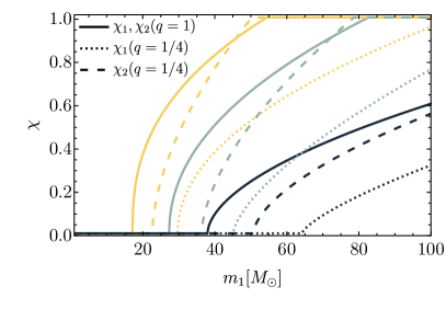
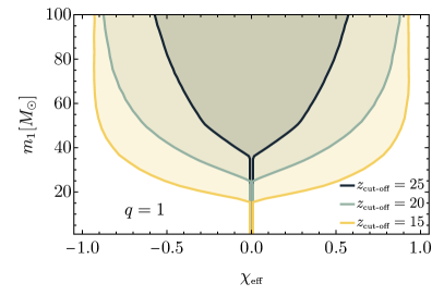
Figure 2: Left: Predicted primary ($\chi_{1}$) and secondary ($\chi_{2}$) spins as a function of primary mass and mass ratio for various values of $z_{\text{\tiny\rm cut-off}}$ (indicated by the same colors as in the right panel). The plot highlights that for unequal mass binaries, the PBH accretion model predicts the secondary spin component $\chi_{2}$ to be larger than the primary component $\chi_{1}$. Right: Predicted distribution of $\chi_{\text{\tiny\rm eff}}$ as a function of $m_{1}=m_{2}$ for three selected values of $z_{\text{\tiny\rm cut-off}}$.

Another important property of a PBH is its spin $\chi$. Since extreme Gaussian perturbations tend to have nearly-spherical shape Bardeen et al. (1986) and the collapse takes place in a radiation-dominated Universe, the initial dimensionless Kerr parameter $\chi\equiv J/M^{2}$ (where $J$ and $M$ are the angular momentum and mass of the BH) is expected to be below the percent level De Luca et al. (2019); Mirbabayi et al. (2020). However, a nonvanishing spin can be acquired by PBHs forming binaries through an efficient phase of accretion De Luca et al. (2020a, b) prior to the reionization epoch.

Accretion during the cosmic evolution was shown to be effective only for PBHs with masses above $m_{\text{\tiny{PBH}}}\gtrsim{\cal O}(10)M_{\odot}$. Therefore, the PBH model predicts binaries with negligible spins in the “light” portion of the observable mass range of current ground-based detectors. At larger masses, a defining characteristic of the PBH model is the expected correlation between large binary total masses and large values of the spins of their PBH constituents, induced by accretion effects. In addition, the spin directions of PBHs in binaries are, at least following the modeling of accretion described in Ref. De Luca et al. (2020a), independent and randomly distributed on the sphere. We will consider this scenario in the remainder of the paper, but we warn the reader that details of the accretion dynamics are still rather uncertain, and exceptions to the prediction of random spin orientations are possible. Overall, PBH accretion is still affected by large uncertainties, in particular coming from the impact of feedback effects Ricotti (2007); Ali-Haïmoud et al. (2017), structure formation Hasinger (2020); Hütsi et al. (2019), and early X-ray pre-heating (e.g. (Oh and Haiman, 2003)). Therefore, in recent years, an additional hyperparameter (the cut-off redshift $z_{\text{\tiny cut-off}}\in[10,30]$) was introduced to account for accretion model uncertainties De Luca et al. (2020b). For each value of $z_{\text{\tiny cut-off}}$ there is a one-to-one correspondence between the initial and final masses, which can be computed according to the accretion model described in detail in Refs. (Ricotti, 2007; Ricotti et al., 2008; De Luca et al., 2020a, b, e). We highlight, for clarity, that a lower cut-off is associated to stronger accretion and vice-versa. Values above $z_{\text{\tiny cut-off}}\simeq 30$ effectively correspond to negligible accretion in the mass range of interest for LVK observations. For detections at high redshift $z>z_{\text{\tiny cut-off}}$ (as those potentially achievable with 3G detectors), one expects a characteristic $z-\chi$ correlation.

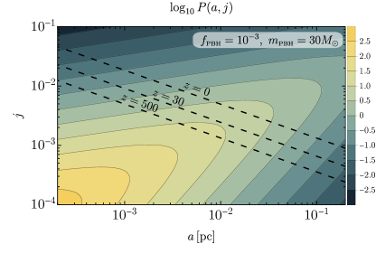
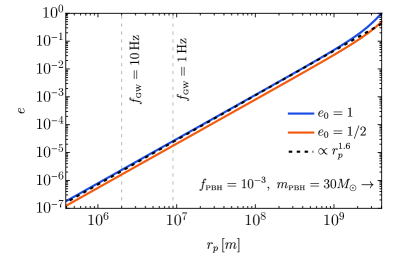
Figure 3: Left: Probability distribution of semimajor axis $a$ and rescaled angular momentum $j$ for PBH binaries of a population described by $f_{\text{\tiny\rm PBH}}=10^{-3}$ and $m_{\text{\tiny\rm PBH}}=30M_{\odot}$. The black dashed lines indicate the combination of parameters giving a merger time equal to the age of the Universe at various redshift $z=[0,\,30,\,500]$. Right: Eccentricity evolution for a characteristic binary merging at low redshift ($z\approx 0$) formed from a PBH population with $f_{\text{\tiny\rm PBH}}=10^{-3}$ and $m_{\text{\tiny\rm PBH}}=30M_{\odot}$, whose initial pericenter distance $r_{p}$ at the binary formation epoch is indicated by the arrow. As an indication, we also show the power-law scaling relating the eccentricity $e$ to $r_{p}$.

It is possible to derive an analytical fit of the relation between the masses and spins predicted at low redshift (that is, $z\lesssim z_{\text{\tiny cut-off}}$) as a function of $z_{\text{\tiny cut-off}}\supset[10,30]$. This fit describes the magnitude of both individual spins $\chi_{i}$ (where $i=1,2$) in PBH binaries as a function of the primary mass and mass ratio in the ranges $m_{1}\lesssim 10^{2}M_{\odot}$ and $q\gtrsim 0.1$, respectively. The fit was derived using the results of the numerical integration of the equations describing accretion onto PBH in binaries as modelled in Refs. De Luca et al. (2020b, a). It could be useful when performing Bayesian parameter estimations assuming PBH motivated priors, or for searches in GW catalogs for a PBH-motivated mass-spin relation. It can be written parametrically as

$$\chi_{i}(m_{1},q,z_{\text{\tiny cut-off}}) \approx 10^{-2}+{\rm Min}\left[0.988,10^{f^{b}_{i}}\left(\frac{m_{1}}{M_{\odot}}-{f^{a}_{i}}\right)^{f^{c}_{i}}\right.$$

$$\times\left.\Theta\left(\frac{m_{1}}{M_{\odot}}-{f^{a}_{i}}\right)\right],$$ (4)

where $\Theta$ is the Heaviside theta function, and each coefficient $f^{a,b,c}_{i}$ depends on both $z_{\text{\tiny cut-off}}$ and $q$. Those functions are expanded as a polynomial series of the form

$$f^{\alpha}_{i}(z_{\text{\tiny cut-off}},q) =\alpha_{i}^{0}+\sum_{j=1}^{3}\alpha_{i}^{z,j}\left(\frac{z_{\text{\tiny cut-off}}}{10}\right)^{j}+\sum_{j=1}^{3}\alpha_{i}^{q,j}q^{j}$$

$$+\sum_{j,k=1}^{2}\alpha_{i}^{j,k}\left(\frac{z_{\text{\tiny cut-off}}}{10}\right)^{j}q^{k},$$ (5)

with $\alpha=[a,b,c]$. Note that the terms in the polynomial expansion involving the cut-off redshift are renormalized as a function of $(z_{\text{\tiny cut-off}}/10)$ for numerical convenience. The fit percentile error is below $10\%$ in the vast majority ($>98\%$) of the parameter space, while it degrades to around $30\%$ close to the boundaries of the $(m_{1},\,q,\,z_{\text{\tiny cut-off}})$ space. The coefficients in the analytical relation are reported in Appendix A. In Fig. 2, we show the expected distribution of $\chi_{\text{\tiny eff}}$ produced using Eq. (II.2) and by averaging over the spin angles, as a function of PBH masses in binaries for various choices of $z_{\text{\tiny cut-off}}$.

After this summary, we would like to stress once more that these predictions assume the standard PBH scenario, where PBHs are formed through the collapse of large overdensities during the radiation phase. There are other possible scenarios, such as formation from assembly of matterlike objects (particles, Q-balls, oscillons, etc.), domain walls and heavy quarks of a confining gauge theory, which may lead to different predictions for the PBH spin at formation Harada et al. (2017); Flores and Kusenko (2021); Dvali et al. (2021); Eroshenko (2021). For instance, during an early matter-dominated phase, possibly following the end of inflation and preceding the reheating phase, PBHs may be formed in a pressureless environment and develop initial large, and possibly maximal, spins Harada et al. (2017); De Luca et al. (2021d). Such scenarios would require dedicated analyses, but we remark that the impact of accretion (when relevant) onto the mass-spin correlation and the properties of the remaining observables (i.e. redshift distribution, eccentricity and masses) remain consistent with the standard scenario.

II.3 PBH eccentricity

Another key prediction of the primordial model involves the eccentricity $e$ of PBH binaries. While formed with large eccentricity at high redshift, PBH binaries then have enough time to circularize before the GW signal can enter the observation band of current and future detectors. In this section we quantify this statement.

II.3.1 Eccentricity distribution at formation

We start by defining the mean PBH separation at matter-radiation equality as

$$\bar{x}\equiv\left(\frac{3m_{\text{\tiny{PBH}}}}{4\pi f_{\text{\tiny{PBH}}}\,\rho_{\mathrm{eq}}}\right)^{1/3},$$ (6)

where $\rho_{\text{\tiny eq}}$ is the average energy density at matter-radiation equality and $f_{\text{\tiny{PBH}}}$ is the fraction of dark matter in PBHs. As predicted by the standard formation scenario in the absence of primordial nongaussianities, PBHs follow a Poisson spatial distribution at formation. One can show that the differential probability distribution of the rescaled angular momentum $j\equiv\sqrt{1-e^{2}}$ reads Ali-Haïmoud et al. (2017); Kavanagh et al. (2018); Liu et al. (2019b)

$$jP(j) =\frac{y(j)^{2}}{\left(1+y(j)^{2}\right)^{3/2}},$$

$$y(j) \equiv\frac{j}{0.5(1+\sigma_{\text{\tiny eq}}^{2}/f_{\text{\tiny{PBH}}}^{2})^{1/2}\left({x}/{\bar{x}}\right)^{3}},$$ (7)

where $\sigma_{\text{\tiny eq}}\approx 0.005$ indicates the variance of the Gaussian large-scale density perturbations at matter-radiation equality. This distribution is the result of both the surrounding PBHs and matter perturbations producing a torque on the PBH binary system during its formation. Finally, the distribution describing both $j$ and the semimajor axis $a$ can be written as

$$P(a,j)=\frac{3}{4a^{1/4}}\left(\frac{f_{\text{\tiny PBH}}}{\alpha\bar{x}}\right)^{3/4}P(j)\exp\left[-\left(\frac{x(a)}{\bar{x}}\right)^{3}\right],$$ (8)

where

$$x(a)\equiv\left(\frac{3\,a\,m_{\text{\tiny PBH}}}{4\pi\,\alpha\,\rho_{\text{\tiny eq}}}\right)^{1/4}$$ (9)

and $\alpha\simeq 0.1$ Ali-Haïmoud et al. (2017). This distribution is shown in Fig. 3.

We are interested in finding the probability distribution of the angular momentum of binaries constrained by the requirement of merging at redshift $z_{\text{\tiny merge}}$ (or time $t_{\text{\tiny merge}}$). We compute, therefore, the merger time $t_{\text{\tiny merge}}$ of primordial binaries using Peter’s formula Peters and Mathews (1963a); Peters (1964) (see also Mandel (2021)). For a binary of equal masses $m_{1}=m_{2}=m_{\text{\tiny{PBH}}}$, initial eccentricity $e_{0}$ and semimajor axis $a_{0}$, and in the limit of large initial eccentricity, one finds

$$\tau=\frac{3}{170}\frac{a_{0}^{4}}{m_{\text{\tiny{PBH}}}^{3}}\left(1-e_{0}^{2}\right)^{7/2}.$$ (10)

In the left panel of Fig. 3 we also show by dashed black lines the set of parameters $(a,j)$ giving rise to a merger at redshift $z=[0,30,100]$. Note that while the value of $f_{\text{\tiny{PBH}}}$ has a major impact on the overall probability of forming a PBH binary (and the consequent overall merger rate), it affects only slightly the shape of the probability density function for the orbital parameters.

II.3.2 Eccentricity evolution

The predictions for the initial binary parameters of PBHs should be used to forecast the final eccentricity when the GW enters the observability band of current ground-based detectors. As PBH binaries form at very high redshift, observable signals are coming from binaries which are initially wide enough so that the merger time is close to the current age of the Universe. As GW emission circularizes the orbit, one expects PBH binaries to lose any relevant eccentricity before detection.

Let us show this explicitly. Rearranging the equations describing the orbital evolution under the effect of GW emission, and defining the pericenter distance

$$r_{p}\equiv a(1-e),$$ (11)

one obtains Maggiore (2007)

$$r_{p}\frac{{\rm d}e}{{\rm d}r_{p}}=e(1+e)\frac{304+121e^{2}}{192-112e+168e^{2}+47e^{3}},$$ (12)

which, in the limit of quasicircular orbits $e\ll 1$, simplifies to

$$\frac{{\rm dln}e}{{\rm dln}r_{p}}\simeq\frac{304}{192}\simeq 1.6.$$ (13)

We show the evolution of the eccentricity as a function of $e_{0}$ in Fig. 3 (right panel). For a characteristic PBH binary formed by a narrow PBH population with $f_{\text{\tiny{PBH}}}=10^{-3}$ and $m_{\text{\tiny{PBH}}}=30M_{\odot}$ and expected to merge at $z\simeq 0$, one finds an initial binary pericenter distance of the order of $r_{p}\simeq 4\times 10^{9}\,{\rm m}$. In the figure we also indicate the eccentricity at which the binary would approximately enter the ET and LVK observable band with a frequency of $1$ and $10$ Hz, respectively. Those frequencies corresponds to roughly $r_{p}\simeq 22R_{\text{\tiny Sch}}\simeq 2\times 10^{6}{\rm m}$ ($r_{p}\simeq 102R_{\text{\tiny Sch}}\simeq 9\times 10^{6}{\rm m}$) for $m_{\text{\tiny{PBH}}}=30M_{\odot}$, where the eccentricity of the orbit has already been reduced to a value below $e\approx 10^{-5}$.

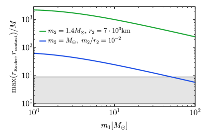
Figure 4: Left: Maximum between the Roche radius and the contact radius, $r_{2}+2m_{1}$, normalized by the total binary mass $M$, as a function of the primary mass $m_{1}$ for two representative examples of secondary object: a white dwarf (blue) and a solar-mass mini boson star (green). The horizontal gray band brackets the ISCO of a spinning BH ($1<r_{\text{\tiny\rm ISCO}}/M<9$). This plot indicates that compact objects such as white dwarfs and mini boson stars are usually disrupted before reaching the ISCO. For both chosen examples, ${\rm max}(r_{\text{\tiny\rm Roche}},r_{\text{\tiny\rm contact}})=r_{\text{\tiny\rm Roche}}$. Right: Focusing on NS-BH binaries, the plot shows the minimum mass ratio above which the NSs get disrupted depending on the NS compactness ${\cal C}$ and BH spin $\chi$. We use the disruption criterion of Ref. Pannarale et al. (2015), which is based on numerical NS-BH merger simulations.

We can use the GW frequency evolution as a function of the eccentricity to estimate the eccentricity of the binary at the smaller frequencies accessible to 3G detectors. Since (see e.g. Peters and Mathews (1963a); Peters (1964); Kowalska et al. (2011))

$$f_{\text{\tiny GW}}(e)=\frac{2}{P_{0}}\frac{(1-e^{2})^{3/2}}{e^{18/19}}\left[1+\frac{121}{304}e^{2}\right]^{-1305/2299}c_{0}^{3/2},$$ (14)

where $c_{0}=[e_{0}^{12/19}(1+{121}e_{0}^{2}/{304})^{1305/2299}]/(1-e_{0}^{2})$ and $P_{0}$ is the initial orbital period, we can infer that in the limit of small eccentricity

$$e\propto f_{\text{\tiny GW}}^{-19/18}.$$ (15)

Since detectors such as ET are potentially sensitive down to frequencies $\approx 1{\rm Hz}$, the above scaling shows that the eccentricity of the binary when it enters the 3G band is only a factor ${\cal O}(10)$ bigger than when it enters the LIGO band, and it is still negligible for PBH binaries.

So far we have considered mergers happening at low redshift $z\lesssim 1$. In case of high-redshift mergers ($z\gtrsim 30$) predicted by the primordial scenario, the initial PBH binary semimajor axis is reduced by only a factor ${\cal O}$(2), as shown in Fig. 3. This small change is due to the large sensitivity of the merger time to the initial semimajor axis: $\tau\propto a_{0}^{4}$, see Eq. (10). Therefore, when the binary enters the detectable frequency band of GW experiments, it is expected to have already circularized its orbit to an undetectable level. This property allows us to distinguish primordial binaries from binaries produced by astrophysical dynamical formation channels, which may retain significant eccentricities (see e.g. Refs. Samsing et al. (2014); Nishizawa et al. (2016); Breivik et al. (2016); Nishizawa et al. (2017); Zevin et al. (2021)).

Let us recall one more time that our predictions are based on the assumption that PBH mergers are dominated by the binaries formed in the early Universe. If late-time Universe binaries contribute substantially to the observed events, the PBH binary eccentricity may be larger, and comparable to expectations from the astrophysical dynamical formation scenarios. This situation may be realized with strong PBH clustering suppressing the early-Universe binary merger rate, while enhancing the late-time Universe contribution Jedamzik (2020); Vaskonen and Veermäe (2020); Trashorras et al. (2021); De Luca et al. (2020d). However, we stress that this scenario would require a large value of the PBH abundance ($f_{\text{\tiny{PBH}}}\simeq 1$), which is in contrast with current PBH constraints in the LVK mass range Carr et al. (2020).

II.4 Tidal disruption and tidal deformability

While PBHs below a few solar masses can be easily distinguished from a population of (heavier) stellar-origin BHs, they might be confused with other compact objects. For example, in standard astrophysical scenarios, white dwarfs and NSs are formed with masses above $\approx 0.2M_{\odot}$ Kilic et al. (2007) and $\approx 1M_{\odot}$ Strobel et al. (1999); Lattimer (2012); Silva et al. (2016); Suwa et al. (2018), respectively.

A relevant discriminator in this case is provided by the Roche radius, ${r_{\text{\tiny Roche}}}$, below which the secondary object in a binary system gets tidally disrupted, if it is not a BH. The Roche radius is approximately

$${r_{\text{\tiny Roche}}}\sim 1.26\,r_{2}q^{-1/3}\,,$$ (16)

where $r_{2}$ is the radius of the secondary object. If ${r_{\text{\tiny Roche}}}>r_{\text{\tiny ISCO}}\sim{\cal O}(M)$, the binary is tidally disrupted before merger, thus effectively cutting off the GW signal at the GW frequency corresponding to $r_{\text{\tiny Roche}}$. Another relevant quantity to check is the contact radius which, assuming the primary is a BH, can be estimated as

$$r_{\text{\tiny contact}}\sim 2m_{1}+r_{2}\,.$$ (17)

If $r_{\text{\tiny contact}}>r_{\text{\tiny ISCO}}$ the contact frequency of the objects is lower than the ISCO frequency, and the point-particle approximation breaks down.

The left panel of Fig. 4 shows that, for a typical white dwarf, ${\rm max}(r_{\text{\tiny Roche}},r_{\text{\tiny contact}})=r_{\text{\tiny Roche}}$ is larger than the ISCO. Therefore, the star is tidally disrupted well before the GW signal reaches the ISCO frequency. Less compact objects, such as brown dwarfs, are disrupted at even larger radii (smaller orbital frequencies). Therefore, if $m_{2}<M_{\odot}$ (thus excluding NSs) the maximum frequency of the coalescence can be used to detect a tidal disruption event and discriminate whether the secondary is a BH or a less compact star. When the secondary is a NS, the possible outcomes are more complicated. We may still have nondisruptive mergers if the NS compactness (i.e. the ratio between the mass and the size of the NS, ${\cal C}\equiv m_{\text{\tiny NS}}/r_{\text{\tiny NS}}$) is large enough, or if the ratio between the secondary (NS) mass and the primary (BH) mass is sufficiently small: see the right panel of Fig. 4, based on the criterion in Ref. Pannarale et al. (2015). In this case, the absence of tidal disruption may not be used as a discriminator for the (primordial) BH nature of the secondary object.

Exotic compact objects Cardoso and Pani (2019) (e.g. boson stars Liebling and Palenzuela (2012)) would provide another possible explanation for a (sub)solar compact object. The compactness of a boson star depends strongly on its mass and on the scalar self interactions Cardoso et al. (2017). For the vanilla “mini” boson star model without self-interactions Ruffini and Bonazzola (1969), the compactness is $m_{2}/r_{2}={\cal O}(0.01)$ near the maximum mass. The left panel of Fig. 4 shows that also solar-mass mini boson stars would be tidally disrupted before the ISCO. In the presence of strong scalar self-interactions, boson stars can be as compact as a NS Colpi et al. (1986); Cardoso et al. (2017), so in that case the tidal disruption is not a clear-cut discriminator.

Another key discriminator between PBHs and (sub)solar horizonless objects is the absence, in the former case, of tidal deformability contributions to the gravitational waveform. The tidal Love numbers are identically zero for a BH (see Refs. Binnington and Poisson (2009); Damour and Nagar (2009); Damour and Lecian (2009); Pani et al. (2015a, b); Gürlebeck (2015); Porto (2016); Le Tiec and Casals (2021); Chia (2020); Le Tiec et al. (2021); Hui et al. (2021); Charalambous et al. (2021a, b); Pereñiguez and Cardoso (2021) for literature on this topic) , whereas they are generically nonzero and model-dependent for any other compact object Cardoso et al. (2017). The tidal Love numbers enter the GW phase in Eq. (28) starting at 5 post-Newtonian (PN) order. We write

$$\Delta\Psi^{\text{\tiny tidal}}_{\text{\tiny 6PN}}=\Lambda v^{5}+\delta\Lambda v^{6}+{\cal O}(v^{7})\,,$$ (18)

where $v=(\pi Mf)^{1/3}$ is the PN orbital velocity parameter, and the $5$PN and $6$PN terms are given by Flanagan and Hinderer (2008); Vines et al. (2011)

$$\Lambda =\left(264-\frac{288}{\eta_{1}}\right)\frac{\lambda_{2}^{(1)}}{M^{5}}+(1\leftrightarrow 2)\,,$$

$$\delta\Lambda =\left(\frac{4595}{28}-\frac{15895}{28\eta_{1}}+\frac{5715\eta_{1}}{14}-\frac{325\eta_{1}^{2}}{7}\right)\frac{\lambda_{2}^{(1)}}{M^{5}}+(1\leftrightarrow 2)\,,$$ (19)

in terms of the dominant (i.e., electric-type, quadrupolar) tidal Love number, $\lambda_{2}^{(i)}=2m_{i}^{5}k_{2}^{(i)}/3$, of the $i$-th body. In the Newtonian approximation, the tidal Love number of an object is (see e.g. Poisson and Will (1953))

$$k_{2}^{(i)}\sim{\cal O}(0.01-0.1)\left(\frac{r_{i}}{m_{i}}\right)^{5}\,,$$ (20)

where the precise value of the dimensionless prefactor depends on the nature of the object (for instance, on the equation of state in the case of a NS). Thus, less compact objects have the larger tidal deformability, and hence can be more easily discriminated from a BH.

Overall, any measurement of a nonzero tidal deformability in an object above a few solar masses would automatically imply that either the object is not a BH, or that the BH is surrounded by matter fields, in which case the total tidal Love number of the dressed BH is nonzero Cardoso and Duque (2020); De Luca and Pani (2021).

Finally, a further discriminator would be the waveform corrections due to tidal heating terms in the case of BHs. This correction is due to dissipation at the event horizon Alvi (2001) and is negligible for other compact objects Cardoso and Pani (2019); Maselli et al. (2018). However, the contribution of the tidal heating is typically small. Unless the object is extremely compact so that $k_{2}\sim 0$, tidal heating is subdominant with respect to the tidal deformability correction presented above.

III Measurement accuracy for key PBH binary discriminants

In this section we quantify the measurability of the PBH discriminators presented above, following the flowchart of Fig. 1. The statistical errors are computed using a Fisher information matrix approach, which provides an accurate estimate of the statistical errors in the high-SNR limit with Gaussian noise and in the absence of systematic biases in the waveform parameters Vallisneri (2008). Our methodology is standard, and reviewed in Appendix B for completeness.

We will present results for the planned future stage of the LIGO experiment (Ad. LIGO), the 3G detector ET (in its ET-D configuration Hild et al. (2011)) and LISA Robson et al. (2019). We do not explicitly report the analysis for the CE detector, because the CE noise power spectral density is qualitatively similar to ET. The noise power spectral densities used in our analysis are listed in Appendix B.2.1.

As we discussed in the introduction, we will focus on binary mergers with individual component masses below ${\cal O}(10^{2})M_{\odot}$. We leave the analysis of more massive events, up to the supermassive range of interest for LISA, for future work.

Figure 5: Relative percentage errors on redshift measurement for an optimally oriented source located at redshift $z$, detected with ET. The various colors correspond to different choices of total mass $M$.

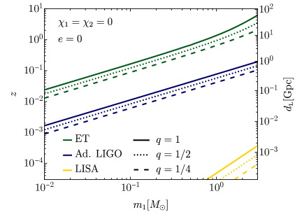
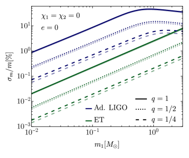
Figure 6: Left: Horizon redshift as a function of SNR for subsolar-mass mergers assuming noneccentric, spinless and optimally oriented binaries for different values of the mass ratio. In this mass range, due to the different range of frequencies probed by space-based detectors, LISA will have very limited reach and its horizon can only be seen in the bottom right corner. Right: Measurement errors of the binary’s primary and secondary masses in the subsolar range. The binaries are assumed to be located at the horizon redshift of Ad. LIGO following the same assumptions as in the left panel. We assumed the same distance for ET to highlight the improved precision of the 3G detector. The dashed and dotted lines indicate smaller values of the mass ratio. In the cases $q\neq 1$, the percentile uncertainties on the primary (secondary) mass is indicated with a darker (lighter) color, which corresponds to the higher (lower) line.

III.1 Redshift measurement accuracy

Next-generation interferometers such as CE and ET will be able to search for PBH mergers at redshift $z\gtrsim 30$, where mergers of astrophysical origin should not occur Koushiappas and Loeb (2017); De Luca et al. (2021a). However, redshift measurements for such distant cosmological sources are typically inaccurate and prior-dependent Ng et al. (2021). In Fig. 5, we show the measurement errors estimated using the Fisher matrix analysis for distant events with large source redshift and four selected values of the total mass. The measurement accuracy we obtain is consistent with the errors computed using a full Bayesian parameter estimation in Ref. Ng et al. (2021), but the Fisher formalism does not allow us to reproduce the bias towards smaller redshift observed in their results. This systematic bias is due to a combination of the assumed prior on the source redshift, and the asymmetric dependence of the errors on binary inclination angles  Ng et al. (2021), and it is partly responsible for the difficulty in confidently assessing the high-redshift ($z\gtrsim 30$) nature of distant binaries. Note also that we do not report results for total masses $M\gtrsim 60M_{\odot}$ because, in that case, the SNR is dominated by the merger-ringdown portion of the GW signal, which we are not including in our simple estimates.

LISA will also be able to observe events with $z\gtrsim 30$ if the total mass of the binary is above $M\gtrsim 2\times 10^{3}M_{\odot}$ (see e.g. Refs. Kaiser and McWilliams (2021); De Luca et al. (2021b)). Consistently with the rest of the paper, we defer a dedicated discussion of the high-mass region of the parameter space to future work.

III.2 Horizon of subsolar detection and mass measurement accuracy

In Fig. 6 (left panel), we show the horizon redshift for detecting subsolar binaries for Ad. LIGO, ET, and LISA. We assume negligible spins and eccentricity, as expected for primordial BBHs.

As one can infer from the plot, ET will extend the horizon redshift of Ad. LIGO by more the one order of magnitude. In terms of maximum distance, in the subsolar mass range one obtains

$$d_{\text{\tiny L}}^{\text{\tiny hor}}\approx\begin{cases}0.40\,{\rm Gpc}\,\left(\frac{{\cal M}}{M_{\odot}}\right)^{5/6}\quad{\rm for}\quad\text{Ad.~{}LIGO},\\ 7.1\,{\rm Gpc}\,\left(\frac{{\cal M}}{M_{\odot}}\right)^{5/6}\,\,\,\quad{\rm for}\quad\text{ET},\end{cases}$$ (21)

where we introduced the chirp mass ${\cal M}\equiv\eta^{3/5}M$. This simple scaling is obtained thanks to the following simplifying conditions being met in this mass range: (i) the horizon falls below redshift $z\lesssim 1$; (ii) the frequencies to which ground-based detectors are mostly sensitive practically always fall below the ISCO frequency for those light binaries; and (iii) the amplitude of the GW signal scales like ${\cal A}\approx{\cal M}^{5/6}$, see Eq. (27).

On the other hand, due to the smaller frequencies probed by space-based detectors, LISA will have very limited reach in this mass range. Therefore, the maximum distance that can be observed is greatly reduced, with an horizon falling much below the Mpc scale for the subsolar mass range and scaling as

$$d_{\text{\tiny L}}^{\text{\tiny hor}}\approx\begin{cases}0.030\,{\rm Mpc}\,\left(\frac{\cal M}{M_{\odot}}\right)^{5/6}\quad{\rm for}\quad{\cal M}\lesssim 0.1M_{\odot},\\ 0.20\,{\rm Mpc}\,\left(\frac{\cal M}{M_{\odot}}\right)^{1.8}\,\,\,\,\,\quad{\rm for}\quad{\cal M}\gtrsim 0.1M_{\odot},\end{cases}$$ (22)

assuming an observation duration of $T_{\text{\tiny obs}}=1{\rm yr}$. The change in slope of the horizon luminosity distance as a function of mass can be explained by inspecting Eq. (51), which describes the frequencies spanned by the GW signal within the observation time $T_{\text{\tiny obs}}$. For ${\cal M}\lesssim 0.1M_{\odot}$, the observed GW signal becomes effectively monochromatic and the SNR (or the horizon) is only affected by the GW amplitude, which in turn is controlled by the binary’s chirp mass. For ${\cal M}\gtrsim 0.1M_{\odot}$, LISA starts resolving part of the frequency evolution, and the SNR grows more steeply as a function of the binary mass due to the larger accessible frequency range.

In Fig. 6 (right panel), we also show the error estimate on individual masses. To facilitate the comparison between the performance of the two experiments, for both Ad. LIGO and ET we assume the binaries to be located at the same distance, chosen to be the Ad. LIGO horizon. Errors decrease for smaller masses due to our choice of fixing the SNR of the source (${\rm SNR}=8$ for Ad. LIGO by construction, much larger but almost constant around ${\rm SNR}\approx 110$ for ET), and to the corresponding larger number of cycles spanned by the GW signal in the detector band. For ET (green lines), we observe a similar dependence of the error on the primary mass, but with an improved overall measurement accuracy, which scales faster then the linear dependence on the SNR because 3G detectors have a smaller frequency cut-off than Ad. LIGO, and therefore a larger number of observable cycles. At fixed SNR, more asymmetric binaries yield smaller relative errors on the reconstructed mass parameters.

Overall, our results indicate that 3G detectors will be able to measure the mass of subsolar events with an extremely high precision, below the percent level.

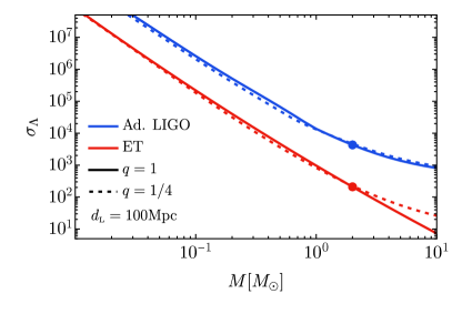
Figure 7: Measurement precision of the deformability parameter $\Lambda$ at both Ad. LIGO and ET. The binary is assumed to have spinless components and negligible eccentricity and deformability, as predicted by the PBH scenario. The solid (dashed) line indicates the result for $q=1$ ($q=1/4$).

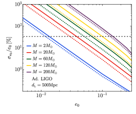
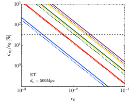
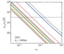
Figure 8: Percentage measurement uncertainty on eccentricity for various values of BBH total mass $M$. The solid, dashed lines correspond to $q=1$ and $q=1/3$, respectively. We can confidently exclude vanishing eccentricity (at 3-$\sigma$ level) below the horizontal gray dashed line. The binaries are assumed to be at a distance of $d_{\text{\tiny\rm L}}=500{\rm Mpc}$ ($100{\rm Mpc}$) for the ground-based (space-based) experiment, respectively. We have checked that varying the BH spins does not significantly affect the eccentricity measurements. Left: Ad. LIGO. Center: ET. Right: LISA.

III.3 Tidal deformability and tidal disruption

In Fig. 7, we show the measurement errors on the binary tidal deformability $\Lambda$ as a function of the total mass $M<10M_{\odot}$, assuming negligible spins, eccentricity, and deformability, as predicted by the PBH scenario. We also report two representative values of the mass ratio ($q=1$ and $q=1/4$), to show its effects of the measurement errors on $\Lambda$. In this case, we show the errors as a function of the binary total mass $M$ and not of the primary mass $m_{1}$, as done in the previous plots. Indeed, we find that $\sigma_{\Lambda}$ depends mostly on $M$.

The typical deformability expected for a BH-NS binary is approximately in the range $\Lambda\in(100,5000)$, depending on the NS equation of state Abbott et al. (2020) and on the mass ratio. Fig. 7 shows that Ad. LIGO (ET) would be able to exclude $\Lambda=0$ at $3\sigma$ (i.e., $\Lambda-3\sigma_{\Lambda}>0$) for a symmetric subsolar-mass binary at $d_{\text{\tiny L}}=100\,{\rm Mpc}$ only if $\Lambda>1.3\times 10^{4}$ ($\Lambda>6.27\times 10^{2}$). Therefore, the constraining power of Ad. LIGO is limited for this discriminator, while ET could exclude the primordial origin of a subsolar-mass binary, based on the tidal deformability measurements, only for the least compact NSs, which are already marginally in tension with GW170817 Abbott et al. (2017a).

Less compact objects like white dwarfs (or hypothetical mini boson stars) have much larger tidal deformability, which can be therefore measured accurately given the estimates in Fig. 7. However, as previously discussed, these objects are tidally disrupted well before the ISCO frequency. In this case the GW signal is abruptly suppressed at the frequency corresponding to the Roche or contact radius, so it can presumably be distinguished more easily from the “smooth” inspiral signal of a BH binary.

For this range of masses the measurement accuracy on $\Lambda$ with LISA is very low, since LISA can only observe the early inspiral and tidal effects enter at high PN order. Therefore, we do not show LISA results in this case.

Finally, note that our Fisher analysis for the errors on $\Lambda$ include the eccentricity in the waveform parameters. We explicitly checked that removing $e$ (i.e. assuming $e=0$ or that it is known a priori) does not affect the error estimates, even though one expects that reducing the dimensionality of the problem would result in better constraining power. This is because the eccentricity and deformability mostly impact separate phases of the inspiral: eccentricity is larger at small frequencies, while the tidal deformability (5PN+) effects become relevant close to the ISCO frequency. Therefore, $e$ and $\Lambda$ are effectively uncorrelated in the Fisher matrix, and removing one of the two parameters does not reduce uncertainties on the other one.

III.4 Eccentricity measurement accuracy

A firm prediction of the scenario involving PBH binaries formed in the early Universe is that their orbit circularizes before entering the observability band of ground-based detectors (see Sec. II.3). In Fig. 8, we show the orbital eccentricity measurement accuracy in Ad. LIGO, ET and, LISA as a function of the binary eccentricity for selected values of the binary masses. Consistently with the results of Ref. Favata et al. (2021) for the case of Ad. LIGO, we find that vanishing eccentricity can be ruled out at 3$\sigma$ level, for a binary with total mass $M$ located at a distance $d_{\text{\tiny L}}=500\,{\rm Mpc}$, if $e_{0}$ is larger than (see also Ref. Lower et al. (2018))

$$e_{0}^{\text{\tiny Ad.~{}LIGO}}\gtrsim 5.5\times 10^{-3}\left(\frac{M}{M_{\odot}}\right)^{0.62},$$ (23)

with only a negligible dependence on the individual spins of the binary components and a minor dependence on the mass ratio. ET will be able to constrain the eccentricity down to lower values, with a minimum resolvable eccentricity scaling with the binary total mass as

$$e_{0}^{\text{\tiny ET}}\gtrsim 1.8\times 10^{-3}\left(\frac{M}{M_{\odot}}\right)^{0.48}.$$ (24)

Finally, assuming a binary located at $d_{\text{\tiny L}}=100$Mpc distance, for LISA one obtains (see also Refs. Nishizawa et al. (2016, 2017))

$$e_{0}^{\text{\tiny LISA}}\gtrsim 1.6\times 10^{-2}\left(\frac{M}{M_{\odot}}\right)^{-0.56}.$$ (25)

It is interesting to stress the trend observed in the relative accuracy as a function of $M$. As the eccentricity decreases during the binary evolution, most of the constraining power comes from low frequencies (see the discussion in Sec. II.3.2). In both the Ad. LIGO and ET cases, a heavier binary enters in the observable frequency band closer to the merger time. For this reason, a larger mass implies larger errors on the eccentricity. On the other hand, LISA is mostly sensitive to smaller frequencies, and larger masses imply smaller errors $\sigma_{e_{0}}$ due both to the wider frequencies observable at fixed observation time, and to the larger SNR. This trend can be observed in the right panel of Fig. 8.

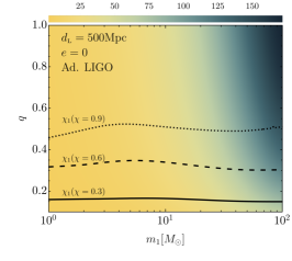
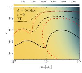
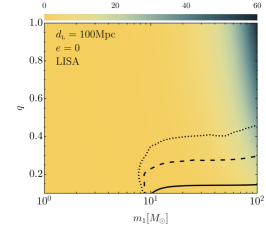
Figure 9: The region below black/red lines indicates the combinations of $(m_{1},q)$ for which one can confidently exclude vanishing spins (at 3-$\sigma$ level) assuming different values of the component BH spins ($\chi_{1}=\chi_{2}=\chi$). The solid, dashed and dotted lines correspond to $\chi=[0.3,0.6,0.9]$, respectively. Black (red) lines correspond to the primary (secondary) BH spins. The color code indicates the SNR, and the source is assumed to be at a distance $d_{\text{\tiny\rm L}}=500$Mpc ($d_{\text{\tiny\rm L}}=100$Mpc) for ground-based (spaced-based) detectors, respectively. Left: Ad. LIGO. Center: ET. Right: LISA.

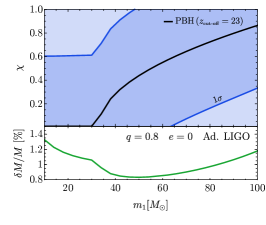
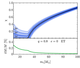
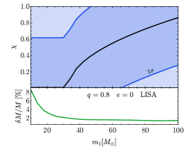
Figure 10: Constraints (at 1, 2, and 3$\sigma$) around the PBH mass-spin correlation of Eq. (II.2) with $z_{\text{\tiny\rm cut-off}}=23$. For illustration, we consider circular binaries with $q=0.8$ at $d_{\text{\tiny L}}=100{\rm Mpc}$. Left: Ad. LIGO. Center: ET. Right: LISA.

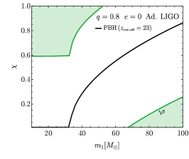
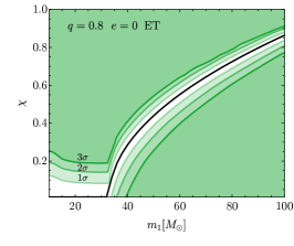
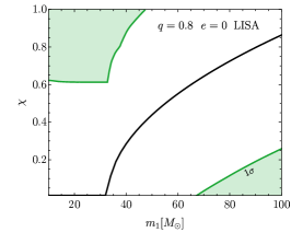
Figure 11: Same as Fig. 10, but we now show in green the region in the $(m_{1},\,\chi)$ parameter space in which we can conclude at 3$\sigma$ C.L. that the event is incompatible with the primordial scenario with $z_{\text{\tiny\rm cut-off}}=23$ (the predicted correlation is shown with a black line). Left: Ad. LIGO. Center: ET. Right: LISA.

III.5 Spin measurement accuracy

In the standard PBH formation scenario, binaries composed of individual PBHs lighter than $m_{\text{\tiny PBH}}\simeq 10M_{\odot}$ retain small spins, as accretion is always ineffective in spinning up individual components (see Sec. II.2). Therefore, measuring a nonzero spin for a sub-10$M_{\odot}$ object would be in tension with a primordial origin (unless we allow for other PBH formation scenarios). At larger masses, the prediction for the spins of primordial binaries becomes uncertain. In particular, binary component spins may still remain negligible up to masses above $m_{\text{\tiny PBH}}\gtrsim 10^{2}M_{\odot}$, provided accretion is inefficient (i.e., with the accretion hyperparameter $z_{\text{\tiny cut-off}}\approx 30$, see Sec. II.2). Therefore, for completeness, we also report whether the spin measurement accuracy is enough to exclude negligible spins in the range of masses $[10,10^{2}]M_{\odot}$. In Sec. III.6 we will address the case of more efficient accretion, and tests of the resulting mass-spin correlation.

In Fig. 9 (left and center panels), we show the parameter space in which Ad. LIGO and ET can confidently exclude negligible spins: i.e. we impose $\chi-3\sigma_{\chi}>0$, so that we can rule out the primordial origin of an event. We place the source at a distance $d_{\text{\tiny L}}=500$ Mpc. The performance of the detectors would, of course, improve for closer sources. Under the assumption of aligned spins, in the limit $q=1$ it is not possible to make independent measurements of the individual component spins. This is because, when setting $q=1$, our waveform model described in App. B.1 is completely determined by $\chi_{s}\equiv(1/2)(\chi_{1}+\chi_{2})$, and the derivative with respect to the antisymmetric spin $\chi_{a}\equiv(1/2)(\chi_{1}-\chi_{2})$ in the Fisher information matrix vanishes identically. Therefore, in this limit, the results of the Fisher analysis only provide the uncertainty on $\chi_{s}$, and there is a complete degeneracy between $\chi_{1}$ and $\chi_{2}$.

In the Ad. LIGO case (left panel), the primary spin can be distinguished from zero for fairly asymmetric sources ($q\lesssim 0.5$) and large primary spin $\chi_{1}\gtrsim 0.3$. On the other hand, the secondary spin is never distinguishable from zero within the 3$\sigma$ confidence limit (C.L.). We can also explain the nearly horizontal behavior of the bound in the $(m_{1},\,q)$ plane. While for a binary located at a fixed distance, larger BBH masses imply larger SNR, they also lead to a smaller number of cycles in the detector band. The two effects compensate each other, giving rise to a comparable spin measurement accuracy in the mass range $m_{\text{\tiny PBH}}\subset[10,10^{2}]M_{\odot}$.

In the ET case (central panel), when $m_{1}\gtrsim 10M_{\odot}$ the larger SNR reduces the error on both spins. We can now rule out negligible primary or secondary spins if the mass ratio is $q\lesssim 0.8$ for $\chi_{1,2}\gtrsim 0.6$. When instead $m_{1}\lesssim 10M_{\odot}$, a primary spin of magnitude $\chi_{1}=[0.3,0.6,0.9]$ can be constrained away from zero if $q\lesssim[0.35,0.6,0.75]$, and the secondary spin is only resolved if $\chi_{2}\gtrsim 0.9$ and $q\lesssim 0.6$.

LISA (right panel) has a smaller reach in this mass range, so we report results for binaries located at a distance $d_{\text{\tiny L}}=100$Mpc. Due to the small SNR, it is not possible to place bounds on the individual spins for primary masses below ${\cal O}(10)M_{\odot}$. For heavier masses, we can only constrained away from zero large primary spins, and only as long as the mass ratio $q\lesssim 0.4$.

III.6 Testing the predicted mass-spin correlations

As discussed in Sec. II.2, accretion effects would imprint a characteristic correlation between masses and spins of PBHs in binaries. If the modelling of PBH accretion is accurate enough, the mass-spin relation can (at least in principle) be compared with a single event to test its consistency with a primordial origin. In this section we forecast the accuracy with which current and future experiments could measure both masses and spins in the range above $m_{1}\gtrsim 10M_{\odot}$, where accretion effects may become relevant. For concreteness, we will fix the hyperparameter $z_{\text{\tiny cut-off}}=23$, motivated by recent comparisons between the PBH scenario and current data Wong et al. (2021); De Luca et al. (2021a); Franciolini et al. (2021), even though different values are still possible. This should only be regarded as illustrative. A more precise determination of $z_{\text{\tiny cut-off}}$ is necessary before the test proposed here can be applied to GW events.

In Fig. 10 we show the accuracy with which various GW detectors could constrain the mass-spin correlation. We assume that we are observing a binary with $q=0.8$, and that the mass-spin correlation is consistent with the predictions of the primordial scenario with $z_{\text{\tiny cut-off}}=23$. The top (bottom) panel shows measurement errors for the individual spins (total mass). For both Ad. LIGO and LISA, the SNR for a source located at $d\text{\tiny L}=100$Mpc is too low to allow for a significant measurement of the individual PBH spins, even though the measurement accuracy on the total mass is rather high. On the contrary, ET will be able to measure the total mass with subpercent accuracy and also to constrain the spin of both individual components, as long as $m_{1}\gtrsim 40M_{\odot}$.

In Fig. 11 we identify the parameter space in the mass-spin plane that is incompatible with the PBH prediction within the GW measurement errors. We inject GW signals in the entire $(m,\,\chi)$ plane, and determine which region can be deemed incompatible with the primordial hypothesis at $3\sigma$. In agreement with the qualitative results in Fig. 10, we find that both Ad. LIGO and LISA will not be able to test the primordial hypothesis on a single-event basis, while ET can place good constraints in most of the parameter space. We conclude that 3G detectors will have large enough SNR to test the primordial hypothesis based on the mass-spin relation, as long as systematic uncertainties in the accretion model are small enough by the time the detectors are taking data.

IV A case study: the GWTC-3 catalog as observed now and by 3G detectors

In this section we apply the algorithm to assess the primordial nature of individual GW sources developed above, and summarized in Fig. 1, to the events reported in the GWTC-3 catalog Abbott et al. (2021b, c). In Sec. IV.1 we ask whether we can draw any conclusion from the observed properties of the GWTC-3 events. Then, in Sec. IV.2, we extrapolate current observations to the estimated measurement accuracy achievable with 3G detectors to understand if any of the current may be confidently classified as primordial (or not) in the near future.

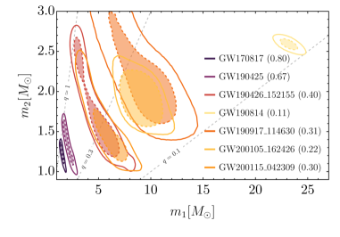
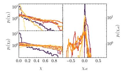
Figure 12: Summary plot showing all 7 events reported in the GWTC-3 catalog having ${\rm FAR}<1/{\rm yr}$ and at least one of the masses below $3M_{\odot}$ Abbott et al. (2021b, c). Left: Posterior distributions in the $(m_{1},m_{2})$ plane. The shaded region corresponds to $50$% C.L., while the outer contour to $90$% C.L. The posterior shapes roughly follow lines of constant chirp mass ${\cal M}$, as that is the best measured parameter from the waveform. To facilitate the discussion in the text, we report the mean value of mass ratio $q$ within brackets on the side of each event’s name. Right: Posterior distributions for both the individual spins $\chi_{i}$ and the effective inspiral spin parameter $\chi_{\text{\tiny\rm eff}}$, following the same color code as in the left panel.

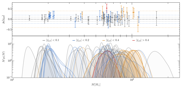
Figure 13: Summary plot showing all 69 events reported in the GWTC-3 catalog having ${\rm FAR}<1/{\rm yr}$ and both masses $\gtrsim 3M_{\odot}$ which are confidently regarded as BBH events Abbott et al. (2021b, c). We show the posterior distribution for the total mass of the binaries (bottom panel), while the color code indicates the mean effective spin parameter. The top panel shows the 90% C.L. for $\chi_{\text{\tiny\rm eff}}$ of each event, following the same color code (the dashed horizontal lines bracket each color group).

IV.1 GWTC-3 events

As the current GW detection horizon is within $z\lesssim 1$, no indication of the primordial nature of the single events can be drawn from current redshift observations.

Additionally, in the GWTC-3 LVK catalog, the eccentricity of the binaries was not measured, as the waveform models used for this analysis work under the assumption of zero eccentricity Abbott et al. (2021b). However, a reanalysis of the events from the O1/O2/O3a runs Romero-Shaw et al. (2021) suggested that GW190521 and GW190620 may present hints of a nonzero eccentricity (see also Romero-Shaw et al. (2019); O’Shea and Kumar (2021); Romero-Shaw et al. (2020); Gayathri et al. (2020); Gamba et al. (2021)). Most of these analyses use waveform models that neglect higher harmonics and spin precession. Since both of these effects are known to be important for an unbiased estimation of the parameters of the binary Romero-Shaw et al. (2020); Hoy et al. (2021), a nonzero eccentricity measurement may still be driven by the inaccuracy of the waveform models. Even if these events are confirmed as having nonzero eccentricity, this would only exclude the primordial origin of two events. In summary, the large majority of the events detected so far has an eccentricity compatible with zero, and therefore this discriminant of their PBH nature is still inconclusive.

As for the tidal deformability, the only LVK event having tidal deformability signatures is GW170817, whose posterior is anyway compatible with $\Lambda\approx 0$. Had the electromagnetic counterpart Abbott et al. (2017b) of this event not been observed, it would have been impossible to confidently rule out the possibility that GW170817 may be a PBH binary, rather than a NS binary.

Short of constraints coming from redshift, eccentricity, and tidal deformabilities, we are left with the masses and spins to test whether the mergers detected so far are of primordial origin. No events with masses below the threshold of $\approx 1M_{\odot}$ have been confidently detected so far, implying that no smoking-gun detection based on light PBH binaries is available  Abbott et al. (2019b); Nitz and Wang (2021a, b); Abbott et al. (2021d).

In Figs. 12 and 13 we show summary plots of the events reported in the GWTC-3 catalog having false-alarm-rate (FAR) above the threshold of $1/{\rm yr}$. We divide the events in the catalog following the analysis in Ref. Abbott et al. (2021c). The first class includes events having at least one object with mass below $\approx 3M_{\odot}$ (potentially consistent with binaries comprising NSs). The second class includes events where both component masses are above $\approx 3M_{\odot}$.

Let us first focus on the distribution of $\chi_{\text{\tiny\rm eff}}$ for the first class. In Fig. 12 (right panel) we clearly see that the distribution of $\chi_{\text{\tiny\rm eff}}$ is mostly peaked around zero. The legend of the left panel of Fig. 12 shows their inferred mass ratio (in round parentheses). At smaller mass ratios the primary spin becomes better constrained: for example, the posterior distribution of GW190814 falls almost entirely within $\chi_{\rm eff}\lesssim 0.1$. Given the small mass ratio and the relatively small total mass, the observed smallness of the primary spin of GW190814 would not be in tension with the primordial scenario even in the presence of strong accretion (say, with $z_{\text{\tiny cut-off}}\approx 10$).

The secondary spin is always mostly unconstrained. A potential exception is GW170817 Abbott et al. (2017a), for which we can infer $\chi_{2}<0.5$ at $90\%$ C.L., mainly because the mass ratio $q$ is close to unity ($m_{1}=1.46^{+0.12}_{-0.10}M_{\odot}$ and $m_{2}=1.27^{+0.09}_{-0.09}M_{\odot}$). Overall, we conclude that it is not possible to rule out the primordial origin of GWTC-3 in the “first class” based only on their mass and spin measurements. The one obvious exception is GW170817, where the observed electromagnetic counterpart Abbott et al. (2017b) (not expected from a BBH merger) allows us to confidently identify the event as a binary NS merger.

Consider now the second class of GWTC-3 events, those for which both masses are above $\approx 3M_{\odot}$ (see Fig. 13). We can further divide these events in two broad categories: one containing events with mean total mass below $\approx 30M_{\odot}$ (corresponding to the first peak in the BBH population distribution identified by the latest LVK population analysis Abbott et al. (2021c)) and the remaining, more massive binaries.

Within the first category, even though no precise measurement of individual spins was performed so far, we can check whether individual events are consistent with the primordial hypothesis by assessing whether $\chi_{\text{\tiny eff}}$ can be compatible with $|\chi_{\text{\tiny eff}}|\lesssim 10^{-2}$, which is the prediction for PBH binaries in this mass range. Out of the 14 events in the first class, five (GW151226, GW190720_000836, GW190728_064510, GW191103_012549, GW191204_171526, and GW191216_213338) have $\chi_{\text{\tiny eff}}>10^{-2}$ at 99% C.L., so they are in tension with the standard PBH scenario.

At larger masses, only three events are found to be spinning (that is, in our context, $|\chi_{\text{\tiny eff}}|\gtrsim 10^{-2}$ at 99% C.L.). The fastest spinning one, GW190517_055101, has $\chi_{\text{\tiny eff}}=0.52_{-0.19}^{+0.19}$, and it could only be compatible with the PBH scenario in the presence of some accretion ($z_{\text{\tiny cut-off}}\lesssim 20$). In addition, due to its smaller total mass, GW190412 would be compatible with the primordial scenario only if $z_{\text{\tiny cut-off}}\lesssim 16$. Finally, the large $|\chi_{\text{\tiny eff}}|$ of GW190519_153544 cannot be used to provide information on its primordial origin because the event has large mass, which would allow for any values of $z_{\text{\tiny cut-off}}$ within the posterior.

Finally, let us focus on the individual spins. Only two out of the 69 massive binaries in the GWTC-3 catalog have primary BH spins incompatible with zero at more than $99\%$ C.L.: these are the aforementioned GW190517_055101 and GW191109_010717. The latter event is “special” also because the posterior for the effective spin $\chi_{\text{\tiny eff}}$ has the largest support at negative values. Given their masses, we can only conclude that these two events would be incompatible with large values of cut-off $z_{\text{\tiny cut-off}}$ (close to $\approx 30$), i.e. with negligible accretion.

We remark that the qualitative analysis of the GWTC-3 events presented in this section is based on the LVK parameter estimation analysis, which assumes uniformative priors. As current detections are still characterized by relatively small SNR values, the interpretation of some events can be sensitive to the choice of priors Pankow et al. (2017); Vitale et al. (2017); Mandel and Fragos (2020); Gerosa et al. (2020); Zevin et al. (2020) (see Ref. Bhagwat et al. (2021) for an interpretation of the events assuming PBH-motivated priors). Additionally, as pointed out by Ref. Romero-Shaw et al. (2021), there is a correlation between the aligned spins and eccentricity obtained from GW parameter estimation. Therefore, GW data analyzed with waveforms neglecting eccentricity may be affected by systematic errors, so that eccentric systems may be misinterpreted as quasicircular systems with nonzero aligned spin.

It was first suggested in Ref. Callister et al. (2021) (and then confirmed in Ref. Abbott et al. (2021c)) that a fraction of the GWTC-3 events shows a peculiar correlation between $q$ and $\chi_{\text{\tiny eff}}$: more asymmetric binaries tend to have larger positive values of $\chi_{\text{\tiny eff}}$. This property of the population cannot conclusively determine the PBH origin of individual events, but the observed correlation would be in contrast with the primordial scenario, which predicts a wider distribution of $\chi_{\text{\tiny eff}}$ for large total masses, and small values of $|\chi_{\text{\tiny eff}}|$ for small $q$ at fixed primary mass. As pointed out in Ref. Franciolini and Pani (2022), GWTC-3 data also support the hypothesis that a fraction of events may be characterized by a mass-spin correlation which closely resembles the one expected in the PBH scenario discussed here. However, the PBH origin of the events is still indistinguishable from astrophysical formation in the dynamical channel with current statistics.

IV.2 GWTC-3-like events as observed by 3G detectors

It is interesting to test whether future experiments would be able to provide enough information to exclude or confirm the primordial origin of some of the GWTC-3 events. We can consider explicit examples and use their inferred parameters in a Fisher matrix analysis to forecast how accurately ET could measure the two individual spins (we neglect $z$, $e$, and $\Lambda$ since, as discussed above, the measured valued for these quantities in the GWTC-3 catalog are uninteresting for ruling out PBHs.)

We consider a representative candidate from each of the various groups of events, including low-mass events, events belonging to the two peaks in the mass distributionidentified in GWTC-3 Abbott et al. (2021c), and upper mass gap events.

Low-mass events (e.g. GW190814). This event is regarded as a potential outlier of both the astrophysical BH and NS populations Abbott et al. (2021c). A similar event detected by ET would have $\mathrm{SNR}\approx 820$, so we would measure the mass parameters with percent precision and the primary spin with $\sigma_{\chi_{1}}\approx 0.04$. This implies that, given the current median value of $\chi_{1}\approx 0.034$, one would not be able to rule out the primordial origin for the primary component of the binary. Because of the small mass ratio, the secondary spin will be poorly measured, with $\sigma_{\chi_{2}}\approx 0.46$. Therefore, it would not be possible to rule out the possibility that the second object may be either a BH formed from stellar collapse, or a second-generation BH resulting from a previous binary NS merger. Similar conclusions apply to GW190917_114630, despite the relatively smaller difference between the individual masses.

First peak in the mass distribution (e.g. GW191204_171526). This is a representative event for the first peak in the BBH mass distribution identified by the LVK population analysis Abbott et al. (2021c), with individual masses $m_{1}=11.9^{+3.3}_{-1.8}M_{\odot}$ and $m_{2}=8.2^{+1.4}_{-1.6}M_{\odot}$. As previously discussed, PBHs with such masses are predicted to retain small spins in the standard scenario. A detection of such an event by ET would have $\mathrm{SNR}\approx 455$ and subpercent precision in measuring mass parameters. The relative errors on the spins would be around $\sigma_{\chi_{1}}\approx 0.16$ and $\sigma_{\chi_{2}}\approx 0.25$, thus allowing us to rule out the primordial origin at $3\sigma$ for similar events with spins larger than $\chi_{1}\gtrsim 0.5$ and $\chi_{2}\gtrsim 0.75$. Ruling out of the primordial origin for events in this region of the parameter space would not be possible with Ad. LIGO. Given the large number of events falling in this mass range, which is currently expected to dominate the BBH population, these findings confirm the importance of 3G detectors for identifying PBH binaries.

Second peak in the mass distribution (e.g. GW200129_ 065458). Similarly to the previous case, we pick this event as representative of the second peak in the BBH mass distribution. In ET this event would have $\mathrm{SNR}\approx 860$, but owing to the larger masses, the spin measurement accuracy is somewhat reduced, with $\sigma_{\chi_{1}}\approx 0.24$ and $\sigma_{\chi_{2}}\approx 0.33$. The reduced spin measurement accuracy and the uncertainties in the accretion model make it challenging to probe the PBH nature of events in this mass range even for ET, unless less distant events are observed (as assumed in Figs. 10 and 11).

Upper mass gap events (e.g. GW190521). Our conclusions on the massive events of the GWTC-3 catalog apply also to GW190521-like objects.

V Conclusions and future work

In previous work we carried out a population analysis and asked whether a subpopulations of PBHs can be compatible with the observed catalog of GW events, given current uncertainties in astrophysical formation scenarios Franciolini et al. (2021). In this work we asked a complementary question: what are the key observables which may allow us to assess the primordial origin of BHs at the single-event level?

We have taken a conservative point of view: we first identified the crucial combinations of binary parameters that would allow us to draw conclusions on the primordial origin of the events, and then we quantified how accurately present and planned experiments (including Ad. LIGO, ET, and LISA) could measure those key observables.

Our findings can be summarized as follows (see Fig. 1):

Large-redshift observations. A smoking-gun signal of PBHs would be the detection of a GW signal at redshift larger than $z\gtrsim 30$, as long as we can confidently set lower bounds on the source redshift. We have estimated uncertainties in the source redshift measurements as a function of the PBH mass, essentially confirming the findings of Ref. Ng et al. (2021). For events at $z>z_{\text{\tiny cut-off}}$ (which might be smaller than $z\approx 30$), another possibility is to use the characteristic $z-\chi$ correlation predicted in the standard PBH formation scenario.

Eccentricity. In the standard formation scenario considered here, primordial binaries do not retain any relevant eccentricity at observable redshifts. We investigated the lower bounds on $e$ above which the primordial nature of the mergers may be excluded. This signature will be useful to rule out the primordial origin of an event only when it retains some significant eccentricity, and even then we should allow for the possibility of an astrophysical origin in dynamical formation scenarios.

Subsolar-mass events and tidal deformability. Even subsolar, zero-eccentricity events may not be PBHs if their tidal deformability is nonzero. Future 3G detectors will be able to measure the mass of BHs in binaries with subpercent accuracy. This is often sufficient to confidently claim the primordial nature of the compact object. Possible alternatives, such as white dwarfs and mini-boson stars, can be distinguished from PBHs by using the characteristic pre-ISCO cut-off in the GW signal caused by tidal disruption.

Masses and spins. We have quantified the mass and spin measurement accuracy achievable by 3G detectors in the solar mass range, showing that ET will be able to test the mass-spin correlation predicted in the standard PBH formation scenario (see Figs. 10 and 11). This test could only be performed on single events in the future if systematic theoretical uncertainties on PBH accretion are significantly reduced.

As a proof of principle, we have applied this strategy to the events in the recently released GWTC-3 catalog. Due to the relatively low SNR of the binary mergers observed in current detectors, there are very few events that can be deemed incompatible with a primordial origin, and there are no smoking-gun signatures of PBHs in the current catalog. We then quantified how 3G detectors will ameliorate the current state of affairs by estimating what could be learned at higher SNRs from the same GW events already present in the GWTC-3 catalog. This is, of course, a very conservative scenario, because the most informative events are likely to be just those that are not observable with current interferometers.

This work can be extended in various directions. It will be interesting to study what can be learned from LISA observations of massive BHs, for which PBH formation predictions are still under investigation, mainly because it is difficult to quantify the effect of accretion. The simple inspiral Fisher matrix analysis we performed can and should be improved through a full Bayesian parameter estimation framework of the complete inspiral-merger-ringdown waveforms (see e.g. Vitale and Evans (2017); Moore and Yunes (2020); Favata et al. (2021); O’Shea and Kumar (2021)). This is especially relevant for low-SNR events. In addition, it is possible that the correlations between certain observable parameters (such as chirp mass and eccentricity) may differ between primordial and astrophysical formation models (see e.g. Breivik et al. (2016)). These correlations may either enhance or reduce the constraining power of future detectors. Finally, it will be interesting to understand how to best optimize the 3G detector network and to investigate the potential of multiband events Sesana (2016); Wong et al. (2018); Cutler et al. (2019); Gerosa et al. (2019); Moore et al. (2019); Ewing et al. (2021); Buscicchio et al. (2021) to better assess the (primordial or astrophysical) nature of the observed merging events.

Table 1: Mass-spin relation for PBH binaries: numerical coefficients in the analytical fit described in Eq. (II.2).

$a^{0}_{1}$	$a^{z,1}_{1}$	$a^{z,2}_{1}$	$a^{z,3}_{1}$	$a^{q,1}_{1}$	$a^{q,2}_{1}$	$a^{q,3}_{1}$	$a^{1,1}_{1}$	$a^{2,1}_{1}$	$a^{1,2}_{1}$	$a^{2,2}_{1}$
$57.8531$	$-66.8879$	$43.9529$	$-5.46522$	$-56.4905$	$39.4605$	$-10.5127$	$37.4532$	$-17.5600$	$-17.5899$	$7.32670$
$b^{0}_{1}$	$b^{z,1}_{1}$	$b^{z,2}_{1}$	$b^{z,3}_{1}$	$b^{q,1}_{1}$	$b^{q,2}_{1}$	$b^{q,3}_{1}$	$b^{1,1}_{1}$	$b^{2,1}_{1}$	$b^{1,2}_{1}$	$b^{2,2}_{1}$
$2.14680$	$-3.65483$	$1.23732$	$-0.185276$	$-1.59262$	$-1.33445$	$0.940219$	$2.48367$	$0.0136971$	$-0.313974$	$-0.218091$
$c^{0}_{1}$	$c^{z,1}_{1}$	$c^{z,2}_{1}$	$c^{z,3}_{1}$	$c^{q,1}_{1}$	$c^{q,2}_{1}$	$c^{q,3}_{1}$	$c^{1,1}_{1}$	$c^{2,1}_{1}$	$c^{1,2}_{1}$	$c^{2,2}_{1}$
$0.441418$	$-0.738179$	$0.834177$	$-0.175491$	$-0.231674$	$2.12451$	$-0.787300$	$-0.0461876$	$-1.20687$	$-0.234563$	$0.477210$
$a^{0}_{2}$	$a^{z,1}_{2}$	$a^{z,2}_{2}$	$a^{z,3}_{2}$	$a^{q,1}_{2}$	$a^{q,2}_{2}$	$a^{q,3}_{2}$	$a^{1,1}_{2}$	$a^{2,1}_{2}$	$a^{1,2}_{2}$	$a^{2,2}_{2}$
$44.3220$	$-72.7617$	$50.9837$	$-8.27027$	$19.8378$	$-33.8142$	$18.3605$	$-6.80676$	$1.95003$	$0.0581762$	$-0.957243$
$b^{0}_{2}$	$b^{z,1}_{2}$	$b^{z,2}_{2}$	$b^{z,3}_{2}$	$b^{q,1}_{2}$	$b^{q,2}_{2}$	$b^{q,3}_{2}$	$b^{1,1}_{2}$	$b^{2,1}_{2}$	$b^{1,2}_{2}$	$b^{2,2}_{2}$
$3.65282$	$-6.94442$	$3.55860$	$-0.630911$	$-0.474109$	$-0.199862$	$0.0523957$	$0.737077$	$0.0855668$	$-0.178022$	$-0.0212303$
$c^{0}_{2}$	$c^{z,1}_{2}$	$c^{z,2}_{2}$	$c^{z,3}_{2}$	$c^{q,1}_{2}$	$c^{q,2}_{2}$	$c^{q,3}_{2}$	$c^{1,1}_{2}$	$c^{2,1}_{2}$	$c^{1,2}_{2}$	$c^{2,2}_{2}$
$-0.189439$	$1.28502$	$-0.587638$	$0.0864602$	$-0.905386$	$1.25085$	$-0.346207$	$0.158765$	$-0.447706$	$-0.0109165$	$0.0945026$

Appendix A Fits of mass-spin relation for PBH binaries as a result of accretion

In this appendix we provide the numerical coefficients specifying the analytical relation between masses and spins for PBH binaries at redshift smaller than $z_{\text{\tiny cut-off}}\in[10,30]$, see Eq. (II.2). These coefficient are reported in Table 1. Mathematica and Python codes with the relevant tabulated functions are publicly available at the GIT repository linked in web . The analytical fit may be useful when performing Bayesian parameter estimations assuming PBH motivated priors, or for searches in the GW catalog for a PBH motivated mass-spin relation.

Appendix B Methodology

In this appendix we review the methodology adopted to derive the main results contained in the paper. We start by reviewing the waveform model we use, mainly following Ref. Favata et al. (2021) and references therein. Then we review the Fisher matrix method and we list our chosen power spectral density curves for the GW experiments discussed in this work, as well as the frequency range used in the integrations.

B.1 Waveform model

We define the GW signal in Fourier space adopting the stationary phase approximation (SPA). We can write

$$\tilde{h}(f)={\mathcal{A}}e^{i\Psi},$$ (26)

where

$${\mathcal{A}}=-\left(\frac{5\pi\eta}{96}\right)^{1/2}\left(\frac{M^{2}}{D}\right)(\pi Mf)^{-7/6}\\ \times\left[(1+\cos^{2}(\iota))^{2}F_{+}^{2}+4\cos^{2}(\iota)F_{\times}^{2}\right]^{1/2}.$$ (27)

Eccentric corrections are only introduced in the phase evolution $\Psi$ via a “post-circular” Yunes and Berti (2008) low-eccentricity expansion accurate to $O(e_{0}^{2})$, presented below. This waveform is an extension of the one presented in Refs. Moore et al. (2016) with the inclusion of spin effects performed in Favata et al. (2021). Also, in the previous formula, we introduced the binary inclination angle $\iota$ relative to the line-of-sight, the distance to the detector $D$, the antenna pattern functions $F_{+,\times}$ and the symmetric mass ratio $\eta=m_{1}m_{2}/M^{2}$. The SPA phase can be written as a sum of PN corrections:

$$\Psi(f)=\phi_{c}+2\pi ft_{c}+\frac{3}{128\eta v^{5}}\Big{(}1+\Delta\Psi^{\text{\tiny tidal}}_{\text{\tiny 6PN}}\\ +\Delta\Psi_{\text{\tiny 3.5PN}}^{\text{\tiny circ.}}+\Delta\Psi_{\text{\tiny 4PN}}^{\text{\tiny spin,circ.}}+\Delta\Psi_{\text{\tiny 3PN}}^{\text{\tiny ecc.}}\Big{)},$$ (28)

where $t_{c}$ and $\phi_{c}$ are the coalescence time and phase, and $v\equiv(\pi Mf)^{1/3}$ is the PN orbital velocity parameter. The tidal deformability terms we include in the waveform, starting at 5PN order, are defined in Eq. (18).

The standard 3.5PN circular contribution is

$$\Delta\Psi_{\text{\tiny 3.5PN}}^{\text{\tiny circ.}}=\sum_{n=2}^{7}c_{n}(\eta)v^{n},$$ (29)

where the coefficients $c_{n}(\eta)$ are found in Eq. (3.18) of Buonanno et al. (2009), and the 2.5PN and 3PN coefficients depend also on $\ln v$.

Spin effects up to 4PN order add a contribution

$$\Delta\Psi_{\text{\tiny 4PN}}^{\text{\tiny spin,circ.}}=4\beta_{1.5}v^{3}-10\sigma v^{4}+v^{5}\ln v^{3}\left[\frac{40}{9}\beta_{2.5}\right.\\ \left.-\beta_{1.5}\left(\frac{3715}{189}+\frac{220}{9}\eta\right)\right]+{\mathcal{P}}_{6}v^{6}+{\mathcal{P}}_{7}v^{7}+{\mathcal{P}}_{8}v^{8},$$ (30)

where $\beta_{1.5}$ is the 1.5PN spin-orbit term Kidder et al. (1993); Poisson (1993); Kidder (1995)

$$\beta_{1.5}=\sum_{i=1,2}\chi_{i}\kappa_{i}\left(\frac{113}{12}\frac{m_{i}^{2}}{M^{2}}+\frac{25}{4}\eta\right).$$ (31)

The 2PN spin-spin term includes three distinct contributions $\sigma=\sigma_{\text{\tiny S}_{1}\text{\tiny S}_{2}}+\sigma_{\text{\tiny QM}}+\sigma_{\text{\tiny self spin}}$ Mikoczi et al. (2005):

i) the standard spin-spin interaction Kidder et al. (1993); Kidder (1995)

$$\sigma_{\text{\tiny S}_{1}\text{\tiny S}_{2}}=\frac{1}{48}\eta\chi_{1}\chi_{2}(721\kappa_{1}\kappa_{2}-247\gamma_{12});$$ (32)

ii) the quadrupole-monopole term Poisson (1998)

$$\sigma_{\text{\tiny QM}} =\frac{5}{2}\sum_{i=1,2}\chi_{i}^{2}\left(\frac{m_{i}}{M}\right)^{2}(3\kappa_{i}^{2}-1);$$ (33)

iii) the self-spin interaction  Mikoczi et al. (2005); Gergely (2000)

$$\sigma_{\text{\tiny SS-self}}=\frac{1}{96}\sum_{i=1,2}\chi_{i}^{2}\left(\frac{m_{i}}{M}\right)^{2}(7-\kappa_{i}^{2}).$$ (34)

In the previous equations $\chi_{i}$ denotes the dimensionless spin parameter, $\kappa_{i}=\hat{{\bm{s}}}_{i}\cdot\hat{{\bm{L}}}_{N}$ is the cosine of the angle between the $i^{\text{\tiny th}}$ spin direction $\hat{{\bm{s}}}_{i}$ and the Newtonian orbital angular momentum direction $\hat{\bm{L}}_{N}$, and $\gamma_{12}={\hat{\bm{s}}}_{1}\cdot{\hat{\bm{s}}}_{2}$.

The 2.5PN spin-orbit term $\beta_{2.5}$ is  Blanchet et al. (2006)

$$\beta^{\text{\tiny SO}}_{2.5}=\sum_{i=1,2}\chi_{i}\kappa_{i}\left[\frac{m_{i}^{2}}{M^{2}}\left(-\frac{31319}{1008}+\frac{1159}{24}\eta\right)\right.$$

$$\left.+\eta\left(-\frac{809}{84}+\frac{281}{8}\eta\right)\right]\;,$$ (35)

where BH absorption terms (i.e., tidal heating) were neglected Alvi (2001). The subsequent 3PN, 3.5PN, and 4PN terms ${\mathcal{P}}_{6}$, ${\mathcal{P}}_{7}$, and ${\mathcal{P}}_{8}$ can be found in Ref. Mishra et al. (2016). This analysis assumes nonprecessing (aligned) spins, and therefore the parameters $\beta_{(\cdots)}$ and $\sigma_{(\cdots)}$ are constant in time and functions of $\chi_{i}$.

Leading-order in eccentricity corrections to the SPA phase were derived up to to 3PN order in Ref. Moore et al. (2016), building upon previous results on eccentric binaries Peters and Mathews (1963b); Junker and Schaefer (1992); Gopakumar et al. (1997); Arun et al. (2008a, b, 2009). Following Ref. Favata et al. (2021), we use the full 3PN expression in our calculations, whose structure is of the form

$$\Delta\Psi_{\text{\tiny 3PN}}^{\text{\tiny ecc.}}=-\frac{2355}{1462}e_{0}^{2}\left(\frac{v_{0}}{v}\right)^{19/3}\left[1+v^{2}\left(\frac{299\,076\,223}{81\,976\,608}\right.\right.$$

$$\left.\left.+\frac{18\,766\,963}{2\,927\,736}\eta\right)+v_{0}^{2}\left(\frac{2833}{1008}-\frac{197}{36}\eta\right)+\cdots+O(v^{6})\right].$$ (36)

Here, $e_{0}$ is the eccentricity at a reference frequency $f_{0}$, and $v_{0}\equiv(\pi Mf_{0})^{1/3}$. The choice of $f_{0}$ is arbitrary, and throughout this paper we set $f_{0}=10$ Hz, following Ref. Favata et al. (2021).

We additionally introduce the effect of cosmological redshift by replacing, in Eq. (26), the distance $D$ by the luminosity distance $d_{\text{\tiny L}}$, defined as

$$d_{\text{\tiny L}}(z)=\frac{c}{H_{0}}(1+z)\int_{0}^{z}\frac{dz^{\prime}}{\sqrt{\Omega_{M}(1+z^{\prime})^{3}+\Omega_{\Lambda}}},$$ (37)

where $H_{0}=100h\,{\rm(km/s)/Mpc}$, $h=0.6790$, $\Omega_{M}=0.3065$, and $\Omega_{\Lambda}=0.6935$  Ade et al. (2016). Also, the redshift of the GW frequency can be accounted for in Eq. (26) by replacing the total mass with the observer-frame total mass $M\rightarrow M_{\text{\tiny obs}}=(1+z)M$. Throughout this work, $M$ refers to the source-frame total mass.

B.2 Fisher matrix analysis

The Fisher information matrix is often used to assess the parameter estimation capabilities of GW detectors (see, for example, Refs. Finn (1992); Finn and Chernoff (1993); Cutler and Flanagan (1994); Poisson and Will (1995); Berti et al. (2005); Ajith and Bose (2009); Cardoso et al. (2017), as well as Refs. Vallisneri (2008); Rodriguez et al. (2013) for discussions of the limitations of this approach).

The output $s(t)$ of a general GW interferometer can be written as the sum of the GW signal $h(t,\vec{\xi})$ and the stationary detector noise $n(t)$. The posterior distribution for the hyperparameters $\vec{\theta}$ can be approximated by

$$p(\vec{\theta}|s)\propto\pi(\vec{\theta})e^{-\frac{1}{2}(h(\vec{\theta})-s|h(\vec{\theta})-s)}$$ (38)

in terms of the prior distribution $\pi(\vec{\theta})$. Here we ahve introduced the inner product

$$(g|h)=2\int_{f_{\text{\tiny min}}}^{f_{\text{\tiny max}}}{\rm d}f\frac{h(f)g^{*}(f)+h^{*}(f)g(f)}{S_{n}(f)}.$$ (39)

In Eq. (39), $S_{n}(f)$ is the detector noise power spectral density, and $f_{\text{\tiny min}}$ ($f_{\text{\tiny max}}$) is the characteristic minimum (maximum) frequency of integration. The frequency band of interest for each GW experiment will be discussed in Sec. B.2.2 below.

Following the principle of the maximum-likelihood estimator, the central values of the hyperparameters are approximated by the point $\vec{\theta}\equiv\vec{\theta}_{\text{\tiny p}}$ where the likelihood peaks. In the limit of large signal-to-noise ratio (SNR$\equiv\sqrt{(h|h)}$), one can perform a Taylor expansion of Eq. (38) and get

$$p(\vec{\theta}|s)\propto\pi(\vec{\theta})e^{-\frac{1}{2}\Gamma_{ab}\Delta\theta^{a}\Delta\theta^{b}},$$ (40)

where $\Delta\vec{\theta}=\vec{\theta}_{\text{\tiny p}}-\vec{\theta}$ and we have introduced the Fisher matrix

$$\Gamma_{ab}=\left(\frac{\partial h}{\partial\theta^{a}}\bigg{|}\frac{\partial h}{\partial\theta^{b}}\right)_{\vec{\theta}=\vec{\theta}_{\text{\tiny p}}}\,.$$ (41)

The errors on the hyperparameters are, therefore, given by $\sigma_{a}=\sqrt{\Sigma^{aa}}$, where $\Sigma^{ab}=\left(\Gamma^{-1}\right)^{ab}$ is the covariance matrix.

Our parameter set is the following:

$$\theta_{a}=(t_{c},\phi_{c},\ln M,\ln\eta,\chi_{1},\chi_{2},\ln e_{0}),$$ (42)

with the addition of the redshift $z$ in Sec. III.1 and of the tidal deformability $\Lambda$ in Sec. III.3. Following Ref. Favata et al. (2021), we use Gaussian priors on the parameters $\phi_{c}\in[-\pi,\pi]$, $\chi_{1,2}\in[-1,1]$, corresponding to

$$\delta\phi_{c}=\pi,\qquad\delta\chi_{1,2}=1,$$ (43)

by adding to the diagonal elements of our Fisher matrix terms of the form $\Gamma^{0}_{aa}=1/(\delta\theta_{a})^{2}$.

Throughout this work, we always consider sources which are optimally oriented with respect to the detector. This means that orientation-dependent terms in the amplitude take the value

$$(1+\cos^{2}(\iota))^{2}F_{+}^{2}+4\cos^{2}(\iota)F_{\times}^{2}=4$$ (44)

and the optimal SNR $\rho_{\text{\tiny opt}}$ can be computed using

$$\rho_{\text{\tiny opt}}^{2}=\frac{5}{6\pi^{4/3}}(1+z)^{5/3}\frac{\eta M^{5/3}}{d_{\text{\tiny L}}^{2}(z)}\int_{f_{\text{\tiny low}}}^{f_{\text{\tiny high}}}\frac{f^{-7/3}}{S_{n}(f)}{\rm d}f.$$ (45)

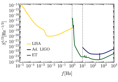
Figure 14: Noise power spectral densities for LISA, ET and Ad. LIGO. The dashed vertical lines indicate the two minimum frequencies for ground-based detectors, i.e. $f_{\text{\tiny\rm low}}^{\text{\tiny\rm Ad. ET}}=1{\rm Hz}$ and $f_{\text{\tiny\rm low}}^{\text{\tiny\rm Ad.~{}LIGO}}=10{\rm Hz}$.

B.2.1 Power spectral density curves

For Ad. LIGO, we consider the expected power spectral density (PSD) of the “zero-detuning, high power” configuration and (2010):

$$S_{n}(f) =10^{-48}{\rm Hz}^{-1}\left(0.0152\,x^{-4}+0.2935\,x^{9/4}\right.$$

$$\left.+2.7951\,x^{3/2}-6.5080\,x^{3/4}+17.7622\right),$$ (46)

where $x=f/(245.4\,{\rm Hz})$ (see also Eq. (4.7) of Ref. Ajith (2011)). We adopt the ET-D sensitivity curves from Ref. Hild et al. (2011). Finally, we consider the LISA PSD of Ref. Robson et al. (2019) (see also Maselli et al. (2021)), that provides an analytic fit for the detector noise. The PSD consists of two parts: the instrumental noise and the confusion noise produced by unresolved galactic binaries, i.e.

$$S_{n}(f)=S^{\textnormal{Ins}}_{n}(f)+S^{\textnormal{WDN}}_{n}(f)\ ,$$ (47)

where

$$S^{\textnormal{Ins}}_{n}(f) =A_{1}\left(P_{\textnormal{OMS}}+2[1+\cos^{2}(f/f_{\star})]\frac{P_{\textnormal{acc}}}{(2\pi f)^{4}}\right)$$

$$\times\left(1+\frac{6}{10}\frac{f^{2}}{f_{\star}^{2}}\right)\ ,$$ (48)

$A_{1}={10}/{3L^{2}}$, $L=2.5$Gm, $f_{\star}=19.09$mHz, while

$$P_{\textnormal{OMS}} =(1.5\times 10^{-11}\textnormal{m})^{2}\left[1+\left(\frac{2\textnormal{mHz}}{f}\right)^{4}\right]\ \textnormal{Hz}^{-1}\ ,$$

$$P_{\textnormal{ACC}} =(3\times 10^{-15}\textnormal{m s}^{-2})^{2}\left[1+\left(\frac{0.4\textnormal{mHz}}{f}\right)^{2}\right]$$

$$\times\left[1+\left(\frac{f}{8\textnormal{mHz}}\right)^{4}\right]\ \textnormal{Hz}^{-1}.$$ (49)

For the white dwarf contribution, we use

$$S^{\textnormal{WDN}}_{n}=A_{2}f^{-7/3}e^{-f^{\alpha}+\beta f\sin(\kappa f)}[1+\tanh(\gamma(f_{k}-f))]\ ,$$ (50)

with the amplitude $A_{2}=9\times 10^{-45}\textnormal{Hz}^{-1}$, and the coefficients $(\alpha,\beta,\kappa,\gamma,f_{k})=(0.171,292,1020,1680,0.00215)$. The noise spectral densities are shown in Fig. 14.

B.2.2 Frequency range

We set $f_{\text{\tiny min}}$ to the minimum frequency detectable by the interferometer. In particular, we adopt as minimum frequencies $f_{\text{\tiny low}}^{\text{\tiny Ad.~{}LIGO}}=10\,{\rm Hz}$ ($f_{\text{\tiny low}}^{\text{\tiny ET}}=1\,{\rm Hz}$) for the Ad. LIGO (ET) case. For LISA we take $f^{\text{\tiny LISA}}_{\text{\tiny low}}={\rm max}[10^{-5}\,{\rm Hz},f^{\text{\tiny LISA}}_{\text{\tiny obs}}$], i.e. the maximum frequency between the cutoff frequency below which the LISA noise curve is not well characterized ($10^{-5}\,{\rm Hz}$) and the frequency corresponding to a binary that spends $T_{\text{\tiny obs}}=1\,{\rm yr}$ to span the frequency band up to $f_{\text{\tiny max}}^{\text{\tiny LISA}}$. We use a LISA maximum frequency $f_{\text{\tiny max}}^{\text{\tiny LISA}}=1\,{\rm Hz}$. Therefore, we find Berti et al. (2005)

$$f^{\text{\tiny LISA}}_{\text{\tiny obs}}=\left[\left(\frac{f_{\text{\tiny max}}^{\text{\tiny LISA}}}{\rm Hz}\right)^{-8/3}+49\left(\frac{\mathcal{M}}{M_{\odot}}\right)^{5/3}\left(\frac{T_{\text{\tiny obs}}}{\rm yr}\right)\right]^{-3/8}\,{\rm Hz}.$$ (51)

On the other hand, the maximum frequency is set by the smallest value between either the maximum frequency reached by the detector

$$f_{\text{\tiny max}}^{\text{(Ad.~{}LIGO,ET,LISA)}}=(10^{4},10^{4},1)\,{\rm Hz}$$ (52)

or the ISCO frequency of the binary system, defined as

$$f_{\text{\tiny ISCO},z}=\frac{1}{1+z}\frac{\hat{\Omega}_{\text{\tiny ISCO}}(\chi_{f})}{\pi M_{f}}\,,$$ (53)

where $\hat{\Omega}_{\text{\tiny ISCO}}(\chi)\equiv M_{\text{\tiny Kerr}}\Omega_{\text{\tiny ISCO}}$ is the dimensionless angular frequency for a circular, equatorial orbit around a Kerr BH with mass $M_{\text{\tiny kerr}}$ and spin parameter $\chi$ Bardeen et al. (1972), while $\chi_{f}$ and $M_{f}$ are the final spin and mass of the BH merger remnant, whose full expressions (based on fits to numerical relativity simulations Husa et al. (2016); Hofmann et al. (2016)) can be found in Appendix B of Ref. Favata et al. (2021).

References

- Zel’dovich and Novikov (1967) Y. B. Zel’dovich and I. D. Novikov, Soviet Astron. AJ (Engl. Transl. ), 10, 602 (1967).
- Hawking (1974) S. W. Hawking, Nature 248, 30 (1974).
- Chapline (1975) G. F. Chapline, Nature 253, 251 (1975).
- Carr (1975) B. J. Carr, Astrophys. J. 201, 1 (1975).
- Ivanov et al. (1994) P. Ivanov, P. Naselsky, and I. Novikov, Phys. Rev. D 50, 7173 (1994).
- Garcia-Bellido et al. (1996) J. Garcia-Bellido, A. D. Linde, and D. Wands, Phys. Rev. D 54, 6040 (1996), arXiv:astro-ph/9605094 .
- Ivanov (1998) P. Ivanov, Phys. Rev. D 57, 7145 (1998), arXiv:astro-ph/9708224 .
- Blinnikov et al. (2016) S. Blinnikov, A. Dolgov, N. K. Porayko, and K. Postnov, JCAP 1611, 036 (2016), arXiv:1611.00541 [astro-ph.HE] .
- Carr et al. (2020) B. Carr, K. Kohri, Y. Sendouda, and J. Yokoyama, (2020), arXiv:2002.12778 [astro-ph.CO] .
- Volonteri (2010) M. Volonteri, "Astronomy and Astrophysics Reviews" 18, 279 (2010), arXiv:1003.4404 [astro-ph.CO] .
- Clesse and García-Bellido (2015) S. Clesse and J. García-Bellido, Phys. Rev. D 92, 023524 (2015), arXiv:1501.07565 [astro-ph.CO] .
- Serpico et al. (2020) P. D. Serpico, V. Poulin, D. Inman, and K. Kohri, Phys. Rev. Res. 2, 023204 (2020), arXiv:2002.10771 [astro-ph.CO] .
- Abbott et al. (2019a) B. P. Abbott et al. (LIGO Scientific, Virgo), Phys. Rev. X 9, 031040 (2019a), arXiv:1811.12907 [astro-ph.HE] .
- Abbott et al. (2021a) R. Abbott et al. (LIGO Scientific, Virgo), Phys. Rev. X 11, 021053 (2021a), arXiv:2010.14527 [gr-qc] .
- Abbott et al. (2021b) R. Abbott et al. (LIGO Scientific, VIRGO, KAGRA), (2021b), arXiv:2111.03606 [gr-qc] .
- Bird et al. (2016) S. Bird, I. Cholis, J. B. Muñoz, Y. Ali-Haïmoud, M. Kamionkowski, E. D. Kovetz, A. Raccanelli, and A. G. Riess, Phys. Rev. Lett. 116, 201301 (2016), arXiv:1603.00464 [astro-ph.CO] .
- Sasaki et al. (2016) M. Sasaki, T. Suyama, T. Tanaka, and S. Yokoyama, Phys. Rev. Lett. 117, 061101 (2016), [erratum: Phys. Rev. Lett.121,no.5,059901(2018)], arXiv:1603.08338 [astro-ph.CO] .
- Eroshenko (2018) Y. N. Eroshenko, J. Phys. Conf. Ser. 1051, 012010 (2018), arXiv:1604.04932 [astro-ph.CO] .
- Wang et al. (2018) S. Wang, Y.-F. Wang, Q.-G. Huang, and T. G. F. Li, Phys. Rev. Lett. 120, 191102 (2018), arXiv:1610.08725 [astro-ph.CO] .
- Ali-Haïmoud et al. (2017) Y. Ali-Haïmoud, E. D. Kovetz, and M. Kamionkowski, Phys. Rev. D96, 123523 (2017), arXiv:1709.06576 [astro-ph.CO] .
- Chen and Huang (2018) Z.-C. Chen and Q.-G. Huang, Astrophys. J. 864, 61 (2018), arXiv:1801.10327 [astro-ph.CO] .
- Raidal et al. (2019) M. Raidal, C. Spethmann, V. Vaskonen, and H. Veermäe, JCAP 02, 018 (2019), arXiv:1812.01930 [astro-ph.CO] .
- Liu et al. (2019a) L. Liu, Z.-K. Guo, and R.-G. Cai, Eur. Phys. J. C 79, 717 (2019a), arXiv:1901.07672 [astro-ph.CO] .
- Hütsi et al. (2019) G. Hütsi, M. Raidal, and H. Veermäe, Phys. Rev. D 100, 083016 (2019), arXiv:1907.06533 [astro-ph.CO] .
- Vaskonen and Veermäe (2020) V. Vaskonen and H. Veermäe, Phys. Rev. D 101, 043015 (2020), arXiv:1908.09752 [astro-ph.CO] .
- Gow et al. (2020) A. D. Gow, C. T. Byrnes, A. Hall, and J. A. Peacock, JCAP 01, 031 (2020), arXiv:1911.12685 [astro-ph.CO] .
- Wu (2020) Y. Wu, Phys. Rev. D101, 083008 (2020), arXiv:2001.03833 [astro-ph.CO] .
- De Luca et al. (2020a) V. De Luca, G. Franciolini, P. Pani, and A. Riotto, JCAP 06, 044 (2020a), arXiv:2005.05641 [astro-ph.CO] .
- Hall et al. (2020) A. Hall, A. D. Gow, and C. T. Byrnes, Phys. Rev. D 102, 123524 (2020), arXiv:2008.13704 [astro-ph.CO] .
- Wong et al. (2021) K. W. K. Wong, G. Franciolini, V. De Luca, V. Baibhav, E. Berti, P. Pani, and A. Riotto, Phys. Rev. D103, 023026 (2021), arXiv:2011.01865 [gr-qc] .
- Hütsi et al. (2021) G. Hütsi, M. Raidal, V. Vaskonen, and H. Veermäe, JCAP 2103, 068 (2021), arXiv:2012.02786 [astro-ph.CO] .
- Kritos et al. (2021) K. Kritos, V. De Luca, G. Franciolini, A. Kehagias, and A. Riotto, JCAP 05, 039 (2021), arXiv:2012.03585 [gr-qc] .
- De Luca et al. (2021a) V. De Luca, G. Franciolini, P. Pani, and A. Riotto, JCAP 05, 003 (2021a), arXiv:2102.03809 [astro-ph.CO] .
- Deng (2021) H. Deng, JCAP 04, 058 (2021), arXiv:2101.11098 [astro-ph.CO] .
- Kimura et al. (2021) R. Kimura, T. Suyama, M. Yamaguchi, and Y.-L. Zhang, JCAP 04, 031 (2021), arXiv:2102.05280 [astro-ph.CO] .
- Franciolini et al. (2021) G. Franciolini, V. Baibhav, V. De Luca, K. K. Y. Ng, K. W. K. Wong, E. Berti, P. Pani, A. Riotto, and S. Vitale, (2021), arXiv:2105.03349 [gr-qc] .
- Bavera et al. (2021) S. S. Bavera, G. Franciolini, G. Cusin, A. Riotto, M. Zevin, and T. Fragos, (2021), arXiv:2109.05836 [astro-ph.CO] .
- Liu et al. (2021) L. Liu, X.-Y. Yang, Z.-K. Guo, and R.-G. Cai, (2021), arXiv:2112.05473 [astro-ph.CO] .
- De Luca et al. (2021b) V. De Luca, G. Franciolini, P. Pani, and A. Riotto, JCAP 11, 039 (2021b), arXiv:2106.13769 [astro-ph.CO] .
- Pujolas et al. (2021) O. Pujolas, V. Vaskonen, and H. Veermäe, Phys. Rev. D 104, 083521 (2021), arXiv:2107.03379 [astro-ph.CO] .
- Abbott et al. (2021c) R. Abbott et al. (LIGO Scientific, VIRGO, KAGRA), (2021c), arXiv:2111.03634 [astro-ph.HE] .
- Sasaki et al. (2018) M. Sasaki, T. Suyama, T. Tanaka, and S. Yokoyama, Class. Quant. Grav. 35, 063001 (2018), arXiv:1801.05235 [astro-ph.CO] .
- Green and Kavanagh (2021) A. M. Green and B. J. Kavanagh, J. Phys. G 48, 4 (2021), arXiv:2007.10722 [astro-ph.CO] .
- Franciolini (2021) G. Franciolini, Primordial Black Holes: from Theory to Gravitational Wave Observations, Other thesis (2021), arXiv:2110.06815 [astro-ph.CO] .
- Clesse and Garcia-Bellido (2020) S. Clesse and J. Garcia-Bellido, (2020), arXiv:2007.06481 [astro-ph.CO] .
- De Luca et al. (2021c) V. De Luca, V. Desjacques, G. Franciolini, P. Pani, and A. Riotto, Phys. Rev. Lett. 126, 051101 (2021c), arXiv:2009.01728 [astro-ph.CO] .
- Bhagwat et al. (2021) S. Bhagwat, V. De Luca, G. Franciolini, P. Pani, and A. Riotto, JCAP 01, 037 (2021), arXiv:2008.12320 [astro-ph.CO] .
- Reitze et al. (2019) D. Reitze et al., Bull. Am. Astron. Soc. 51, 035 (2019), arXiv:1907.04833 [astro-ph.IM] .
- Hild et al. (2011) S. Hild et al., Class. Quant. Grav. 28, 094013 (2011), arXiv:1012.0908 [gr-qc] .
- Amaro-Seoane et al. (2017) P. Amaro-Seoane, H. Audley, S. Babak, J. Baker, E. Barausse, P. Bender, E. Berti, P. Binetruy, M. Born, D. Bortoluzzi, J. Camp, C. Caprini, V. Cardoso, M. Colpi, J. Conklin, N. Cornish, C. Cutler, K. Danzmann, R. Dolesi, L. Ferraioli, V. Ferroni, E. Fitzsimons, J. Gair, L. Gesa Bote, D. Giardini, F. Gibert, C. Grimani, H. Halloin, G. Heinzel, T. Hertog, M. Hewitson, K. Holley-Bockelmann, D. Hollington, M. Hueller, H. Inchauspe, P. Jetzer, N. Karnesis, C. Killow, A. Klein, B. Klipstein, N. Korsakova, S. L. Larson, J. Livas, I. Lloro, N. Man, D. Mance, J. Martino, I. Mateos, K. McKenzie, S. T. McWilliams, C. Miller, G. Mueller, G. Nardini, G. Nelemans, M. Nofrarias, A. Petiteau, P. Pivato, E. Plagnol, E. Porter, J. Reiche, D. Robertson, N. Robertson, E. Rossi, G. Russano, B. Schutz, A. Sesana, D. Shoemaker, J. Slutsky, C. F. Sopuerta, T. Sumner, N. Tamanini, I. Thorpe, M. Troebs, M. Vallisneri, A. Vecchio, D. Vetrugno, S. Vitale, M. Volonteri, G. Wanner, H. Ward, P. Wass, W. Weber, J. Ziemer, and P. Zweifel, arXiv e-prints , arXiv:1702.00786 (2017), arXiv:1702.00786 [astro-ph.IM] .
- Baibhav et al. (2019) V. Baibhav, E. Berti, D. Gerosa, M. Mapelli, N. Giacobbo, Y. Bouffanais, and U. N. Di Carlo, Phys. Rev. D100, 064060 (2019), arXiv:1906.04197 [gr-qc] .
- Maggiore et al. (2020) M. Maggiore et al., JCAP 03, 050 (2020), arXiv:1912.02622 [astro-ph.CO] .
- Kalogera et al. (2021) V. Kalogera et al., (2021), arXiv:2111.06990 [gr-qc] .
- De Luca et al. (2020b) V. De Luca, G. Franciolini, P. Pani, and A. Riotto, JCAP 04, 052 (2020b), arXiv:2003.02778 [astro-ph.CO] .
- Ricotti et al. (2008) M. Ricotti, J. P. Ostriker, and K. J. Mack, Astrophys. J. 680, 829 (2008), arXiv:0709.0524 [astro-ph] .
- Ali-Haïmoud (2018) Y. Ali-Haïmoud, Phys. Rev. Lett. 121, 081304 (2018), arXiv:1805.05912 [astro-ph.CO] .
- Desjacques and Riotto (2018) V. Desjacques and A. Riotto, Phys. Rev. D 98, 123533 (2018), arXiv:1806.10414 [astro-ph.CO] .
- Ballesteros et al. (2018) G. Ballesteros, P. D. Serpico, and M. Taoso, JCAP 10, 043 (2018), arXiv:1807.02084 [astro-ph.CO] .
- Moradinezhad Dizgah et al. (2019) A. Moradinezhad Dizgah, G. Franciolini, and A. Riotto, JCAP 11, 001 (2019), arXiv:1906.08978 [astro-ph.CO] .
- De Luca et al. (2020c) V. De Luca, G. Franciolini, and A. Riotto, Phys. Lett. B807, 135550 (2020c), arXiv:2001.04371 [astro-ph.CO] .
- Nakamura et al. (1997) T. Nakamura, M. Sasaki, T. Tanaka, and K. S. Thorne, Astrophys. J. Lett. 487, L139 (1997), arXiv:astro-ph/9708060 .
- Ioka et al. (1998) K. Ioka, T. Chiba, T. Tanaka, and T. Nakamura, Phys. Rev. D 58, 063003 (1998), arXiv:astro-ph/9807018 .
- Cholis et al. (2016) I. Cholis, E. D. Kovetz, Y. Ali-Haïmoud, S. Bird, M. Kamionkowski, J. B. Muñoz, and A. Raccanelli, Phys. Rev. D 94, 084013 (2016), arXiv:1606.07437 [astro-ph.HE] .
- Raidal et al. (2017) M. Raidal, V. Vaskonen, and H. Veermäe, JCAP 09, 037 (2017), arXiv:1707.01480 [astro-ph.CO] .
- De Luca et al. (2020d) V. De Luca, V. Desjacques, G. Franciolini, and A. Riotto, JCAP 11, 028 (2020d), arXiv:2009.04731 [astro-ph.CO] .
- Schneider et al. (2000) R. Schneider, A. Ferrara, B. Ciardi, V. Ferrari, and S. Matarrese, Mon. Not. Roy. Astron. Soc. 317, 385 (2000), arXiv:astro-ph/9909419 .
- Schneider et al. (2002) R. Schneider, A. Ferrara, P. Natarajan, and K. Omukai, Astrophys. J. 571, 30 (2002), arXiv:astro-ph/0111341 .
- Schneider et al. (2003) R. Schneider, A. Ferrara, R. Salvaterra, K. Omukai, and V. Bromm, Nature 422, 869 (2003), arXiv:astro-ph/0304254 .
- Bromm (2006) V. Bromm, Astrophys. J. 642, 382 (2006), arXiv:astro-ph/0509303 .
- de Souza et al. (2011) R. S. de Souza, N. Yoshida, and K. Ioka, Astron. Astrophys. 533, A32 (2011), arXiv:1105.2395 [astro-ph.CO] .
- Koushiappas and Loeb (2017) S. M. Koushiappas and A. Loeb, Phys. Rev. Lett. 119, 221104 (2017), arXiv:1708.07380 [astro-ph.CO] .
- Mocz et al. (2020) P. Mocz et al., Mon. Not. Roy. Astron. Soc. 494, 2027 (2020), arXiv:1911.05746 [astro-ph.CO] .
- Liu and Bromm (2020a) B. Liu and V. Bromm, Mon. Not. Roy. Astron. Soc. 495, 2475 (2020a), arXiv:2003.00065 [astro-ph.CO] .
- Trenti and Stiavelli (2009) M. Trenti and M. Stiavelli, Astrophys. J. 694, 879 (2009), arXiv:0901.0711 [astro-ph.CO] .
- Tornatore et al. (2007) L. Tornatore, S. Borgani, K. Dolag, and F. Matteucci, Mon. Not. Roy. Astron. Soc. 382, 1050 (2007), arXiv:0705.1921 [astro-ph] .
- Kinugawa et al. (2014) T. Kinugawa, K. Inayoshi, K. Hotokezaka, D. Nakauchi, and T. Nakamura, Mon. Not. Roy. Astron. Soc. 442, 2963 (2014), arXiv:1402.6672 [astro-ph.HE] .
- Kinugawa et al. (2016) T. Kinugawa, A. Miyamoto, N. Kanda, and T. Nakamura, Mon. Not. Roy. Astron. Soc. 456, 1093 (2016), arXiv:1505.06962 [astro-ph.SR] .
- Hartwig et al. (2016) T. Hartwig, M. Volonteri, V. Bromm, R. S. Klessen, E. Barausse, M. Magg, and A. Stacy, Mon. Not. Roy. Astron. Soc. 460, L74 (2016), arXiv:1603.05655 [astro-ph.GA] .
- Belczynski et al. (2017) K. Belczynski, T. Ryu, R. Perna, E. Berti, T. L. Tanaka, and T. Bulik, Mon. Not. Roy. Astron. Soc. 471, 4702 (2017), arXiv:1612.01524 [astro-ph.HE] .
- Inayoshi et al. (2017) K. Inayoshi, R. Hirai, T. Kinugawa, and K. Hotokezaka, Mon. Not. Roy. Astron. Soc. 468, 5020 (2017), arXiv:1701.04823 [astro-ph.HE] .
- Liu and Bromm (2020b) B. Liu and V. Bromm, Astrophys. J. Lett. 903, L40 (2020b), arXiv:2009.11447 [astro-ph.GA] .
- Kinugawa et al. (2020) T. Kinugawa, T. Nakamura, and H. Nakano, Mon. Not. Roy. Astron. Soc. 498, 3946 (2020), arXiv:2005.09795 [astro-ph.HE] .
- Tanikawa et al. (2021) A. Tanikawa, H. Susa, T. Yoshida, A. A. Trani, and T. Kinugawa, Astrophys. J. 910, 30 (2021), arXiv:2008.01890 [astro-ph.HE] .
- Singh et al. (2021) N. Singh, T. Bulik, K. Belczynski, and A. Askar, (2021), arXiv:2112.04058 [astro-ph.HE] .
- Ng et al. (2021) K. K. Y. Ng, S. Chen, B. Goncharov, U. Dupletsa, S. Borhanian, M. Branchesi, J. Harms, M. Maggiore, B. S. Sathyaprakash, and S. Vitale, (2021), arXiv:2108.07276 [astro-ph.CO] .
- Shandera et al. (2018) S. Shandera, D. Jeong, and H. S. G. Gebhardt, Phys. Rev. Lett. 120, 241102 (2018), arXiv:1802.08206 [astro-ph.CO] .
- Cardoso and Pani (2019) V. Cardoso and P. Pani, Living Rev. Rel. 22, 4 (2019), arXiv:1904.05363 [gr-qc] .
- Guo et al. (2019) H.-K. Guo, K. Sinha, and C. Sun, JCAP 09, 032 (2019), arXiv:1904.07871 [hep-ph] .
- Barsanti et al. (2021) S. Barsanti, V. De Luca, A. Maselli, and P. Pani, (2021), arXiv:2109.02170 [gr-qc] .
- Bramante et al. (2018) J. Bramante, T. Linden, and Y.-D. Tsai, Phys. Rev. D 97, 055016 (2018), arXiv:1706.00001 [hep-ph] .
- Takhistov et al. (2021) V. Takhistov, G. M. Fuller, and A. Kusenko, Phys. Rev. Lett. 126, 071101 (2021), arXiv:2008.12780 [astro-ph.HE] .
- Dasgupta et al. (2021) B. Dasgupta, R. Laha, and A. Ray, Phys. Rev. Lett. 126, 141105 (2021), arXiv:2009.01825 [astro-ph.HE] .
- Giffin et al. (2021) P. Giffin, J. Lloyd, S. D. McDermott, and S. Profumo, (2021), arXiv:2105.06504 [hep-ph] .
- Fasano et al. (2020) M. Fasano, K. W. K. Wong, A. Maselli, E. Berti, V. Ferrari, and B. S. Sathyaprakash, Phys. Rev. D 102, 023025 (2020), arXiv:2005.01726 [astro-ph.HE] .
- Hofmann et al. (2016) F. Hofmann, E. Barausse, and L. Rezzolla, Astrophys. J. Lett. 825, L19 (2016), arXiv:1605.01938 [gr-qc] .
- Bardeen et al. (1986) J. M. Bardeen, J. Bond, N. Kaiser, and A. Szalay, Astrophys. J. 304, 15 (1986).
- De Luca et al. (2019) V. De Luca, V. Desjacques, G. Franciolini, A. Malhotra, and A. Riotto, JCAP 05, 018 (2019), arXiv:1903.01179 [astro-ph.CO] .
- Mirbabayi et al. (2020) M. Mirbabayi, A. Gruzinov, and J. Noreña, JCAP 2003, 017 (2020), arXiv:1901.05963 [astro-ph.CO] .
- Ricotti (2007) M. Ricotti, Astrophys. J. 662, 53 (2007), arXiv:0706.0864 [astro-ph] .
- Hasinger (2020) G. Hasinger, (2020), arXiv:2003.05150 [astro-ph.CO] .
- Oh and Haiman (2003) S. P. Oh and Z. Haiman, Mon. Not. Roy. Astron. Soc. 346, 456 (2003), arXiv:astro-ph/0307135 [astro-ph] .
- De Luca et al. (2020e) V. De Luca, G. Franciolini, P. Pani, and A. Riotto, Phys. Rev. D 102, 043505 (2020e), arXiv:2003.12589 [astro-ph.CO] .
- Harada et al. (2017) T. Harada, C.-M. Yoo, K. Kohri, and K.-I. Nakao, Phys. Rev. D 96, 083517 (2017), [Erratum: Phys.Rev.D 99, 069904 (2019)], arXiv:1707.03595 [gr-qc] .
- Flores and Kusenko (2021) M. M. Flores and A. Kusenko, Phys. Rev. D 104, 063008 (2021), arXiv:2106.03237 [astro-ph.CO] .
- Dvali et al. (2021) G. Dvali, F. Kühnel, and M. Zantedeschi, (2021), arXiv:2108.09471 [hep-ph] .
- Eroshenko (2021) Y. N. Eroshenko, (2021), arXiv:2111.03403 [astro-ph.CO] .
- De Luca et al. (2021d) V. De Luca, G. Franciolini, A. Kehagias, P. Pani, and A. Riotto, (2021d), arXiv:2112.02534 [astro-ph.CO] .
- Wang and Nitz (2021) Y.-F. Wang and A. H. Nitz, Astrophys. J. 912, 53 (2021), arXiv:2101.12269 [astro-ph.HE] .
- Kavanagh et al. (2018) B. J. Kavanagh, D. Gaggero, and G. Bertone, Phys. Rev. D 98, 023536 (2018), arXiv:1805.09034 [astro-ph.CO] .
- Liu et al. (2019b) L. Liu, Z.-K. Guo, and R.-G. Cai, Phys. Rev. D 99, 063523 (2019b), arXiv:1812.05376 [astro-ph.CO] .
- Peters and Mathews (1963a) P. C. Peters and J. Mathews, Phys. Rev. 131, 435 (1963a).
- Peters (1964) P. C. Peters, Phys. Rev. 136, B1224 (1964).
- Mandel (2021) I. Mandel, (2021), arXiv:2110.09254 [astro-ph.HE] .
- Maggiore (2007) M. Maggiore, Gravitational Waves. Vol. 1: Theory and Experiments, Oxford Master Series in Physics (Oxford University Press, 2007).
- Pannarale et al. (2015) F. Pannarale, E. Berti, K. Kyutoku, B. D. Lackey, and M. Shibata, Phys. Rev. D 92, 081504 (2015), arXiv:1509.06209 [gr-qc] .
- Kowalska et al. (2011) I. Kowalska, T. Bulik, K. Belczynski, M. Dominik, and D. Gondek-Rosinska, "Astronomy and Astrophysics" 527, A70 (2011), arXiv:1010.0511 [astro-ph.CO] .
- Kyutoku and Seto (2016) K. Kyutoku and N. Seto, Mon. Not. Roy. Astron. Soc. 462, 2177 (2016), arXiv:1606.02298 [astro-ph.HE] .
- Samsing et al. (2014) J. Samsing, M. MacLeod, and E. Ramirez-Ruiz, Astrophys. J. 784, 71 (2014), arXiv:1308.2964 [astro-ph.HE] .
- Nishizawa et al. (2016) A. Nishizawa, E. Berti, A. Klein, and A. Sesana, Phys. Rev. D 94, 064020 (2016), arXiv:1605.01341 [gr-qc] .
- Breivik et al. (2016) K. Breivik, C. L. Rodriguez, S. L. Larson, V. Kalogera, and F. A. Rasio, Astrophys. J. Lett. 830, L18 (2016), arXiv:1606.09558 [astro-ph.GA] .
- Nishizawa et al. (2017) A. Nishizawa, A. Sesana, E. Berti, and A. Klein, Mon. Not. Roy. Astron. Soc. 465, 4375 (2017), arXiv:1606.09295 [astro-ph.HE] .
- Zevin et al. (2021) M. Zevin, I. M. Romero-Shaw, K. Kremer, E. Thrane, and P. D. Lasky, (2021), arXiv:2106.09042 [astro-ph.HE] .
- Jedamzik (2020) K. Jedamzik, JCAP 09, 022 (2020), arXiv:2006.11172 [astro-ph.CO] .
- Trashorras et al. (2021) M. Trashorras, J. García-Bellido, and S. Nesseris, Universe 7, 18 (2021), arXiv:2006.15018 [astro-ph.CO] .
- Kilic et al. (2007) M. Kilic, C. Allende Prieto, W. R. Brown, and D. Koester, Astrophys. J. 660, 1451 (2007), arXiv:astro-ph/0611498 .
- Strobel et al. (1999) K. Strobel, C. Schaab, and M. K. Weigel, Astron. Astrophys. 350, 497 (1999), arXiv:astro-ph/9908132 .
- Lattimer (2012) J. M. Lattimer, Ann. Rev. Nucl. Part. Sci. 62, 485 (2012), arXiv:1305.3510 [nucl-th] .
- Silva et al. (2016) H. O. Silva, H. Sotani, and E. Berti, Mon. Not. Roy. Astron. Soc. 459, 4378 (2016), arXiv:1601.03407 [astro-ph.HE] .
- Suwa et al. (2018) Y. Suwa, T. Yoshida, M. Shibata, H. Umeda, and K. Takahashi, Mon. Not. Roy. Astron. Soc. 481, 3305 (2018), arXiv:1808.02328 [astro-ph.HE] .
- Liebling and Palenzuela (2012) S. L. Liebling and C. Palenzuela, Living Rev. Rel. 15, 6 (2012), arXiv:1202.5809 [gr-qc] .
- Cardoso et al. (2017) V. Cardoso, E. Franzin, A. Maselli, P. Pani, and G. Raposo, Phys. Rev. D 95, 084014 (2017), [Addendum: Phys.Rev.D 95, 089901 (2017)], arXiv:1701.01116 [gr-qc] .
- Ruffini and Bonazzola (1969) R. Ruffini and S. Bonazzola, Phys. Rev. 187, 1767 (1969).
- Colpi et al. (1986) M. Colpi, S. L. Shapiro, and I. Wasserman, Phys. Rev. Lett. 57, 2485 (1986).
- Binnington and Poisson (2009) T. Binnington and E. Poisson, Phys. Rev. D 80, 084018 (2009), arXiv:0906.1366 [gr-qc] .
- Damour and Nagar (2009) T. Damour and A. Nagar, Phys. Rev. D 80, 084035 (2009), arXiv:0906.0096 [gr-qc] .
- Damour and Lecian (2009) T. Damour and O. M. Lecian, Phys. Rev. D 80, 044017 (2009), arXiv:0906.3003 [gr-qc] .
- Pani et al. (2015a) P. Pani, L. Gualtieri, A. Maselli, and V. Ferrari, Phys. Rev. D 92, 024010 (2015a), arXiv:1503.07365 [gr-qc] .
- Pani et al. (2015b) P. Pani, L. Gualtieri, and V. Ferrari, Phys. Rev. D 92, 124003 (2015b), arXiv:1509.02171 [gr-qc] .
- Gürlebeck (2015) N. Gürlebeck, Phys. Rev. Lett. 114, 151102 (2015), arXiv:1503.03240 [gr-qc] .
- Porto (2016) R. A. Porto, Fortsch. Phys. 64, 723 (2016), arXiv:1606.08895 [gr-qc] .
- Le Tiec and Casals (2021) A. Le Tiec and M. Casals, Phys. Rev. Lett. 126, 131102 (2021), arXiv:2007.00214 [gr-qc] .
- Chia (2020) H. S. Chia, (2020), arXiv:2010.07300 [gr-qc] .
- Le Tiec et al. (2021) A. Le Tiec, M. Casals, and E. Franzin, Phys. Rev. D 103, 084021 (2021), arXiv:2010.15795 [gr-qc] .
- Hui et al. (2021) L. Hui, A. Joyce, R. Penco, L. Santoni, and A. R. Solomon, JCAP 04, 052 (2021), arXiv:2010.00593 [hep-th] .
- Charalambous et al. (2021a) P. Charalambous, S. Dubovsky, and M. M. Ivanov, Phys. Rev. Lett. 127, 101101 (2021a), arXiv:2103.01234 [hep-th] .
- Charalambous et al. (2021b) P. Charalambous, S. Dubovsky, and M. M. Ivanov, JHEP 05, 038 (2021b), arXiv:2102.08917 [hep-th] .
- Pereñiguez and Cardoso (2021) D. Pereñiguez and V. Cardoso, (2021), arXiv:2112.08400 [gr-qc] .
- Flanagan and Hinderer (2008) E. E. Flanagan and T. Hinderer, Phys. Rev. D 77, 021502 (2008), arXiv:0709.1915 [astro-ph] .
- Vines et al. (2011) J. Vines, E. E. Flanagan, and T. Hinderer, Phys. Rev. D 83, 084051 (2011), arXiv:1101.1673 [gr-qc] .
- Poisson and Will (1953) E. Poisson and C. Will, Gravity: Newtonian, Post-Newtonian, Relativistic (Cambridge University Press, Cambridge, UK, 1953).
- Cardoso and Duque (2020) V. Cardoso and F. Duque, Phys. Rev. D 101, 064028 (2020), arXiv:1912.07616 [gr-qc] .
- De Luca and Pani (2021) V. De Luca and P. Pani, JCAP 08, 032 (2021), arXiv:2106.14428 [gr-qc] .
- Alvi (2001) K. Alvi, Phys. Rev. D 64, 104020 (2001), arXiv:gr-qc/0107080 .
- Maselli et al. (2018) A. Maselli, P. Pani, V. Cardoso, T. Abdelsalhin, L. Gualtieri, and V. Ferrari, Phys. Rev. Lett. 120, 081101 (2018), arXiv:1703.10612 [gr-qc] .
- Vallisneri (2008) M. Vallisneri, Phys. Rev. D 77, 042001 (2008), arXiv:gr-qc/0703086 .
- Robson et al. (2019) T. Robson, N. J. Cornish, and C. Liu, Class. Quant. Grav. 36, 105011 (2019), arXiv:1803.01944 [astro-ph.HE] .
- Kaiser and McWilliams (2021) A. R. Kaiser and S. T. McWilliams, Class. Quant. Grav. 38, 055009 (2021), arXiv:2010.02135 [gr-qc] .
- Abbott et al. (2020) B. P. Abbott et al. (LIGO Scientific, Virgo), Class. Quant. Grav. 37, 045006 (2020), arXiv:1908.01012 [gr-qc] .
- Pacilio et al. (2021) C. Pacilio, A. Maselli, M. Fasano, and P. Pani, (2021), arXiv:2104.10035 [gr-qc] .
- Favata (2014) M. Favata, Phys. Rev. Lett. 112, 101101 (2014), arXiv:1310.8288 [gr-qc] .
- Abbott et al. (2017a) B. P. Abbott et al. (LIGO Scientific, Virgo), Phys. Rev. Lett. 119, 161101 (2017a), arXiv:1710.05832 [gr-qc] .
- Favata et al. (2021) M. Favata, C. Kim, K. G. Arun, J. Kim, and H. W. Lee, (2021), arXiv:2108.05861 [gr-qc] .
- Lower et al. (2018) M. E. Lower, E. Thrane, P. D. Lasky, and R. Smith, Phys. Rev. D98, 083028 (2018), arXiv:1806.05350 [astro-ph.HE] .
- Romero-Shaw et al. (2021) I. M. Romero-Shaw, P. D. Lasky, and E. Thrane, Astrophys. J. Lett. 921, L31 (2021), arXiv:2108.01284 [astro-ph.HE] .
- Romero-Shaw et al. (2019) I. M. Romero-Shaw, P. D. Lasky, and E. Thrane, Monthly Notices of the Royal Astronomical Society 490, 5210 (2019), https://academic.oup.com/mnras/article-pdf/490/4/5210/30725872/stz2996.pdf .
- O’Shea and Kumar (2021) E. O’Shea and P. Kumar, (2021), arXiv:2107.07981 [astro-ph.HE] .
- Romero-Shaw et al. (2020) I. M. Romero-Shaw, P. D. Lasky, E. Thrane, and J. C. Bustillo, Astrophys. J. Lett. 903, L5 (2020), arXiv:2009.04771 [astro-ph.HE] .
- Gayathri et al. (2020) V. Gayathri, J. Healy, J. Lange, B. O’Brien, M. Szczepanczyk, I. Bartos, M. Campanelli, S. Klimenko, C. Lousto, and R. O’Shaughnessy, (2020), arXiv:2009.05461 [astro-ph.HE] .
- Gamba et al. (2021) R. Gamba, M. Breschi, G. Carullo, P. Rettegno, S. Albanesi, S. Bernuzzi, and A. Nagar, (2021), arXiv:2106.05575 [gr-qc] .
- Hoy et al. (2021) C. Hoy, C. Mills, and S. Fairhurst, (2021), arXiv:2111.10455 [gr-qc] .
- Abbott et al. (2017b) B. P. Abbott et al. (LIGO Scientific, Virgo, Fermi GBM, INTEGRAL, IceCube, AstroSat Cadmium Zinc Telluride Imager Team, IPN, Insight-Hxmt, ANTARES, Swift, AGILE Team, 1M2H Team, Dark Energy Camera GW-EM, DES, DLT40, GRAWITA, Fermi-LAT, ATCA, ASKAP, Las Cumbres Observatory Group, OzGrav, DWF (Deeper Wider Faster Program), AST3, CAASTRO, VINROUGE, MASTER, J-GEM, GROWTH, JAGWAR, CaltechNRAO, TTU-NRAO, NuSTAR, Pan-STARRS, MAXI Team, TZAC Consortium, KU, Nordic Optical Telescope, ePESSTO, GROND, Texas Tech University, SALT Group, TOROS, BOOTES, MWA, CALET, IKI-GW Follow-up, H.E.S.S., LOFAR, LWA, HAWC, Pierre Auger, ALMA, Euro VLBI Team, Pi of Sky, Chandra Team at McGill University, DFN, ATLAS Telescopes, High Time Resolution Universe Survey, RIMAS, RATIR, SKA South Africa/MeerKAT), Astrophys. J. Lett. 848, L12 (2017b), arXiv:1710.05833 [astro-ph.HE] .
- Abbott et al. (2019b) B. P. Abbott et al. (LIGO Scientific, Virgo), Phys. Rev. Lett. 123, 161102 (2019b), arXiv:1904.08976 [astro-ph.CO] .
- Nitz and Wang (2021a) A. H. Nitz and Y.-F. Wang, (2021a), 10.3847/1538-4357/ac01d9, arXiv:2102.00868 [astro-ph.HE] .
- Nitz and Wang (2021b) A. H. Nitz and Y.-F. Wang, Phys. Rev. Lett. 127, 151101 (2021b), arXiv:2106.08979 [astro-ph.HE] .
- Abbott et al. (2021d) R. Abbott et al. (LIGO Scientific, VIRGO, KAGRA), (2021d), arXiv:2109.12197 [astro-ph.CO] .
- Graham et al. (2020) M. J. Graham et al., Phys. Rev. Lett. 124, 251102 (2020), arXiv:2006.14122 [astro-ph.HE] .
- Tsai et al. (2020) Y.-D. Tsai, A. Palmese, S. Profumo, and T. Jeltema, (2020), 10.1088/1475-7516/2021/10/019, arXiv:2007.03686 [astro-ph.HE] .
- Sasaki et al. (2021) M. Sasaki, V. Takhistov, V. Vardanyan, and Y.-l. Zhang, (2021), arXiv:2110.09509 [astro-ph.CO] .
- Kritos and Cholis (2021) K. Kritos and I. Cholis, Phys. Rev. D 104, 043004 (2021), arXiv:2104.02073 [astro-ph.GA] .
- Pankow et al. (2017) C. Pankow, L. Sampson, L. Perri, E. Chase, S. Coughlin, M. Zevin, and V. Kalogera, Astrophys. J. 834, 154 (2017), arXiv:1610.05633 [astro-ph.HE] .
- Vitale et al. (2017) S. Vitale, D. Gerosa, C.-J. Haster, K. Chatziioannou, and A. Zimmerman, Phys. Rev. Lett. 119, 251103 (2017), arXiv:1707.04637 [gr-qc] .
- Mandel and Fragos (2020) I. Mandel and T. Fragos, Astrophys. J. Lett. 895, L28 (2020), arXiv:2004.09288 [astro-ph.HE] .
- Gerosa et al. (2020) D. Gerosa, S. Vitale, and E. Berti, Phys. Rev. Lett. 125, 101103 (2020), arXiv:2005.04243 [astro-ph.HE] .
- Zevin et al. (2020) M. Zevin, C. P. L. Berry, S. Coughlin, K. Chatziioannou, and S. Vitale, Astrophys. J. Lett. 899, L17 (2020), arXiv:2006.11293 [astro-ph.HE] .
- Callister et al. (2021) T. A. Callister, C.-J. Haster, K. K. Y. Ng, S. Vitale, and W. M. Farr, Astrophys. J. Lett. 922, L5 (2021), arXiv:2106.00521 [astro-ph.HE] .
- Franciolini and Pani (2022) G. Franciolini and P. Pani, (2022), arXiv:2201.13098 [astro-ph.HE] .
- Vitale and Evans (2017) S. Vitale and M. Evans, Phys. Rev. D 95, 064052 (2017), arXiv:1610.06917 [gr-qc] .
- Moore and Yunes (2020) B. Moore and N. Yunes, Class. Quant. Grav. 37, 225015 (2020), arXiv:1910.01680 [gr-qc] .
- Sesana (2016) A. Sesana, Phys. Rev. Lett. 116, 231102 (2016), arXiv:1602.06951 [gr-qc] .
- Wong et al. (2018) K. W. K. Wong, E. D. Kovetz, C. Cutler, and E. Berti, Phys. Rev. Lett. 121, 251102 (2018), arXiv:1808.08247 [astro-ph.HE] .
- Cutler et al. (2019) C. Cutler et al., (2019), arXiv:1903.04069 [astro-ph.HE] .
- Gerosa et al. (2019) D. Gerosa, S. Ma, K. W. K. Wong, E. Berti, R. O’Shaughnessy, Y. Chen, and K. Belczynski, Phys. Rev. D 99, 103004 (2019), arXiv:1902.00021 [astro-ph.HE] .
- Moore et al. (2019) C. J. Moore, D. Gerosa, and A. Klein, Mon. Not. Roy. Astron. Soc. 488, L94 (2019), arXiv:1905.11998 [astro-ph.HE] .
- Ewing et al. (2021) B. Ewing, S. Sachdev, S. Borhanian, and B. S. Sathyaprakash, Phys. Rev. D 103, 023025 (2021), arXiv:2011.03036 [gr-qc] .
- Buscicchio et al. (2021) R. Buscicchio, A. Klein, E. Roebber, C. J. Moore, D. Gerosa, E. Finch, and A. Vecchio, Phys. Rev. D 104, 044065 (2021), arXiv:2106.05259 [astro-ph.HE] .
- (196) https://web.uniroma1.it/gmunu/.
- Yunes and Berti (2008) N. Yunes and E. Berti, Phys. Rev. D 77, 124006 (2008), [Erratum: Phys.Rev.D 83, 109901 (2011)], arXiv:0803.1853 [gr-qc] .
- Moore et al. (2016) B. Moore, M. Favata, K. G. Arun, and C. K. Mishra, Phys. Rev. D 93, 124061 (2016), arXiv:1605.00304 [gr-qc] .
- Buonanno et al. (2009) A. Buonanno, B. R. Iyer, E. Ochsner, Y. Pan, and B. S. Sathyaprakash, Phys. Rev. D 80, 084043 (2009).
- Kidder et al. (1993) L. E. Kidder, C. M. Will, and A. G. Wiseman, Phys. Rev. D 47, R4183 (1993), arXiv:gr-qc/9211025 .
- Poisson (1993) E. Poisson, Phys. Rev. D 48, 1860 (1993).
- Kidder (1995) L. E. Kidder, Phys. Rev. D 52, 821 (1995), arXiv:gr-qc/9506022 .
- Mikoczi et al. (2005) B. Mikoczi, M. Vasuth, and L. A. Gergely, Phys. Rev. D 71, 124043 (2005), arXiv:astro-ph/0504538 .
- Poisson (1998) E. Poisson, Phys. Rev. D 57, 5287 (1998), arXiv:gr-qc/9709032 .
- Gergely (2000) L. A. Gergely, Phys. Rev. D 61, 024035 (2000), arXiv:gr-qc/9911082 .
- Blanchet et al. (2006) L. Blanchet, A. Buonanno, and G. Faye, Phys. Rev. D 74, 104034 (2006).
- Mishra et al. (2016) C. K. Mishra, A. Kela, K. G. Arun, and G. Faye, Phys. Rev. D 93, 084054 (2016), arXiv:1601.05588 [gr-qc] .
- Peters and Mathews (1963b) P. C. Peters and J. Mathews, Phys. Rev. 131, 435 (1963b).
- Junker and Schaefer (1992) W. Junker and G. Schaefer, "Mon. Not. Roy. Astron. Soc." 254, 146 (1992).
- Gopakumar et al. (1997) A. Gopakumar, B. R. Iyer, and S. Iyer, Phys. Rev. D 55, 6030 (1997), [Erratum: Phys.Rev.D 57, 6562 (1998)], arXiv:gr-qc/9703075 .
- Arun et al. (2008a) K. G. Arun, L. Blanchet, B. R. Iyer, and M. S. S. Qusailah, Phys. Rev. D 77, 064034 (2008a), arXiv:0711.0250 [gr-qc] .
- Arun et al. (2008b) K. G. Arun, L. Blanchet, B. R. Iyer, and M. S. S. Qusailah, Phys. Rev. D 77, 064035 (2008b), arXiv:0711.0302 [gr-qc] .
- Arun et al. (2009) K. G. Arun, L. Blanchet, B. R. Iyer, and S. Sinha, Phys. Rev. D 80, 124018 (2009), arXiv:0908.3854 [gr-qc] .
- Ade et al. (2016) P. A. R. Ade et al. (Planck), Astron. Astrophys. 594, A13 (2016), arXiv:1502.01589 [astro-ph.CO] .
- Finn (1992) L. S. Finn, Phys. Rev. D 46, 5236 (1992).
- Finn and Chernoff (1993) L. S. Finn and D. F. Chernoff, Phys. Rev. D 47, 2198 (1993).
- Cutler and Flanagan (1994) C. Cutler and E. E. Flanagan, Phys. Rev. D 49, 2658 (1994), arXiv:gr-qc/9402014 .
- Poisson and Will (1995) E. Poisson and C. M. Will, Phys. Rev. D 52, 848 (1995), arXiv:gr-qc/9502040 .
- Berti et al. (2005) E. Berti, A. Buonanno, and C. M. Will, Phys. Rev. D 71, 084025 (2005), arXiv:gr-qc/0411129 .
- Ajith and Bose (2009) P. Ajith and S. Bose, Phys. Rev. D 79, 084032 (2009), arXiv:0901.4936 [gr-qc] .
- Rodriguez et al. (2013) C. L. Rodriguez, B. Farr, W. M. Farr, and I. Mandel, Phys. Rev. D 88, 084013 (2013), arXiv:1308.1397 [astro-ph.IM] .
- and (2010) G. M. H. and, Classical and Quantum Gravity 27, 084006 (2010).
- Ajith (2011) P. Ajith, Phys. Rev. D 84, 084037 (2011), arXiv:1107.1267 [gr-qc] .
- Maselli et al. (2021) A. Maselli, N. Franchini, L. Gualtieri, T. P. Sotiriou, S. Barsanti, and P. Pani, (2021), arXiv:2106.11325 [gr-qc] .
- Bardeen et al. (1972) J. M. Bardeen, W. H. Press, and S. A. Teukolsky, Astrophys. J. 178, 347 (1972).
- Husa et al. (2016) S. Husa, S. Khan, M. Hannam, M. Pürrer, F. Ohme, X. Jiménez Forteza, and A. Bohé, Phys. Rev. D 93, 044006 (2016), arXiv:1508.07250 [gr-qc] .