Mitigation of Crosstalk Errors in a Quantum Measurement and Its Applications

Abstract

In practical realizations of quantum information processing, there may exist noise in a measurement readout stage where errors appear not only on individual qubits but also on multiple ones collectively, the latter of which is called crosstalk errors. In this work, we present a framework for mitigating measurement errors, for both individual and crosstalk errors. The mitigation protocol consists of two steps, firstly quantum pre-processing, which applies local unitary transformations before a measurement, and classical post-processing that manipulates measurement outcomes to recover noiseless data. The local unitaries in quantum pre-processing can be constructed by characterizing a noisy measurement via quantum detector tomography. We show that the mitigation protocol can maintain a measurement error on multiple qubits as much as that in a single-qubit readout, i.e., the error rates for measurements on multiple qubits are suppressed up to a percent level. The mitigation protocol is realized in IBMQ Sydney and applied to the certification of entanglement-generating circuits. It is demonstrated that the mitigation protocol can successfully eliminate measurement errors so that entanglement-generation circuits can be efficiently certified.

Introduction. One of the challenges to facilitate quantum information processing for practical applications is to clear noise appearing in actual implementation. For a quantum circuit, i.e., during quantum dynamics, an ultimate method to defeat all types of noise in a fault-tolerant manner could be offered by quantum error-correcting codes Shor (1995); Gottesman (1997); Kempe (2007). The present-day quantum technologies referred to as noisy intermediate-scale quantum (NISQ) systems Preskill (2018) are not yet capable of realizing quantum error correction, for which it is essential to implement quantum operations with sufficiently high precision. Meanwhile, a cost-effective and suboptimal strategy is to realize error mitigation whereby the effect of noise could be suppressed, e.g., see also recent reviews McClean et al. (2016); Endo et al. (2021); Cerezo et al. (2020); Bharti et al. (2021). Quantum error mitigation would make it possible to achieve desired quantum information processing even if noise is yet present. Various methods along the line are proposed, e.g., Endo et al. (2018); Temme et al. (2017); Li and Benjamin (2017); McClean et al. (2020); McArdle et al. (2019); Maciejewski et al. (2020); Kwon and Bae (2020).

A challenging problem along the line is to understand and characterize noise arising in NISQ systems. In fact, the problem is not only of practical interest for devising methods of error mitigation but also of fundamental importance toward understanding quantum noise. In particular, crosstalk errors may appear due to interactions among systems of interest, but not an environment, and its presence is also evidenced Chen et al. (2019); Rudinger et al. (2021). Crosstalk errors may have different origins and appear in various types Sarovar et al. (2020). Moreover, some crosstalk noise is also endemic at specific physical systems such as superconducting qubits or trapped ions Parrado-Rodríguez et al. (2020). For these reasons, a specific property found in a NISQ system concerning crosstalk errors cannot be thus generalized.

It turns out that crosstalk errors also exist in measurement readout Chen et al. (2019); Lienhard et al. (2021); Seo and Bae (2021). It is clear that quantum error-correcting codes that ultimately fix all types of errors appearing in a circuit do not work for measurement errors. So far, there have been approaches for mitigating errors in individual measurements Maciejewski et al. (2020); Kwon and Bae (2020); Wang et al. (2021); Geller (2020, 2021). Although single-qubit readout has an error in a percent level, crosstalk can significantly increase an error rate on multiple qubits Seo and Bae (2021). Very recently, crosstalk errors in quantum measurements are taken into account in NISQ algorithms such as quantum approximate optimization algorithms, which are then enhanced by mitigating measurement errors Maciejewski et al. (2021).

In this work, we present a framework for mitigating measurement error, both cases of individual and crosstalk errors, and then show that an error rate of a measurement of multiple qubits can be reduced up to a percent level, i.e., as high as that in single-qubit readout. The mitigation protocol is hybrid quantum-classical, relying on applications of single-qubit gates that work with sufficiently high precision with the NISQ technologies. The first step of the protocol is quantum pre-processing, applying local unitary transformations before a measurement, and the second is classical post-processing that manipulates measurement outcomes to recover noiseless data. The local unitaries in quantum pre-processing can be constructed by characterizing a noisy measurement via quantum detector tomography. We then realize the mitigation protocol in IBMQ Sydney and apply it to the certification of entanglement-generation circuits. It is demonstrated that the mitigation protocol can successfully eliminate measurement errors so that entanglement-generation circuits can be efficiently certified.

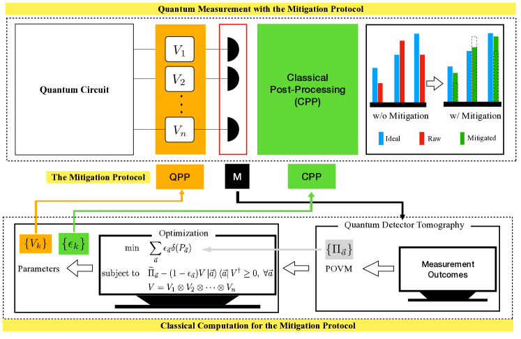
Figure 1: The mitigation protocol applies local unitaries $V_{1}\otimes V_{2}\otimes\cdots\otimes V_{n}$ before detection events, see Eq. (5), to revert to a product POVM element, and then the classical post-processing that realizes the reciprocal relation in Eq. (8). In the quantum part, local unitaries are additionally applied after all. To find optimal local unitaries and classical post-processing, quantum detector tomography is performed to verify POVM elements so that optimal parameters are identified.

The mitigation protocol. Let us begin by describing positive-operator-valued-measure (POVM) elements in a realistic scenario. In a noise-free case, a measurement may be performed in the computational basis: for a measurement outcome $\vec{a}=a_{1}a_{2}\cdots a_{n}$ where $a_{i}\in\{0,1\}$, a measurement operator is denoted by, $|\vec{a}\rangle\langle\vec{a}|:=|a_{1}\rangle\langle a_{1}|\otimes\cdots\otimes|a_{n}\rangle\langle a_{n}|$. For an $n$-qubit state $\rho$, the statistics is given by,

$$p_{0}(\vec{a})=\mathrm{tr}[\rho|\vec{a}\rangle\langle\vec{a}|].$$ (1)

For a noisy measurement, let $\Pi_{a_{i}}$ for $1,\cdots,n$ denote a POVM element of an individual qubit so that $n$-qubit measurements may be given by

$$\Pi_{\vec{a}}=\Pi_{a_{1}}\otimes\cdots\otimes\Pi_{a_{n}}.$$ (2)

They fulfill the completeness condition $\sum_{\vec{a}}\Pi_{\vec{a}}=I$. A measurement containing crosstalk noise can be characterized by POVM elements that cannot be factorized in a product form, Sarovar et al. (2020),

$$\Pi_{\vec{a}}\neq\Pi_{a_{1}}\otimes\cdots\otimes\Pi_{a_{n}}.$$ (3)

for all POVM elements of single qubits, $\{\Pi_{a_{i}}\}_{i=1}^{n}$. Note that once a POVM element is identified by quantum detector tomography on multiple qubits, the type of noise contained in detection events may be verified.

A mitigation protocol for measurement readout errors aims to deduce a noise-free statistics shown in Eq. (1) from noisy measurements with POVM elements in Eq. (3). In what follows, provided a POVM element $\Pi_{\vec{a}}$ from quantum tomography, we present a method of mitigating readout errors and then extend to a complete measurement.

The central idea is to exploit a decomposition of a POVM element $\Pi_{\vec{a}}$ as follows,

$$\widetilde{\Pi}_{\vec{a}}:=\frac{{\Pi}_{\vec{a}}}{\mathrm{tr}[{\Pi}_{\vec{a}}]}=(1-\epsilon)~{}V_{\vec{a}}~{}|\vec{a}\rangle\langle\vec{a}|~{}V_{\vec{a}}^{\dagger}+\epsilon P,~{}~{}$$ (4)

where $V_{\vec{a}}=V_{a_{1}}\otimes\cdots\otimes V_{a_{n}}$ is a local unitary transformation with $V_{a_{j}}$ on the $j$th qubit for $j=1,\cdots,n$, a Hermitian operator $P$ of unit trace and some $\epsilon>0$. For convenience, we have used a normalized POVM denoted by $\widetilde{\Pi}_{\vec{a}}$. Since $P$ is not constrained, one can always find a decomposition in Eq. (4) for a POVM element $\Pi_{\vec{a}}$. The decomposition varies depending on the choice of the parameters $\epsilon$ and $P$, see Fig. 2.

The mitigation protocol relies on the parameters in the decomposition in Eq. (4) and works as follows. The first step is to place local unitaries $V_{\vec{a}}$ right before corresponding detectors. We call this step a quantum pre-processing, by which the transformation of a POVM element is realized as follows, see also Fig. 1,

$$\widetilde{\Pi}_{\vec{a}}\mapsto V_{\vec{a}}^{\dagger}~{}\widetilde{\Pi}_{\vec{a}}~{}V_{\vec{a}}=(1-\epsilon)~{}|\vec{a}\rangle\langle\vec{a}|~{}+\epsilon V_{\vec{a}}^{\dagger}PV_{\vec{a}}.$$ (5)

A measurement on an $n$-qubit state provides an outcome $\vec{a}$ with probabilities in the following,

$$p_{e}(\vec{a}) = \mathrm{tr}[\rho V_{\vec{a}}^{\dagger}\Pi_{\vec{a}}V_{\vec{a}}].$$ (6)

Let $q(\vec{a})=\mathrm{tr}[\rho V_{\vec{a}}^{\dagger}PV_{\vec{a}}]$ denote an expectation value of the Hermitian operator $V_{\vec{a}}^{\dagger}PV_{\vec{a}}$ in the decomposition in Eq. (4). From these, it holds that

$$(\mathrm{tr}[\Pi_{\vec{a}}])^{-1}p_{e}(\vec{a})=(1-\epsilon)~{}p_{0}(\vec{a})+\epsilon~{}q(\vec{a}),$$ (7)

where $p_{0}(\vec{a})$ is a noise-free one in Eq. (1), that may be approximated by quantum error mitigation.

Concerning with Eq. (7), we recall that the parameter $\mathrm{tr}[\Pi_{\vec{a}}]$ is immediately known from quantum detector tomography. Thus, the left-hand-side is empirical. The terms in the right-hand-side are hypothetical: in particular, since $P$ is not positive in general, the value $q(\vec{a})$ cannot be obtained directly. For practical purposes, let us fix $q(\vec{a})$ by a constant $\eta\in[0,1]$ in Eq. (7) and later discuss how to choose the parameter.

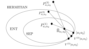
Figure 2: A POVM element in Eq. (4) for two qubits can be decomposed as a convex combination of product states and an operator $P$ of unit-trace. The choice of local unitaries $V$ is directly connected to the properties of operator $P$, that can be separable, entangled, or non-positive. Note that depending on a choice of $P$, the fraction $\epsilon$ varies and determines a resulting error rate after the proposed mitigation protocol, see Eq. (11).

Having obtained a statistics $p_{e}(\vec{a})$ by the aforementioned quantum pre-processing, the next step is to apply a reciprocal relation with a constant $\eta\in[0,1]$ to measurement outcomes:

$$p_{e}(\vec{a})\mapsto p_{0}^{(\eta)}(\vec{a})=\frac{1}{1-\epsilon}\big{(}(\mathrm{tr}\Pi_{\vec{a}})^{-1}p_{e}(\vec{a})-\epsilon~{}\eta\big{)},$$ (8)

where $p_{0}^{(\eta)}(\vec{a})$ denotes an approximation to the noise-free probability with a choice of $\eta$. The error is estimated as,

$$\mathrm{err}(\epsilon,\eta):=|p_{0}(\vec{a})-p_{0}^{(\eta)}(\vec{a})|=\frac{\epsilon|q(\vec{a})-\eta|}{1-\epsilon}.$$ (9)

It is clear that the error above depends on the parameter $\epsilon$ from the decomposition in Eq. (4) and a choice of $\eta$ replacing $q(\vec{a})$ in Eq. (7), both of which are in a percent level. After all, the error is $O(\epsilon|q(\vec{a})-\eta|)$ which is found in a percent level. We also remark that the mitigation protocol is valid on $n$ qubits in general.

It is desired to find the parameters $\eta$ and $\epsilon$ used in the classical post-processing such that the error bound in Eq. (9) is minimized. After some calculations, it may be found that the bound depends on the spectral gap of the operator $P$ in Eq. (4). From this, it may be suggested to choose the parameter $\eta$ as an average,

$$\eta:=q_{c}=\frac{1}{2}{(b_{+}(P)+b_{-}(P))}$$ (10)

$$\mathrm{where}~{}~{}b_{+}(P)=\max_{\rho}\mathrm{tr}[\rho P]~{}~{}\mathrm{and}~{}~{}b_{-}(P)=\min_{\rho}\mathrm{tr}[\rho P].$$

With the parameters above, the bound is given as follows,

$$\mathrm{err}(\epsilon,q_{c})\leq\frac{\epsilon\delta(P)}{(1-\epsilon)}$$ (11)

where $\delta(P)=(b_{+}(P)-b_{-}(P))/2$.

It is then left to construct a decomposition of a POVM element shown in Eq. (4), to find optimal parameters $\epsilon$ and $P$. The difficulty to find an optimal decomposition in Eq. (4) lies in the fact that a unit operator $P$ is not constrained. For convenience, let us fix $P\geq 0$ so that suboptimal parameters can be obtained as follows:

$$\min \epsilon~{}\delta(P)$$ (12)

$$\mathrm{subject~{}to} \widetilde{\Pi}_{\vec{a}}-(1-\epsilon)V|\vec{a}\rangle\langle\vec{a}|V^{\dagger}\geq 0.$$

$$V=V_{1}\otimes V_{2}\otimes\cdots\otimes V_{n}.$$

We recall that the error is within a range in Eq. (11).

The mitigation protocol contains advantages as follows. First, the protocol applies single-qubit gates only in the quantum pre-processing, that has an error rate $0.1\%$ in NISQ systems such as superconducting qubits and trapped ions, whereas a measurement readout error is about a few percents. Thus, the protocol is feasible and cost effective. Second, we emphasize that the mitigation protocol deals with crosstalk errors in a quantum measurement.

We now visit two- and three-qubit measurements in Rigetti and IBMQ with the mitigation protocol, through the cloud-based quantum computing services. The detailed analysis is shown in Appendices I and II.

Example 1 (Rigetti Aspen-8). Quantum detector tomography for qubits labelled $0$ and $1$ in the Rigetti Aspen-8 processor has been performed on Jan. $16$ in 2021. Although readout errors are small for single qubits, they significantly increase for two qubits. It is found that the POVM giving outcome $00$ contains detection crosstalk. The error rate for two-qubit measurements is given by $26\%$, which may be reduced up to $11\%$ by the mitigation protocol.

Example 2 (IBMQ Yorktown). Quantum detector tomography for three qubits labelled $0$, $1$, and $2$ in IBMQ Yorktown has been performed on Nov. 13 2020. It is observed that the POVM element giving outcome $000$ contains an error rate about $15\%$, which may be reduced up to $8\%$ by the mitigation protocol. Crosstalk is also detected in the POVM element.

It is straightforward to extend the mitigation protocol to a complete measurement. One can start by constructing a decomposition of POVM elements: for all $\vec{a}$,

$$\widetilde{\Pi}_{\vec{a}}=(1-\epsilon_{\vec{a}})~{}V~{}|\vec{a}\rangle\langle\vec{a}|~{}V^{\dagger}+\epsilon_{\vec{a}}P_{\vec{a}},~{}~{}$$ (13)

with $\epsilon_{\vec{a}}>0$. Local unitaries $V=\otimes_{i=1}^{n}V_{i}$ are applied such that they are independent to outcomes $\vec{a}$. In this case, one may consider an optimization as follows,

$$\min \sum_{\vec{a}}\epsilon_{\vec{a}}~{}\delta(P_{\vec{a}})$$ (14)

$$\mathrm{subject~{}to} \widetilde{\Pi}_{\vec{a}}-(1-\epsilon_{\vec{a}})V|\vec{a}\rangle\langle\vec{a}|V^{\dagger}\geq 0,~{}~{}\forall\vec{a}$$

$$V=V_{1}\otimes V_{2}\otimes\cdots\otimes V_{n}.$$

Placing local unitaries $V$ obtained above before a measurement, one applies the classical post-processing with the measurement outcomes $\vec{a}$, see Eq. (8).

Application to Entanglement Detection. We in particular apply the mitigation protocol to the task of certifying entangled states. As entanglement is a general resource in quantum information processing, it is crucial to detect its presence for having quantum advantages Horodecki et al. (2009). Entanglement generation is also a key element for a circuit to be useful, see e.g., parameterized quantum circuits Sim et al. (2019); Du et al. (2020); Grant et al. (2018); Toyama et al. (2013) in variational algorithms. Clearly, all entangled states are useful in quantum information processing Horodecki et al. (1999); Masanes (2006). Once the mitigation protocol can detect a larger set of circuits which can generate entangled states, it may be envisaged that the protocol can be also used to improve circuit-based tasks in general, such as variational quantum algorithms.

Entanglement witnesses (EWs) are the most feasible tool to detect entangled states. These are Hermitian operators being non-negative for all separable states and negative for some entangled ones Terhal (2000); Lewenstein et al. (2000); Gühne and Tóth (2009); Chruściński and Sarbicki (2014). Recently, the framework of EW 2.0 has been presented Bae et al. (2020), where all standard EWs can be upgraded to detect a twice larger set of entangled states. The framework of EW 2.0 considers a non-negative and unit trace operator $\widetilde{W}$ constructed by an EW such that two EWs can be realized simultaneously,

$$B_{L}\leq\mathrm{tr}[\widetilde{W}\sigma_{\mathrm{sep}}]\leq B_{U}~{}~{}~{}\forall\sigma_{\mathrm{sep}}\in\mathrm{SEP}$$ (15)

where $\mathrm{SEP}$ denotes the set of all separable states and $B_{L}$ ($B_{U}$) is a lower (upper) bound satisfied by all separable states. The range $[B_{L},B_{U}]$ is called the separability window of $\widetilde{W}$. Each of the inequalities correspond to an EW, and thus violation of either bound concludes entangled states.

The goal is to certify entanglement generation by a quantum circuit in a NISQ system. The EW 2.0 in Eq. (61) is equivalently written as follows,

$$\mathrm{tr}[\widetilde{W}\rho]=\mathrm{tr}[|0\rangle\langle 0|^{\otimes 2n}~{}U_{\widetilde{W}}^{\dagger}(\rho\otimes I_{n})U_{\widetilde{W}}]:=p_{e}(\vec{0}).~{}~{}$$ (16)

Let us explain the equation above. The $2n$-qubit unitary transformation $U_{\widetilde{W}}$ prepares an EW,

$$\widetilde{W}=\mathrm{tr}_{n}U_{\widetilde{W}}|0\rangle\langle 0|^{\otimes 2n}U_{\widetilde{W}}^{\dagger}$$ (17)

where $\mathrm{tr}_{n}$ denotes tracing over $n$ qubits. I.e., an operator $\widetilde{W}$ is prepared by quantum circuit $U_{\widetilde{W}}$ to a fixed state $|0\rangle^{\otimes 2n}$ and tracing out the second half. Exploiting the relation above, one can also relax the assumption of qubit allocations Seong and Bae (2021).

After all, the expectation in Eq. (16) corresponds to the probability of obtaining an $n$-bit outcome sequence $\vec{0}$ in the first half, denoted by $p_{e}({\vec{0}})$. Entangled states are certified if it is found $p_{e}(\vec{0})\notin[B_{L},B_{U}]$. Note that the probability $p_{e}(\vec{0})$ is obtained from a single POVM element $\widetilde{\Pi}_{\vec{0}}$ that gives outcomes $\vec{0}$. This means it suffices to mitigate noise appearing in the POVM element. After a mitigation protocol is applied, an entanglement-generating circuit is certified if $p_{0}^{(\eta)}(\vec{0})\notin[B_{L},B_{U}]$. By the mitigation protocol, one may detect a larger set of entangled states.

Let us consider an entangled state which is not detected by noisy measurement yet such that

$$p_{e}(\vec{0})>B_{L}+\kappa~{}~{}~{}\mathrm{or}~{}~{}~{}p_{e}(\vec{0})<B_{U}-\kappa$$

for some $\kappa>0$. The entangled state may be detected after error mitigation, i.e., one may have $p_{0}^{(\eta)}(\vec{0})<B_{L}$ or $p_{0}^{(\eta)}(\vec{0})>B_{U}$. This can happen whenever the parameter $\eta$ in Eq. (10) is chosen such that

$$\frac{1}{\epsilon}(cB_{L}+(\mathrm{tr}\Pi_{\vec{0}})^{-1}\kappa)<\eta<\frac{1}{\epsilon}(cB_{U}-(\mathrm{tr}\Pi_{\vec{0}})^{-1}\kappa)~{}~{}~{}$$ (18)

where $c=\big{(}(\mathrm{tr}\Pi_{\vec{0}})^{-1}-(1-\epsilon)\big{)}$.

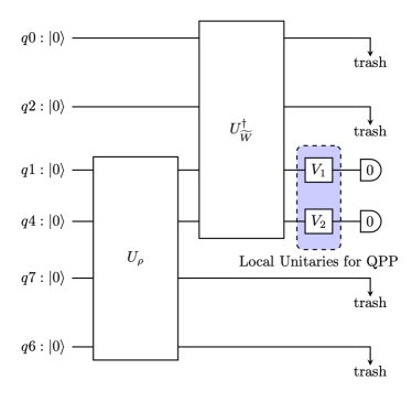
Figure 3: A scheme for certifying two-qubit entangled states is shown. An arbitrary two-qubit state $\rho$ is prepared by a circuit $U_{\rho}$ for four qubits where two ancilla qubits are used. An EW 2.0 operator $\widetilde{W}$ for two-qubit states can be realized by $U_{\widetilde{W}}^{\dagger}$, see Eq. (16). Then, the probability of getting outcome $00$ corresponds to $p_{e}(00)$ in Eq. (16). When two detectors in $q_{1}$ and $q_{4}$ contain crosstalk noise, a quantum pre-processing (QPP) applies by local unitaries right before a measurement.

We realize the mitigation protocol in IBMQ Sydney on Mar. 25 2021, see Appendix IV for details. Two qubits labelled $1$ and $4$ in IBMQ Sydney are considered and measured for detecting entangled states, see Fig. 3. From quantum detector tomography, the error rate in a two-qubit readout is found $12.13\%$ containing crosstalk noise. It is reduced up to $12.01\%$ by implementing a quantum pre-processing and also up to $7\%$ by a classical post-processing.

In the following, we apply the protocol to the certification of entanglement-generating circuits via the framework of EW 2.0. Note that in the cloud-based quantum computing, a circuit design is sent out to the service and measurement outcomes are reported, from which one may conclude entangled states. Circuits to prepare noisy entangled states in the following are considered,

$$\rho_{|\psi\rangle}(r)=(1-r)|\psi\rangle\langle\psi|+\frac{r}{4}I,$$

for $\psi=\phi^{+},\psi^{-}$ and $r=3/8$. In Fig. 3, it is shown that a unitary transformation $U_{\rho}$ such that $\rho=\mathrm{tr}_{q_{6},q_{7}}U_{\rho}|0\rangle\langle 0|^{\otimes 4}U_{\rho}^{\dagger}$ is applied and to be certified if it is an entanglement-generating circuit. The states are entangled for $r<2/3$. The circuits that prepare entangled states above are shown in Appendix IV.

To detect entangled states after the designed circuits are applied, the circuit that prepares an EW 2.0 operator in the following is performed,

$$\widetilde{W}=\frac{1}{4}|\phi^{-}\rangle\langle\phi^{-}|+\frac{1}{4}|\psi^{+}\rangle\langle\psi^{+}|+\frac{1}{2}|\psi^{-}\rangle\langle\psi^{-}|$$ (19)

where $|\psi^{\pm}\rangle=(|01\rangle\pm|10\rangle)/\sqrt{2}$ and $|\phi^{\pm}\rangle=(|00\rangle\pm|11\rangle)/\sqrt{2}$. It holds that for separable states $\sigma_{\mathrm{sep}}$, the lower and upper bounds are given by, see Eq. (61),

$$B_{L}=0.1250~{}~{}\mathrm{and}~{}~{}B_{U}=0.3750$$ (20)

where the lower bound detects $|\phi^{+}\rangle$ and the upper one $|\psi^{-}\rangle$, i.e., $\mathrm{tr}[\widetilde{W}|\phi^{+}\rangle\langle\phi^{+}|]=0$ and $\mathrm{tr}[\widetilde{W}|\psi^{-}\rangle\langle\psi^{-}|]=1/2$. Thus, two EWs are realized via the framework of EW 2.0 in Eq. (19). Note that two EWs are not tight since they can detect entangled states for $r<1/2$.

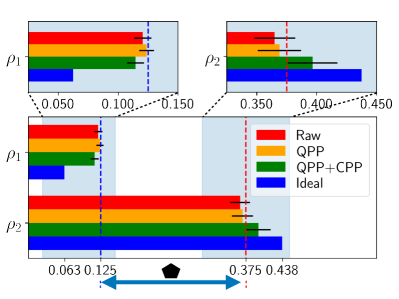
Figure 4: The states $\rho_{1}:=\rho_{\phi^{+}}(3/8)$ and $\rho_{2}:=\rho_{\psi^{-}}(3/8)$ are prepared and entanglement detection is performed in IBMQ Sydney. Note that there are errors in the gates and SPAM. In a noise-free scenario, the entangled state $\rho_{1}$ would have the probability $p(00)=0.0625$, which violates the lower bound $0.1250$ satisfied by all separable states. The entangled state $\rho_{2}$ would have $p(00)=0.4375$ over the upper bound $0.3750$ satisfied by all separable states. The black pentagon denotes the separability window in which no entangled state exist. Then, the raw data (red) are improved by the mitigation protocol (blue). The result only with the quantum pre-processing is denoted in the middle (green), see also Table 1. For each state, the experiment is repeated $15$ times and the standard deviation is around $1\%$.

State	$p_{0}(00)$	$p_{e}(00)$	QPP	$~{}p_{0}^{(\eta)}(00)$
$\rho_{\phi^{+}}(3/8)~{}$	0.0625	0.1206	0.1238	0.1145
$\rho_{\phi^{+}}(1/2)~{}$	$B_{L}$	0.1625	0.1635	0.1602
$\rho_{\psi^{-}}(1/2)~{}$	$B_{U}$	0.3187	0.3286	0.3501
$\rho_{\psi^{-}}(3/8)~{}$	0.4375	0.3649	0.3953	0.3967

Table 1: A comparison among ideal, experimental and post-processed $p(00)$. The results in the column QPP are obtained by applying the quantum pre-processing only. It is shown that the mitigation protocol improves the certification of entanglement-generating circuits, see Fig. 4.

The results of entanglement-generation circuits in IBMQ is summarized in Table 1 and also Fig. 4. The circuits in detail are also shown in Appendix IV. The sources of noise in the demonstration are i) state preparation and measurement (SPAM) and ii) single- and two-qubit gates. Then, as for an entangled state $\rho_{\psi^{-}}(3/8)$, the measurement outcomes show $0.3649<B_{U}$ and thus cannot conclude an entangled state. By the quantum pre-processing with local unitary transformations on qubits $q_{1}$ and $q_{4}$, see Fig. 3, the statistics is improved to $0.3953>B_{U}$, that concludes an entangled state, and then by the classical post-processing, up to $0.3967$ which makes entanglement-generation even clearer. The experiment is repeated $15$ times and the statistical fluctuation is found about $1\%$.

Similarly for the state $\rho_{\phi^{+}}(3/8)$, the measurement outcomes show $0.1206<B_{L}$ which is then updated to $0.1238$ by the quantum pre-processing and then to $0.1145$ by the classical post-processing. In this case, it may be noticed that SPAM errors are dominant. Then, the mitigation protocol makes the certification of entanglement-generating circuits even clearer.

Conclusion. In conclusion, we have shown that measurement readout errors on multiple qubits can be mitigated up to a percent level. The mitigation protocol is presented to deal with both individual and crosstalk errors. The protocol is also feasible with current technologies that can realize single-qubit gates with high precision: hence, the protocol can be applied to measurement errors in the NISQ systems. In particular, measurement error mitigation can be exploited to improve hybrid quantum-classical algorithms that rely on repeated applications of measurements on multiple qubits meanwhile, e.g., McClean et al. (2016); Endo et al. (2021); Cerezo et al. (2020); Bharti et al. (2021). We also envisage that the protocol of measurement error mitigation would be concatenated to quantum error-correcting codes that deal with all types of noise appearing in a quantum circuit.

We have in particular considered two- and three-qubit measurements in Rigetti and IBMQ. Crosstalk errors in a measurement of multiple qubits in the devices are shown and the protocol of measurement error mitigation is realized. Then, the mitigation protocol is applied to the certification of entanglement-generating circuits and enhances the capability of entanglement detection: a larger set of entangled states can be efficiently detected. Our results can be applied to the hybrid quantum-classical algorithms where measurements are repeatedly performed, such as variational quantum algorithms and certification of the capabilities of parameterized quantum circuits in practice Sim et al. (2019); Du et al. (2020); Grant et al. (2018); Toyama et al. (2013).

From a fundamental point of view, our results shed new light on the approaches to dealing with crosstalk errors in quantum systems. Technically, it is shown that detection crosstalk can be tackled by analyzing decompositions of POVM elements in Eq. (4). In future directions, it would be interesting to investigate correlations existing in POVM elements and classify crosstalk errors. For instance, it is worth mentioning that those POVM elements we have considered in Rigetti and IBMQ are found to be separable, i.e., non-negative under the partial transpose. Finally, it would be interesting to seek the possibility of circumventing quantum detector tomography that may cost significant resources as the number of qubits increases.

Appendix

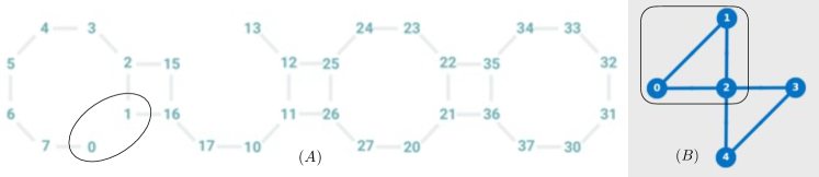
Figure 5: (A) Quantum detector tomography for qubits labelled $0$ and $1$ in the Rigetti Aspen-8 processor is performed, see Eq. (25). Gray lines show connectivity of qubits. (B) The qubit array of IBMQ Yorktown is shown. Quantum detector tomography is performed on qubits labelled by $0$, $1$, and $2$, all of which are connected one another.

Appendix I: The Rigetti Aspen-8 processor

We have performed quantum detector tomography for qubits labelled $0$ and $1$ in the Rigetti Aspen-8 processor, see Fig. 5, on Jan. $16$ in 2021. The Aspen-8 processor is composed of $33$ qubits. The error rate of single-qubit gates is around $0.01\%$, whereas those of two-qubit gates and a measurement are about $5$-$8\%$. Quantum detector tomography is performed by preparation and measurement of mutually unbiased bases. Then, the POVM element giving outcome $00$ is found as follows

$$\widetilde{\Pi}_{00}=\left(\begin{array}[]{cccc}0.7395&0.0060-0.0179i&0.0391-0.0189i&0.0082-0.0096i\\ 0.0060+0.0179i&0.1993&-0.0109+0.0434i&-0.0082-0.0241i\\ 0.0391+0.0189i&-0.0109-0.0434i&0.0473&-0.0089+0.0003i\\ 0.0082+0.0096i&-0.0082+0.0241i&-0.0089-0.0003i&0.0138\end{array}\right)$$ (25)

with $\mathrm{tr}[\Pi_{00}]=0.8742$. It is found that the POVM element cannot be factorized and thus contains detection crosstalk. The error rate for two-qubit measurements is given by $26\%$.

One can apply the mitigation protocol proposed in the main text by finding a decomposition of the POVM. The error rate may be reduced up to $11\%$. To be specific, the quantum pre-processing can be performed by local unitaries in the following,

$$V_{1} = \left(\begin{array}[]{cccc}0.9930+0.0000i&-0.0592-0.1023i\\ 0.0952+0.0700i&-0.1075+0.9872i\end{array}\right)$$ (28)

$$V_{2} = \left(\begin{array}[]{cccc}0.9994+0.0000i&-0.0019-0.0357i\\ 0.0282+0.0221i&-0.5745+0.8177i\end{array}\right).$$ (31)

For the classical post-processing, the parameters for the mitigation protocol may be chosen as follows, $\epsilon=0.2940$ and $\delta(P)=0.3683$.

Appendix II: IBMQ Yorktown

We have performed quantum detector tomography for three qubits labelled $0$, $1$, and $2$ in IBMQ Yorktown on Nov. 13 2020. The qubits are in fact connected with each other, see Fig. 5. The POVM element giving outcome $000$ is found by

$$\Pi_{000}=\left(\begin{array}[]{cccccccc}.849&-.001-.01i&-.008i&.004+.002i&.001i&-.004&-.008+.01i&.003+.001i\\ *&.036&.001-.002i&-0.001i&-.001-.002i&.001-.001i&.009+.001i&.001-.001i\\ *&*&.104&-.001+.001i&.006+.005i&.006+.001i&.007i&.005+.001i\\ *&*&*&.0037&.003i&-.001+.001i&.001i&0\\ *&*&*&*&.281&.001+.007i&.004+.001i&-.006+.003i\\ *&*&*&*&*&.012&-.008+.003i&.001+.001i\\ *&*&*&*&*&*&.031&.001-.002i\\ *&*&*&*&*&*&*&.001\end{array}\right)$$ (40)

with $\mathrm{tr}[\Pi_{000}]=1.32$. Note also that $\Pi_{000}=\Pi_{000}^{\dagger}$. From above, it is observed that the POVM element giving outcome $000$ contains an error rate about $15\%$.

The mitigation protocol can reduce the error rate up to $8\%$. Specifically, one can choose the parameters $\epsilon=0.463$ and $\delta(P)=0.231$. It is note worthy that, with the parameters, the operator $P\geq 0$ in the decomposition of the POVM element turns out to be entangled. In particular, it is found that the operator is entangled, i.e., negative after the partial transpose in the bipartite splitting $1:02$ and $2:01$.

Appendix III: Entanglement witness 2.0 with noisy detectors

A standard EW corresponds to a Hermitian operator $W=W^{\dagger}$ such that $\mathrm{tr}[W\sigma_{\mathrm{sep}}]\geq 0$ for all separable states $\sigma_{\mathrm{sep}}$ but $\mathrm{tr}[W\rho]\geq 0$ for some entangled states $\rho$. In EW 2.0, two EWs can be can be encapsulated into lower and upper bounds, respectively, of a non-negative operator $\widetilde{W}$ as follows,

$$\forall\sigma_{\mathrm{sep}},~{}~{}B_{L}\leq\mathrm{tr}[\widetilde{W}\sigma_{\mathrm{sep}}]\leq B_{U}.$$ (41)

Each of the inequalities above is characterized by a standard EW, and entangled states are detected by observing violations of the inequalities. Thus, an EW 2.0 operator can detect a twice larger set of entangled states. Note that the gap of the bounds is called the separability window, denoted by $\Delta=[B_{L},B_{U}]$.

The expectation value in Eq. (41) can be rewritten as

$$\mathrm{tr}[\widetilde{W}\rho]=\mathrm{tr}[|0\rangle\langle 0|^{\otimes 2n}~{}U_{\widetilde{W}}^{\dagger}(\rho\otimes I_{n})U_{\widetilde{W}}]:=p_{e}(\vec{0}),$$

where the EW 2.0 operator can be derived as

$$\widetilde{W}=\mathrm{tr}_{n}U_{\widetilde{W}}|0\rangle\langle 0|^{\otimes 2n}U_{\widetilde{W}}^{\dagger}.$$

This shows that a measurement outcome $\vec{0}$ suffices to certify entanglement-generating circuits.

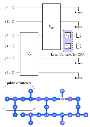
Figure 6: The connectivity of IBMQ Sydney is shown. Qubits labelled by $0,1,2,4,6,7$ are used in the verification of entanglement-generating circuits. The qubits are denoted by $q_{0},\cdots,q_{7}$ in the circuit. A circuit $U_{\rho}$ generates an entangled state $\rho$, and then $U_{\widetilde{W}}^{\dagger}$ that prepares an EW 2.0 operator $\widetilde{W}$ certifies entanglement generation. Entangled states generated in qubits $4$ and $7$ are certified, to which the measurement mitigation protocol is applied. Two local unitaries $V_{1}\otimes V_{2}$ are applied as the quantum pre-processing (QPP). The circuits for state preparation and the EW 2.0 operator in detail are shown in Figs. 7 and 8.

When a measurement is noisy, the inequalities may be rewritten as,

$$B_{L}\leq p_{e}(\vec{0})\leq B_{U}.$$ (42)

Note that since noise exists in a measurement, the bounds are not as tight as the noise-free ones. The mitigation protocol transforms the probability as,

$$p_{0}^{(\eta)} = \frac{(\mathrm{tr}\Pi_{\vec{0}})^{-1}}{1-\epsilon}p_{e}(\vec{0})-\frac{\epsilon}{1-\epsilon}\eta,$$

for which the bounds are rewritten as

$$B_{L}^{(\eta)}\leq p_{0}^{(\eta)}(\vec{0})\leq B_{U}^{(\eta)}$$ (43)

where

$$B_{L}^{(\eta)} = \frac{(\mathrm{tr}\Pi_{\vec{0}})^{-1}}{1-\epsilon}B_{L}-\frac{\epsilon}{1-\epsilon}\eta$$

$$B_{U}^{(\eta)} = \frac{(\mathrm{tr}\Pi_{\vec{0}})^{-1}}{1-\epsilon}B_{U}-\frac{\epsilon}{1-\epsilon}\eta.$$

Note that the inequality in Eq. (43) may be tighter than the other in Eq. (42) so that a larger set of entangled states can be detected.

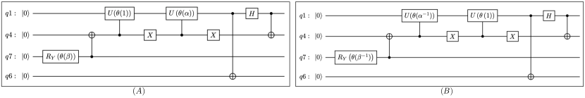
Figure 7: Circuits that prepare (A) $\rho_{\phi^{+}}(p)$ and (B) $\rho_{\psi^{-}}(p)$ in Eq. (59) are shown with the parameters in Eq. (60).

Appendix IV: The mitigation protocol in IBMQ Sydney

Quantum detector tomography for qubits labelled by $q_{1}$ and $q_{4}$ in IBMQ Sydney are performed on Mar. 25 2021, see Fig. 6. The POVM element giving outcome $00$ is obtained as follows

$$\Pi_{00}=\left(\begin{array}[]{cccc}0.8787&-0.0026-0.0011i&-0.0007-0.0031i&-0.0028-0.0045i\\ -0.0026+0.0011i&0.0090&0.0004-0.0002i&0.0002+0.0010i\\ -0.0007+0.0031i&0.0004+0.0002i&0.0366&0.0007-0.0012i\\ -0.0028+0.0045i&0.0002-0.0010i&0.0007+0.0012i&0.0209\end{array}\right)$$ (48)

Note that one has $\mathrm{tr}{\Pi_{00}|00\rangle\langle 00|}=0.8787$, from which the error rate is $12.13\%$. Note also that $\mathrm{tr}{\Pi_{00}}=0.9452$.

The mitigation protocol is the implemented with the parameters $\epsilon=0.0740$, $\delta=0.2597$ ($b_{+}=0.5308$ and $b_{-}=0.0104$) and $\eta=0.2711$. These parameters find a decomposition of the POVM element and also local unitary transformations to be applied in the quantum pre-processing for qubits $q1$ and $q4$:

$$V_{1} = \left(\begin{array}[]{cccc}1.0000+0.0000i&0.0018+0.0006i\\ -0.0015-0.0011i&0.5774+0.8165i\end{array}\right)$$

$$V_{4} = \left(\begin{array}[]{cccc}0.9999+0.0000i&-0.0154-0.0054i\\ 0.0040+0.0159i&-0.0910+0.9957i\end{array}\right).$$ (53)

After applications of $V_{1}$ and $V_{4}$ to the qubits as a quantum pre-processing, we have performed quantum detector tomography that shows POVM elements in the following, see Fig. 6,

$$\Pi_{00}^{(QPP)}=\left(\begin{array}[]{cccc}0.8799&0.0046-0.0105i&-0.0043-0.0032i&0.0019+0.0022i\\ 0.0046+0.0105i&0.0129&0.0059-0.0009i&-0.0003\\ -0.0043+0.0032i&0.0059+0.0009i&0.0448&-0.0036+0.0007i\\ 0.0019-0.0022i&-0.0003&-0.0036-0.0007i&0.0259\end{array}\right).$$ (58)

From the above, it is found that $\mathrm{tr}{\Pi_{00}^{(QPP)}|00\rangle\langle 00|}=0.8799$. This shows the error rate is reduced to $12.01\%$ only by the quantum processing with local unitaries $V_{1}$ and $V_{2}$. This may be reduced up to $7\%$ eventually after the classical post-processing.

Then, entanglement generation on the qubits $q_{1}$ and $q_{4}$ can be detected as follows. As it is shown in Fig. 6, an entangled state is generated by a circuit $U_{\rho}$ to an input state $|0\rangle^{\otimes n}$ and entanglement generation by the circuit is certified by another circuit $U_{\widetilde{W}}^{\dagger}$ that prepares an EW 2.0 operator $\widetilde{W}$.

State	$p_{0}(00)$	$p_{e}(00)$ ($\sigma$)	$p_{0}^{(\eta)}(00)$ ($\sigma$)
$\rho_{\phi^{+}}(3/8)~{}$	0.0625	0.1206 (0.0072)	0.1161 (0.0082)
$\rho_{\phi^{+}}(1/2)~{}$	$B_{L}$	0.1625 (0.0086)	0.1640 (0.0099)
$\rho_{\psi^{-}}(1/2)~{}$	$B_{U}$	0.3187 (0.0107)	0.3425 (0.0123)
$\rho_{\psi^{-}}(3/8)~{}$	0.4375	0.3649 (0.0171)	0.3953 (0.0196)

Table 2: The probabilities of obtaining outcomes $00$ are compared when the quantum pre-processing is lacking, i.e., $V=I\otimes I$. States are shown in the first column, see Eq. (59), and the ideal probabilities are collected in the second column. In the third column, probabilities without error mitigation are shown. These are improved by the mitigation protocol in the fourth column. The experiment is repeated $15$ times and the standard deviation ($\sigma$) is around $1\%$.

In the proof-of-principle demonstration, the following states are considered

$$\rho_{\psi}=(1-p)|\psi\rangle\langle\psi|+\frac{p}{4}I$$ (59)

for $\psi=\phi^{+},\psi^{-}$. To construct a circuit to prepare the states, let $R_{Y}^{(j)}(\theta)$ denote a counterclockwise rotation about the $y$-axis by an angle $\theta$ for a state of the $j$-th qubit. We also write by $C_{U}^{(j,k)}$ a controlled-$U$ gate on the $j$-th and the $k$-th qubits where the latter one is a target qubit. Then, the circuits for preparing states in the above are constructed as follows

$$U_{\phi^{+}}(p) = C_{X}^{(1,4)}H^{(0)}C_{X}^{(1,6)}X^{(4)}C_{U}^{(4,1)}(\alpha)X^{(4)}C_{U}^{(4,1)}(\frac{\pi}{2})\times$$

$$C_{X}^{(7,4)}R_{Y}^{(7)}(\theta(\beta))$$

$$U_{\psi^{-}}(p) = C_{X}^{(1,4)}H^{(1)}C_{X}^{(1,6)}X^{(4)}C_{U}^{(4,1)}(\frac{\pi}{2})X^{(4)}\times$$

$$C_{U}^{(4,1)}(\alpha^{-1})C_{X}^{(7,4)}R_{Y}^{(7)}{\theta(\beta^{-1})}.$$

where

$$\alpha=\frac{1-p}{1+3p},~{}\beta=\frac{1-p}{1+p},~{}\mathrm{and}~{}\theta(p)=2\arctan(\sqrt{p}).~{}~{}~{}~{}~{}$$ (60)

The circuits are also shown in Fig. 7.

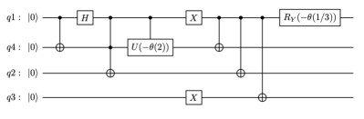
Figure 8: A circuit that prepares $\widetilde{W}$ in Eq. (61) is shown.

State	$p_{0}(00)$	$p_{e}(00)$ ($\sigma$)	$p_{0}^{(\eta)}(00)$ ($\sigma$)
$\rho_{\phi^{+}}(3/8)~{}$	0.0625	0.1238 (0.0061)	0.1145 (0.0071)
$\rho_{\phi^{+}}(1/2)~{}$	$B_{L}$	0.1635 (0.0086)	0.1602 (0.0099)
$\rho_{\psi^{-}}(1/2)~{}$	$B_{U}$	0.3286 (0.0123)	0.3501 (0.0141)
$\rho_{\psi^{-}}(3/8)~{}$	0.4375	0.3690 (0.0180)	0.3967 (0.0207)

Table 3: The probabilities of obtaining outcomes $00$ are compared when the quantum pre-processing is applied, see Eq. (53). In the third column, probabilities obtained after the quantum pre-processing are shown. These are improved by the mitigation protocol in the fourth column. The experiment is repeated $15$ times and the standard deviation ($\sigma$) is around $1\%$. The data may be compared with Table 2.

For the states in Eq. (59), an EW 2.0 operator can be constructed as follows,

$$\widetilde{W}=\frac{1}{4}|\phi^{-}\rangle\langle\phi^{-}|+\frac{1}{4}|\psi^{+}\rangle\langle\psi^{+}|+\frac{1}{2}|\psi^{-}\rangle\langle\psi^{-}|,$$ (61)

which has lower and upper bounds

$$B_{L}=0.125,~{}~{}\mathrm{and}~{}~{}B_{U}=0.375,$$

respectively, satisfied by all separable states. The EW 2.0 operator can be constructed by a circuit follows,

$$U^{\dagger}_{\widetilde{W}} = R_{Y}^{(1)}(-\frac{\pi}{3})C_{X}^{(1,3)}C_{X}^{(1,2)}C_{X}^{(1,4)}X^{(1)}X^{(3)}\times$$

$$C_{U}^{(1,4)}(-\theta(2))CC_{X}^{(1,4,2)}H^{(1)}C_{X}^{(1,4)}.$$

where

$$CC_{X}^{(1,4,2)}=$$

$$|0\rangle\langle 0|^{(1)}\otimes|0\rangle\langle 0|^{(4)}\otimes I^{(2)}+|1\rangle\langle 1|^{(1)}\otimes|1\rangle\langle 1|^{(4)}\otimes X^{(2)}.$$

The circuit is also shown in Fig. 8.

The proof-of-principle demonstration has been performed on Mar. 25 2021. Four states $\rho_{\psi}(3/8)$ and $\rho_{\psi}(4/8)$ where $\psi=\phi^{+},\psi^{-}$ are considered. For each state, the experiment performs a measurement with $8192$ shots and repeated $15$ times. The standard deviation is shown around $1\%$. The results are collected in Tables 2 and 3.

References

- Shor (1995) P. W. Shor, Phys. Rev. A 52, R2493 (1995).
- Gottesman (1997) D. Gottesman, PhD Thesis (1997).
- Kempe (2007) J. Kempe, “Approaches to quantum error correction,” in Quantum Decoherence: PoincaréSeminar 2005, edited by B. Duplantier, J.-M. Raimond, and V. Rivasseau (Birkhäuser Basel, Basel, 2007) pp. 85–123.
- Preskill (2018) J. Preskill, Quantum 2, 79 (2018).
- McClean et al. (2016) J. R. McClean, J. Romero, R. Babbush, and A. Aspuru-Guzik, New Journal of Physics, 18, 023023 (2016).
- Endo et al. (2021) S. Endo, Z. Cai, S. C. Benjamin, and X. Yuan, Journal of the Physical Society of Japan, Journal of the Physical Society of Japan 90, 032001 (2021).
- Cerezo et al. (2020) M. Cerezo, A. Arrasmith, R. Babbush, S. C. Benjamin, S. Endo, K. Fujii, J. R. McClean, K. Mitarai, X. Yuan, L. Cincio, and P. J. Coles, arXiv:2012.09265 (2020).
- Bharti et al. (2021) K. Bharti, A. Cervera-Lierta, T. H. Kyaw, T. Haug, S. Alperin-Lea, A. Anand, M. Degroote, H. Heimonen, J. S. Kottmann, T. Menke, W.-K. Mok, S. Sim, L.-C. Kwek, and A. Aspuru-Guzik, arXiv:2021.08448 (2021).
- Endo et al. (2018) S. Endo, S. C. Benjamin, and Y. Li, Phys. Rev. X 8, 031027 (2018).
- Temme et al. (2017) K. Temme, S. Bravyi, and J. M. Gambetta, Phys. Rev. Lett. 119, 180509 (2017).
- Li and Benjamin (2017) Y. Li and S. C. Benjamin, Phys. Rev. X 7, 021050 (2017).
- McClean et al. (2020) J. R. McClean, Z. Jiang, N. C. Rubin, R. Babbush, and H. Neven, Nature Communications 11, 636 (2020).
- McArdle et al. (2019) S. McArdle, X. Yuan, and S. Benjamin, Phys. Rev. Lett. 122, 180501 (2019).
- Maciejewski et al. (2020) F. B. Maciejewski, Z. Zimborás, and M. Oszmaniec, Quantum 4, 257 (2020).
- Kwon and Bae (2020) H. Kwon and J. Bae, IEEE Transactions on Computers , 1 (2020).
- Chen et al. (2019) Y. Chen, M. Farahzad, S. Yoo, and T.-C. Wei, Phys. Rev. A 100, 052315 (2019).
- Rudinger et al. (2021) K. Rudinger, C. W. Hogle, R. K. Naik, A. Hashim, D. Lobser, D. I. Santiago, M. D. Grace, E. Nielsen, T. Proctor, S. Seritan, S. M. Clark, R. Blume-Kohout, I. Siddiqi, and K. C. Young, arXiv:2103.09890 (2021).
- Sarovar et al. (2020) M. Sarovar, T. Proctor, K. Rudinger, K. Young, E. Nielsen, and R. Blume-Kohout, Quantum 4, 321 (2020).
- Parrado-Rodríguez et al. (2020) P. Parrado-Rodríguez, C. Ryan-Anderson, A. Bermudez, and M. Müller, arXiv:2012.11366 (2020).
- Lienhard et al. (2021) B. Lienhard, A. Vepsäläinen, L. C. G. Govia, C. R. Hoffer, J. Y. Qiu, D. Ristè, M. Ware, D. Kim, R. Winik, A. Melville, B. Niedzielski, J. Yoder, G. J. Ribeill, T. A. Ohki, H. K. Krovi, T. P. Orlando, S. Gustavsson, and W. D. Oliver, Deep Neural Network Discrimination of Multiplexed Superconducting Qubit States, arXiv:2102.12481, to appear in Physical Review Applied (2021).
- Seo and Bae (2021) S. Seo and J. Bae, IEEE Internet Computing , 1 (2021).
- Wang et al. (2021) K. Wang, Y.-A. Chen, and X. Wang, arXiv:2103.13856 (2021).
- Geller (2020) M. R. Geller, Quantum Science and Technology 5, 03LT01 (2020).
- Geller (2021) M. R. Geller, Phys. Rev. Lett. 127, 090502 (2021).
- Maciejewski et al. (2021) F. B. Maciejewski, F. Baccari, Z. Zimborás, and M. Oszmaniec, Quantum 5, 464 (2021).
- Horodecki et al. (2009) R. Horodecki, P. Horodecki, M. Horodecki, and K. Horodecki, Rev. Mod. Phys. 81, 865 (2009).
- Sim et al. (2019) S. Sim, P. D. Johnson, and A. Aspuru-Guzik, Advanced Quantum Technologies 2, 1900070 (2019), https://onlinelibrary.wiley.com/doi/pdf/10.1002/qute.201900070 .
- Du et al. (2020) Y. Du, M.-H. Hsieh, T. Liu, and D. Tao, Phys. Rev. Research 2, 033125 (2020).
- Grant et al. (2018) E. Grant, M. Benedetti, S. Cao, A. Hallam, J. Lockhart, V. Stojevic, A. G. Green, and S. Severini, npj Quantum Information 4, 65 (2018).
- Toyama et al. (2013) F. M. Toyama, W. van Dijk, and Y. Nogami, Quantum Information Processing 12, 1897 (2013).
- Horodecki et al. (1999) P. Horodecki, M. Horodecki, and R. Horodecki, Phys. Rev. Lett. 82, 1056 (1999).
- Masanes (2006) L. Masanes, Phys. Rev. Lett. 96, 150501 (2006).
- Terhal (2000) B. M. Terhal, Physics Letters A 271, 319 (2000).
- Lewenstein et al. (2000) M. Lewenstein, B. Kraus, J. I. Cirac, and P. Horodecki, Phys. Rev. A 62, 052310 (2000).
- Gühne and Tóth (2009) O. Gühne and G. Tóth, Physics Reports 474, 1 (2009).
- Chruściński and Sarbicki (2014) D. Chruściński and G. Sarbicki, Journal of Physics A: Mathematical and Theoretical, 47, 483001 (2014).
- Bae et al. (2020) J. Bae, D. Chruściński, and B. C. Hiesmayr, npj Quantum Information 6, 15 (2020).
- Seong and Bae (2021) J. Seong and J. Bae, , arXiv:2110.10528 (2021).