Local properties of the $t$-$J$ model in a two-pole approximation within COM

Abstract

In this work, we study the $t$-$J$ model using a two-pole approximation within the composite operator method. We choose a basis of two composite operators – the constrained electrons and their spin-fluctuation dressing – and approximate their currents in order to compute the corresponding Green’s functions. We exploit the algebraic constraints obeyed by the basis operators to close a set of self-consistent equations that is numerically solved. This allows to determine the physical parameters of the system such as the spin-spin correlation function and the kinetic energy. Our results are compared to those of an exact numerical method on a finite system to asses their reliability. Indeed, a very good agreement is achieved through a far less numerically demanding and a more versatile procedure. We show that by increasing the hole doping, anti-ferromagnetic correlations are replaced by ferromagnetic ones. The behavior on changing temperature and exchange integral is also studied and reported.

1 Introduction

Strongly correlated systems have undergone extensive study for several decades [1, 2, 3]. For lattice systems, the onsite interaction is the most important one, a feature which is well reflected in the Hubbard model [4, 5, 6]. Despite its seemingly simple structure, the Hubbard model and its extensions and derivations have been very successful in studying strongly correlated systems [7, 8, 9, 10]. In the strong electron-electron repulsion regime, it is possible to derive an effective model from the Hubbard model in which the double-occupancy is discarded according to its extreme energy cost: the so called $t$-$J$ model [11, 12, 13, 14, 15, 16]. The Hubbard and the $t$-$J$ models have been used to theoretically understand and describe so many interesting phenomena such as Mott-Hubbard metal-insulator transition [17], non-Fermi-liquid normal phases and high-temperature superconductivity [18, 19, 20, 21, 22, 23, 24, 25, 26, 27], etc. One feature which is very interesting and still needs to be clarified is the occurrence of a ferro-antiferromagnetic crossover in the $t$-$J$ model [28, 29]. It is quite well-known that, at half filling, the system is in the anti-ferromagnetic (AF) Nï¿œel state. Yet, Nagaoka proved that in the infinite-$U$ regime of the Hubbard model, which corresponds to vanishing exchange integral in the $t$-$J$ model, if we introduce one hole into the system the ground state becomes ferromagnetic (FM) [30, 31, 32]. This idea got generalized in the $t$-$J$ model by so many successive studies which showed transition to FM phase for finite hole dopings [33, 34, 35, 36, 37, 38, 39, 40, 41].

In studying strongly correlated systems, quasi-particles play a crucial role. In the composite operator method (COM), the equation of motion of the operators corresponding to the most relevant quasi-particles, those associated with the emergent elementary excitations in the system, are investigated. Within this method, using the properties of the generalized Green’s functions (GFs) of the quasi-particle operators and their algebraic constraints, a set of self-consistent equations are obtained from which the physical properties can be computed [21, 42, 43, 44, 45, 46]. It’s worth noticing that COM belongs to the large class of operatorial approaches: the Hubbard approximations [4], an early high-order GF approach [47], the projection operator method [48, 49], the works of Mori [50], Rowe [51], and Roth [52], the spectral density approach [53], the works of Barabanov [54], Val’kov [55], and Plakida [56, 57, 58, 59, 60], and the cluster perturbation theory in the Hubbard-operator representation [61].

In this work, we consider a two-pole approximation for the $t$-$J$ model on a two-dimensional lattice and focus on the quasi-particles describing the constrained electrons and their spin-fluctuation dressing. After computing the currents of our basis operators, we apply a generalized mean-field approximation to project them back on the basis. These currents, together with the integrated spectral weights of the basis, can be exploited to get a set of self-consistent equations that allow to compute the relevant GFs. The remaining unknowns can be related to the GFs using the algebraic constraints obeyed by the composite operators. The solutions of these equations reveal the physical properties of the system in different parametric regimes. The quality of the approximation is assessed by comparing our results to those of an exact numerical study. We find a very good agreement while our method is, on one hand, numerically less demanding and, on the other hand, more versatile as it can be generalized to study several different systems and parameter regimes. We show that the system features AF correlations of the Nï¿œel type near half filling, while by increasing the hole doping it develops FM ones. At higher temperatures, both AF and FM correlations are suppressed and the paramagnetic phase is the favored one. Moreover, as expected, higher and higher values of the exchange integral favor AF correlations and higher values of doping are needed for the emergence of FM fluctuations.

The article is organized as follows. In Sec. 2, we introduce the model and the basis operators we have chosen and describe our method. In Sec. 3, we present our numerical results, assess them by comparison to exact numerical ones, and discuss their relevant features. Finally, in Sec. 4, we give our conclusions.

2 Model and Method

The $t$-$J$ Hamiltonian is derived in the strongly correlated regime of the Hubbard model ($t\ll U$) where an exchange integral $J=4t^{2}/U$ emerges [11, 12, 16]. Its explicit form for a two-dimensional lattice is given by

$$\mathcal{H} =-4t\sum_{i}\xi^{\dagger}\left(i\right)\cdot\xi^{\alpha}\left(i\right)-\mu\sum_{i}\nu\left(i\right)$$

$$+\frac{J}{2}\sum_{i}\left[\nu_{k}\left(i\right)\nu_{k}^{\alpha}\left(i\right)-\nu\left(i\right)\nu^{\alpha}\left(i\right)\right],$$ (1)

where $t$, $J$, and $\mu$ are the nearest-neighbor hopping integral, the exchange integral and the chemical potential, respectively. We set $t$ as energy unit. In this model, double occupancy of sites is prohibited, accordingly one has to use the operator $\xi_{\sigma}\left(i\right)=\left(1-n_{\bar{\sigma}}\left(i\right)\right)c_{\sigma}\left(i\right)$, which describes the transition between empty and singly-occupied sites, with $c_{\sigma}\left(i\right)$ being the annihilation operator of an electron with spin $\sigma$ on the site $i$, and $n_{\sigma}\left(i\right)=c_{\sigma}^{\dagger}\left(i\right)c_{\sigma}\left(i\right)$. We use the spinorial notation $\xi^{\dagger}\left(i\right)=\left(\xi_{\uparrow}^{\dagger}\left(i\right),\xi_{\downarrow}^{\dagger}\left(i\right)\right)$ and define (spin) inner product between operators: $\nu\left(i\right)=\xi^{\dagger}\left(i\right)\cdot\xi\left(i\right)=\sum_{\sigma}\xi_{\sigma}^{\dagger}\left(i\right)\xi_{\sigma}\left(i\right)$ and $\nu_{k}\left(i\right)=\xi^{\dagger}\left(i\right)\cdot\sigma_{k}\cdot\xi\left(i\right)$ are the charge and spin density operators on site $i$, respectively, with $\sigma_{k}$ being the Pauli matrices for $k=1,2,3$. Moreover, for every operator $\phi\left(i\right)$, its projection on the nearest neighbor sites ($\delta_{\left\langle ij\right\rangle}$) is given by $\phi^{\alpha}\left(i\right)=\sum_{j}\alpha_{ij}\phi\left(j\right)=\frac{1}{4}\left[\phi\left(i_{x}+1,i_{y}\right)+\phi\left(i_{x}-1,i_{y}\right)+\phi\left(i_{x},i_{y}+1\right)+\phi\left(i_{x},i_{y}-1\right)\right]$, where for a two-dimensional square lattice $\alpha_{ij}=\frac{1}{4}\delta_{\left\langle ij\right\rangle}$. With some straightforward calculations, one can rewrite the Hamiltonian as [62]

$$\mathcal{H}=\sum_{i}\xi^{\dagger}\left(i\right)\cdot\left[-4t\xi^{\alpha}\left(i\right)+J\left(\widetilde{\xi}_{0}\left(i\right)+\widetilde{\xi}_{s}\left(i\right)\right)-\left(\mu+\frac{J}{2}\right)\xi\left(i\right)\right],$$ (2)

where the operators

$$\widetilde{\xi}_{0}\left(i\right)=\frac{1}{2}\left(1-\nu^{\alpha}\left(i\right)\right)\xi\left(i\right),$$ (3)

$$\widetilde{\xi}_{s}\left(i\right)=\frac{1}{2}\nu_{k}^{\alpha}\left(i\right)\sigma_{k}\cdot\xi\left(i\right),$$ (4)

describe constrained electronic transitions dressed by nearest-neighbor charge and spin fluctuations, respectively. As our basis operators we choose the following set of operators

$$\boldsymbol{\psi}\left(i\right)=\left(\begin{array}[]{c}\xi\left(i\right)\\ \widetilde{\xi}_{s}\left(i\right)\end{array}\right),$$ (5)

which reflects the fact that near half filling, the spin fluctuations play the most important role as the system has a clear tendency towards the AF Nï¿œel state.

In the Heisenberg picture, the current of the basis operators is

$$\boldsymbol{J}\left(i\right)=i\frac{\partial}{\partial t_{i}}\boldsymbol{\psi}\left(i\right)=\left[\boldsymbol{\psi}\left(i\right),\mathcal{H}\right],$$ (6)

where we set $\hbar=1$. One can show that

$$J_{\xi}= -2t\left(\xi^{\alpha}\left(i\right)+2\xi_{0}\left(i\right)+2\xi_{s}\left(i\right)\right)$$

$$+2J\left(\widetilde{\xi}_{0}\left(i\right)+\widetilde{\xi}_{s}\left(i\right)\right)-\left(\mu+J\right)\xi\left(i\right),$$ (7)

$$J_{\widetilde{\xi}_{s}}= -t\nu_{k}^{\alpha}\left(i\right)\sigma_{k}\cdot\left(\xi^{\alpha}\left(i\right)+2\xi_{0}\left(i\right)+2\xi_{s}\left(i\right)\right)$$

$$+\left(-2t\left[\xi^{\dagger}\left(i\right)\cdot\sigma_{k}\cdot\xi^{\alpha}\left(i\right)\right]^{\alpha}+2t\left[\xi^{\dagger\alpha}\left(i\right)\cdot\sigma_{k}\cdot\xi\left(i\right)\right]^{\alpha}\right)\sigma_{k}\cdot\xi\left(i\right)$$

$$-\mu\widetilde{\xi}_{s}\left(i\right)-\frac{J}{2}\nu_{k}^{\alpha}\left(i\right)\nu^{\alpha}\left(i\right)\sigma_{k}\cdot\xi\left(i\right)$$

$$+\frac{J}{2}\nu_{k}^{\alpha}\left(i\right)\nu_{g}^{\alpha}\left(i\right)\sigma_{k}\cdot\sigma_{g}\cdot\xi\left(i\right)+Ji\epsilon_{kgh}\left[\nu_{g}^{\alpha}\left(i\right)\nu_{h}\left(i\right)\right]^{\alpha}\sigma_{k}\cdot\xi\left(i\right),$$ (8)

where $\xi_{0}\left(i\right)=\frac{1}{2}\left(1-\nu\left(i\right)\right)\xi^{\alpha}\left(i\right)$ and $\xi_{s}\left(i\right)=\frac{1}{2}\nu_{k}\left(i\right)\sigma_{k}\cdot\xi^{\alpha}\left(i\right)$ can be considered as counterparts of $\widetilde{\xi}_{0}\left(i\right)$ and $\widetilde{\xi}_{s}\left(i\right)$, respectively. Taking into account only nearest neighbor contributions, these latter higher-order operators can be approximated as

$$\xi_{0}\left(i\right)\simeq 4\widetilde{\xi}_{0}^{\alpha}\left(i\right)-\frac{3}{2}\left(1-\nu\right)\xi^{\alpha}\left(i\right),$$ (9)

$$\xi_{s}\left(i\right)\simeq 4\widetilde{\xi}_{s}^{\alpha}\left(i\right).$$ (10)

Moreover, one can approximate $\widetilde{\xi}_{0}\left(i\right)$ by projecting it on $\xi\left(i\right)$ as [62]

$$\widetilde{\xi}_{0}\left(i\right)\approx\frac{2-3\nu+\chi_{c}^{\alpha}}{4\left(1-\frac{\nu}{2}\right)}\xi\left(i\right)-\frac{C_{11}^{\alpha}}{2\left(1-\frac{\nu}{2}\right)}\xi^{\alpha}\left(i\right).$$ (11)

Finally, considering a paramagnetic and homogenous phase and using a mean-field like approximation we can write the currents in the form [42, 43, 44, 21]

$$J_{a}\left(i\right)=\sum_{j}\sum_{b}\varepsilon_{ab}\left(i,j\right)\psi_{b}\left(j\right).$$ (12)

The Fourier transform of the $\boldsymbol{\varepsilon}$ matrix reads as

$$\varepsilon_{11}\left(\boldsymbol{k}\right)= 16t\frac{C_{11}^{\alpha}}{2-\nu}\alpha^{2}\left(\boldsymbol{k}\right)$$

$$+\left(6t\left(\frac{2}{3}-\nu\right)-8t\frac{2-3\nu+\chi_{c}^{\alpha}}{2-\nu}-2J\frac{C_{11}^{\alpha}}{2-\nu}\right)\alpha\left(\boldsymbol{k}\right)$$

$$+J\frac{2-3\nu+\chi_{c}^{\alpha}}{2-\nu}-\mu-J,$$ (13)

$$\varepsilon_{12}\left(\boldsymbol{k}\right)= -16t\alpha\left(\boldsymbol{k}\right)+2J,$$ (14)

$$\varepsilon_{21}\left(\boldsymbol{k}\right)= -6tC_{11}^{\alpha}\left(1+\frac{1}{2-\nu}\right)\alpha^{2}\left(\boldsymbol{k}\right)$$

$$+\biggr{(}-\frac{3}{4}t-t\frac{9}{4}\chi_{s}^{\alpha}+6tC_{11}^{\alpha^{2}}-\frac{15}{4}t\left(1-\nu\right)$$

$$+6t\frac{2-3\nu+\chi_{c}^{\alpha}}{4-2\nu}+3J\frac{C_{11}^{\alpha}}{8-4\nu}\biggr{)}\alpha\left(\boldsymbol{k}\right)$$

$$+\frac{3J}{8}+\frac{3}{2}tC_{11}^{\alpha}-\frac{3J}{4}\frac{2-3\nu+\chi_{c}^{\alpha}}{4-2\nu},$$ (15)

$$\varepsilon{}_{22}\left(\boldsymbol{k}\right)= 2t\alpha\left(\boldsymbol{k}\right)-\left(\mu+\frac{3J}{4}+\frac{3J}{4}\nu\right),$$ (16)

where $\nu=\left\langle\nu\left(i\right)\right\rangle$ is the average electron number per site which can vary between 0 and 1 (half filling) depending on the doping. $C_{ab}^{\alpha^{n}}=\left\langle\psi_{a}^{\alpha^{n}}\left(i\right)\psi_{b}^{\dagger}\left(i\right)\right\rangle$ is the generalized correlation matrix [$\phi^{\alpha^{n}}\left(i\right)=\sum_{j}\alpha_{ij}^{n}\phi\left(j\right)$] with $n$ being a non-negative integer: $\alpha_{ij}^{0}=\delta_{ij}$, $\alpha_{ij}^{1}=\alpha_{ij}$, and for $n>1$, $\alpha_{ij}^{n}=\sum_{l_{1},..,l_{n-1}}\alpha_{il_{1}}\alpha_{l_{1}l_{2}}...\alpha_{l_{n-1}j}$. $\chi_{c}^{\alpha}=\left\langle\nu\left(i\right)\nu^{\alpha}\left(i\right)\right\rangle$ and $\chi_{s}^{\alpha}=\frac{1}{3}\sum_{k=1}^{3}\left\langle\nu_{k}\left(i\right)\nu_{k}^{\alpha}\left(i\right)\right\rangle$ are the charge-charge and spin-spin correlation functions, respectively.

The normalization matrix of the basis operators is defined as

$$I_{ab}\left(i,j\right)=\left\langle\left\{\psi_{a}\left(i\right),\psi_{b}^{\dagger}\left(j\right)\right\}\right\rangle.$$ (17)

Once again, we use mean-field-like approximations and perform Fourier transformation to obtain

$$I_{11}\left(\boldsymbol{k}\right)= 1-\frac{1}{2}\nu,$$ (18)

$$I_{12}\left(\boldsymbol{k}\right)= \frac{3}{4}\chi_{s}^{\alpha}+\frac{3}{2}\alpha\left(\boldsymbol{k}\right)C_{11}^{\alpha},$$ (19)

$$I_{22}\left(\boldsymbol{k}\right)= \frac{3}{16}\left(-\frac{1}{2}\chi_{c}^{\alpha}-\chi_{s}^{\alpha}+\nu\right)-\alpha\left(\boldsymbol{k}\right)C_{12}^{\alpha}$$

$$+\frac{3\alpha\left(\boldsymbol{k}\right)}{16}C_{11}^{\alpha}+\left(2\alpha^{2}\left(\boldsymbol{k}\right)-\frac{1}{2}\right)\frac{4}{3}C_{12}^{\alpha^{2}},$$ (20)

where in the last line we used the so called spherical approximation [63, 42].

In order to obtain the self-consistent set of equations, we define the retarded GF as follow.

$$G_{ab}^{R}\left(i,j\right)=\theta\left(t_{i}-t_{j}\right)\left\langle\left\{\psi_{a}\left(i\right),\psi_{b}^{\dagger}\left(j\right)\right\}\right\rangle,$$ (21)

where $i$ stands for both time and site indices. For a basis of $n$ operators, GF is an $n\times n$ matrix (in our case $n=2$). Then, using the current equations and performing Fourier transformation in space and time one can show

$$\boldsymbol{G}^{R}\left(\boldsymbol{k},\omega\right)=\left(\omega-\boldsymbol{\varepsilon}\left(\boldsymbol{k}\right)\right)^{-1}\boldsymbol{I}\left(\boldsymbol{k}\right),$$

which results in the following explicit form

$$\boldsymbol{G}^{R}\left(\boldsymbol{k},\omega\right)=\sum_{m=1}^{n}\frac{\boldsymbol{\sigma}^{\left(m\right)}\left(\boldsymbol{k}\right)}{\omega-\omega_{m}\left(\boldsymbol{k}\right)+i0^{+}},$$ (22)

where $\omega_{m}\left(\boldsymbol{k}\right)$ is the m-th eigenvalue of $\boldsymbol{\varepsilon}\left(\boldsymbol{k}\right)$, and

$$\sigma_{ab}^{\left(m\right)}\left(\boldsymbol{k}\right)=\Omega_{am}\left(\boldsymbol{k}\right)\sum_{c=1}^{2}\Omega_{mc}^{-1}\left(\boldsymbol{k}\right)I_{cb}\left(\boldsymbol{k}\right),$$ (23)

in which $\boldsymbol{\Omega}\left(\boldsymbol{k}\right)$ is an $n\times n$ matrix whose columns are the eigenvectors of $\boldsymbol{\varepsilon}\left(\boldsymbol{k}\right)$. Using Eq, 22, one can obtain a generalized form of the fluctuation-dissipation theorem as [42]

$$\boldsymbol{C}\left(\boldsymbol{k},\omega\right)=2\pi\sum_{m=1}^{n}\left[1-f_{F}\left(\omega_{m}\left(\boldsymbol{k}\right)\right)\right]\boldsymbol{\sigma}^{\left(m\right)}\left(\boldsymbol{k}\right)\delta\left(\omega-\omega_{m}\left(\boldsymbol{k}\right)\right),$$ (24)

where $f_{F}$ is the Fermi distribution function. Performing the inverse Fourier transformation, we obtain

$$C_{ab}^{\kappa}= \frac{2\pi}{N}\sum_{\boldsymbol{k}}\kappa\left(-\boldsymbol{k}\right)\sum_{l=1}^{n}\left[1-f_{F}\left(\omega_{l}\left(\boldsymbol{k}\right)\right)\right]\sigma_{ab}^{\left(l\right)}\left(\boldsymbol{k}\right),$$ (25)

where $\kappa$ can be any lattice projection operator. This relation shows how the self-consistent procedure works. For calculating the GFs, we need $\boldsymbol{I}\left(\boldsymbol{k}\right)$ and $\boldsymbol{\varepsilon}\left(\boldsymbol{k}\right)$, which are determined by the correlation functions. On the other hand, the correlation functions are determined by the GFs through the fluctuation-dissipation theorem, Eq. 25. In order to close the set of self-consistent equations, we use the following algebraic constraints obeyed by the basis operators.

$$C_{11}^{\delta}= 1-\nu,$$ (26)

$$C_{12}^{\delta}=0,$$ (27)

$$C_{22}^{\delta}= -\frac{3}{16}\chi_{c}^{\alpha}+\frac{3}{16}\nu.$$ (28)

Having a closed set of self-consistent equations, we numerically solve it to obtain the physical properties of the system.

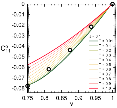
Figure 1: $C_{11}^{\alpha}=\left\langle\xi^{\alpha}\left(i\right)\xi^{\dagger}\left(i\right)\right\rangle$ , as a function of filling, $\nu$, for $J=0.1$ and temperature T ranging from 0.01 to 1. Circles are ED data extracted from Ref. [64]. $C_{11}^{\alpha}$ is proportional to the kinetic energy, $K=8tC_{11}^{\alpha}$.

3 Results

In this section, we present our numerical results. In Fig. 1, we show $C_{11}^{\alpha}=\left\langle\xi^{\alpha}\left(i\right)\xi^{\dagger}\left(i\right)\right\rangle$ as a function of electron density per site, $\nu$, for $J=0.1$ and temperature $T$ ranging from 0.01 to 1. The circles are numerical data extracted from Ref. [64] and correspond to exact diagonalization (ED) results at zero temperature for a finite cluster. There is a clear agreement with our results although we need a small finite temperature to compensate for the finite size effects. At half filling ($\nu=1$), $C_{11}^{\alpha}$ vanishes, as it is proportional to the kinetic energy by the relation $K=8tC_{11}^{\alpha}$. Since each site is occupied exactly by one electron there is no possibility for electrons to move, and kinetic energy vanishes. Our results show that the kinetic energy decreases by increasing the temperature, which means the thermally excited states of the system do not favor hole mobility, as it will be clarified in the following.

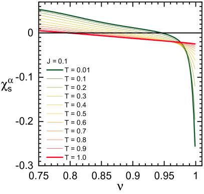
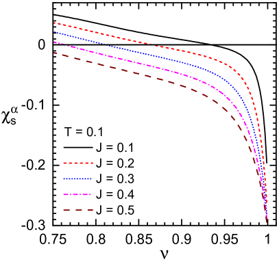
Figure 2: $\chi_{s}^{\alpha}$ as a function of $\nu$: (top) same parameters as Fig. 1; (bottom) $T=0.1$ and $J$ ranging from 0.1 to 0.5.

Although we considered a paramagnetic phase, we can still investigate the tendency of the system towards other (ordered) phases. In Fig. 2, top panel, we plot the spin-spin correlation function, $\chi_{s}^{\alpha}$, as a function of $\nu$, with same parameters as Fig. 1. For low enough temperatures, we have AF correlations near half filling. This clearly shows that our solution correctly captures the behavior in this regime, consistently with the well-established AF Nï¿œel state at half filling. The FM phase in the $t$-$J$ model has been predicted in the literature [33, 28, 34, 35, 36, 37, 29, 38, 39, 40, 41]: mobile holes can form Nagaoka polarons which results in a FM ordering [38, 40]. We witness a similar behavior here, i.e., once enough holes are present in the system, FM correlations clearly emerge and they overcome the AF ones, whose correlation lengths decrease rapidly with doping [35]. Increasing the temperature results in weakening of both AF and FM correlations: the paramagnetic phase becomes the most favorable one. Let us now come back to the decrease of the kinetic energy on increasing the temperature reported in Fig. 1. This behavior has different explanations in different doping regimes. Near half filling, the AF correlations get weaker and weaker on increasing the temperature, inhibiting the virtual hopping processes because of the Pauli exclusion principle. Accordingly, the kinetic energy decreases. On the other hand, at intermediate fillings, significant FM correlations result from the formation of Nagaoka polarons, which requires mobile holes and induce a gain in kinetic energy. By increasing the temperature, the FM correlations too become weaker and weaker and, consequently, the kinetic energy decreases also in this case.

In Fig. 2 bottom panel, we plot the spin-spin correlation function as a function of $\nu$ for $T=0.1$ and $J$ ranging from 0.1 to 0.5. For larger and larger values of $J$: $\left(i\right)$ the AF correlations increase, which shows a stronger tendency towards AF for larger exchange integrals, as expected; (ii) the emergence of FM correlations requires larger and larger values of doping in order to overcome the stronger and stronger AF correlations.

4 Summary

In summary, we performed a two-pole study of the $t$-$J$ model within COM. In our calculations, we considered the constrained electrons and their spin dressing as fundamental quasi particles. By exploiting mean-field-like approximations, we projected back the operatorial currents on the basis operators. We used similar approximations to calculate the normalization matrix within COM. These relations can be combined with the algebraic constraints obeyed by the operators to give a closed set of self-consistent equations which can be numerically solved.

Our results for the kinetic energy are in a very good agreement with those of ED for finite clusters, while our method is numerically less demanding and also more versatile. Moreover, we show that the system undergoes a smooth transition between small and intermediate doping regimes where it features AF and FM correlations, respectively. By increasing the temperature, both AF and FM correlations are weakened and, consequently, the kinetic energy decreases due to the inhibition of exchange virtual processes and polaron formation, respectively. Increasing the exchange integral strengthens the AF fluctuations, as expected, and forces the FM fluctuations to emerge at higher values of doping.

References

- [1] A. Avella, F. Mancini, Strongly Correlated Systems, Theoretical Methods, Vol. 171, Springer, 2012.
- [2] A. Avella, F. Mancini, Strongly Correlated Systems, Numerical Methods, Vol. 176, Springer, 2013.
- [3] A. Avella, F. Mancini, Strongly Correlated Systems, Experimental Techniques, Vol. 180, Springer, 2015.
- [4] J. Hubbard, Proc. R. Soc. London, Ser. A 276, 238 (1963); 277, 237 (1964); 281, 401 (1964).
- [5] P. W. Anderson, Science 235 (1987) 1196.
- [6] A. Georges, G. Kotliar, W. Krauth, M. J. Rozenberg, Rev. Mod. Phys. 68 (1996) 13.
- [7] A. Montorsi, The Hubbard Model: A Reprint Volume, World Scientific, 1992.
- [8] F. H. Essler, H. Frahm, F. Göhmann, A. Klümper, V. E. Korepin, The one-dimensional Hubbard model, Cambridge University Press, 2005.
- [9] H. Tasaki, J. Phys.: Cond. Mat. 10 (1998) 4353.
- [10] D. Baeriswyl, D. K. Campbell, J. M. Carmelo, F. Guinea, E. Louis, The Hubbard model: its physics and mathematical physics, Vol. 343, Springer Science & Business Media, 2013.
- [11] K. Chao, J. Spalek, A. M. Oles, J. Phys. C: Solid State Phys. 10 (1977) L271.
- [12] K. Chao, J. Spałek, A. M. Oles, Phys. Rev. B 18 (1978) 3453.
- [13] A. H. MacDonald, S. M. Girvin, D. Yoshioka, Phys. Rev. B 37 (1988) 9753.
- [14] J. Stein, J. Stat. Phys. 88 (1997) 487.
- [15] A. Reischl, E. Müller-Hartmann, G. S. Uhrig, Phys. Rev. B 70 (2004) 245124.
- [16] J. Spałek, Philos. Mag. 95 (2015) 661.
- [17] M. Imada, A. Fujimori, Y. Tokura, Rev. Mod. Phys. 70 (1998) 1039.
- [18] A. Avella, F. Mancini, D. Villani, Solid State Comm. 108 (1998) 723.
- [19] A. Avella, F. Mancini, D. Villani, H. Matsumoto, Euro. Phys. J. B 20 (2001) 303.
- [20] C.-W. Chen, J. Choe, E. Morosan, Rep. Prog. Phys. 79 (2016) 084505.
- [21] A. Avella, Adv. Cond. Mat. Phys. 2014 (2014) 515698.
- [22] T. Kloss, X. Montiel, V. de Carvalho, H. Freire, C. Pépin, Rep. Prog. Phys. 79 (2016) 084507.
- [23] P. A. Lee, N. Nagaosa, X.-G. Wen, Rev. Mod. Phys. 78 (2006) 17.
- [24] N. Armitage, P. Fournier, R. Greene, Rev. Mod. Phys. 82 (2010) 2421.
- [25] M. Hashimoto, I. M. Vishik, R.-H. He, T. P. Devereaux, Z.-X. Shen, Nat. Phys. 10 (2014) 483.
- [26] D. Chowdhury, S. Sachdev, in: Quantum criticality in condensed matter: Phenomena, materials and ideas in theory and experiment, World Scientific, 2016, p. 1.
- [27] S. Tajima, Rep. Prog. Phys. 79 (2016) 094001.
- [28] M. Marder, N. Papanicolaou, G. Psaltakis, Phys. Rev. B 41 (1990) 6920.
- [29] C. S. Hellberg, E. Manousakis, Phys. Rev. Lett. 78 (1997) 4609.
- [30] Y. Nagaoka, Solid State Comm. 3 (1965) 409.
- [31] Y. Nagaoka, Phys. Rev. 147 (1966) 392.
- [32] H. Tasaki, Phys. Rev. B 40 (1989) 9192.
- [33] C. Jayaprakash, H. Krishnamurthy, S. Sarker, Phys. Rev. B 40 (1989) 2610.
- [34] D. Poilblanc, Phys. Rev. B 45 (1992) 10775.
- [35] R. R. Singh, R. L. Glenister, Phys. Rev. B 46 (1992) 11871.
- [36] W. Putikka, M. Luchini, M. Ogata, Phys. Rev. Lett. 69 (1992) 2288.
- [37] H. Mori, M. Hamada, Phys. Rev. B 48 (1993) 6242.
- [38] M. Maśka, M. Mierzejewski, E. Kochetov, L. Vidmar, J. Bonča, O. Sushkov, Phys. Rev. B 85 (2012) 245113.
- [39] S. Bhattacharjee, R. Chaudhury, J. Low Temp. Phys. 193 (2018) 21.
- [40] L. Vidmar, J. Bonča, J. Supercond. Nov. Magn. 26 (2013) 2641.
- [41] R. Montenegro-Filho, M. Coutinho-Filho, Phys. Rev. B 90 (2014) 115123.
- [42] F. Mancini, A. Avella, Adv. Phys. 53 (2004) 537.
- [43] A. Avella, F. Mancini, in: Strongly Correlated Systems, Springer, 2012, p. 103.
- [44] A. Avella, Euro. Phys. J. B 87 (2014) 1.
- [45] A. Di Ciolo, A. Avella, Cond. Mat. Phys. 21 (2018) 33701.
- [46] S. Odashima, A. Avella, F. Mancini, Phys. Rev. B 72 (2005) 205121.
- [47] E. Kuz’min, S. Ovchinnikov, Teor. Mat. Fiz. 31 (1977) 379.
- [48] Y. Tserkovnikov, Teor. Mat. Fiz. 49 (1981) 219.
- [49] Y. Tserkovnikov, Teor. Mat. Fiz. 50 (1982) 261.
- [50] H. Mori, Prog. Theor. Phys. 33 (1965) 423.
- [51] D. Rowe, Rev. Mod. Phys. 40 (1968) 153.
- [52] L. Roth, Phys. Rev. 184 (1969) 451.
- [53] W. Nolting, W. Borgiel, Phys. Rev. B 39 (1989) 6962.
- [54] A. Barabanov, A. Kovalev, O. Urazaev, A. Belemuk, R. Hayn, J. Exp. Theor. Phys. 92 (2001) 677.
- [55] V. Val’kov, D. Dzebisashvili, J. Exp. Theor. Phys. 100 (2005) 608.
- [56] N. Plakida, V. Oudovenko, Phys. Rev. B 59 (1999) 11949.
- [57] N. Plakida, JETP Lett. 74 (2001) 36.
- [58] J. Exp. Theor. Phys. 97 (2003) 331.
- [59] N. Plakida, V. Oudovenko, J. Exp. Theor. Phys. 104 (2007) 230.
- [60] N. Plakida, High-temperature cuprate superconductors: Experiment, theory, and applications, Vol. 166, Springer Science & Business Media, 2010.
- [61] S. Ovchinnikov, S. Nikolaev, JETP lett. 93 (2011) 517.
- [62] A. Di Ciolo, C. Noce, A. Avella, Euro. Phys. J. Spec. Top. 228 (2019) 659.
- [63] A. Avella, F. Mancini, V. Turkowski, Phys. Rev. B 67 (2003) 115123.
- [64] E. Dagotto, A. Moreo, F. Ortolani, D. Poilblanc, J. Riera, Phys. Rev. B 45 (1992) 10741.