ROFANOVA

Robust Functional ANOVA with Application to Additive Manufacturing

Abstract

The development of data acquisition systems is facilitating the collection of data that are apt to be modelled as functional data. In some applications, the interest lies in the identification of significant differences in group functional means defined by varying experimental conditions, which is known as functional analysis of variance (FANOVA). With real data, it is common that the sample under study is contaminated by some outliers, which can strongly bias the analysis. In this paper, we propose a new robust nonparametric functional ANOVA method (RoFANOVA) that reduces the weights of outlying functional data on the results of the analysis. It is implemented through a permutation test based on a test statistic obtained via a functional extension of the classical robust $M$-estimator. By means of an extensive Monte Carlo simulation study, the proposed test is compared with some alternatives already presented in the literature, in both one-way and two-way designs. The performance of the RoFANOVA is demonstrated in the framework of a motivating real-case study in the field of additive manufacturing that deals with the analysis of spatter ejections. The RoFANOVA method is implemented in the R package rofanova, available online at https://github.com/unina-sfere/rofanova.

fabio.centofanti@unina.it

1 Introduction

The development of data acquisition methods allow the analysis of complex systems in several operating conditions as never before. Several examples may be found in the current Industry 4.0 framework, which is reshaping the variety of signals and measurements that can be gathered during manufacturing processes. Experimental data are more and more characterized by complex and novel formats, like images, videos, dense point clouds. These data may be acquired not only off line, during post-process inspections on the product, but also in line, during the production process, by exploiting a variety of sensors installed and embedded into the system. The rich information enclosed in such big data streams allows one to monitor and optimize industrial processes, as well as to improve the productivity and efficiency of production plants and enable several benefits of the ongoing digital transition. As a consequence, the focus of many applications in industrial statistics is moving from product quality characteristics to in-line process measurements, thanks to enhanced sensing and monitoring capabilities. Moreover, novel production paradigms are characterized by several controllable factors and complex process dynamics that impose the need for effective and efficient experimental approaches to determine optimal process conditions and gather deeper comprehension of underlying physical phenomena.

In this framework, a number of novel challenges shall be faced, with respect to how the quality of products is monitored, modelled and continuously improved. In many cases, statistical methods require a transformation of input data that are characterized by complex and/or high dimensional formats (e.g., multi-channel signals, images, videos, point clouds) into a format that is easier to handle and, at the same time, able to capture the information content and in order to draw reliable and robust decisions. A family of statistical methods suitable to tackle this problem is known as functional data analysis (FDA). For a comprehensive overview of FDA methods and applications we refer the reader to Ramsay (2005); Horváth and Kokoszka (2012); Kokoszka and Reimherr (2017) and, for further theoretical insights, to Hsing and Eubank (2015); Bosq (2012). FDA allows the representation of observation units in terms of functions in a 1D, 2D or higher dimensional domain with a general validity this is not limited to manufacturing applications. Such functional representation makes statistical inference methods applicable also in cases where the complexity of the input data goes far beyond traditional univariate or multivariate domains. A large variety of industrial applications where sensor signals and metrology data can be represented and analyzed as functional data have been presented so far (Noorossana and Amiri, 2011). Examples include signals with cyclic patterns, calibration curves and coordinate measurements of profiles that can be treated as 1D functions (Paynabar et al., 2013; Guo et al., 2019; Qiu et al., 2010; Colosimo and Pacella, 2010; Grasso et al., 2014). Other examples include spatial measurements and surface data that can be treated as 2D functions (Zang and Qiu, 2018; Colosimo et al., 2014). FDA resulted to be effective in modelling complex spatial or spatio-temporal patterns of image and video-image data as well, with various applications. Examples from this research line were reviewed by Megahed et al. (2011). Other examples include process monitoring and quality modelling applications where data are modelled as functional data and lead to effective anomaly detection (Wang and Tsung, 2005; Menafoglio et al., 2018; Wells et al., 2013; Capezza et al., 2021; Centofanti et al., 2021; Capezza et al., 2021; Colosimo et al., 2021).

One example of the use of FDA to translate video-image data into a functional form is presented here below and motivated the present study. It regards the analysis of process stability in a metal additive manufacturing process known as laser powder bed fusion (L-PBF) by means of high speed videos acquired during the process (Colosimo et al., 2018; Colosimo and Grasso, 2020; Grasso et al., 2021). L-PBF is an additive process suitable to produce metal parts by means of a laser beam that selectively melts thin layers of metal powder. The process is repeated layer by layer, with the material solidified in one layer being welded to the material in underneath layers, enabling the fabrication of products with complex geometries and innovative properties (Gibson et al., 2014). Fig. 1, left panel, shows an example of video frame acquired during this process. The small white particles, which are visible in the image, are spatters produced by the laser-material interaction, whereas the bigger white spot is the heat affected region where the laser is melting the material. This is just one frame of a high-speed (1000 frames per second) video, where spatters exhibit a complex time-variant dynamic pattern that is representative of the process stability. It is evident that the application of statistical inference methods to video-image data like these can be applied only if the information content is transformed, modelled or synthesised into a different format. One possible way consists of estimating synthetic quantities (like the number of spatters, their size, etc.) and translating the original video frame into a multivariate vector of descriptors (Yang et al., 2020; Andani et al., 2017; Repossini et al., 2017). This approach entails an intrinsic information loss and an arbitrary and problem dependent choice of descriptors. Another approach consists in transforming the image into a functional format. An example of this transformation is shown in Fig. 1, right panel, where a 2D function depicts spatter spread in space over the video frame. This function, which will be referred to as spatter intensity function in this study, maps the amount of spatters observed in any region of the bi-dimensional video-frame space, $(s,t)$. The term intensity here refers to the occurrence of spatters in a given location. A high spatter intensity at given spatial coordinates $(s,t)$ means that a large amount of spatters was captured in the video image stream in that specific location. Such representation allows one to capture spatial information on spatter spread in space and to make inference in a FDA fashion. The example shown in Fig. 1 can be regarded as just one of many real applications where a functional data representation is suitable to deal with complex patterns and data types. A functional representation similar to that of Fig. 1 can be suitable in all processes where spatters and hot ejections are generated, like welding or laser cutting.

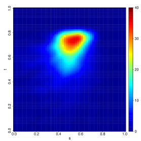
(a)	(b)

Figure 1: Example of a video frame acquired during an L-PBF process showing ejected spatters as bright spots (a) and corresponding spatter intensity function (b).

A classical statistical problem consists in the identification of significant differences in group functional means belonging to a sample with varying experimental conditions. In the literature, this problem is known as functional analysis of variance (FANOVA) that is the FDA extension of the classical (non-functional) ANOVA problem. Referring to the example in Fig. 1, the FANOVA approach may be used to study the effect of different process conditions on the spatter behaviour, which is a problem that attracted great interest in the additive manufacturing community, because the spatter behaviour can be regarded as a proxy of process stability and quality (Yang et al., 2020; Andani et al., 2017; Repossini et al., 2017; Ly et al., 2017; Bidare et al., 2018). Ramsay (2005) proposed a functional ANOVA test, based on a pointwise $F$-test statistic, that relies on the normality assumption of the error function. If the observed statistics is larger than the critical value, calculated as a percentile of the Fisher distribution, for each domain value, then the hypothesis of no differences among the groups can be safely rejected. Cuevas et al. (2004) proposed a FANOVA test based on the integrated squared difference among group functional means, for both the homoscedastic and heteroscedastic cases. The $L^{2}$-norm-based test proposed by Faraway (1997); Zhang et al. (2007) uses a statistic based on the integrated squared differences between the group mean and the global mean, whose distribution is approximately proportional to a chi-squared random variable. Shen and Faraway (2004); Zhang (2011) proposed an $F$-type test based on the fraction of the sum of the integrated squared differences between the group means and the global mean, and, the sum of the integrated squared differences between the functional observations and the group means. Under certain conditions, this statistic has a Fisher distribution. Bootstrap versions of both $L^{2}$-norm-based and $F$-type tests were proposed by Zhang (2013). Finally, Zhang and Liang (2014) introduced a globalized version of the pointwise $F$-test. Note that all the aforementioned works deal with the one-way FANOVA design.

The multi-way functional ANOVA design has been much less studied than the one-way counterpart. In particular, Brumback and Rice (1998); Guo (2002); Gu (2013) proposed tests that are able to deal with more complicated designs that rely on the use of smoothing splines (SS-ANOVA). A simple technique was proposed by Cuesta-Albertos and Febrero-Bande (2010) who transform functional data into univariate data by means of random projections. Pini et al. (2018) proposed a non‐parametric domain‐selective multi-way functional ANOVA able to identify the specific subdomains where group functional means differ. In this study, we address the functional analysis of variance in the presence of nuisance effects associated to outlying patterns in the experimental dataset. The proposed real-case study in additive manufacturing highlights the need for novel and effective methods in this framework. In the motivating case study considered by this paper, an outlying spatter ejection behaviour may be observed as a consequence of a variety of possible root causes. Fig. 2 shows an example of an outlying pattern in the spatter intensity function. For the sake of graphical clarity, functions corresponding to different realizations under the same experimental treatment are compared by looking at their cross-sections at a fixed coordinate $t$. The cross-section shown with a solid thick line in Fig. 2 represents an outlying spatter behaviour, consisting of a lower amount of spatters spread in space, possibly caused by a transient laser beam attenuation that occurred at a given point in time. Additional details about the real-case study can be found in Section 4.

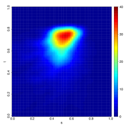
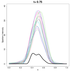
(a)	(b)	(c)

Figure 2: Example of a spatter intensity function (a), one cross-section of the spatter intensity function at t = 0.75 (b) and a superimposition of cross-sections corresponding to different experimental realizations of the spatter intensity function, where an outlying pattern is highlighted with a thick black line (c).

From a design-of-experiments perspective, outlying patterns like the one in Fig. 2 represent a nuisance, as they may inflate the variability and mask effects of potential interest. From a statistical process monitoring perspective, instead, outliers commonly drive relevant information, being potential indicators of anomalies and flaws. In this study, we refer to the former perspective, aiming at proposing an effective approach for the analysis of variance in the presence of outliers that contaminate the experimental functional data. Due to the many different dynamics involved in the process, determining whether an experimental point is an outlier and identifying its root cause can be a difficult task, but similar challenges can be faced in many different manufacturing applications, due to the complex nature of the response variables and the complex underlying physical phenomena.

All the one-way and multi-way FANOVA design cited above combine in a different quadratic fashion the functional mean to obtain the test statistic. However, as in the case of finite dimensional data, the functional mean, as well as quadratic forms, are shown to be highly sensitive to the presence of outliers. Hubert et al. (2015) set up a taxonomy of functional outliers. To deal with outliers, the diagnostic and the robust approaches are the two common alternatives. The diagnostic approach is based on standard estimates after the removal of sample units identified as outliers. Even though it is criticized as it is subject to the analyst’s personal decision, it can often be safely applied, such as in the case depicted in Fig. 2, where the marked curve can be safely deleted. However, as we will see below, it is not always easy to label an observation as outlier, especially when complex process dynamics and lack of measurable covariates make the search for root causes a difficult task. On the contrary, the robust approach produces parameter estimators as well as associated tests and confidence intervals that limit the influence of outliers on final results and decisions without the need for searching and explicitly removing them before the estimation. For a general perspective on this topic in the classical setting see Huber (2004); Hampel et al. (2011); Maronna et al. (2019).

In the very last years, several works have explored robust estimation for functional data. Fraiman and Muniz (2001) defined trimmed means for functional data based on a functional depth defined as an integral of the univariate depths for each domain value. To obtain robust estimates of the center of a functional distribution, Cuesta-Albertos and Fraiman (2006) extended the notion of impartial trimming to a functional data framework. Other location estimators based on depth functions for functional data were proposed by Cuesta-Albertos and Nieto-Reyes (2008); Cuevas and Fraiman (2009); López-Pintado and Romo (2009, 2011). The above methods are all extensions of the classical linear combination type estimators (i.e., $L$-estimator) (Maronna et al., 2019) to the functional setting. More recently, Sinova et al. (2018) extended the notion of maximum likelihood type estimators (i.e., $M$-estimators) to the functional data setting. $M$-estimators (Huber et al., 1964) are less influenced by outliers than the standard least-squares or maximum likelihood estimators, because they are based on loss functions that increase less rapidly than the usual square loss. These estimators have been applied by Kalogridis and Van Aelst (2019) to the functional linear model.

The FANOVA methods are not necessarily robust against outliers, as they rely on both the functional mean and quadratic forms, which are known to be highly sensitive to outlying observations. In the classical setting, robust ANOVA methods have been proposed by Schrader and Mc Kean (1977); Schrader and Hettmansperger (1980), who adapted Huber’s $M$-estimates to be used in a modified $F$-statistic and a likelihood ratio type test. However, to the best of our knowledge, no robust ANOVA has been introduced so far in the functional setting.

In this paper, we propose a robust functional ANOVA method (RoFANOVA) that is able to test, in a nonparametric fashion, the differences among group functional means. The RoFANOVA method is based on a functional generalization of the test statistic proposed by Schrader and Mc Kean (1977) included in a permutational framework (Good, 2013; Pesarin and Salmaso, 2010). Applications of nonparametric methods in FDA can be found in Ramsay (2005); Corain et al. (2014); Pini and Vantini (2017); Pini et al. (2018). Moreover, to obtain the test statistic, we introduce a functional extension of the normalized median absolute deviation (NMAD) estimator, referred to as functional normalized median absolute deviation (FuNMAD) estimator, as well as an equivariant version of the functional $M$-estimator proposed by Sinova et al. (2018). An extensive Monte Carlo simulation study is presented to quantify the performance of the RoFANOVA with respect to FANOVA tests already appeared in the literature before, both in one-way and two-way designs. The application of the proposed approach to the real-case study in the additive manufacturing field also highlights its effectiveness over competing methods in identifying interaction effects that are relevant to get deeper insights about the functional response variable of interest.

The paper is organized as follows. In Section 2, the robust functional analysis of variance is introduced together with the functional normalized median absolute deviation and the scale equivariant functional $M$-estimator. Section 3 presents a Monte Carlo simulation study that compares the RoFANOVA with competing methods both in one-way and two-way designs. Then, in Section 4 the RoANOVA is applied to the real-case study devoted to the study of the spatter behaviour in the L-PBF process. Conclusion is provided in Section 5. All computations and plots have been created by using R software (R Core Team, 2020). The RoFANOVA method is implemented in the R package rofanova, openly available online at https://github.com/unina-sfere/rofanova.

2 The robust functional analysis of variance

2.1 The scale equivariant functional $M$-estimator and the functional normalized median absolute deviation estimator

This section introduces the equivariant functional $M$-estimator and the functional normalized median absolute deviation estimators. Let us consider the random element $X$ with value in $L^{2}\left(\mathcal{T}\right)$, the Hilbert space of square integrable functions defined on the compact set $\mathcal{T}\subset\mathbb{R}^{p}$, with the usual norm $||f||=\left(\int_{\mathcal{T}}f^{2}\left(t\right)dt\right)^{1/2}$, for $f\in L^{2}\left(\mathcal{T}\right)$, having mean function $\mu\left(t\right)=\operatorname{E}\left[X\left(t\right)\right]$ and covariance function $\gamma\left(s,t\right)=\operatorname{Cov}\left[X\left(s\right),X\left(t\right)\right]$, for $s,t\in\mathcal{T}$. Moreover, let $\bm{X}=\left(X_{1},\dots,X_{n}\right)^{T}$ be a vector whose elements $X_{i}$ are independent realizations of $X$. Recently, Sinova et al. (2018) proposed a functional $M$-estimator of location defined as

$$\hat{\mu}_{s}=\operatorname*{argmin}_{y\in L^{2}\left(\mathcal{T}\right)}\sum_{i=1}^{n}\rho\left(||X_{i}-y||\right),$$ (1)

where $\rho:\mathbb{R}^{+}\rightarrow\mathbb{R}$ is the loss function, which is continuous, non-decreasing and satisfies $\rho\left(0\right)=0$. As shown by Sinova et al. (2018), each version of $\hat{\mu}_{s}$ is well-defined and enjoys good theoretical properties, e.g., it has maximal breakdown value and is strong consistent under suitable model assumptions. Unfortunately, these estimators are not scale equivariant. This means that, if all $X_{i}$ are equally scaled, the resulting robust estimator is not necessarily equally scaled, in analogy with the multivariate case (Maronna et al., 2019). Following Maronna et al. (2019), we propose a scale equivariant $M$-estimator of location defined as

$$\hat{\mu}=\operatorname*{argmin}_{y\in L^{2}\left(\mathcal{T}\right)}\sum_{i=1}^{n}\rho\left(\Big{\lVert}\frac{X_{i}-y}{\sigma}\Big{\lVert}\right),$$ (2)

where $\sigma\left(t\right)=\sqrt{\gamma\left(t,t\right)}$, for $t\in\mathcal{T}$. If $\sigma$ is known, the problem can be reduced to the case of a $L^{2}$ random element with $\sigma=1$. However, $\sigma$ can be rarely assumed as known, and thus it should be substituted by a robust scale estimator. In this regard, we define the FuNMAD estimator of $\sigma$ as follows

$$\operatorname{FuNMAD}\left(\bm{X}\right)=\frac{1}{c}\operatorname{Med}\left(|\bm{X}-\hat{\mu}_{s,med}|\right),$$ (3)

with $c=0.6745$ and where $\hat{\mu}_{s,med}$ denotes the functional generalization of the median obtained as the solution of the optimization problem in equation (1) with $\rho^{med}\left(\cdot\right)=|\cdot|$; $|\bm{X}-\hat{\mu}_{s,med}|=\left(|X_{1}-\hat{\mu}_{s,med}|,\dots,|X_{n}-\hat{\mu}_{s,med}|\right)^{T}$ and $\operatorname{Med}\left(\cdot\right)$ transforming a vector of functions to a function of pointwise medians. The constant $c$ makes $\operatorname{FuNMAD}$ an asymptotically pointwise consistent estimator of $\sigma$ as shown in the Supplementary Material.

Because the minimization problem in equation (1) has not a closed-form solution, Sinova et al. (2018) proposed a standard iteratively re-weighted least-squares algorithm to approximate $\hat{\mu}_{s}$. The algorithm is specifically modified to approximate $\hat{\mu}$ in equation (2) with $\sigma$ estimated through $\operatorname{FuNMAD}\left(\bm{X}\right)$, and can be summarized in the following steps.

1. Select initial weight vector $\bm{w}^{\left(0\right)}=\left(w_{1}^{\left(0\right)},\dots,w_{n}^{\left(0\right)}\right)\in\mathbb{R}^{n}$ such that $w_{i}^{\left(0\right)}\geq 0$ and $\sum_{i=1}^{n}w_{i}^{\left(0\right)}=1$.

2. Generate a sequence $\{\hat{\mu}^{\left(k\right)}\}_{k\in\mathbb{N}}$ iterating the following procedure:

   $$\hat{\mu}^{\left(k\right)}=\sum_{i=1}^{n}w_{i}^{\left(k-1\right)}X_{i},\quad\quad w_{i}^{\left(k\right)}=\frac{\psi\left(\Big{\lVert}\frac{X_{i}-\hat{\mu}^{\left(k\right)}}{\sigma}\Big{\lVert}\right)}{\sum_{i=1}^{n}\psi\left(\Big{\lVert}\frac{X_{i}-\hat{\mu}^{\left(k\right)}}{\sigma}\Big{\lVert}\right)},$$

   where $\psi$ is the first derivative of the loss function $\rho$.

3. Terminate the algorithm when, for a tolerance $\varepsilon>0$, the following condition is met

   $$\frac{|J\left(\hat{\mu}^{\left(k\right)}\right)-J\left(\hat{\mu}^{\left(k-1\right)}\right)|}{J\left(\hat{\mu}^{\left(k-1\right)}\right)}<\varepsilon,$$

   where $J\left(h\right)=\sum_{i=1}^{n}\rho\left(\Big{\lVert}\frac{X_{i}-h}{\hat{\sigma}}\Big{\lVert}\right)$.

The initial weight vector can be chosen with $w_{i}^{\left(0\right)}=\frac{\psi\left(\Big{\lVert}\frac{X_{i}-\hat{\mu}^{\left(0\right)}}{\sigma}\Big{\lVert}\right)}{\sum_{i=1}^{n}\psi\left(\Big{\lVert}\frac{X_{i}-\hat{\mu}^{\left(0\right)}}{\sigma}\Big{\lVert}\right)}$ where $\hat{\mu}^{\left(0\right)}$ is a robust initial estimate of $\mu$.

The loss function $\rho$ in equation (2) defines the properties of the resulting estimator $\hat{\mu}$. For instance, the Huber’s family of loss functions (Huber et al., 1964), which generates monotone functional $M$-estimators of location, is given by

$$\rho_{a}^{HU}\left(x\right)=\begin{cases}x^{2}/2&\text{if }0\leq x\leq a\\ a\left(x-a/2\right)&\text{if }a<x,\end{cases}$$

with tuning parameter $a>0$. It gives less importance to large errors compared to the standard least-squares loss function $\rho^{sqr}\left(x\right)=x^{2}$. Functional $M$-estimators arise from the bisquare or Tukey’s biweight family of loss functions (Beaton and Tukey, 1974) defined as

$$\rho_{a}^{BI}\left(x\right)=\begin{cases}a^{2}/6\left[1-\left(1-\left(x/a\right)^{2}\right)^{3}\right]&\text{if }0\leq x\leq a\\ a^{2}/6&\text{if }a<x,\end{cases}$$

with tuning parameter $a>0$. $M$-estimators obtained by using $\rho_{a}^{BI}$ are redescending, that is values of $x>a$ give the same contribution to the loss, regardless of their distance from $a$.

Another very used family of loss functions is the Hampel’s one (Hampel, 1974), which is defined as

$$\rho_{a,b,c}^{HA}\left(x\right)=\begin{cases}x^{2}/2&\text{if }0\leq x<a\\ a\left(x-a/2\right)&\text{if }a\leq x<b\\ \frac{a\left(x-c\right)^{2}}{2\left(b-c\right)}+a\left(b+c-a\right)/2&\text{if }b\leq x<c\\ a\left(b+c-a\right)/2&\text{if }c\leq x,\end{cases}$$

with tuning parameter $a,b,c>0$. $M$-estimators obtained by using $\rho_{a,b,c}^{HA}$ are redescending as well. Finally, the optimal family of loss functions (Maronna et al., 2019) is defined as

$$\rho_{a}^{OP}\left(x\right)=\int_{0}^{x}\left(-\frac{\Phi^{\prime}\left(|x|\right)+a}{\Phi\left(|x|\right)}\right)_{+}dx,$$

where $\Phi$ is the standard normal density, $a>0$ is a tuning parameter and $\left(t\right)_{+}$ denotes the positive part of $t$. The tuning parameters used in $\rho_{a}^{HU},\rho_{a}^{BI},\rho_{a,b,c}^{HA}$ and $\rho_{a}^{OP}$ are chosen in order to ensure given asymptotic efficiency with respect to the normal distribution (Maronna et al., 2019).

2.2 The proposed robust method for the functional analysis of variance

The aim of this section is to describe the proposed RoFANOVA for the multiway functional ANOVA design. Without loss of generality, and for ease of notation, we will focus on the two-way functional ANOVA design with interaction, but the extension to more complex designs is straightforward. To introduce the two-way functional ANOVA design with interaction, let us consider a functional response $X$, which is a random element with values in $L^{2}\left(\mathcal{T}\right)$, $\mathcal{T}\subset\mathbb{R}^{p}$, and is possibly affected by two factors, say A and B (with $I$ and $J$ levels, respectively). In this model, $X$ will be expressed as the sum of two main effects and an interaction between them, plus a random error. Our aim is to test the statistical significance of the main effects and interaction term. For $k=1,\dots,n_{ij}$, let $X_{ijk}$, denote the realizations of $X$ at level $i$ of the factor A, $i=1,\dots,I$, and level $j$ of the factor B, $j=1,\dots,J$. Then, the two-way functional ANOVA model with interaction to be tested is

$$X_{ijk}\left(t\right)=m\left(t\right)+f_{i}\left(t\right)+g_{j}\left(t\right)+h_{ij}\left(t\right)+\varepsilon_{ijk}\left(t\right)\quad t\in\mathcal{T},$$ (4)

where $m$ is the functional grand mean, which describes the overall shape of the process, $f_{i}$ and $g_{j}$ are the functional main effects and $h_{ij}$ is the interaction term. All these terms have values in $L^{2}\left(\mathcal{T}\right)$. The functional errors $\varepsilon_{ijk}$ are assumed to be independent and identically distributed random functions with zero-mean and covariance function $\gamma$. They are not required to be Gaussian. In order to make the model identifiable, we will assume that $\sum_{i=1}^{I}\sum_{j=1}^{J}n_{ij}f_{i}\left(t\right)=\sum_{j=1}^{J}\sum_{i=1}^{I}n_{ij}g_{j}\left(t\right)=\sum_{i=1}^{I}\sum_{j=1}^{J}n_{ij}h_{ij}\left(t\right)=0$. To test the significance of the coefficients in the model (4), (that is, to extend the classical ANOVA test to the functional data setting), we consider the following null and alternative hypotheses

$$H_{0,A}:f_{1}=\dots=f_{I}=\bm{0},\quad H_{1,A}:\left(H_{0,A}\right)^{C},$$ (5)

$$H_{0,B}:g_{1}=\dots=g_{J}=\bm{0},\quad H_{1,B}:\left(H_{0,B}\right)^{C},$$ (6)

$$H_{0,AB}:h_{11}=\dots=h_{IJ}=\bm{0},\quad\quad H_{1,AB}:\left(H_{0,AB}\right)^{C},$$ (7)

where $\bm{0}$ is a function almost everywhere equal to zero. The hypotheses $H_{0,A}$ against $H_{1,A}$ and $H_{0,B}$ against $H_{1,B}$ involve the effects of the main factors A and B, respectively, whereas, the hypothesis $H_{0,AB}$ against $H_{1,AB}$ involves the interaction term between them.

Each test is carried out through a nonparametric permutational approach. In this regard, we introduce a test statistic that is a functional extension of the robust F-statistic proposed by Schrader and Mc Kean (1977). The authors considered a robust version of the classical $F$-test statistic, defined as the fraction of the drop in residual sum of squares between the full model (i.e., the model when $H_{0}$ is false) and the reduced model (i.e., the model when $H_{0}$ is true), and the standard deviation of the error distribution, where all quantities are estimated by using the least-squares approach. The $F$-test statistic was modified by a specific residual sum of dispersions corresponding to a loss function as those described in Section 2.1 in place of the residual sum of squares, and a robust estimate, instead of the least-squares estimate, of the standard deviation of the error distribution.

Specifically, to test the hypotheses (5), we propose the following test statistic

$$F_{A}=\left(I-1\right)^{-1}\left[\sum_{i=1}^{I}\sum_{j=1}^{J}\sum_{k=1}^{n_{ij}}\rho\left(\Big{\lVert}\frac{X_{ijk}-\bar{X}_{r}-\bar{X}_{r,ij}+\bar{X}_{r,i\cdot}}{\hat{\sigma}_{r,e}}\Big{\lVert}\right)\right.\\ -\sum_{i=1}^{I}\sum_{j=1}^{J}\sum_{k=1}^{n_{ij}}\rho\left(\Big{\lVert}\frac{X_{ijk}-\bar{X}_{r,ij}}{\hat{\sigma}_{r,e}}\Big{\lVert}\right)\Bigg{]},$$

where $\rho$ is a given loss function, $\hat{\sigma}_{r,e}$ is a robust estimate of the functional standard deviation of the error distribution, and $\bar{X}_{r}$, $\bar{X}_{r,i\cdot}$, and $\bar{X}_{r,ij}$ are, respectively, scale equivariant functional $M$-estimators (Section 2.1) of the functional grand mean $m$, group means of $\{X_{ijk}\}_{k=1,\dots n_{ij},i=1,\dots I}$ and $\{X_{ijk}\}_{k=1,\dots n_{ij}}$. In detail, $\bar{X}_{r}$, $\bar{X}_{r,i\cdot}$, $\bar{X}_{r,ij}$ and $\hat{\sigma}_{r,e}$ are defined as

$$\bar{X}_{r} =\operatorname*{argmin}_{y\in L^{2}\left(\mathcal{T}\right)}\sum_{i=1}^{I}\sum_{j=1}^{J}\sum_{k=1}^{n_{ij}}\rho\left(\Big{\lVert}\frac{X_{ijk}-y}{\hat{\sigma}_{r}}\Big{\lVert}\right),\quad \hat{\sigma}_{r} =\operatorname{FuNMAD}\left(\{X_{ijk}\}_{\begin{aligned} \scriptscriptstyle i=&\scriptscriptstyle 1,\dots,I\\[-7.00002pt] \scriptscriptstyle j=&\scriptscriptstyle 1,\dots,J\\[-7.00002pt] \scriptscriptstyle k=&\scriptscriptstyle 1,\dots,n_{ij}\\[-7.00002pt] \end{aligned}}\right),$$

$$\bar{X}_{r,i\cdot} =\operatorname*{argmin}_{y\in L^{2}\left(\mathcal{T}\right)}\sum_{j=1}^{J}\sum_{k=1}^{n_{ij}}\rho\left(\Big{\lVert}\frac{X_{ijk}-y}{\hat{\sigma}_{r,i\cdot}}\Big{\lVert}\right),\quad \hat{\sigma}_{r,i\cdot} =\operatorname{FuNMAD}\left(\{X_{ijk}\}_{\begin{aligned} \scriptscriptstyle j=&\scriptscriptstyle 1,\dots,J\\[-7.00002pt] \scriptscriptstyle k=&\scriptscriptstyle 1,\dots,n_{ij}\\[-7.00002pt] \end{aligned}}\right),$$

$$\bar{X}_{r,ij} =\operatorname*{argmin}_{y\in L^{2}\left(\mathcal{T}\right)}\sum_{k=1}^{n_{ij}}\rho\left(\Big{\lVert}\frac{X_{ijk}-y}{\hat{\sigma}_{r,ij}}\Big{\lVert}\right),\quad \hat{\sigma}_{r,ij} =\operatorname{FuNMAD}\left(\{X_{ijk}\}_{\begin{aligned} \scriptscriptstyle k=&\scriptscriptstyle 1,\dots,n_{ij}\\[-7.00002pt] \end{aligned}}\right),$$

$$\hat{\sigma}_{r,e}=\frac{1}{0.6745}\operatorname{Med}\left(|\{X_{ijk}-\bar{X}_{r,ij}\}_{\begin{aligned} \scriptscriptstyle i=&\scriptscriptstyle 1,\dots,I\\[-7.00002pt] \scriptscriptstyle j=&\scriptscriptstyle 1,\dots,J\\[-7.00002pt] \scriptscriptstyle k=&\scriptscriptstyle 1,\dots,n_{ij}\\[-7.00002pt] \end{aligned}}|\right).$$

The test statistic $F_{A}$ represents the mean difference between the standardized residual sum of dispersions under the reduced model and the full model, and is analogous to that used by Schrader and Mc Kean (1977) in the classical setting. Intuitively, it is a measure of the discrepancy between residuals of the model under $H_{0,A}$ and under $H_{1,A}$, obtained through robust statistics. Analogously, to test the hypotheses (6) and (7), we define

$$F_{B}=\left(J-1\right)^{-1}\left[\sum_{i=1}^{I}\sum_{j=1}^{J}\sum_{k=1}^{n_{ij}}\rho\left(\Big{\lVert}\frac{X_{ijk}-\bar{X}_{r}-\bar{X}_{r,ij}+\bar{X}_{r,\cdot j}}{\hat{\sigma}_{r,e}}\Big{\lVert}\right)\right.\\ -\sum_{i=1}^{I}\sum_{j=1}^{J}\sum_{k=1}^{n_{ij}}\rho\left(\Big{\lVert}\frac{X_{ijk}-\bar{X}_{r,ij}}{\hat{\sigma}_{r,e}}\Big{\lVert}\right)\Bigg{]},$$

$$F_{AB}=\left(\left(I-1\right)\left(J-1\right)\right)^{-1}\left[\sum_{i=1}^{I}\sum_{j=1}^{J}\sum_{k=1}^{n_{ij}}\rho\left(\Big{\lVert}\frac{X_{ijk}-\bar{X}_{r,i\cdot}-\bar{X}_{r,\cdot j}+\bar{X}_{r}}{\hat{\sigma}_{r,e}}\Big{\lVert}\right)\right.\\ -\sum_{i=1}^{I}\sum_{j=1}^{J}\sum_{k=1}^{n_{ij}}\rho\left(\Big{\lVert}\frac{X_{ijk}-\bar{X}_{r,ij}}{\hat{\sigma}_{r,e}}\Big{\lVert}\right)\Bigg{]},$$

where

$$\bar{X}_{r,\cdot j} =\operatorname*{argmin}_{y\in L^{2}\left(\mathcal{T}\right)}\sum_{i=1}^{I}\sum_{k=1}^{n_{ij}}\rho\left(\Big{\lVert}\frac{X_{ijk}-y}{\hat{\sigma}_{r,\cdot j}}\Big{\lVert}\right),\quad \hat{\sigma}_{r,\cdot j} =\operatorname{FuNMAD}\left(\{X_{ijk}\}_{\begin{aligned} \scriptscriptstyle i=&\scriptscriptstyle 1,\dots,I\\[-6.3pt] \scriptscriptstyle k=&\scriptscriptstyle 1,\dots,n_{ij}\\[-6.3pt] \end{aligned}}\right).$$

Different versions of the proposed test statistics may emerge by the choice of the loss function $\rho$ as defined in Section 2.1, and by the use of $\hat{\sigma}_{r,ij}=\hat{\sigma}_{r,e}$ to estimate $\bar{X}_{r,ij}$.

Another element to choose in a permutation test is the approximation method for the distribution of the considered statistic under the null hypothesis. In our case, we selected the Manly’s scheme (Gonzalez and Manly, 1998; Manly, 2006) that consists of simply permuting the raw data without restrictions. Although other schemes could be used, the Manly’s one has demonstrated good performance and simplicity, especially when the sample size, at given factor levels, is small. See Gonzalez and Manly (1998) and Anderson (2001) for further details.

Lt $F$ generically denotes the statistic (resp., $F_{A}$ or $F_{B}$ or $F_{AB}$) to test, at level $\alpha$, $H_{0}$ against $H_{1}$ (resp., $H_{0,A}$ against $H_{1,A}$; or $H_{0,B}$ against $H_{1,B}$; or $H_{0,AB}$ against $H_{1,AB}$). Then, the proposed permutation test can be outlined by the following steps.

1. Compute the observed value of the test statistic $F_{obs}$, by considering the original sample $\{X_{ijk}\}_{k=1,\dots n_{ij},i=1,\dots I,j=1,\dots J}$.

2. Randomly permute the data, among the Factor A and Factor B combinations, $B$ times, and for each permuted sample compute the value $F^{*}_{1},\dots,F^{*}_{B}$ of the statistic $F$.

3. Compute the approximated p-value as

   $$p=\frac{1}{B}\sum_{i=1}^{B}I\left(F^{*}\geq F_{obs}\right),$$

   where $I\left(E\right)$ takes values 1 or 0 depending on whether E is true or false.

4. Accept $H_{0}$ if $p>\alpha$, otherwise reject $H_{0}$.

This is an approximate (asymptotically exact) level-$\alpha$ test for $H_{0}$ against $H_{1}$ (Anderson, 2001). The larger the number of permutations $B$, the lower the approximation error. We suggest to select the number of permutations $B$ equal to or larger than 1000 (Good, 2013).

3 Simulation study

In this section, by means of an extensive Monte Carlo simulation study, the performance of the proposed method is assessed in terms of empirical size and power of the test. In particular, the following two scenarios are investigated:

1. A one-way FANOVA model (i.e., model (4) with $m=0$, $g_{1}=\dots=g_{J}=0$ and $h_{11}=\dots=h_{IJ}=0$) is considered (Section 3.1).

2. A two-way FANOVA model (i.e., model (4)) is considered (Section 3.2).

In each scenario, the FANOVA model is contaminated by different type of outlying curves. To do so, we use the same contamination models as in previous works on robust FDA (Fraiman and Muniz, 2001; López-Pintado and Romo, 2009; Sinova et al., 2018). All the details about the data generation process are provided in the Supplementary Materials.

3.1 One-way functional analysis of variance

The proposed simulation study framework for one-way FANOVA has been inspired by Cuevas et al. (2004); Górecki and Smaga (2015). Three different model M1, M2 and M3, with 3 level main effect $f_{i}$, $i=1,2,3$, are considered, and without loss of generality, we assume the curve domain $\mathcal{T}=\left[0,1\right]$. Model M1 corresponds to $H_{0}$: $f_{1}=f_{2}=f_{3}$ true, whereas, M2 and M3 provide examples, with $H_{0}$ false, of monotone functions with different increasing patterns. In particular, M2 simulates $f_{i}$ differences that are smaller than M3, where $f_{i}$ are quite separated. In model M1, we use as performance measure the empirical size, whereas in M2 and M3 we use the empirical power. Moreover, to simulate different types of outlying curves, seven contamination models denoted by C0-6 are considered. The model C0 is representative of no contamination. C1-4 represents magnitude contaminations, i.e., curves are generated far from the center, with, in particular, C1-2 (resp., C3-4) representing symmetric and partial trajectory contamination models, that are independent (resp., dependent) from the level of the main effect. Models C5-6 are shape contamination models (López-Pintado and Romo, 2009; Sinova et al., 2018).

In all the cases considered, the response curves are independent realizations of a Gaussian process with covariance function $\gamma\left(s,t\right)=\sigma^{2}e^{\left(-|s-t|10^{-5}\right)}$ and are observed through $25$ evenly spread discrete points with $\sigma$ equal to $\sigma_{1}=1/25$, $\sigma_{2}=1.8/25$, $\sigma_{3}=2.6/25$, $\sigma_{4}=3.4/25$, $\sigma_{5}=4.2/25$, $\sigma_{6}=5/25$ (Cuevas et al., 2004). We expect that the higher $\sigma$, the worse the performance in terms of both empirical size and power. Five versions of the RoFANOVA method are considered, which are defined by different choices of the loss function, viz., the RoFANOVA with median loss $\rho^{med}$, referred to as RoFANOVA-MED, Huber loss $\rho_{a}^{HU}$, referred to as RoFANOVA-HUB, bisquare loss $\rho_{a}^{BI}$, referred to as RoFANOVA-BIS, Hampel loss $\rho_{a,b,c}^{HA}$, referred to as RoFANOVA-HAM, and, optimal loss $\rho_{a}^{OP}$, referred to as RoFANOVA-OPT. The tuning constants are chosen to achieve $95\%$ asymptotic efficiency, the number of permutations $B$ are set equal to $1000$ and the functional $0.8\%$ deepest curve following the FM criteria (Febrero-Bande and Oviedo de la Fuente, 2012) is chosen as starting value to compute the robust equivariant functional $M$-estimators (Section 2.1). The proposed tests are compared with some non-robust methods already appeared in the literature before. In particular, we consider the method proposed by Górecki and Smaga (2015), referred to as FP, which is a permutation test that relies on a basis function representation of the response function; the method proposed by Zhang and Liang (2014), referred to as GPF, based on a globalized version of the pointwise $F$-test; the method proposed by Zhang et al. (2007), referred to as L²B, a $L^{2}$-norm-based test with the bias-reduced method to estimate the unknown parameters; and the method proposed by Zhang (2011), referred to as FB, which is an $F$-type test based on the bias-reduced estimation method. All these methods are implemented with the default settings of the R package fdANOVA (Gorecki and Smaga, 2018). In addition, the method proposed by Cuesta-Albertos and Febrero-Bande (2010), based on randomly chosen one-dimensional projections, with both the Bonferroni (referred to as TRPbon) and the false discovery rate (referred to as TRPfdr) corrections, is considered. The TRPbon and TRPfdr are run with 30 random projections through the R package fda.usc (Febrero-Bande and Oviedo de la Fuente, 2012).

For each triplet (M$l$,C$m$,$\sigma_{n}$), $l=1,\dots,3$, $m=0,\dots,6$, $n=1,\dots,6$, the five proposed and the seven competing methods are applied $N=500$ times to the generated functional sample to test $H_{0}$: $f_{1}=f_{2}=f_{3}$ against $H_{1}$: $(H_{0})^{C}$ at level $\alpha=0.05$. Then, for each case, the empirical sizes (for model M1) and powers (for models M2 and M3) of the tests were computed as the proportion of rejections out of the $N$ replications whose standard deviation is equal at most to 0.0224, which corresponds to the case of probability of rejection equal to 0.5.

Fig. 3 displays the results for model M1, that is the empirical size of the eleven tests as a function of $\sigma_{n}$, $n=1,\dots,6$, for contamination models C0-6.

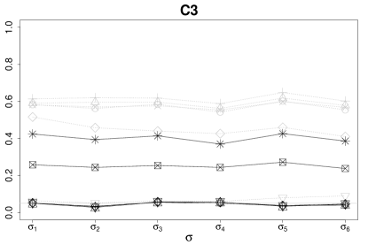
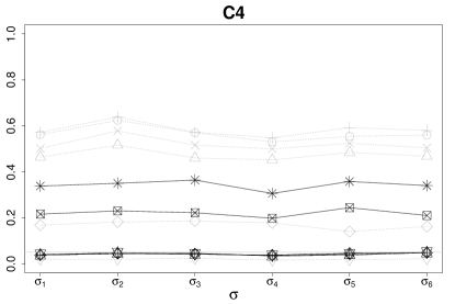
Figure 3: Empirical size of all tests for $H_{0}$ against $H_{1}$ (at level $\alpha=0.05$) as a function of $\sigma_{n}$, $n=1,\dots,6$, for contamination models C0-6 in model M1 of Scenario 1. The proposed and competing tests are displayed as black and grey lines, respectively.

In this case, the tests provide satisfactory results in controlling the level $\alpha$, i.e., the empirical size is approximately less than or equal to $0.05$, in case of no contamination (C0), symmetric magnitude contamination (C1-2) and shape contamination, both symmetric (C5) and asymmetric (C6). On the contrary, for asymmetric magnitude contamination (C3-4), only the RoFANOVA tests based on redescending loss functions, i.e., RoFANOVA-BIS, RoFANOVA-HAM and RoFANOVA-OPT, are able to control the level $\alpha$ by ensuring an empirical size approximately less or equal than $0.05$. This was somehow expected, as it is known that rededescending estimators give no weight to observations that are far from the center (Maronna et al., 2019). The estimators used in RoFANOVA-MED and RoFANOVA-HUB tests do not have this property and, thus, they suffer from the presence of contaminations depending on the level of the main factor. Note that, among the competitors, the TRPbon approximately controls the level for contamination model C4, while it is slightly affected by outliers in model C5. This comes from the Bonferroni correction property of being conservative for high-dimensional multiple comparisons (Lehmann and Romano, 2006).

Fig. 4 shows the results for model M2 in terms of empirical power. These tend to get worse as $\sigma_{n}$ increases. In case of no contamination (C0), the FP test achieves the largest empirical power, even though all RoFANOVA tests have comparable results. For contamination model C1-6, it is extremely clear the proposed RoFANOVA tests outperform all competitors. In particular, among RoFANOVA tests, those based on redescending functional $M$-estimators (viz., RoFANOVA-BIS, RoFANOVA-HAM and RoFANOVA-OPT) are the best ones. Note that, for contaminations C3-4, only the RoFANOVA-BIS, RoFANOVA-HAM and RoFANOVA-OPT tests and the TRPbon test (only for C4) should be considered, because all the other methods are not able to successfully control the level $\alpha$ (see Fig. 3).

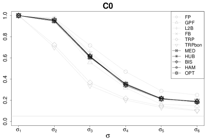
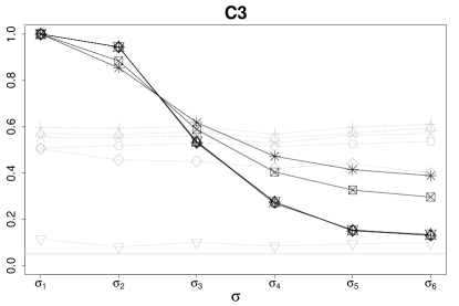
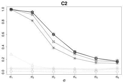
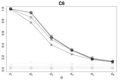
Figure 4: Empirical power of all tests for $H_{0}$ against $H_{1}$ (at level $\alpha=0.05$) as a function of $\sigma_{n}$, $n=1,\dots,6$, for contamination models C0-6 in model M2 of Scenario 1. The proposed and competing tests are displayed as black and grey lines, respectively.

Fig. 5 shows the empirical power for model M2 generally become smaller when $\sigma_{n}$ increases. The results are similar to those for model M2, even though the empirical power tends to be larger, due to the more apparent separation of the main effects. Again, the proposed RoFANOVA tests outperform the competitors in case of contamination (C1-6), and have satisfactory power in case of no contamination (C0). The best results are achieved by the RoFANOVA-BIS, RoFANOVA-HAM and RoFANOVA-OPT tests.

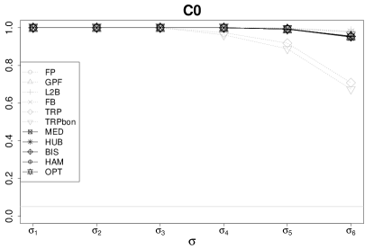
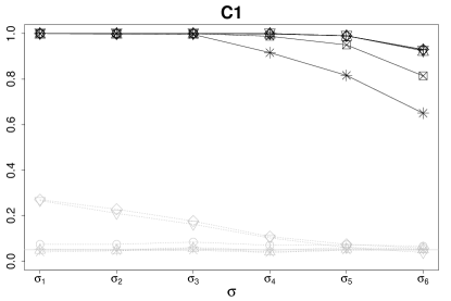
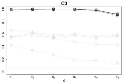
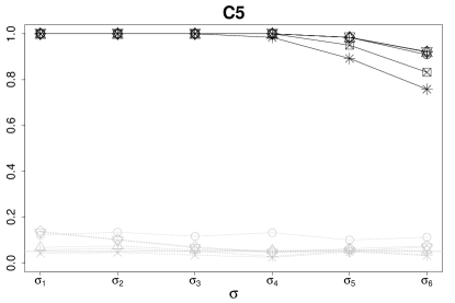
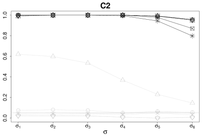
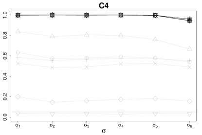
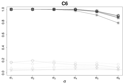
Figure 5: Empirical power of all tests for $H_{0}$ against $H_{1}$ (at level $\alpha=0.05$) as a function of $\sigma_{n}$, $n=1,\dots,6$, for contamination models C0-6 in model M3 of Scenario 1. The proposed and competing tests are displayed as black and grey lines, respectively.

3.2 Two-way functional analysis of variance

In this section, we consider the two-way FANOVA model introduced in equation (4). The simulation design is inspired by that of Cuesta-Albertos and Febrero-Bande (2010).

As for Scenario 1, we assume $\mathcal{T}=\left[0,1\right]$ and the functional response depending on a grand mean $m$, 2 level main effects $f_{i}$ and $g_{i}$, and on an interaction term $h_{ij}$ through two parameters $a$ and $b$ with values in $\{0,0.05,0.10,0.25,0.50\}$. Here, the larger the values of $a$ and $b$ the more $f_{i}$ and $g_{i}$ deviate, respectively, from the grand mean $m$. Thus, the empirical power should be an increasing function of $a$ and $b$. The empirical size is studied for $a=0$ or $b=0$.

As in Scenario 1, seven contamination models C0-6 are considered, and the response curves are assumed as independent realizations of a Gaussian process with covariance function $\gamma\left(s,t\right)=\sigma^{2}e^{\left(-|s-t|10^{-5}\right)}$. Data are observed through $25$ evenly spread discrete points with $\sigma=0.3$. Also in this scenario, we consider the five versions of the proposed method, viz., RoFANOVA-MED, RoFANOVA-HUB, RoFANOVA-BIS, RoFANOVA-HAM, and RoFANOVA-OPT, with tuning parameters chosen as in Scenario 1. As competitors we consider: (i) the permutation version of the method proposed by Zhang (2011), referred to as FNDP, which is permutation test based on a $F$-type statistic; and (ii) the global version of the method proposed by Pini and Vantini (2017), which is the two-way extension of the method of Zhang and Liang (2014), referred to as TGPF. Both for the FNDP and TGPF methods, the distribution of the test statistic is approximated by using the Manly’s scheme (Manly, 2006) with 1000 random permutations. Moreover, also the TRPbon and TRPfdr method (Section 3.1) are considered with 30 random projections.

For each triplet (C$m$,$a$,$b$), with $m=0,\dots,6$, and $a,b\in\{0,0.05,0.10,0.25,0.50\}$, the five proposes and the four competing methods are applied $N=500$ times to the generated functional sample to test, at level $\alpha=0.05$, $H_{0,A}$, $H_{0,B}$ and $H_{0,AB}$ against $H_{1,A}$, $H_{1,B}$ and $H_{1,AB}$, respectively. Then, for each triplet and test, the empirical size and empirical power of the test were computed as the fraction of rejections out of $N$ replications (also in this case, with maximum standard deviation equal to 0.0224). The former is considered when $a=b=0$, for $H_{0,A}$, $H_{0,B}$ against $H_{1,A}$, $H_{1,B}$, and when $a<0.25$ for $H_{0,AB}$ against $H_{1,AB}$; whereas the latter is considered when $a\neq 0$ or $b\neq 0$, for $H_{0,A}$, $H_{0,B}$ against $H_{1,A}$, $H_{1,B}$, and $a\geq 0.25$ for $H_{0,AB}$ against $H_{1,AB}$.

For the sake of conciseness, we summarize the results for cases that are statistically equivalent. For instance, when analyzing the null hypothesis $H_{0,A}$ (resp., $H_{0,B}$), for each value of $a$ (resp., $b$), the five values corresponding to $b=\{0,0.05,0.10,0.25,0.50\}$ (resp., $a=\{0,0.05,0.10,0.25,0.50\}$) are summarized through their median. Similarly, when analyzing $H_{0,AB}$, the values corresponding to $a<0.25$ are substituted by their median for each value of $b$.

Fig. 6 shows the empirical size ($a=0$) and power ($a\neq 0$) of all tests for $H_{0,A}$ against $H_{1,A}$ as a function of $a$. When $a$ increases, the performance of all the methods in rejecting $H_{0,A}$ enhances. In terms of empirical size (i.e., when $a=0$), the results are quite satisfactory for all the methods in case of no contamination (C0), symmetric magnitude contamination (C1-2) and both symmetric (C5) and asymmetric (C6) shape contamination. However, in case of asymmetric magnitude contamination (C3-4), only the RoFANOVA-BIS, RoFANOVA-HAM and RoFANOVA-OPT tests are able to control the level $\alpha$, being approximately less than or equal to 0.05. This behavior is analogous to that achieved in Scenario 1 of Section 3.1. In terms of empirical power ($a\neq 0$), the proposed RoFANOVA test has comparable performance when there are no outliers (C0); whereas it is far better than the competitors for the contamination models C1-6. Note that, for asymmetric magnitude contamination (C3-4), only the RoFANOVA-BIS, RoFANOVA-HAM and RoFANOVA-OPT tests should be considered, being the only ones able to control the level $\alpha$.

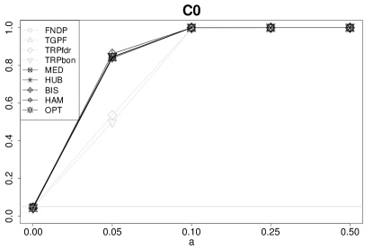
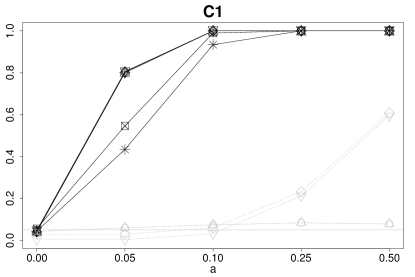
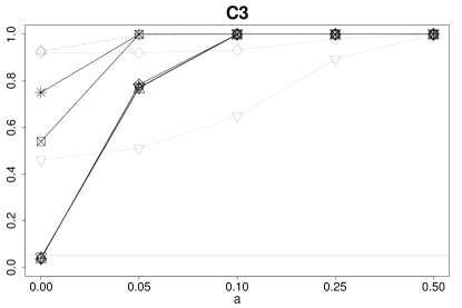
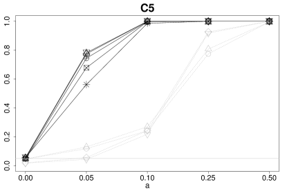
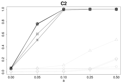
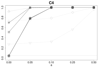
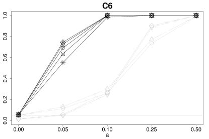
Figure 6: Empirical size ($a=0$) and power ($a\neq 0$) of all tests for $H_{0,A}$ against $H_{1,A}$ (at level $\alpha=0.05$) as a function of $a$, for different contamination models (C0-6) in Scenario 2. The proposed and competing tests are displayed as black and grey lines, respectively.

In Fig. 7, the empirical size ($b=0$) and the empirical power ($b\neq 0$) of all tests for $H_{0,B}$ against $H_{1,B}$ (at level $\alpha=0.05$) are displayed as a function of $b$. Also in this case, the proposed tests outperform the competitors, in terms of power, for contamination models C1-6. They simultaneously have, in fact, comparable performance in absence of contamination (C0). Moreover, differently from Scenario 1, all the tests are able to approximately control the level $\alpha$, even for the contamination models C3-4. This is expected in this case, because the asymmetry in the contamination affects the main effect $f_{i}$, only, and not $g_{i}$. Among the proposed tests, the RoFANOVA-BIS, RoFANOVA-HAM and RoFANOVA-OPT tend to perform better than the ones based on monotonic functional $M$-estimator, viz., the RoFANOVA-MED and RoFANOVA-HUB tests.

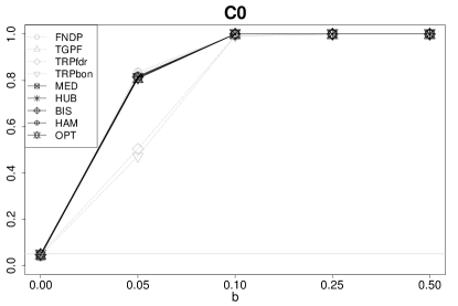
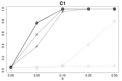
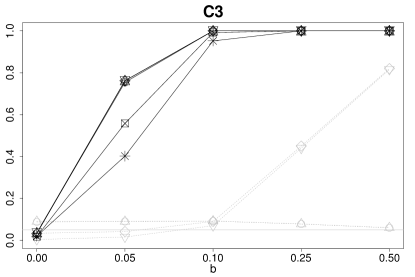
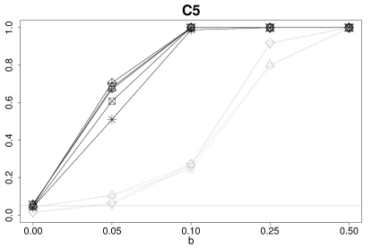
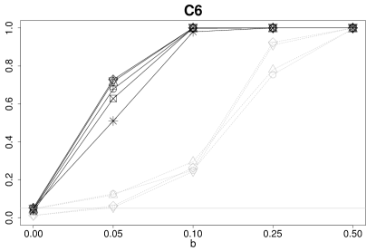
Figure 7: Empirical size ($b=0$) and power ($b\neq 0$) of all tests for $H_{0,B}$ against $H_{1,B}$ (at level $\alpha=0.05$) as a function of $b$, for different contamination models (C0-6) in Scenario 2. The proposed and competing tests are displayed as black and grey lines, respectively.

To test $H_{0,AB}$ against $H_{1,AB}$, results are presented in the Supplementary Material where it is shown that the empirical power of the proposed tests is much larger than that of the competitors, for all the contamination model C1-6. Moreover, and that among the RoFANOVA tests, the RoFANOVA-BIS, RoFANOVA-HAM and RoFANOVA-OPT achieve the best performance.

4 Real-case study: analysis of variance of applied to the analysis of spatter behaviour in laser powder bed fusion

To demonstrate the potential of the proposed approach, this Section presents the real-case study in additive manufacturing. In L-PBF, spatters are process by-products that can be ejected either by the melt pool, i.e., the region when the thin layer of powder is locally melted by the laser, in the form of hot and liquid droplets or by the powder bed regions surrounding the melt pool (Young et al., 2020; Ly et al., 2017; Bidare et al., 2018). In the latter case, spatters consist of powder particles entrained by convective motions above and around the melt pool. For more details about the spatter generation mechanism, the reader is referred to Young et al. (2020); Ly et al. (2017); Bidare et al. (2018), and the literature cited therein. The analysis of spatters in the L-PBF process has gathered an increasing interest in the last years because they can drive relevant information about the process state and the final quality of the manufactured part. Studying the effect of controllable process factors and other operating conditions on the spatter behaviour allows getting a deeper comprehension of underlying physical phenomena. Such knowledge may be used to tune the process condition and enhance the quality and mechanical performances of the products, or to design in-line and real-time process monitoring methodologies (Colosimo and Grasso, 2020).

Hot spatters ejected as a consequence of the laser-material interaction can be observed by means of high-speed cameras installed into the L-PBF machine or placed outside its viewports. The mainstream literature devoted to spatter analysis and monitoring in L-PBF relies on video image processing methods to compute synthetic indices that capture salient aspects of the spatter behaviour, e.g., the number of ejected spatters in each video frame, their size, speed, etc. (Grasso et al., 2017; Everton et al., 2016). In the real-case study presented in this section, instead of treating synthetic descriptors of the spatter ejections as univariate or multivariate variables, the spatter behaviour is translated into a functional format by means of the so-called spatter intensity function introduced in Section 1. Such function captures the spatial spread of ejected spatters and can be estimated for each manufactured layer and for each test treatment. Section 4.1 presents the main experimental settings, whereas the results of the analysis and the comparison against benchmark methods are reported in Section 4.2.

4.1 Experimental setting and data preprocessing

The case study involves the production of specimens of size 5 x 5 x 12 mm via L-PBF of 18Ni(300) maraging steel powder, a steel alloy commonly used for tooling applications, with average particle size between 25 and $35\mu$m. An industrial L-PBF system, namely a Renishaw AM250, was used, with a high-speed camera in the visible range placed outside the front viewport of the machine as shown in Fig. 8, left panel. Videos were recorded during the production of six layers with a sampling rate of 1000 fps (frames per second) and a spatial resolution of about $200\mu$m/pixel. Specimens are placed as shown in Fig. 8, right panel, and produced by varying the energy density provided by the laser to the material. Process parameters corresponding to the energy density levels are reported in the Supplementary Material.

The laser was displaced by a scanner along a predefined path consisting of parallel scan lines, whose orientation changed layer by layer, with a default rotation of about $67^{\circ}$ every layer. Details about locations and orientations of the six analysed layers are provided in the Supplementary Material. Along each scan line, the laser melts the material with a pulsed mode, i.e., by exposing points equispaced apart of a quantity $d$ along each scan line with a point exposure duration $t$. The energy density was varied by varying $t$ and $d$. Within the build chamber, where the L-PBF process takes place, a laminar flow of inert gas, called shielding gas, is used to prevent ejected spatters from falling on the build area, with consequent potential contamination effects, and vaporized material from depositing on the laser window leading to possible attenuation of the laser beam (Anwar and Pham, 2018).

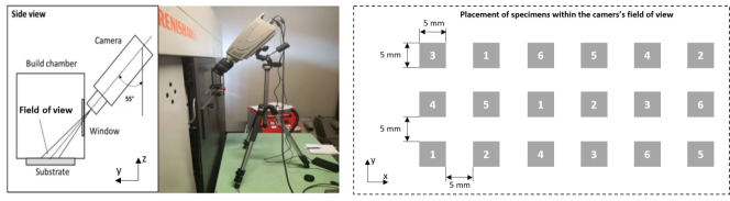
Figure 8: Setup of the high-speed camera in front of the Renishaw AM250 machine’s viewport (left panel) and placement of manufactured specimens in the build area, within the camera’s field of view (right panel): numbers shown in the specimens correspond to the energy density level, from 1 to 6, applied during the process.

The functional response variable is the spatter intensity and was estimated by applying the video image pre-processing method presented in Repossini et al. (2017). Thanks to this approach, the centroid of each spatter in the video frame was computed and used to determine the spatial coordinates $(s,t)$ of each detected spatter. All details about the video image pre-processing steps can be found in Repossini et al. (2017). In order to spatially map the amount of spatters ejected during the production of each specimen in each layer, three additional pre-processing operations were performed. First, the location of spatters was referred to a spatial domain centered in the center of the scanned area of each specimen, to allow comparing the functional response variables for specimens produced in different locations. Second, the spatial domain was discretized into 60 by 80 adjacent squared cells, in order to count the number of spatters ejected in each layer within each cell. Based on these pre-processing steps, the spatial spread of the spatters, in each layer and for each specimen, could be summarized into the function $Y_{i,j,k}\left(s,t\right)$ defined on the bi-dimensional domain $\mathcal{T}=\left[0,1\right]\times\left[0,1\right]$, where indices $i=1\dots,6$, $j=1,\dots 6$ and $k=1,\dots,n_{ij}$ indicate the energy density level, the layer, and the number of replicates (specimens) for each treatment, respectively. The spatter intensity function $Y_{i,j,k}\left(s,t\right)$ is a smoothed version of the actual amount of spatters counted in every location of the spatial domain. The number of replicates $n_{ij}$ is fixed and equal to 3, as three specimens were produced for each energy density level, except for $i=6$ and $j=1$ where $n_{ij}=2$, due to a delamination occurred in initial layers prevented from producing one of the three specimens with the lowest energy density level. The $Y_{i,j,k}$ are obtained by means of a smoothing phase based on tensor product bases of cubic splines, with second derivative penalty as marginal smooths. The marginal basis dimensions, set equal to 30, and the smoothing parameters were chosen by using restricted maximum likelihood (REML) (Wood, 2017). The smoothing phase was performed by using the R package mgcv (Wood, 2017). Then, in order to reduce phase variability, a registration phase was performed (Ramsay, 2005). It consists in the shifting of each $Y_{i,j,k}$ along the $s$ and $t$ axes to minimize the $L^{2}$ distance with respect to the reference curve, which was chosen such that the mean of pairwise distances among the aligned curves is minimum. The functional observations $Y_{i,j,k}$, $i=1\dots,6$, $j=1,\dots 6$ and $k=1,\dots,n_{ij}$, for $t=0.75$ and $s=0.5$ are represented in Fig. 9 at different energy density levels and in different layers. The graphical representation of cross-sections of the spatter intensity function in Fig. 9 was adopted to aid the superimposition and direct comparison of functional patterns corresponding to different experimental treatments.

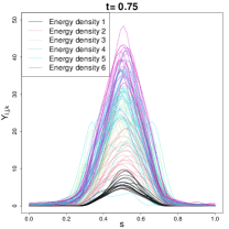
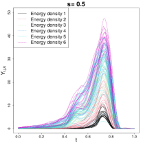
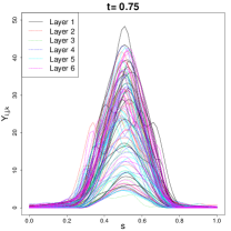
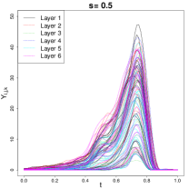
(a)	(b)	(c)	(d)

Figure 9: The functional observations $Y_{i,j,k}$ for $t=0.75$, (a) and (c), and $s=0.5$, (b) and (d), in the real-case study, for different energy density levels ((a) and (b)) and different scan strategies ((c) and (d)).

4.2 Results

The spatter intensity functions $Y_{i,j,k}$ ($i=1\dots,6$, $j=1,\dots 6$ and $k=1,\dots,n_{ij}$) are modeled according to equation (4), where $f_{i}$ is the energy density functional effect, $g_{i}$ is the layer functional effect, $h_{ij}$ is the interaction term between the energy density and the layer. The equivariant functional M-estimators (Section 2.1) are shown in the Supplementary Material.

The aim of the analysis is therefore to test the energy density effect $H_{0,Flu}=H_{0,A}$ (5), the layer effect $H_{0,Lay}=H_{0,B}$ (6) (mainly related to the layer by layer variation of the laser scan direction) and their interaction effect $H_{0,FluLay}=H_{0,AB}$ against the alternatives $H_{1,Flu}=H_{1,A}$ (5), $H_{1,Lay}=H_{1,B}$ (6) and $H_{1,FluLay}=H_{1,AB}$. In particular, Fig. 10 shows (a) the residuals of the fitted model for $t=0.75$ (the approximate $t$ value of the spatter intensity peak), obtained by using the RoFANOVA-BIS test as implemented in Section 3, and (b) the boxplot of their $L^{1}$ norms, defined as $||f||_{1}=\int_{\mathcal{T}}|f\left(t\right)|dt$, for $f\in L^{2}\left(\mathcal{T}\right)$. Because $\mathcal{T}=\left[0,1\right]\times\left[0,1\right]$, the $L^{1}$ norm can be interpreted as the average value of the function over its domain. It is clear from Fig. 10 that some outliers are present in this real-case study. However, except from a few residuals that plot far from the bulk of the data, there are some points that could not be easily labeled as outliers. As mentioned in the introduction, the L-PBF process is characterized by complex dynamics with many transient and local phenomena that not only affect the natural variability of the measured quantities, but could lead also to outlying patterns. Determining whether an experimental point is an outlier or not, and identifying its root causes can be a difficult task, which makes the diagnostic approach hardly applicable in the absence of additional data and information.

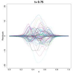
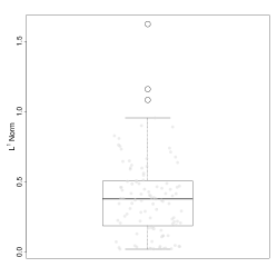
(a)	(b)

Figure 10: (a) Residuals of the fitted model for $t=0.75$, obtained by using the RoFANOVA-BIS test as implemented in Section 3, and (b) boxplot of their $L^{1}$ norms.

Therefore, we applied the RoFANOVA test described in Section 3, viz, RoFANOVA-MED, RoFANOVA-HUB, RoFANOVA-BIS, RoFANOVA-HAM, and RoFANOVA-OPT, specifically adapted for bi-dimensional functional data. As in the Monte Carlo simulation study (Section 3), the tuning constants are chosen such that the $95\%$ asymptotic efficiency is achieved, the number of permutations $B$ are set equal to $1000$. The functional sample mean is used as starting value to compute the robust equivariant functional $M$-estimators (Section 2.1). The results are shown in Table 1. All the tests agree in considering significant the interaction between the energy density and the layer.

Table 1: p-values of the RoFANOVA tests for $H_{0,Flu}$, $H_{0,Lay}$ and $H_{0,FluLay}$ against $H_{1,Flu}$, $H_{1,Lay}$ and $H_{1,FluLay}$.

	RoFANOVA-MED	RoFANOVA-HUB	RoFANOVA-BIS	RoFANOVA-HAM	RoFANOVA-OPT
$H_{0,FluLay}$	0.00	0.01	0.00	0.00	0.00
$H_{0,Flu}$	0.00	0.00	0.00	0.00	0.00
$H_{0,Lay}$	0.00	0.00	0.00	0.00	0.00

When an the interaction effect is present, it is well-known that an interpretation of the main effects becomes less straightforward than if the interaction is not significant (Miller Jr, 1997), because the layer effect upon the spatter intensity will differ depending on the energy density level. In this case, the best way to interpret the results is through the interaction plot (Montgomery, 2017), which graphically represents the response means at different factor levels. Fig. 11 shows an interaction plot adapted to deal with bi-dimensional data. In particular, the $L^{1}$ norms of the group means, corresponding to the RoFANOVA-BIS test, are plotted as a function of the energy density level and the layer. In this case, if an interaction is present, the trace of the average response across the levels of one factor, which is plotted separately for each level of the other factor, will not be parallel (Montgomery, 2017). Fig. 11 shows that, as the energy density increases, the spatter intensity tends to increase as well. This is in agreement with the fact that a higher energy density generates a larger and hotter melt pool with more intense convective and recoil motions, which translates into a more intense spatter ejection (Yang et al., 2020; Repossini et al., 2017; Bidare et al., 2018). More interestingly, Fig. 11 shows different patterns corresponding to different layers. Indeed, in layers 1, 2, and 6, the spatter intensity is increasing with respect to the energy density. These three levels were characterized by very similar laser scan directions, with a low angle relative to the shielding gas flow (between $10^{\circ}$ and $40^{\circ}$). When the scan direction is parallel (or little angled) to the gas flow, more powder bed particles are pushed along the laser path and increase the occurrence of particles heated up by the hot metal vapour emission and ejected as hot spatters. Under these conditions, increasing the energy density increases the intensity of convective motions that entrap the powder particles into the hot vapour emission and hence the spatter intensity (Bidare et al., 2018).

A different influence of the energy density on the spatter intensity was observed in layers 3, 4 and 5. In these layers, the laser scan direction was almost perpendicular to the shielding gas flow direction, i.e., with angles in the range $80^{\circ}$ to $90^{\circ}$. Under these conditions, particles are dragged away from the scan path, and reduce the amount of powder particles ejected as hot spatters, and hence, the overall spatter intensity (Bidare et al., 2018). In addition, the analysis reveals that, when the laser scan direction was about perpendicular to the gas flow, there was a range of intermediate energy densities (from level 3 to level 5) at which the influence of the energy density itself on the spatter intensity reduced or even inverted. This can be interpreted as follows. Conversely, when the laser scan direction is parallel to the gas flow, an increase of the energy density causes an increase of convective motions and metal vapour emissions that result also in higher spatter intensity. When the laser scan direction is perpendicular to the gas flow, an increase of the energy density still causes an increase of convective motions and metal vapour emissions, but such vapour emission has little effect on the spatter intensity, which makes the influence of the energy density mainly evident at very low or very high energy density levels only. Such interaction between the energy density and laser scan direction on the spatter intensity was explored in a very few studies in the literature. Nevertheless, it is particularly relevant to understand the underlying spatter behaviour and to design either process optimization or process monitoring tools that rely on the in-line observation of such ejected particles. Finally, we cannot confidently affirm that spatter intensity is affected by layer (i.e., by laser scan direction that changes layer by layer), because we cannot distinguish if differences among layers are due to interactions, only, or to a systematic laser scan direction effect too.

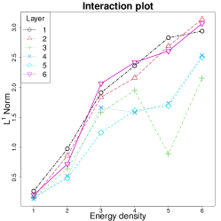
Figure 11: Interaction plot as a function of the energy density level and the layer in the real-case study.

Even if the use of RoFANOVA is recommended in light of the results shown by the Monte Carlo simulation study (Section 3), for the sake of completeness, the bi-dimensional version of the FNDP and TGPF test have been applied. For the latter, the Manly’s scheme (Manly, 2006) with 1000 random permutations was used to approximate the test statistic distribution. By comparing the additional results, which are shown in Table 2, with the proposed tests (Table 1) we note that they disagree in considering as significant the interaction between energy density and layer. In particular, the FNDP and the TGPF tests do not reject the null hypothesis of no interaction (i.e., large p-values). This may suggest, in accordance with the Monte Carlo simulation results achieved in the two-way FANOVA design case (Section 3.2), that FNDP and TGPF tests may have not enough statistical power to detect a technologically relevant interaction among the main factors.

Table 2: p-values of the FNDP and TGPF tests for $H_{0,Flu}$, $H_{0,Lay}$ and $H_{0,FluLay}$ against $H_{1,Flu}$, $H_{1,Lay}$ and $H_{1,FluLay}$.

	FNDP	TGPF
$H_{0,FluLay}$	0.72	0.23
$H_{0,Flu}$	0.00	0.00
$H_{0,Lay}$	0.00	0.00

5 Conclusion

In this paper, we have proposed the RoFANOVA test for the functional analysis of variance problem. In particular, the proposed method has been designed to be robust against functional outliers, which are increasingly common in complex problems and, as it is well known, can severely bias the analyses. Robustness comes from the use of robust test statistics based on the functional equivariant $M$-estimator and the functional normalized median absolute deviation, which are the extensions of the classical $M$-estimator and normalized median absolute deviation to functional data. The test statistic is, then, incorporated in a permutation test, in order to solve the FANOVA problem in a nonparametric fashion. The proposed approach is demonstrated to be flexible to different choices of the loss function, and, to be applicable to both one-dimensional and bi-dimensional functional data. To the best of the authors’ knowledge, this is the first example of a robust method for the FANOVA problem that is specifically designed to reduce the abnormal observation weights in the computation of the test statistic in comparisons with the standard least-squares loss function appeared in the literature, where attention has been mainly focused on non-robust methods.

The performance of the proposed method has been investigated by means of an extensive Monte Carlo simulation study, where the proposed RoFANOVA have been compared with other methods already present in the literature. The results have shown that the proposed tests clearly outperform the competitors in terms of both empirical size and empirical power when outlier contamination is present. Moreover, even in case of no outlier contamination the loss of power of the RoFANOVA tests with respect to competitors is negligible.

The proposed method was applied to a motivating real-case study in the field of additive manufacturing. Apart from the known influence of the energy density on the spatter intensity, in agreement with previous studies, the RoFANOVA test revealed a statistically significant interaction between the energy density and the laser scan direction relative to the shielding gas flow. The statistical significance of the interaction between these two factors was not identified by the other non-robust tests, which confirms the effectiveness of the proposed approach to applications where complex process dynamics may lead to outlying patterns that contaminate the experimental dataset. The validity of the proposed approach is naturally not limited to the case study here presented and, in general, to manufacturing applications.

In future research, the effects of heteroscedasticity on the RoFANOVA test should be investigated in order to be able to deal with a wider variety of settings. In addition, some efforts should be made to extend the proposed method to more complex FANOVA designs.

References

- Andani et al. (2017) Andani, M. T., R. Dehghani, M. R. Karamooz-Ravari, R. Mirzaeifar, and J. Ni (2017). Spatter formation in selective laser melting process using multi-laser technology. Materials & Design 131, 460–469.
- Anderson (2001) Anderson, M. J. (2001). Permutation tests for univariate or multivariate analysis of variance and regression. Canadian journal of fisheries and aquatic sciences 58(3), 626–639.
- Anwar and Pham (2018) Anwar, A. B. and Q.-C. Pham (2018). Study of the spatter distribution on the powder bed during selective laser melting. Additive Manufacturing 22, 86–97.
- Beaton and Tukey (1974) Beaton, A. E. and J. W. Tukey (1974). The fitting of power series, meaning polynomials, illustrated on band-spectroscopic data. Technometrics 16(2), 147–185.
- Bidare et al. (2018) Bidare, P., I. Bitharas, R. Ward, M. Attallah, and A. J. Moore (2018). Fluid and particle dynamics in laser powder bed fusion. Acta Materialia 142, 107–120.
- Bosq (2012) Bosq, D. (2012). Linear Processes in Function Spaces: Theory and Applications. Lecture Notes in Statistics. Springer New York.
- Brumback and Rice (1998) Brumback, B. A. and J. A. Rice (1998). Smoothing spline models for the analysis of nested and crossed samples of curves. Journal of the American Statistical Association 93(443), 961–976.
- Capezza et al. (2021) Capezza, C., F. Centofanti, A. Lepore, A. Menafoglio, B. Palumbo, and S. Vantini (2021). Functional regression control chart for monitoring ship CO2 emissions. Quality and Reliability Engineering International.
- Capezza et al. (2021) Capezza, C., F. Centofanti, A. Lepore, and B. Palumbo (2021). Functional clustering methods for resistance spot welding process data in the automotive industry. Applied Stochastic Models in Business and Industry 37(5), 908–925.
- Centofanti et al. (2021) Centofanti, F., A. Lepore, A. Menafoglio, B. Palumbo, and S. Vantini (2021). Functional regression control chart. Technometrics 63(3), 281–294.
- Colosimo et al. (2014) Colosimo, B., P. Cicorella, M. Pacella, and M. Blaco (2014). From profile to surface monitoring: Spc for cylindrical surfaces via gaussian processes. Journal of Quality Technology 46(2), 95–113.
- Colosimo et al. (2021) Colosimo, B., M. Grasso, F. Garghetti, and B. Rossi (2021). Complex geometries in additive manufacturing: A new solution for lattice structure modeling and monitoring. Journal of Quality Technology.
- Colosimo and Pacella (2010) Colosimo, B. and M. Pacella (2010). A comparison study of control charts for statistical monitoring of functional data. International Journal of Production Research 48(6), 1575–1601.
- Colosimo and Grasso (2020) Colosimo, B. M. and M. Grasso (2020). On-machine measurement, monitoring and control. Precision Metal Additive Manufacturing, 102.
- Colosimo et al. (2018) Colosimo, B. M., Q. Huang, T. Dasgupta, and F. Tsung (2018). Opportunities and challenges of quality engineering for additive manufacturing. Journal of Quality Technology 50(3), 233–252.
- Corain et al. (2014) Corain, L., V. B. Melas, A. Pepelyshev, and L. Salmaso (2014). New insights on permutation approach for hypothesis testing on functional data. Advances in Data Analysis and Classification 8(3), 339–356.
- Cuesta-Albertos and Febrero-Bande (2010) Cuesta-Albertos, J. and M. Febrero-Bande (2010). A simple multiway anova for functional data. Test 19(3), 537–557.
- Cuesta-Albertos and Fraiman (2006) Cuesta-Albertos, J. A. and R. Fraiman (2006). Impartial trimmed means for functional data. DIMACS Series in Discrete Mathematics and Theoretical Computer Science 72, 121.
- Cuesta-Albertos and Nieto-Reyes (2008) Cuesta-Albertos, J. A. and A. Nieto-Reyes (2008). The random tukey depth. Computational Statistics & Data Analysis 52(11), 4979–4988.
- Cuevas et al. (2004) Cuevas, A., M. Febrero, and R. Fraiman (2004). An anova test for functional data. Computational statistics & data analysis 47(1), 111–122.
- Cuevas and Fraiman (2009) Cuevas, A. and R. Fraiman (2009). On depth measures and dual statistics. a methodology for dealing with general data. Journal of Multivariate Analysis 100(4), 753–766.
- Everton et al. (2016) Everton, S. K., M. Hirsch, P. Stravroulakis, R. K. Leach, and A. T. Clare (2016). Review of in-situ process monitoring and in-situ metrology for metal additive manufacturing. Materials & Design 95, 431–445.
- Faraway (1997) Faraway, J. J. (1997). Regression analysis for a functional response. Technometrics 39(3), 254–261.
- Febrero-Bande and Oviedo de la Fuente (2012) Febrero-Bande, M. and M. Oviedo de la Fuente (2012). Statistical computing in functional data analysis: The R package fda.usc. Journal of Statistical Software 51(4), 1–28.
- Fraiman and Muniz (2001) Fraiman, R. and G. Muniz (2001). Trimmed means for functional data. Test 10(2), 419–440.
- Gibson et al. (2014) Gibson, I., D. Rosen, B. Stucker, and M. Khorasani (2014). Additive manufacturing technologies, Volume 17. Springer.
- Gonzalez and Manly (1998) Gonzalez, L. and B. F. Manly (1998). Analysis of variance by randomization with small data sets. Environmetrics: The official journal of the International Environmetrics Society 9(1), 53–65.
- Good (2013) Good, P. (2013). Permutation tests: a practical guide to resampling methods for testing hypotheses. Springer Science & Business Media.
- Górecki and Smaga (2015) Górecki, T. and Ł. Smaga (2015). A comparison of tests for the one-way anova problem for functional data. Computational Statistics 30(4), 987–1010.
- Gorecki and Smaga (2018) Gorecki, T. and L. Smaga (2018). fdanova: Analysis of variance for univariate and multivariate functional data. R package version 0.1.2.
- Grasso et al. (2014) Grasso, M., B. Colosimo, and M. Pacella (2014). Profile monitoring via sensor fusion: The use of pca methods for multi-channel data. International Journal of Production Research 52(20), 6110–6135.
- Grasso et al. (2017) Grasso, M., B. M. Colosimo, and F. Tsung (2017). A phase i multi-modelling approach for profile monitoring of signal data. International Journal of Production Research 55(15), 4354–4377.
- Grasso et al. (2021) Grasso, M., A. Remani, A. Dickins, B. Colosimo, and R. Leach (2021). In-situ measurement and monitoring methods for metal powder bed fusion: An updated review. Measurement Science and Technology 32(11).
- Gu (2013) Gu, C. (2013). Smoothing spline ANOVA models, Volume 297. Springer Science & Business Media.
- Guo (2002) Guo, W. (2002). Inference in smoothing spline analysis of variance. Journal of the Royal Statistical Society: Series B (Statistical Methodology) 64(4), 887–898.
- Guo et al. (2019) Guo, W., J. Jin, and S. Jack Hu (2019). Profile monitoring and fault diagnosis via sensor fusion for ultrasonic welding. Journal of Manufacturing Science and Engineering, Transactions of the ASME 141(8).
- Hampel (1974) Hampel, F. R. (1974). The influence curve and its role in robust estimation. Journal of the american statistical association 69(346), 383–393.
- Hampel et al. (2011) Hampel, F. R., E. M. Ronchetti, P. J. Rousseeuw, and W. A. Stahel (2011). Robust statistics: the approach based on influence functions, Volume 196. John Wiley & Sons.
- Horváth and Kokoszka (2012) Horváth, L. and P. Kokoszka (2012). Inference for functional data with applications. Springer Science & Business Media.
- Hsing and Eubank (2015) Hsing, T. and R. Eubank (2015). Theoretical foundations of functional data analysis, with an introduction to linear operators. John Wiley & Sons.
- Huber (2004) Huber, P. J. (2004). Robust statistics, Volume 523. John Wiley & Sons.
- Huber et al. (1964) Huber, P. J. et al. (1964). Robust estimation of a location parameter. The Annals of Mathematical Statistics 35(1), 73–101.
- Hubert et al. (2015) Hubert, M., P. J. Rousseeuw, and P. Segaert (2015). Multivariate functional outlier detection. Statistical Methods & Applications 24(2), 177–202.
- Kalogridis and Van Aelst (2019) Kalogridis, I. and S. Van Aelst (2019). Robust functional regression based on principal components. Journal of Multivariate Analysis 173, 393–415.
- Kokoszka and Reimherr (2017) Kokoszka, P. and M. Reimherr (2017). Introduction to functional data analysis. CRC Press.
- Lehmann and Romano (2006) Lehmann, E. L. and J. P. Romano (2006). Testing statistical hypotheses. Springer Science & Business Media.
- López-Pintado and Romo (2009) López-Pintado, S. and J. Romo (2009). On the concept of depth for functional data. Journal of the American Statistical Association 104(486), 718–734.
- López-Pintado and Romo (2011) López-Pintado, S. and J. Romo (2011). A half-region depth for functional data. Computational Statistics & Data Analysis 55(4), 1679–1695.
- Ly et al. (2017) Ly, S., A. M. Rubenchik, S. A. Khairallah, G. Guss, and M. J. Matthews (2017). Metal vapor micro-jet controls material redistribution in laser powder bed fusion additive manufacturing. Scientific reports 7(1), 1–12.
- Manly (2006) Manly, B. F. (2006). Randomization, bootstrap and Monte Carlo methods in biology, Volume 70. CRC press.
- Maronna et al. (2019) Maronna, R. A., R. D. Martin, V. J. Yohai, and M. Salibián-Barrera (2019). Robust statistics: theory and methods (with R). John Wiley & Sons.
- Megahed et al. (2011) Megahed, F., W. Woodall, and J. Camelio (2011). A review and perspective on control charting with image data. Journal of Quality Technology 43(2), 83–98.
- Menafoglio et al. (2018) Menafoglio, A., M. Grasso, P. Secchi, and B. Colosimo (2018). Profile monitoring of probability density functions via simplicial functional pca with application to image data. Technometrics 60(4), 497–510.
- Miller Jr (1997) Miller Jr, R. G. (1997). Beyond ANOVA: basics of applied statistics. CRC press.
- Montgomery (2017) Montgomery, D. C. (2017). Design and analysis of experiments. John wiley & sons.
- Noorossana and Amiri (2011) Noorossana, Rassoul, S. A. and A. Amiri (2011). Statistical analysis of profile monitoring.
- Paynabar et al. (2013) Paynabar, K., J. Jin, and M. Pacella (2013). Monitoring and diagnosis of multichannel nonlinear profile variations using uncorrelated multilinear principal component analysis. IIE Transactions (Institute of Industrial Engineers) 45(11), 1235–1247.
- Pesarin and Salmaso (2010) Pesarin, F. and L. Salmaso (2010). Permutation tests for complex data: theory, applications and software. John Wiley & Sons.
- Pini and Vantini (2017) Pini, A. and S. Vantini (2017). Interval-wise testing for functional data. Journal of Nonparametric Statistics 29(2), 407–424.
- Pini et al. (2018) Pini, A., S. Vantini, B. M. Colosimo, and M. Grasso (2018). Domain-selective functional analysis of variance for supervised statistical profile monitoring of signal data. Journal of the Royal Statistical Society: Series C (Applied Statistics) 67(1), 55–81.
- Qiu et al. (2010) Qiu, P., C. Zou, and Z. Wang (2010). Nonparametric profile monitoring by mixed effects modeling. Technometrics 52(3), 265–277.
- R Core Team (2020) R Core Team (2020). R: A Language and Environment for Statistical Computing. Vienna, Austria: R Foundation for Statistical Computing.
- Ramsay (2005) Ramsay, J. O. (2005). Functional data analysis. Wiley Online Library.
- Repossini et al. (2017) Repossini, G., V. Laguzza, M. Grasso, and B. M. Colosimo (2017). On the use of spatter signature for in-situ monitoring of laser powder bed fusion. Additive Manufacturing 16, 35–48.
- Schrader and Hettmansperger (1980) Schrader, R. M. and T. P. Hettmansperger (1980). Robust analysis of variance based upon a likelihood ratio criterion. Biometrika 67(1), 93–101.
- Schrader and Mc Kean (1977) Schrader, R. M. and J. W. Mc Kean (1977). Robust analysis of variance. Communications in Statistics-Theory and Methods 6(9), 879–894.
- Shen and Faraway (2004) Shen, Q. and J. Faraway (2004). An f test for linear models with functional responses. Statistica Sinica, 1239–1257.
- Sinova et al. (2018) Sinova, B., G. Gonzalez-Rodriguez, S. Van Aelst, et al. (2018). M-estimators of location for functional data. Bernoulli 24(3), 2328–2357.
- Wang and Tsung (2005) Wang, K. and F. Tsung (2005). Using profile monitoring techniques for a data-rich environment with huge sample size. Quality and Reliability Engineering International 21(7), 677–688.
- Wells et al. (2013) Wells, L., F. Megahed, C. Niziolek, J. Camelio, and W. Woodall (2013). Statistical process monitoring approach for high-density point clouds. Journal of Intelligent Manufacturing 24(6), 1267–1279.
- Wood (2017) Wood, S. N. (2017). Generalized additive models: an introduction with R. CRC press.
- Yang et al. (2020) Yang, L., L. Lo, S. Ding, and T. Özel (2020). Monitoring and detection of meltpool and spatter regions in laser powder bed fusion of super alloy inconel 625. Progress in Additive Manufacturing 5(4), 367–378.
- Young et al. (2020) Young, Z. A., Q. Guo, N. D. Parab, C. Zhao, M. Qu, L. I. Escano, K. Fezzaa, W. Everhart, T. Sun, and L. Chen (2020). Types of spatter and their features and formation mechanisms in laser powder bed fusion additive manufacturing process. Additive Manufacturing 36, 101438.
- Zang and Qiu (2018) Zang, Y. and P. Qiu (2018). Phase ii monitoring of free-form surfaces: An application to 3d printing. Journal of Quality Technology 50(4), 379–390.
- Zhang (2011) Zhang, J.-T. (2011). Statistical inferences for linear models with functional responses. Statistica Sinica, 1431–1451.
- Zhang (2013) Zhang, J.-T. (2013). Analysis of variance for functional data. CRC Press.
- Zhang et al. (2007) Zhang, J.-T., J. Chen, et al. (2007). Statistical inferences for functional data. The Annals of Statistics 35(3), 1052–1079.
- Zhang and Liang (2014) Zhang, J.-T. and X. Liang (2014). One-way anova for functional data via globalizing the pointwise f-test. Scandinavian Journal of Statistics 41(1), 51–71.