Regularity based spectral clustering and mapping the Fiedler-carpet

Abstract

Spectral clustering is discussed from many perspectives, by extending it to rectangular arrays and discrepancy minimization too. Near optimal clusters are obtained with singular value decomposition and with the weighted $k$-means algorithm. In case of rectangular arrays, this means enhancing the method of correspondence analysis with clustering, and in case of edge-weighted graphs, a normalized Laplacian based clustering. In the latter case it is proved that a spectral gap between the $(k-1)$th and $k$th smallest positive eigenvalues of the normalized Laplacian matrix gives rise to a sudden decrease of the inner cluster variances when the number of clusters of the vertex representatives is $2^{k-1}$, but only the first $k-1$ eigenvectors, constituting the so-called Fiedler-carpet, are used in the representation. Application to directed migration graphs is also discussed.

Keywords: multiway discrepancy, correspondence analysis, normalized Laplacian, multiway cuts, Fiedler-vector, weighted $k$-means algorithm.

MSC2020: 05C50,62H25,65H10.

1 Introduction

Spectral graph theory started developing about 50 years ago (see, e.g. A.J. Hoffman [15], M. Fiedler [14], D.M. Cvetković [12], and F. Chung [10]) to characterize certain structural properties of a graph by means of the eigenvalues of its adjacency or Laplacian matrix. Later on, in the last decades of the 20th century, the eigenvectors corresponding to some near zero eigenvalues of the Laplacian matrix were also used for clustering the vertices into disjoint parts so that the inter-cluster relations are negligible compared to the intra-cluster ones (usual purpose of cluster analysis as a machine learning technique). In this setup, the famous Fiedler-vector, the eigenvector, corresponding to the smallest positive Laplacian eigenvalue was used to classify the vertices into two parts; while later, $k$ eigenvectors ($k\geq 2$) entered into the $k$-clustering task. It was also noted in [2] that the more eigenvectors, the better, but not exact estimates between the spectral gap and the quality of the clustering were available, except the $k=1$ and $k=2$ cases; former related to the isoperimetric number and expander graphs (see e.g. [19, 10, 16]) and latter to the sum of the inner variances of 2-clusterings (see [3]).

Since then, the problem was generalized in several ways: to edge-weighted graphs and rectangular arrays of nonnegative entries (e.g. microarrays in biological genetics and forensic science [4, 7, 9, 17]), and to degree-corrected adjacency and Laplacian matrices [6, 11]. After the millennium, physicists and social scientists introduced modularity matrices and investigated so-called anti-community structures (intra-cluster relations are negligible compared to the inter-cluster ones) in contrast to the former community structures [20]. By uniting these two approaches, so-called regular cluster pairs with small discrepancy can be defined, where homogeneous clusters are looked for (e.g. in microarrays one looks for groups of genes that similarly influence the same groups of conditions) [7]. The existence of such a regular structure is theoretically guaranteed by the Abel-prize winner Szemeredi’s regularity lemma [24] that for any small positive $\varepsilon$ guarantees a universal number $k$ of clusters (irrespective of the numbers of vertices) such that partitioning the vertices into $k$ parts (and possibly a small exceptional one), the pairs have discrepancy less than $\varepsilon$. However, this $k$ can be enormously large and not applicable to practical purposes. Our purpose is to give a moderate $k$ where the sum of the inner variances of $2^{k-1}$ clusters is estimated from above by the spectral gap between the $(k-1)$th and $k$th positive normalized Laplacian eigenvalues in their non-decreasing order, even in the worst case scenario. This is the generalization of a theorem of [3] that was applicable only to the $k=2$ situation. There $2^{k-1}$ and $k$ were the same, and the Fiedler-vector was used for clustering into $k=2$ parts. If $k>2$, then we use $k-1$ non-trivial eigenvectors that form what we call Fiedler-carpet. In special cases, e.g. in case of generalized multiclass random or quasirandom graphs, both the objective function of the $k$-means algorithm and the the $k$-way discrepancy dramatically decreases compared to the $k-1$ one [8], where the number of clusters is one more than the number of eigenvectors used in the representation. However, in the generic case, the number of eigenvectors entered into the classification is much less than the number of clusters, that is also a good news from the point of view of computational complexity.

The organization of the paper is as follows. In Section 2, the most important notions and facts are defined, concerning normalized Laplacian spectra and multiway discrepancy of rectangular arrays with nonnegative entries [1, 6, 7, 8, 9]. In Section 3, the main theorem is stated and proved. The proof is based on the energy minimizing representation and analyzing the structure of the vertex representatives and the underlying spectral subspaces that are mapped in a convenient way. In Appendix A, next to technical considerations, simulation results, and plots of the so-obtained Fiedler-carpet are also presented. Real-life application to the directed graph of migration data is discussed in Section 4, supplemented with more figures in Appendix B. In Section 5, the main contributions are summarized and conclusions are drawn.

2 Minimal and regular cuts versus spectra

Let $\bm{W}$ be the $n\times n$ edge-weight matrix of a graph $G$ on $n$ vertices. It is symmetric, has 0 diagonal and nonnegative entries. In case of a simple graph, $\bm{W}=(w_{ij})$ is the usual adjacency matrix. The generalized degrees are $d_{i}=\sum_{j=1}^{n}w_{ij}$, for $i=1,\dots,n$. Assume that $d_{i}$s are all positive and the diagonal degree-matrix $\bm{D}$ contains them in its main diagonal. The Laplacian of $G$ is $\bm{L}=\bm{D}-\bm{W}$, while its normalized Laplacian is

$$\bm{L}_{\bm{D}}=\bm{I}-\bm{D}^{-1/2}\bm{W}\bm{D}^{-1/2}.$$

Because of the normalization, $\bm{L}_{\bm{D}}$ is not affected by the scaling of the edge-weights, therefore $\sum_{i=1}^{n}d_{i}=1$ can be assumed. $\bm{L}_{\bm{D}}$ is positive semidefinite, and if $\bm{W}$ is irreducible ($G$ is connected), then its eigenvalues are

$$0=\lambda_{0}<\lambda_{1}\leq\dots\leq\lambda_{n-1}\leq 2$$

with unit-norm pairwise orthogonal eigenvectors $\mathbf{u}_{0},\mathbf{u}_{1},\dots,\mathbf{u}_{n-1}$. In particular, $\mathbf{u}_{0}=(\sqrt{d_{1}},\dots,\sqrt{d_{n}})^{T}=:\sqrt{\mathbf{d}}^{T}$.

For $1<d<n$, the row vectors of the $n\times d$ matrix $\bm{X}^{*}=(\bm{D}^{-1/2}\mathbf{u}_{1},\dots,\bm{D}^{-1/2}\mathbf{u}_{d})$ are optimal $d$-dimensional representatives $\mathbf{r}^{*}_{1},\dots,\mathbf{r}^{*}_{n}$ of the vertices that minimize the energy function

$$Q_{d}(\bm{X})=\sum_{i=1}^{n-1}\sum_{j=i+1}^{n}w_{ij}\|\mathbf{r}_{i}-\mathbf{r}_{j}\|^{2}=\mathrm{tr}(\bm{X}^{T}\bm{L}\bm{X}),$$ (1)

where the general vertex-representatives $\mathbf{r}_{1},\dots,\mathbf{r}_{n}\in\mathbb{R}^{d}$ are row vectors of the $n\times d$ matrix $\bm{D}^{-1/2}\bm{X}$. They satisfy the constraints $\bm{X}^{T}\bm{D}\bm{X}=\bm{I}_{d}$ and $\sum_{i=1}^{n}d_{i}\mathbf{r}_{i}=\mathbf{0}$. Minimizing the energy $Q_{d}(\bm{X})$ supports representatives of vertices connected with large weights to be close to each other. The minimum of $Q_{d}(\bm{X})$ is the sum of the $d$ smallest positive eigenvalues of $\bm{L}_{\bm{D}}$.

The weighted k-variance of these representatives is defined as

$${S}_{k}^{2}(\bm{X})=\min_{(V_{1},\dots,V_{k})\in{\cal P}_{k}}\sum_{i=1}^{k}\sum_{j\in V_{i}}d_{j}\|\mathbf{r}_{j}-{\mathbf{c}}_{i}\|^{2},$$ (2)

where ${\mathrm{Vol}}(U)=\sum_{j\in U}d_{j}$, ${\mathbf{c}}_{i}=\frac{1}{{\mathrm{Vol}}(V_{i})}\sum_{j\in V_{i}}d_{j}\mathbf{r}_{j}$ is the weighted center of the cluster $V_{i}$, and the minimization is over proper $k$-partitions $P_{k}=(V_{1},\dots,V_{k})$ of the vertex-set, their collection is denoted by ${\cal P}_{k}$.

It is the weighted $k$-means algorithm that approaches this minimum. In [22], it is stated that if the data satisfy the $k$-clusterable criterion ($S_{k}^{2}\leq\epsilon^{2}S_{k-1}^{2}$ with a small enough $\epsilon$), then there is a PTAS (polynomial time approximation scheme) for the $k$-means problem. This is the situation we usually owe.

It is well known that the $k$ bottom eigenvalues of the normalized Laplacian matrix estimate the $k$-way normalized cut of $G$ which is $f_{k}(G)=\min_{P_{k}\in{\cal P}_{k}}f(P_{k},G)$, where

$$f(P_{k},G) =\sum_{a=1}^{k-1}\sum_{b=a+1}^{k}\left(\frac{1}{{\mathrm{Vol}}(V_{a})}+\frac{1}{{\mathrm{Vol}}(V_{b})}\right)w(V_{a},V_{b})$$

$$=\sum_{a=1}^{k}\frac{w(V_{a},{\overline{V}}_{a})}{{\mathrm{Vol}}(V_{a})}=k-\sum_{a=1}^{k}\frac{w(V_{a},V_{a})}{{\mathrm{Vol}}(V_{a})}.$$

Here $w(V_{a},V_{b})=\sum_{i\in V_{a}}\sum_{j\in V_{b}}w_{ij}$ is the weighted cut between the cluster pairs. Since $\sum_{i=1}^{k-1}\lambda_{i}$ is the overall minimum of $Q_{k}$ (on the orthogonality constraints) and $f_{k}(G)$ is the minimum over partition vectors (having stepwise constant coordinates over the parts of $P_{k}$), the relation

$$\sum_{i=1}^{k-1}\lambda_{i}\leq f_{k}(G)$$ (3)

is easy to prove. This estimate is sharper if the eigensubspace spanned by the corresponding eigenvectors is closer to that of the partition vectors in the convenient $k$-partition of the vertices, the one produced by the weighted k-means algorithm. Therefore $S_{k}^{2}(\bm{X}_{k-1}^{*})$ indicates the quality of the $k$-clustering based on the $k-1$ bottom eigenvectors (except the trivial one). Later it will be used that neither $Q_{k}$ nor $S_{k}^{2}(\bm{X}_{k-1}^{*})$ is affected by the orientation of the orthonormal eigenvectors.

In [3] it is proved that $S_{2}^{2}(\bm{X}_{1}^{*})\leq\frac{\lambda_{1}}{\lambda_{2}}$, so the larger the gap after the first positive eigenvalue of $\bm{L}_{\bm{D}}$, the sharper the estimate in (3) is. Here this statement is generalized to the gap between $\lambda_{k-1}$ and $\lambda_{k}$, but $2^{k-1}$ clusters are considered based on $(k-1)$-dimensional vertex representatives. In the literature (see, e.g. [18, 21, 23]) the number of clusters is usually the same as the number of eigenvectors entered into the classification. The message of Theorem 1 of Section 3 is that the number of clusters is much higher in the generic case than the dimension of the representatives, at least in the minimum multiway cut problems. Though, with discrepancy objective, the famous Szemerédi Regularity Lemma [24] also suggests this.

Now consider the discrepancy view and the related matrices. The whole can better be illustrate on rectangular arrays of nonnegative entries; simple, edge-weighted, and directed graphs are special cases.

In many applications, for example when microarrays are analyzed, our data are collected in the form of an $m\times n$ rectangular matrix $\bm{C}=(c_{ij})$ of nonnegative real entries. (If the entries are integer frequency counts, then the array is called contingency table in statistics.) We assume that $\bm{C}$ is non-degenerate, i.e. $\bm{C}\bm{C}^{T}$ (when $m\leq n$) or $\bm{C}^{T}\bm{C}$ (when $m>n$) is irreducible. Consequently, the row-sums $d_{row,i}=\sum_{j=1}^{n}c_{ij}$ and column-sums $d_{col,j}=\sum_{i=1}^{m}c_{ij}$ of $\bm{C}$ are strictly positive, and the diagonal matrices $\bm{D}_{row}=\mathrm{diag}(d_{row,1},\dots,d_{row,m})$ and $\bm{D}_{col}=\mathrm{diag}(d_{col,1},\dots,d_{col,n})$ are regular. Without loss of generality, we also assume that $\sum_{i=1}^{n}\sum_{j=1}^{m}c_{ij}=1$, since neither our main object, the normalized contingency table

$$\bm{C}_{\bm{D}}=\bm{D}_{row}^{-1/2}\bm{C}\bm{D}_{col}^{-1/2},$$ (4)

nor the multiway discrepancies to be introduced are affected by the scaling of the entries of $\bm{C}$. It is known that the singular values of $\bm{C}_{D}$ are in the [0,1] interval. The positive ones, enumerated in non-increasing order, are the real numbers

$$1=s_{0}>s_{1}\geq\dots\geq s_{r-1}>0,$$

where $r=\mathrm{rank}(\bm{C}_{D})=\mathrm{rank}(\bm{C})$. Provided $\bm{C}$ is non-degenerate, 1 is a single singular value; it will be called trivial and denoted by $s_{0}$, since it corresponds to the trivial singular vector pair, which are disregarded in the clustering problems. This is a well-known fact of correspondence analysis, for further explanation see [6, 13] and the subsequent paragraph.

For a given integer $1\leq k\leq\min\{m,n\}$, we are looking for $k$-dimensional representatives $\mathbf{r}_{1},\dots,\mathbf{r}_{m}\in\mathbb{R}^{k}$ of the rows and $\mathbf{q}_{1},\dots,\mathbf{q}_{n}\in\mathbb{R}^{k}$ of the columns such that they minimize the energy function

$$Q_{k}=\sum_{i=1}^{m}\sum_{j=1}^{n}c_{ij}\|\mathbf{r}_{i}-\mathbf{q}_{j}\|^{2}$$ (5)

subject to

$$\sum_{i=1}^{m}d_{row,i}\mathbf{r}_{i}\mathbf{r}_{i}^{T}=\bm{I}_{k}\quad\textrm{and}\quad\sum_{j=1}^{n}d_{col,j}\mathbf{q}_{j}\mathbf{q}_{j}^{T}=\bm{I}_{k}.$$ (6)

When minimized, the objective function $Q_{k}$ favors $k$-dimensional placement of the rows and columns such that representatives of columns and rows with large association are forced to be close to each other. It is easy to prove that the minimum is obtained by the singular value decomposition (SVD)

$$\bm{C}_{\bm{D}}=\sum_{k=0}^{r-1}s_{k}\mathbf{v}_{k}\mathbf{u}_{k}^{T},$$ (7)

where $r\leq\min\{n,m\}$ is the rank of $\bm{C}_{\bm{D}}$. The constrained minimum of $Q_{k}$ is $2k-\sum_{i=0}^{k-1}s_{i}$ and it is attained with row- and column-representatives that are row vectors of the matrices $\bm{D}_{row}^{-1/2}(\mathbf{v}_{0},\mathbf{v}_{1},\dots,\mathbf{v}_{k-1})$ and $\bm{D}_{col}^{-1/2}(\mathbf{u}_{0},\mathbf{u}_{1},\dots,\mathbf{u}_{k-1})$, respectively.

Note that if the entries of $\bm{C}$ are frequency counts and their sum ($N$) is the sample size, then the $\chi^{2}$ statistic, which measures the deviation from independence, is

$$\chi^{2}=N\sum_{i=1}^{r-1}s_{i}^{2}.$$ (8)

If the $\chi^{2}$ test based on this statistic indicates significant deviance from independence (i.e. from the rank 1 approximation of $\bm{C}$), then one may look for rank $k$ approximation $(1<k<r=\mathrm{rank})$, which is constructed by the first $k$ singular vector pairs.

With bi-clustering the rows and columns of $\bm{C}$ one also may look for sub-tables close to independent ones. This is measured by the discrepancy. In [7], the multiway discrepancy of the rectangular matrix $\bm{C}$ of nonnegative entries in the proper $k$-partition $R_{1},\dots,R_{k}$ of its rows and $C_{1},\dots,C_{k}$ of its columns is defined as

$$\mathrm{md}(\bm{C};R_{1},\dots,R_{k},C_{1},\dots,C_{k}) =\max_{\begin{subarray}{c}1\leq a,b\leq k\\ X\subset R_{a},\,Y\subset C_{b}\end{subarray}}\frac{|c(X,Y)-\rho(R_{a},C_{b}){\mathrm{Vol}}(X){\mathrm{Vol}}(Y)|}{\sqrt{{\mathrm{Vol}}(X){\mathrm{Vol}}(Y)}}$$ (9)

$$=|\rho(X,Y)-\rho(R_{a},C_{b})|{\sqrt{{\mathrm{Vol}}(X){\mathrm{Vol}}(Y)}}$$

where $c(X,Y)=\sum_{i\in X}\sum_{j\in Y}c_{ij}$ is the cut between $X\subset R_{a}$ and $Y\subset C_{b}$, ${\mathrm{Vol}}(X)=\sum_{i\in X}d_{row,i}$ is the volume of the row-subset $X$, ${\mathrm{Vol}}(Y)=\sum_{j\in Y}d_{col,j}$ is the volume of the column-subset $Y$, whereas $\rho(R_{a},C_{b})=\frac{c(R_{a},C_{b})}{{\mathrm{Vol}}(R_{a}){\mathrm{Vol}}(C_{b})}$ denotes the relative density between $R_{a}$ and $C_{b}$. The minimum $k$-way discrepancy of $\bm{C}$ itself is

$$\mathrm{md}_{k}(\bm{C})=\min_{\begin{subarray}{c}R_{1},\dots,R_{k}\\ C_{1},\dots,C_{k}\end{subarray}}\mathrm{md}(\bm{C};R_{1},\dots,R_{k},C_{1},\dots,C_{k}).$$

In [7] the following is proved:

$$s_{k}\leq 9\mathrm{md}_{k}(\bm{C})(k+2-9k\ln\mathrm{md}_{k}(\bm{C})),$$

provided $0<\mathrm{md}_{k}(\bm{C})<1$. In the forward direction, the following is established in [6]. Given the $m\times n$ contingency table $\bm{C}$, consider the spectral clusters $R_{1},\dots,R_{k}$ of its rows and $C_{1},\dots,C_{k}$ of its columns, obtained by applying the weighted $k$-means algorithm to the $(k-1)$-dimensional row- and column representatives. Let $S_{k,row}^{2}$ and $S_{k,col}^{2}$ denote the minima of the $k$-means algorithm with them, respectively. Then, under some balancing conditions for the margins and for the cluster sizes, $\mathrm{md}_{k}(\bm{C})\leq B(\sqrt{2k}(S_{k,row}+S_{k,col})+s_{k})$, with some constant $B$, which depends only on the constants of the balancing conditions, and does not depend on $m$ and $n$. Roughly speaking, the two directions together imply that if $s_{k}$ is ‘small’ and ‘much smaller’ than $s_{k-1}$, then one may expect a simultaneous $k$-clustering of the rows and columns of $\bm{C}$ with small $k$-way discrepancy. This is the case of generalized random and quasirandom graphs [8].

This notion can be extended to an edge-weighted graph $G$ and denoted by $\mathrm{md}_{k}(G)$. In that setup, $\bm{C}$ plays the role of the weighted adjacency matrix (symmetric in the undirected; quadratic, but usually not symmetric in the directed case). Here the singular values of the normalized adjacency matrix are the absolute values of the eigenvalues, which enter into the estimates, in decreasing order.

At this point, some new matrices are introduced, originally defined by physicists (see [20]). The modularity matrix of an edge-weighted graph $G$ is defined as $\bm{M}=\bm{W}-\mathbf{d}\mathbf{d}^{T}$, where the entries of $\bm{W}$ sum to 1. The normalized modularity matrix of $G$ (see [5]) is

$$\bm{M}_{\bm{D}}=\bm{D}^{-1/2}\bm{M}\bm{D}^{-1/2}=\bm{D}^{-1/2}\bm{W}\bm{D}^{-1/2}-\sqrt{\mathbf{d}}\sqrt{\mathbf{d}}^{T}=\bm{W}_{\bm{D}}-\sqrt{\mathbf{d}}\sqrt{\mathbf{d}}^{T}.$$

The normalized modularity matrix is the normalized edge-weight matrix deprived of the trivial dyad. Obviously, $\bm{L}_{\bm{D}}=\bm{I}-\bm{W}_{\bm{D}}=\bm{I}-\bm{M}_{\bm{D}}-\sqrt{\mathbf{d}}\sqrt{\mathbf{d}}^{T}$, see [6].

Therefore, the $k-1$ largest singular values of $\bm{M}_{\bm{D}}$ are the absolute values of the $k-1$ largest eigenvalues of $\bm{W}_{\bm{D}}$ (except the trivial 1). These, in turn, are 1 minus the $k-1$ positive eigenvalues of $\bm{L}_{\bm{D}}$ which are in the farthest distance from 1. If those are all less then 1, then these are $1-\lambda_{1},\dots,1-\lambda_{k-1}$. In this case, the regularity based spectral clustering boils down to the minimum cut objective.

Otherwise, for a $1<k<n$ fixed integer, in the modularity based spectral clustering, we look for the proper $k$-partition $V_{1},\dots,V_{k}$ of the vertices such that the within- and between cluster discrepancies are minimized. To motivate the introduction of the exact discrepancy measure observe that the $ij$ entry of $\bm{M}$ is $w_{ij}-d_{i}d_{j}$, which is the difference between the actual connection of the vertices $i,j$ and the connection that is expected under independent attachment of them with probabilities $d_{i}$ and $d_{j}$, respectively. Consequently, the difference between the actual and the expected connectedness of the subsets $X,Y\subset V$ is

$$\sum_{i\in X}\sum_{j\in Y}(w_{ij}-d_{i}d_{j})=w(X,Y)-{\mathrm{Vol}}(X){\mathrm{Vol}}(Y).$$

A directed edge-weighted graph $G=(V,\bm{W})$ is described by its quadratic, but usually not symmetric weighted adjacency matrix $\bm{W}=(w_{ij})$ of zero diagonal, where $w_{ij}$ is the nonnegative weight of the $j\to i$ edge $(i\neq j)$. The row-sums $d_{in,i}=\sum_{j=1}^{n}w_{ij}$ and column-sums $d_{out,j}=\sum_{i=1}^{n}w_{ij}$ of $\bm{W}$ are the in- and out-degrees, while $\bm{D}_{in}=\mathrm{diag}(d_{in,1},\dots,d_{in,n})$ and $\bm{D}_{out}=\mathrm{diag}(d_{out,1},\dots,d_{out,n})$ are the diagonal in- and out-degree matrices. The multiway discrepancy of the directed, edge-weighted graph $G=(V,\bm{W})$ in the in-clustering $V_{in,1},\dots,V_{in,k}$ and out-clustering $V_{out,1},\dots,V_{out,k}$ of its vertices is

$$\mathrm{md}(G;V_{in,1},\dots,V_{in,k},V_{out,1},\dots,V_{out,k})$$

$$=\max_{\begin{subarray}{c}1\leq a,b\leq k\\ X\subset V_{out,a},\,Y\subset V_{in,b}\end{subarray}}\frac{|w(X,Y)-\rho(V_{out,b},V_{in,a}){\mathrm{Vol}}_{in}(X){\mathrm{Vol}}_{out}(Y)|}{\sqrt{{\mathrm{Vol}}_{n}(X){\mathrm{Vol}}_{out}(Y)}},$$

where $w(X,Y)$ is the sum of the weights of the $X\to Y$ edges, whereas ${\mathrm{Vol}}_{in}(X)=\sum_{i\in X}d_{in,i}$ and ${\mathrm{Vol}}_{out}(Y)=\sum_{j\in Y}d_{out,j}$ are the out- and in-volumes, respectively. The minimum $k$-way discrepancy of the directed edge-weighted graph $G=(V,\bm{W})$ is

$$\mathrm{md}_{k}(G)=\min_{\begin{subarray}{c}V_{in,1},\dots,V_{in,k}\\ V_{out,1},\dots,V_{out,k}\end{subarray}}\mathrm{md}(G;V_{in,1},\dots,V_{in,k},V_{out,1},\dots,V_{out,k}).$$

In [7] it is proved that

$$s_{k}\leq 9\mathrm{md}_{k}(G)(k+2-9k\ln\mathrm{md}_{k}(G)),$$

where $s_{k}$ is the $k$-th largest nontrivial singular value of the normalized weighted adjacency matrix $\bm{W}_{\bm{D}}=\bm{D}_{in}^{-1/2}\bm{W}\bm{D}_{out}^{-1/2}$. In Section 4 we apply the SVD of $\bm{W}_{\bm{D}}$ to find migration patterns, i.e. emigration and immigration trait clusters.

3 Mapping the Fiedler-carpet: more clusters than eigenvectors

Theorem 1.

Let $G=(V,\bm{W})$ be connected edge-weighted graph with generalized degrees $d_{1},\dots,d_{n}$ and assume that $\sum_{i=1}^{n}d_{i}=1$. Let $0=\lambda_{0}<\lambda_{1}\leq\dots\leq\lambda_{n-1}\leq 2$ denote the eigenvalues of the normalized Laplacian matrix $\bm{L}_{\bm{D}}$ of $G$. Then for the weighted $2^{k-1}$-variance of the optimal $(k-1)$-dimensional vertex representatives, comprising row vectors of the matrix $\bm{X}_{k-1}^{*}$, the following upper estimate holds:

$${S}_{2^{k-1}}^{2}(\bm{X}_{k-1}^{*})\leq\dfrac{\sum_{j=1}^{k-1}\lambda_{j}}{\lambda_{k}},$$

provided $\lambda_{k-1}<\lambda_{k}$.

Proof.

Recall that, with the notation of Section 2, $\bm{X}_{k-1}^{*}=(\bm{D}^{-1/2}\mathbf{u}_{1},\dots,\bm{D}^{-1/2}\mathbf{u}_{k-1})$, where the trivial $\bm{D}^{-1/2}\mathbf{u}_{0}=\mathbf{1}$ vector is disregarded, and $\mathbf{u}_{0},\mathbf{u}_{1},\dots\mathbf{u}_{k-1}$ are unit-norm, pairwise orthogonal eigenvectors corresponding to the eigenvalues $0=\lambda_{0}<\lambda_{1}\leq\dots\leq\lambda_{k-1}$ of $\bm{L}_{D}$, respectively. As the trivial dimension is disregarded, we only use the coordinates of the vectors $\mathbf{x}_{j}:=\bm{D}^{-1/2}\mathbf{u}_{j}=(x_{j1},\dots,x_{jn})^{T}$ for $j=1,\dots,k-1$.

Since $\mathbf{u}_{1},\dots\mathbf{u}_{k-1}$ form an orthonormal set and they are orthogonal to the $\mathbf{u}_{0}=\sqrt{\mathbf{d}}$ vector, for the coordinates of $\mathbf{x}_{j}$ the following relations hold:

$$\sum_{i=1}^{n}d_{i}x_{ji}=0,\,\sum_{i=1}^{n}d_{i}x_{ji}^{2}=1\,(j=1,\dots,k-1),\,\sum_{i=1}^{n}d_{i}x_{ji}x_{li}=0\,(j\neq l).$$ (10)

Now we will find a vector $\mathbf{y}=(y_{1},\dots,y_{n})^{T}$ such that for it, the conditions

$$\sum_{i=1}^{n}d_{i}y_{i}=0$$ (11)

and

$$\sum_{i=1}^{n}d_{i}x_{ji}y_{i}=0,\quad j=1,\dots,k-1$$ (12)

hold. We are looking for $\mathbf{y}$ in the following form:

$$y_{i}:=\sum_{j=1}^{k-1}|x_{ji}-a_{j}|-b,\quad i=1,\dots,n,$$ (13)

where $a_{1},\dots,a_{k-1}$ and $b$ are appropriate real numbers. We will show that there exist such real numbers that $y_{i}$’s defined by them satisfy conditions (11) and (12).

Indeed, when we already have $a_{1},\dots,a_{k-1}$, the above conditions together with $\sum_{i=1}^{n}d_{i}=1$ yield

$$b=\sum_{j=1}^{k-1}b_{j},\quad b_{j}=\sum_{i=1}^{n}d_{i}|x_{ji}-a_{j}|,\quad j=1,\dots,k-1.$$ (14)

With this choice of $b$, the fulfillment of (12) means that for $j=1,\dots,k-1$:

$$\sum_{i=1}^{n}d_{i}x_{ji}y_{i}=\sum_{i=1}^{n}d_{i}x_{ji}\left(\sum_{l=1}^{k-1}|x_{li}-a_{l}|-b_{l}\right)=0.$$

But (10) implies that

$$\sum_{i=1}^{n}d_{i}x_{ji}b_{l}=0$$

for $l=1,\dots,k-1$. This provides the following system of equations for $a_{1},\dots,a_{k-1}$:

$$f_{j}=\sum_{i=1}^{n}d_{i}x_{ji}\sum_{l=1}^{k-1}|x_{li}-a_{l}|=0,\quad j=1,\dots,k-1.$$ (15)

We are looking for the root of the $f=(f_{1},\dots,f_{k-1}):\mathbb{R}^{k-1}\to\mathbb{R}^{k-1}$ function of stepwise linear coordinate functions. To prove that it has a root, we will use the multi-dimensional generalization of the Bolzano theorem: a continuous map between two normed metric spaces of the same dimensions takes a connected set into a connected one. Because of symmetry considerations, the range contains the origin, see Appendix A for further details.

Now let us define the two cluster centers for the $j$th coordinates by

$$c_{j1}=a_{j}-b_{j}\quad\textrm{and}\quad c_{j2}=a_{j}+b_{j}.$$

Observe that

$$|x_{ji}-a_{j}|-b_{j}=\left\{\begin{array}[]{ll}c_{j1}-x_{ji}&\mbox{if}\quad x_{ji}<a_{j}\\ x_{ji}-c_{j2}&\mbox{if}\quad x_{ji}\geq a_{j};\end{array}\right.$$

therefore,

$$|x_{ji}-a_{j}|-b_{j}=\min\{|x_{ji}-c_{j1}|,|x_{ji}-c_{j2}|\}$$ (16)

holds for $i=1,\dots,n$; $j=1,\dots,k-1$. For $j=1,\dots,k-1$ they form $2^{k-1}$ centers in $k-1$ dimensions.

Let

$$\sigma^{2}(\mathbf{y})=\sum_{i=1}^{n}d_{i}y_{i}^{2}$$

be the variance of the coordinates of $\mathbf{y}$ with respect to the discrete measure $d_{1},\dots,d_{n}$. Due to (16), $\sigma^{2}(\mathbf{y})\geq{S}_{2^{k-1}}^{2}(\bm{X}_{k-1}^{*})$. Define the vector $\mathbf{z}\in\mathbb{R}^{n}$ of the following coordinates:

$$z_{i}=\frac{y_{i}}{\sigma(\mathbf{y})},\quad i=1,\dots,n;$$

obviously, $\sum_{i=1}^{n}d_{i}z_{i}^{2}=1$. Then

$$\max_{i\neq m}\frac{|z_{i}-z_{m}|}{\sum_{j=1}^{k-1}|x_{ji}-x_{jm}|}\leq\frac{1}{\sigma(\mathbf{y})},$$

since due to the definition of $y_{i}$, the relation

$$|y_{i}-y_{m}|\leq\sum_{j=1}^{k-1}|x_{ji}-x_{jm}|\quad(i\neq m)$$

holds.

Let $\bm{X}_{k}=(\bm{X}_{k-1}^{*},\mathbf{z})=(\mathbf{x}_{1},\dots\mathbf{x}_{k-1},\mathbf{z})$ be $n\times k$ matrix, containing valid $k$-dimensional representatives $\mathbf{r}_{1},\dots,\mathbf{r}_{n}$ of the vertices in its rows; whereas the $n\times k$ matrix $\bm{X}_{k}^{*}=(\mathbf{x}_{1},\dots\mathbf{x}_{k-1},\bm{D}^{-1/2}\mathbf{u}_{k})$ contains the optimal $k$-dimensional representatives in its rows. Observe that they differ only in their last coordinates. Let $\mathbf{r}_{i}^{*}$ denote the vector comprised of the first $k-1$ coordinates of $\mathbf{r}_{i}$, $i=1,\dots,n$. These are optimal $(k-1)$-dimensional representatives of the vertices.

By the optimality of the $k$-dimensional representation and using Equation (1),

$$\frac{\lambda_{1}+\dots+\lambda_{k}}{\lambda_{1}+\dots\lambda_{k-1}} =\frac{\mathrm{tr}({\bm{X}_{k}^{*}}^{T}\bm{L}\bm{X}_{k}^{*})}{\mathrm{tr}({\bm{X}_{k-1}^{*}}^{T}\bm{L}\bm{X}_{k-1}^{*})}\leq\frac{\mathrm{tr}(\bm{X}_{k}^{T}\bm{L}\bm{X}_{k})}{\mathrm{tr}({\bm{X}_{k-1}^{*}}^{T}\bm{L}\bm{X}_{k-1}^{*})}$$

$$=\frac{\sum_{i=1}^{n-1}\sum_{m=i+1}^{n}w_{im}\|\mathbf{r}_{i}-\mathbf{r}_{m}\|^{2}}{\sum_{i=1}^{n-1}\sum_{m=i+1}^{n}w_{im}\|\mathbf{r}_{i}^{*}-\mathbf{r}_{m}^{*}\|^{2}}$$

$$=\frac{\sum_{i=1}^{n-1}\sum_{m=i+1}^{n}w_{im}\left[\,\|\mathbf{r}_{i}^{*}-\mathbf{r}_{m}^{*}\|^{2}+(z_{i}-z_{m})^{2}\,\right]}{\sum_{i=1}^{n-1}\sum_{m=i+1}^{n}w_{im}\|\mathbf{r}_{i}^{*}-\mathbf{r}_{m}^{*}\|^{2}}$$

$$\leq 1+\max_{i\neq m}\frac{(z_{i}-z_{m})^{2}}{\|\mathbf{r}_{i}^{*}-\mathbf{r}_{m}^{*}\|^{2}}\leq 1+\frac{1}{\sigma^{2}(\mathbf{y})}\leq 1+\frac{1}{S_{2^{k-1}}^{2}(\bm{X}_{k-1}^{*})},$$

which – by subtracting 1 from both the left- and right-hand sides and taking the reciprocals – finishes the proof. ∎

Note that only if $\lambda_{k-1}<\lambda_{k}$, $\mathbf{u}_{k}$ and $\mathbf{x}_{k}$ are not in the subspace spanned by $\mathbf{u}_{1},\dots,\mathbf{u}_{k-1}$. Theorem 1 indicates the following clustering property of the $(k-1)$th and $k$th smallest normalized Laplacian eigenvalues: the greater the gap between them, the better the optimal $k$-dimensional representatives of the vertices can be classified into $2^{k-1}$ clusters.

Figure 1 shows a graph with three well separated clusters, as well as the image of the corresponding map $f:\mathbb{R}^{2}\to\mathbb{R}^{2}$ as used in the proof of Theorem 1.

The image of $f$ contains the origin, and we can find by inspection a pair $(a_{1},a_{2})$ for which $f(a_{1},a_{2})$ is approximately zero; namely, choosing $a_{1}=-0.19099$ and $a_{2}=-0.35688$ gives $f(a_{1},a_{2})\approx(-0.000002,0.00000001)$. We compute a solution of the quadratic embedding problem in $\mathbb{R}^{2}$, where the 2-dimensional representative of vertex $i$ is the point $(x_{1i},x_{2i})$ for $i=1,\dots n$, and the black point denotes the approximate root of $f$, see Figure 2.

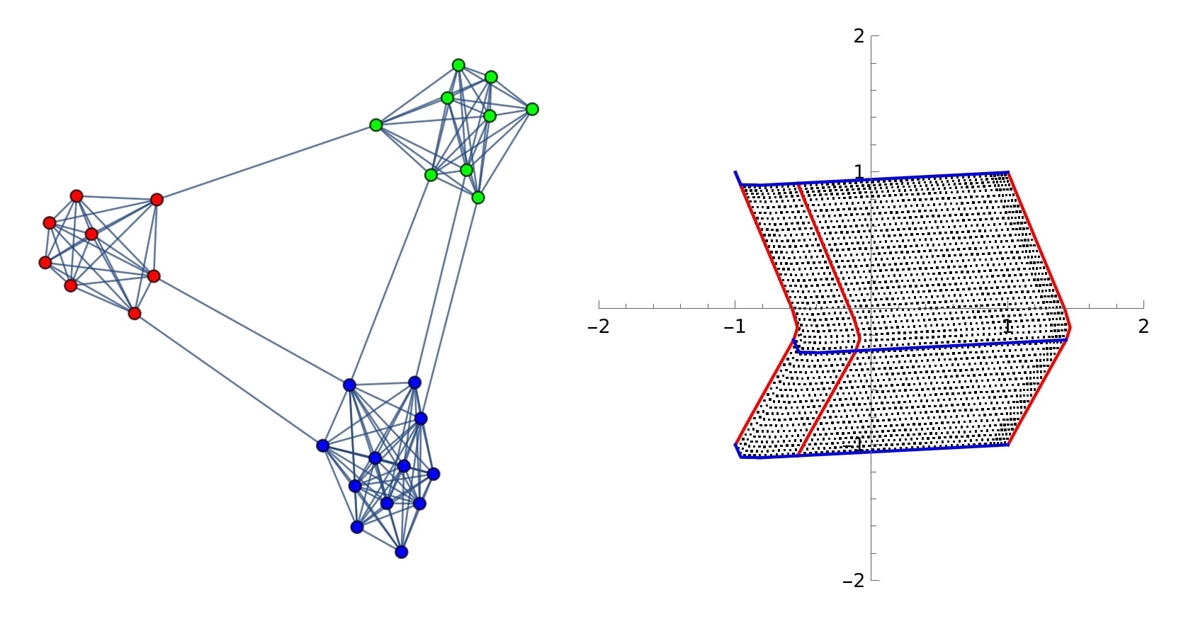
Figure 1: A graph with three well separated clusters, and the image of its Fiedler-carpet.

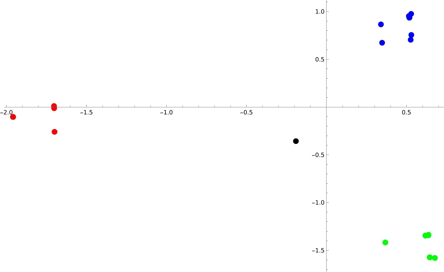
Figure 2: 2-dimensional vertex-representatives of the graph of Figure 1. The black point denotes the approximate root of $f$.

Some remarks are in order:

• Theorem 1 is the generalization of Theorem 2.2.3 of [3]. There, in the $k=2$ case, $2^{k-1}=k$, but in general, the number of clusters is much larger than that of the relevant eigenvectors.

• The statement of the theorem has relevance, since for any $k>0$, the relation $\sum_{j=1}^{k-1}\lambda_{j}<(k-1)\lambda_{k}$ holds; but with analysis of variance considerations, $S_{2^{k-1}}^{2}\leq k-1$ also holds. In particular, when $k=2$, only one eigenvector is used for the representation. The total inertia of the coordinates is 1, and it can be divided into the sum of nonnegative within- and between-cluster inertias. The within-cluster inertia is the sum of the inner variances of the two clusters, which is $S_{2}^{2}$, so it is at most 1. (Here the variances are calculated with respect to the discrete distribution $d_{1},\dots,d_{n}$.) When $(k-1)$-dimensional representatives are used, then the total inertia is $\mathrm{tr}(\bm{X}_{k-1}^{T}\bm{D}\bm{X}_{k-1})=\mathrm{tr}(\bm{I}_{k-1})=k-1$, and the sum of the inner variances is again at most $k-1$, but it is further bounded with $\frac{\sum_{j=1}^{k-1}\lambda_{j}}{\lambda_{k}}$ by Theorem 1.

• The vector $\mathbf{u}_{1}$ is called Fiedler-vector of the (non-normalized) Laplacian. Here we use the first $k-1$ transformed eigenvectors of the normalized Laplacian together, that we call Fiedler-carpet.

4 Applications

We investigated the international migrant stock by the country of origin and destination in the years 2015 and 2019. The focus in on 41 European countries plus the United States of America and Canada. The data is based on the official registered migrants numbers, where columns and rows are corresponding to the country of origin and the country of destination, respectively.

Here the quadratic, but not symmetric edge-weight matrix contains weights of bidirected edges (the diagonal is zero): the $i,j$ entry is the number of persons going $j\to i$. Via SVD of the normalized table, we can find emigration (column) and immigration (row) clusters, between which the migration is the best homogeneous (in terms of discrepancy).

Both for the 2015 and 2019 data, there was a gap after four non-trivial singular values, and therefore the corresponding four singular vector pairs were used to find five emigration and immigration trait clusters.

• Singular values, 2015:

  1, 0.79098, 0.71857, 0.67213, 0.56862, 0.45293, 0.40896, 0.38178, 0.36325, 0.34785, 0.32648, 0.31769, 0.2996, 0.27927, 0.26566, 0.24718, 0.22638, 0.20632, 0.18349, 0.1651, 0.14384, 0.1359, 0.12721, 0.12092, 0.11816, 0.10374, 0.09545, 0.08278, 0.0738, 0.06371, 0.05673, 0.04553, 0.03488, 0.03107, 0.02967, 0.02693, 0.01557, 0.00788, 0.00584, 0.00519, 0.00191, 0.0017, 0.00099.

• Singular values, 2019:

  1, 0.77844, 0.70989, 0.65059, 0.55122, 0.43612, 0.39512, 0.36194, 0.3558, 0.33882, 0.32174, 0.30719, 0.29601, 0.28181, 0.26865, 0.259, 0.22421, 0.1917, 0.17988, 0.1516, 0.13671, 0.13243, 0.12397, 0.11542, 0.10598, 0.09216, 0.08889, 0.07958, 0.06835, 0.06154, 0.05377, 0.04412, 0.03436, 0.03124, 0.02899, 0.02745, 0.01507, 0.00814, 0.00619, 0.0051, 0.00216, 0.00129, 0.00089.

Cluster #	Emigration Countries
1	Austria, Belgium, Bulgaria, Canada, Czechia, Denmark, Finland, France, Germany, Greece, Hungary, Iceland, Ireland, Italy, Latvia, Liechtenstein, Lithuania, Luxembourg, Malta, Monaco, Netherlands, North Macedonia, Norway, Poland, Portugal, Romania, Serbia, Slovakia, Spain, Sweden, Switzerland, United Kingdom, United States of America
2	Bosnia and Herzegovina, Croatia, Montenegro, Slovenia
3	Albania
4	Belarus, Estonia, Republic of Moldova, Ukraine
5	Russian Federation

Table 1: Country memberships of emigration trait clusters, 2015.

Cluster #	Immigration Countries
1	Albania, Austria, Belgium, Bulgaria, Canada, Czechia, Denmark, Finland, France, Germany, Hungary, Iceland, Ireland, Liechtenstein, Luxembourg, Malta, Monaco, Netherlands, Norway, Portugal, Romania, Slovakia, Spain, Sweden, Switzerland, United Kingdom, United States of America
2	Greece, Italy, North Macedonia
3	Bosnia and Herzegovina, Croatia, Montenegro, Serbia, Slovenia
4	Belarus, Estonia, Latvia, Lithuania, Ukraine
5	Poland, Republic of Moldova, Russian Federation

Table 2: Country memberships of immigration trait clusters, 2015.

Cluster #	Emigration Countries
1	Austria, Belgium, Bulgaria, Canada, Czechia, Denmark, Finland, France, Germany, Greece, Hungary, Iceland, Ireland, Italy, Latvia, Liechtenstein, Lithuania, Luxembourg, Malta, Monaco, Netherlands, North Macedonia, Norway, Poland, Portugal, Romania, Serbia, Slovakia, Spain, Sweden, Switzerland, United Kingdom, United States of America
2	Bosnia and Herzegovina, Croatia, Montenegro, Slovenia
3	Albania
4	Belarus, Estonia, Republic of Moldova, Ukraine
5	Russian Federation

Table 3: Country memberships of emigration trait clusters, 2019.

Cluster #	Immigration Countries
1	Albania, Austria, Belgium, Bulgaria, Canada, Czechia, Denmark, Finland, France, Germany, Hungary, Iceland, Ireland, Liechtenstein, Luxembourg, Malta, Monaco, Netherlands, Norway, Portugal, Romania, Slovakia, Spain, Sweden, Switzerland, United Kingdom, United States of America
2	Bosnia and Herzegovina, Croatia, Montenegro, Serbia, Slovenia
3	Greece, Italy, North Macedonia
4	Poland, Republic of Moldova, Russian Federation
5	Belarus, Estonia, Latvia, Lithuania, Ukraine

Table 4: Country memberships of immigration trait clusters, 2019.

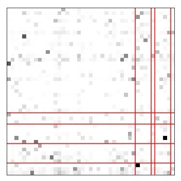
(a) 2015

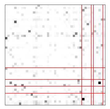
(b) 2019

Figure 3: Immigration–emigration cluster-pairs with the countries rearranged by their cluster memberships. The frequency counts are represented with light to dark squares.

Emigration and immigration trait clusters for 2015 are shown in Table 2 and Table 2, whereas those for 2019, in Table 4 and Table 4. Figures 3 and 3 illustrate the immigration–emigration cluster-pairs with the countries rearranged by their cluster memberships. The frequency counts are represented with light to dark squares.

In 2015, by $\chi^{2}$ test we found the smallest discrepancy between the emigration trait cluster number 2 and immigration trait cluster number 4, i.e. the sub-table formed by them was close to an independent table of rank 1. The clusters were similar in the two years; in 2019, the smallest discrepancy was found between the emigration trait cluster number 2 and immigration trait cluster number 5, i.e. between the Balcanian and Baltic countries in both years.

Correspondence analysis results with cluster memberships are found in Appendix B.

5 Summary

Spectral clustering is for clustering data points or the vertices of a graph based on combinatorial criteria with spectral relaxation. Here we generalize spectral clustering in several ways:

• Instead of simple or edge-weighed graphs consider directed graphs and rectangular arrays of nonnegative entries. For these, the method of correspondence analysis gives low-dimensional representation of the row and column items by means of SVD of the normalized table. This is applied to real-life data.

• Instead of the usual multiway minimum cut objective, we consider discrepancy minimization, for which a near optimal solution is given by the $k$-means algorithm applied to the row and column representatives, where the number of clusters $(k)$ is concluded from the gap in the singular spectrum. There are theoretical results supporting this. Eventually, the near optimal clusters can be refined to decrease discrepancy.

• The number of clusters can be larger than the number of eigenvectors entered in the classification. The two are the same only in case of generalized random or quasirandom graphs, see [8]. In Theorem 1, an exact estimate for the sum of the inner variances of $2^{k-1}$ clusters is given by means of the spectral gap between the $(k-1)$th and $k$th smallest normalized Laplacian eigenvalues by using the Fiedler-carpet of the corresponding eigenvectors.

Appendix A

In the $f:\mathbb{R}\to\mathbb{R}$ case: $f=f_{1}$, $a=a_{1}$ and with the notation $A=\min_{i}x_{1i}$, $B=\max_{i}x_{1i}$ for

$$f(a)=\sum_{i=1}^{n}d_{i}x_{1i}|x_{1i}-a|$$

we have that $f(A)=1$ and $f(B)=-1$. As $f$ is continuous, it must have a root in $(A,B)$, by the Bolzano theorem. Also note that this root of $f$ is around the median of the coordinates of $\mathbf{x}_{1}$ with respect to the discrete measure $d_{1},\dots,d_{n}$.

Then consider the $f=(f_{1},f_{2}):\mathbb{R}^{2}\to\mathbb{R}^{2}$ case. The coordinate functions are stepwise linear, continuous functions. The system of equations is

$$f_{1}(a_{1},a_{2}) =\sum_{i=1}^{n}d_{i}x_{1i}|x_{1i}-a_{1}|+\sum_{i=1}^{n}d_{i}x_{1i}|x_{2i}-a_{2}|=0,$$ (17)

$$f_{2}(a_{1},a_{2}) =\sum_{i=1}^{n}d_{i}x_{2i}|x_{1i}-a_{1}|+\sum_{i=1}^{n}d_{i}x_{2i}|x_{2i}-a_{2}|=0.$$

With the notation $A=\min_{i}x_{1i}$, $B=\max_{i}x_{1i}$, $C=\min_{i}x_{2i}$, $D=\max_{i}x_{2i}$, where $A<0,B>0,C<0,D>0$,

$$f(A,C)=(1,1),\,f(B,D)=(-1,-1),\,f(A,D)=(1,-1),\,f(B,C)=(-1,1).$$

Furthermore, $f(x,y)=(1,1)$ if $x\leq A,\,y\leq C$; $f(x,y)=(-1,-1)$ if $x\geq B,\,y\geq D$; $f(x,y)=(1,-1)$ if $x\leq A,\,y\geq D$; and $f(B,C)=(-1,1)$ if $x\geq B,\,y\leq C$.

We want to show that $f$ has a root within the rectangle $[A,B]\times[C,D]$. By the multivariate version of the Bolzano theorem, the $f$-map of this rectangle is a connected region in $\mathbb{R}^{2}$ that contains the points $(1,1),(-1,-1),(1,-1),(-1,1)$ as ‘corners’. We will show that it contains $(0,0)$ too.

Note that together with $\mathbf{u}_{j}$, the vector $-\mathbf{u}_{j}$ is also a unit-norm eigenvector, so instead of $\mathbf{x}_{j}$ we can as well use $-\mathbf{x}_{j}$ for $j=1,2$, that gives 4 possible domains of $f$: next to the rectangle $[A,B]\times[C,D]$, the rectangles $[-B,-A]\times[C,D]$, $[A,B]\times[-D,-C]$, and $[-B,-A]\times[-D,-C]$ are also closed, bounded regions, and the $f$-images of them show symmetry with respect to the coordinate axes. Therefore, it suffices to prove that the map of the union of them contains the origin. In Section 2, we saw that neither the objective function ($Q_{k}$), nor the clustering is affected by the orientation of the eigenvectors, so the orientation is not denoted in the sequel. Also notice that with counter-orienting $\mathbf{u}_{1}$ or/and $\mathbf{u}_{2}$: if $(a_{1},a_{2})$ is a root of $f$, then $-a_{1}$ instead of $a_{1}$ or/and $-a_{2}$ instead of $a_{2}$ will result in a root of $f$ too.

The images are closed, bounded regions (usually not rectangles), but we will show that the opposite sides of them are parallel curves and sandwich the $f_{1}$ and $f_{2}$ axes, respectively. As the $f$-values sweep the region between these boundaries, the total range should contain the origin. At the end, we take the orientations into consideration to arrive to the expected result.

Now the above, below, right, and left boundaries are investigated.

• Above: Consider the boundary curve between (-1,1) and (1,1). Along that, $a_{2}=C$ and $A<a_{1}<B$. Let $H:=\{i:\,x_{1i}>a_{1}\}$. Then $H\neq\emptyset$ and ${\bar{H}}\neq\emptyset$; further,

  $$f_{2}(a_{1},C) =\sum_{i=1}^{n}d_{i}x_{2i}|x_{1i}-a_{1}|+\sum_{i=1}^{n}d_{i}x_{2i}(x_{2i}-C)=$$ (18)

  $$=\sum_{i\in H}d_{i}x_{2i}(x_{1i}-a_{1})-\sum_{i\in{\bar{H}}}d_{i}x_{2i}(x_{1i}-a_{1})+1$$

  $$=2\sum_{i\in H}d_{i}x_{2i}(x_{1i}-a_{1})+1$$

  $$=2\sum_{i\in{\bar{H}}}d_{i}x_{2i}(a_{1}-x_{1i})+1,$$

  where we intensively used conditions (10).

• Below: Consider the boundary curve between (-1,-1) and (1,-1). Along that, $a_{2}=D$ and $A<a_{1}<B$. Then

  $$f_{2}(a_{1},D) =\sum_{i=1}^{n}d_{i}x_{2i}|x_{1i}-a_{1}|-\sum_{i=1}^{n}d_{i}x_{2i}(x_{2i}-D)=$$ (19)

  $$=\sum_{i\in H}d_{i}x_{2i}(x_{1i}-a_{1})-\sum_{i\in{\bar{H}}}d_{i}x_{2i}(x_{1i}-a_{1})-1=$$

  $$=2\sum_{i\in H}d_{i}x_{2i}(x_{1i}-a_{1})-1$$

  $$=2\sum_{i\in{\bar{H}}}d_{i}x_{2i}(a_{1}-x_{1i})-1.$$

• Between (horizontally): Consider the case when $a_{2}=u\in(C,D)$ fixed and $A<a_{1}<B$. Then

  $$f_{2}(a_{1},u) =\sum_{i=1}^{n}d_{i}x_{2i}|x_{1i}-a_{1}|+\sum_{i=1}^{n}d_{i}x_{2i}|x_{2i}-u|=$$

  $$=\sum_{i\in H}d_{i}x_{2i}(x_{1i}-a_{1})-\sum_{i\in{\bar{H}}}d_{i}x_{2i}(x_{1i}-a_{1})+$$

  $$+\sum_{i:\,x_{2i}>u}d_{i}x_{2i}(x_{2i}-u)+\sum_{i:\,x_{2i}\leq u}d_{i}x_{2i}(u-x_{2i})=$$

  $$=2\sum_{i\in H}d_{i}x_{2i}(x_{1i}-a_{1})-1+2\sum_{i:\,x_{2i}>u}d_{i}x_{2i}^{2}-2u\sum_{i:\,x_{2i}>u}d_{i}x_{2i}.$$

So the $f_{2}(a_{1},u)$ arcs are all parallel to the boundary curves $f_{2}(a_{1},C)$ and $f_{2}(a_{1},D)$ and to each other. In particular,

$$f_{2}(a_{1},0)=2\sum_{i\in H}d_{i}x_{2i}(x_{1i}-a_{1})-1+2\sum_{i:\,x_{2i}>0}d_{i}x_{2i}^{2}.$$

This arc is either closer to the Above or the Below curve (which are in distance 2 from each other), depending on whether $\sum_{i:\,x_{2i}>0}d_{i}x_{2i}^{2}$ is less or greater than $\frac{1}{2}$, but is strictly positive by condition (10). For this reason, if $u$ and $u^{\prime}$ are ‘close’ to 0, then the $f_{2}(a_{1},u)$ and $f_{2}(a_{1},u^{\prime})$ arcs are not identical, otherwise it can happen that for some $u\neq u^{\prime}$:

$$\sum_{i:\,x_{2i}>u}d_{i}x_{2i}^{2}-u\sum_{i:\,x_{2i}>u}d_{i}x_{2i}=\sum_{i:\,x_{2i}>u^{\prime}}d_{i}x_{2i}^{2}-u^{\prime}\sum_{i:\,x_{2i}>u^{\prime}}d_{i}x_{2i}.$$ (20)

The same is true vertically.

• Right: Consider the boundary curve between (1,-1) and (1,1). Along that, $a_{1}=A$ and $C<a_{2}<D$. Let $F:=\{i:\,x_{2i}>a_{2}\}$. Then $F\neq\emptyset$ and ${\bar{F}}\neq\emptyset$; further,

  $$f_{1}(A,a_{2}) =\sum_{i=1}^{n}d_{i}x_{1i}(x_{1i}-A)-\sum_{i=1}^{n}d_{i}x_{1i}|x_{2i}-a_{2}|=$$ (21)

  $$=1+\sum_{i\in F}d_{i}x_{1i}(x_{2i}-a_{2})-\sum_{i\in{\bar{F}}}d_{i}x_{1i}(x_{2i}-a_{2})=$$

  $$=1+2\sum_{i\in F}d_{i}x_{1i}(x_{2i}-a_{2})=$$

  $$=1+2\sum_{i\in{\bar{F}}}d_{i}x_{1i}(a_{2}-x_{2i}).$$

• Left: As from the left, consider the boundary curve between (-1,-1) and (-1,1). Along that, $a_{1}=B$ and $C<a_{2}<D$. Then

  $$f_{1}(B,a_{2}) =-1+2\sum_{i\in F}d_{i}x_{1i}(x_{2i}-a_{2})=$$ (22)

  $$=-1+2\sum_{i\in{\bar{F}}}d_{i}x_{1i}(a_{2}-x_{2i}).$$

• Between (vertically): Consider the case when $a_{1}=v\in(A,B)$ fixed and $C<a_{2}<D$. Then

  $$f_{1}(v,a_{2})=1+2\sum_{i\in F}d_{i}x_{1i}(x_{2i}-a_{2})-1+2\sum_{i:\,x_{1i}>v}d_{i}x_{1i}^{2}-2v\sum_{i:\,x_{1i}>v}d_{i}x_{1i}.$$

So the $f_{1}(v,a_{2})$ arcs are all parallel to the boundary curves $f_{1}(A,a_{2})$ and $f_{1}(B,a_{2})$ and to each other. In particular,

$$f_{1}(0,a_{2})=2\sum_{i\in F}d_{i}x_{1i}(x_{2i}-a_{2})-1+2\sum_{i:\,x_{1i}>0}d_{i}x_{1i}^{2}.$$

This arc is either closer to the Right or the Left curve (which are in distance 2 from each other), depending on whether $\sum_{i:\,x_{1i}>0}d_{i}x_{1i}^{2}$ is less or greater than $\frac{1}{2}$, but is strictly positive by condition (10). For this reason, if $v$ and $v^{\prime}$ are ‘close’ to 0, then the $f_{1}(v,a_{2})$ and $f_{1}(v^{\prime},a_{2})$ arcs are not identical, otherwise it can happen that for some $v\neq v^{\prime}$:

$$\sum_{i:\,x_{1i}>v}d_{i}x_{1i}^{2}-v\sum_{i:\,x_{1i}>v}d_{i}x_{1i}=\sum_{i:\,x_{`i}>v^{\prime}}d_{i}x_{1i}^{2}-v^{\prime}\sum_{i:\,x_{1i}>v^{\prime}}d_{i}x_{1i}.$$ (23)

Therefore, any grid on the rectangle of the domain (its horizontal and vertical lines parallel to the $a_{1}$ and $a_{2}$ axes) is mapped by $f$ onto a lattice with horizontal and vertical, parallel arcs. This proves that $f$ is one-to-one whenever these arcs are not identical. The possible inconvenient phenomenon, when both Equations (20) and (23) hold for some $u\neq u^{\prime}$ and $v\neq v^{\prime}$ pairs, is experienced at the dark parts of Figure 5 near the boundaries. However, $f$ is injective in the neighborhood of the origin that does not contain any eigenvector coordinates (because there it has purely linear coordinate functions). This also depends on the underlying graph: if it shows symmetries, then its weighted Laplacian has multiple eigenvalues and/or multiple coordinates of the eigenvectors that may cause complications.

To prove that the Above–Below boundaries sandwich the $f_{1}$ axis and the Right–Left boundaries sandwich the $f_{2}$ axis, respectively, the following investigations are made. Because the investigations are of similar vein, only the first of them will be discussed in details. We distinguish between eight cases (denoted by an acronym), depending on, which half of which boundary is considered. The estimates are supported by specific orientations of the unit norm eigenvectors. If $\mathbf{u}_{1}$ is oriented so that for the coordinates of of $\mathbf{x}_{1}=\bm{D}^{-1/2}\mathbf{u}_{1}$

$$\sum_{i:\,x_{1i}>0}d_{i}x_{1i}^{2}<\frac{1}{2}$$

holds, then it is called positive orientation, whereas, the opposite is negative. Likewise, he orientation of $\mathbf{u}_{2}$ is positive if for the coordinates of of $\mathbf{x}_{2}=\bm{D}^{-1/2}\mathbf{u}_{2}$

$$\sum_{i:\,x_{2i}>0}d_{i}x_{2i}^{2}<\frac{1}{2}$$ (24)

holds, otherwise it is negative.

• (Above boundary, Left half), when $a_{1}>0$: using the last but one line of Equation (18),

  $$f_{2}(a_{1},C) =2\sum_{i\in H}d_{i}x_{2i}(x_{1i}-a_{1})+1$$

  $$=2\sum_{i\in H,\,x_{2i}>0}d_{i}x_{2i}(x_{1i}-a_{1})+2\sum_{i\in H,\,x_{2i}\leq 0}d_{i}x_{2i}(x_{1i}-a_{1})+1$$

  $$\geq 2\sum_{i\in H,\,x_{2i}\leq 0}d_{i}x_{2i}(x_{1i}-a_{1})+1.$$

  To prove that $f_{2}(a_{1},C)\geq 0$ it suffices to prove that

  $$\sum_{i\in H,\,x_{2i}\leq 0}d_{i}x_{2i}(x_{1i}-a_{1})\geq-\frac{1}{2},$$

  which is equivalent to

  $$\sum_{i\in H,\,x_{2i}\leq 0}d_{i}(-x_{2i})(x_{1i}-a_{1})\leq\frac{1}{2}.$$

  We use the Cauchy–Schwarz inequality by keeping in mind that $x_{1i}-a_{1}>0$ $(i\in H)$ and because of $a_{1}>0$, $x_{1i}-a_{1}<x_{1i}$. Therefore,

  $$[\sum_{i\in H\,x_{2i}\leq 0}(\sqrt{d_{i}}(-x_{2i}))(\sqrt{d_{i}}(x_{1i}-a_{1}))]^{2}\leq[\sum_{i\in H\,x_{2i}\leq 0}d_{i}x_{2i}^{2}][\sum_{i\in H\,x_{2i}\leq 0}d_{i}x_{1i}^{2}]\leq\frac{1}{2}\frac{1}{2}$$

  holds true if $\mathbf{u}_{1}$ is positively and $\mathbf{u}_{2}$ is negatively oriented.

• (Above boundary, Right half), when $a_{1}\leq 0$: using the last line of Equation (18), to prove that $f_{2}(a_{1},C)\geq 0$ it suffices to prove that

  $$\sum_{i\in{\bar{H}},\,x_{2i}\leq 0}d_{i}x_{2i}(a_{1}-x_{1i})\geq-\frac{1}{2},$$

  which is equivalent to

  $$\sum_{i\in{\bar{H}},\,x_{2i}\leq 0}d_{i}(-x_{2i})(a_{1}-x_{1i})\leq\frac{1}{2}.$$

  We again use the Cauchy–Schwarz inequality by keeping in mind that $a_{1}-x_{1i}\geq 0$ $(i\in{\bar{H}})$ and $a_{1}-x_{1i}=-x_{i1}-(-a_{1})\leq-x_{1i}$ as now $-a_{1}\geq 0$ and $-x_{1i}>-a_{1}$. Therefore,

  $$[\sum_{i\in{\bar{H}},x_{2i}\leq 0}(\sqrt{d_{i}}(-x_{2i}))(\sqrt{d_{i}}(a_{1}-x_{1i}))]^{2}\leq[\sum_{i\in{\bar{H}},x_{2i}\leq 0}d_{i}x_{2i}^{2}][\sum_{i\in{\bar{H}},x_{2i}\leq 0}d_{i}(-x_{1i})^{2}]\leq\frac{1}{2}\frac{1}{2}$$

  holds true with negatively orienting $\mathbf{u}_{1}$ and negatively $\mathbf{u}_{2}$.

• (Below boundary, Left half), when $a_{1}>0$: using the last but one line of Equation (19),

  $$f_{2}(a_{1},D) =2\sum_{i\in H}d_{i}x_{2i}(x_{1i}-a_{1})-1$$

  $$=2\sum_{i\in H,\,x_{2i}<0}d_{i}x_{2i}(x_{1i}-a_{1})+2\sum_{i\in H,\,x_{2i}\geq 0}d_{i}x_{2i}(x_{1i}-a_{1})-1$$

  $$\leq 2\sum_{i\in H,\,x_{2i}\geq 0}d_{i}x_{2i}(x_{1i}-a_{1})-1.$$

  To prove that $f_{2}(a_{1},D)\leq 0$ it suffices to prove that

  $$\sum_{i\in H,\,x_{2i}\geq 0}d_{i}x_{2i}(x_{1i}-a_{1})\leq\frac{1}{2}.$$

  We use the Cauchy–Schwarz inequality by keeping in mind that $x_{1i}-a_{1}>0$ $(i\in H)$ and because of $a_{1}>0$, $x_{1i}-a_{1}<x_{1i}$. Therefore,

  $$[\sum_{i\in H\,x_{2i}\geq 0}(\sqrt{d_{i}}x_{2i})(\sqrt{d_{i}}(x_{1i}-a_{1}))]^{2}\leq[\sum_{i\in H\,x_{2i}\geq 0}d_{i}x_{2i}^{2}][\sum_{i\in H\,x_{2i}\geq 0}d_{i}x_{1i}^{2}]\leq\frac{1}{2}\frac{1}{2}$$

  holds true if $\mathbf{u}_{1}$ is positively and $\mathbf{u}_{2}$ is positively oriented.

• (Below boundary, Right half), when $a_{1}\leq 0$: using the last line of Equation (19), to prove that $f_{2}(a_{1},D)\leq 0$ it suffices to prove that

  $$\sum_{i\in{\bar{H}},\,x_{2i}\geq 0}d_{i}x_{2i}(a_{1}-x_{1i})\leq\frac{1}{2}.$$

  We again use the Cauchy–Schwarz inequality by keeping in mind that $a_{1}-x_{1i}\geq 0$ $(i\in{\bar{H}})$ and $a_{1}-x_{1i}=-x_{i1}-(-a_{1})\leq-x_{1i}$ as now $-a_{1}\geq 0$ and $-x_{1i}>-a_{1}$. Therefore,

  $$[\sum_{i\in{\bar{H}},x_{2i}\geq 0}(\sqrt{d_{i}}x_{2i})(\sqrt{d_{i}}(a_{1}-x_{1i}))]^{2}\leq[\sum_{i\in{\bar{H}},x_{2i}\geq 0}d_{i}x_{2i}^{2}][\sum_{i\in{\bar{H}},x_{2i}\geq 0}d_{i}(-x_{1i})^{2}]\leq\frac{1}{2}\frac{1}{2}$$

  holds true with negatively orienting $\mathbf{u}_{1}$ and positively $\mathbf{u}_{2}$.

• (Right boundary, Below half), when $a_{2}>0$: using the last but one line of Equation (21),

  $$f_{1}(A,a_{2})\geq 2\sum_{i\in F,\,x_{1i}\leq 0}d_{i}x_{1i}(x_{2i}-a_{2})+1.$$

  To prove that $f_{1}(A,a_{2})\geq 0$ it suffices to prove that

  $$\sum_{i\in F,\,x_{1i}\leq 0}d_{i}x_{1i}(x_{2i}-a_{2})\geq-\frac{1}{2},$$

  which is equivalent to

  $$\sum_{i\in F,\,x_{1i}\leq 0}d_{i}(-x_{1i})(x_{2i}-a_{2})\leq\frac{1}{2}.$$

  By the Cauchy–Schwarz inequality,

  $$[\sum_{i\in F\,x_{1i}\leq 0}(\sqrt{d_{i}}(-x_{1i}))(\sqrt{d_{i}}(x_{2i}-a_{2}))]^{2}\leq[\sum_{i\in F\,x_{1i}\leq 0}d_{i}x_{1i}^{2}][\sum_{i\in F\,x_{1i}\leq 0}d_{i}x_{2i}^{2}]\leq\frac{1}{2}\frac{1}{2}$$

  holds true if $\mathbf{u}_{1}$ is negatively and $\mathbf{u}_{2}$ is positively oriented.

• (Right boundary, Above half), when $a_{2}\leq 0$: using the last line of Equation (21), to prove that $f_{1}(A,a_{2})\geq 0$ it suffices to prove that

  $$\sum_{i\in{\bar{F}},\,x_{1i}\leq 0}d_{i}x_{1i}(a_{2}-x_{2i})\geq-\frac{1}{2},$$

  which is equivalent to

  $$\sum_{i\in{\bar{F}},\,x_{1i}\leq 0}d_{i}(-x_{1i})(a_{2}-x_{2i})\leq\frac{1}{2}.$$

  By the Cauchy–Schwarz inequality,

  $$[\sum_{i\in{\bar{F}},x_{1i}\leq 0}(\sqrt{d_{i}}(-x_{1i}))(\sqrt{d_{i}}(a_{2}-x_{2i}))]^{2}\leq[\sum_{i\in{\bar{F}},x_{1i}\leq 0}d_{i}x_{1i}^{2}][\sum_{i\in{\bar{F}},x_{1i}\leq 0}d_{i}(-x_{2i})^{2}]\leq\frac{1}{2}\frac{1}{2}$$

  holds true with negatively orienting $\mathbf{u}_{1}$ and negatively $\mathbf{u}_{2}$.

• (Left boundary, Below half), when $a_{2}>0$: using the last but one line of Equation (22),

  $$f_{1}(B,a_{2})=2\sum_{i\in F}d_{i}x_{1i}(x_{2i}-a_{2})-1\leq 2\sum_{i\in F,\,x_{1i}\geq 0}d_{i}x_{1i}(x_{2i}-a_{2})-1.$$

  To prove that $f_{1}(B,a_{2})\leq 0$ it suffices to prove that

  $$\sum_{i\in F,\,x_{1i}\geq 0}d_{i}x_{1i}(x_{2i}-a_{2})\leq\frac{1}{2},$$

  By the Cauchy–Schwarz inequality,

  $$[\sum_{i\in F\,x_{1i}\geq 0}(\sqrt{d_{i}}x_{1i})(\sqrt{d_{i}}(x_{2i}-a_{2}))]^{2}\leq[\sum_{i\in F\,x_{1i}\geq 0}d_{i}x_{1i}^{2}][\sum_{i\in F\,x_{1i}\geq 0}d_{i}x_{2i}^{2}]\leq\frac{1}{2}\frac{1}{2}$$

  holds true if $\mathbf{u}_{1}$ is positively and $\mathbf{u}_{2}$ is positively oriented.

• (Left boundary, Above half), when $a_{2}\leq 0$: using the last line of Equation (22), to prove that $f_{1}(B,a_{2})\leq 0$ it suffices to prove that

  $$\sum_{i\in{\bar{F}},\,x_{1i}\geq 0}d_{i}x_{1i}(a_{2}-x_{2i})\leq\frac{1}{2}.$$

  By the Cauchy–Schwarz inequality,

  $$[\sum_{i\in{\bar{F}},x_{1i}\geq 0}(\sqrt{d_{i}}x_{1i})(\sqrt{d_{i}}(a_{2}-x_{2i}))]^{2}\leq[\sum_{i\in{\bar{F}},x_{1i}\geq 0}d_{i}x_{1i}^{2}][\sum_{i\in{\bar{F}},x_{1i}\geq 0}d_{i}(-x_{2i})^{2}]\leq\frac{1}{2}\frac{1}{2}$$

  holds true with positively orienting $\mathbf{u}_{1}$ and negatively $\mathbf{u}_{2}$.

So the convenient orientation of the AL scenario matches that of the LA one. Similarly, the AR-RA, BL-LB, and BR-RB scenatios can be ralized with the same orientation of $\mathbf{u}_{1},\mathbf{u}_{2}$. Namely, the first quadrant of the domain $(a_{1}\geq 0,a_{2}\geq 0)$ is mapped to the third quadrant of the range, in which part the $(+,+)$ orientation; the second quadrant of the domain $(a_{1}\leq 0,a_{2}\geq 0)$ is mapped to the fourth quadrant of the range, in which part the $(-,+)$ orientation; the third quadrant of the domain $(a_{1}\leq 0,a_{2}\leq 0)$ is mapped to the first quadrant of the range, in which part the $(-,-)$ orientation; the fourth quadrant of the domain $(a_{1}\geq 0,a_{2}\leq 0)$ is mapped to the second quadrant of the range, in which part the $(+,-)$ orientation of $(\mathbf{x}_{1},\mathbf{x}_{2})$ works.

Therefore, the ranges corresponding to the four quadrants intesect, and so, the ranges under the four different orientations are connected regions (by the multivariate analogue of the Bolzano theorem) and all contain the ‘corners’ $(1,1),(-1,-1),(1,-1),(-1,1)$. Therefore, the union is also a connected region in $\mathbb{R}^{2}$. As it is bounded from above, from below, from the right, and from the left with curves that enclose the origin, it should contain the origin too. Moreover, there should be an orientation and a quadrant that contains the origin. It is not important, but note that with any orientation, a quadrant contains the origin, which is the map of the root we are looking for.

Alternatively, notice that in the AL case, $f_{2}(a_{1},C)$ is greater than or less than 1, depending on whether the absolute value of $\sum_{i\in H,\,x_{2i}>0}d_{i}x_{2i}(x_{1i}-a_{1})$ or that of $\sum_{i\in H,\,x_{2i}\leq 0}d_{i}x_{2i}(x_{1i}-a_{1})$ is larger. By the Cauchy–Schwarz inequality this happens with the positive orientation of $\mathbf{u}_{1}$ and either with the positive or negative orientation of $\mathbf{u}_{2}$. Simultaneously, in the BL case, $f_{2}(a_{1},D)$ greater than or less than -1, depending on whether the absolute value of $\sum_{i\in H,\,x_{2i}>0}d_{i}x_{2i}(x_{1i}-a_{1})$ or that of $\sum_{i\in H,\,x_{2i}\leq 0}d_{i}x_{2i}(x_{1i}-a_{1})$ is larger. So with the positive orientation of $\mathbf{u}_{1}$ and either with the positive or negative orientation of $\mathbf{u}_{2}$, $f_{2}(a_{1},C)$ and $f_{2}(a_{1},D)$ are between -2 and 2, they are parallel, in distance 2 from each other and sandwich the $f_{1}$ axis.

Likewise, the AR,BR estimates imply that with the negative orientation of $\mathbf{u}_{1}$ and either with the positive or negative orientation of $\mathbf{u}_{2}$, $f_{2}(a_{1},C)$ and $f_{2}(a_{1},D)$ are between -2 and 2, they are parallel, in distance 2 from each other and sandwich the $f_{1}$ axis. However, changing the orientation of $\mathbf{u}_{1}$ just means that $-a_{1}$ instead of $a_{1}$ can be in the root of $f$.

Vertically, the RB,LB estimates imply that with the positive orientation of $\mathbf{u}_{2}$ and either with the positive or negative orientation of $\mathbf{u}_{1}$, $f_{2}(A,a_{2})$ and $f_{2}(B,a_{2})$ are between -2 and 2, they are parallel, in distance 2 from each other and sandwich the $f_{2}$ axis. Likewise, the AR,LA estimates imply that with the negative orientation of $\mathbf{u}_{2}$ and either with the positive or negative orientation of $\mathbf{u}_{1}$, $f_{2}(A,a_{2})$ and $f_{2}(B,a_{2})$ are between -2 and 2, they are parallel, in distance 2 from each other and sandwich the $f_{2}$ axis. However, changing the orientation of $\mathbf{u}_{2}$ just means that $-a_{2}$ instead of $a_{2}$ can be in the root of $f$.

As two of these orientations match each other, the $f_{1}$ and $f_{2}$ axes are sandwiched, and so, the origin should be included.

In Figure 5 we show the images of four different possible orientations of the Fiedler-carpet associated with the graph in Figure 4. The $(+,+)$ orientation is shown in the top right, the $(-,-)$ in the bottom left, the $(+,-)$ in the bottom right, and the $(-,+)$ in the top left. Notice that the ranges with the $(+,+)$ and the $(-,-)$ orientation are the same; the $(+,-)$ and $(-,+)$ orientations are reflections of each other across the vertical axis; the $(+,-)$ and $(+,+)$ orientations are reflections of each other across the horizontal axis; consequently the $(-,+)$ and $(+,+)$ orientations are reflections of each other across the origin.

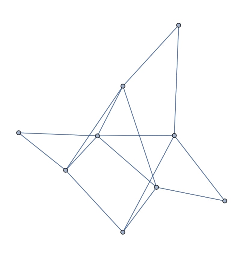
Figure 4: Graph with graph6 string HFRJIOY.

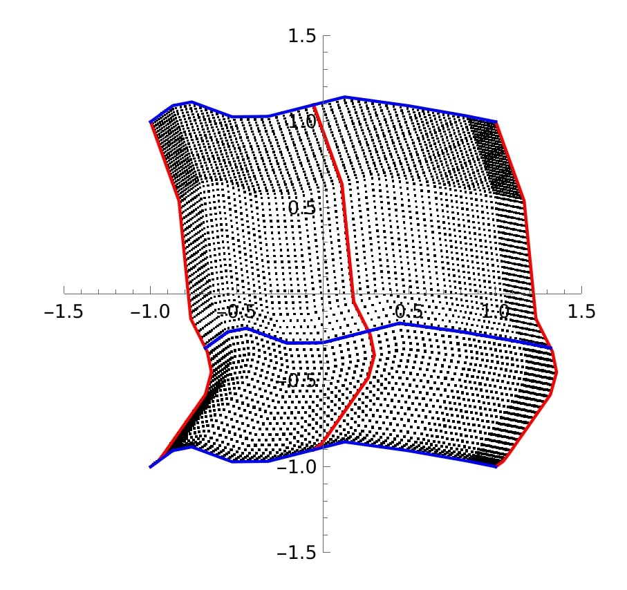
(a) $(-,+)$

(b) $(-,-)$

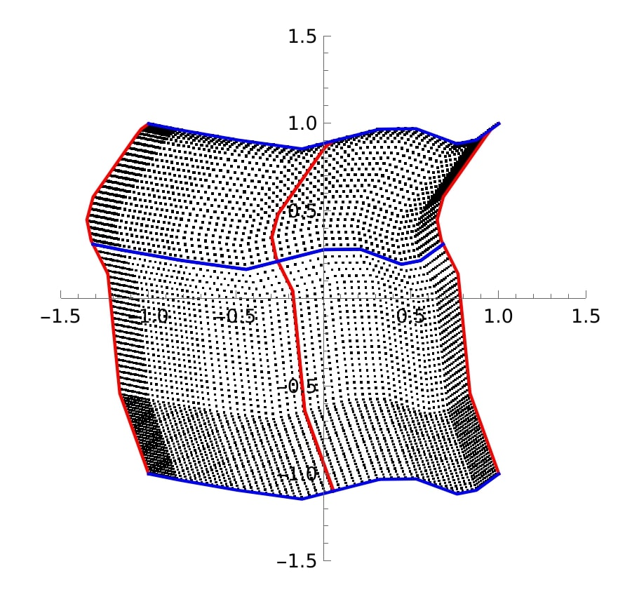
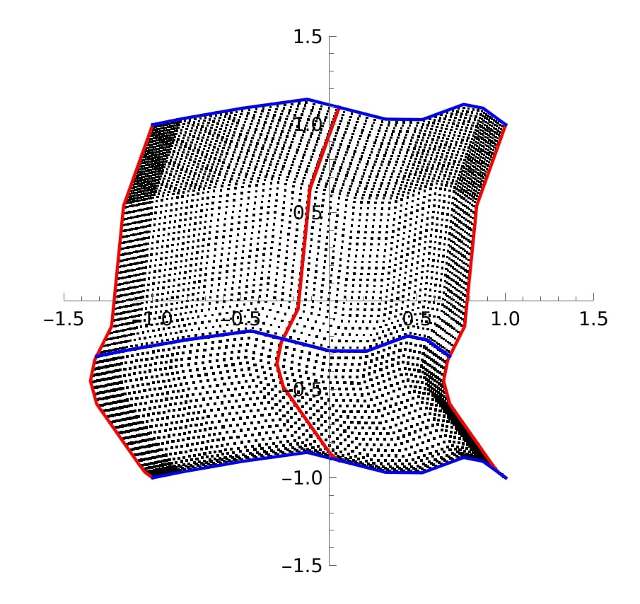
(c) $(+,+)$

(d) $(+,-)$

Figure 5: Images of the four possible orientations of the 2-dimensional Fiedler-carpet of the graph in Figure 4.

We can also plot the map of the three-dimensional Fiedler-carpet of this graph. In Figure 6 different viewpoints are shown. The blue, orange, and green lines are the coordinate axes in $\mathbb{R}^{3}$. As can be seen from the images, they intersect at the origin inside of the three-dimensional body. Every plot we have created shows this intersection lying inside the map of the three-dimensional Fiedler-carpet.

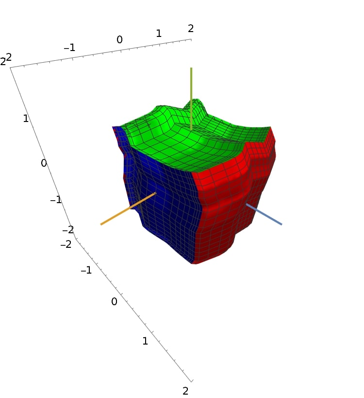
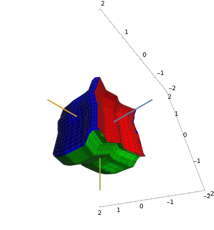
Figure 6: Image of the 3-dimensional Fiedler-carpet, in two different viewpoints, of the graph in Figure 4.

If $k>2$, then $f:\mathbb{R}^{k}\to\mathbb{R}^{k}$ maps the $k$-dimensional hyper-rectangle with vertices of $j$th coordinate $\min_{i}x_{ji}$ or $\max_{i}x_{ji}$ into the $k$-dimensional region with vertices of $j$th coordinate $\pm 1$.

Along the 1-dimensional faces of this $k$-dimensional range, all but one $a_{i}$ is fixed at its minimum/maximum. Without loss of generality, assume that $A<a_{1}<B$. Akin to the $k=2$ case, we are able to show that for each $A<a_{1}<B$: $f_{j}(a_{1},M_{-1})\geq 0$ and $f_{j}(a_{1},{\tilde{M}}_{-1})\leq 0$ $(j=2,\dots,k)$, where $M_{-1}=(\min_{m}x_{2m},\dots,\min_{m}x_{km})$ is the $(k-1)$-tuple of the values of $a_{2},\dots,a_{k}$ all fixed at their minimum and ${\tilde{M}}_{-1}=(\max_{m}x_{2m},\dots,\max_{m}x_{km})$ is the $(k-1)$-tuple of the values of $a_{2},\dots,a_{k}$ all fixed at their maximum values, respectively.

Indeed, for $j=2,\dots,k$:

$$f_{j}(a_{1},M_{-1}) =\sum_{i=1}^{n}d_{i}x_{ji}|x_{1i}-a_{1}|+\sum_{l=2}^{k}\sum_{i=1}^{n}d_{i}x_{ji}(x_{li}-\min_{m}x_{lm})=$$

$$=\sum_{i=1}^{n}d_{i}x_{ji}|x_{1i}-a_{1}|+1+0=$$

$$=2\sum_{i\in H}d_{i}x_{ji}(x_{1i}-a_{1})+1=$$

$$=2\sum_{i\in{\bar{H}}}d_{i}x_{ji}(a_{1}-x_{1i})+1$$

as in the second double summation, only the term for $l=j$ is 1, the others are zeros.

Likewise,

$$f_{j}(a_{1},{\tilde{M}}_{-1}) =\sum_{i=1}^{n}d_{i}x_{ji}|x_{1i}-a_{1}|+\sum_{l=2}^{k}\sum_{i=1}^{n}d_{i}x_{ji}(x_{li}-\max_{m}x_{lm})=$$

$$=\sum_{i=1}^{n}d_{i}x_{ji}|x_{1i}-a_{1}|-1+0=$$

$$=2\sum_{i\in H}d_{i}x_{ji}(x_{1i}-a_{1})-1=$$

$$=2\sum_{i\in{\bar{H}}}d_{i}x_{ji}(a_{1}-x_{1i})-1.$$

as in the second double summation, only the term for $l=j$ is -1, the others are zeros. Note that counter-orienting $\mathbf{u}_{1}$ just results in $-a_{1}$ instead of $a_{1}$ in the root of $f$.

The corresponding ‘corners’ are: $f(A,M_{-1})=(1,1,\dots,1)$, $f(B,M_{-1})=(-1,1,\dots,1)$, $f(A,{\tilde{M}}_{-1})=(1,-1,\dots,-1)$, and $f(B,{\tilde{M}}_{-1})=(-1,-1,\dots,-1)$. These points are in one hyperplane, in which the pieces of the parallel arcs $f_{j}(a_{1},M_{-1})$ and $f_{j}(a_{1},{\tilde{M}}_{-1})$ sandwich the $f_{1}$ axis $(j=2,\dots,k)$. The same is true when another $a_{j}$ moves along a 1-dimensional face and the others are fixed at their minima/maxima. Therefore, the connected regions between these parallel curves sandwich the corresponding coordinate axes, respectively. Consequently, their intersection, which is subset of the whole connected region, contains the origin too.

Appendix B

Pairwise plots of the correspondence analysis results based on the first three coordinate axes (coordinates of the left singular vectors for imigration and right singular vectors for emigration data) are shown in Figures 7 and 7 for the two years. The cluster memberships obtained in Section 4 are illustrated with different colors.

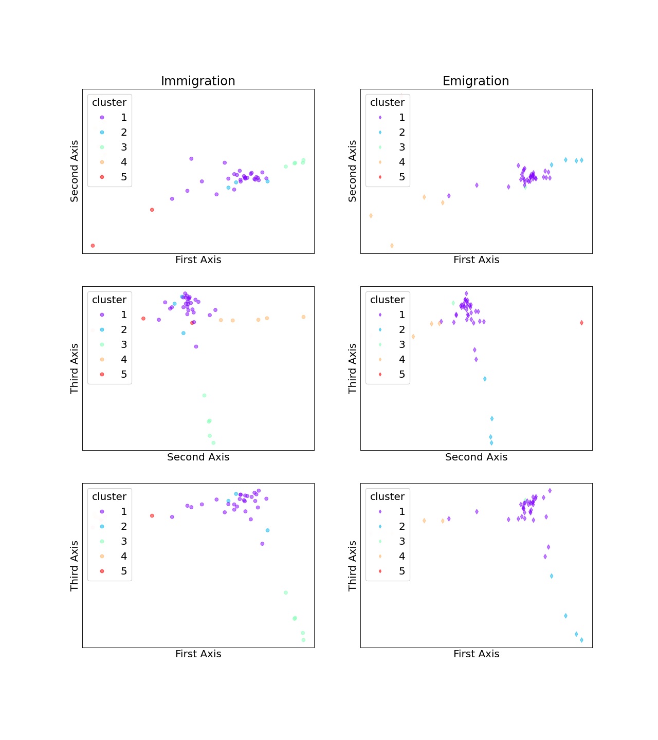
(a) 2015

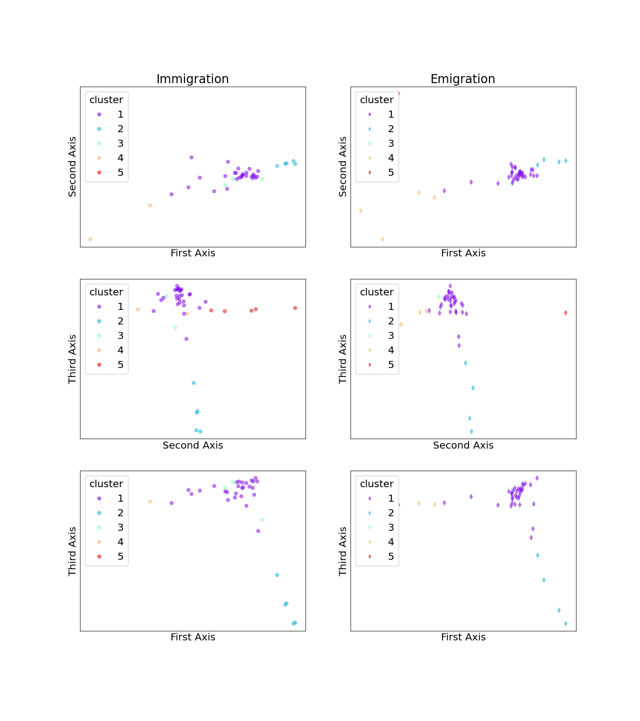
(b) 2019

Figure 7: Pairwise plots of the correspondence analysis results based on the first three singular vector pairs, enhanced with the cluster memberships, illustrated by different colors.

References

- [1] Alon, N., Coja-Oghlan, A., Han, H., Kang, M., Rödl, V., and Schacht, M., Quasi-randomness and algorithmic regularity for graphs with general degree distributions. Siam J. Comput. 39 (6) (2010), 2336–2362.
- [2] Alpert, C.J. and Yao, S.-Z., Spectral partitioning: the more eigenvectors, the better. In Proc. 32nd ACM/IEEE International Conference on Design Automation (Preas BT, Karger PG, Nobandegani BS and Pedram M eds) (1995), pp. 195–200. Association of Computer Machinery, New York.
- [3] Bolla, M. and Tusnády, G., Spectra and Optimal Partitions of Weighted Graphs. Discret. Math. 128 (1994), 1–20.
- [4] Bolla, M., Friedl, K. and Krámli, A., Singular value decomposition of large random matrices (for two-way classification of microarrays). J. Multivariate Anal. 101 (2010), 434–446.
- [5] Bolla, M., Penalized versions of the Newman–Girvan modularity and their relation to multi-way cuts and k-means clustering. Phys. Rev. E 84 (2011), 016108.
- [6] Bolla, M., Spectral Clustering and Biclusterig, Wiley, 2013.
- [7] Bolla, M., Relating multiway discrepancy and singular values of nonnegative rectangular matrices, Discrete Applied Mathematics 203 (2016), 26-34.
- [8] Bolla, M., Generalized quasirandom properties of expanding graph sequences, Nonlinearity 33 No.4 (2020), 1405-1424.
- [9] Bollobás, B. and Nikiforov, V., Hermitian matrices and graphs: singular values and discrepancy. Discrete Mathematics 285 (2004), 17–32.
- [10] Chung, F., Spectral Graph Theory, CBMS Regional Conference Series in Mathematics 92 (1997). American Mathematical Society, Providence RI.
- [11] Chung, F., Graham, R., Quasi-random graphs with given degree sequences, Random Struct. Algorithms 12 (2008), 1–19.
- [12] Cvetković, D. M., Doob, M. and Sachs, H., Spectra of Graphs. Academic Press, New York, 1979.
- [13] Faust, K., Using correspondence analysis for joint displays of affiliation networks. In Models and Methods in Social Network Analysis Vol. 7 (2005), (Carrington PJ and Scott J eds), pp. 117–147. Cambridge Univ. Press, Cambridge.
- [14] Fiedler, M., Algebraic connectivity of graphs. Czech. Math. J. 23 (1973), 298–305.
- [15] Hoffman, A. J., Eigenvalues and partitionings of the edges of a graph. Linear Algebra Appl. 5 (1972), 137–146.
- [16] Hoory, S., Linial, N/ and Widgerson, A., Expander graphs and their applications. Bull. Amer. Math. Soc. (N. S.) 43 (2006), 439–561.
- [17] Kluger, Y., Basri, R., Chang, J. T. and Gerstein, M., Spectral biclustering of microarray data: coclustering genes and conditions. Genome Res. 13 (2003), 703–716.
- [18] Von Luxburg, U., A tutorial on spectral clustering, Stat. Comput. 17 (2006), 395–416.
- [19] Mohar, B., Isoperimetric inequalities, growth and the spectrum of graphs. Linear Algebra Appl. 103 (1988), 119–131.
- [20] Newman, M. E. J., Networks, An Introduction. Oxford University Press, 2010.
- [21] Ng, A. Y., Jordan, M. I. and Weiss, Y., On spectral clustering: analysis and an algorithm. In Proc. 14th Neural Information Processing Systems Conference (NIPS 2001) (Dietterich TG, Becker S and Ghahramani Z eds), pp. 849–856 (2001). MIT Press, Cambridge, USA.
- [22] Ostrovsky et al., The effectiveness of Lloyd-type methods for the -means problem, J. ACM 59 (6), Article 28 (2012).
- [23] Shi, J. and Malik, J., Normalized cuts and image segmentation. IEEE Trans. Pattern Anal. Mach. Intell. 22 (2000), 888–905.
- [24] Szemerédi, E., Regular partitions of graphs. In Colloque Inter. CNRS. No. 260, Problémes Combinatoires et Théorie Graphes (Bermond J-C, Fournier J-C, Las Vergnas M and Sotteau D eds), pp. 399–401 (1976).