CERN-TH-2021-218 Nonperturbative running of the quark mass for $N_{f}=3$ QCD from the chirally rotated Schrödinger Functional

Abstract

We study the Renormalisation Group (RG) running of the quark mass, for $N_{\mathrm{\scriptstyle f}}=3$ QCD with Wilson fermions in a mixed action setup, with standard Schrödinger Functional (SF) boundary conditions for sea quarks and chirally rotated Schrödinger Functional ($\chi$SF) boundary conditions for valence quarks. This necessitates the tuning of the boundary factor $z_{\rm f}(g_{0}^{2})$ of the $\chi$SF valence action, in order to ensure that QCD symmetries are fully recovered in the continuum. The properties of this novel setup are monitored through the ratios $Z_{\rm\scriptscriptstyle S}/Z_{\rm\scriptscriptstyle P}$ and $\Sigma_{\rm\scriptscriptstyle S}/\Sigma_{\rm\scriptscriptstyle P}$ of the renormalisation parameters and step scaling functions of the scalar and pseudoscalar densities. Where comparison is possible, our $Z_{\rm\scriptscriptstyle S}/Z_{\rm\scriptscriptstyle P}$ results are found to agree with previous determinations, based on a mass ratio method de Divitiis et al. (2019) and Ward identities Heitger et al. (2020, 2021), with Schrödinger Functional boundary conditions. The behaviour of $\Sigma_{\rm\scriptscriptstyle S}/\Sigma_{\rm\scriptscriptstyle P}$ confirms the theoretical expectations of $\chi$SF QCD, related to the restoration of the theory’s symmetries in the continuum limit. From the step scaling function of the pseudoscalar density we obtain the quark mass RG-running function from hadronic to perturbative energy scales. This is fully compatible with the earlier result obtained in a similar setup for Wilson quarks with Schrödinger Functional boundary conditions Campos et al. (2018), and provides a strong universality test for the two lattice setups.

I Introduction

The chirally rotated Schrödinger functional ($\chi$SF) Sint (2011) is a variant of the Schrödinger functional (SF) renormalisation scheme, which enables us to obtain renormalisation parameters and lattice step scaling functions, which are “automatically” $O(a)$-improved.

At the formal level, continuum massless QCD with SF boundary conditions (SF-QCD) is equivalent to the one with $\chi$SF boundaries ($\chi$SF-QCD), as one is obtained from the other by suitable redefinitions of the fermion fields, which are non-anomalous chiral rotations in isospin space. These redefinitions also modify the form of the various symmetries of the theory in the $\chi$SF setup. In particular, standard parity ${\cal P}$ in SF-QCD is chirally rotated to the so-called ${\cal P}_{5}$ symmetry in $\chi$SF-QCD. When massless QCD is regularised with Wilson fermions, the strict equivalence between the theories with SF and $\chi$SF boundaries is lost. A consequence of this is that lattice QCD with SF boundaries (SF-LQCD) retains ${\cal P}$-symmetry, while its $\chi$SF counterpart ($\chi$SF-LQCD) is not ${\cal P}_{5}$ symmetric. The restoration of ${\cal P}_{5}$ in the continuum limit requires the introduction of a new counterterm at the time boundaries with a coefficient $z_{\rm f}(g_{0}^{2})$. The new counterterm must be tuned by imposing that a ${\cal P}_{5}$-odd correlation function in $\chi$SF-LQCD vanishes. Once this is achieved (together with the tuning of the Wilson hopping parameter to $\kappa_{\rm c}$, which ensures that fermions are massless), continuum limit universality implies that, at vanishing lattice spacing, ${\cal P}_{5}$-even, renormalised correlation functions in $\chi$SF-LQCD are equal to their ${\cal P}$-even counterparts in SF-LQCD. The same is true for ${\cal P}_{5}$-odd $\chi$SF-LQCD and ${\cal P}$-odd SF-LQCD correlation functions; being pure lattice artefacts, these vanish in the continuum.

In massless QCD with SF boundary conditions, $O(a)$-improvement is achieved through the introduction of Symanzik counterterms in the action, both in the lattice bulk (i.e. the clover term of the fermion action with its coefficient $c_{\rm sw}$) and at the time boundaries (i.e. the terms with coefficients $c_{\rm t}$ of the gauge action and $\tilde{c}_{\rm t}$ of the fermionic one) Lüscher et al. (1996). Composite operators inserted in the lattice bulk in correlation functions also require their own counterterms (e.g. $c_{\rm\scriptscriptstyle A},c_{\rm\scriptscriptstyle V}$ for the axial and vector non-singlet currents respectively). The bulk improvement coefficients (e.g. $c_{\rm sw},c_{\rm\scriptscriptstyle A},c_{\rm\scriptscriptstyle V}$) are typically known nonperturbatively, whereas $c_{\rm t}$ and $\tilde{c}_{\rm t}$ are known in 1- and sometimes in 2-loop perturbation theory. This implies that $O(a)$-effects are removed in the bulk and $O(g_{0}^{2}a)$-effects are removed from the time-boundaries. In practice, the former have always been found to be dominant, in the sense that quantities thus improved scale like $O(a^{2})$.

In massless QCD with $\chi$SF boundary conditions, bulk counterterms like, $c_{\rm sw},c_{\rm\scriptscriptstyle A}$ and $c_{\rm\scriptscriptstyle V}$ are in principle not required for the removal of bulk $O(a)$ effects in the quantities of interest Sint (2011) (“automatic improvement”). The only necessary boundary counterterms are $z_{\rm f}$ and $d_{s}$ (which are $O(a^{0})$ and $O(a)$ respectively) for the fermionic action and $c_{\rm t}$ (which is $O(a)$) for the gluonic one. We compute $z_{\rm f}$ nonperturbatively, while $c_{\rm t}$ is known at 1-loop in perturbation theory. For $d_{s}$ the tree-level value is adequate Sint (2011); Dalla Brida et al. (2016a); this will be checked explicitly in this work. This leaves us with $O(a^{2})$-effects in the bulk and effectively with $O(g_{0}^{4}~{}a)$-effects at the time-boundaries. Provided the latter turn out to be subdominant, the scaling of our results should be compatible with $O(a^{2})$.

Several tests have been performed, which confirm this expectation:

• In ref. Sint and Leder (2010) “automatic improvement” was thoroughly investigated nonperturbatively in a quenched setup for lattices with $L=1.436r_{0}$, with $r_{0}$ the Sommer scale Sommer (1994). The tuning of $z_{\rm f}$ was shown to be done correctly by checking the vanishing of ${\cal P}_{5}$-odd $\chi$SF correlation functions in the continuum limit. Ratios of ${\cal P}_{5}$-even $\chi$SF correlation functions to their SF counterparts, which ought to have the same continuum limit, are indeed shown to be compatible with unity, scaling like $O(a^{2})$, as they should.

• In ref. Dalla Brida et al. (2016a) analogous tests have been performed in perturbation theory at 1-loop.

• A second quenched study Lopez et al. (2013a, b) was centred on the step-scaling functions of the pseudoscalar density and non-singlet twist-2 operators at one intermediate and one perturbative scale. Moreover, the renormalisation factor $Z_{\rm\scriptscriptstyle P}$ was computed at the scale $L=1.436r_{0}$. Combining $Z_{\rm\scriptscriptstyle P}$ with the bare twisted-mass parameter and the known ratio $M/{\kern 2.0pt\overline{\kern-1.0ptm\kern-1.0pt}\kern 1.0pt(1/L)}$ of ref. Capitani et al. (1999), estimates of the strange quark mass were obtained. Comparison of results obtained with (i) unimproved SF Wilson fermions; (ii) SF clover fermions; (iii) $\chi$SF fermions, confirmed automatic improvement of the latter and the universality of the continuum limit.

• In ref. Dalla Brida et al. (2019) these efforts have been extended to massless QCD with $N_{\mathrm{\scriptstyle f}}=2$ and $N_{\mathrm{\scriptstyle f}}=3$ dynamical flavours. In the $N_{\mathrm{\scriptstyle f}}=3$ case, the light sea quark doublet has been regularised in $\chi$SF-LQCD and the third sea flavour in SF-LQCD.

A first goal of the present work is to pursue analogous tests from a different angle. We use the gauge ensembles of ref. Campos et al. (2018), generated for the nonperturbative determination of the RG-running of the quark mass in $N_{\mathrm{\scriptstyle f}}=3$ massless QCD with SF boundaries. The renormalisation scales $\mu$ cover a wide energy range $\Lambda_{\rm\scriptscriptstyle QCD}\lessapprox\mu\equiv 1/L\lessapprox M_{\rm\scriptscriptstyle W}$. Here $L$ denotes the lattice physical extension; note that it ranges from very small values of about $L\approx 10^{-3}$fm to $L\lessapprox 1$fm. On these ensembles we compute correlation functions with dimension-3 scalar and pseudoscalar bilinear operators in the bulk and $\chi$SF boundary conditions. This is a mixed action approach, as sea and valence quarks have different regularisations (SF and $\chi$SF respectively). So our whole setup is different to those listed above. Several new universality tests are then possible, using different $\chi$SF correlation functions which have the same continuum limit.

The main result of this work consists of an estimate of $M/{\kern 2.0pt\overline{\kern-1.0ptm\kern-1.0pt}\kern 1.0pt(1/L)}$ and its comparison to the one obtained in a SF setup in ref. Campos et al. (2018). This is a first step in a project, which ultimately aims at providing nonperturbative improved estimates of the step scaling matrices of all four-fermion operators that contribute to $B_{\rm\scriptscriptstyle{K}}$ in the Standard Model and beyond. This has already been done for $N_{\mathrm{\scriptstyle f}}=2$, but in SF-LQCD Dimopoulos et al. (2008, 2018). Adopting a $\chi$SF-LQCD setup instead, brings in automatic $O(a)$-improvement of the relevant dimension-6 operators and allows the introduction of renormalisation schemes involving simpler correlation functions with better signal-to-noise behaviour. The corresponding bare matrix elements are to be computed in twisted-mass LQCD at maximal twist (with Osterwalder-Seiler fermions), with the Clover term retained in the action, for reasons explained in ref. Dimopoulos et al. (2009). For a first discussion of this strategy, the reader may consult refs. Mainar et al. (2016); Campos et al. (2019).

This paper is organised as follows: Sec. II is an overview of the fundamental properties of the $\chi$SF lattice regularisation with Wilson quarks and the basic definitions and properties of the quantities of interest. Sec. III describes the details of our numerical simulations. The results of the tuning of the $\chi$SF-LQCD factor $z_{\rm f}$, essential for the recovery of all QCD symmetries in the continuum, is also presented. In Sec. IV we obtain results for the ratio $Z_{\rm\scriptscriptstyle S}/Z_{\rm\scriptscriptstyle P}$ of the renormalisation factors of the scalar and pseudoscalar bilinear operators. We find that the behaviour of $Z_{\rm\scriptscriptstyle S}/Z_{\rm\scriptscriptstyle P}$ at high energies agrees with expectations from perturbation theory; at low energies it agrees with earlier nonperturbative determinations, based on other methods. Moreover we confirm that the ratio $\Sigma_{\rm\scriptscriptstyle S/P}$ of the corresponding step scaling functions in the $\chi$SF theory goes to unity in the continuum limit, in accordance with chiral symmetry restoration. In Secs. V and VI we obtain results for the step scaling function of the pseudoscalar bilinear operator in the high- and low-energy regimes of our simulations respectively. In each case we compute the RG running function between the lowest and highest energy in each of the two regimes. Our results agree with those of ref. Campos et al. (2018). Finally, in Sec. VII we conclude by presenting the total RG-running factor between hadronic and very high (perturbative) scales. Several details of our analysis are treated separately in the Appendices. Our results have been presented in preliminary form in refs. Campos et al. (2019); Plasencia et al. (2021a).

II Theoretical Considerations

We now cover briefly those aspects of the $\chi$SF regularisation of refs. Sint (2011); Dalla Brida et al. (2016a) which are most relevant to our work. At the formal level, the massless QCD action is invariant under general flavour and chiral transformations. In particular, it is invariant under the change of variables,

$$\psi=R(\pi/2)\,\psi^{\prime}\,\,,\qquad\bar{\psi}=\bar{\psi}^{\prime}\,R(\pi/2)\,\,,$$ (1)

where $\psi,\bar{\psi}$ and $\psi^{\prime},\bar{\psi}^{\prime}$ are doublets in isospin space (e.g. $\psi=(\psi_{u}\,\,\psi_{d})^{T}$), related through the above chiral non-singlet transformations with $R(\alpha)=\exp(i\alpha\gamma_{5}\tau^{3}/2)$. In the SF-QCD setup, lattices have finite physical volume $L^{3}\times T$ (in the present work $T=L$), with fields obeying Dirichlet (periodic) boundary conditions in time (space). The former are defined at $x_{0}=0$ and $x_{0}=T$ as follows:

$$P_{+}\psi(x)\big{|}_{x_{0}=0}=0\,\,, P_{-}\psi(x)\big{|}_{x_{0}=T}=0\,\,,$$

$$\bar{\psi}(x)P_{-}\big{|}_{x_{0}=0}=0\,\,, \bar{\psi}(x)P_{+}\big{|}_{x_{0}=T}=0\,\,,$$ (2)

with projectors $P_{\pm}=(1\pm\gamma_{0})/2$. The chiral rotations (1) map the above conditions onto the $\chi$SF boundary conditions

$$\tilde{Q}_{+}\psi^{\prime}(x)\big{|}_{x_{0}=0}=0\,\,, \tilde{Q}_{-}\psi^{\prime}(x)\big{|}_{x_{0}=T}=0\,\,,$$

$$\bar{\psi}^{\prime}(x)\tilde{Q}_{+}\big{|}_{x_{0}=0}=0\,\,, \bar{\psi}^{\prime}(x)\tilde{Q}_{-}\big{|}_{x_{0}=T}=0\,\,,$$ (3)

with projectors $\tilde{Q}_{\pm}=(1\pm i\gamma_{0}\gamma_{5}\tau^{3})/2$. Thus SF-QCD and $\chi$SF-QCD are equivalent theories, since one is obtained from the other by the redefinition of fermionic fields (1).

Given the equivalence of the two theories, it is hardly surprising that they share all symmetries: the well known SF-QCD symmetries, once transcribed in terms of fields $\psi^{\prime}$ and $\bar{\psi}^{\prime}$, are those of $\chi$SF-QCD. Flavour symmetry in its standard SF-QCD version (e.g. Eq. (2.15) of ref. Dalla Brida et al. (2016a)) takes the form of Eqs. (2.16) and (2.17) of Dalla Brida et al. (2016a); parity ${\cal P}$ (Eq. (2.18) of Dalla Brida et al. (2016a)) becomes ${\cal P}_{5}$ (Eq. (2.19) of Dalla Brida et al. (2016a)) in $\chi$SF-QCD. Charge conjugation is form-invariant in the two versions. We note in passing that the parity operator ${\cal P}_{5}$ commutes with the boundary projectors $\tilde{Q}_{\pm}$.

Similar considerations apply to correlation functions. Following ref. Dalla Brida et al. (2016a), we introduce, in $\chi$SF-QCD, a second flavour doublet $(\psi_{u^{\prime}}\,\,\psi_{d^{\prime}})^{T}$, with exactly the same properties as the original one. In SF-QCD the two point function with a pseudoscalar insertion $P^{ud}(x)$ in the bulk and a boundary operator ${\cal O}_{5}^{du}$ at $x_{0}=0$ is defined as

$$f_{\rm\scriptscriptstyle P}\,\,=\,\,-\dfrac{1}{2}\langle P^{ud}{\cal O}_{5}^{du}\rangle_{(P_{+})}\,\,.$$ (4)

Analogous quantities in $\chi$SF-QCD are

$$g_{\rm\scriptscriptstyle X}^{f_{1}f_{2}}\,\,=\,\,-\dfrac{1}{2}\langle X^{f_{1}f_{2}}{\cal Q}_{5}^{f_{2}f_{1}}\rangle_{(\tilde{Q}_{+})}\,\,,$$ (5)

with $X^{f_{1}f_{2}}=P^{f_{1}f_{2}}$ or $X^{f_{1}f_{2}}=S^{f_{1}f_{2}}$, and ${\cal Q}_{5}^{f_{2}f_{1}}$ the result of the boundary field rotations (1) on the operator ${\cal O}_{5}$. The allowed combinations of flavour indices are $(f_{1},f_{2})=(u,u^{\prime}),(d,d^{\prime}),(u,d),(d,u)$ (so that no disconnected diagrams arise). See ref. Dalla Brida et al. (2016a) for more detailed explanations. The relations between these correlation functions are then

$$f_{\rm\scriptscriptstyle P}\,=\,ig_{\rm\scriptscriptstyle S}^{uu^{\prime}}\,=\,-ig_{\rm\scriptscriptstyle S}^{dd^{\prime}}\,=\,g_{\rm\scriptscriptstyle P}^{ud}\,=\,g_{\rm\scriptscriptstyle P}^{du}\,\,.$$ (6)

The SF boundary-to-boundary correlation function

$$f_{1}\,=\,-\dfrac{1}{2}\langle{\cal O}_{5}^{ud}{\cal O}_{5}^{\prime du}\rangle_{(P_{+})}$$ (7)

(with the boundary operator ${\cal O}_{5}^{\prime du}$ defined at $x_{0}=T$) and its $\chi$SF counterpart

$$g_{1}^{f_{1}f_{2}}\,=\,-\dfrac{1}{2}\langle{\cal Q}_{5}^{f_{1}f_{2}}{\cal Q}_{5}^{\prime f_{2}f_{1}}\rangle_{(\tilde{Q}_{+})}$$ (8)

are also related:

$$f_{1}\,=\,g_{1}^{uu^{\prime}}\,=\,g_{1}^{dd^{\prime}}\,=\,g_{1}^{ud}\,=\,g_{1}^{du}\,\ .$$ (9)

The above properties, though trivial at the formal level, have non-trivial consequences once the lattice regularisation with Wilson fermions ($\chi$SF-LQCD) is introduced. (Of the three lattice $\chi$SF-QCD versions proposed in ref. Sint (2011), we use that of ref. Dalla Brida et al. (2016a); see Sec. 3.1 of the latter work for the definition of the action etc.). The Wilson term and boundary terms in $\chi$SF-LQCD induce the breaking of the rotated flavour symmetry (i.e. Eqs. (2.16) and (2.17) of Dalla Brida et al. (2016a)) and parity ${\cal P}_{5}$ (i.e. Eq. (2.19) of Dalla Brida et al. (2016a)). However, a symmetry argument analogous to that introduced in twisted-mass QCD Frezzotti and Rossi (2004) holds in the present case Sint (2007, 2011), with the result that ${\cal P}_{5}$-even correlation functions of the $\chi$SF-LQCD theory, once renormalised, are $O(a)$-improved in the bulk. An important additional ingredient of the lattice formulation consists in the introduction of the following boundary terms in the action:

$$\bar{\psi}(x)[\delta D_{\rm\scriptscriptstyle W}]\psi(x)=(\delta_{x_{0},0}+\delta_{x_{0},T})$$

$$\times\bar{\psi}(x)\big{[}(z_{\rm f}-1)+(d_{s}-1)a{\bf D}_{s}\big{]}\psi(x)\,\,.$$ (10)

The operator ${\bf D}_{s}$ is the Dirac-Wilson lattice operator, summed over the three spatial directions only (see Eq. (3.14) of ref. Dalla Brida et al. (2016a)). It is an improvement counterterm, which cancels boundary $O(a)$-effects, once the coefficient $d_{s}(g_{0}^{2})$ is properly tuned. Moreover, the aforementioned symmetry-breaking pattern of $\chi$SF-LQCD necessitates the introduction of an additional $O(a^{0})$ boundary operator with coefficient $z_{\rm f}(g_{0}^{2})$, which must be appropriately tuned, in order for the rotated flavour and ${\cal P}_{5}$ symmetries to be recovered in the continuum. The tuning condition consists in finding, at finite lattice spacing (i.e. non-zero $g_{0}^{2}$) the value of $z_{\rm f}$ for which a ${\cal P}_{5}$-odd correlation function vanishes. Specifically we require that

$$g_{\rm\scriptscriptstyle A}^{ud}(x_{0})\Big{|}_{x_{0}=T/2}\,\,=\,\,0\,\,,$$ (11)

where the ${\cal P}_{5}$-odd $g_{\rm\scriptscriptstyle A}^{ud}$ is defined in Eq. (5), with $X=A_{0}$. The above tuning must be coupled to the requirement that the theory be massless; i.e. the hopping parameter $\kappa$ must be tuned to its critical value $\kappa_{\rm c}$. This can be achieved by requiring the vanishing of the current quark mass

$$m(g_{0}^{2},\kappa_{\rm c})\Big{|}_{x_{0}=T/2}\,\,=\,\,0\,\,,$$ (12)

which in $\chi$SF-LQCD may be defined as Dalla Brida et al. (2019)

$$m^{\rm\scriptscriptstyle\chi SF}(g_{0}^{2},\kappa)\,\equiv\,\dfrac{\dfrac{1}{2}(\partial_{0}+\partial^{\ast}_{0})g_{\rm\scriptscriptstyle A}^{ud}(x_{0})}{2g_{\rm\scriptscriptstyle P}^{ud}(x_{0})}\,\,,$$ (13)

where $\partial_{0},\partial^{\ast}_{0}$ are forward and backward lattice derivatives respectively. Recall that in SF-LQCD, in standard ALPHA fashion, the current quark mass is defined by Capitani et al. (1999)

$$m^{\rm\scriptscriptstyle SF}(g_{0}^{2},\kappa)\,\equiv\,\dfrac{\dfrac{1}{2}(\partial_{0}+\partial^{\ast}_{0})f_{\rm\scriptscriptstyle A}(x_{0})+ac_{\rm\scriptscriptstyle A}\partial^{\ast}_{0}\partial_{0}f_{\rm\scriptscriptstyle P}(x_{0})}{2f_{\rm\scriptscriptstyle P}(x_{0})}\,\,.$$ (14)

In the above $f_{\rm\scriptscriptstyle A}$ is the analogue of Eq. (4), with $A_{0}^{ud}$ replacing $P^{ud}$. In SF-QCD, $\kappa$ is tuned to its critical value $\kappa_{\rm c}$ by requiring the vanishing of $m^{\rm\scriptscriptstyle SF}$.

The SF and $\chi$SF renormalisation conditions for the pseudoscalar and scalar operators are imposed in the usual manner Capitani et al. (1999); Dalla Brida et al. (2016a)

$$\dfrac{Z_{\rm\scriptscriptstyle P}^{\rm\scriptscriptstyle SF}(g_{0}^{2},L/a)f_{\rm\scriptscriptstyle P}(T/2)}{\sqrt{f_{1}}} = \Bigg{[}\dfrac{f_{\rm\scriptscriptstyle P}(T/2)}{\sqrt{f_{1}}}\Bigg{]}^{\rm\scriptstyle t.l.}\,\,,$$ (15)

$$\dfrac{Z_{\rm\scriptscriptstyle P}^{\rm\scriptscriptstyle\chi SF}(g_{0}^{2},L/a)g_{\rm\scriptscriptstyle P}^{ud}(T/2)}{\sqrt{g_{1}^{ud}}} = \Bigg{[}\dfrac{g_{\rm\scriptscriptstyle P}^{ud}(T/2)}{\sqrt{g_{1}^{ud}}}\Bigg{]}^{\rm\scriptstyle t.l.}\,\,,$$ (16)

$$\dfrac{Z_{\rm\scriptscriptstyle S}^{\rm\scriptscriptstyle\chi SF}(g_{0}^{2},L/a)g_{\rm\scriptscriptstyle S}^{uu^{\prime}}(T/2)}{\sqrt{g_{1}^{uu^{\prime}}}} = \Bigg{[}\dfrac{g_{\rm\scriptscriptstyle S}^{uu^{\prime}}(T/2)}{\sqrt{g_{1}^{uu^{\prime}}}}\Bigg{]}^{\rm\scriptstyle t.l.}\,\,,$$ (17)

where the superscripts $\rm\scriptstyle t.l.$ on the r.h.s. stand for “tree level” (these tree level quantities are computed at non-vanishing $a/L$). From them we determine the renormalisation constants $Z_{\rm\scriptscriptstyle P}$ in the SF and $\chi$SF renormalisation schemes and $Z_{\rm\scriptscriptstyle S}$ in the $\chi$SF scheme.

As a side remark we point out that standard parity ${\cal P}$, combined with flavour exchanges $u\leftrightarrow d$ and $u^{\prime}\leftrightarrow d^{\prime}$ is an exact symmetry of $\chi$SF-LQCD Sint (2011); Dalla Brida et al. (2016a). This ensures that $g_{\rm\scriptscriptstyle S}^{uu^{\prime}}=-g_{\rm\scriptscriptstyle S}^{dd^{\prime}}$ and $g_{\rm\scriptscriptstyle P}^{ud}=g_{\rm\scriptscriptstyle P}^{du}$ are exact lattice relations. For this reason we have not used the correlation functions $g_{\rm\scriptscriptstyle S}^{dd^{\prime}}$ and $g_{\rm\scriptscriptstyle P}^{du}$, as they do not convey any new information.

The definitions of the lattice step scaling functions (SSF) are also standard:

$$\Sigma_{\rm\scriptscriptstyle P}^{\rm\scriptscriptstyle SF}(g_{0}^{2},a/L) = \dfrac{Z_{\rm\scriptscriptstyle P}^{\rm\scriptscriptstyle SF}(g_{0}^{2},2L/a)}{Z_{\rm\scriptscriptstyle P}^{\rm\scriptscriptstyle SF}(g_{0}^{2},L/a)}\,\,,$$ (18)

$$\Sigma_{\rm\scriptscriptstyle P}^{\rm\scriptscriptstyle\chi SF}(g_{0}^{2},a/L) = \dfrac{Z_{\rm\scriptscriptstyle P}^{\rm\scriptscriptstyle\chi SF}(g_{0}^{2},2L/a)}{Z_{\rm\scriptscriptstyle P}^{\rm\scriptscriptstyle\chi SF}(g_{0}^{2},L/a)}\,\,,$$ (19)

$$\Sigma_{\rm\scriptscriptstyle S}^{\rm\scriptscriptstyle\chi SF}(g_{0}^{2},a/L) = \dfrac{Z_{\rm\scriptscriptstyle S}^{\rm\scriptscriptstyle\chi SF}(g_{0}^{2},2L/a)}{Z_{\rm\scriptscriptstyle S}^{\rm\scriptscriptstyle\chi SF}(g_{0}^{2},L/a)}\,\,.$$ (20)

On the lattice, SF-QCD and $\chi$SF-QCD are two regularisations of the same continuum theory, in which the pseudoscalar and scalar operators belong to the same symmetry multiplets (such as the chiral multiplet) and thus have the same anomalous dimension. Consequently, the above SSFs should have the same continuum limit:

$$\sigma_{\rm\scriptscriptstyle P}(u)\,\,=\,\,\lim_{a\rightarrow 0}\Sigma_{\rm\scriptscriptstyle X}^{\rm\scriptscriptstyle Y}(g_{0}^{2},a/L)\Big{|}_{\kern 1.0pt\overline{\kern-1.0ptg\kern 0.0pt}\kern 1.0pt^{2}(L)=u}\,\,.$$ (21)

In the above (X,Y) = (P, SF), (P, $\chi$SF), (S, $\chi$SF). The squared renormalised coupling $\kern 1.0pt\overline{\kern-1.0ptg\kern 0.0pt}\kern 1.0pt^{2}(L)$ is meant to be held fixed at a value $u$ while the continuum limit is taken. In terms of the renormalised quark mass $\kern 2.0pt\overline{\kern-1.0ptm\kern-1.0pt}\kern 1.0pt(\mu)$, defined at a scale $\mu=1/L$, which corresponds to a renormalised coupling $\kern 1.0pt\overline{\kern-1.0ptg\kern 0.0pt}\kern 1.0pt^{2}(\mu)=u$, the continuum step scaling function is given by the ratio

$$\sigma_{\rm\scriptscriptstyle P}(u)\,\,=\,\,\dfrac{\kern 2.0pt\overline{\kern-1.0ptm\kern-1.0pt}\kern 1.0pt(\mu)}{\kern 2.0pt\overline{\kern-1.0ptm\kern-1.0pt}\kern 1.0pt(\mu/2)}\,\,.$$ (22)

So far we have dealt with SF-QCD and $\chi$SF-QCD as two distinct, if related, setups. As noted in ref. Sint (2011), for an odd number of flavours, the fermion determinant in the $\chi$SF formalism is in general complex. For $N_{\mathrm{\scriptstyle f}}=3$ QCD the problem has been circumvented in ref. Dalla Brida et al. (2019) by working with a $\chi$SF-LQCD light sea quark doublet and a SF-LQCD third sea flavour. Here we adopt a different mixed action approach, with the sea quark action obeying standard SF boundary conditions, and the valence quark action defined for an even number of fermions obeying $\chi$SF boundary conditions. For the sea quarks, we use the existing SF-QCD configuration ensembles of ref. Campos et al. (2018). The novelty with respect to ref. Campos et al. (2018) thus consists in having valence fermions organised in doublets with $\chi$SF boundary conditions. Apart from this, the lattice gauge action, the fermion action in the lattice bulk (Wilson fermions with a clover term), and the renormalised coupling definition(s) remain the same. Since our lattice valence quark propagators are now computed in a $\chi$SF setup, it is $\chi$SF symmetries that determine the renormalisation and improvement properties of the correlation functions and the quantities derived from them. Thus we expect $O(a)$-improvement to be “automatic” in the bulk (i.e. in general bulk operators do not require Symanzik coefficients, e.g. $c_{\rm\scriptscriptstyle A}$ and $c_{\rm\scriptscriptstyle T}$ for the axial and tensor bilinears).

In this setup we use renormalisation conditions (16,17) for the computation of $Z_{\rm\scriptscriptstyle P}$ and $Z_{\rm\scriptscriptstyle S}$ and definitions (19,20) for the SSFs. The three SSFs, computed from (18) in ref. Campos et al. (2018) and Eqs. (19), (20) in this work, should yield the same SSF $\sigma_{\rm\scriptscriptstyle P}$ in the continuum, since the same renormalisation conditions are imposed.

In a purely $\chi$SF-LQCD setup, the necessary tuning of $z_{\rm f}$ is based on Eq. (11), while that of $\kappa$ on Eqs. (12) and (13). In practice the tuning of the two parameters can be done independently, as they depend weakly on each other Dalla Brida et al. (2019). In our mixed action setup, we avoid tuning $\kappa$ altogether, as we can use the $\kappa_{\rm c}$ results of ref. Campos et al. (2018), which are based on Eq. (14). Moreover, the tuning of $z_{\rm f}$ is performed exclusively in the valence sector, given that our sea SF-QCD quarks are “blind” to this factor. This is to be contrasted to the much costlier $z_{\rm f}$ tuning in the purely $\chi$SF-LQCD case, where the generation of the gauge ensembles depends on $z_{\rm f}$.

III Numerical Simulations

We have seen in Sec. II that sea quarks are regularised as explained in ref. Campos et al. (2018). For this reason, the first part of this section consists in a recapitulation of aspects of that work which are relevant to the present one.

The lattice volumes $L^{4}$ in which simulations are performed define the range of accessible energy scales $\mu=1/L$. Essentially there are two energy regimes. The high-energy one concerns scales in the range $\mu_{0}/2\lessapprox\mu\lessapprox M_{\rm\scriptscriptstyle W}$, with an intermediate (“switching”) scale conventionally chosen to be $\mu_{0}/2\sim 2$ GeV. The low-energy regime concerns scales in the range $\Lambda_{\rm\scriptscriptstyle QCD}\lessapprox\mu\lessapprox\mu_{0}/2$. The main difference between the two Dalla Brida et al. (2016b); Dalla Brida et al. (2017, 2018) is the definition adopted for the renormalised coupling $\kern 1.0pt\overline{\kern-1.0ptg\kern 0.0pt}\kern 1.0pt$: in the high-energy range it is the nonperturbative SF coupling first introduced in ref. Lüscher et al. (1992); Luscher et al. (1994); in the low energy one it is the gradient flow (GF) coupling defined in ref. Fritzsch and Ramos (2013). This allows to optimally exploit the variance properties of the couplings, so that a very precise computation of the Callan-Symanzik $\beta$-function and ultimately of $\Lambda_{\rm\scriptscriptstyle QCD}$ is achieved Bruno et al. (2017).

In refs. Dalla Brida et al. (2016b); Dalla Brida et al. (2017, 2018), the switching scale, $\mu_{0}/2$, where we switch between the SF and GF definitions of the coupling, was given implicitly by the formula:

$$\kern 1.0pt\overline{\kern-1.0ptg\kern 0.0pt}\kern 1.0pt_{{\rm SF}}^{2}(\mu_{0})\equiv u_{\rm\scriptscriptstyle SF}(\mu_{0})=2.0120\,,$$ (23)

corresponding to the largest value for the renormalised coupling on the SF ensembles used in the analysis. The value of the SF coupling was determined down to the scale $\mu_{0}/2$ in Dalla Brida et al. (2016b); this amounts to computing the SSF of the SF coupling

$$\sigma_{{\rm SF}}(u_{0})\equiv\kern 1.0pt\overline{\kern-1.0ptg\kern 0.0pt}\kern 1.0pt_{{\rm SF}}^{2}(\mu_{0}/2)=u_{\rm\scriptscriptstyle SF}(\mu_{0}/2)=2.452(11)\,\,.$$ (24)

The matching between schemes was subsequently specified by determining the value of the GF coupling at the same scale Dalla Brida et al. (2017):

$$\kern 1.0pt\overline{\kern-1.0ptg\kern 0.0pt}\kern 1.0pt_{{\rm GF}}^{2}(\mu_{0}/2)=u_{\rm\scriptscriptstyle GF}(\mu_{0}/2)=2.6723(64)\,\,.$$ (25)

In physical units this corresponds to a switching scale $\mu_{0}/2$ of approximately 2 GeV Bruno et al. (2017).

Moreover, different lattice regularisations were adopted in each energy regime. At high energies, simulations were carried out using the plaquette gauge action Wilson (1974) and the clover fermion action Sheikholeslami and Wohlert (1985) with the nonperturbative value of $c_{\rm sw}$ Yamada et al. (2005) and the one- Sint and Weisz (1997) and two-loop Bode et al. (1999) values of $\tilde{c}_{\rm t}$ and $c_{\rm t}$ respectively. At low energies the tree-level Symanzik improved (Lüscher-Weisz) gauge action was used Lüscher and Weisz (1985). The fermion action was the $O(a)$-improved clover Sheikholeslami and Wohlert (1985), with the nonperturbative value of the improvement coefficient $c_{\rm sw}$ Bulava and Schaefer (2013) and one-loop values of $\tilde{c}_{\rm t}$ Vilaseca ; Dalla Brida et al. (2017) and $c_{\rm t}$ Aoki et al. (1999).

Note that in ref. Campos et al. (2018) the same SF renormalisation condition was used in both energy regimes for the determination of the quark mass renormalisation factor $1/Z_{\rm\scriptscriptstyle P}$, its step scaling function etc. This implies that $\sigma_{\rm\scriptscriptstyle P}$ and $\kern 2.0pt\overline{\kern-1.0ptm\kern-1.0pt}\kern 1.0pt$ are expected to be continuous functions of the renormalisation scale $\mu$ in the whole simulation range $[\Lambda_{\rm\scriptscriptstyle QCD},M_{\rm\scriptscriptstyle W}]$. The same quantities, when plotted against the squared renormalised coupling $u$, will be discontinuous at the $u$-value corresponding to the switching scale $\mu_{0}/2$, due to different definitions of the coupling below and above this scale. Any quantity is also going to be a discontinuous function of the squared inverse bare coupling $\beta$, as the bare actions are different in the two regimes.

At high energies, simulations were carried out Campos et al. (2018) for 8 values of the squared renormalised coupling $u_{\rm\scriptscriptstyle SF}$. For each of these couplings, corresponding to a fixed renormalisation scale $\mu=1/L$, the inverse bare coupling $\beta=6/g_{0}^{2}$ was tuned appropriately for $L/a=6,8,12$ ($a$ is the lattice spacing). At the strongest coupling $u_{\rm\scriptscriptstyle SF}=2.012$ of this high-energy range, an extra finer lattice with $L/a=16$ was simulated. At low energies, simulations were carried out for 7 values of the squared renormalised coupling $u_{\rm\scriptscriptstyle GF}$. The inverse bare coupling $\beta=6/g_{0}^{2}$ was chosen so that $u_{\rm\scriptscriptstyle GF}$ remains approximately constant for the three lattice volumes $L/a=8,12,16$. In both the high and the low energy ranges, gauge ensembles were generated at each $(\beta,L/a)$ and $(\beta,2L/a)$ combination. At fixed $(\beta,L/a)$ the hopping parameter $\kappa$ was tuned to its critical value $\kappa_{\rm c}$, so that the bare $O(a)$-improved PCAC mass defined in Eq. (14) vanishes at the corresponding value of $\beta$; cf. Eq. (12). For each $(\beta,L/a,\kappa_{\rm c})$ and $(\beta,2L/a,\kappa_{\rm c})$ the factors $Z_{\rm\scriptscriptstyle P}^{\rm\scriptscriptstyle SF}(g_{0}^{2},L/a)$ and $Z_{\rm\scriptscriptstyle P}^{\rm\scriptscriptstyle SF}(g_{0}^{2},2L/a)$ were computed using Eq. (15). Their ratio gives the SSF $\Sigma_{\rm\scriptscriptstyle P}^{\rm\scriptscriptstyle SF}$ defined in Eq. (18). More details can be found in ref. Campos et al. (2018) and the Tables 6, 9 (SF range) and 8, 10 (GF range) of that work.

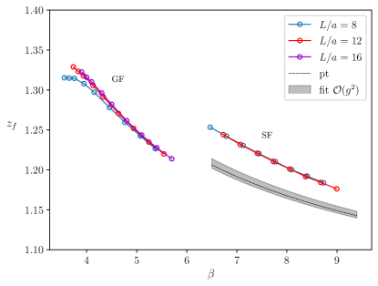
So far we have recapitulated the simulations of ref. Campos et al. (2018), performed in $N_{\mathrm{\scriptstyle f}}=3$ QCD with sea and valence quarks subjected to SF boundary conditions. In the present work, we use the same configuration ensembles, with the exception of some $\beta$’s where a few subsets of configurations could not be recovered; no significant loss in statistical accuracy resulted from this. We invert the Dirac-Wilson operator with $\chi$SF boundary conditions. Consequently $z_{\rm f}$ has to be determined so that Eq. (11) is satisfied. The results of $z_{\rm f}$ as a function of $\beta$ for both high- and low-energy regimes are displayed in Fig. 1. It should be stressed that determining $z_{\rm f}$ is essential in order to ensure that in our mixed action approach chiral and flavour symmetries are recovered in the continuum and thus the theory belongs to the same universality class as other lattice regularisations. This is corroborated by the results of Sec. IV.

Figure 1: The boundary counterterm $z_{\rm f}$ on the high energy (SF) and low energy (GF) ensembles. The black dotted line is the perturbative result known at $O(g_{0}^{2})$. The grey band is the result from fitting the SF data, plotted after the resulting expression has been truncated at $O(g_{0}^{2})$ (i.e. the fit to the data correctly reproduces the perturbative prediction).

Details of the tuning procedure leading to $z_{\rm f}$ are discussed in Appendix A. As stated in Sec. II, the tuning of $z_{\rm f}$ must in principle be coupled with that of $\kappa$ for the theory to be massless. This is not so in the procedure outlined above and in Appendix A, where we used the $\kappa_{\rm c}$ estimates of ref. Campos et al. (2018), based on the SF quark mass definition of Eq. (14). In the $\chi$SF setup the PCAC quark mass, defined by Eq. (13), is not expected to be exactly zero when $\kappa_{\rm c}$ is tuned in SF-LQCD. (The difference however is an $O(a)$ cutoff effect which induces $O(a^{2})$ corrections in ${\cal P}_{5}$-even quantities.) One would expect that an iterative procedure in which $z_{\rm f}$ and $\kappa$ are alternatively tuned would be needed. Such a procedure is adopted in Appendix B, where it is demonstrated that the tuning of $\kappa_{\rm c}$ alongside that of $z_{\rm f}$ is not necessary in practice.

The counterterm $d_{s}$, introduced in Eq.(II), is known at tree level Sint (2011) and, for the plaquette action, also at 1-loop order Dalla Brida et al. (2016a):

$$d_{s}=\frac{1}{2}+d_{s}^{(1)}g_{0}^{2}\,\,,$$ (26)

where

$$d_{s}^{(1)}=-0.0006(3)\times C_{F}\,\,.$$ (27)

For the Lüscher-Weisz action $d_{s}^{(1)}$ is not known at present. In Appendix C it is explicitly shown that results are unaffected when the 1-loop estimate of $d_{s}$ is used instead of its tree level value.

For global fits throughout this work we use the lsqfit G. P. Lepage (a) and gvar G. P. Lepage (b) packages for correlated fitting and error propagation. We have checked that these results are consistent with jackknife and the $\Gamma$-method error analysis of ref. Wolff (2004). Except for the last method, data have been binned by 20 configurations. The code to compute the $\chi$SF correlation functions is built on openQCD 1.0 and previously used in ref. Dalla Brida et al. (2019).

In order to facilitate future use of our $\chi$SF/SF-LQCD setup, we have gathered all relevant simulation details in Appendix D. These are the number of measurements $N_{\rm\scriptscriptstyle ms}$ for each ensemble, the lattice size $L/a$, the bare parameters $\beta,\kappa_{\rm c}$, the action coefficients $c_{\rm sw},z_{\rm f}$, the renormalised squared coupling $u$, and the functions $g_{\rm\scriptscriptstyle A}^{ud}$ and $\partial g_{\rm\scriptscriptstyle A}^{ud}/\partial z_{\rm f}$ used for the tuning of $z_{\rm f}$.

IV The ratio $Z_{\rm\scriptscriptstyle S}/Z_{\rm\scriptscriptstyle P}$

Now we turn to the ratio of renormalisation factors $Z_{\rm\scriptscriptstyle S}/Z_{\rm\scriptscriptstyle P}$. In Wilson formulations of lattice gauge theory, it is a finite quantity that depends on the bare gauge coupling,

$$\frac{Z_{\rm\scriptscriptstyle S}}{Z_{\rm\scriptscriptstyle P}}\simeq 1+\sum_{i=1,j=0}^{\infty}c_{ij}g_{0}^{2i}\Big{(}\frac{a}{L}\Big{)}^{2j}\,.$$ (28)

In the $g_{0}\rightarrow 0$ limit the above expression would be written as an equality, if terms containing products like $[a/L]^{2j}[\ln(a/L)]^{k}$ ($j>0,k>1$) were also added to the series; cf. Eq.(7.4) of ref. Dalla Brida et al. (2016a). We drop these terms, which are habitually neglected, as they cannot be resolved by the data. We have also ignored nonperturbative contributions depending on $a\Lambda_{\rm\scriptscriptstyle QCD}$. We use the above expression for analysing $Z_{\rm\scriptscriptstyle S}/Z_{\rm\scriptscriptstyle P}$ in the high-energy region. At a fixed bare coupling there is a finite $a/L\to 0$ limit, and for our lattice setup the leading coefficient $c_{10}$ has been calculated in lattice perturbation theory, $c_{10}=0.025944(3)$ Dalla Brida et al. (2016a).

Unlike the renormalisation factors $Z_{\rm\scriptscriptstyle S}$ and $Z_{\rm\scriptscriptstyle P}$ themselves, their ratio does not depend on the scale $\mu$. Its continuum limit is known to be unity. Moreover, it has been calculated by other methods in the low energy range for our lattice setup. Therefore it is suitable for some crosschecks of our results. Following ref. Dalla Brida et al. (2016a), we compute $Z_{\rm\scriptscriptstyle S}/Z_{\rm\scriptscriptstyle P}$ from the ratio

$$R^{g}_{\rm\scriptscriptstyle SP}\equiv\dfrac{g^{ud}_{\rm\scriptscriptstyle P}(T/2)}{ig^{uu^{\prime}}_{\rm\scriptscriptstyle S}(T/2)}=\dfrac{Z_{\rm\scriptscriptstyle S}}{Z_{\rm\scriptscriptstyle P}}+O\Big{(}\dfrac{a^{2}}{L^{2}}\Big{)}\,\,.$$ (29)

Note that $O(a)$ boundary effects cancel in this ratio, leaving us with $O(a^{2})$ uncertainties.

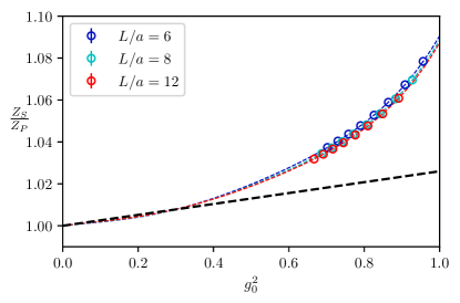
In Fig. 2 we show data for $Z_{\rm\scriptscriptstyle S}/Z_{\rm\scriptscriptstyle P}$ in the high energy regime, where contact is made with perturbation theory. Due to the high degree of statistical correlation between $g^{ud}_{\rm\scriptscriptstyle P}(x_{0})$ and $g^{uu^{\prime}}_{\rm\scriptscriptstyle S}(x_{0})$, the error bars are extremely small, of order $10^{-5}$ (as compared to $10^{-3}$ for the correlators individually). Nevertheless we are able to fit the data, performing global fits according to Eq. (28), provided enough terms in $g_{0}^{2}$ are retained. The coefficient $c_{10}$ is kept fixed at its perturbative value and the series is truncated at $(i,j)=(5,2)$. The goodness of the fit is $\chi^{2}/{\rm d.o.f.}\sim 0.68$. Thus the numerical results appear to be joining smoothly onto the one-loop perturbative result at small bare coupling. If the term $c_{10}$ is allowed to vary, the fit returns $c_{10}=0.073(57)$ and $\chi^{2}/{\rm d.o.f.}=0.66$, compatible at $1\sigma$ with the perturbative value, but only weakly constrained. The three fit results for fixed $L/a=6,8,12$ are shown as dashed lines in Fig. 2. Although they lie extremely close to each other, they are clearly distinct curves. These differences imply that finite size effects are tiny. This analysis has not been carried out along lines of constant physics; $O(a^{2}\Lambda_{\rm\scriptscriptstyle QCD}^{2})$ effects have been neglected. It therefore probes the validity of perturbative expectations in a wide range of high energy scales.

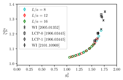
At low-energies (GF) we show results for $Z_{\rm\scriptscriptstyle S}/Z_{\rm\scriptscriptstyle P}$ in Fig. 3, and compare them with recent results obtained in de Divitiis et al. (2019) from suitable ratios of current and subtracted quark masses at two lines of constant physics (LCP-0,1) and in Heitger et al. (2020, 2021) using Ward Identities (WI). These works use the same bulk action as the present one, with Schrödinger functional boundary conditions; quark masses lie close to the chiral limit; gauge couplings straddle the range of values of CLS simulations Bruno et al. (2015); Mohler et al. (2018) suitable for the computation of low-energy hadronic quantities. Our results are compatible with those of the other methods in the infrared. The comparison of results from de Divitiis et al. (2019) and Heitger et al. (2020, 2021) was discussed already in Heitger et al. (2020, 2021), and it was observed that the WI method has smaller lattice artefacts. This can be expected to translate to an improved control of the continuum extrapolation of the quantities requiring $Z_{\rm\scriptscriptstyle S}/Z_{\rm\scriptscriptstyle P}$. Our results feature almost no visible finite volume effects and coincide numerically with the ones from Heitger et al. (2020) in the region of $g_{0}^{2}$ where they overlap. At $g_{0}^{2}$ values larger than about 1.6, different methods give slightly different results, signalling the presence of sizeable discretisation effects.

Figure 2: The ratio $Z_{\rm\scriptscriptstyle S}/Z_{\rm\scriptscriptstyle P}$ in the high energy (SF) regime. The coloured circles show our numerical data, and the coloured dotted lines show the results of the fit to Eq. (28) evaluated at the respective $L/a$ values. The black dotted line gives the $O(g_{0}^{2})$ perturbative result.

Figure 3: The ratio $Z_{\rm\scriptscriptstyle S}/Z_{\rm\scriptscriptstyle P}$ in the low energy (GF) regime. Data is compared with the results of de Divitiis et al. (2019) using quark-mass ratio methods (LCP-0,1) and Heitger et al. (2020, 2021) obtained from Ward identities (WI).

Besides the ratio $Z_{\rm\scriptscriptstyle S}/Z_{\rm\scriptscriptstyle P}$, we also examine the ratio of the corresponding SSF’s $\Sigma_{\rm\scriptscriptstyle P/S}\equiv\Sigma_{\rm\scriptscriptstyle P}/\Sigma_{\rm\scriptscriptstyle S}$. This is also a scale-independent quantity which becomes unity in the continuum limit. Once again, $O(a)$ boundary effects cancel in this ratio, leaving us with $O(a^{2})$ uncertainties. This quantity is particularly suitable for studying universality.

We use $\Sigma_{\rm\scriptscriptstyle P/S}$ in order to monitor the size of perturbative discretisation effects, making use of lattice perturbation theory to $O(g_{0}^{2})$; clearly this is meaningful only at high energy (SF) scales. We first define the ratio of the lattice SSF $\Sigma_{\rm\scriptscriptstyle P}(u,a/L)$, computed at 1-loop, to the same quantity in the $L/a=\infty$ limit, in order to determine the numerical effect of all lattice artefacts appearing at this order:

$$\frac{\Sigma_{\rm\scriptscriptstyle P}^{\rm\scriptscriptstyle 1-loop}(u,a/L)}{\sigma_{\rm\scriptscriptstyle P}^{\rm\scriptscriptstyle 1-loop}(u)}\,\,=\,\,1+u\delta_{\rm\scriptscriptstyle{P}}(a/L)\,\,,$$ (30)

$$\delta_{\rm\scriptscriptstyle{P}}(a/L)=-d_{0}\ln(2)c_{\rm\scriptscriptstyle{P}}(a/L)\,\,.$$ (31)

In the above $d_{0}=8/(4\pi)^{2}$ is the universal anomalous dimension coefficient for the pseudoscalar bilinear operator. Analogous expressions are defined for the scalar operator (same $d_{0}$). The numerical values of $c_{S,P}(a/L)$, calculated in ref. Dalla Brida et al. , are given in Table. 1.

$L/a$	$c_{\rm\scriptscriptstyle S}(a/L)$	$c_{\rm\scriptscriptstyle P}(a/L)$
6	0.1080	0.0486
8	0.0688	0.0458
12	0.0240	0.0168
16	0.0121	0.0086

Table 1: Subtraction coefficients used to remove discretisation effects from the nonperturbative step-scaling functions $\Sigma_{\rm\scriptscriptstyle{S,P}}$ up to $O(g^{2})$ as given in Eqs. (30), (31).

The lattice artefacts of $O(g_{0}^{2}a^{n})$ are subsequently subtracted from the $\Sigma_{\rm\scriptscriptstyle{S,P}}$ functions, computed nonperturbatively as in Eq. (19) and Eq. (20), according to

$$\Sigma^{\text{sub}}_{\rm\scriptscriptstyle{S,P}}(u,a/L)\equiv\frac{\Sigma_{\rm\scriptscriptstyle{S,P}}(u,a/L)}{1+u\delta_{\rm\scriptscriptstyle{S,P}}(a/L)}\,\,.$$ (32)

The remaining discretisation errors in $\Sigma^{\text{sub}}_{\rm\scriptscriptstyle{S,P}}$ are $O(g_{0}^{4}a^{2})$.

Supressing all $O(g_{0}^{2}a^{n})$ terms using lattice perturbation theory, we can in principle remove the corresponding parameters in our global fit ansatze; cf. Eq. (33). This means that we can expect more accurate determination of the remaining parameters, and more robust determinations e.g. upon increasing the order at which the expansion is truncated. Furthermore we might expect, especially at high energies where the gauge coupling is small, that removing lattice artefacts up to this order removes the largest contribution at each fixed order in $a^{n}$. This means that we may expect smaller coefficients in the remaining power series after the subtraction (i.e. the resulting power series is better behaved), although this is not guaranteed. Thus we would expect our fit forms, which are truncated to some order, to represent the subtracted data more accurately, resulting in better $\chi^{2}/\text{dof}$ and improved confidence in our extrapolated results

$$\Sigma_{\rm\scriptscriptstyle P/S}(u,a/L)=1+\sum_{i,j=1}d_{ij}u^{i}\Bigl{(}\frac{a}{L}\Bigr{)}^{2j}\,\,,$$ (33)

where terms depending on $\ln(a/L)$ are again neglected.

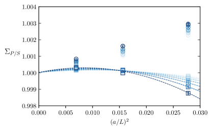
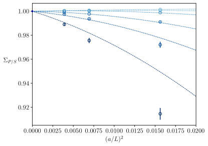
Here we test these expectations for the ratio of step-scaling functions $\Sigma_{{\rm\scriptscriptstyle P}/{\rm\scriptscriptstyle S}}$. Since the scalar and pseudoscalar bilinear operators have the same continuum anomalous dimension, the deviation of this quantity from one is a measure of lattice artefacts. For a fixed renormalised coupling $u$, the data should extrapolate to 1 in the $a/L\to 0$ limit. Fig. 4 shows $\Sigma_{{\rm\scriptscriptstyle P}/{\rm\scriptscriptstyle S}}$ vs. $(a/L)^{2}$ for the eight renormalised couplings in the high-energy (SF) regime, both before and after the subtraction specified by Eq. (32). The strong statistical correlation of $\Sigma_{\rm\scriptscriptstyle P}$ and $\Sigma_{\rm\scriptscriptstyle S}$ on a given ensemble results to extremely small statistical uncertainty, leaving systematic effects to dominate. The raw data is shown above (circles, w/out lines passing through them), with the darker colours corresponding to larger renormalised coupling. We observe that the data at smaller coupling is nearer to 1, as is expected for a “well-behaved” series at small coupling and sufficiently small lattice spacing. A fit of the data to Eq. (33) for $(i,j)=(3,2)$ gives a $\chi^{2}/{\rm d.o.f.}\sim 0.48$. Increasing $i_{\text{max}}$ or $j_{\text{max}}$ in the fit doesn’t appreciably improve the $\chi^{2}/{\rm d.o.f.}$.

The lower part of Fig. 4 gives the same data but after subtraction specified by (32), along with the curves determined by a global fit to this data. For $L/a=8$ and 12, the subtracted data is exceptionally close to 1, indicating that the $O(g_{0}^{2})$ lattice artefacts are indeed dominant. There is a more obvious discrepancy from 1 for $L/a=6$, up to around 0.001 for the $u=2.0120$ ensemble, but the overall size of this is significantly smaller than for the unsubtracted data, indicating the leading source of artefacts are still removed. Note that after subtraction the data at smaller coupling is still closer to one than the data at larger coupling. We can fit the subtracted data to the form Eq. (33), but now excluding the terms $d_{1j}$ that should be absent from the subtraction. For the same $(i,j)=(3,2)$ fit as in the unsubtracted case, we find a $\chi^{2}/{\rm d.o.f.}$ of 0.96. This is shown as the dotted lines in Fig. 4. As expected, we note that increasing $(i_{\text{max}},j_{\text{max}})$ improves the $\chi^{2}/{\rm d.o.f.}$ somewhat and that fits to the unsubtracted data using the restricted form $d_{1j}=0$ result in poor $\chi^{2}$.

The analogous study of the ratio $\Sigma_{\rm\scriptscriptstyle P}/\Sigma_{\rm\scriptscriptstyle S}$ in the low energy regime, shown in Fig. 5, does not involve any perturbative subtractions. The results reveal that higher order powers of $(a/L)^{2}$ are present, and become increasingly pronounced, at larger coupling. In fact, at our two largest couplings ($u=5.8673$ and $u=6.5489$), a low-order polynomial in $(a/L)^{2}$ has trouble capturing the behaviour, indicating that in $\Sigma_{\rm\scriptscriptstyle S}$ or $\Sigma_{\rm\scriptscriptstyle P}$ (or both) an extrapolation to the continuum value may be unreliable for the given lattice extents and couplings. The result of fitting the data to Eq. (33) for $(i_{\text{max}},j_{\text{max}})=(4,3)$ is shown in Fig. 5, which returns a $\chi^{2}/{\rm d.o.f.}$ of 4.2. Increasing $(i_{\text{max}},j_{\text{max}})$ improves the $\chi^{2}/{\rm d.o.f.}$ somewhat, but all fits studied have trouble with the $L/a=8$ points for large coupling. On the other hand the $(4,3)$ fit has $\chi^{2}/{\rm d.o.f.}=1.3/0.66$ if data from the last/second to last couplings are removed.

Figure 4: Global fit of $\Sigma_{{\rm\scriptscriptstyle P}/{\rm\scriptscriptstyle S}}$ data in the high energy (SF) regime after subtraction of $O(u,(a/L)^{n})$-effects. Data before/after subtraction are given by open circles/squares. Fit results to the subtracted data are shown as dashed lines.

Figure 5: Global fit of $\Sigma_{{\rm\scriptscriptstyle P}/{\rm\scriptscriptstyle S}}$ data in the low energy (GF) regime.

V Quark mass running at high energies

We now turn to the computation of the step-scaling functions themselves, which are the main inputs for the determination of the nonperturbative running of the quark masses. On each pair of ($L$, $2L$) ensembles we compute $\Sigma_{\rm\scriptscriptstyle P}^{\rm\scriptscriptstyle\chi SF}$, defined in Eq. (19); henceforth the superscript $\chi$SF will be dropped:

$$\Sigma_{\rm\scriptscriptstyle P}(u,a/L)=\frac{Z_{\rm\scriptscriptstyle P}(u,2L/a)}{Z_{\rm\scriptscriptstyle P}(u,L/a)}\,.$$ (34)

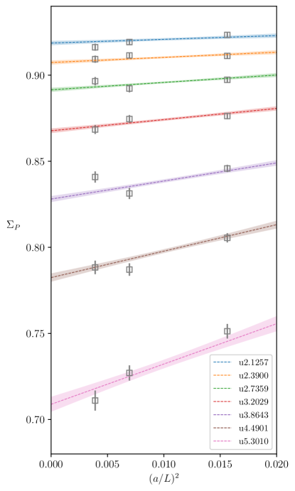
In both the high energy and low energy regimes we work at three different lattice spacings, except for the largest coupling in the high energy range (the switching point, $u=2.0120$) where we use four lattice spacings. We note here that the values of $\Sigma_{\rm\scriptscriptstyle P}$ at different couplings are statistically uncorrelated. Furthermore the numerator and denominator are uncorrelated and as a result the statistical uncertainties are significantly larger than for the quantities $\Sigma_{\rm\scriptscriptstyle P/S}$ or $Z_{\rm\scriptscriptstyle S}/Z_{\rm\scriptscriptstyle P}$ studied in Sec. IV. In order to effectively leverage the data in the high-energy (SF) regime, we carry out a global to the following form:

$$\Sigma_{\rm\scriptscriptstyle P}(u,a/L)=1+\sum_{i=1,j=0}\,b_{ij}u^{i}(a/L)^{2j}\,.$$ (35)

The continuum step-scaling function $\sigma_{\rm\scriptscriptstyle P}$ is then given by $\sigma_{\rm\scriptscriptstyle P}(u)=\lim_{a\to 0}\Sigma_{\rm\scriptscriptstyle P}(u,a/L)$. Although $\Sigma_{\rm\scriptscriptstyle P}(g_{0}^{2},a/L)$ is computed at specific values of the bare coupling and lattice volume, we are interested in its behaviour with varying renormalised coupling; hence the notation $\Sigma_{\rm\scriptscriptstyle P}(u,a/L)$.

The continuum coefficient $b_{10}=-d_{0}\ln(2)$ is known from perturbation theory, where $d_{0}=8/(4\pi)^{2}$ is the universal lowest-order quark mass anomalous dimension; see Eqs. (39) below. Also known in perturbation theory is the coefficient $b_{20}=-d_{1}\ln(2)+(d_{0}^{2}/2-b_{0}d_{0})\ln(2)^{2}$. Here $b_{0}=(11-2N_{\mathrm{\scriptstyle f}}/3)/(4\pi)^{2}$ is the universal lowest-order coefficient of the Callan-Symanzik $\beta$-function and $d_{1}=1/(4\pi)^{2}(0.2168+0.084N_{\mathrm{\scriptstyle f}})$, the NLO coefficient of the quark mass anomalous dimension, is specific to the SF scheme and was computed in Sint and Weisz (1999). For $N_{\mathrm{\scriptstyle f}}=3$ we have $b_{20}=-0.0028$. We can constrain the fit form Eq. (35) using these values. By subtracting leading $O(u)$ discretisation errors from our data (cf. Eq. (32)), we can also set the terms $b_{1j>0}$ to zero. However we find that doing so generally leads to somewhat higher $\chi^{2}/\text{dof}$ values (and is less conservative, giving smaller errors), and so we choose to work with the unsubtracted data.

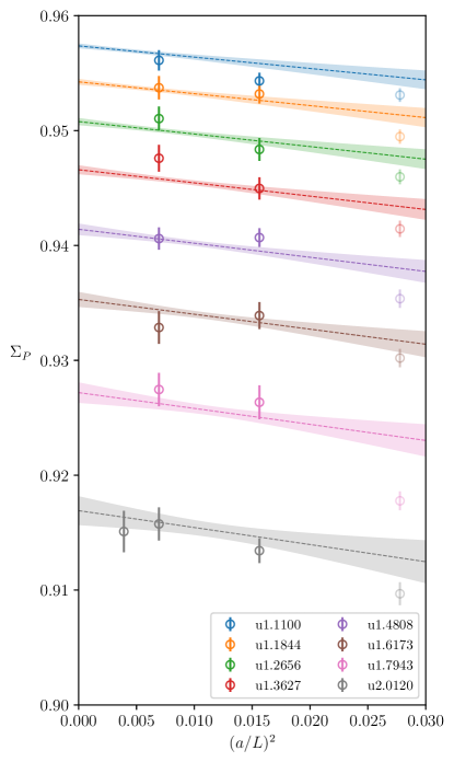
For the fits considered here we take $(i_{\text{max}},j_{\text{max}})=(3,2)$. When fitting the full dataset, we find $\chi^{2}/\text{dof}\approx 1.4$, and this is not appreciably improved by increasing $(i_{\text{max}},j_{\text{max}})$. We attribute this to a partial breakdown of the polynomial form Eq. (35) when including the $L/a=6$ points in our dataset, especially at large couplings. If we remove these points we find an improved $\chi^{2}/\text{dof}=0.95$. If we leave the term $b_{20}$ unconstrained this fit returns a value of $b_{20}=-0.0019(11)$, compatible with the perturbative value. Including the $L/a=6$ data instead gives $b_{20}=-0.0012(9)$, once again giving some evidence that the form (35) strains to represent these points. Therefore for our preferred fit we drop the $L/a=6$ data and fix $b_{20}$ to its perturbative value.

The raw step-scaling data in the high energy regime, along with the curves from the global fits evaluated at their respective $u$ values, are shown in Fig. 6.

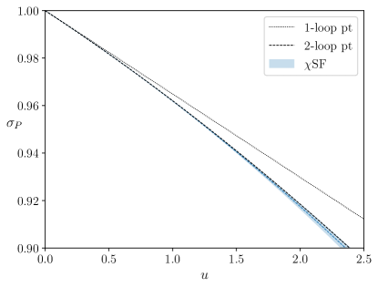
The continuum curve $\sigma_{\rm\scriptscriptstyle P}(u)$ obtained from the fit (35) is shown in Fig. 7 and compared with the expectations from perturbation theory. One sees that in the high energy region the nonperturbative result agrees well with the two-loop result from perturbation theory, indicating that the perturbative series is fairly well converged. This result is also consistent with the findings of Campos et al. (2018), and demonstrates the universality of $\chi$SF and SF.

We have established that the result shown in Fig. 7 is a robust nonperturbative estimate of $\sigma_{\rm\scriptscriptstyle P}(u)$. Having been constrained by perturbation theory at small couplings, it is also valid below the lowest simulated value $u_{\rm\scriptscriptstyle SF}\sim 1.1$. In other words, this result can be used in the whole energy range above $\mu_{0}/2\sim 2~{}$GeV, allowing us to compute the mass-evolution values $R^{(k)}$, defined as (cf. Eq.(22))

$$R^{(k)}=\frac{\kern 2.0pt\overline{\kern-1.0ptm\kern-1.0pt}\kern 1.0pt(2^{k}\mu_{0})}{\kern 2.0pt\overline{\kern-1.0ptm\kern-1.0pt}\kern 1.0pt(\mu_{0}/2)}=\prod_{n=0}^{k}\sigma_{\rm\scriptscriptstyle P}(u_{n})\,\,,$$ (36)

for arbitrarily large energy scales $2^{k}\mu_{0}$ (large $k$); in the above $u_{n}=u_{\rm\scriptscriptstyle SF}(2^{n}\mu_{0})$. For small values of $k$, Table 2 shows our results for $R^{(k)}$ from the fit to the full data set (labelled $R^{(k)}$) and those excluding the $L/a=6$ data points (labelled $R^{(k)}$-w/o $6$). The results including the $L/a=6$ data are systematically larger than those without, an effect consistent with the findings of Campos et al. (2018). As previously stated, and in accordance with ref. Campos et al. (2018), we take our preferred values to be those excluding $L/a=6$ since there is evidence that higher order discretisation effects are large for these points, and the uncertainty estimate is more conservative when excluding them. Having excluded the $L/a=6$ data from our analysis, we compute $R^{(k)}$ for increasing $k$ values, which take us beyond the energy range covered by our data. This is tenable, given that our fit is also constrained by perturbation theory at small $u$; cf. Fig. 7. The behaviour of $R^{(k)}$ with growing $k$ is displayed in Table 3, where we also show results for $M/\kern 2.0pt\overline{\kern-1.0ptm\kern-1.0pt}\kern 1.0pt(\mu_{0}/2)$ (see Eq.(37) below). We observe that $M/\kern 2.0pt\overline{\kern-1.0ptm\kern-1.0pt}\kern 1.0pt(\mu_{0}/2)$ remains constant within its error as $k$ increases.

Figure 6: Results of a global fit to the step-scaling data $\Sigma_{\rm\scriptscriptstyle P}(u,a/L)$ in the high-energy regime. The open circles give the raw data while the filled bands are the results returned from the fit at the respective $u$ values. The transparent $L/a=6$ data points are not included in the fit. The data points and the bands of the same colour are at a fixed value of the renormalised squared coupling $u$.

Figure 7: Continuum limit of the nonperturbatively determined step-scaling function $\sigma_{\rm\scriptscriptstyle P}(u)$, compared with perturbation theory. The 1-loop perturbative result is universal while the 2-loop result is specific to the $(\chi)$SF renormalisation scheme.

$k$	$u_{k}$	$R^{(k)}$-w/o 6	$R^{(k)}$	$R^{(k)}$ Campos et al. (2018)
0	2.0120	0.9169(13)	0.9191(10)	0.9165(12)
1	1.7126(31)	0.8536(19)	0.8569(16)	0.8530(17)
2	1.4939(38)	0.8031(22)	0.8070(17)	0.8025(20)
3	1.3264(38)	0.7615(24)	0.7656(19)	0.7608(21)
4	1.1936(35)	0.7263(25)	0.7307(20)	0.7257(22)
5	1.0856(32)	0.6961(25)	0.7005(20)	0.6968(24)

Table 2: Mass ratios $R^{(k)}$, obtained from nonperturbative SSF in $\chi$SF for increasing $k$-values, compared with the preferred SF fit from ref. Campos et al. (2018). The column marked $R^{(k)}$-w/o 6 gives results excluding the $L/a=6$ data points in the fit.

$k$	$u_{k}$	$R^{(k)}$-w/o 6	$M/\kern 2.0pt\overline{\kern-1.0ptm\kern-1.0pt}\kern 1.0pt(\mu_{0}/2)$
5	1.0856(32)	0.6961(25)	1.7514(63)
10	0.7503(19)	0.5899(25)	1.7519(74)
20	0.4664(8)	0.4769(22)	1.7523(81)
30	0.3392(4)	0.4136(19)	1.7522(80)
40	0.2667(3)	0.3716(17)	1.7524(80)

Table 3: Mass ratios $R^{(k)}$ and the ratio of RGI to renormalised quark mass at scale $\mu_{0}/2$, obtained from nonperturbative SSF in $\chi$SF at large $k$-values.

Finally, we can construct the running factor that takes a renormalised quark mass in our chosen ($\chi$)SF scheme at the scale $\mu_{0}/2$ to the renormalisation group invariant quark mass $M$:

$$\frac{M}{\kern 2.0pt\overline{\kern-1.0ptm\kern-1.0pt}\kern 1.0pt(\mu_{0}/2)}=\Big{[}\frac{M}{\kern 2.0pt\overline{\kern-1.0ptm\kern-1.0pt}\kern 1.0pt(2^{k}\mu_{0})}\Big{]}\,\,\Big{[}\frac{\kern 2.0pt\overline{\kern-1.0ptm\kern-1.0pt}\kern 1.0pt(2^{k}\mu_{0})}{\kern 2.0pt\overline{\kern-1.0ptm\kern-1.0pt}\kern 1.0pt(\mu_{0}/2)}\Big{]}\,.$$ (37)

The first factor on the r.h.s. can be calculated from

$$\frac{M}{\kern 2.0pt\overline{\kern-1.0ptm\kern-1.0pt}\kern 1.0pt(2^{k}\mu_{0})}=[2b_{0}\kern 1.0pt\overline{\kern-1.0ptg\kern 0.0pt}\kern 1.0pt^{2}_{{\rm SF}}(2^{k}\mu_{0})]^{-d_{0}/2b_{0}}\times\\ \exp\Bigl{\{}-\int_{0}^{\kern 1.0pt\overline{\kern-1.0ptg\kern 0.0pt}\kern 1.0pt_{{\rm SF}}(2^{k}\mu_{0})}dx\Bigl{[}\frac{\tau(x)}{\beta(x)}-\frac{d_{0}}{b_{0}x}\Bigr{]}\Bigr{\}}\,,$$ (38)

with $\tau$ and $\beta$ given by their perturbative expressions

$$\tau(x) = -x^{2}[d_{0}+d_{1}x^{2}+d_{2}x^{4}+\cdots]\,,$$ (39)

$$\beta(x) = -x^{3}[b_{0}+b_{1}x^{2}+b_{2}x^{4}+b_{3}x^{6}+\cdots]\,.$$

Specifically, we use the 2-loop result for $\tau(x)$ (i.e. $d_{0}$ and $d_{1}$ Sint and Weisz (1999)) and the 3-loop result for $\beta(x)$ (i.e. $b_{0}$, $b_{1}$, and $b_{2}$ Caswell (1974); Jones (1974); Bode et al. (2000)), supplemented by an estimate of $b_{3}$ from a fit performed in Dalla Brida et al. (2018)). The second factor is $R^{(k)}$ of Eq. (36) and it is known nonperturbatively. Having previously shown that the result and its error are practically independent of $k$, we quote for $k=10$:

$$\frac{M}{\kern 2.0pt\overline{\kern-1.0ptm\kern-1.0pt}\kern 1.0pt(\mu_{0}/2)}=1.7519(74)\,.$$ (40)

The above result agrees with the value obtained in the SF-LQCD setup of ref. Campos et al. (2018), $M/\kern 2.0pt\overline{\kern-1.0ptm\kern-1.0pt}\kern 1.0pt(\mu_{0}/2)=1.7505(89)$. This is the outcome of a detailed analysis performed by the authors, consisting of four different extrapolation procedures of the $\Sigma_{\rm\scriptscriptstyle P}(u,a/L)$ data, from which estimates of $M/\kern 2.0pt\overline{\kern-1.0ptm\kern-1.0pt}\kern 1.0pt(\mu_{0}/2)$ are extracted. Their preferred result, quoted here, is obtained from their so-called $\tau$:global–FITB* procedure, which consists in performing the continuum extrapolation of $\Sigma_{\rm\scriptscriptstyle P}(u,a/L)$ and the determination of the anomalous dimension $\tau(\kern 1.0pt\overline{\kern-1.0ptg\kern 0.0pt}\kern 1.0pt)$ simultaneously. We have also applied this procedure to our data. Outlining the method, we start by rewriting Eq.(35) as:

$$\Sigma_{\rm\scriptscriptstyle P}(u,a/L)=\sigma_{\rm\scriptscriptstyle P}(u)+\,\sum_{n=0}^{2}\rho_{n}u^{n}(a/L)^{2}\,.$$ (41)

Note that have been dropped from Eq.(35) terms of $O(a/L)^{4}$ and higher (i.e. terms with $j\geq 2$). We have also dropped terms multiplying $(a/L)^{2}$ of $O(u^{3})$ and higher (i.e. $b_{n1}$ terms with $n\geq 3$).

We write the logarithm of $\sigma_{\rm\scriptscriptstyle P}(u)$, in terms of the anomalous dimension $\tau$, as (cf. Eq. (45))

$$\ln\left(\Sigma_{\rm\scriptscriptstyle P}(u,a/L)-\sum_{n=0}^{2}\rho_{n}u^{n}(a/L)^{2}\right)=-\int_{\sqrt{u}}^{\sqrt{\sigma(u)}}{\rm d}x\,\frac{\tau(x)}{\beta(x)}\,,$$ (42)

where $\sigma(u)$ is the step scaling function of the renormalised gauge coupling; i.e. for $\kern 1.0pt\overline{\kern-1.0ptg\kern 0.0pt}\kern 1.0pt^{2}(\mu)=u$, $\sigma(u)=\kern 1.0pt\overline{\kern-1.0ptg\kern 0.0pt}\kern 1.0pt^{2}(\mu/2)$. For the integrand on the r.h.s. we use the truncated expansions of Eqs. (39), where $d_{0},d_{1},b_{0},b_{1},b_{2}$ are taken from perturbation theory and $b_{3}$ from a fit as explained above. Finally, a global fit of the $\Sigma_{\rm\scriptscriptstyle P}(u,a/L)$ data, with free fit parameters $\rho_{0},\rho_{1},\rho_{2}$ and $d_{2}$, results to a continuum expression for $\tau(u)$.

Having obtained $\tau(u)$, we can now work out directly $M/\kern 2.0pt\overline{\kern-1.0ptm\kern-1.0pt}\kern 1.0pt(\mu_{0}/2)$, using Eq.(38), with the scale $\mu_{0}/2$ in place of $2^{k}\mu_{0}$. This gives

$$\frac{M}{\kern 2.0pt\overline{\kern-1.0ptm\kern-1.0pt}\kern 1.0pt(\mu_{0}/2)}=1.7517(81)\,.$$ (43)

There is excellent agreement with the result of the first procedure, cf. Eq.(40), as well as with the SF-LQCD result of ref. Campos et al. (2018). We find this particularly encouraging, given the different philosophy of the two procedures. The first one entails a choice of $k$ in Eqs.(36) and (37), which we have taken to be $k=10$. We have checked the stability of our results for $5\lesssim k\lesssim 40$. The parametrisation of discretisation effects included $(a/L)^{4}$ contributions. In the second procedure, these were taken to be $(a/L)^{2}$. Although we could have included $(a/L)^{4}$ terms, we opted to stay as close as possible to the choices made in ref. Campos et al. (2018).

VI Quark mass running at low energies

Having computed the running factor to convert the renormalised mass at the scale $\mu_{0}/2$ to the renormalisation group invariant mass, we now turn to the computation of the running factor in the low-energy (GF) regime.

Whereas in the high-energy (SF) regime, we had lattices of extent $L/a=6,8,12$ (and $L/a=16$ at $u=2.0120$), in the GF regime our lattices have extent $L/a=8,12,16$, which should improve the continuum extrapolation. In the high energy regime we found that discretisation effects increase as the coupling is increased, and we observe a similar trend in our data in the low energy regime. It is evident from Fig. 9 that the $(a/L)^{2}$ coefficient grows with increasing coupling.

The low energy hadronic scale $\mu_{\text{had}}$ is defined by

$$u(\mu_{\text{had}})=9.25\,,$$ (44)

corresponding to a physical scale $\mu_{\text{had}}=233(8)$ MeV Bruno et al. (2017). Since the ratio of the switching scale $\mu_{0}/2\sim 2$ GeV to the hadronic scale $\mu_{\text{had}}$ is not a power of two, it is inconvenient to carry out the analysis in terms of the step scaling function $\sigma_{\rm\scriptscriptstyle P}(u)$, which only expresses the quark mass running between consecutive scales $\mu$ and $\mu/2$. It is preferable to rely on the mass anomalous dimension $\tau(g)$, related to $\sigma_{\rm\scriptscriptstyle P}(u)$ through

$$\sigma_{\rm\scriptscriptstyle P}(u)=\exp{\Bigl{[}-\int_{\sqrt{u}}^{\sqrt{\sigma(u)}}dg\frac{\tau(g)}{\beta(g)}\Bigr{]}}\,.$$ (45)

Expanding the integrand of the above equation $f(g)\equiv\tau(g)/\beta(g)$ as a power series

$$f(g)=\frac{1}{g}\sum_{k=0}f_{k}\,g^{2k}\,\,,$$ (46)

we obtain the following expression for the step scaling function:

$$\ln\sigma_{\rm\scriptscriptstyle P}(u)=-\sum_{k=0}f_{k}\int_{\sqrt{u}}^{\sqrt{\sigma(u)}}dg\,\,g^{2k-1}\,\,.$$ (47)

Unlike what we did in the high-energy regime, no input from perturbation theory is introduced in the above expression.

The lattice step scaling function $\Sigma_{\rm\scriptscriptstyle P}(u,a/L)$ is given as a series expansion in Eq. (35). This can be conveniently rearranged as

$$\Sigma_{\rm\scriptscriptstyle P}(u,a/L)=\sigma_{\rm\scriptscriptstyle P}(u)\Big{[}1+\sum_{j=1}(a/L)^{2j}\sum_{i=1}d_{ji}u^{i}\Big{]}\,\,,$$ (48)

resulting to the fit function

$$\ln[\Sigma_{\rm\scriptscriptstyle P}(u,a/L)]=\ln[\sigma_{\rm\scriptscriptstyle P}(u)]+\Big{[}\sum_{j=1}(a/L)^{2j}\sum_{i=1}d_{ji}u^{i}\Big{]}\,\,.$$ (49)

Thus the data points $\ln\Sigma_{\rm\scriptscriptstyle P}$ on the l.h.s. are to be fit by the product of the series of $\ln\sigma_{\rm\scriptscriptstyle P}$ of Eq.(47) times the double series with coefficients $d_{ji}$.

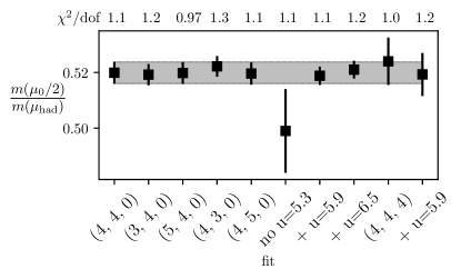
We can vary the number of coefficients $f_{k}$ parameterising the continuum form up to a value $k_{\text{max}}$. We also vary the number of coefficients $d_{ji}$ that parameterise lattice artefacts as follows: We consider artefacts that scale as $(a/L)^{2}$ as well as $(a/L)^{4}$; i.e. we set $j_{\text{max}}=2$. For each of the allowed values $j=1,2$, we vary the order of the polynomial in $u$ up to $i_{\text{max}}(j)$. Our preferred fit is the one with $k_{\text{max}}=4$, $i_{\text{max}}(1)=4$, $i_{\text{max}}(2)=0$. The fit has a $\chi^{2}/\text{dof}$ of 1.1.

We have checked the stability of our final result to changes in parameters controlling the fit form. We find good agreement in the result using different fit forms, with $\chi^{2}/\text{dof}\approx 1$, indicating our data is well-represented by and relatively insensitive to the precise details of the fit. This is shown in Fig. 8 for fit forms labelled $(k_{\text{max}},i_{\text{max}}(1),i_{\text{max}}(2))$. In addition, we can also include/exclude the data at different couplings used in the fits. The authors of Campos et al. (2018) excluded data at the two highest couplings $u=5.8673$ and $u=6.5489$. Including these couplings gives a consistent result but with somewhat smaller errors. If one instead removes the next high coupling $u=5.3010$, the data is not sufficiently constraining in the low energy region and the error increases significantly. The results from these variations are shown using our preferred (4, 4, 0) (and (4, 4, 4)) parameterisation in Fig. 8.

Figure 8: Stability analysis of the mass running factor in the low-energy regime. The leftmost point shows the result of our preferred fit (Eq. (52)). The indices $(k_{\text{max}},i_{\text{max}}(1),i_{\text{max}}(2))$ on the x-axis give the number of polynomial terms in $u$ used to parameterise the continuum, $(a/L)^{2}$, and $(a/L)^{4}$ dependences respectively. Moving from left to right, the labels ‘no $u=5.3$’, ‘$+u=5.9$’, etc. show the effect of removing/adding data at the specified couplings to our preferred (4, 4, 0) fit. The rightmost point shows the effect of adding $u=5.9$ data to the (4, 4, 4) fit.

After having fit our data for $\sigma_{\rm\scriptscriptstyle P}$ in both the SF and GF regimes and taken the continuum limit, we find at the switching scale

$$\sigma_{\rm\scriptscriptstyle P,SF}(\mu_{0}/2) =0.8951(23),$$ (50)

$$\sigma_{\rm\scriptscriptstyle P,GF}(\mu_{0}/2) =0.8941(12)\,.$$ (51)

The compatibility of these results at the threshold scale $\mu_{0}/2$, where the definition of the renormalised coupling changes, is yet another indicator of the robustness of our analysis.

Having obtained $f(g)$ from the fit and using the polynomial expression for $\beta(g)$ given in Campos et al. (2018), we can reconstruct the function $\tau$ and determine

$$\frac{\kern 2.0pt\overline{\kern-1.0ptm\kern-1.0pt}\kern 1.0pt(\mu_{0}/2)}{\kern 2.0pt\overline{\kern-1.0ptm\kern-1.0pt}\kern 1.0pt(\mu_{\text{had}})}=0.5199(39)\,,$$ (52)

which can be compared with the result from Campos et al. (2018), $\frac{\kern 2.0pt\overline{\kern-1.0ptm\kern-1.0pt}\kern 1.0pt(\mu_{0}/2)}{\kern 2.0pt\overline{\kern-1.0ptm\kern-1.0pt}\kern 1.0pt(\mu_{\text{had}})}=0.5226(43)$.

Figure 9: Results of a global fit to the step-scale data $\Sigma_{\rm\scriptscriptstyle P}$ in the low-energy regime. The open squares give the raw data while the filled bands are the results returned from the fit at the respective $u$ values. The data points close to the bands are at approximately the same $u$.

VII Conclusion

We have analysed the ensembles generated for the computation of the RG-running of the quark mass in $N_{f}=3$ massless QCD (with SF boundaries) Campos et al. (2018), imposing chirally rotated Schrödinger functional boundary conditions on the valence quarks. The data spans a few orders of magnitude, allowing a completely nonperturbative determination of the mass running function between the hadronic and very high energy scales, where contact with fixed-order perturbation theory can be made. Our computations are characterised by two different definitions of the renormalised gauge coupling below and above an energy threshold (switching scale) of $\sim 2$ GeV. This results to some differences in the computational strategies in the low- and high-energy regimes.

In order to recover all the symmetries of QCD in the continuum limit, we have performed the required nonperturbative tuning of the boundary counterterm $z_{\rm f}$ of the $\chi$SF valence quark. The critical value $\kappa_{\rm c}$ of the mass tuning parameter $\kappa$ is taken from ref. Campos et al. (2018).

We computed in both high- and low-energy regions the ratio $Z_{\rm\scriptscriptstyle S}/Z_{\rm\scriptscriptstyle P}$ and the ratio of step-scaling functions $\Sigma_{\rm\scriptscriptstyle S}/\Sigma_{\rm\scriptscriptstyle P}$. For the former we find that results match smoothly with 1-loop PT in the high energy regime. We also find consistency with determinations based on Ward identities in the low energy regime. The latter provides an important diagnostic check for the validity of our fit forms, and we find that the one-loop subtraction is effective at removing the leading lattice artefacts in this quantity. The ratio of step-scaling functions $\Sigma_{\rm\scriptscriptstyle S}/\Sigma_{\rm\scriptscriptstyle P}$ provides a second diagnostic check of our setup. The continuum limit step scaling functions $\sigma_{\rm\scriptscriptstyle S}$ and $\sigma_{\rm\scriptscriptstyle P}$ are expected to be equal in a $\chi$SF setup. We confirm that the ratio $\Sigma_{\rm\scriptscriptstyle S}/\Sigma_{\rm\scriptscriptstyle P}$ fulfils this expectation.

Our main result consists in the computation of the step-scaling function $\sigma_{\rm\scriptscriptstyle P}$ (equivalently $\tau/\beta$) from hadronic to electroweak energy scales. In the high energy regime, we computed the quark mass running factor from the switching scale to the RG-invariant definition of the quark mass. In the low energy regime, we computed the mass running factor from the hadronic scale $\mu_{\text{had}}$ to the switching scale. Putting these results together we obtain the total running factor

$$\frac{M}{\kern 2.0pt\overline{\kern-1.0ptm\kern-1.0pt}\kern 1.0pt(\mu_{\text{had}})}=0.9108(78)\,\,.$$ (53)

from eq.(40) and

$$\frac{M}{\kern 2.0pt\overline{\kern-1.0ptm\kern-1.0pt}\kern 1.0pt(\mu_{\text{had}})}=0.9107(80)\,\,.$$ (54)

from eq.(43). These can be compared to the SF-LQCD result from ref. Campos et al. (2018), namely $M/\kern 2.0pt\overline{\kern-1.0ptm\kern-1.0pt}\kern 1.0pt(\mu_{\text{had}})=0.9148(88)$, obtained on the same configuration ensembles.

Our results for the mass running factors are consistent with the findings of Campos et al. (2018). The two formulations are formally equivalent in the continuum, but are obtained from two different regularisations of the valence quark action. Their compatibility is a non-trivial check of universality of the two lattice theories.

Having validated our setup quantitatively lays the groundwork for studies of other bilinear operators, such as the tensor which, without an improvement scheme in SF, suffers $O(a)$ artefacts. Work towards obtaining automatically improved tensor matrix elements is under way; see ref. Plasencia et al. (2021b) for preliminary results. Similar advantages are expected for more complicated four-quark operators, like those used in studies of kaon mixing beyond the Standard Model. The strategy for computing automatically $O(a)$-improved $B_{\rm\scriptscriptstyle K}$ matrix elements, including BSM contributions, in a $\chi$SF renormalisation scheme, has been outlined in refs. Mainar et al. (2016); Campos et al. (2019).

Appendix A Determination of $z_{\rm f}$

To obtain “automatic” $O(a)$-improvement we tune nonperturbatively the boundary counterterm $z_{\rm f}$ in order to satisfy Eq. (11). This is done at the $\kappa_{\rm c}$ values obtained in ref. Campos et al. (2018) with SF boundary conditions for the quarks fields. We use an iterative procedure. Starting from an initial guess ($z_{\rm f}^{(0)}$, $s^{(0)}$), for $z_{\rm f}$ and $s\equiv\frac{\partial}{\partial z_{\rm f}}g_{\rm\scriptscriptstyle A}^{ud}(T/2)$, we compute $g_{\rm\scriptscriptstyle A}^{ud}(T/2)[z_{\rm f}]\equiv g_{\rm\scriptscriptstyle A}^{ud}[z_{\rm f}]$ for a given gauge field ensemble. We then update the values

$$z_{\rm f}^{(i+1)} =z_{\rm f}^{(i)}-g_{\rm\scriptscriptstyle A}^{ud}[z_{\rm f}^{(i)}]/s^{(i)}$$ (55)

$$s^{(i+1)} =(g_{\rm\scriptscriptstyle A}^{ud}[z_{\rm f}^{(i+1)}]-g_{\rm\scriptscriptstyle A}^{ud}[z_{\rm f}^{(i)}])/(z_{\rm f}^{(i+1)}-z_{\rm f}^{(i)})\,,$$ (56)

where $g_{\rm\scriptscriptstyle A}^{ud}[z_{\rm f}^{(i+1)}]$ is computed after (55) in order to update the slope in (56). As convergence criterion we require that the correlator be zero within statistical errors,

$$|g_{\rm\scriptscriptstyle A}^{ud}(T/2)|<\delta g_{\rm\scriptscriptstyle A}^{ud}(T/2)\,.$$ (57)

As an initial starting guess we take the $O(g_{0}^{2})$ perturbative result Dalla Brida et al. (2016a) for $z_{\rm f}^{(0)}=1+g_{0}^{2}C_{F}\times 0.16759(1)$. The initial guess for the slope $s^{(0)}$ was determined empirically by measuring $g_{\rm\scriptscriptstyle A}^{ud}[z_{\rm f}]$ for a few $z_{\rm f}$ values near $z_{\rm f}^{(0)}$ on a single ensemble, from which we obtained $s^{(0)}=-2.3$. In practice the slope is found to be a slowly varying function of $g_{0}^{2}$ (cf. Fig. 10) and the termination of the algorithm does not depend sensitively on its initial value. Because we are working in a narrow range around the final value of $z_{\rm f}$, the correlator $g_{\rm\scriptscriptstyle A}^{ud}[z_{\rm f}]$ varies nearly linearly with $z_{\rm f}$.

For the computation of $g_{\rm\scriptscriptstyle A}^{ud}$ the algorithm is first run in a low-precision mode using 1000 configurations, and when the convergence criterion (57) is satisfied, it switches to a high-precision mode using the full ensemble. The new starting values are the the $z_{\rm f}$- and the slope-estimates of the low-precision run. The values of $g_{\rm\scriptscriptstyle A}^{ud}[z_{\rm f}]$ for successive $z_{\rm f}$ estimates are highly correlated, so the slopes are determined precisely and the algorithm terminates quickly.

Figure 10: The slope $\frac{\partial}{\partial z_{\rm f}}g_{A}^{ud}(T/2)$ as a function of $\beta$, with varying $L/a$, in the high energy range.

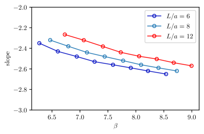
Results for both the SF and GF ensembles are shown in Fig. 1. We see that $z_{\rm f}$ varies smoothly with $g_{0}^{2}$ in each energy regime (SF and GF). Compared to the $O(g_{0}^{2})$ perturbative result, it clearly has sizeable contributions from higher orders. The results for $z_{\rm f}$ could turn out to be useful in future studies of $\chi$SF-LQCD with $N_{\mathrm{\scriptstyle f}}=3$. For this reason we present detailed results on the quantities relevant to this tuning in a separate Appendix D.

Appendix B Retuning $\kappa_{\rm c}$

The value of $\kappa_{\rm c}$ tuned in the $\chi$SF regularisation differs from the value tuned in the SF one by $O(a)$ lattice artefacts. However, when physical observables in the $\chi$SF setup are computed using these two $\kappa_{\rm c}$ values, the two determinations differ only by $O(a^{2})$ lattice artefacts Dalla Brida et al. (2016a). In this Appendix we check that physical results computed with $z_{\rm f}$ tuned with $\kappa_{\rm c}$ fixed at the SF values of ref. Campos et al. (2018) are compatible to those obtained when $z_{\rm f}$ and $\kappa_{\rm c}$ are tuned simultaneously with an iterative procedure in the $\chi$SF setup.

Our test consists in computing the SSFs of the pseudoscalar and scalar operators (19) and (20), at a single value of the renormalised coupling, $u_{\rm\scriptscriptstyle SF}(\mu_{0})$=2.012, for which an extra fine lattice with $L/a=16$ is available. Considerations based on $O(a)$-improvement in ref Dalla Brida et al. (2019) imply that the quark mass depends weakly on $z_{\rm f}$. This suggests an iterative procedure, in which either $z_{\rm f}$ or $\kappa_{\rm c}$ is tuned in alternation, while the other parameter is held fixed. The output of a tuning stage (say, $z_{\rm f}$) is thus kept fixed in the successive stage, in which the other parameter (say $\kappa_{\rm c}$) is being tuned. As we do not expect the quark mass to change appreciably with small variations of $z_{\rm f}$, the overall process should converge rapidly.

Figure 11: Simultaneous tuning of $z_{\rm f}$ and $\kappa$ at $u_{\rm\scriptscriptstyle SF}$=2.012 and lattice volume $L/a=12$. On the $x$ axis we enumerate the iteration step of the overall tuning procedure; the vertical dotted lines indicate the end of a tuning stage. Each tuning stage ends when the appropriate convergence criterion is met.

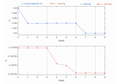
This procedure is displayed in Fig. 11. The first stage consists in tuning of $z_{\rm f}$ with $\kappa_{\rm c}$ held fixed at the SF value of ref. Campos et al. (2018). Essentially this is what is described in Appendix A. The convergence criterion is met after 3 iterations (step 3 in Fig. 11). Then the second stage begins, where $\kappa_{\rm c}$ is tuned with $z_{\rm f}$ held fixed. This is analogous to what is done in Appendix A, with $z_{\rm f}$ replaced by $\kappa_{\rm c}$: the initial guesses for $\kappa_{\rm c}$ and the slope $\frac{\partial(mL)}{\partial\kappa}$ are taken from refs. Campos et al. (2018) and Appendix B of ref. Dalla Brida et al. (2019) respectively. The algorithm first runs in low precision mode and then in high precision mode; after 3 iterations (step 6 in Fig. 11) the PCAC mass is naught within statistical precision. Note that in practice we tune the bare quark mass $m_{0}$ using the slope $\frac{\partial(mL)}{\partial(m_{0}L)}$ and then we convert it to $\kappa=\frac{1}{2m_{0}+8}$. We prefer this because $m$ is linear in $m_{0}$. See ref. Dalla Brida et al. (2019) for more details.

We can carry on by retuning $z_{\rm f}$ while keeping $\kappa_{\rm c}$ fixed to its new value; this is stage 3 of our procedure. The new initial guesses for $z_{\rm f}$ and the slope $\frac{\partial}{\partial z_{\rm f}}g_{A}^{ud}(T/2)$ are the output of the previous $z_{\rm f}$ tuning (stage 1). We alternate the two tuning procedures until both parameters remain stable within their errors.

$L/a$	$N_{conf}$	$\frac{z_{\rm f}^{\chi\rm\scriptscriptstyle{SF}}-z_{\rm f}^{\rm\scriptscriptstyle{SF}}}{z_{\rm f}^{\chi\rm\scriptscriptstyle{SF}}}\!\times\!100$	$\frac{\kappa_{\rm c}^{\chi\rm\scriptscriptstyle{SF}}-\kappa_{\rm c}^{\rm\scriptscriptstyle{SF}}}{\kappa_{\rm c}^{\chi\rm\scriptscriptstyle{SF}}}\!\times\!100$
6	5000	0.94	0.06
8	5000	0.36	0.02
12	3000	0.31	0.01
16	4604	0.19	0.005

Table 4: Percentage variation of $z_{\rm f}$ and $\kappa_{\rm c}$ (for $u_{\rm\scriptscriptstyle SF}=2.012$ ensembles) between the values tuned as in Appendix A (denoted by a superscript SF) and those tuned according to the present procedure (denoted by a superscript $\chi$SF).

Looking at the percentage variations of $z_{\rm f}$ and $\kappa_{\rm c}$ after their retuning, we see that both of them have not changed considerably: the variation of $z_{\rm f}$ is less than 1 percent for all lattice volumes and that of $\kappa_{\rm c}$ is smaller than 1 per mil. The values are given in Table 4.

Figure 12: $\Sigma_{\rm\scriptscriptstyle P}^{\rm\scriptscriptstyle\chi SF}$ vs $(a/L)^{2}$ at $u_{\rm\scriptscriptstyle SF}$=2.012. In red we show data and related fits computed with the simultaneous tuning of $z_{\rm f}$ and $\kappa_{\rm c}$; in blue, those computed w/out $\kappa_{\rm c}$ retuning.

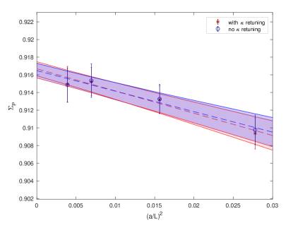
We finally compare results for $\Sigma_{\rm\scriptscriptstyle P}^{\rm\scriptscriptstyle\chi SF}$, obtained with and without retuning of $\kappa_{\rm c}$. In Fig. 12 $\Sigma_{\rm\scriptscriptstyle P}^{\rm\scriptscriptstyle\chi SF}$ is plotted against $(a/L)^{2}$ at the renormalised squared coupling $u_{\rm\scriptscriptstyle SF}$=2.012. The figure shows that the two sets of data overlap strongly, both at finite lattice spacing and in the continuum.

We conclude that the tuning procedure can be stopped after completion of the first stage (step 3 in Fig. 11), as described in Appendix A, without loss of precision for the quantities of interest.

Appendix C The effect of $d_{s}$

We compare the results for $\Sigma_{\rm\scriptscriptstyle P}^{\rm\scriptscriptstyle\chi SF}$ obtained with the tree level value of $d_{s}$ to those obtained with the 1-loop result. We perform the test at $u_{SF}$=2.0120, where the difference between the tree-level and 1-loop estimates of $d_{s}$ is the biggest possible in our high energy (SF) range: ($d_{s}^{\rm\scriptscriptstyle 1-loop}-d_{s}^{\rm\scriptscriptstyle tree})=d_{s}^{(1)}\times 2.0120=0.0016(8)$. As expected and shown in Fig. 13, the datapoints obtained with the two $d_{s}$ estimates overlap completely.

Figure 13: $\Sigma_{\rm\scriptscriptstyle P}^{\rm\scriptscriptstyle\chi SF}$vs $(a/L)^{2}$ at $u_{SF}=2.012$. In red we show data and related fits computed with $d_{s}^{\rm\scriptscriptstyle tree}$; in blue, those computed with $d_{s}^{\rm\scriptscriptstyle 1-loop}$.

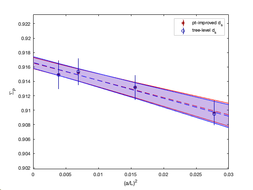
Appendix D Simulation details

$u$	$L/a$	$\beta$	$\kappa_{\rm c}$	$c_{\rm sw}$	$N_{\rm\scriptscriptstyle ms}$	$g_{\rm\scriptscriptstyle A}^{ud}$	$\partial g_{\rm\scriptscriptstyle A}^{ud}/\partial z_{\rm f}$	$z_{\rm f}$
1.110000	6	8.5403	0.13233610	1.233045285565058	5000	3.34e-07 +/- 0.000529	-2.6411749	1.18588709299
1.110000	8	8.7325	0.13213380	1.224666388699756	5000	-6.87e-07 +/- 0.000397	-2.6152159	1.18374688510
1.110000	12	8.9950	0.13186210	1.214293680665697	2769	1.89e-06 +/- 0.000348	-2.5572039	1.17624612625
1.184460	6	8.2170	0.13269030	1.248924515099129	5000	-1.33e-05 +/- 0.000571	-2.6258675	1.19427949923
1.184460	8	8.4044	0.13247670	1.239426196162344	5000	7.34e-06 +/- 0.000419	-2.5982674	1.19224223013
1.184460	12	8.6769	0.13217153	1.22701700000000	2476	1.12e-07 +/- 0.000403	-2.5383549	1.18417905314
1.265690	6	7.9091	0.13305720	1.266585617959733	5000	7.17e-06 +/- 0.000598	-2.6054349	1.20212085045
1.265690	8	8.0929	0.13283120	1.255711356539447	5000	-9.56e-07 +/- 0.000456	-2.5579952	1.20026752592
1.265690	12	8.3730	0.13249231	1.24095900000000	2729	2.36e-08 +/- 0.000400	-2.5034648	1.19163887560
1.362700	6	7.5909	0.13346930	1.288146969458134	5000	-8.57e-07 +/- 0.000656	-2.5642314	1.21157164130
1.362700	8	7.7723	0.13322830	1.275393611340024	5000	-1.20e-06 +/- 0.000485	-2.5192879	1.21009426577
1.362700	12	8.0578	0.13285365	1.25770900000000	2448	1.20e-06 +/- 0.000456	-2.4722959	1.20100624217
1.480800	6	7.2618	0.13393370	1.315030958783770	5000	1.37e-06 +/- 0.000709	-2.5311118	1.22119155568
1.480800	8	7.4424	0.13367450	1.299622821237046	5000	2.26e-06 +/- 0.000538	-2.4850676	1.22025587648
1.480800	12	7.7299	0.13326353	1.278252758659668	2711	-5.95e-07 +/- 0.000463	-2.4422897	1.21049262680
1.617300	6	6.9433	0.13442200	1.346919223092444	5000	2.77e-06 +/- 0.000786	-2.4829699	1.23119560164
1.617300	8	7.1254	0.13414180	1.327878356622864	5000	1.47e-07 +/- 0.000582	-2.4485296	1.23052937460
1.617300	12	7.4107	0.13369922	1.30220600000000	2535	4.55e-08 +/- 0.000509	-2.3828505	1.22067806449
1.794300	6	6.6050	0.13498290	1.389385004928746	5000	-2.33e-06 +/- 0.000859	-2.4255593	1.24169304397
1.794300	8	6.7915	0.13467650	1.364706438701718	5000	-1.19e-05 +/- 0.000638	-2.3657177	1.24218454960
1.794300	12	7.0688	0.13420891	1.333551296494656	2339	-7.03e-06 +/- 0.000592	-2.3034246	1.23170004013
2.012000	6	6.2735	0.13557130	1.442967721668930	5000	-8.02e-06 +/- 0.000971	-2.3627021	1.25238467445
2.012000	8	6.4680	0.13523620	1.409845308468962	5000	-3.40e-07 +/- 0.000706	-2.3251048	1.25331910626
2.012000	12	6.7299	0.13475973	1.372481791156670	3000	-1.44e-06 +/- 0.000603	-2.2547920	1.24396571640
2.012000	16	6.9346	0.13441209	1.34788873527000	4604	3.14e-06 +/- 0.000340	-2.2150346	1.23527136701

Table 5: The first column refers to the values of the squared renormalised gauge coupling $\kern 1.0pt\overline{\kern-1.0ptg\kern 0.0pt}\kern 1.0pt^{2}(\mu)=u$ in the SF energy region; columns 2 to 5 display the relevant bare lattice parameters corresponding to $u$; column 6 shows the number of gauge field configurations used for the measurements. The last three columns contain the output of the tuned $z_{\rm f}$ and the final values of $g_{\rm\scriptscriptstyle A}^{ud}$ and $\partial g_{\rm\scriptscriptstyle A}^{ud}/\partial z_{\rm f}$.

$u$	$L/a$	$\beta$	$\kappa_{\rm c}$	$c_{\rm sw}$	$N_{\rm\scriptscriptstyle ms}$	$g_{\rm\scriptscriptstyle A}^{ud}$	$\partial g_{\rm\scriptscriptstyle A}^{ud}/\partial z_{\rm f}$	$z_{\rm f}$
2.125700	8	5.3715	0.13362120	1.259364773796311	5000	4.06e-06 +/- 0.000534	-2.4642129	1.22654269651
2.125700	12	5.5431	0.13331407	1.244237155112229	2001	-1.15e-06 +/- 0.000285	-2.3724251	1.21985757706
2.125700	16	5.7000	0.13304840	1.232057931661424	8000	1.70e-06 +/- 0.000217	-2.2984404	1.21389574489
2.390000	8	5.0710	0.13421678	1.291712997425573	5000	-2.46e-06 +/- 0.000593	-2.3937509	1.24245430325
2.390000	12	5.2425	0.13387635	1.272228757209511	2001	1.77e-05 +/- 0.000311	-2.3527260	1.23476121175
2.390000	16	5.4000	0.13357851	1.256705230332892	8000	-1.26e-06 +/- 0.000261	-2.2530349	1.22758469820
2.735900	8	4.7649	0.13488555	1.335350323996506	5001	-2.82e-06 +/- 0.000687	-2.3249628	1.25947416858
2.735900	12	4.9387	0.13450761	1.308983384364439	2001	1.83e-05 +/- 0.000442	-2.2719935	1.25193714648
2.735900	16	5.1000	0.13416889	1.288203306487197	5001	-1.65e-06 +/- 0.000297	-2.1546738	1.24351820011
3.202900	8	4.4576	0.13560675	1.395741031275910	5001	6.60e-05 +/- 0.000793	-2.3080103	1.27801540556
3.202900	12	4.6347	0.13519986	1.358462476494125	2001	4.79e-06 +/- 0.000520	-2.1513773	1.27063136963
3.202900	16	4.8000	0.13482139	1.329646151978636	5001	3.06e-07 +/- 0.000360	-2.0625697	1.26149028258
3.864300	8	4.1519	0.13632589	1.482418125298923	5001	3.73e-07 +/- 0.000980	-2.1399699	1.29722920690
3.864300	12	4.3317	0.13592664	1.427424655158656	2001	-9.72e-07 +/- 0.000617	-2.0302207	1.29144247047
3.864300	16	4.5000	0.13552582	1.386110343557152	5001	-1.38e-06 +/- 0.000427	-1.9484240	1.28199124254
4.490100	8	3.9479	0.13674684	1.563885414775983	5001	1.64e-04 +/- 0.001100	-2.0493154	1.30786594013
4.490100	12	4.1282	0.13640300	1.490702297580152	2001	-1.31e-05 +/- 0.000713	-1.9429389	1.30582505718
4.490100	16	4.3000	0.13600821	1.436199798821361	5001	-1.53e-05 +/- 0.000493	-1.8420700	1.29622706156
5.301000	8	3.7549	0.13701929	1.668369108400627	5001	-8.19e-06 +/- 0.001380	-1.9545399	1.31461240780
5.301000	12	3.9368	0.13679805	1.569056010619204	2001	2.31e-05 +/- 0.000831	-1.8037352	1.31770290718
5.301000	16	4.1000	0.13647301	1.500935714848465	5001	-2.01e-05 +/- 0.000717	-1.7111716	1.31005410303
5.867300	8	3.6538	0.13707221	1.738234164347418	5001	-3.05e-05 +/- 0.001560	-1.8809782	1.31487229203
5.867300	12	3.8333	0.13696774	1.621966539608638	5001	5.56e-05 +/- 0.000921	-1.7457623	1.32327345473
5.867300	16	4.0000	0.13668396	1.540714371185832	4602	-2.24e-05 +/- 0.000654	-1.6560183	1.31588724381
6.548900	8	3.5565	0.13703245	1.818951161611082	5001	-3.29e-05 +/- 0.001830	-1.8016743	1.31531748561
6.548900	12	3.7354	0.13708263	1.680901952205217	5001	2.42e-06 +/- 0.001080	-1.6027921	1.32886731276
6.548900	16	3.9000	0.13687202	1.586881030973021	4600	-5.17e-07 +/- 0.000737	-1.5210420	1.32248784097

Table 6: The first column refers to the values of the squared renormalised gauge coupling $\kern 1.0pt\overline{\kern-1.0ptg\kern 0.0pt}\kern 1.0pt^{2}(\mu)=u$ in the GF energy region; columns 2 to 5 display the relevant bare lattice parameters corresponding to $u$; column 6 shows the number of gauge field configurations used for the measurements. The last three columns contain the output of the tuned $z_{\rm f}$ and the final values of $g_{\rm\scriptscriptstyle A}^{ud}$ and $\partial g_{\rm\scriptscriptstyle A}^{ud}/\partial z_{\rm f}$.

References

- de Divitiis et al. (2019) G. M. de Divitiis, P. Fritzsch, J. Heitger, C. C. Köster, S. Kuberski, and A. Vladikas (ALPHA), Eur. Phys. J. C79, 797 (2019), eprint 1906.03445.
- Heitger et al. (2020) J. Heitger, F. Joswig, and A. Vladikas (ALPHA), Eur. Phys. J. C 80, 765 (2020), eprint 2005.01352.
- Heitger et al. (2021) J. Heitger, F. Joswig, P. L. J. Petrak, and A. Vladikas, Eur. Phys. J. C 81, 606 (2021), eprint 2101.10969.
- Campos et al. (2018) I. Campos, P. Fritzsch, C. Pena, D. Preti, A. Ramos, and A. Vladikas, Eur. Phys. J. C78, 387 (2018), eprint 1802.05243.
- Sint (2011) S. Sint, Nucl. Phys. B847, 491 (2011), eprint 1008.4857.
- Lüscher et al. (1996) M. Lüscher, S. Sint, R. Sommer, and P. Weisz, Nucl. Phys. B478, 365 (1996), eprint hep-lat/9605038.
- Dalla Brida et al. (2016a) M. Dalla Brida, S. Sint, and P. Vilaseca, JHEP 08, 102 (2016a), eprint 1603.00046.
- Sint and Leder (2010) S. Sint and B. Leder, PoS LATTICE2010, 265 (2010), eprint 1012.2500.
- Sommer (1994) R. Sommer, Nucl. Phys. B 411, 839 (1994), eprint hep-lat/9310022.
- Lopez et al. (2013a) J. Lopez, K. Jansen, D. Renner, and A. Shindler, Nucl. Phys. B 867, 567 (2013a), eprint 1208.4591.
- Lopez et al. (2013b) J. Lopez, K. Jansen, D. Renner, and A. Shindler, Nucl. Phys. B 867, 609 (2013b), eprint 1208.4661.
- Capitani et al. (1999) S. Capitani, M. Lüscher, R. Sommer, and H. Wittig, Nucl. Phys. B 544, 669 (1999), [Erratum: Nucl.Phys.B 582, 762–762 (2000)], eprint hep-lat/9810063.
- Dalla Brida et al. (2019) M. Dalla Brida, T. Korzec, S. Sint, and P. Vilaseca, Eur. Phys. J. C79, 23 (2019), eprint 1808.09236.
- Dimopoulos et al. (2008) P. Dimopoulos, G. Herdoiza, F. Palombi, M. Papinutto, C. Pena, A. Vladikas, and H. Wittig (ALPHA), JHEP 05, 065 (2008), eprint 0712.2429.
- Dimopoulos et al. (2018) P. Dimopoulos, G. Herdoíza, M. Papinutto, C. Pena, D. Preti, and A. Vladikas (ALPHA), Eur. Phys. J. C 78, 579 (2018), eprint 1801.09455.
- Dimopoulos et al. (2009) P. Dimopoulos, H. Simma, and A. Vladikas, JHEP 07, 007 (2009), eprint 0902.1074.
- Mainar et al. (2016) P. V. Mainar, M. Dalla Brida, and M. Papinutto, PoS LATTICE2015, 252 (2016).
- Campos et al. (2019) I. Campos, M. Dalla Brida, G. M. de Divitiis, A. Lytle, M. Papinutto, and A. Vladikas, in 37th International Symposium on Lattice Field Theory (2019), eprint 1910.01898.
- Plasencia et al. (2021a) I. C. Plasencia, M. D. Brida, G. M. de Divitiis, A. Lytle, M. Papinutto, L. Pirelli, and A. Vladikas, in 38th International Symposium on Lattice Field Theory (2021a), eprint 2111.15384.
- Frezzotti and Rossi (2004) R. Frezzotti and G. Rossi, JHEP 08, 007 (2004), eprint hep-lat/0306014.
- Sint (2007) S. Sint, in Workshop on Perspectives in Lattice QCD (2007), eprint hep-lat/0702008.
- Dalla Brida et al. (2016b) M. Dalla Brida, P. Fritzsch, T. Korzec, A. Ramos, S. Sint, and R. Sommer (ALPHA), Phys. Rev. Lett. 117, 182001 (2016b), eprint 1604.06193.
- Dalla Brida et al. (2017) M. Dalla Brida, P. Fritzsch, T. Korzec, A. Ramos, S. Sint, and R. Sommer (ALPHA), Phys. Rev. D 95, 014507 (2017), eprint 1607.06423.
- Dalla Brida et al. (2018) M. Dalla Brida, P. Fritzsch, T. Korzec, A. Ramos, S. Sint, and R. Sommer (ALPHA), Eur. Phys. J. C 78, 372 (2018), eprint 1803.10230.
- Lüscher et al. (1992) M. Lüscher, R. Narayanan, P. Weisz, and U. Wolff, Nucl. Phys. B 384, 168 (1992), eprint hep-lat/9207009.
- Luscher et al. (1994) M. Luscher, R. Sommer, P. Weisz, and U. Wolff, Nucl. Phys. B 413, 481 (1994), eprint hep-lat/9309005.
- Fritzsch and Ramos (2013) P. Fritzsch and A. Ramos, JHEP 10, 008 (2013), eprint 1301.4388.
- Bruno et al. (2017) M. Bruno, M. Dalla Brida, P. Fritzsch, T. Korzec, A. Ramos, S. Schaefer, H. Simma, S. Sint, and R. Sommer (ALPHA), Phys. Rev. Lett. 119, 102001 (2017), eprint 1706.03821.
- Wilson (1974) K. G. Wilson, Phys. Rev. D 10, 2445 (1974).
- Sheikholeslami and Wohlert (1985) B. Sheikholeslami and R. Wohlert, Nucl. Phys. B 259, 572 (1985).
- Yamada et al. (2005) N. Yamada et al. (JLQCD, CP-PACS), Phys. Rev. D 71, 054505 (2005), eprint hep-lat/0406028.
- Sint and Weisz (1997) S. Sint and P. Weisz, Nucl. Phys. B 502, 251 (1997), eprint hep-lat/9704001.
- Bode et al. (1999) A. Bode, U. Wolff, and P. Weisz (Alpha), Nucl. Phys. B 540, 491 (1999), eprint hep-lat/9809175.
- Lüscher and Weisz (1985) M. Lüscher and P. Weisz, Phys. Lett. B 158, 250 (1985).
- Bulava and Schaefer (2013) J. Bulava and S. Schaefer, Nucl. Phys. B 874, 188 (2013), eprint 1304.7093.
- (36) P. Vilaseca, private communication.
- Aoki et al. (1999) S. Aoki, R. Frezzotti, and P. Weisz, Nucl. Phys. B 540, 501 (1999), eprint hep-lat/9808007.
- G. P. Lepage (a) G. P. Lepage, lsqfit (version 11.7), URL https://github.com/gplepage/lsqfit.
- G. P. Lepage (b) G. P. Lepage, gvar (version 11.9.1), URL https://github.com/gplepage/gvar.
- Wolff (2004) U. Wolff, Comput. Phys. Commun. 156, 143 (2004), [Erratum: Comput. Phys. Commun.176,383(2007)], eprint hep-lat/0306017.
- Bruno et al. (2015) M. Bruno et al., JHEP 02, 043 (2015), eprint 1411.3982.
- Mohler et al. (2018) D. Mohler, S. Schaefer, and J. Simeth, EPJ Web Conf. 175, 02010 (2018), eprint 1712.04884.
- (43) M. Dalla Brida, A. Mellini, M. Papinutto, F. Scardino, and P. Vilaseca (ALPHA), in preparation.
- Sint and Weisz (1999) S. Sint and P. Weisz (ALPHA), Nucl. Phys. B 545, 529 (1999), eprint hep-lat/9808013.
- Caswell (1974) W. E. Caswell, Phys. Rev. Lett. 33, 244 (1974).
- Jones (1974) D. R. T. Jones, Nucl. Phys. B 75, 531 (1974).
- Bode et al. (2000) A. Bode, P. Weisz, and U. Wolff (ALPHA), Nucl. Phys. B 576, 517 (2000), [Erratum: Nucl.Phys.B 608, 481–481 (2001), Erratum: Nucl.Phys.B 600, 453–453 (2001)], eprint hep-lat/9911018.
- Plasencia et al. (2021b) I. C. Plasencia, M. D. Brida, G. M. de Divitiis, A. Lytle, M. Papinutto, L. Pirelli, and A. Vladikas, in 38th International Symposium on Lattice Field Theory (2021b), eprint 2111.15325.