Implicit Extensions of an Explicit Multirate Runge–Kutta Scheme

Abstract

We propose a new method that extends conservative explicit multirate methods to implicit explicit-multirate methods. We develop extensions of order one and two with different stability properties on the implicit side. The method is suitable for time-stepping adaptive mesh refinement PDE discretizations with different degrees of stiffness. A numerical example with an advection-diffusion problem illustrates the new method’s properties.

1 Introduction

Multirate time-stepping methods have become popular in solving computational fluid dynamics problems with adaptive meshes [1, 2, 3]. Explicit multirate methods are particularly efficient at integrating partial differential equations (PDE)s with adaptive mesh refinement (AMR), where local time stepping overcomes the global Courant–Friedrichs–Lewy (CFL) limitation [4]. If these problems have stiff components, however, using purely explicit methods is inefficient or impractical. This situation forces one to use implicit-explicit (IMEX) methods; however, existing IMEX conservative methods treat the explicit component with the same global time step, which limits the time step due to the fastest component—typically, associated with the finest grid points or elements. This restriction leads to ineffective time stepping especially when one uses AMR for stiff problems. While general frameworks have been proposed (e.g., [5]), little work has been done on methods that are suitable for such conditions and also preserve linear invariants.

In this work we propose an extension to explicit multirate methods with a computationally efficient implicit component, which allows multirate treatment of the explicit component and implicitness for stiff components. The stiff components are treated with a single rate. We consider the following initial value problem: $\dot{y}(t)=F(y(t))=f(y(t))+g(y(t))\,,~{}t_{0}\leq t\leq t_{F}\,,~{}y(t_{0})=y_{0}\,.$ Here $y\in\mathbb{R}^{N}$, and $F$ typically represents the spatial discretization and can be additively partitioned into $f,g:\mathbb{R}^{N}\rightarrow\mathbb{R}^{N}$, which are Lipschitz continuous functions. We assume that $f$ is a nonstiff component that can be efficiently integrated with an explicit integrator and $g$ is a component that can be stiff and requires an implicit integrator. We further assume that the solution $y$ can be partitioned in non-overlapping subdomains, where the dynamic behavior with respect to $f$ is different. The explicit stability requirements for each subdomain are separated in different classes called levels—a reference to AMR. Therefore, we consider a component partitioning $y^{\top}=[y^{F},y^{S}]$ and the same for the explicit components $f^{\top}=[f^{F},f^{S}]$ so that the partitioned system to be solved takes the following form,

$$\begin{bmatrix}\dot{y}^{F}\\ \dot{y}^{S}\end{bmatrix}=\begin{bmatrix}f^{F}\left(y^{F},y^{S}\right)\\ f^{S}\left(y^{F},y^{S}\right)\end{bmatrix}+g\left(y\right)\,,$$ (1)

where the superscript $F$ refers to the fast component and superscript $S$ to the slow component. For brevity we consider only two partitions here; but, in general, multiple partitions can be accommodated, which are relevant for practical multiple-level adaptive mesh refinement.

A class of conservative multirate explicit partitioned Runge–Kutta (MPRK) methods was introduced in [6]. These methods are constructed by using a base method and can attain second-order overall accuracy if the base method is at least second order. In this work we extend a particular MPRK method by adding an implicit stage to handle stiff additive partitions along with the original explicit multirate scheme, while maintaining conservation at the temporal discrete level. In the PDE case, so long as the spatial discretization is conservative, the time-marched solution with the proposed method is also conserved.

The rest of the paper is organized as follows. Section 2 introduces MPRK and the notation. We provide the new method design and specific examples in Sec. 3. We illustrate the properties of the newly introduced methods in Sec. 4 through numerical examples. We provide concluding remarks in Sec. 5.

2 MPRK Methods

The multirate explicit partitioned Runge–Kutta scheme as introduced in [6] is constructed by using a base method that is repeated $m$ times with a fractional time step. The base method is defined as a classical RK method by coefficients $A=[a_{i,j}]$, $b=[b_{i}]$, and $c=[c_{i}]=A\mathbbm{1}_{s}$, where $\mathbbm{1}_{s}$ is a vector of ones of length $s$ and $i,j=1,\dots,s$ and represented in a tableau, $\begin{array}[]{c|c}\rule[-5.50003pt]{0.0pt}{18.00005pt}c&A\\ \hline\cr\rule[-5.50003pt]{0.0pt}{18.00005pt}&b^{\top}\end{array}$. In order to preserve numerical stability and conservation properties, the fast or the subcycled ($m$ times) component that corresponds to the fast partition is a repeated application of the base method with a time step of $\frac{\Delta t}{m}$; we refer to $m$ as the multirate ratio. The region around the boundary between fast and slow regions is called a buffer, with a size that depends on the spatial discretization (stencil and rate), and is typically small relative to the fast and slow regions. In the buffer region one simply repeats the base method $m$ times with $\Delta t$, leading to the slow method so that both the slow and the fast methods have the same number of stages. Then, inside the slow region, the slow method simply reverts to the base method. Efficiency gains result from applying a small time step on the fast regions and large steps on the slow regions. By construction, the fast method has a factor of $m$ more stages than the slow method on the slow method has and a fraction step size, $\Delta t/m$. For multiple refinement levels, one can use telescoping nesting, which is achieved by replacing the base method with the fast method and repeating the procedure above.

A fast-slow method can be represented as a partitioned RK:

$$Y^{F}_{i}= y^{F}_{n}+\Delta t\sum\nolimits_{j=1}^{i-1}a^{F}_{ij}f^{F}\left(Y^{F}_{j},Y^{S}_{j}\right)\,,~{}i=1,\dots,s$$ (2a)

$$Y^{S}_{i}= y^{S}_{n}+\Delta t\sum\nolimits_{j=1}^{i-1}a^{S}_{ij}f^{S}\left(Y^{F}_{j},Y^{S}_{j}\right)\,,~{}i=1,\dots,s$$ (2b)

$$y_{n+1}= y_{n}+\Delta t\sum\nolimits_{i=1}^{s}b_{i}f(Y_{i})\,,$$ (2c)

where the stages are partitioned as the solution in two fast and slow components, $Y_{i}^{\top}=[Y^{F}_{i},Y^{S}_{i}]$ and $f(Y_{i})^{\top}=[f^{F}\left(Y^{F}_{i},Y^{S}_{i}\right),f^{S}\left(Y^{F}_{i},Y^{S}_{i}\right)]$. We also set $b^{F}=b^{S}=b$, which is required for conservation. This results in the short form of (2c), where each component is computed by $y_{n+1}^{\{F,S\}}=y_{n}^{\{F,S\}}+\Delta t\sum\nolimits_{i=1}^{s}b_{i}^{\{F,S\}}f^{\{F,S\}}(Y^{F}_{i},Y^{S}_{i})$. The step size is controlled by the $a^{\{F,S\}}$ coefficients.

An example with $m=2$ is

$$\begin{array}[]{c|cc}\rule[-5.50003pt]{0.0pt}{18.00005pt}0&0\\ \rule[-5.50003pt]{0.0pt}{18.00005pt}1&1&0\\ \hline\cr\rule[-5.50003pt]{0.0pt}{18.00005pt}&\frac{1}{2}&\frac{1}{2}\\ \end{array}\qquad\begin{array}[]{c|cccc}\rule[-5.50003pt]{0.0pt}{18.00005pt}0&0\\ \rule[-5.50003pt]{0.0pt}{18.00005pt}1&1&0\\ \rule[-5.50003pt]{0.0pt}{18.00005pt}0&0&0&0\\ \rule[-5.50003pt]{0.0pt}{18.00005pt}1&0&0&1&0\\ \hline\cr\rule[-5.50003pt]{0.0pt}{18.00005pt}&\frac{1}{4}&\frac{1}{4}&\frac{1}{4}&\frac{1}{4}\\ \end{array}\qquad\begin{array}[]{c|cccc}\rule[-5.50003pt]{0.0pt}{18.00005pt}0&0\\ \rule[-5.50003pt]{0.0pt}{18.00005pt}\frac{1}{2}&\frac{1}{2}&0\\ \rule[-5.50003pt]{0.0pt}{18.00005pt}\frac{1}{2}&\frac{1}{4}&\frac{1}{4}&0\\ \rule[-5.50003pt]{0.0pt}{18.00005pt}1&\frac{1}{4}&\frac{1}{4}&\frac{1}{2}&0\\ \hline\cr\rule[-5.50003pt]{0.0pt}{18.00005pt}&\frac{1}{4}&\frac{1}{4}&\frac{1}{4}&\frac{1}{4}\\ \end{array}\,,$$ (16)

where the tableaux represent the base ($a_{ij},b_{i},c_{i}$), the slow method ($a^{S}_{ij},b^{S}_{i},c^{S}_{i}$), and the fast method ($a^{F}_{ij},b^{F}_{i},c^{F}_{i}$). In the fast region, the 4-stage fast method is used; and in the buffer and slow regions, the slow method is used. In the slow region, however, the slow method is equivalent to the 2-stage base method, and hence the computational savings is relative to having a global time step. The fast method is the result of applying the base method twice with a step size of $\Delta t/2$; therefore the fast method takes takes twice as many half-steps as the slow method takes. This particular method is the focus of our study here. The reader is referred to [6] and a recent algorithmic presentation in [7] for a more in-depth description of these methods.

3 Extended MPRK-Implicit Methods

We now introduce a three-way partitioning of (2) into explicit fast, explicit slow, and implicit stiff. We restrict the presentation to two levels; however, the explicit component of the method can be extended to arbitrary nesting levels in the same fashion as discussed above, while maintaining a fixed ratio. The resulting scheme is now described by three sets of coefficients: superscripts $F$, $S$, and $\tilde{}$ define the fast, slow, and implicit coefficients, respectively. We have two goals: ($i$) minimize the number of implicit stages and ($ii$) accommodate multiple levels of refinement, that is, telescoping nesting. To accomplish both and to avoid the loss of conservation, we will modify only the last stage in (2), which will be common across all partitions. Therefore, the last stage and the step completion in (2) become

$$Y_{s}= y_{n}+\Delta t\sum_{j=1}^{s-1}\begin{bmatrix}a^{F}_{sj}f^{F}\left(Y_{j}\right)\\ \rule[-5.50003pt]{0.0pt}{18.00005pt}a^{S}_{sj}f^{S}\left(Y_{j}\right)\end{bmatrix}+\Delta t\sum_{j=1}^{s}\tilde{a}_{sj}g\left(Y_{j}\right)$$ (17a)

$$y_{n+1}= y_{n}+\Delta t\sum_{i=1}^{s}b_{i}\left(f(Y_{i})+g(Y_{i})\right)\,.$$ (17b)

The implicit component will have only one implicit stage regardless of the number of explicit partitions and of the ratio among them. Therefore, the methods introduced here are neither multirate implicit [8] nor multirate IMEX [9]. The Butcher tableau representation of the implicit component indexed by $\tilde{a}$ as a matrix will therefore be all zeros except in the last stage and can augment the tableaux in (16). With the $b$ vector fixed, the choice of $\tilde{a}_{sj}$, $j=1,\dots,s$ is driven by stability and lastly by accuracy considerations.

We analyze stability by considering the following problem, $\dot{y}=\lambda^{F}y+\lambda^{S}y+\lambda^{\textnormal{stiff}}y$, with $\lambda^{\{F,S,\textnormal{stiff}\}}\in\mathbb{C}$ resulting from linear operators that can be diagonalized simultaneously, where each component on the right-hand side is time-stepped with the respective fast, slow, and implicit integrators. The stability function is defined by $R(z)$, $z=\lambda\Delta t$ that satisfies $y_{[n+1]}=R(z)y_{n}$. Individually, the stability of the fast method is $m$ times larger than that of the slow method. More complex stability analyses are possible, in particular if interpolation is needed [10]. In general, simplifying assumptions have to be made in all cases; however, they tend to hold well in practice.

3.1 A-Stable Second-Order Extensions

A multirate-explicit A-stable-implicit method that is second-order explicit and second-order implicit A-stable is obtained by setting $\tilde{a}_{sj}=\frac{1}{2}$, $j=1,\dots,s$ in (17). The resulting stability function of the implicit method is $R(z)=\frac{2+z}{2-z}$, which implies that the implicit part is A-stable with $R(\infty)=-1$. By using these coefficients we guarantee that the implicit-explicit stability function damps large eigenvalues; see [11, Sec 4.5]. The abscissa of the implicit method becomes $\tilde{c}=[0,0,\dots,0,m]^{\top}$ on the fast and slow parts and $\tilde{c}=[0,1]^{\top}$ for the base method. In both cases $\tilde{c}b=\frac{1}{2}$, which gives second order of the implicit part and of the overall method. Computationally the implicit part has only one implicit stage, with the rest of the stage coefficients being zero. The resulting method can be expressed in the same fashion as MPRK by augmenting the following tableaux to (16):

$$\begin{array}[]{c|cc}\rule[-5.50003pt]{0.0pt}{18.00005pt}0&0\\ \rule[-5.50003pt]{0.0pt}{18.00005pt}1&\frac{1}{2}&\frac{1}{2}\\ \hline\cr\rule[-5.50003pt]{0.0pt}{18.00005pt}&\frac{1}{2}&\frac{1}{2}\\ \end{array}\qquad\begin{array}[]{c|cccc}\rule[-5.50003pt]{0.0pt}{18.00005pt}0&0\\ \rule[-5.50003pt]{0.0pt}{18.00005pt}0&0&0\\ \rule[-5.50003pt]{0.0pt}{18.00005pt}0&0&0&0\\ \rule[-5.50003pt]{0.0pt}{18.00005pt}2&\frac{1}{2}&\frac{1}{2}&\frac{1}{2}&\frac{1}{2}\\ \hline\cr\rule[-5.50003pt]{0.0pt}{18.00005pt}&\frac{1}{4}&\frac{1}{4}&\frac{1}{4}&\frac{1}{4}\\ \end{array}\,,$$ (26)

where the first tableau corresponds to the base method and the second tableau to the slow and fast methods in (16). In particular such a method corresponds to the following algorithm:

$$Y^{F}_{1}= y^{F}_{n}\,,\qquad Y^{S}_{1}=y^{S}_{n}$$

$$Y^{F}_{2}= y^{F}_{n}+\frac{\Delta t}{2}f^{F}\left(Y^{F}_{1},Y^{S}_{1}\right)\,,\qquad Y^{S}_{2}=y^{S}_{n}+\Delta tf^{S}\left(Y^{F}_{1},Y^{S}_{1}\right)\,,$$

$$Y^{F}_{3}= y^{F}_{n}+\frac{\Delta t}{4}f^{F}\left(Y^{F}_{1},Y^{S}_{1}\right)+\frac{\Delta t}{4}f^{F}\left(Y^{F}_{2},Y^{S}_{2}\right)\,,\qquad Y^{S}_{3}=y^{S}_{n}\,,$$

$${\color[rgb]{1,0,0}Y_{4}}= y_{n}+\Delta t\begin{bmatrix}\frac{1}{4}f^{F}\left(Y^{F}_{1},Y^{S}_{1}\right)+\frac{1}{4}f^{F}\left(Y^{F}_{2},Y^{S}_{2}\right)+\frac{1}{2}f^{F}\left(Y^{F}_{3},Y^{S}_{3}\right)\\ \rule[-5.50003pt]{0.0pt}{18.00005pt}f^{S}\left(Y^{F}_{3},Y^{S}_{3}\right)\end{bmatrix}+$$

$$\quad\frac{\Delta t}{2}\left(g(Y_{1})+g(Y_{2})+g(Y_{3})+g({\color[rgb]{1,0,0}Y_{4}})\right)\,,$$

$$y_{n+1}= y_{n}+\frac{\Delta t}{4}\sum_{i=1}^{4}\left(f(Y_{i})+g(Y_{i})\right)\,,$$

where the terms in red illustrate the sole implicit components.

3.2 L-Stable First-Order Extensions

Partitioned methods of type (2), (17) with one implicit stage cannot be both second order and L-stable at the same time because of the constraints imposed on the order conditions and the stability function. Thus, L-stable implicit methods coupled to the multirate method can be at most second order accurate on the explicit part and first order on the implicit part. One such method is obtained by choosing $\tilde{a}_{sj}=1$, $j=1,\dots,s$ in (17). The resulting stability function of the implicit method is $R(z)=\frac{1}{1-z}$. The abscissa of the implicit method corresponds to $\tilde{c}=[0,0,\dots,0,m\,s]^{\top}$ on the fast and slow parts and $\tilde{c}=[0,s]^{\top}$ for the base method and $\tilde{c}b=\frac{1}{2}=1$. Therefore, this multirate-IMEX method is second-order explicit and first-order implicit L-stable. As in the case above, the resulting method can be expressed in the same fashion as MPRK by augmenting the following tableaux to (16):

$$\begin{array}[]{c|cc}\rule[-5.50003pt]{0.0pt}{18.00005pt}0&0\\ \rule[-5.50003pt]{0.0pt}{18.00005pt}2&1&1\\ \hline\cr\rule[-5.50003pt]{0.0pt}{18.00005pt}&\frac{1}{2}&\frac{1}{2}\\ \end{array}\qquad\begin{array}[]{c|cccc}\rule[-5.50003pt]{0.0pt}{18.00005pt}0&0\\ \rule[-5.50003pt]{0.0pt}{18.00005pt}0&0&0\\ \rule[-5.50003pt]{0.0pt}{18.00005pt}0&0&0&0\\ \rule[-5.50003pt]{0.0pt}{18.00005pt}4&1&1&1&1\\ \hline\cr\rule[-5.50003pt]{0.0pt}{18.00005pt}&\frac{1}{4}&\frac{1}{4}&\frac{1}{4}&\frac{1}{4}\\ \end{array}\,,$$ (35)

where the first tableau corresponds to the base method and the second tableau to the slow and fast methods in (16).

4 Numerical Examples

We illustrate the properties of the methods introduced above by using a one-dimensional advection-diffusion problem,

$$\frac{\partial{u(t,x)}}{\partial{t}}+\frac{\partial}{\partial{x}}\left(\omega(x)u(t,x)\right)=\delta\,\frac{\partial^{2}{u(t,x)}}{\partial{x}^{2}}\,,$$ (36)

Figure 1: Flux function ($m=2$ & $m=4$)

which is discretized in space in $M$ uniform intervals. This leads to a semi-discrete system $y(t)=\{u_{k}(t)\}_{k=1,\dots,M}$. We discretize the advective term by using a conservative third-order upwind-biased finite difference method and the diffusive term by second-order finite differences, and we use periodic boundary conditions. The numerical stability restriction in the advective term is adjusted by using different values of $\omega$ in space to mimic AMR (Fig. 1), where we consider two cases suitable for $m=2$ and $m=4$. The stiffness is controlled by changing the value of $\delta$. The time step is kept the same for all simulations. Advection is treated explicitly with different rates and diffusion implicitly with a single-rate integrator.

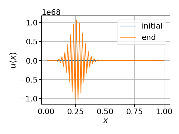
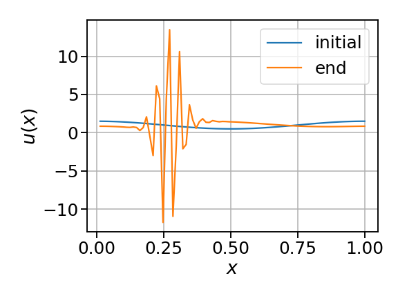
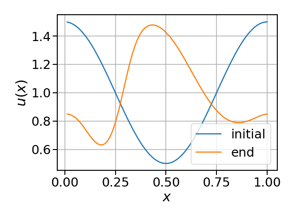
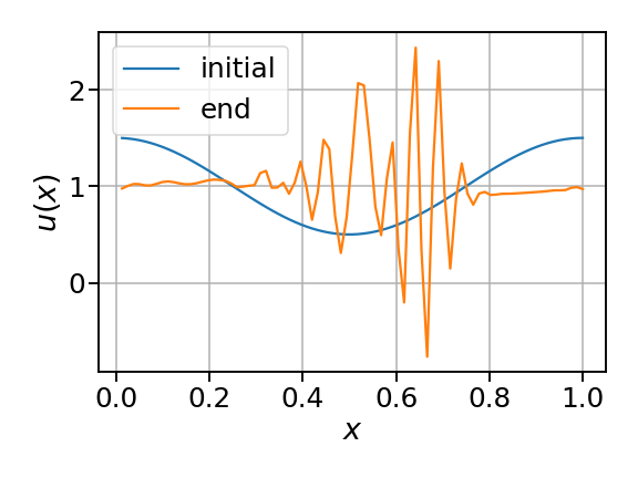
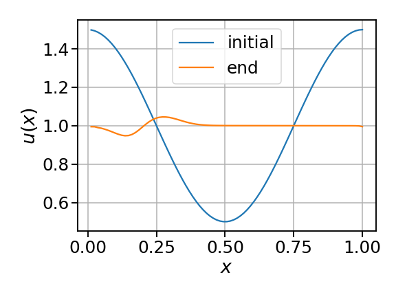
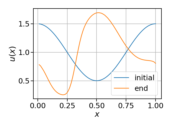
In the case of mildly stiff problems, $\delta=0.05$, the original MPRK [6] solution with $m=2$ in Fig. 2(a) is unstable because of problem stiffness, and the single-rate IMEX solution is unstable because the explicit part violates local CFL conditions (Fig. 2(b)). The multirate ($m=2$) explicit-implicit A-stable solution combines the stability features of both methods and is stable and efficient because of local time stepping on the explicit part and the implicit component (Fig. 2(c)). In Fig. 2(f) we show the solution in the same setting as shown in Fig. 2(b) except that the wave speed takes a 4:1 ratio between fast and slow (see Fig. 1) and we use an $m=4$, which means that the fast integrator takes four time steps with $\Delta t/4$ for each slow integrator step in the slow region.

For stiff problems, $\delta=100$, the A-stable method (§3.1) is not stable (see Fig. 2(d)); however, the L-stable method (§3.2) becomes stable (see Fig. 2(e)) at the cost of reducing the implicit accuracy order to one.

Mildly stiff $\rightarrow$ $\delta=.05$; mass loss: 2(a): 2.4e+50; 2(b): 0.0 ; 2(c): 1.1e-16

(a) explicit multirate (16)

(b) single-rate IMEX

(c) multirate w/ implicit (26)

Stiff $\rightarrow$ $\delta=100$; mass loss: (2(d): 4e-13; 2(e): 6e-13; 2(f): 7.8-16

(d) A-stable multirate (26)

(e) L-stable multirate (35)

(f) 2(c) with $m=4$

Figure 2: Results integrating (36) by using a finite volume method in space and various time integrators with $\Delta x=0.012$ ($M=81$ grid points), fixed $\Delta t=0.0125$ (CFL=$\omega(x)$), and final time $t_{F}=0.3$. The resulting advective CFL is 1.92 on the fast region and 1.01 on the slow region. The discrete mass loss is defined as $\Delta x\left\|\sum_{k=1}^{M}u_{k}(t_{0})-\sum_{k=1}^{M}u_{k}(t_{F})\right\|$.

5 Conclusions

We propose a new conservative method that extends an explicit multirate method to A- and L-stable implicit multirate-explicit methods. These extensions are first and second order and can accommodate telescopic multirate nesting. Therefore, these methods are suitable for AMR PDE discretizations with stiff terms that are being treated with a single-rate method. Such time-stepping schemes remove the stiffness stability limitation of existing conservative explicit multirate methods applied to adaptive mesh refinement PDE discretizations, thus allowing them to be applied to problems with stiff components as well. An advection diffusion problem is used to demonstrate the stability properties of the new methods.

References

- Mittal et al. [2021] Ketan Mittal, Som Dutta, and Paul Fischer. Multirate timestepping for the incompressible Navier-Stokes equations in overlapping grids. Journal of Computational Physics, 437:110335, 2021.
- Roberts et al. [2021] Steven Roberts, John Loffeld, Arash Sarshar, Carol S Woodward, and Adrian Sandu. Implicit multirate GARK methods. Journal of Scientific Computing, 87(1):1–32, 2021.
- Grote et al. [2015] Marcus J Grote, Michaela Mehlin, and Teodora Mitkova. Runge–Kutta-based explicit local time-stepping methods for wave propagation. SIAM Journal on Scientific Computing, 37(2):A747–A775, 2015.
- Seny et al. [2013] Bruno Seny, Jonathan Lambrechts, Richard Comblen, Vincent Legat, and J-F Remacle. Multirate time stepping for accelerating explicit discontinuous Galerkin computations with application to geophysical flows. International Journal for Numerical Methods in Fluids, 71(1):41–64, 2013.
- Sandu [2019] Adrian Sandu. A class of multirate infinitesimal GARK methods. SIAM Journal on Numerical Analysis, 57(5):2300–2327, 2019.
- Constantinescu and Sandu [2007] Emil M. Constantinescu and Adrian Sandu. Multirate timestepping methods for hyperbolic conservation laws. Journal of Scientific Computing, 33(3):239–278, December 2007. doi: 10.1007/s10915-007-9151-y.
- Kang and Constantinescu [2021] Shinhoo Kang and Emil M. Constantinescu. Entropy-preserving and entropy-stable relaxation IMEX and multirate time-stepping methods. Submitted, 2021. URL https://arxiv.org/abs/2108.08908.
- Carciopolo et al. [2019] Ludovica Delpopolo Carciopolo, Luca Bonaventura, Anna Scotti, and Luca Formaggia. A conservative implicit multirate method for hyperbolic problems. Computational Geosciences, 23(4):647–664, 2019.
- Constantinescu and Sandu [2013] E.M. Constantinescu and A. Sandu. Extrapolated multirate methods for differential equations with multiple time scales. Journal of Scientific Computing, 56(1):28–44, 2013. doi: 10.1007/s10915-012-9662-z.
- Bonaventura et al. [2020] Luca Bonaventura, Francesco Casella, L Delpopolo Carciopolo, and Akshay Ranade. A self adjusting multirate algorithm for robust time discretization of partial differential equations. Computers & Mathematics with Applications, 79(7):2086–2098, 2020.
- Giraldo et al. [2013] F.X. Giraldo, J.F. Kelly, and E.M. Constantinescu. Implicit-explicit formulations of a three-dimensional nonhydrostatic unified model of the atmosphere (NUMA). SIAM Journal on Scientific Computing, 35(5):B1162–B1194, 2013. doi: 10.1137/120876034.