KEK-TH-2380

Backpropagating Hybrid Monte Carlo algorithm
for fast Lefschetz thimble calculations

Genki Fujisawa¹⁾, Jun Nishimura^1,2),

Katsuta Sakai²⁾ and Atis Yosprakob¹⁾

¹⁾Department of Particle and Nuclear Physics,
School of High Energy Accelerator Science,
Graduate University for Advanced Studies (SOKENDAI),
1-1 Oho, Tsukuba, Ibaraki 305-0801, Japan

²⁾KEK Theory Center, Institute of Particle and Nuclear Studies,
High Energy Accelerator Research Organization,
1-1 Oho, Tsukuba, Ibaraki 305-0801, Japan

The Picard-Lefschetz theory has been attracting much attention as a tool to evaluate a multi-variable integral with a complex weight, which appears in various important problems in theoretical physics. The idea is to deform the integration contour based on Cauchy’s theorem using the so-called gradient flow equation. In this paper, we propose a fast Hybrid Monte Carlo algorithm for evaluating the integral, where we “backpropagate” the force of the fictitious Hamilton dynamics on the deformed contour to that on the original contour, thereby reducing the required computational cost by a factor of the system size. Our algorithm can be readily extended to the case in which one integrates over the flow time in order to solve not only the sign problem but also the ergodicity problem that occurs when there are more than one thimbles contributing to the integral. This enables, in particular, efficient identification of all the dominant saddle points and the associated thimbles. We test our algorithm by calculating the real-time evolution of the wave function using the path integral formalism.

1 Introduction

Many problems in theoretical physics are formulated in terms of a multi-variable integral with some weight, where the number of variables or the system size is typically very large. If the weight is positive semi-definite, we can regard it as a probability distribution and perform Monte Carlo calculation based on the idea of importance sampling. However, it is not straightforward to extend this method to the case with a complex weight. For instance, if we use the absolute value of the complex weight as the probability distribution for sampling and take into account the phase factor by reweighting, huge cancellation occurs among the sampled configurations. For this reason, one needs exponentially large numbers of configurations as the system size increases in order to obtain results with sufficient precision. This is the sign problem, which has been hindering the development of theoretical physics in various branches.

The situation regarding the sign problem has changed drastically in the last decade, however. There is by now a bunch of new techniques that have proven to work beautifully in certain classes of problems. For instance, the tensor renormalization group [1, 2, 3, 4, 5] is applicable if one can reformulate the problem in terms of a network of tensors, where the indices of tensors are contracted with those of the adjacent tensors. This method does not rely on the importance sampling, and hence the sign problem is absent from the outset.

Another promising direction is to complexify the integration variables keeping the holomorphicity of the weight and the observables. There are roughly two methods that belong to this category. One of them is the complex Langevin method (CLM) [6, 7, 8, 9, 10, 11], which can be viewed as a naive extension of the ordinary Langevin method for positive semi-definite weights. In this method, the expectation values of observables can be obtained with configurations generated by solving the complex Langevin equation, which involves the Gaussian noise term and the drift term representing the derivative of the weight. The computational cost is comparable to that of ordinary Monte Carlo methods for positive semi-definite weights. The validity of this method requires, however, that the probability distribution of the drift term and that of the observables should fall off sufficiently fast at large values, which is not always satisfied [10, 11]. While the method is definitely worth trying for its simplicity and its capability for large system size (See, for instance, Refs. [12, 13, 14, 15, 16, 17] for semi-realistic calculations.), one needs to have the luck of satisfying the validity condition in order to explore the most interesting parameter regime.

The other method based on complexification of integration variables uses Cauchy’s theorem and deforms the integration contour in such a way that the integrand does not oscillate much in phase. One can then apply standard Monte Carlo methods to perform the integration along the deformed contour. The crucial question is how to find an optimal deformed contour. A rigorous answer to this question is provided by the Picard-Lefschetz theory. This theory asserts that an optimal deformed contour is given by a certain set of Lefschetz thimbles, which represent the steepest descent contours in the complexified configuration space originating from saddle points of the complex weight [21, 22, 23, 24]. This set of thimbles can be obtained by solving the gradient flow equation, which involves the gradient of the complex weight, starting from a point on the original contour [25].

In practical applications, it turns out beneficial to keep finite the “flow time”, the amount of the contour deformation by the flow equation, so that one obtains an integration contour which interpolates the original contour and the set of Lefschetz thimbles [25]. In particular, this avoids the ergodicity problem or the multi-modality problem that arises when there are more than one thimbles contributing to the integral, which are either disconnected or connected at a zero of the complex weight [26]. Furthermore, in order to solve the sign problem and the ergodicity problem at the same time, it has been proposed to perform sampling on the “worldvolume” [30], which consists of a one-parameter family of the integration contour obtained for various flow time. Including all these ideas, we use the word “the generalized (Lefschetz) thimble method” (GTM) (See Ref. [31] for a review.) to refer to the Monte Carlo method based on the Picard-Lefschetz theory.

While the GTM does not have the validity issue that exists in the CLM, its crucial disadvantage concerns the computational cost. Solving the gradient flow equation is similar in this respect to solving the complex Langevin equation. However, one still needs to search for the configurations on the deformed contour that make important contribution to the integral. If one uses the plain Metropolis algorithm to do this, one cannot move fast in the configuration space keeping the acceptance rate reasonably high, which necessarily limits the system size to be small.

In this paper, we propose a fast Hybrid Monte Carlo (HMC) algorithm that can be used in the GTM. In this algorithm, one updates the configuration by solving a fictitious Hamilton equation of motion using the gradient of the absolute value of the weight as the force so that one can move very efficiently in the configuration space. In fact, various HMC algorithms were proposed in the process of developing the GTM [24, 29, 30]. These algorithms solve the Hamilton equation of motion on the deformed contour [24, 29] or on the worldvolume [30], which we shall refer to as the deformed manifold collectively in what follows. This requires complicated procedures of determining a constrained motion on the deformed manifold, which is unknown a priori. In addition to the force obtained by taking the derivative of the modulus of the complex weight, one has the normal force characteristic to constrained systems, which has to be determined in such a way that the complexified configuration is constrained on the deformed manifold. This is done by Newton’s method, which requires solving the flow equation at each iteration.

Here we consider solving the Hamilton equation of motion on the original contour, which saves us from all the burden associated with treating the constrained motion. The main task is transferred to the calculation of the force, which requires differentiating the modulus of the complex weight evaluated on the deformed manifold, now with respect to the configuration on the original contour. At first sight, one might think that this requires the calculation of the Jacobian matrix associated with the deformation of the integration contour. The crucial point of our proposal is that one can actually avoid this calculation by “backpropagating” the force on the deformed contour to that on the original contour, which reduces the computational cost by a factor of the system size.

The only drawback of our HMC algorithm compared with the existing ones is that the modulus of the Jacobian is not included in sampling and hence should be taken into account by reweighting. Note, however, that the phase of the Jacobian has to be taken into account by reweighting anyway in the GTM in general. The calculation of the Jacobian is time-consuming, but it can be done off-line since it is needed only when one measures the observables for statistically decorrelated configurations obtained by the HMC algorithm. If one uses a crude estimator of the Jacobian [33], the computational cost of the GTM becomes comparable to ordinary Monte Carlo methods just like the CLM. Thus our algorithm opens up a new possibility for applying the GTM to large systems.

The rest of this paper is organized as follows. In Section 2, we briefly review the GTM. In Section 3, we present our HMC algorithm on the original contour. In Section 4, we extend our algorithm to the case in which one integrates over the flow time to avoid the ergodicity problem. In Section 5, we clarify the relationship to the existing HMC algorithms. In Section 6, we test our algorithm by calculating the real-time evolution of the wave function using the path integral formalism. Section 7 is devoted to a summary and discussions. In Appendix A, we provide a simple understanding for the reduction of computational cost by backpropagation. In Appendices B and C, we provide some notes related to Section 5.

2 Brief review of the GTM

In this section, we briefly review the GTM for a general model given by the partition function

$$Z=\int dx\,e^{-S(x)}\ ,$$ (2.1)

where the action $S(x)$ is a complex function of $x=(x_{1},\cdots,x_{N})\in\mathbb{R}^{N}$. The expectation value of an observable $\mathcal{O}(x)$ is defined by

$$\langle\mathcal{O}(x)\rangle=\frac{1}{Z}\int dx\,\mathcal{O}(x)\,e^{-S(x)}\ .$$ (2.2)

In the GTM [25], we deform the integration contour into $\mathbb{C}^{N}$ by using the so-called holomorphic gradient flow equation

$$\frac{\partial}{\partial\sigma}z_{k}(x,\sigma)=\overline{\frac{\partial S(z(x,\sigma))}{\partial z_{k}}}\ ,$$ (2.3)

which is solved from $\sigma=0$ to $\sigma=\tau$ with the initial condition $z(x,0)=x\in\mathbb{R}^{N}$. The flowed configurations define an $N$-dimensional real manifold embedded in $\mathbb{C}^{N}$, which we denote as $M_{\tau}=\{z(x,\tau)|x\in\mathbb{R}^{N}\}$. According to Cauchy’s theorem, the integration contour can be deformed continuously from $\mathbb{R}^{N}$ to $M_{\tau}\subset\mathbb{C}^{N}$ without changing the partition function. Then, by noting that $z=z(x,\tau)$ defines a one-to-one map from $x\in\mathbb{R}^{N}$ to $z\in M_{\tau}$, one can rewrite the partition function as

$$Z=\int_{M_{\tau}}dz\,e^{-S(z)}=\int dx\,e^{-S(z(x,\tau))}\,\mathrm{det}J(x,\tau)\ ,$$ (2.4)

and similarly the observable (2.2) as

$$\langle\mathcal{O}(x)\rangle=\frac{1}{Z}\int dx\,\mathcal{O}(z(x,\tau))e^{-S(z(x,\tau))}\,\mathrm{det}J(x,\tau)\ ,$$ (2.5)

where the Jacobian matrix $J(x,\tau)$ corresponding to the map $z(x,\tau)$ is defined by

$$J_{kl}(x,\sigma)\equiv\frac{\partial z_{k}(x,\sigma)}{\partial x_{l}}\ .$$ (2.6)

Taking the derivative with respect to $x_{l}$ on each side of (2.3), one obtains the differential equation for $J(x,\sigma)$ as

$$\frac{\partial}{\partial\sigma}J_{kl}(x,\sigma) =\overline{H_{km}(z(x,\sigma))}\,\overline{J_{ml}(x,\sigma)}\ ,$$ (2.7)

which can be solved from $\sigma=0$ to $\sigma=\tau$ with the initial condition $J_{kl}(x,0)=\delta_{kl}$ to obtain the Jacobian matrix $J(x,\tau)$. Here we have defined the Hessian of the action as

$$H_{ij}(z) =\frac{\partial^{2}S(z)}{\partial z_{i}\partial z_{j}}\ ,$$ (2.8)

which plays an important role in this paper. Note that the Hessian is a sparse matrix with only O($N$) nonzero elements if the action is local, meaning that only terms with local couplings among $z_{i}$’s exist as in the case of local field theories.

The virtue of using the holomorphic gradient flow (2.3) in deforming the integration contour can be understood by taking the derivative of the action with respect to the flow time as

$$\frac{\partial}{\partial\sigma}S(z(x,\sigma)) =\frac{\partial z_{k}(z(x,\sigma))}{\partial\sigma}\,\frac{\partial S(z(x,\sigma))}{\partial z_{k}}=\overline{\frac{\partial S(z(x,\sigma))}{\partial z_{k}}}\,\frac{\partial S(z(x,\sigma))}{\partial z_{k}}\geq 0\ ,$$ (2.9)

which implies that the real part of the action $S$ grows monotonically along the flow while keeping the imaginary part constant. Thus, in the $\sigma\rightarrow\infty$ limit, ${\rm Re}S(z(x,\sigma))$ diverges except for such points $x=x^{\star}$ that satisfy $\lim_{\sigma\rightarrow\infty}\frac{\partial}{\partial z_{k}}S(z(x^{\star},\sigma))=0$, which are the points that flow into some fixed points $z=z^{\star}$ defined by $\frac{\partial S(z^{\star})}{\partial z_{k}}=0$. The deformed contour $M_{\tau}$ at $\tau=\infty$ consists of a set of Lefschetz thimbles associated with these fixed points, which correspond to the infinitesimal vicinities of the points $x^{\star}$ on the original contour. Since $\mathrm{Im}S(z(x))$ is constant on each thimble, the sign problem is maximally reduced. The original proposal was to perform Monte Carlo integration on these thimbles [22, 23, 24].

However, when there are more than one thimbles, the transition between thimbles does not occur during the Monte Carlo simulation, which leads to the violation of ergodicity. The GTM [25] avoids this problem by choosing a sufficiently small flow time allowing the $\mathrm{Im}S(z(x))$ to fluctuate to some extent, which works as far as the system size is not so large. For a larger system size, one can integrate over the flow time in order to avoid the sign problem and the ergodicity problem at the same time [30].

3 HMC algorithm with backpropagation

In this section, we discuss our HMC algorithm on the original contour. The crucial point is to calculate the force in the fictitious Hamilton dynamics by using the idea of backpropagation, which reduces the computational cost by a factor of O($N$). Here we consider the case of fixed $\tau$ and defer the discussion in the case of integrating $\tau$ to Section 4.

3.1 HMC algorithm on the original contour

In order to simulate the partition function (2.4), let us consider the partition function

$$Z_{\tau}=\int_{\mathbb{R}^{N}}dx\,e^{-{\rm Re}S(z(x,\tau))}\ ,$$ (3.1)

where the imaginary part of the action $S$ as well as the Jacobian is omitted. The expectation value (2.5) can be obtained by the standard reweighting formula as

$$\langle\mathcal{O}(x)\rangle=\frac{\langle\mathcal{O}(z(x,\tau))e^{-i\mathrm{Im}S(z(x,\tau))}\mathrm{det}J(x,\tau)\rangle_{\tau}}{\langle e^{-i\mathrm{Im}S(z(x,\tau))}\mathrm{det}J(x,\tau)\rangle_{\tau}}\ ,$$ (3.2)

where $\langle\cdots\rangle_{\tau}$ represents the expectation value with respect to the partition function (3.1).

The most naive way to simulate the partition function (3.1) is the Metropolis algorithm. Starting from some configuration $x\in\mathbb{R}^{N}$, one constructs a trial configuration $x^{\prime}=x+\delta x\in\mathbb{R}^{N}$ with certain probability distribution for $\delta x$. Then one calculates the change of the action

$$\delta S=\mathrm{Re}S(z(x^{\prime},\tau))-\mathrm{Re}S(z(x,\tau))\ ,$$ (3.3)

and accepts the trial configuration with the probability $\min(1,e^{-\delta S})$. Both the numerator and the denominator in (3.2) can be obtained by taking an average over the configurations generated by the above algorithm. While this algorithm is very easy to implement, it is not efficient since the update by $\delta x$ has to be local in order to keep the acceptance rate reasonably high.

The basic idea of the HMC algorithm [34] is to enable a global update $\delta x$ in the Metropolis algorithm by using the information of the action in its proposal. For that, we introduce auxiliary variables $p_{i}$ corresponding to $x_{i}$ and consider the partition function

$$\tilde{Z}_{\tau} =\int dx\,dp\,e^{-H}\ ,$$ (3.4)

$$H =\frac{1}{2}(p_{i})^{2}+{\rm Re}S(z(x,\tau))\ ,$$ (3.5)

which is equivalent to (3.1). One can update $p_{i}$ by just generating Gaussian random numbers. After that, using the initial condition for $x(0)$ and $p(0)$ set by the current configuration, one solves the fictitious Hamilton equation

$$\frac{dx_{i}(s)}{ds} =p_{i}(s)\ ,$$

$$\frac{dp_{i}(s)}{ds} =F_{i}(s)\ ,$$ (3.6)

where the force $F_{i}(s)$ is defined by

$$F_{i}(s) =-\left.\frac{\partial{\rm Re}S(z(x,\tau))}{\partial x_{i}}\right|_{x=x(s)}$$ (3.7)

for a fixed time $s_{\rm f}$ to obtain $x(s_{\rm f})$ and $p(s_{\rm f})$, which provide the trial configuration subject to the Metropolis accept/reject procedure with the probability $\min(1,e^{-\delta H})$, where

$$\delta H =H(x(s_{\rm f}),p(s_{\rm f}))-H(x(0),p(0))\ .$$ (3.8)

If one can solve (3.6) exactly, one obtains $\delta H=0$ due to the Hamiltonian conservation, which implies that the acceptance rate is 100%. In practice, one has to discretize the Hamilton equation, which makes $\delta H\neq 0$. The stepsize $\Delta s$ has to be chosen small enough to keep the acceptance rate reasonably high. Note that the detailed balance is satisfied even at finite $\Delta s$ thanks to the Metropolis procedure, and hence there is no systematic error due to the discretization of the Hamilton equation. See Section 6.2 for more detail.

3.2 Calculating the force by backpropagation

Thus the question boils down to the calculation of (3.7). Let us first note that (3.7) can be rewritten as

$$F_{j}(s) =2\,{\rm Re}\left\{f_{i}J_{ij}(x(s),\tau)\right\}\ ,$$ (3.9)

where $J_{ij}(x,\tau)$ is the Jacobian matrix defined by (2.6) and $f_{i}(s)$ is the gradient of the action on the deformed contour

$$f_{i} =-\left.\frac{\partial{\rm Re}S(z)}{\partial z_{i}}\right|_{z=z(x(s),\tau)}$$ (3.10)

at $z(x(s),\tau)$ corresponding to the point $x(s)$ on the original contour. The calculation of the Jacobian matrix, however, requires us to solve the differential equation (2.7), which involves O($N^{2}$) or O($N^{3}$) arithmetic operations depending on whether the action $S(z)$ is local or non-local in the sense explained below (2.8). Alternatively, one might think of evaluating the right-hand side of (3.7) by numerical derivative as in Ref. [32]. The required cost, however, is comparable to calculating the Jacobian, and what is worse, there is some systematic error associated with the numerical derivative.

Suppose we were to calculate $J_{ij}(x,\tau)\,v_{j}$ with $v_{j}\in{\mathbb{R}}$, which appears many times in the HMC algorithm on the deformed manifold [29, 30]. In this case, one can avoid the calculation of $J_{ij}(x,\tau)$ itself by noticing that $v_{i}(\sigma)\equiv J_{ij}(x,\sigma)\,v_{j}$ satisfies the flow equation

$$\frac{\partial}{\partial\sigma}v_{i}(\sigma)=\overline{H_{ij}(z(x,\sigma))}\,\overline{v_{j}(\sigma)}\ .$$ (3.11)

Solving this from $\sigma=0$ to $\sigma=\tau$ with the initial condition $v_{i}(0)=v_{i}$ requires O($N$) or O($N^{2}$) arithmetic operations depending on whether the action $S(z)$ is local or non-local. Thus one can save a factor of O($N$).

Coming back to our problem, we can actually save a factor of O($N$) as well but in a slightly different way. Let us note that the problem of calculating (3.7) is mathematically equivalent to the calculation in machine learning, where ${\rm Re}S(z(x,\tau))$ represents the loss function and $z_{i}(x,\tau)$ represents the parameters of the network at a layer labeled with $\tau$. The quantity (3.7) we have to calculate is the derivative of the loss function with respect to $x_{i}=z_{i}(x,0)$, which represent the parameters at the first layer. The crucial idea here is the use of backpropagation. Let us define the “force” at flow time $\sigma$ by

$$f_{i}(\sigma) =-\frac{\partial{\rm Re}S(z(x,\tau))}{\partial z_{i}(x,\sigma)}\ .$$ (3.12)

Applying the chain rule, we obtain

$$f_{j}(\sigma-\varepsilon) =f_{i}(\sigma)\frac{\partial z_{i}(x,\sigma)}{\partial z_{j}(x,\sigma-\varepsilon)}+\overline{f_{i}(\sigma)}\frac{\partial\overline{z_{i}(x,\sigma)}}{\partial z_{j}(x,\sigma-\varepsilon)}$$ (3.13)

$$\sim f_{j}(\sigma)+\varepsilon\,\overline{f_{i}(\sigma)}\,H_{ij}(\sigma)\ .$$ (3.14)

This implies that $f_{i}(\sigma)$ obeys the differential equation

$$\frac{d}{d\sigma}f_{j}(\sigma) =-\overline{f_{i}(\sigma)}\,H_{ij}(\sigma)\ ,$$ (3.15)

which is analogous to (3.11). By solving this differential equation backwards in $\sigma$ from $\sigma=\tau$ to $\sigma=0$ with the initial condition $f_{i}(\tau)=f_{i}$, one obtains the force at the first layer

$$f_{i}(0) =-\frac{\partial{\rm Re}S(z(x,\tau))}{\partial z_{i}(x,0)}\ .$$ (3.16)

Using this, the desired force (3.7) is obtained as

$$F_{i} =-\frac{\partial{\rm Re}S(z(x,\tau))}{\partial z_{i}(x,0)}-\frac{\partial{\rm Re}S(z(x,\tau))}{\partial\bar{z}_{i}(x,0)}=2\,{\rm Re}f_{i}(0)\ .$$ (3.17)

Thus the computational cost is reduced by a factor of O($N$).

3.3 Discretizing the flow equation

In actual calculations, one has to discretize the holomorphic gradient flow equation (2.3). In this section, we explain how our idea for calculating the force in the fictitious Hamilton dynamics can be extended to this case. In particular, we show that this can be done in such a way that the discretization causes neither systematic errors nor any decrease in the acceptance rate, which is not the case for the existing HMC algorithms [29, 30] as we discuss in Section 5.

Let us define $\sigma_{n}=n\,\varepsilon$ ($n=0,1,\cdots,N_{\tau}$) with $\tau=N_{\tau}\,\varepsilon$ and consider the holomorphic gradient flow (2.3) discretized as

$$z_{k}(x,\sigma_{n+1})=z_{k}(x,\sigma_{n})+\varepsilon\,\overline{\frac{\partial S(z(x,\sigma_{n}))}{\partial z_{k}}}$$ (3.18)

with the initial condition $z(x,0)=x\in\mathbb{R}^{N}$. Taking the derivative with respect to $x_{l}$ on each side of (3.18), one obtains

$$J_{kl}(x,\sigma_{n+1})=J_{kl}(x,\sigma_{n})+\varepsilon\,\overline{H_{km}(z(x,\sigma_{n}))}\,\overline{J_{ml}(x,\sigma_{n})}\ .$$ (3.19)

By solving this difference equation with the initial condition $J_{kl}(x,0)=\delta_{kl}$, one obtains exactly the Jacobian matrix (2.6) defined for the solution to the discretized flow equation (3.18). This means that while finite $\varepsilon$ affects the deformed contour, thanks to Cauchy’s theorem, it does not affect the equations (2.4) and (2.5), and hence does not cause any systematic error.

Let us then discuss how the calculation of the force (3.7) should be extended to the case of the discretized flow equation. If one uses (3.9), the Jacobian matrix has to be obtained by solving (3.19), which is time consuming. Instead, we define the “force” at flow time $\sigma_{n}$ by

$$f_{i}(\sigma_{n}) =-\frac{\partial{\rm Re}S(z(x,\tau))}{\partial z_{i}(x,\sigma_{n})}\ .$$ (3.20)

Applying the chain rule, we obtain

$$f_{j}(\sigma_{n-1}) =f_{i}(\sigma_{n})\frac{\partial z_{i}(x,\sigma_{n})}{\partial z_{j}(x,\sigma_{n-1})}+\overline{f_{i}(\sigma_{n})}\frac{\partial\overline{z_{i}(x,\sigma_{n})}}{\partial z_{j}(x,\sigma_{n-1})}$$ (3.21)

$$=f_{j}(\sigma_{n})+\varepsilon\,\overline{f_{i}(\sigma_{n})}H_{ij}(\sigma_{n-1})\ .$$ (3.22)

By solving this difference equation backwards in $\sigma$ from $\sigma=\tau$ to $\sigma=0$ with the initial condition $f_{i}(\tau)=f_{i}$, one obtains the force at the first layer (3.16). Using this, the desired force is obtained as (3.17). The computational cost is reduced by a factor of O($N$) similarly to the case of the continuous flow equation. In Appendix A, we provide a simple understanding for this huge reduction of computational cost.

4 Integrating over the flow time $\tau$

In order to solve the sign problem, the flow time $\tau$ has to be sufficiently large. However, when one has more than one Lefschetz thimbles at $\tau=\infty$, Monte Carlo simulations based on the HMC algorithm suffer from the ergodicity problem. This occurs because the regions that contribute to the integral are either disconnected or separated by singular points, at which the real part of the action diverges. In order to solve the sign problem without suffering from this ergodicity problem, it is useful to integrate over the flow time. This is the idea of the “worldvolume approach” [30], which was put forward in the context of the HMC algorithm on the deformed contour. Here we adapt this idea to our HMC algorithm on the original contour, which not only turns out to be much simpler but also solves a possible problem in the original proposal.

4.1 The basic idea

The key observation here is that in the reweighting formula (3.2), the ratio is $\tau$-independent although both the numerator and the denominator on the right-hand side depend on $\tau$. This implies that one can actually integrate over $\tau$ and consider

$$Z_{W}=\int d\tau\,e^{-W(\tau)}\int dx\,e^{-{\rm Re}S(z(x,\tau))}\ ,$$ (4.1)

where $W(\tau)$ is a real function of $\tau$ that can be chosen so that the distribution of $\tau$ becomes almost uniform within a certain range [30]. The expectation value of an observable can be calculated as

$$\langle\mathcal{O}(x)\rangle=\frac{\langle\mathcal{O}(z(x,\tau))e^{-i\mathrm{Im}S(z(x,\tau))}\mathrm{det}J(x,\tau)e^{-\widetilde{W}(\tau)}\rangle_{W}}{\langle e^{-i\mathrm{Im}S(z(x,\tau))}\mathrm{det}J(x,\tau)e^{-\widetilde{W}(\tau)}\rangle_{W}}\ ,$$ (4.2)

where $\langle\cdots\rangle_{W}$ represents the expectation value with respect to the partition function (4.1). We have introduced an arbitrary function $\widetilde{W}(\tau)$, which can be chosen to minimize the statistical errors [36].

4.2 Extending our HMC algorithm

Let us extend our HMC algorithm to the model (4.1). As we did in the previous section, we introduce auxiliary variables $(p_{i},p_{\tau})$ corresponding to $(x_{i},\tau)$ and consider the partition function

$$\tilde{Z}_{W} =\int d\tau\,dp_{\tau}\,dx\,dp\,e^{-H}\ ,$$ (4.3)

$$H =\frac{1}{2}(p_{i})^{2}+\frac{1}{2}(p_{\tau})^{2}+{\rm Re}S(z(x,\tau))+W(\tau)\ .$$ (4.4)

The Hamilton equation for $x_{i}(s)$ and $p_{i}(s)$ are given by (3.6) as before, but here we also have the equations for $\tau(s)$ and $p_{\tau}(s)$ given by

$$\frac{d\tau(s)}{ds} =p_{\tau}(s)\ ,$$ (4.5)

$$\frac{dp_{\tau}(s)}{ds} =-\left.\frac{dW(\tau)}{d\tau}\right|_{\tau=\tau(s)}+F_{\tau}(s)\ ,$$ (4.6)

where the force $F_{\tau}(s)$ for $\tau$ is defined by

$$F_{\tau}(s) =-\left.\frac{\partial{\rm Re}S(z(x,\tau))}{\partial\tau}\right|_{x=x(s),\tau=\tau(s)}\ .$$ (4.7)

Using the flow equation (2.3), one can rewrite it as

$$F_{\tau}(s) =-\left|\left.\frac{\partial S(z)}{\partial z_{i}}\right|_{z=z(x(s),\tau(s))}\right|^{2}\ .$$ (4.8)

4.3 Discretizing the flow equation keeping $\tau$ continuous

In actual calculations, we have to discretize the flow equation by $\tau=N_{\tau}\,\varepsilon$. The integration over $\tau$ should then be replaced by the integration over the flow stepsize $\varepsilon$, and the Hamilton equation (4.5), (4.6) should be regarded as describing the fictitious time evolution of the flow stepsize $\varepsilon$.

The calculation of the force (4.7) in the $\tau$-direction requires some care. Note that (4.8) is obtained by using the continuum version of the flow equation (2.3). Therefore, if one uses (4.8) naively, the Hamiltonian conservation in the HMC algorithm is violated by the discretization of the flow equation. Instead, we have to calculate (4.7) as

$$F_{\tau}(s) =-\frac{1}{N_{\tau}}\left.\frac{\partial{\rm Re}S(z(x,N_{\tau}\varepsilon))}{\partial\varepsilon}\right|_{x=x(s),\tau=\tau(s)}$$ (4.9)

$$=-\frac{1}{N_{\tau}}{\rm Re}\left\{\left.\frac{\partial z_{k}(x,N_{\tau}\varepsilon)}{\partial\varepsilon}\right|_{x=x(s),\,\varepsilon=\tau(s)/N_{\tau}}\left.\frac{\partial S(z(x,\tau))}{\partial z_{k}}\right|_{x=x(s),\tau=\tau(s)}\right\}\ ,$$ (4.10)

where $z_{k}(x,N_{\tau}\varepsilon)$ is obtained by solving the difference equation (3.18). Taking the $\varepsilon$-derivative on each side of (3.18), where $\sigma_{n}(\varepsilon)=n\,\varepsilon$ is treated now as a function of $\varepsilon$, we obtain

$$\frac{\partial z_{k}(x,\sigma_{n+1})}{\partial\varepsilon}=\frac{\partial z_{k}(x,\sigma_{n})}{\partial\varepsilon}+\varepsilon\,\overline{H_{kj}(\sigma_{n})}\,\overline{\frac{\partial z_{j}(x,\sigma_{n})}{\partial\varepsilon}}+\overline{\frac{\partial S(z(x,\sigma_{n}))}{\partial z_{k}}}\ .$$ (4.11)

Solving this difference equation with the initial condition

$$\frac{\partial z_{j}(x,0)}{\partial\varepsilon}=0\ ,$$ (4.12)

one can obtain the first factor in (4.10). The computational cost for this procedure is comparable to that for calculating the force in the $x$-direction.

Note that this is an exact calculation of the force for finite $\varepsilon$, and hence there is no systematic error here, either. This is a significant advantage of our algorithm over the existing ones, in which the discretization of the flow equation causes some systematic error as we discuss below.

5 Relationship to the existing HMC algorithms

As we mentioned in the Introduction, there are HMC algorithms proposed for the GTM in the past. The difference from our HMC algorithm is that the existing ones [29, 30] deal with the Hamilton dynamics of the point $z(x,\tau)$ after the flow, whereas we deal with the Hamilton dynamics of the point $(x,\tau)$ before the flow. Since the two points are in one-to-one correspondence, we should be able to compare the Hamilton dynamics. In this section, we clarify the relationship between the two types of algorithms from this point of view. Some basic properties of the deformed manifold necessary to understand this section are recapitulated in Appendix B for the readers’ convenience.

Here we will discuss the case of integrating $\tau$. For that, in this Section alone, we introduce the notation $x_{\mu}$ and $p_{\mu}$ ($\mu=0,1,\cdots,N$) for the dynamical variables and the corresponding momenta, where we have defined $x_{0}\equiv\tau$ and $p_{0}\equiv p_{\tau}$. Accordingly, we will also use $z_{i}(x)$ instead of $z_{i}(x,\tau)$ for the flowed configuration. The flow equation can be assumed to be either discretized or continuous, which does not matter in our discussion below. The above notations enable us to obtain the results for the case of a fixed flow time $\tau$ by simply replacing the index $\mu=0,\cdots,N$ by $i=1,\cdots,N$.

The Hamilton dynamics of the point $z_{i}(x)$ is described by the Hamiltonian

$$H=\bar{\pi}_{i}\pi_{i}+V(z,\bar{z})\ ,$$ (5.1)

where $\pi_{i}$ is the momentum on the deformed manifold. Therefore, the Hamilton equation on the deformed manifold is given by

$$\frac{dz_{i}}{ds} =\pi_{i}\ ,$$ (5.2)

$$\frac{d\pi_{i}}{ds} =-\frac{\partial V(z,\bar{z})}{\partial\bar{z}_{i}}+{\cal N}_{i}\ ,$$ (5.3)

where ${\cal N}_{i}$ is the normal force, which is perpendicular to the tangent space of the deformed manifold, and hence does not affect the Hamiltonian conservation. The normal force ${\cal N}_{i}$ is determined in such a way that the momentum $\pi_{i}(s)$ resides in the tangent space of the deformed manifold at the point $z_{i}(s)$, which is constrained to be on the deformed manifold.

In fact, the Hamilton dynamics on the deformed manifold given above is not equivalent to the Hamilton dynamics on the original contour that we have considered. Instead, it is described by the Hamiltonian on the original contour that takes the form

$$H=\frac{1}{2}\,p_{\mu}K_{\mu\nu}(x)\,p_{\nu}+V(z(x),\bar{z}(x))\ ,$$ (5.4)

which involves a nontrivial kernel $K_{\mu\nu}(x)=K_{\nu\mu}(x)$ in the kinetic term to be specified later. The Hamilton equation therefore takes the form

$$\frac{dx_{\mu}}{ds} =K_{\mu\nu}(x)\,p_{\nu}\ ,$$ (5.5)

$$\frac{dp_{\mu}}{ds} =-\frac{\partial V(z(x),\bar{z}(x))}{\partial x_{\mu}}-\frac{1}{2}\,p_{\nu}\frac{\partial K_{\nu\lambda}(x)}{\partial x_{\mu}}p_{\lambda}\ .$$ (5.6)

The $s$-evolution of the flowed configuration $z_{i}(x(s))$ is then given by

$$\frac{dz_{i}}{ds} =\frac{\partial z_{i}}{\partial x_{\mu}}\,\frac{dx_{\mu}}{ds}=\frac{\partial z_{i}}{\partial x_{\mu}}K_{\mu\nu}(x)\,p_{\nu}\ .$$ (5.7)

Comparing this with (5.2), we obtain the relationship

$$\pi_{i}=\frac{\partial z_{i}}{\partial x_{\mu}}K_{\mu\nu}(x)\,p_{\nu}\ ,$$ (5.8)

which shows that the momentum $\pi_{i}$ on the deformed manifold resides in the tangent space as it should. Plugging (5.8) and $z_{i}=z_{i}(x)$ into (5.1), one obtains

$$H =p_{\mu}\,K_{\mu\lambda}(x)\,g_{\lambda\rho}(x)\,K_{\rho\nu}(x)\,p_{\nu}+V(z(x),\bar{z}(x))\ ,$$ (5.9)

where we have defined

$$g_{\lambda\rho}(x) ={\rm Re}\left(\overline{\frac{\partial z_{i}}{\partial x_{\lambda}}}\,\frac{\partial z_{i}}{\partial x_{\rho}}\right)\ .$$ (5.10)

Since (5.9) should be identified with (5.4), we obtain an identity $\frac{1}{2}\,K(x)=K(x)\,g(x)\,K(x)$, which implies

$$K(x)=\frac{1}{2}\,g^{-1}(x)\ .$$ (5.11)

Next, let us consider the $s$-evolution of the momentum $\pi_{i}(x)$ on the deformed manifold. From (5.8), we find

$$\frac{\partial\pi_{i}}{\partial s}= \frac{\partial z_{i}}{\partial x_{\mu}}K_{\mu\nu}(x)\,\frac{\partial p_{\nu}}{\partial s}+\frac{\partial x_{\lambda}}{\partial s}\frac{\partial}{\partial x_{\lambda}}\left(\frac{\partial z_{i}}{\partial x_{\mu}}K_{\mu\nu}(x)\right)\,p_{\nu}={\cal F}_{i}+{\cal N}_{i}^{\prime}\ ,$$ (5.12)

where we have defined

$${\cal F}_{i} =-\frac{\partial z_{i}}{\partial x_{\mu}}K_{\mu\nu}(x)\,\frac{\partial V(z(x),\bar{z}(x))}{\partial x_{\nu}}\ ,$$ (5.13)

$${\cal N}_{i}^{\prime} =-\frac{1}{2}\,\frac{\partial z_{i}}{\partial x_{\mu}}K_{\mu\nu}(x)\,p_{\lambda}\frac{\partial K_{\lambda\rho}(x)}{\partial x_{\nu}}p_{\rho}+K_{\nu\lambda}(x)\,p_{\lambda}\frac{\partial}{\partial x_{\nu}}\left(\frac{\partial z_{i}}{\partial x_{\mu}}K_{\mu\rho}(x)\right)\,p_{\rho}\ .$$ (5.14)

The first term ${\cal F}_{i}$ in (5.12) is given by

$${\cal F}_{i} =-\frac{\partial z_{i}}{\partial x_{\mu}}K_{\mu\nu}(x)\,\left(\frac{\partial z_{j}}{\partial x_{\nu}}\frac{\partial V(z,\bar{z})}{\partial z_{j}}+\frac{\partial\bar{z}_{j}}{\partial x_{\nu}}\frac{\partial V(z,\bar{z})}{\partial\bar{z}_{j}}\right)$$ (5.15)

$$=-\frac{\partial z_{i}}{\partial x_{\mu}}\{g^{-1}(x)\}_{\mu\nu}\,{\rm Re}\left(\overline{\frac{\partial z_{j}}{\partial x_{\nu}}}\,\frac{\partial V(z,\bar{z})}{\partial\bar{z}_{j}}\right)\ .$$ (5.16)

This is nothing but the gradient force $-\frac{\partial V(z,\bar{z})}{\partial\bar{z}_{i}}$ projected onto the tangent space. The second term ${\cal N}_{i}^{\prime}$ in (5.12) can be interpreted as the normal force that is needed to realize the constrained motion. This can be checked by confirming that its projection onto the tangent space vanishes identically; namely,

$${\rm Re}\left(\overline{\frac{\partial z_{i}}{\partial x_{\alpha}}}\,{\cal N}_{i}^{\prime}\right)=0\quad\quad\mbox{for all $\alpha$}\ .$$ (5.17)

See Appendix B for the details.

The appearance of the kernel $K=\frac{1}{2}\,g^{-1}$ in (5.4) can be understood also from the viewpoint of what we are simulating. The Hamilton dynamics we consider in Section 4.2 is intended to reproduce the partition function (4.1). This can be seen by integrating out the momentum variables in (4.3), which yields (4.1). If we have a nontrivial kernel $K=\frac{1}{2}\,g^{-1}$ as in (5.4), the integration over the momentum $p_{\mu}$ in (5.4) yields an extra factor $\sqrt{\det g(x)}$ in the partition function. This is nothing but the volume element of the deformed manifold since $g(x)$ defined by (5.10) represents the induced metric on the deformed manifold, which is embedded in ${\mathbb{C}}^{N}$. Thus our result (5.4) is consistent with the fact that the HMC algorithm using the Hamilton dynamics on the deformed manifold includes the volume element of the deformed manifold in the partition function [29, 30].

In the case of fixed $\tau$, the induced metric (5.10) is given by $g_{kl}={\rm Re}(J^{\dagger}J)_{kl}$ for the discretized flow equation. In the continuum limit $\varepsilon\rightarrow 0$ of the flow equation, we have ${\rm Im}(J^{\dagger}J)=0$, which implies that $\sqrt{\det g(x)}=|\det J(x)|$. (See Appendix C for the details.) Thus, neglecting the finite $\varepsilon$ effects, the modulus of the Jacobian is included in sampling, which may have certain advantage, but the price one has to pay seems overwhelming.

In the case of integrating $\tau$, on the other hand, one obtains $\sqrt{\det g(x)}=C(x)\,|\det J(x)|$ neglecting the finite $\varepsilon$ effects, where $C(x)\geq 0$ needs to be calculated and taken into account in reweighting [30]. Moreover, if the fixed point of the flow equation that contributes to the integral resides on the original contour, the volume element $\sqrt{\det g(x)}$ of the worldvolume vanishes at that point, which causes an ergodicity problem. In fact, this problem occurs because the induced metric $g_{\mu\nu}(x)$ on the worldvolume becomes singular at that point. Obviously, our HMC algorithm based on the Hamilton dynamics on the original contour is totally free from such problems.

Note also that the HMC algorithms on the deformed manifold in Refs.[29, 30] assume ${\rm Im}(J^{\dagger}J)=0$, which is violated upon discretization of the flow equation as we show in Appendix C. There are actually two places in which this assumption is used. One of them is, as already mentioned above, in the statement that the HMC algorithm on the deformed contour includes $|\det J|$ in sampling. The other is in constructing the basis vectors of ${\mathbb{C}}^{N}$ orthogonal to the tangent space, which are used in solving the constrained motion on the deformed manifold. Therefore, the HMC algorithms in Refs.[29, 30] suffer from systematic errors due to discretization of the flow equation. In contrast, nowhere in our HMC algorithm on the original contour have we used ${\rm Im}(J^{\dagger}J)=0$. Hence, our algorithm is free from systematic errors whatsoever.

6 Practical applications

In this section, we consider an important improvement of our algorithm suggested also from our discussion in Section 5. This makes the discretization of the Hamilton equation slightly more nontrivial as we describe below. We test our algorithm by applying it to the time evolution of the wave function in the path integral formalism.

6.1 Introducing a mass parameter in the HMC

As we have seen in Section 5, the Hamilton dynamics on the deformed manifold is equivalent to introducing a nontrivial kernel $K(x)=\frac{1}{2}g^{-1}(x)$ in (5.4) in the Hamilton dynamics on the original contour. In a similar spirit, for practical applications, we find it very important to generalize our HMC algorithm by introducing a $\tau$-dependent mass parameter $m(\tau)$ as

$$\tilde{Z}_{W} =\int d\tau\,dp_{\tau}\,dx\,dp\,e^{-H}\ ,$$ (6.1)

$$H =\frac{1}{2m(\tau)}(p_{i})^{2}+\frac{1}{2}(p_{\tau})^{2}+{\rm Re}S(z(x,\tau))+W(\tau)\ .$$ (6.2)

Note first that integration over the momentum gives a factor $m(\tau)^{N/2}$ in the partition function. In the case of fixed $\tau$, this is just a constant factor, while in the case of integrating $\tau$, it can be absorbed into the definition of $W(\tau)$ in (4.1). This also suggests that $m(\tau)$ should be chosen to be proportional to the typical value of $|\det J(x,\tau)|^{2/N}$ for various $x$ with fixed $\tau$.

The need for this improvement can be understood from the fact that the flow equation typically maps a small region on the original contour to an exponentially large region on the deformed contour at large $\tau$, where the scale factor is given by $|\det J(x,\tau)|^{1/N}$. Introducing the mass in the HMC changes the effective stepsize in solving the Hamilton equation on the original contour by the factor of $1/\sqrt{m(\tau)}$. Therefore, the above choice of $m(\tau)$ enables a random walk on the deformed manifold with almost uniform discretization.

From the Hamiltonian (6.2), the Hamilton equation is obtained as

$$\frac{dx_{i}(s)}{ds} =\frac{1}{m(\tau)}\,p_{i}(s)\ ,$$ (6.3)

$$\frac{dp_{i}(s)}{ds} =F_{i}(s)\ ,$$ (6.4)

$$\frac{d\tau(s)}{ds} =p_{\tau}(s)\ ,$$ (6.5)

$$\frac{dp_{\tau}(s)}{ds} =-\left.\frac{dW(\tau)}{d\tau}\right|_{\tau=\tau(s)}+F_{\tau}(s)+\frac{1}{2m(\tau)^{2}}\frac{dm(\tau)}{d\tau}(p_{i})^{2}\ ,$$ (6.6)

where the forces $F_{i}(s)$ and $F_{\tau}(s)$ are defined by (3.7) and (4.7), respectively, as before.

6.2 Discretizing the Hamilton equation in the HMC

In actual calculations, the Hamilton equation in the HMC algorithm has to be discretized. In the case of fixed $\tau$, the Hamiltonian takes the canonical form $H=\frac{1}{2}p^{2}+V(x)$ so that one can use the standard leap-frog discretization. This respects the reversibility and the preservation of the phase space volume [34], which guarantees the detailed balance. In the case of integrating $\tau$, one should note that the first term of the Hamiltonian (6.2) mixes the momentum variables $p_{i}$ with $\tau$, which is now treated as one of the coordinate variables. For this reason, we have to generalize the leap-frog discretization slightly.

Let us note first that the Hamilton equation takes the form

$$\frac{dp_{\tau}}{ds}=A(x,\tau,p)\ ,\quad\frac{dx}{ds}=B(\tau,p)\ ,\quad\frac{d\tau}{ds}=C(p_{\tau})\ ,\quad\frac{dp}{ds}=D(x,\tau)\ .$$ (6.7)

We discretize this equation as

$$p_{\tau}(s_{n+1/2}) =p_{\tau}(s_{n})+\frac{\Delta s}{2}\,A(x(s_{n}),\tau(s_{n}),p(s_{n}))\ ,$$ (6.8)

$$x(s_{n+1/2}) =x(s_{n})+\frac{\Delta s}{2}\,B(\tau(s_{n}),p(s_{n}))\ ,$$ (6.9)

$$\tau(s_{n+1/2}) =\tau(s_{n})+\frac{\Delta s}{2}\,C(p_{\tau}(s_{n+1/2}))\ ,$$ (6.10)

$$p(s_{n+1}) =p(s_{n})+\Delta s\,D(x(s_{n+1/2}),\tau(s_{n+1/2}))\ ,$$ (6.11)

$$\tau(s_{n+1}) =\tau(s_{n+1/2})+\frac{\Delta s}{2}\,C(p_{\tau}(s_{n+1/2}))\ ,$$ (6.12)

$$x(s_{n+1}) =x(s_{n+1/2})+\frac{\Delta s}{2}\,B(\tau(s_{n+1}),p(s_{n+1}))\ ,$$ (6.13)

$$p_{\tau}(s_{n+1}) =p_{\tau}(s_{n+1/2})+\frac{\Delta s}{2}\,A(x(s_{n+1}),\tau(s_{n+1}),p(s_{n+1}))\ ,$$ (6.14)

where $s_{\nu}=\nu\Delta s$ with $\nu$ being an integer or a half integer. We repeat the above procedure for $n=0,1,\cdots,(N_{s}-1)$, where $s_{\rm f}=N_{s}\Delta s$ represents the total fictitious time for the Hamilton evolution. One can prove the reversibility and the preservation of the phase space volume as in the standard leap-frog discretization. Note that the procedure (6.14) for $n=k$ and the procedure (6.8) for $n=k+1$ can be combined into one step as

$$p_{\tau}(s_{k+3/2}) =p_{\tau}(s_{k+1/2})+\Delta s\,A(x(s_{k+1}),\tau(s_{k+1}),p(s_{k+1}))$$ (6.15)

for $k=0,1,\cdots,(N_{s}-2)$.

In actual simulation, it is useful to specify a finite range of $\tau$ over which we integrate in (4.1). If we realize this by choosing $W(\tau)$ in (4.1) to be large outside the range of $\tau$, the force in the Hamilton dynamics becomes very large when $\tau$ gets out of the range. Instead, we introduce walls at both ends of the range. At the discretized level, when $\tau$ gets out of the range at (6.10), we go back to (6.8), flip the sign of $p_{\tau}(s_{n})$ there and continue. One can easily prove that introducing this procedure does not violate the reversibility of the Hamilton dynamics.

6.3 Time evolution of the wave function by the path integral

In this section, we test our algorithm by applying it to calculations in quantum mechanics using the path integral formalism (See, for instance, Refs. [37, 38, 39] for calculations of the real-time correlator.). The fundamental object in this formalism is the transition amplitude

$${\cal A}(x_{\rm i},t_{\rm i};x_{\rm f},t_{\rm f})=\int{\cal D}x(t)\,e^{iS[x(t)]}\ ,$$ (6.16)

where the integral is taken over all the paths $x(t)$ ($t_{\rm i}\leq t\leq t_{\rm f}$) with the constraints $x(t_{\rm i})=x_{\rm i}$ and $x(t_{\rm f})=x_{\rm f}$. The time evolution of the wave function is given by

$$\Psi(x_{\rm f},t_{\rm f}) =\int dx\,{\cal A}(x_{\rm f},t_{\rm f};x,t_{\rm i})\Psi(x,t_{\rm i})$$

$$=\int{\cal D}x(t)\,\Psi(x(t_{\rm i}),t_{\rm i})\,e^{iS[x(t)]}\ ,$$ (6.17)

where the path integral is taken now with the constraint $x(t_{\rm f})=x_{\rm f}$ only.

Here we calculate the time-evolved wave function (6.17) numerically for the action

$$S[x(t)]=\int dt\left\{\frac{1}{2}\,m\left(\frac{dx}{dt}\right)^{2}-V(x)\right\}\ ,$$ (6.18)

where we use $m=1$ and the quartic potential $V(x)=\frac{1}{4!}x^{4}$. We assume, for simplicity, a Gaussian form for the initial wave function

$$\Psi(x,t_{\rm i}) =\exp\left\{-\frac{1}{4}\,\gamma\,(x-\alpha)^{2}\right\}\ ,$$ (6.19)

where we set $\gamma=1$ and $\alpha=1$.

Let us first discretize the time $t$ as $t_{n}=(n-1)\,\epsilon$ and define $x_{n}=x(t_{n})$, where $n=1,\cdots,(N+1)$. We also define $t_{\rm i}=t_{1}$, $x_{\rm i}=x_{1}$ and $t_{\rm f}=t_{N+1}$, $x_{\rm f}=x_{N+1}$. Thus the time-evolved wave function $\Psi(x_{\rm f},t_{\rm f})$ can be obtained by evaluating the partition function

$$Z(x_{\rm f})=\int dx\,e^{-S(x;x_{\rm f})}$$ (6.20)

with the dynamical variables $x_{i}$ ($i=1,2,\cdots,N$), where the action $S(x;x_{\rm f})$ is given by

$$S(x;x_{\rm f}) =\sum_{n=1}^{N}f(x_{n},x_{n+1})+\frac{1}{4}\,\gamma\,(x_{1}-\alpha)^{2}\ ,$$ (6.21)

$$f(x,y) \equiv-i\epsilon\left\{\frac{1}{2}\,m\left(\frac{x-y}{\epsilon}\right)^{2}-\frac{V(x)+V(y)}{2}\right\}\ .$$ (6.22)

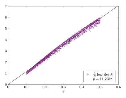
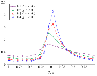
Figure 1: (Left) The quantity $\frac{2}{N}\log|\det J(z(x,\tau))|$ obtained for each configuration is plotted against $\tau$ for $N=9$. The solid line represents a fit to a linear function $c\,\tau$, where $c=11.795$. (Right) The phase distribution of the reweighting factor in (4.2) is plotted for configurations with the value of $\tau$ in various regions for $N=9$.

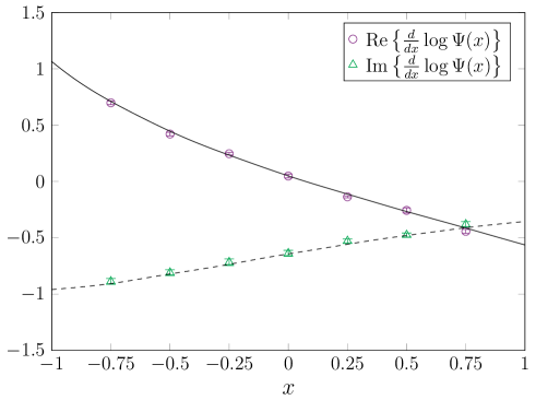
Figure 2: The real and imaginary parts of the log derivative of the wave function after time evolution with $t_{\rm f}=2$ is plotted for $N=9$. The solid line (real part) and the dashed line (imaginary part) represent the results obtained by diagonalizing the Hamiltonian, which corresponds to $N=\infty$.

We consider the time evolution for $t_{\rm f}=2$, which is discretized by $N=9$. The flow equation is discretized with $N_{\tau}=10$ steps. In the HMC algorithm, we use $N_{s}=15$ steps with the total fictitious time $s_{\rm f}=0.25$. We have confirmed that the computational cost for making one step in the HMC algorithm scales linearly with $N$.

In Fig. 1 (Left), we plot $\frac{2}{N}\log|\det J(z(x,\tau))|$ obtained for each configuration against $\tau$. We can fit the data points to a linear function $c\,\tau$ with $c=11.795$, which is consistent with the fact that the typical scale factor between the original and deformed contours grows exponentially with the flow time $\tau$. According to our discussion in Section 6.1, we therefore use $m(\tau)=e^{c\,\tau}$ in the Hamiltonian (6.2). In reweighting (4.2), we choose $\widetilde{W}(\tau)=\frac{1}{2}\,N\,c\,\tau$ in order to cancel the reweighting factor $|\det J(x,\tau)|\sim m(\tau)^{N/2}$. In Fig. 1 (Right), we plot the phase distribution of the reweighting factor (4.2) for configurations obtained within various regions of $\tau$. We find that the peak of the distribution becomes sharper as one goes to larger $\tau$, which confirms that the sign problem becomes weaker as $\tau$ increases.

Instead of calculating the time-evolved wave function (6.17) directly, we calculate its log derivative by

$$\frac{\partial}{\partial x_{\rm f}}\log\Psi(x_{\rm f},t_{\rm f}) =-\left\langle\frac{\partial}{\partial x_{\rm f}}f(x_{N},x_{\rm f})\right\rangle_{x_{\rm f}}\ ,$$ (6.23)

where the expectation value is taken with respect to the partition function (6.20). The results for $N=9$ are shown in Fig. 2, which is in good agreement with the results obtained by diagonalizing the Hamiltonian that corresponds to a continuous time evolution ($N=\infty$).

7 Summary and discussions

In this paper, we have proposed a new HMC algorithm for fast Lefschetz thimble calculations. Unlike the existing HMC algorithms, which solve the Hamilton dynamics on the deformed contour, we solve the Hamilton dynamics on the original contour using the action evaluated at the point obtained by solving the holomorphic gradient flow equation. The crucial point of our proposal is to calculate the force in the Hamilton dynamics by backpropagating the force on the deformed contour to that on the original contour, analogously to the well-known idea that plays a central role in machine learning. The computational cost in the present calculation is reduced by a factor of the system size.

The possible ergodicity problem can be avoided by integrating over the flow time [30], which can be naturally implemented in our algorithm. We discussed, in particular, that the flow equation can be discretized even in this case without causing systematic errors unlike the existing HMC algorithms. We have also discussed the relationship to the existing HMC algorithms from the viewpoint of the Hamilton dynamics, which revealed the existence of a nontrivial kernel in the kinetic term. This kernel actually reproduces the volume element of the deformed manifold upon integrating the auxiliary momentum variables. Inspired by this observation, we introduced a flow-time dependent mass parameter in the Hamilton dynamics, which turns out to be important in practical applications.

Our algorithm is particularly useful in identifying the saddle points and the associated thimbles that contribute to the integral in question. This may shed light, for instance, on quantum tunneling phenomena from the viewpoint of the real-time path integral [40, 41, 42, 43, 44]. On the other hand, when one calculates the expectation values, one needs to calculate the Jacobian that appears in the reweighting factor. This is time-consuming, but it can be done off-line only when one measures the observables. If one uses a crude estimator of the Jacobian whose cost is only proportional to the system size [33], the computational cost becomes comparable to ordinary Monte Carlo simulation for positive semi-definite weights. We hope to apply our algorithm to a large system in that way, although it would be certainly nice if there is a better way to treat the Jacobian.

Last but not the least, the “original contour” in our algorithm does not have to be the real axis but can be deformed in the complex plane as far as one does not pass through singularities. This points to the possibility of combining the GTM with various proposals for path optimization [45, 46, 47, 48, 49, 50, 51, 52], which may be useful in reducing the flow time required to solve the sign problem, and hence in reducing the effects of the Jacobian in reweighting.

Acknowledgements

We would like to thank Yuhma Asano, Masafumi Fukuma, Yuta Ito, Akira Matsumoto, Nobuyuki Matsumoto and Neill C. Warrington for valuable discussions. The computations were carried out on the PC clusters in KEK Computing Research Center and KEK Theory Center. K. S. is supported by the Grant-in-Aid for JSPS Research Fellow, No. 20J00079.

Appendix A Comments on the reduction of computational cost

In this appendix, we provide a simple understanding for the reduction of computational cost by backpropagation.

Let us first rewrite the differential equation (2.7) as

$$\frac{\partial}{\partial\sigma}\begin{pmatrix}J(x,\sigma)\\ \bar{J}(x,\sigma)\end{pmatrix} ={\cal H}(\sigma)\begin{pmatrix}J(x,\sigma)\\ \bar{J}(x,\sigma)\end{pmatrix}\ ,$$ (A.1)

where we have defined the $2N\times 2N$ matrix ${\cal H}(\sigma)$ as

$${\cal H}(\sigma) =\begin{pmatrix}&\overline{H(z(x,\sigma))}\\ H(z(x,\sigma))&\end{pmatrix}\ .$$ (A.2)

The solution to the differential equation (A.1) can be written down formally as

$$\begin{pmatrix}J(x,\tau)\\ \bar{J}(x,\tau)\end{pmatrix} ={\cal P}\exp\left(\int_{0}^{\tau}d\sigma\,{\cal H}(\sigma)\right)\begin{pmatrix}{\bf 1}_{N}\\ {\bf 1}_{N}\end{pmatrix}\ ,$$ (A.3)

where ${\bf 1}_{N}$ is the $N\times N$ unit matrix, and ${\cal P}\exp$ represents the path-ordered exponential, which ensures that ${\cal H}(\sigma)$ with smaller $\sigma$ comes on the right after Taylor expansion. On the other hand, $F_{j}$ defined by (3.9) can be written as

$$F^{\top} =\begin{pmatrix}f^{\top}&\bar{f}\,{}^{\top}\end{pmatrix}\begin{pmatrix}J(x,\tau)\\ \bar{J}(x,\tau)\end{pmatrix}\ .$$ (A.4)

Plugging (A.3) in (A.4), we obtain

$$F^{\top} =\begin{pmatrix}f^{\top}&\bar{f}\,{}^{\top}\end{pmatrix}{\cal P}\exp\left(\int_{0}^{\tau}d\sigma\,{\cal H}(\sigma)\right)\begin{pmatrix}{\bf 1}_{N}\\ {\bf 1}_{N}\end{pmatrix}\ .$$ (A.5)

A naive method would be to obtain the Jacobian by (A.3) and to obtain $F_{j}$ by (A.4), which corresponds to taking the products in (A.5) from the right.

Let us consider how the backpropagation calculates the same quantity (A.5). First, the “force” $f_{i}(\sigma)$ at flow time $\sigma$ defined by (3.12) can be written as

$$\begin{pmatrix}f^{\top}(\sigma)&\bar{f}{}^{\,\top}(\sigma)\end{pmatrix} =\begin{pmatrix}f^{\top}&\bar{f}{}^{\,\top}\end{pmatrix}{\cal P}\exp\left(\int_{\sigma}^{\tau}d\tilde{\sigma}\,{\cal H}(\tilde{\sigma})\right)\ .$$ (A.6)

This quantity satisfies the differential equation

$$\frac{d}{d\sigma}\begin{pmatrix}f^{\top}(\sigma)&\bar{f}{}^{\,\top}(\sigma)\end{pmatrix} =-\begin{pmatrix}f^{\top}(\sigma)&\bar{f}{}^{\,\top}(\sigma)\end{pmatrix}{\cal H}(\sigma)\ ,$$ (A.7)

which is equivalent to (3.15). By solving this backwards in $\sigma$ from $\sigma=\tau$ to $\sigma=0$ with the initial condition $f_{j}(\tau)=f_{j}$, we obtain

$$\begin{pmatrix}f^{\top}(0)&\bar{f}{}^{\,\top}(0)\end{pmatrix} =\begin{pmatrix}f^{\top}&\bar{f}{}^{\,\top}\end{pmatrix}{\cal P}\exp\left(\int_{0}^{\tau}d\tilde{\sigma}\,{\cal H}(\tilde{\sigma})\right)\ .$$ (A.8)

Using this in (A.5), we obtain

$$F^{\top} =\begin{pmatrix}f^{\top}(0)&\bar{f}{}^{\,\top}(0)\end{pmatrix}\begin{pmatrix}{\bf 1}_{N}\\ {\bf 1}_{N}\end{pmatrix}=f^{\top}(0)+\bar{f}{}^{\,\top}(0)\ .$$ (A.9)

Thus, the backpropagation amounts to reversing the order of multiplications in (A.5), which replaces the matrix-matrix products by the matrix-vector products, thereby reducing the computational cost by a factor of O($N$).

The point just mentioned becomes clearer in the case of discretized flow time discussed in Section 3.3. Corresponding to (A.1), we can rewrite (3.19) in the form

$$\begin{pmatrix}J(x,\sigma_{n+1})\\ \bar{J}(x,\sigma_{n+1})\end{pmatrix} =\Big{\{}1+\varepsilon\,{\cal H}(\sigma_{n})\Big{\}}\begin{pmatrix}J(x,\sigma_{n})\\ \bar{J}(x,\sigma_{n})\end{pmatrix}\ ,$$ (A.10)

where the $2N\times 2N$ matrix ${\cal H}(\sigma)$ is defined by (A.2) as before. The formal solution corresponding to (A.3) can be written as

$$\begin{pmatrix}J(x,\tau)\\ \bar{J}(x,\tau)\end{pmatrix} =\prod_{k=1}^{N_{\tau}}\Big{\{}1+\varepsilon\,{\cal H}(\sigma_{k-1})\Big{\}}\begin{pmatrix}{\bf 1}_{N}\\ {\bf 1}_{N}\end{pmatrix}\ ,$$ (A.11)

where the product is taken in such a way that a factor with smaller $k$ comes on the right. Plugging (A.11) in (A.4), we obtain

$$F^{\top} =\begin{pmatrix}f^{\top}&\bar{f}\,{}^{\top}\end{pmatrix}\prod_{k=1}^{N_{\tau}}\Big{\{}1+\varepsilon\,{\cal H}(\sigma_{k-1})\Big{\}}\begin{pmatrix}{\bf 1}_{N}\\ {\bf 1}_{N}\end{pmatrix}\ .$$ (A.12)

Corresponding to (A.6), let us define

$$\begin{pmatrix}f^{\top}(\sigma_{n})&\bar{f}{}^{\,\top}(\sigma_{n})\end{pmatrix} =\begin{pmatrix}f^{\top}&\bar{f}^{\,\top}\end{pmatrix}\prod_{k=n+1}^{N_{\tau}}\Big{\{}1+\varepsilon\,{\cal H}(\sigma_{k-1})\Big{\}}\ ,$$ (A.13)

which represents the force propagated backwards in $\sigma$. Note that this quantity satisfies the difference equation

$$\begin{pmatrix}f^{\top}(\sigma_{n-1})&\bar{f}{}^{\,\top}(\sigma_{n-1})\end{pmatrix}=\begin{pmatrix}f^{\top}(\sigma_{n})&\bar{f}{}^{\,\top}(\sigma_{n})\end{pmatrix}\Big{\{}1+\varepsilon\,{\cal H}(\sigma_{n-1})\Big{\}}\ ,$$ (A.14)

which is equivalent to (3.22). By solving this difference equation with the initial condition $f_{j}(\tau)=f_{j}$, we obtain the desired force as (3.17). Thus, in the discretized version, the backpropagation simply amounts to taking the products in (A.12) from the left, which reduces the cost by a factor of O($N$) compared with taking the products from the right.

Appendix B Some basic properties of the deformed manifold

In this appendix, we briefly review some basic properties of the deformed manifold [30], which is necessary in understanding Section 5. We also provide a proof for the statement (5.17).

The deformed manifold consists of points $z_{i}(x)$, which can be obtained by solving either the continuous or discretized version of the holomorphic gradient flow equation for the flow time $\tau=x_{0}$ with the initial point given by $x_{i}$. Therefore, the deformed manifold is parametrized by $x_{\mu}$ ($\mu=0,1,\cdots,N$), and it is embedded in ${\mathbb{C}}^{N}$. As we mentioned in Section 5, our discussion applies to the case of fixed $\tau$ as well by replacing the index $\mu=0,1,\cdots,N$ with $i=1,\cdots,N$.

The tangent space at each point on the deformed manifold is a real linear space spanned by the basis vectors

$$E_{\mu}^{\,i} =\frac{\partial z_{i}}{\partial x_{\mu}}\ ,$$ (B.1)

and any element of it can be represented as

$$v_{i} =c_{\mu}E_{\mu}^{\,i}\ ,\quad\quad\mbox{where $c_{\mu}\in{\mathbb{R}}$}\ .$$ (B.2)

Since the deformed manifold is embedded in ${\mathbb{C}}^{N}$, one can define the inner product of two tangent vectors $u_{i}$ and $v_{i}$ as

$$\langle u,v\rangle ={\rm Re}\left(\bar{u}_{i}v_{i}\right)\ .$$ (B.3)

Expanding the tangent vector $v_{i}$ as (B.2) and similarly for $u_{i}$ as

$$u_{i} =b_{\mu}E_{\mu}^{\,i}\ ,$$ (B.4)

we can rewrite the inner product $\langle u,v\rangle$ in terms of the coefficients $b_{\mu}$ and $c_{\mu}$ as

$$\langle u,v\rangle =g_{\mu\nu}b_{\mu}c_{\nu}\ ,$$ (B.5)

where $g_{\mu\nu}$ is defined by

$$g_{\mu\nu} ={\rm Re}\left(\overline{E_{\mu}^{\,i}}\,E_{\nu}^{\,i}\right)\ ,$$ (B.6)

which gives the induced metric (5.10) on the deformed manifold.

Let us consider a vector $w\in{\mathbb{C}}^{N}$ and project it onto the tangent space. For that, let us we decompose $w$ as

$$w_{i} =a_{\mu}E_{\mu}^{\,i}+y_{i}\ ,$$ (B.7)

where $a_{\mu}\in{\mathbb{R}}$ is specified later, and $y_{i}$ is a vector orthogonal to the tangent space; i.e.,

$${\rm Re}\left(\overline{E_{\mu}^{\,i}}\,y_{i}\right) =0\quad\quad\mbox{for all $\mu$}\ .$$ (B.8)

From (B.7), we obtain

$${\rm Re}\left(\overline{E_{\mu}^{\,i}}\,w_{i}\right) =a_{\nu}{\rm Re}\left(\overline{E_{\mu}^{\,i}}\,E_{\nu}^{\,i}\right)$$ (B.9)

$$=g_{\mu\nu}a_{\nu}\ .$$ (B.10)

Thus one obtains

$$a_{\mu} =(g^{-1})_{\mu\nu}{\rm Re}\left(\overline{E_{\nu}^{\,i}}\,w_{i}\right)\ .$$ (B.11)

Plugging this in (B.7), the projection of $w$ onto the tangent space is given by

$$w_{i}\mapsto w_{i}^{\prime} =E_{\mu}^{\,i}(g^{-1})_{\mu\nu}{\rm Re}\left(\overline{E_{\nu}^{\,j}}\,w_{j}\right)\ .$$ (B.12)

This confirms that (5.16) is indeed the projection of the gradient force $-\frac{\partial V(z,\bar{z})}{\partial\bar{z}_{i}}$ onto the tangent space.

Let us next prove (5.17). The left-hand side can be written as

$${\rm Re}\left(\overline{\frac{\partial z_{i}}{\partial x_{\alpha}}}\,{\cal N}_{i}^{\prime}\right) =p_{\lambda}{\cal M}_{\lambda\rho,\alpha}p_{\rho}\ ,$$ (B.13)

where ${\cal M}_{\lambda\rho,\alpha}$ is defined by

$${\cal M}_{\lambda\rho,\alpha}= -\frac{1}{2}g_{\alpha\mu}K_{\mu\nu}\frac{\partial K_{\lambda\rho}}{\partial x_{\nu}}+\frac{1}{2}K_{\nu\rho}g_{\alpha\mu}\frac{\partial K_{\mu\lambda}}{\partial x_{\nu}}+\frac{1}{2}K_{\nu\lambda}g_{\alpha\mu}\frac{\partial K_{\mu\rho}}{\partial x_{\nu}}$$

$$+{\rm Re}\left(\overline{\frac{\partial z_{i}}{\partial x_{\alpha}}}\frac{\partial^{2}z_{i}}{\partial x_{\mu}\partial x_{\nu}}\right)K_{\nu\lambda}K_{\mu\rho}\ .$$ (B.14)

Let us recall here that $K=\frac{1}{2}\,g^{-1}$, which implies that

$$g_{\alpha\mu}K_{\mu\nu}\frac{\partial K_{\lambda\rho}}{\partial x_{\nu}} =\frac{1}{2}\frac{\partial K_{\lambda\rho}}{\partial x_{\alpha}}=-K_{\lambda\nu}\frac{\partial g_{\mu\nu}}{\partial x_{\alpha}}K_{\mu\rho}\ ,$$ (B.15)

$$g_{\alpha\mu}\frac{\partial K_{\mu\lambda}}{\partial x_{\nu}} =-\frac{\partial g_{\alpha\mu}}{\partial x_{\nu}}K_{\mu\lambda}\ .$$ (B.16)

Using the definition (5.10) of the induced metric, we obtain

$$\frac{\partial g_{\alpha\mu}}{\partial x_{\nu}} ={\rm Re}\left(\frac{\partial^{2}z_{i}}{\partial x_{\nu}\partial x_{\alpha}}\overline{\frac{\partial z_{i}}{\partial x_{\mu}}}+\frac{\partial^{2}z_{i}}{\partial x_{\mu}\partial x_{\nu}}\overline{\frac{\partial z_{i}}{\partial x_{\alpha}}}\right)\ .$$ (B.17)

Thus (B.14) becomes

$${\cal M}_{\lambda\rho,\alpha}= K_{\nu\lambda}K_{\mu\rho}\!\left\{\frac{1}{2}{\rm Re}\!\left(\frac{\partial^{2}z_{i}}{\partial x_{\mu}\partial x_{\alpha}}\overline{\frac{\partial z_{i}}{\partial x_{\nu}}}+\frac{\partial^{2}z_{i}}{\partial x_{\nu}\partial x_{\alpha}}\overline{\frac{\partial z_{i}}{\partial x_{\mu}}}\right)\!-\!\frac{1}{2}{\rm Re}\!\left(\frac{\partial^{2}z_{i}}{\partial x_{\mu}\partial x_{\alpha}}\overline{\frac{\partial z_{i}}{\partial x_{\nu}}}+\frac{\partial^{2}z_{i}}{\partial x_{\mu}\partial x_{\nu}}\overline{\frac{\partial z_{i}}{\partial x_{\alpha}}}\right)\right.$$

$$\quad\quad\quad\quad\left.-\frac{1}{2}{\rm Re}\left(\frac{\partial^{2}z_{i}}{\partial x_{\nu}\partial x_{\alpha}}\overline{\frac{\partial z_{i}}{\partial x_{\mu}}}+\frac{\partial^{2}z_{i}}{\partial x_{\mu}\partial x_{\nu}}\overline{\frac{\partial z_{i}}{\partial x_{\alpha}}}\right)+{\rm Re}\left(\frac{\partial^{2}z_{i}}{\partial x_{\mu}\partial x_{\nu}}\overline{\frac{\partial z_{i}}{\partial x_{\alpha}}}\right)\right\}=0\ ,$$ (B.18)

which completes the proof.

Appendix C Violation of ${\rm Im}(J^{\dagger}J)=0$ for the discretized flow

In this section, we point out that ${\rm Im}(J^{\dagger}J)=0$ holds only for the continuous flow but not for the discretized one. For the continuous flow equation, one obtains from (2.7),

$$\frac{\partial}{\partial\sigma}(J^{\dagger}J)_{ij}(x,\sigma) =\overline{J_{ki}(x,\sigma)}\,\overline{H_{kl}(z(x,\sigma))}\,\overline{J_{lj}(x,\sigma)}+J_{ki}(x,\sigma)\,H_{kl}(z(x,\sigma))\,J_{lj}(x,\sigma)$$

$$=2\,{\rm Re}\left\{J_{ki}(x,\sigma)\,H_{kl}(z(x,\sigma))\,J_{lj}(x,\sigma)\right\}\ ,$$ (C.1)

which implies that $(J^{\dagger}J)_{ij}(x,\sigma)\in{\mathbb{R}}$ due to the initial condition $(J^{\dagger}J)_{ij}(x,0)=\delta_{ij}$.

Note that in the first equality of (C.1), we need to use the Leibniz rule, which is violated upon discretization of the flow equation. Namely, we obtain

$$(J^{\dagger}J)_{ij}(x,\sigma_{n+1})$$

$$= \left\{\overline{J_{ki}(x,\sigma_{n})}+\varepsilon\,J_{mi}(x,\sigma_{n})\,H_{mk}(z(x,\sigma_{n}))\right\}\left\{J_{kj}(x,\sigma_{n_{n}})+\varepsilon\,\overline{H_{kl}(z(x,\sigma_{n}))}\,\overline{J_{lj}(x,\sigma_{n})}\right\}$$

$$= (J^{\dagger}J)_{ij}(x,\sigma_{n})+2\,\varepsilon\,{\rm Re}\left\{J_{mi}(x,\sigma_{n})\,H_{mk}(z(x,\sigma_{n}))\,J_{kj}(x,\sigma_{n_{n}})\right\}$$

$$+\varepsilon^{2}\,J_{mi}(x,\sigma_{n})\,H_{mk}(z(x,\sigma_{n}))\,\overline{H_{kl}(z(x,\sigma_{n}))}\,\overline{J_{lj}(x,\sigma_{n})}\ ,$$ (C.2)

where the last term on the right-hand side is not necessarily real. Therefore, $(J^{\dagger}J)_{ij}(x,\sigma_{n})$ is not real at the discretized level.

References

- [1] M. Levin and C. P. Nave, Tensor renormalization group approach to 2d classical lattice models, Phys.Rev.Lett. 99 (2007), no. 12 120601, [cond-mat/0611687].
- [2] Z. Y. Xie, J. Chen, M. P. Qin, J. W. Zhu, L. P. Yang, and T. Xiang, Coarse-graining renormalization by higher-order singular value decomposition, Phys. Rev. B 86 (Jul, 2012) 045139.
- [3] G. Evenbly and G. Vidal, Tensor network renormalization, Phys. Rev. Lett. 115 (Oct, 2015) 180405.
- [4] D. Adachi, T. Okubo, and S. Todo, Anisotropic Tensor Renormalization Group, Phys. Rev. B 102 (2020), no. 5 054432, [arXiv:1906.02007].
- [5] D. Kadoh and K. Nakayama, Renormalization group on a triad network, arXiv:1912.02414.
- [6] J. R. Klauder, Coherent state Langevin equations for canonical quantum systems with applications to the quantized Hall effect, Phys. Rev. A29 (1984) 2036–2047.
- [7] G. Parisi, On complex probabilities, Phys. Lett. 131B (1983) 393–395.
- [8] G. Aarts, E. Seiler, and I.-O. Stamatescu, The Complex Langevin method: When can it be trusted?, Phys. Rev. D81 (2010) 054508, [arXiv:0912.3360].
- [9] G. Aarts, F. A. James, E. Seiler, and I.-O. Stamatescu, Complex langevin: Etiology and diagnostics of its main problem, Eur.Phys.J.C 71 (2011) 1756, [arXiv:1101.3270].
- [10] K. Nagata, J. Nishimura, and S. Shimasaki, Justification of the complex Langevin method with the gauge cooling procedure, PTEP 2016 (2016), no. 1 013B01, [arXiv:1508.02377].
- [11] K. Nagata, J. Nishimura, and S. Shimasaki, Argument for justification of the complex Langevin method and the condition for correct convergence, Phys. Rev. D94 (2016), no. 11 114515, [arXiv:1606.07627].
- [12] D. Sexty, Calculating the equation of state of dense quark-gluon plasma using the complex Langevin equation, Phys. Rev. D 100 (2019), no. 7 074503, [arXiv:1907.08712].
- [13] C. E. Berger, L. Rammelmüller, A. C. Loheac, F. Ehmann, J. Braun, and J. E. Drut, Complex Langevin and other approaches to the sign problem in quantum many-body physics, Phys. Rept. 892 (2021) 1–54, [arXiv:1907.10183].
- [14] K. N. Anagnostopoulos, T. Azuma, Y. Ito, J. Nishimura, T. Okubo, and S. Kovalkov Papadoudis, Complex Langevin analysis of the spontaneous breaking of 10D rotational symmetry in the Euclidean IKKT matrix model, JHEP 06 (2020) 069, [arXiv:2002.07410].
- [15] M. Scherzer, D. Sexty, and I. O. Stamatescu, Deconfinement transition line with the complex Langevin equation up to , Phys. Rev. D 102 (2020), no. 1 014515, [arXiv:2004.05372].
- [16] F. Attanasio, B. Jäger, and F. P. G. Ziegler, Complex Langevin simulations and the QCD phase diagram: Recent developments, Eur. Phys. J. A 56 (2020), no. 10 251, [arXiv:2006.00476].
- [17] Y. Ito, H. Matsufuru, Y. Namekawa, J. Nishimura, S. Shimasaki, A. Tsuchiya, and S. Tsutsui, Complex Langevin calculations in QCD at finite density, JHEP 10 (2020) 144, [arXiv:2007.08778].
- [18] I. Aniceto, G. Basar, and R. Schiappa, A Primer on Resurgent Transseries and Their Asymptotics, Phys. Rept. 809 (2019) 1–135, [arXiv:1802.10441].
- [19] J. Feldbrugge, J.-L. Lehners, and N. Turok, Lorentzian Quantum Cosmology, Phys. Rev. D 95 (2017), no. 10 103508, [arXiv:1703.02076].
- [20] D. Jia, Complex, Lorentzian, and Euclidean simplicial quantum gravity: numerical methods and physical prospects, arXiv:2110.05953.
- [21] E. Witten, Analytic continuation of Chern-Simons theory, AMS/IP Stud. Adv. Math. 50 (2011) 347–446, [arXiv:1001.2933].
- [22] AuroraScience Collaboration, M. Cristoforetti, F. Di Renzo, and L. Scorzato, New approach to the sign problem in quantum field theories: High density qcd on a lefschetz thimble, Phys.Rev.D 86 (2012) 074506, [arXiv:1205.3996].
- [23] M. Cristoforetti, F. Di Renzo, A. Mukherjee, and L. Scorzato, Monte Carlo simulations on the Lefschetz thimble: Taming the sign problem, Phys. Rev. D 88 (2013), no. 5 051501, [arXiv:1303.7204].
- [24] H. Fujii, D. Honda, M. Kato, Y. Kikukawa, S. Komatsu, and T. Sano, Hybrid monte carlo on lefschetz thimbles - a study of the residual sign problem, JHEP 10 (2013) 147, [arXiv:1309.4371].
- [25] A. Alexandru, G. Basar, P. F. Bedaque, G. W. Ridgway, and N. C. Warrington, Sign problem and monte carlo calculations beyond lefschetz thimbles, JHEP 05 (2016) 053, [arXiv:1512.08764].
- [26] A. Alexandru, G. Basar, P. F. Bedaque, G. W. Ridgway, and N. C. Warrington, Monte Carlo calculations of the finite density Thirring model, Phys. Rev. D 95 (2017), no. 1 014502, [arXiv:1609.01730].
- [27] M. Fukuma and N. Umeda, Parallel tempering algorithm for integration over lefschetz thimbles, PTEP 2017 (2017), no. 7 073B01, [arXiv:1703.00861].
- [28] A. Alexandru, G. Basar, P. F. Bedaque, and N. C. Warrington, Tempered transitions between thimbles, Phys. Rev. D 96 (2017), no. 3 034513, [arXiv:1703.02414].
- [29] M. Fukuma, N. Matsumoto, and N. Umeda, Implementation of the HMC algorithm on the tempered Lefschetz thimble method, arXiv:1912.13303.
- [30] M. Fukuma and N. Matsumoto, Worldvolume approach to the tempered Lefschetz thimble method, PTEP 2021 (2021), no. 2 023B08, [arXiv:2012.08468].
- [31] A. Alexandru, G. Basar, P. F. Bedaque, and N. C. Warrington, Complex Paths Around The Sign Problem, arXiv:2007.05436.
- [32] M. Ulybyshev, C. Winterowd, and S. Zafeiropoulos, Lefschetz thimbles decomposition for the Hubbard model on the hexagonal lattice, Phys. Rev. D 101 (2020), no. 1 014508, [arXiv:1906.07678].
- [33] A. Alexandru, G. Basar, P. F. Bedaque, G. W. Ridgway, and N. C. Warrington, Fast estimator of Jacobians in the Monte Carlo integration on Lefschetz thimbles, Phys. Rev. D 93 (2016), no. 9 094514, [arXiv:1604.00956].
- [34] S. Duane, A. D. Kennedy, B. J. Pendleton, and D. Roweth, Hybrid Monte Carlo, Phys. Lett. B 195 (1987) 216–222.
- [35] A. Tomiya and Y. Nagai, Gauge covariant neural network for 4 dimensional non-abelian gauge theory, arXiv:2103.11965.
- [36] M. Fukuma, N. Matsumoto, and Y. Namekawa, Statistical analysis method for the worldvolume hybrid Monte Carlo algorithm, PTEP 2021 (2021), no. 12 123B02, [arXiv:2107.06858].
- [37] A. Alexandru, G. Basar, P. F. Bedaque, S. Vartak, and N. C. Warrington, Monte Carlo Study of Real Time Dynamics on the Lattice, Phys. Rev. Lett. 117 (2016), no. 8 081602, [arXiv:1605.08040].
- [38] A. Alexandru, G. Basar, P. F. Bedaque, and G. W. Ridgway, Schwinger-Keldysh formalism on the lattice: A faster algorithm and its application to field theory, Phys. Rev. D 95 (2017), no. 11 114501, [arXiv:1704.06404].
- [39] Z.-G. Mou, P. M. Saffin, A. Tranberg, and S. Woodward, Real-time quantum dynamics, path integrals and the method of thimbles, JHEP 06 (2019) 094, [arXiv:1902.09147].
- [40] N. Turok, On Quantum Tunneling in Real Time, New J. Phys. 16 (2014) 063006, [arXiv:1312.1772].
- [41] Y. Tanizaki and T. Koike, Real-time Feynman path integral with Picard–Lefschetz theory and its applications to quantum tunneling, Annals Phys. 351 (2014) 250–274, [arXiv:1406.2386].
- [42] A. Cherman and M. Unsal, Real-Time Feynman Path Integral Realization of Instantons, arXiv:1408.0012.
- [43] S. F. Bramberger, G. Lavrelashvili, and J.-L. Lehners, Quantum tunneling from paths in complex time, Phys. Rev. D 94 (2016), no. 6 064032, [arXiv:1605.02751].
- [44] Z.-G. Mou, P. M. Saffin, and A. Tranberg, Quantum tunnelling, real-time dynamics and Picard-Lefschetz thimbles, JHEP 11 (2019) 135, [arXiv:1909.02488].
- [45] Y. Mori, K. Kashiwa, and A. Ohnishi, Toward solving the sign problem with path optimization method, Phys. Rev. D 96 (2017), no. 11 111501, [arXiv:1705.05605].
- [46] Y. Mori, K. Kashiwa, and A. Ohnishi, Application of a neural network to the sign problem via the path optimization method, PTEP 2018 (2018), no. 2 023B04, [arXiv:1709.03208].
- [47] A. Alexandru, P. F. Bedaque, H. Lamm, and S. Lawrence, Finite-Density Monte Carlo Calculations on Sign-Optimized Manifolds, Phys. Rev. D 97 (2018), no. 9 094510, [arXiv:1804.00697].
- [48] F. Bursa and M. Kroyter, A simple approach towards the sign problem using path optimisation, JHEP 12 (2018) 054, [arXiv:1805.04941].
- [49] K. Kashiwa, Y. Mori, and A. Ohnishi, Controlling the model sign problem via the path optimization method: Monte Carlo approach to a QCD effective model with Polyakov loop, Phys. Rev. D 99 (2019), no. 1 014033, [arXiv:1805.08940].
- [50] A. Alexandru, P. F. Bedaque, H. Lamm, S. Lawrence, and N. C. Warrington, Fermions at Finite Density in 2+1 Dimensions with Sign-Optimized Manifolds, Phys. Rev. Lett. 121 (2018), no. 19 191602, [arXiv:1808.09799].
- [51] W. Detmold, G. Kanwar, M. L. Wagman, and N. C. Warrington, Path integral contour deformations for noisy observables, Phys. Rev. D 102 (2020), no. 1 014514, [arXiv:2003.05914].
- [52] W. Detmold, G. Kanwar, H. Lamm, M. L. Wagman, and N. C. Warrington, Path integral contour deformations for observables in gauge theory, Phys. Rev. D 103 (2021), no. 9 094517, [arXiv:2101.12668].