Primordial black holes and scalar induced gravitational waves from the $E$ model with a Gauss-Bonnet term

Abstract

We study an inflationary $E$ model with the Gauss-Bonnet coupling, which can enhance the curvature perturbation at small scales and thus produce a significant abundance of primordial black holes (PBHs) and detectable scalar induced gravitational waves (SIGWs). PBHs from the $E$ model with mass $30M_{\odot}$, $10^{-5}M_{\odot}$, and $10^{-12}M_{\odot}$ can explain the LIGO-Virgo events, the ultrashort-timescale microlensing events in the OGLE data, and all dark matter, respectively. SIGWs produced by the $E$ model can account for the recent NANOGrav signal. We also compute the primordial non-Gaussianity and discuss its impact on PBHs and SIGWs. The probability distribution of density contrast is modified to be right-tailed, which we find prompts the formation of PBHs, so that the abundance of PBHs is underestimated with Gaussian approximation. On the contrary, the fractional energy density of SIGWs is hardly affected.

I Introduction

The primordial black hole (PBH) Carr and Hawking (1974); Hawking (1971) dark matter (DM) has revived the research interests of the community since the detection of gravitational waves (GWs) by the Laser Interferometer Gravitational-Wave Observatory (LIGO) scientific collaboration and Virgo collaboration Abbott et al. (2016a, b, 2017a, 2017b, 2017c, 2017d, 2019, 2020a, 2020b, 2020c), as the GW events may originate from PBHs Bird et al. (2016); Sasaki et al. (2016); Takhistov et al. (2021); De Luca et al. (2021a); Abbott et al. (2021).

The gravitational collapse of the overdense region in the early Universe, especially in the radiation-dominated era, is one of the most accepted mechanisms to produce PBHs. The large density perturbations generated during inflationary era induce the gravitational collapse after horizon reentry. In addition to PBHs, these perturbations also induce the generation of scalar induced gravitational waves (SIGWs) that contribute to the stochastic gravitational wave background (SGWB) Saito and Yokoyama (2009); Orlofsky et al. (2017); Nakama et al. (2017); Wang et al. (2018); Cai et al. (2019); Kohri and Terada (2018); Espinosa et al. (2018); Kuroyanagi et al. (2018); Domènech (2020); Fumagalli et al. (2021); Domènech et al. (2020); Domènech (2021); Wang and Kohri (2021); Adshead et al. (2021); Ahmed et al. (2021). In order to produce PBHs occupying a significant portion of dark matter, the power spectrum of curvature perturbations should be enhanced to $\mathcal{P}_{\mathcal{R}}\sim\mathcal{O}(10^{-2})$ on small scales Motohashi and Hu (2017); Sato-Polito et al. (2019); Lu et al. (2019); Khlopov (2010), seven-order larger than the cosmic microwave background (CMB) constraint, that is, $\mathcal{P}_{\mathcal{R}}\sim\mathcal{O}(10^{-9})$ on large scales Akrami et al. (2020).

Some inflationary models, such as the canonical single-field inflation with an inflection point Germani and Prokopec (2017); Di and Gong (2018); Garcia-Bellido and Ruiz Morales (2017); Xu et al. (2020), or a steplike feature Inomata et al. (2021) in potential can realize the enhancement of power spectrum. Besides, a single-field inflaton with a noncanonical kinetic term that contains a peaked coupling function is also an efficient way to amplify the power spectrum Lin et al. (2020); Yi et al. (2021a, b); Gao et al. (2021); Lin et al. (2021); Zhang et al. (2021a, b). Recently, the two-field inflation models that predict PBH dark matter and observable SIGWs also attract much attention Pi et al. (2018); Braglia et al. (2020); Cheong et al. (2021); Gundhi et al. (2021); Palma et al. (2020); Spanos and Stamou (2021); Cai et al. (2021).

Usually, the perturbation is assumed to be Gaussian in computing the abundance of PBHs. However, if non-Gaussianity parameter satisfies $f_{\mathrm{NL}}\gtrsim\mathcal{O}(0.01)$, then even an unobservable non-Gaussianity could result in a large correction to the Gaussian-predicted PBH abundance Zhang et al. (2021b). Several canonical single-field inflation models with an inflection point in the inflaton potential that serves the formation of PBHs have been reanalyzed Atal and Germani (2019). It was found that the effect of non-Gaussianity of primordial curvature perturbations on PBH abundance is non-negligible in these models. Some noncanonical inflationary models with minimal or nonminimal coupling between gravity and inflaton also produce non-Gaussianity that has a significant effect on PBH abundance Zhang et al. (2021b); Lin et al. (2021). In fact, these noncanonical inflation models are equivalent to canonical inflation models with an inflection point in potential by a conformal transformation and field redefinition Zhang et al. (2021b). Pedagogically, it is worth studying the inflationary models whose enhancement mechanism is different from that of the inflection-point inflations, and further discussing the effect of non-Gaussianity.

It is expected that the higher-order curvature correction of gravity plays an important role in the early Universe, for example, in the inflationary era. So, it is necessary to conceive an inflation model with higher-order curvature terms that give PBH dark matter and SIGWs. Based on this motivation, we consider an inflationary $E$ model with the Gauss-Bonnet term. The enhancement mechanism in this model is quite different from the inflection-point mechanism. Inflation with the Gauss-Bonnet term was widely studied Kawai and Soda (1999); Satoh and Soda (2008); Bamba et al. (2015, 2014); Nozari and Rashidi (2016, 2017); Yi et al. (2018); Kleidis and Oikonomou (2019); Pozdeeva (2020); Oikonomou and Fronimos (2021); Odintsov et al. (2020). It belongs to a subclass of the Horndeski theory, the most general scalar-tensor theory with the no-more-than-second-order equations of motion of both the metric and the scalar field Horndeski (1974); Kobayashi et al. (2011). It is interesting to see that if the Gauss-Bonnet term can lead to an amplification of the power spectrum of curvature perturbation. In Ref. Kawai and Kim (2021a), the authors use the natural potential to drive inflation with the Gauss-Bonnet term, and compute the PBH abundance with Gaussian approximation. As mentioned above, the PBH abundance is much sensitive to non-Gaussianity Zhang et al. (2021b), it is necessary to compute the non-Gaussianity and discuss its contribution to PBH abundance and corresponding SIGWs.

In this paper, we study the inflationary $E$ model with the Gauss-Bonnet coupling and compute the predicted PBH abundance and the fractional energy density of SIGWs. We also discuss the role that primordial non-Gaussianity plays in the generation of PBHs and SIGWs. This paper is organized as follows. In Sec. II, we compute the power spectrum from our model. In Sec. III, we compute the bispectrum and the corresponding non-Gaussianity parameter $f_{\mathrm{NL}}$. In Sec. IV, we compute the PBH abundance and the fractional energy density of SIGWs with consideration of non-Gaussianity of primordial curvature perturbations. Finally, we conclude this paper in Sec. V.

II The Gauss-Bonnet inflation

The action of the inflation model with the Gauss-Bonnet term is

$$S=\frac{1}{2}\int d^{4}x\sqrt{-g}\left[R-g^{\mu\nu}\partial_{\mu}\phi\partial_{\nu}\phi-2V(\phi)-\frac{1}{8}f(\phi)\mathcal{L}_{GB}\right],$$ (1)

where $\mathcal{L}_{GB}=R^{2}-4R_{\mu\nu}R^{\mu\nu}+R_{\mu\nu\rho\lambda}R^{\mu\nu\rho\lambda}$ is the Gauss-Bonnet term and $f(\phi)$ is a coupling function of inflaton $\phi$.

Working in the spatially flat Friedmann-Robertson-Walker metric and varying the action with respect to the metric $g_{\mu\nu}$ and the inflaton $\phi$, we get the following equations of motion

$$6H^{2}=\dot{\phi}^{2}+2V+3\dot{f}H^{3},$$ (2)

$$2\dot{H}=-\dot{\phi}^{2}+\frac{1}{2}\ddot{f}H^{2}+\frac{1}{2}\dot{f}H\left(2\dot{H}-H^{2}\right),$$ (3)

$$\ddot{\phi}+3H\dot{\phi}+V_{\phi}+\frac{3}{2}f_{\phi}H^{2}\left(\dot{H}+H^{2}\right)=0,$$ (4)

where the dot denotes the derivative with respect to $t$, and $f_{\phi}=df/d\phi$, $V_{\phi}=dV/d\phi$.

Impose the slow roll conditions, $\dot{\phi}^{2}\ll V(\phi)$, $H|\dot{f}|\ll 1$ and $|\ddot{f}|\ll H|\dot{f}|$, and the equation of motion for $\phi$ becomes

$$\ddot{\phi}+3H\dot{\phi}+V_{\phi}+\frac{1}{6}V^{2}f_{\phi}\simeq 0.$$ (5)

Conventionally, we assume that the acceleration of inflaton $\phi$ satisfies $-\ddot{\phi}/H\dot{\phi}\ll 1$ so that inflation lasts long enough. If the last two terms in Eq. (5) satisfy $V_{\phi}+V^{2}f_{\phi}/6\Big{|}_{\phi=\phi_{c}}\simeq 0$ at some energy scale $\phi_{c}$, then Eq. (5) becomes

$$\ddot{\phi}+3H\dot{\phi}\simeq 0,$$ (6)

which means the inflaton evolves into a transitory ultraslow-roll (USR) phase where the curvature perturbations is enhanced. This critical value $\phi_{c}$ is a nontrivial fixed point Kawai and Kim (2021b). So, this provides a way to adjust the parameters to realize an USR phase on different energy scales, which corresponds to an enhancement of power spectrum at different scales.

In this paper, we choose the coupling function to be Kawai and Kim (2021a)

$$f(\phi)=f_{0}\tanh[f_{1}(\phi-\phi_{c})],$$

and the $E$ model potential

$$V(\phi)=V_{0}\left[1-\mathrm{exp}{\left(-\sqrt{\frac{2}{3\alpha}}\phi\right)}\right]^{p},$$ (7)

where $\alpha$ and $p$ are two free parameters. For convenience, we define the Hubble flow parameters

$$\epsilon_{1}=-\frac{\dot{H}}{H^{2}},\ \ \epsilon_{2}=\frac{d\ln\epsilon_{1}}{Hdt},$$ (8)

similarly, for $f(\phi)$, we have

$$\xi_{1}=H\dot{f},\ \ \xi_{2}=\frac{d\ln\xi_{1}}{Hdt}.$$ (9)

The quadratic action that determines the evolution of comoving curvature perturbation is De Felice and Tsujikawa (2011a)

$$S_{2}=\int dtd^{3}xa^{3}Q\left(\dot{\mathcal{R}}^{2}-\frac{c^{2}_{s}}{a^{2}}(\partial\mathcal{R})^{2}\right),$$ (10)

where

$$Q=\frac{1}{2}\left(\frac{1-\xi_{1}/2}{1-3\xi_{1}/4}\right)^{2}\left(2\epsilon_{1}-\frac{1}{2}\xi_{1}+\frac{1}{2}\xi_{1}\xi_{2}-\frac{1}{2}\xi_{1}\epsilon_{1}+\frac{3}{4}\frac{\xi_{1}^{2}}{2-\xi_{1}}\right),$$ (11)

and

$$c^{2}_{s}=1-\frac{a^{2}}{z^{2}}\left(\frac{\xi_{1}}{2-3\xi_{1}/2}\right)^{2}\left(2\epsilon_{1}+\frac{1}{4}\xi_{1}-\frac{1}{4}\xi_{1}\xi_{2}-\frac{5}{4}\xi_{1}\epsilon_{1}\right),$$ (12)

with $z^{2}=2a^{2}Q$. The equation of motion for comoving curvature perturbation $\mathcal{R}$ reads

$$v^{{}^{\prime\prime}}_{k}+\left(c^{2}_{s}k^{2}-\frac{z^{{}^{\prime\prime}}}{z}\right)v_{k}=0,$$ (13)

where $v_{k}=z\mathcal{R}_{k}$ and $\mathcal{R}_{k}$ is the mode function. The prime denotes the derivative with respect to conformal time $\tau$.

The initial condition is given by Bunch-Davies vacuum. We numerically solve the equation (13) with the parameter sets in Table 1, and the results are shown in Tables 1, 2, and Fig. 1. From Table 1 and Fig. 1, the power spectra from the $E$ model satisfy the constraints on CMB Akrami et al. (2020); Ade et al. (2021) and the total $e$-folds $N_{*}\sim 60$. At small scales, the power spectra reach $\mathcal{O}(10^{-2})$ and satisfy the constraints from CMB $\mu$-distortion, big bang nucleosynthesis (BBN) and pulsar timing array (PTA) observations Inomata and Nakama (2019); Inomata et al. (2016); Fixsen et al. (1996).

	$\mathrm{Sets}$	$V_{0}/10^{-10}$	$f_{0}/10^{7}$	$-f_{1}$	$\phi_{c}$	$N_{*}$	$n_{s}$	$r$
$\alpha=3$ $p=\frac{1}{2}$	$\mathrm{I}$	$2.6$	$4.8$	$39.302$	$3.1$	$63$	$0.966$	$0.008$
	$\mathrm{II}$	$3$	$3$	$44.47$	$3.4$	$62.5$	$0.963$	$0.009$
	$\mathrm{III}$	$3.1$	$1.9$	$52.67$	$3.8$	$64$	$0.963$	$0.01$
	$\mathrm{IV}$	$3$	$1.65$	$63.5323$	$3.8$	$55.2$	$0.963$	$0.009$
$\alpha=2$ $p=2$	$\mathrm{I}$	$2.7$	$6.3$	$33.3273$	$4.7$	$65.7$	$0.962$	$0.008$
	$\mathrm{II}$	$2.7$	$2.8$	$50.0568$	$5.3$	$61.9$	$0.962$	$0.008$
	$\mathrm{III}$	$2.7$	$1.92$	$55.783$	$5.7$	$69$	$0.962$	$0.008$
	$\mathrm{IV}$	$2.6$	$1.78$	$62.9353$	$5.7$	$62.4$	$0.962$	$0.008$

Table 1: The parameters of the potential and coupling function, the spectral index $n_{s}$, the tensor-to-scalar ratio $r$ at pivot scale $k_{*}=0.05\ \mathrm{Mpc}^{-1}$, and the $e$-folds $N_{*}$ between the horizon exit of the pivot scale modes and the end of inflation.

	$\mathrm{Sets}$	$k_{\mathrm{peak}}/\mathrm{Mpc}^{-1}$	$\mathcal{P}_{\mathcal{R}}/10^{-2}$	$Y^{G}_{\mathrm{PBH}}$	$M/M_{\odot}$	$f_{c}/\mathrm{Hz}$	$f_{\mathrm{NL}}$	$\Delta_{3}$
$\alpha=3$ $p=\frac{1}{2}$	$\mathrm{I}$	$3.68\times 10^{12}$	$3.61$	$0.969$	$2.3\times 10^{-13}$	$6.63\times 10^{-3}$	$0.34$	$18.2$
	$\mathrm{II}$	$8.27\times 10^{8}$	$4.11$	$0.0273$	$4.36\times 10^{-6}$	$1.48\times 10^{-6}$	$0.23$	$11.2$
	$\mathrm{III}$	$2.39\times 10^{5}$	$0.99$	$-$	$-$	$4.15\times 10^{-10}$	$0.13$	$24.9$
	$\mathrm{IV}$	$3.67\times 10^{5}$	$5.52$	$0.0021$	$27.1$	$7.02\times 10^{-10}$	$0.48$	$17.1$
$\alpha=2$ $p=2$	$\mathrm{I}$	$4.53\times 10^{12}$	$3.49$	$0.79$	$1.58\times 10^{-13}$	$8.63\times 10^{-3}$	$0.28$	$15.6$
	$\mathrm{II}$	$5.61\times 10^{8}$	$4.35$	$0.021$	$9.98\times 10^{-6}$	$9.75\times 10^{-7}$	$0.36$	$16.3$
	$\mathrm{III}$	$2.64\times 10^{5}$	$1.07$	$-$	$-$	$4.53\times 10^{-10}$	$0.13$	$23.8$
	$\mathrm{IV}$	$3.04\times 10^{5}$	$5.19$	$8.8\times 10^{-4}$	$33$	$5.12\times 10^{-10}$	$0.36$	$13.7$

Table 2: The table shows the peak scales, the corresponding amplitude of the power spectrum, the PBH DM abundance with Gaussian approximation, the critical frequency of SIGWs, the non-Gaussianity parameter $f_{\mathrm{NL}}(k_{\text{peak}},k_{\text{peak}},k_{\text{peak}})$ and the 3rd cumulant $\Delta_{3}$ at peak scales.

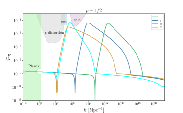
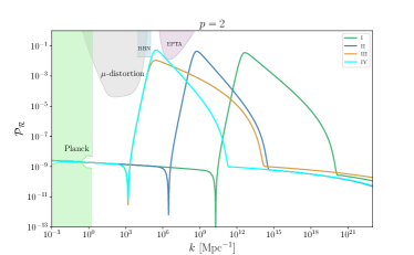
Figure 1: The power spectra produced by the $E$ model for $p=1/2$ (left panel) and $p=2$ (right panel). They are enhanced to $\mathcal{O}(0.01)$ on small scales. The solid colored lines represent the power spectra and the shaded regions are constraints from observations Akrami et al. (2020); Inomata and Nakama (2019); Inomata et al. (2016); Fixsen et al. (1996).

III Non-Gaussianity

Given the two-point function of primordial curvature perturbations, namely, the power spectrum, we know nothing about the interaction of the primordial perturbations, as well as the non-Gaussian feature. So it is necessary to study the higher-point correlations, in which the least order is the three-point function. This could improve our estimation of the abundance of PBHs and the energy density of SIGWs, as the non-Gaussianity may lead to a huge modificationZhang et al. (2021b). The bispectrum $B_{\mathcal{R}}$ is related to the three-point function as Byrnes et al. (2010); Ade et al. (2016)

$$\left\langle\hat{\mathcal{R}}_{\bm{k}_{1}}\hat{\mathcal{R}}_{\bm{k}_{2}}\hat{\mathcal{R}}_{\bm{k}_{3}}\right\rangle=(2\pi)^{3}\delta^{3}\left(\bm{k}_{1}+\bm{k}_{2}+\bm{k}_{3}\right)B_{\mathcal{R}}\left(k_{1},k_{2},k_{3}\right),$$ (14)

where the three-point function $\left\langle\hat{\mathcal{R}}_{\bm{k}_{1}}\hat{\mathcal{R}}_{\bm{k}_{2}}\hat{\mathcal{R}}_{\bm{k}_{3}}\right\rangle$ can be computed using in-in formula Maldacena (2003); Adshead et al. (2009); De Felice and Tsujikawa (2011b)

$$\left\langle\hat{\mathcal{R}}_{\bm{k}_{1}}\hat{\mathcal{R}}_{\bm{k}_{2}}\hat{\mathcal{R}}_{\bm{k}_{3}}\right\rangle\simeq 2\Im\left[\int_{t_{i}}^{t_{e}}dt\left\langle\hat{\mathcal{R}}^{I}_{\bm{k}_{1}}\left(t_{e}\right)\hat{\mathcal{R}}^{I}_{\bm{k}_{2}}\left(t_{e}\right)\hat{\mathcal{R}}^{I}_{\bm{k}_{3}}\left(t_{e}\right)\hat{H}_{I}(t)\right\rangle\right],$$ (15)

where $\hat{\mathcal{R}}^{I}$ is the operator in the interaction picture, $t_{e}$ and $t_{i}$ are the end of inflation and some early time when the perturbations are well within the horizon, respectively. $\Im$ represents the imaginary part of the argument and the interaction Hamiltonian

$$H_{I}=-\int d^{3}x\mathcal{L}_{3}.$$ (16)

The lengthy expressions of cubic Lagrangian $\mathcal{L}_{3}$ and the bispectrum can be found in the appendix A. The non-Gaussianity parameter $f_{\text{NL}}$ is defined as Creminelli et al. (2007); Byrnes et al. (2010)

$$f_{\text{NL}}(k_{1},k_{2},k_{3})=\frac{5}{6}\frac{B_{\mathcal{R}}(k_{1},k_{2},k_{3})}{P_{\mathcal{R}}(k_{1})P_{\mathcal{R}}(k_{2})+P_{\mathcal{R}}(k_{2})P_{\mathcal{R}}(k_{3})+P_{\mathcal{R}}(k_{3})P_{\mathcal{R}}(k_{1})},$$ (17)

where $P_{\mathcal{R}}(k)=\frac{2\pi^{2}}{k^{3}}\mathcal{P}_{\mathcal{R}}(k)$.

With the above formulas, we numerically compute the bispectrum of primordial curvature perturbations and the corresponding non-Gaussianity parameter $f_{\mathrm{NL}}$ defined by (17). One may wonder if our numerical results are accurate in spite of the complexity of the computation. Fortunately, there is a consistency relation given by Maldacena (2003)

$$\frac{12}{5}\lim_{k_{3}\rightarrow 0}f_{\mathrm{NL}}(k_{1},k_{2},k_{3})=1-n_{\mathrm{s}},\quad\text{for}~{}k_{1}=k_{2}.$$ (18)

It was shown that this relation always holds for single field inflation Creminelli and Zaldarriaga (2004), which can be an ideal tool to test our numerical results. We show the spectral index and the non-Gaussianity parameter $f_{\mathrm{NL}}$ in squeezed limit for the parameter set I with $p=1/2$ in Fig. 2. From Fig. 2, the consistency relation (18) holds, which enhances our confidence on the numerical results, more or less. Besides, we also show the non-Gaussianity parameter $f_{\mathrm{NL}}$ in the equilateral limit. From Fig. 2, the non-Gaussianity parameter is small at peak scales though it can be pretty large at the beginning of the USR phase.

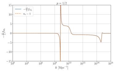
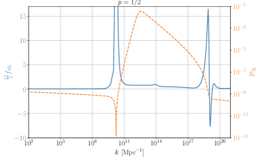
Figure 2: The non-Gaussianity parameter $f_{\mathrm{NL}}$, spectral index $n_{s}-1$ and power spectrum for parameter set I. In the left panel, we show $n_{s}-1$ in the solid line, and the non-Gaussianity parameter $-\frac{12}{5}f_{\mathrm{NL}}$ in squeezed limit for $k_{1}=k_{2}=10^{6}k_{3}=k$ in the dashed line. In the right panel, we show the non-Gaussianity parameter $\frac{12}{5}f_{\mathrm{NL}}$ in equilateral limit for $k_{1}=k_{2}=k_{3}=k$ and the power spectrum in solid and dashed line, respectively.

IV PBHs and SIGWs

Large perturbations will cause gravitational collapse to form PBHs after horizon reentry during radiation domination accompanied by the generation of SIGWs. In this section, we compute the abundance of PBHs and the fractional energy density of SIGWs from the $E$ model. We also consider the effects of non-Gaussianity.

IV.1 PBHs

The mass of PBH at the formation time is $\gamma M_{\mathrm{hor}}$, where $M_{\mathrm{hor}}$ is the horizon mass and $\gamma$ is a numerical factor that depends on the details of gravitational collapse. We choose the factor $\gamma=0.2$ Carr (1975). The current fractional energy density of PBHs with mass $M$ in DM is Carr et al. (2016); Di and Gong (2018)

$$\begin{split}Y_{\text{PBH}}(M)=&\frac{\beta(M)}{3.94\times 10^{-9}}\left(\frac{\gamma}{0.2}\right)^{1/2}\left(\frac{g_{*}}{10.75}\right)^{-1/4}\times\left(\frac{0.12}{\Omega_{\text{DM}}h^{2}}\right)\left(\frac{M}{M_{\odot}}\right)^{-1/2},\end{split}$$ (19)

where $M_{\odot}$ is the solar mass, $g_{*}$ is the effective degrees of freedom at the formation time, $\Omega_{\text{DM}}$ is the current energy density parameter of DM, and $\beta$ is the fractional energy density of PBHs at the formation. In Press-Schechter theory Press and Schechter (1974), the fraction $\beta$ could be regarded as the probability that the density contrast exceeds the threshold

$$\beta=2\int_{\delta_{c}}^{\infty}P(\delta)d\delta,$$ (20)

where $P(\delta)$ is the probability distribution function (PDF) of density contrast $\delta$, and $\delta_{c}$ is the threshold for the formation of PBHs. For Gaussian statistic

$$\beta^{G}(M)\approx\sqrt{\frac{2}{\pi}}\frac{\sigma(M)}{\delta_{c}}\exp\left(-\frac{\delta_{c}^{2}}{2\sigma^{2}(M)}\right),$$ (21)

where $\sigma^{2}$ is the variance of $\delta$ smoothed on the horizon scales $R=1/(aH)$,

$$\sigma^{2}(M)=\left(\frac{4}{9}\right)^{2}\int\frac{dk}{k}\widetilde{\text{W}}^{2}(kR)(kR)^{4}\mathcal{P}_{\mathcal{R}}(k),$$ (22)

We choose a Gaussian window function $\widetilde{\mathrm{W}}(x)=\mathrm{e}^{-x^{2}/2}$. The effective degree of freedom is $g_{*}=107.5$ for $T>300$ GeV and $g_{*}=10.75$ for $0.5\text{~{}MeV}<T<300\text{~{}GeV}$. We take the observational value $\Omega_{\text{DM}}h^{2}=0.12$ Aghanim et al. (2020) and threshold $\delta_{c}=0.44$ Harada et al. (2013); Tada and Yokoyama (2019); Escrivà et al. (2020) in the calculation of PBH abundance. The relation between the PBH mass $M$ and the scale $k$ is Di and Gong (2018)

$$M(k)=3.68\left(\frac{\gamma}{0.2}\right)\left(\frac{g_{*}}{10.75}\right)^{-1/6}\left(\frac{k}{10^{6}\ \text{Mpc}^{-1}}\right)^{-2}M_{\odot}.$$ (23)

With Eqs. (19), (21), (23) and the power spectrum obtained in Sec. II, we compute the PBH DM abundance with Gaussian approximation, $Y^{G}_{\mathrm{PBH}}$, and the results are shown in Table 2 and Fig. 3. For parameter set I, the $E$ model with both $p=1/2$ and $p=2$ produces PBHs with mass around $M_{\mathrm{PBH}}\sim 10^{-13}-10^{-12}M_{\odot}$. The PBH abundance at the peak is $Y^{G}_{\mathrm{PBH}}\simeq 0.969$ for $p=1/2$ and $Y^{G}_{\mathrm{PBH}}\simeq 0.79$ for $p=2$, respectively. In this mass range, PBHs can be all DM. For parameter set II, our model produces PBHs with the mass range $M_{\mathrm{PBH}}\sim 10^{-6}-10^{-5}M_{\odot}$ for both $p=1/2$ and $p=2$, the abundance of PBHs are $Y^{G}_{\mathrm{PBH}}\simeq 0.027$ and $Y^{G}_{\mathrm{PBH}}\simeq 0.021$, respectively. PBHs in this range can explain the ultrashort-timescale microlensing events in the OGLE data Mróz et al. (2017); Niikura et al. (2019a). For parameter set IV, the models of both $p=1/2$ and $p=2$ produce PBHs with mass around $M_{\mathrm{PBH}}\sim 30M_{\odot}$. These PBHs can explain the LIGO events.

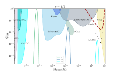
Figure 3: The PBH DM abundance $Y^{G}_{\mathrm{PBH}}$ produced by the $E$ model with Gaussian statistic perturbation. The left panel shows the results for $p=1/2$, and the right panel shows the results for $p=2$. The green-cyan shaded region presents the allowed PBH abundance from the ultrashort-timescale microlensing events in the OGLE data Mróz et al. (2017); Niikura et al. (2019a). The other shaded regions, the dashed line, and the dotted line are the constraints on PBHs abundance from various observations Sato-Polito et al. (2019); Carr et al. (2010); Laha (2019); Dasgupta et al. (2020); Niikura et al. (2019b); Griest et al. (2013); Tisserand et al. (2007); Ali-Haïmoud et al. (2017); Raidal et al. (2017); Ali-Haïmoud and Kamionkowski (2017); Poulin et al. (2017); Wang et al. (2019); Laha et al. (2020, 2021).

We discuss the role that the non-Gaussianity plays in the formation of PBHs qualitatively, and then we present the numerical result. From the viewpoint of statistics, a non-vanishing three-point function that relates to the skewness of a PDF implies a non-Gaussian tail, as the schematic shown in Fig. 4 for illustration. A positive three-point function, $\langle\delta\delta\delta\rangle>0$, corresponds to a right-tailed PDF, so the probability of obtaining perturbations with $\nu=\delta/\sigma\gg 1$ becomes larger relative to a Gaussian PDF, and vice versa. The formation of PBHs is a rare event, mainly attributed to the large perturbations with $\nu\geq\nu_{c}=\delta_{c}/\sigma\gg 1$. The abundance of PBHs $\beta$ at the formation corresponds to the area below the PDF with $\nu\geq\nu_{c}$ according to Eq. (4). This is sensitive to the non-Gaussian tail. In addition, from Fig. 4, we see that the Gaussian-predicted PBH abundance $\beta^{G}$ is enhanced/suppressed if the three-point function is positive/negative.

Then we discuss the effect of non-Gaussianity on the PBH abundance, quantitatively. The mass fraction $\beta$ with non-Gaussian corrected Franciolini et al. (2018); Riccardi et al. (2021)

$$\beta=\text{e}^{\Delta_{3}}\beta^{G},$$ (24)

where the 3rd cumulant $\Delta_{3}$

$$\Delta_{3}=\frac{1}{3!}\left(\frac{\delta_{c}}{\sigma}\right)^{2}\mathcal{S}_{3}\delta_{c},$$ (25)

with

$$\mathcal{S}_{3}=\frac{\left\langle\delta(\bm{x})\delta(\bm{x})\delta(\bm{x})\right\rangle}{\sigma^{4}}.$$ (26)

Since the mass of PBHs is almost monochromatic, we only consider the correction from peak-scale perturbation Zhang et al. (2021b)

$$\Delta_{3}\approx 23\frac{\delta^{3}_{c}}{\mathcal{P}_{\mathcal{R}}(k_{\text{peak}})}f_{\mathrm{NL}}(k_{\text{peak}},k_{\text{peak}},k_{\text{peak}}).$$ (27)

We compute $f_{\mathrm{NL}}(k_{\text{peak}},k_{\text{peak}},k_{\text{peak}})$ numerically and show the results in Table. 2. The non-Gaussianity parameter $f_{\mathrm{NL}}(k_{\text{peak}},k_{\text{peak}},k_{\text{peak}})$ is about $\mathcal{O}(0.1)$, and $\Delta_{3}\sim\mathcal{O}(10)$, which means the PBH abundance is highly underestimated using just Gaussian approximation. There are more PBHs due to the right-tailed PDF, which is consistent with our above qualitative discussion.

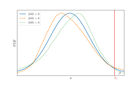
Figure 4: The PDF of $\delta$ for $\langle\delta\delta\delta\rangle=0$ (solid line), $\langle\delta\delta\delta\rangle>0$ (dashed line), and $\langle\delta\delta\delta\rangle<0$ (dotted line). The red vertical line represents the threshold for PBH formation. The area below the PDF with $\nu\geq\nu_{c}$ represents the PBH abundance at the formation time.

IV.2 SIGWs

The energy density parameter of SIGWs per logarithmic interval of ${k}$ can be expressed as following Kohri and Terada (2018); Espinosa et al. (2018)

$$\Omega_{\mathrm{GW}}\left(k\right)=\frac{1}{24}\left(\frac{k}{a(\tau)H(\tau)}\right)^{2}\overline{\mathcal{P}_{h}\left(k,\tau\right)},$$ (28)

where the power spectrum of SIGWs averaged for several wavelengths $\overline{\mathcal{P}_{h}}$

$$\overline{\mathcal{P}_{h}\left(k,\tau\right)}=4\int^{\infty}_{0}dv\int^{1+v}_{\left|1-v\right|}du\left(\frac{4v^{2}-\left(1+v^{2}-u^{2}\right)^{2}}{4vu}\right)^{2}\overline{I^{2}_{\mathrm{RD}}\left(u,v,x\right)}\mathcal{P}_{\mathcal{R}}\left(uk\right)\mathcal{P}_{\mathcal{R}}\left(vk\right),$$ (29)

with $x=k\tau$ and ${I^{2}_{\mathrm{RD}}\left(u,v,x\rightarrow\infty\right)}$ is

$$\begin{split}\overline{I_{\mathrm{RD}}^{2}(v,u,x\rightarrow\infty)}=&\frac{1}{2x^{2}}\left(\frac{3(u^{2}+v^{2}-3)}{4u^{3}v^{3}}\right)^{2}\left\{\left(-4uv+(u^{2}+v^{2}-3)\log\left|\frac{3-(u+v)^{2}}{3-(u-v)^{2}}\right|\right)^{2}\right.\\ &\left.\vphantom{\log\left|\frac{3-(u+v)^{2}}{3-(u-v)^{2}}\right|^{2}}\qquad\qquad\qquad\qquad\qquad+\pi^{2}(u^{2}+v^{2}-3)^{2}\Theta\left(v+u-\sqrt{3}\right)\right\}.\end{split}$$ (30)

The fractional energy density of SIGWs today $\Omega_{\mathrm{GW},0}$ Espinosa et al. (2018)

$$\Omega_{\mathrm{GW},0}\left(k\right)=\Omega_{\mathrm{GW}}\left(k\right)\frac{\Omega_{r,0}}{\Omega_{r}\left(\tau\right)},$$ (31)

where $\Omega_{r,0}$ is the current fractional energy density of radiation. We choose $\Omega_{r}=1$ during the radiation domination.

With the power spectrum obtained in Sec. II, we compute the fractional energy density of SIGWs from the $E$ model, the results are shown in Table. 2 and Fig. 5. The SIGWs with peak frequency being milli-Hertz can be detected by TianQin, Taiji, and LISA. The SIGWs with peak frequency $f_{c}\sim 10^{-6}$Hz can be tested by SKA. For parameter set IV, the SIGWs can be observed by both SKA and EPTA. With parameter set III, the $E$ model produces a broad power spectrum, and the corresponding spectrum of SIGWs is flatter than the others. The energy density of SIGWs lies within the $2\sigma$ region of the NANOGrav signal De Luca et al. (2021b); Vaskonen and Veermäe (2021); Kohri and Terada (2021); Domènech and Pi (2022); Vagnozzi (2021).

To estimate the contribution from non-Gaussianity, we use nonlinear coupling constant $f_{\text{NL}}$ defined by Verde et al. (2000); Komatsu and Spergel (2001)

$$\mathcal{R}(\bm{x})=\mathcal{R}^{G}(\bm{x})+\frac{3}{5}f_{\text{NL}}(\mathcal{R}^{G}(\bm{x})^{2}-\langle\mathcal{R}^{G}(\bm{x})^{2}\rangle),$$ (32)

where $\mathcal{R}^{G}$ is the linear Gaussian part of the curvature perturbations. Then the power spectrum of curvature perturbations taking into account the non-Gaussianity can be expressed as

$$\mathcal{P}_{\mathcal{R}}(k)=\mathcal{P}^{G}_{\mathcal{R}}(k)+\mathcal{P}^{NG}_{\mathcal{R}}(k),$$ (33)

where

$$\mathcal{P}^{NG}_{\mathcal{R}}(k)=\left(\frac{3}{5}\right)^{2}\frac{k^{3}}{2\pi}f^{2}_{\mathrm{NL}}\int d^{3}\bm{p}\frac{\mathcal{P}^{G}_{\mathcal{R}}(p)}{p^{3}}\frac{\mathcal{P}^{G}_{\mathcal{R}}(|\bm{k}-\bm{p}|)}{|\bm{k}-\bm{p}|^{3}}.$$ (34)

The non-Gaussian contribution to the energy density of SIGWs is insignificant unless $\left(\frac{3}{5}\right)^{2}f^{2}_{\text{NL}}\mathcal{P}^{G}_{\mathcal{R}}\gtrsim 1$ Cai et al. (2019). From our results, $f_{\text{NL}}\sim\mathcal{O}(0.1)$, and $\mathcal{P}^{G}_{\mathcal{R}}\sim\mathcal{O}(0.01)$ at peak scales, so the effects of non-Gaussianity on SIGWs is neglegible.

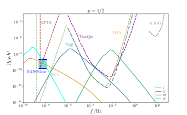
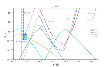
Figure 5: The SIGWs generated by the $E$ model with $p=1/2$ (left panel) and $p=2$ (right panel). The solid curves represent the energy density of SIGWs. The fuchsia dashed curve shows the EPTA limit Ferdman et al. (2010); Hobbs et al. (2010); McLaughlin (2013); Hobbs (2013) , the SKA limit Moore et al. (2015) is shown in the lime dashed curve, the purple dashed curve in the middle denotes the TianQin limit Luo et al. (2016), the dark cyan dotted-dashed curve shows the Taiji limit Hu and Wu (2017), the orange dashed curve denotes the LISA limit Amaro-Seoane et al. (2017), and the aLIGO limit Harry (2010); Aasi et al. (2015) shown in the gray dashed curve.

V Conclusion

The higher-order curvature correction of gravity may play an important role in the early Universe. In this paper, we use an $E$ model potential to drive inflation with the Gauss-Bonnet term. In this model, the power spectrum can not only satisfy the constraints from CMB on large scales, but also reach $\mathcal{O}(0.01)$ on small scales due to Gauss-Bonnet coupling. The large perturbations cause gravitational collapse to form PBHs, accompanied by the generation of SIGWs after horizon reentry during the radiation domination. By tuning the model parameters, the power spectrum can be enhanced at various scales and thus we can obtain PBHs with different mass ranges. The PBHs with mass range $\mathcal{O}(10^{-13})-\mathcal{O}(10^{-12})M_{\odot}$ makes up almost all DM, and the corresponding SIGWs is observable by space-based GWs observatories, like TianQin, Taiji and LISA. The abundance of PBHs with mass in the range $\mathcal{O}(10^{-6})-\mathcal{O}(10^{-5})M_{\odot}$ can be $Y^{G}_{\mathrm{PBH}}\sim\mathcal{O}(0.02)$. These PBHs could explain the ultrashort-timescale microlensing events in the OGLE data, and the SIGWs can be tested by SKA. With the parameter set IV, the mass of PBHs is around $\sim 30M_{\odot}$. These PBHs could explain the LIGO-Virgo events. Meanwhile, the Nanohertz SIGWs are observable by SKA and EPTA. With parameter set III, we get a broad peak in the power spectrum, and the corresponding SIGWs can explain the signal hinted by NANOGrav.

We also consider the effect of non-Gaussianity on the abundance of PBHs and the fractional energy density of SIGWs. We find that more PBHs can be produced. The abundance of PBHs receives a significant enhancement due to the right-tailed PDF. However, the fractional energy density of SIGWs is insensitive to non-Gaussianity and remains almost unaffected.

Appendix A The Cubic Action And The Bispectrum

The cubic action used to compute the bispectrum is De Felice and Tsujikawa (2011a)

$$\begin{split}S_{3}=&\int dtd^{3}x\left\{a^{3}\mathcal{C}_{1}\mathcal{R}\dot{\mathcal{R}}^{2}+a\mathcal{C}_{2}\mathcal{R}(\partial\mathcal{R})^{2}+a^{3}\mathcal{C}_{3}\dot{\mathcal{R}}^{3}+a^{3}\mathcal{C}_{4}\dot{\mathcal{R}}\left(\partial_{i}\mathcal{R}\right)\left(\partial_{i}\chi\right)\right.\\ &+a^{3}\mathcal{C}_{5}\partial^{2}\mathcal{R}(\partial\chi)^{2}+a\mathcal{C}_{6}\dot{\mathcal{R}}^{2}\partial^{2}\mathcal{R}+\left(\mathcal{C}_{7}/a\right)\left[\partial^{2}\mathcal{R}(\partial\mathcal{R})^{2}-\mathcal{R}\partial_{i}\partial_{j}\left(\partial_{i}\mathcal{R}\right)\left(\partial_{j}\mathcal{R}\right)\right]\\ &\left.+a\mathcal{C}_{8}\left[\partial^{2}\mathcal{R}\partial_{i}\mathcal{R}\partial_{i}\chi-\mathcal{R}\partial_{i}\partial_{j}\left(\partial_{i}\mathcal{R}\right)\left(\partial_{j}\chi\right)\right]+\left.\mathcal{F}_{1}\frac{\delta\mathcal{L}_{2}}{\delta\mathcal{R}}\right|_{1}\right\}\end{split}$$ (35)

where $\mathcal{L}_{2}$ is the quadratic Lagrangian and $\partial^{2}\mathcal{\chi}=Q\dot{\mathcal{R}}$, and

$$\begin{split}\mathcal{F}_{1}=&\frac{A_{5}}{w_{1}^{2}}\left\{\left(\partial_{i}\mathcal{R}\right)\left(\partial_{i}\chi\right)-\partial^{-2}\partial_{i}\partial_{j}\left[\left(\partial_{i}\mathcal{R}\right)\left(\partial_{j}\chi\right)\right]\right\}\\ &+q_{1}\mathcal{R}\dot{\mathcal{R}}+\frac{A_{7}-2A_{5}L_{1}}{4w_{1}a^{2}}\left\{(\partial\mathcal{R})^{2}-\partial^{-2}\partial_{i}\partial_{j}\left[\left(\partial_{i}\mathcal{R}\right)\left(\partial_{j}\mathcal{R}\right)\right]\right\}.\end{split}$$ (36)

The expressions of $\mathcal{C}_{1}-\mathcal{C}_{8}$ are as follows

$$\begin{split}&w_{1}=1-\frac{1}{2}\xi_{1},\ \ w_{2}=2H(1-\frac{3}{4}\xi_{1}),\\ &w_{3}=-3H^{2}(3-\epsilon_{1}-\frac{11}{4}\xi_{1}+\frac{1}{4}\epsilon_{1}\xi_{1}-\frac{1}{4}\xi_{1}\xi_{2}),\\ &w_{4}=1-\frac{1}{2}(\epsilon_{1}\xi_{1}+\xi_{1}\xi_{2}),\ \ L_{1}=\frac{2w_{1}}{w_{2}};\end{split}$$ (37)

$$\begin{split}&a_{1}=H^{2}(3-\epsilon_{1}-\frac{19}{4}\xi_{1}+\frac{1}{4}\epsilon_{1}\xi_{1}-\frac{1}{4}\xi_{1}\xi_{2}),\ \ a_{2}=w_{3},\\ &a_{3}=-3H(2-3\xi_{1}),\ \ a_{4}=-\xi_{1},\ \ a_{5}=H(2-3\xi_{1}),\\ &a_{6}=-w_{2},\ \ a_{7}=9w_{2},\ \ a_{8}=\frac{\xi_{1}}{H},\ \ a_{9}=-\frac{1-3\xi_{1}/2}{2},\\ &a_{10}=\frac{\xi_{1}}{2H},\ \ a_{11}=-w_{2},\ \ a_{12}=4a_{9},\ \ a_{13}=-2w_{1},\\ &a_{14}=-w_{1},\ \ a_{15}=-6a_{9};\end{split}$$ (38)

$$b_{1}=\frac{1}{2}a_{8},\ \ b_{2}=w_{4},\ \ b_{3}=-9w_{1};$$ (39)

$$c_{1}=c_{3}=-a_{13},\ \ c_{2}=-a_{10};$$ (40)

$$d_{1}=-\frac{\xi_{1}}{4H},\ \ d_{2}=\frac{3}{2}w_{1},\ \ d_{3}=-2w_{1};$$ (41)

$$\begin{split}&A_{1}=b_{1}+L_{1}a_{15}+L_{1}^{2}a_{3}+L_{1}^{3}a_{1},\ \ A_{2}=L_{1}\left(L_{1}a_{4}+a_{8}\right),\\ &A_{3}=c_{2}+L_{1}a_{12}+L_{1}^{2}a_{5},\ \ A_{4}=b_{3}+L_{1}a_{7}+L_{1}^{2}a_{2},\\ &A_{5}=L_{1}a_{9}+d_{1},\ \ A_{6}=d_{2},\ \ A_{7}=L_{1}a_{10},\\ &A_{8}=b_{2}+a_{13}\dot{L}_{1}/2+L_{1}\left(\dot{a}_{13}+Ha_{13}\right)/2,\ \ A_{9}=d_{3};\end{split}$$ (42)

$$\begin{split}&q_{1}=-\frac{L_{1}}{c^{2}_{s}},\\ &q_{2}=-\frac{4A_{6}L_{1}}{w_{1}}-a^{2}\frac{d}{dt}\left(\frac{A_{7}-2A_{5}L_{1}}{a^{2}w_{1}}\right)-\frac{2A_{9}L_{1}}{w_{1}},\\ &q_{3}=A_{6}L_{1}^{2}-\frac{a}{3}\frac{d}{dt}\left(\frac{A_{5}L_{1}^{2}-A_{7}L_{1}}{a}\right)+\frac{2}{3}A_{9}L_{1}^{2}.\end{split}$$ (43)

$$\begin{split}&\mathcal{C}_{1}=A_{4}+q_{1}(\dot{Q}+3HQ)-Q\dot{q}_{1},\ \ \mathcal{C}_{2}=A_{8}+\frac{1}{a}\frac{d}{dt}\left(aL_{1}Q\right),\\ &\mathcal{C}_{3}=A_{1}+A_{3}\frac{Q}{w_{1}}-q_{1}Q,\\ &\mathcal{C}_{4}=\frac{Q}{w_{1}}\left[\frac{1}{w_{1}}\left(A_{6}+A_{9}\right)-w_{1}\frac{d}{dt}\left(\frac{A_{5}}{w_{1}^{2}}\right)+\frac{3HA_{5}}{w_{1}}\right],\\ &\mathcal{C}_{5}=\frac{1}{2}\left[\frac{A_{6}}{w_{1}^{2}}-\frac{d}{dt}\left(\frac{A_{5}}{w_{1}^{2}}\right)+\frac{3HA_{5}}{w_{1}^{2}}\right],\\ &\mathcal{C}_{6}=A_{2}-A_{3}L_{1},\ \ \mathcal{C}_{7}=q_{3}-\frac{Qc_{s}^{2}}{2w_{1}}\left(A_{7}-2A_{5}L_{1}\right),\ \ \mathcal{C}_{8}=\frac{q_{2}}{2}-\frac{2c_{s}^{2}A_{5}Q}{w_{1}^{2}}.\end{split}$$ (44)

With the above expressions of the coefficients, the explicit form of bispectrum $B_{\mathcal{R}}$

$$B_{\mathcal{R}}(k_{1},k_{2},k_{3})=\mathcal{R}_{k_{1}}(t_{e})\mathcal{R}_{k_{2}}(t_{e})\mathcal{R}_{k_{3}}(t_{e})\sum_{i=1}^{10}\mathcal{B}^{i}_{\mathcal{R}}(k_{1},k_{2},k_{3}),$$ (45)

where

$$\mathcal{B}^{1}_{\mathcal{R}}(k_{1},k_{2},k_{3})=-4\Im\int^{t_{e}}_{t_{i}}dta^{3}\mathcal{C}_{1}\left(\mathcal{R}^{*}_{k_{1}}(t)\dot{\mathcal{R}^{*}}_{k_{2}}(t)\dot{\mathcal{R}^{*}}_{k_{3}}(t)+\text{perm}\right),$$ (46)

$$\mathcal{B}^{2}_{\mathcal{R}}(k_{1},k_{2},k_{3})=4\Im\int^{t_{e}}_{t_{i}}dta\mathcal{C}_{2}\left[\left(\bm{k}_{1}\cdot\bm{k}_{2}+\bm{k}_{1}\cdot\bm{k}_{3}+\bm{k}_{2}\cdot\bm{k}_{3}\right)\mathcal{R}^{*}_{k_{1}}(t)\mathcal{R}^{*}_{k_{2}}(t)\mathcal{R}^{*}_{k_{3}}(t)\right],$$ (47)

$$\mathcal{B}^{3}_{\mathcal{R}}(k_{1},k_{2},k_{3})=-12\Im\int^{t_{e}}_{t_{i}}dta^{3}\mathcal{C}_{3}\dot{\mathcal{R}^{*}}_{k_{1}}(t)\dot{\mathcal{R}^{*}}_{k_{2}}(t)\dot{\mathcal{R}^{*}}_{k_{3}}(t),$$ (48)

$$\mathcal{B}^{4}_{\mathcal{R}}(k_{1},k_{2},k_{3})=-2\Im\int^{t_{e}}_{t_{i}}dta^{3}\mathcal{C}_{4}Q\left[\left(\frac{\bm{k}_{1}\cdot\bm{k}_{2}}{k^{2}_{2}}+\frac{\bm{k}_{1}\cdot\bm{k}_{3}}{k^{2}_{3}}\right)\mathcal{R}^{*}_{k_{1}}(t)\dot{\mathcal{R}^{*}}_{k_{2}}(t)\dot{\mathcal{R}^{*}}_{k_{3}}(t)+\text{perm}\right],$$ (49)

$$\mathcal{B}^{5}_{\mathcal{R}}(k_{1},k_{2},k_{3})=-4\Im\int^{t_{e}}_{t_{i}}dta^{3}\mathcal{C}_{5}Q^{2}\left[\frac{k^{2}_{1}\bm{k}_{2}\cdot\bm{k}_{3}}{k^{2}_{2}k^{2}_{3}}\mathcal{R}^{*}_{k_{1}}(t)\dot{\mathcal{R}^{*}}_{k_{2}}(t)\dot{\mathcal{R}^{*}}_{k_{3}}(t)+\text{perm}\right],$$ (50)

$$\mathcal{B}^{6}_{\mathcal{R}}(k_{1},k_{2},k_{3})=4\Im\int^{t_{e}}_{t_{i}}dta\mathcal{C}_{6}\left[k^{2}_{1}\mathcal{R}^{*}_{k_{1}}(t)\dot{\mathcal{R}^{*}}_{k_{2}}(t)\dot{\mathcal{R}^{*}}_{k_{3}}(t)+\text{perm}\right],$$ (51)

$$\mathcal{B}^{7}_{\mathcal{R}}(k_{1},k_{2},k_{3})=-4\Im\int^{t_{e}}_{t_{i}}dt\mathcal{C}_{7}/a\left[\left(k^{2}_{1}\bm{k}_{2}\cdot\bm{k}_{3}+k^{2}_{2}\bm{k}_{1}\cdot\bm{k}_{3}+k^{2}_{3}\bm{k}_{1}\cdot\bm{k}_{2}\right)\mathcal{R}^{*}_{k_{1}}(t)\mathcal{R}^{*}_{k_{2}}(t)\mathcal{R}^{*}_{k_{3}}(t)\right],$$ (52)

$$\begin{split}\mathcal{B}^{8}_{\mathcal{R}}(k_{1},k_{2},k_{3})=2\Im\int^{t_{e}}_{t_{i}}dt\mathcal{C}_{7}/a&\left[\left(k^{2}_{2}\bm{k}_{2}\cdot\bm{k}_{3}+k^{2}_{3}\bm{k}_{3}\cdot\bm{k}_{2}+k^{2}_{1}\bm{k}_{1}\cdot\bm{k}_{2}+k^{2}_{1}\bm{k}_{1}\cdot\bm{k}_{3}\right.\right.\\ &\left.\left.+k^{2}_{2}\bm{k}_{2}\cdot\bm{k}_{1}+k^{2}_{3}\bm{k}_{3}\cdot\bm{k}_{1}\right)\mathcal{R}^{*}_{k_{1}}(t)\mathcal{R}^{*}_{k_{2}}(t)\mathcal{R}^{*}_{k_{3}}(t)\right],\end{split}$$ (53)

$$\mathcal{B}^{9}_{\mathcal{R}}(k_{1},k_{2},k_{3})=2\Im\int^{t_{e}}_{t_{i}}dta\mathcal{C}_{8}Q\left[\left(\frac{k^{2}_{1}\bm{k}_{2}\cdot\bm{k}_{3}}{k^{2}_{3}}+\frac{k^{2}_{2}\bm{k}_{1}\cdot\bm{k}_{3}}{k^{2}_{3}}\right)\mathcal{R}^{*}_{k_{1}}(t)\mathcal{R}^{*}_{k_{2}}(t)\dot{\mathcal{R}^{*}}_{k_{3}}(t)+\text{perm}\right],$$ (54)

$$\mathcal{B}^{10}_{\mathcal{R}}(k_{1},k_{2},k_{3})=-2\Im\int^{t_{e}}_{t_{i}}dta\mathcal{C}_{8}Q\left[\left(\frac{k^{2}_{2}\bm{k}_{2}\cdot\bm{k}_{3}}{k^{2}_{3}}+\frac{k^{2}_{1}\bm{k}_{1}\cdot\bm{k}_{3}}{k^{2}_{3}}\right)\mathcal{R}^{*}_{k_{1}}(t)\mathcal{R}^{*}_{k_{2}}(t)\dot{\mathcal{R}^{*}}_{k_{3}}(t)+\text{perm}\right].$$ (55)

The contribution of the last term in Eq. (35) is negligible relative to those coming from other terms, as in Refs. De Felice and Tsujikawa (2011b); Arroja and Tanaka (2011); Rigopoulos (2011), we neglect this term when computing the bispectrum.

References

- Carr and Hawking (1974) B. J. Carr and S. Hawking, Black holes in the early Universe, Mon. Not. R. Astron. Soc. 168, 399 (1974).
- Hawking (1971) S. Hawking, Gravitationally collapsed objects of very low mass, Mon. Not. R. Astron. Soc. 152, 75 (1971).
- Abbott et al. (2016a) B. P. Abbott et al. (LIGO Scientific and Virgo Collaborations), GW151226: Observation of Gravitational Waves from a 22-Solar-Mass Binary Black Hole Coalescence, Phys. Rev. Lett. 116, 241103 (2016a), arXiv:1606.04855 .
- Abbott et al. (2016b) B. P. Abbott et al. (LIGO Scientific and Virgo Collaborations), Observation of Gravitational Waves from a Binary Black Hole Merger, Phys. Rev. Lett. 116, 061102 (2016b), arXiv:1602.03837 .
- Abbott et al. (2017a) B. P. Abbott et al. (LIGO Scientific and Virgo Collaborations), GW170608: Observation of a 19-solar-mass Binary Black Hole Coalescence, Astrophys. J. Lett. 851, L35 (2017a), arXiv:1711.05578 .
- Abbott et al. (2017b) B. P. Abbott et al. (LIGO Scientific and Virgo Collaborations), GW170817: Observation of Gravitational Waves from a Binary Neutron Star Inspiral, Phys. Rev. Lett. 119, 161101 (2017b), arXiv:1710.05832 .
- Abbott et al. (2017c) B. P. Abbott et al. (LIGO Scientific and Virgo Collaborations), GW170814: A Three-Detector Observation of Gravitational Waves from a Binary Black Hole Coalescence, Phys. Rev. Lett. 119, 141101 (2017c), arXiv:1709.09660 .
- Abbott et al. (2017d) B. P. Abbott et al. (LIGO Scientific and Virgo Collaborations), GW170104: Observation of a 50-Solar-Mass Binary Black Hole Coalescence at Redshift 0.2, Phys. Rev. Lett. 118, 221101 (2017d), [Erratum: Phys. Rev. Lett.121,no.12,129901(2018)], arXiv:1706.01812 .
- Abbott et al. (2019) B. P. Abbott et al. (LIGO Scientific and Virgo Collaborations), GWTC-1: A Gravitational-Wave Transient Catalog of Compact Binary Mergers Observed by LIGO and Virgo during the First and Second Observing Runs, Phys. Rev. X9, 031040 (2019), arXiv:1811.12907 .
- Abbott et al. (2020a) R. Abbott et al. (LIGO Scientific and Virgo Collaborations), GW190814: Gravitational Waves from the Coalescence of a 23 Solar Mass Black Hole with a 2.6 Solar Mass Compact Object, Astrophys. J. Lett. 896, L44 (2020a), arXiv:2006.12611 .
- Abbott et al. (2020b) B. Abbott et al. (LIGO Scientific and Virgo Collaborations), GW190425: Observation of a Compact Binary Coalescence with Total Mass , Astrophys. J. Lett. 892, L3 (2020b), arXiv:2001.01761 .
- Abbott et al. (2020c) R. Abbott et al. (LIGO Scientific and Virgo Collaborations), GW190412: Observation of a Binary-Black-Hole Coalescence with Asymmetric Masses, Phys. Rev. D 102, 043015 (2020c), arXiv:2004.08342 .
- Bird et al. (2016) S. Bird, I. Cholis, J. B. Muñoz, Y. Ali-Haïmoud, M. Kamionkowski, E. D. Kovetz, A. Raccanelli, and A. G. Riess, Did LIGO detect dark matter?, Phys. Rev. Lett. 116, 201301 (2016), arXiv:1603.00464 .
- Sasaki et al. (2016) M. Sasaki, T. Suyama, T. Tanaka, and S. Yokoyama, Primordial Black Hole Scenario for the Gravitational-Wave Event GW150914, Phys. Rev. Lett. 117, 061101 (2016), [Erratum: Phys.Rev.Lett. 121, 059901 (2018)], arXiv:1603.08338 .
- Takhistov et al. (2021) V. Takhistov, G. M. Fuller, and A. Kusenko, Test for the Origin of Solar Mass Black Holes, Phys. Rev. Lett. 126, 071101 (2021), arXiv:2008.12780 .
- De Luca et al. (2021a) V. De Luca, V. Desjacques, G. Franciolini, P. Pani, and A. Riotto, GW190521 Mass Gap Event and the Primordial Black Hole Scenario, Phys. Rev. Lett. 126, 051101 (2021a), arXiv:2009.01728 .
- Abbott et al. (2021) R. Abbott et al. (LIGO Scientific and Virgo Collaborations), GWTC-2: Compact Binary Coalescences Observed by LIGO and Virgo During the First Half of the Third Observing Run, Phys. Rev. X 11, 021053 (2021), arXiv:2010.14527 .
- Saito and Yokoyama (2009) R. Saito and J. Yokoyama, Gravitational wave background as a probe of the primordial black hole abundance, Phys. Rev. Lett. 102, 161101 (2009), [Erratum: Phys.Rev.Lett. 107, 069901 (2011)], arXiv:0812.4339 .
- Orlofsky et al. (2017) N. Orlofsky, A. Pierce, and J. D. Wells, Inflationary theory and pulsar timing investigations of primordial black holes and gravitational waves, Phys. Rev. D 95, 063518 (2017), arXiv:1612.05279 .
- Nakama et al. (2017) T. Nakama, J. Silk, and M. Kamionkowski, Stochastic gravitational waves associated with the formation of primordial black holes, Phys. Rev. D 95, 043511 (2017), arXiv:1612.06264 .
- Wang et al. (2018) S. Wang, Y.-F. Wang, Q.-G. Huang, and T. G. F. Li, Constraints on the Primordial Black Hole Abundance from the First Advanced LIGO Observation Run Using the Stochastic Gravitational-Wave Background, Phys. Rev. Lett. 120, 191102 (2018), arXiv:1610.08725 .
- Cai et al. (2019) R.-g. Cai, S. Pi, and M. Sasaki, Gravitational Waves Induced by non-Gaussian Scalar Perturbations, Phys. Rev. Lett. 122, 201101 (2019), arXiv:1810.11000 .
- Kohri and Terada (2018) K. Kohri and T. Terada, Semianalytic calculation of gravitational wave spectrum nonlinearly induced from primordial curvature perturbations, Phys. Rev. D 97, 123532 (2018), arXiv:1804.08577 .
- Espinosa et al. (2018) J. R. Espinosa, D. Racco, and A. Riotto, A Cosmological Signature of the SM Higgs Instability: Gravitational Waves, J. Cosmol. Astropart. Phys. 09 (2018) 012, arXiv:1804.07732 .
- Kuroyanagi et al. (2018) S. Kuroyanagi, T. Chiba, and T. Takahashi, Probing the Universe through the Stochastic Gravitational Wave Background, J. Cosmol. Astropart. Phys. 11 (2018) 038, arXiv:1807.00786 .
- Domènech (2020) G. Domènech, Induced gravitational waves in a general cosmological background, Int. J. Mod. Phys. D 29, 2050028 (2020), arXiv:1912.05583 .
- Fumagalli et al. (2021) J. Fumagalli, S. Renaux-Petel, and L. T. Witkowski, Oscillations in the stochastic gravitational wave background from sharp features and particle production during inflation, J. Cosmol. Astropart. Phys. 08 (2021) 030, arXiv:2012.02761 .
- Domènech et al. (2020) G. Domènech, S. Pi, and M. Sasaki, Induced gravitational waves as a probe of thermal history of the universe, J. Cosmol. Astropart. Phys. 08 (2020) 017, arXiv:2005.12314 .
- Domènech (2021) G. Domènech, Scalar Induced Gravitational Waves Review, Universe 7, 398 (2021), arXiv:2109.01398 .
- Wang and Kohri (2021) S. Wang and K. Kohri, Probing Primordial Black Holes with Angular Power Spectrum for Anisotropies in Stochastic Gravitational-Wave Background, arXiv:2107.01935 .
- Adshead et al. (2021) P. Adshead, K. D. Lozanov, and Z. J. Weiner, Non-Gaussianity and the induced gravitational wave background, J. Cosmol. Astropart. Phys. 10 (2021) 080, arXiv:2105.01659 .
- Ahmed et al. (2021) W. Ahmed, M. Junaid, and U. Zubair, Primordial Black Holes and Gravitational Waves in Hybrid Inflation with Chaotic Potentials, arXiv:2109.14838 .
- Akrami et al. (2020) Y. Akrami et al. (Planck), Planck 2018 results. X. Constraints on inflation, Astron. Astrophys. 641, A10 (2020), arXiv:1807.06211 .
- Motohashi and Hu (2017) H. Motohashi and W. Hu, Primordial Black Holes and Slow-Roll Violation, Phys. Rev. D 96, 063503 (2017), arXiv:1706.06784 .
- Sato-Polito et al. (2019) G. Sato-Polito, E. D. Kovetz, and M. Kamionkowski, Constraints on the primordial curvature power spectrum from primordial black holes, Phys. Rev. D 100, 063521 (2019), arXiv:1904.10971 .
- Lu et al. (2019) Y. Lu, Y. Gong, Z. Yi, and F. Zhang, Constraints on primordial curvature perturbations from primordial black hole dark matter and secondary gravitational waves, J. Cosmol. Astropart. Phys. 1912 (2019) 031, arXiv:1907.11896 .
- Khlopov (2010) M. Y. Khlopov, Primordial Black Holes, Res. Astron. Astrophys. 10, 495 (2010), arXiv:0801.0116 .
- Germani and Prokopec (2017) C. Germani and T. Prokopec, On primordial black holes from an inflection point, Phys. Dark Univ. 18, 6 (2017), arXiv:1706.04226 .
- Di and Gong (2018) H. Di and Y. Gong, Primordial black holes and second order gravitational waves from ultra-slow-roll inflation, J. Cosmol. Astropart. Phys. 07 (2018) 007, arXiv:1707.09578 .
- Garcia-Bellido and Ruiz Morales (2017) J. Garcia-Bellido and E. Ruiz Morales, Primordial black holes from single field models of inflation, Phys. Dark Univ. 18, 47 (2017), arXiv:1702.03901 .
- Xu et al. (2020) W.-T. Xu, J. Liu, T.-J. Gao, and Z.-K. Guo, Gravitational waves from double-inflection-point inflation, Phys. Rev. D 101, 023505 (2020), arXiv:1907.05213 .
- Inomata et al. (2021) K. Inomata, E. McDonough, and W. Hu, Amplification of Primordial Perturbations from the Rise or Fall of the Inflaton, (2021), arXiv:2110.14641 .
- Lin et al. (2020) J. Lin, Q. Gao, Y. Gong, Y. Lu, C. Zhang, and F. Zhang, Primordial black holes and secondary gravitational waves from and inflation, Phys. Rev. D 101, 103515 (2020), arXiv:2001.05909 .
- Yi et al. (2021a) Z. Yi, Q. Gao, Y. Gong, and Z.-h. Zhu, Primordial black holes and scalar-induced secondary gravitational waves from inflationary models with a noncanonical kinetic term, Phys. Rev. D 103, 063534 (2021a), arXiv:2011.10606 .
- Yi et al. (2021b) Z. Yi, Y. Gong, B. Wang, and Z.-h. Zhu, Primordial black holes and secondary gravitational waves from the Higgs field, Phys. Rev. D 103, 063535 (2021b), arXiv:2007.09957 .
- Gao et al. (2021) Q. Gao, Y. Gong, and Z. Yi, Primordial black holes and secondary gravitational waves from natural inflation, Nucl. Phys. B 969, 115480 (2021), arXiv:2012.03856 .
- Lin et al. (2021) J. Lin, S. Gao, Y. Gong, Y. Lu, Z. Wang, and F. Zhang, Primordial black holes and scalar induced secondary gravitational waves from Higgs inflation with non-canonical kinetic term, (2021), arXiv:2111.01362 .
- Zhang et al. (2021a) F. Zhang, Y. Gong, J. Lin, Y. Lu, and Z. Yi, Primordial non-Gaussianity from G-inflation, J. Cosmol. Astropart. Phys. 04 (2021) 045, arXiv:2012.06960 .
- Zhang et al. (2021b) F. Zhang, J. Lin, and Y. Lu, Double-peaked inflation model: Scalar induced gravitational waves and primordial-black-hole suppression from primordial non-Gaussianity, Phys. Rev. D 104, 063515 (2021b), arXiv:2106.10792 .
- Pi et al. (2018) S. Pi, Y.-l. Zhang, Q.-G. Huang, and M. Sasaki, Scalaron from -gravity as a heavy field, J. Cosmol. Astropart. Phys. 05 (2018) 042, arXiv:1712.09896 .
- Braglia et al. (2020) M. Braglia, D. K. Hazra, F. Finelli, G. F. Smoot, L. Sriramkumar, and A. A. Starobinsky, Generating PBHs and small-scale GWs in two-field models of inflation, J. Cosmol. Astropart. Phys. 08 (2020) 001, arXiv:2005.02895 .
- Cheong et al. (2021) D. Y. Cheong, S. M. Lee, and S. C. Park, Primordial black holes in Higgs- inflation as the whole of dark matter, J. Cosmol. Astropart. Phys. 01 (2021) 032, arXiv:1912.12032 .
- Gundhi et al. (2021) A. Gundhi, S. V. Ketov, and C. F. Steinwachs, Primordial black hole dark matter in dilaton-extended two-field Starobinsky inflation, Phys. Rev. D 103, 083518 (2021), arXiv:2011.05999 .
- Palma et al. (2020) G. A. Palma, S. Sypsas, and C. Zenteno, Seeding primordial black holes in multifield inflation, Phys. Rev. Lett. 125, 121301 (2020), arXiv:2004.06106 .
- Spanos and Stamou (2021) V. C. Spanos and I. D. Stamou, Gravitational waves and primordial black holes from supersymmetric hybrid inflation, Phys. Rev. D 104, 123537 (2021), arXiv:2108.05671 .
- Cai et al. (2021) R.-G. Cai, C. Chen, and C. Fu, Primordial black holes and stochastic gravitational wave background from inflation with a noncanonical spectator field, Phys. Rev. D 104, 083537 (2021), arXiv:2108.03422 .
- Atal and Germani (2019) V. Atal and C. Germani, The role of non-gaussianities in Primordial Black Hole formation, Phys. Dark Univ. 24, 100275 (2019), arXiv:1811.07857 .
- Kawai and Soda (1999) S. Kawai and J. Soda, Evolution of fluctuations during graceful exit in string cosmology, Phys. Lett. B 460, 41 (1999), arXiv:gr-qc/9903017 .
- Satoh and Soda (2008) M. Satoh and J. Soda, Higher Curvature Corrections to Primordial Fluctuations in Slow-roll Inflation, J. Cosmol. Astropart. Phys. 09 (2008) 019, arXiv:0806.4594 .
- Bamba et al. (2015) K. Bamba, A. N. Makarenko, A. N. Myagky, and S. D. Odintsov, Bounce universe from string-inspired Gauss-Bonnet gravity, J. Cosmol. Astropart. Phys. 04 (2015) 001, arXiv:1411.3852 .
- Bamba et al. (2014) K. Bamba, A. N. Makarenko, A. N. Myagky, and S. D. Odintsov, Bouncing cosmology in modified Gauss-Bonnet gravity, Phys. Lett. B 732, 349 (2014), arXiv:1403.3242 .
- Nozari and Rashidi (2016) K. Nozari and N. Rashidi, Large non-gaussianity in a non-minimally coupled derivative inflationary model with Gauss-Bonnet correction, Phys. Rev. D 93, 124022 (2016), arXiv:1605.06370 .
- Nozari and Rashidi (2017) K. Nozari and N. Rashidi, Perturbation, non-Gaussianity, and reheating in a Gauss-Bonnet -attractor model, Phys. Rev. D 95, 123518 (2017), arXiv:1705.02617 .
- Yi et al. (2018) Z. Yi, Y. Gong, and M. Sabir, Inflation with Gauss-Bonnet coupling, Phys. Rev. D 98, 083521 (2018), arXiv:1804.09116 .
- Kleidis and Oikonomou (2019) K. Kleidis and V. K. Oikonomou, A Study of an Einstein Gauss-Bonnet Quintessential Inflationary Model, Nucl. Phys. B 948, 114765 (2019), arXiv:1909.05318 .
- Pozdeeva (2020) E. O. Pozdeeva, Generalization of cosmological attractor approach to Einstein–Gauss–Bonnet gravity, Eur. Phys. J. C 80, 612 (2020), arXiv:2005.10133 .
- Oikonomou and Fronimos (2021) V. K. Oikonomou and F. P. Fronimos, Reviving non-minimal Horndeski-like theories after GW170817: kinetic coupling corrected Einstein–Gauss–Bonnet inflation, Class. Quant. Grav. 38, 035013 (2021), arXiv:2006.05512 .
- Odintsov et al. (2020) S. D. Odintsov, V. K. Oikonomou, and F. P. Fronimos, Non-minimally coupled Einstein–Gauss–Bonnet inflation phenomenology in view of GW170817, Annals Phys. 420, 168250 (2020), arXiv:2007.02309 .
- Horndeski (1974) G. W. Horndeski, Second-order scalar-tensor field equations in a four-dimensional space, Int. J. Theor. Phys 10, 363 (1974).
- Kobayashi et al. (2011) T. Kobayashi, M. Yamaguchi, and J. Yokoyama, Generalized G-inflation: Inflation with the most general second-order field equations, Prog. Theor. Phys. 126, 511 (2011), arXiv:1105.5723 .
- Kawai and Kim (2021a) S. Kawai and J. Kim, Primordial black holes from Gauss-Bonnet-corrected single field inflation, Phys. Rev. D 104, 083545 (2021a), arXiv:2108.01340 .
- Kawai and Kim (2021b) S. Kawai and J. Kim, CMB from a Gauss-Bonnet-induced de Sitter fixed point, Phys. Rev. D 104, 043525 (2021b), arXiv:2105.04386 .
- De Felice and Tsujikawa (2011a) A. De Felice and S. Tsujikawa, Primordial non-Gaussianities in general modified gravitational models of inflation, J. Cosmol. Astropart. Phys. 04 (2011) 029, arXiv:1103.1172 .
- Ade et al. (2021) P. A. R. Ade et al. (BICEP, Keck), Improved Constraints on Primordial Gravitational Waves using Planck, WMAP, and BICEP/Keck Observations through the 2018 Observing Season, Phys. Rev. Lett. 127, 151301 (2021), arXiv:2110.00483 .
- Inomata and Nakama (2019) K. Inomata and T. Nakama, Gravitational waves induced by scalar perturbations as probes of the small-scale primordial spectrum, Phys. Rev. D 99, 043511 (2019), arXiv:1812.00674 .
- Inomata et al. (2016) K. Inomata, M. Kawasaki, and Y. Tada, Revisiting constraints on small scale perturbations from big-bang nucleosynthesis, Phys. Rev. D 94, 043527 (2016), arXiv:1605.04646 .
- Fixsen et al. (1996) D. Fixsen, E. Cheng, J. Gales, J. C. Mather, R. Shafer, and E. Wright, The Cosmic Microwave Background spectrum from the full COBE FIRAS data set, Astrophys. J. 473, 576 (1996), arXiv:astro-ph/9605054 .
- Byrnes et al. (2010) C. T. Byrnes, M. Gerstenlauer, S. Nurmi, G. Tasinato, and D. Wands, Scale-dependent non-Gaussianity probes inflationary physics, J. Cosmol. Astropart. Phys. 10 (2010) 004, arXiv:1007.4277 .
- Ade et al. (2016) P. Ade et al. (Planck), Planck 2015 results. XVII. Constraints on primordial non-Gaussianity, Astron. Astrophys. 594, A17 (2016), arXiv:1502.01592 .
- Maldacena (2003) J. M. Maldacena, Non-Gaussian features of primordial fluctuations in single field inflationary models, J. High Energ. Phys. 05 (2003) 013, arXiv:astro-ph/0210603 .
- Adshead et al. (2009) P. Adshead, R. Easther, and E. A. Lim, The ’in-in’ Formalism and Cosmological Perturbations, Phys. Rev. D 80, 083521 (2009), arXiv:0904.4207 .
- De Felice and Tsujikawa (2011b) A. De Felice and S. Tsujikawa, Inflationary non-Gaussianities in the most general second-order scalar-tensor theories, Phys. Rev. D 84, 083504 (2011b), arXiv:1107.3917 .
- Creminelli et al. (2007) P. Creminelli, L. Senatore, M. Zaldarriaga, and M. Tegmark, Limits on f_NL parameters from WMAP 3yr data, J. Cosmol. Astropart. Phys. 03 (2007) 005, arXiv:astro-ph/0610600 .
- Creminelli and Zaldarriaga (2004) P. Creminelli and M. Zaldarriaga, Single field consistency relation for the 3-point function, J. Cosmol. Astropart. Phys. 10 (2004) 006, arXiv:astro-ph/0407059 .
- Carr (1975) B. J. Carr, The Primordial black hole mass spectrum, Astrophys. J. 201, 1 (1975).
- Carr et al. (2016) B. Carr, F. Kuhnel, and M. Sandstad, Primordial Black Holes as Dark Matter, Phys. Rev. D 94, 083504 (2016), arXiv:1607.06077 .
- Press and Schechter (1974) W. H. Press and P. Schechter, Formation of galaxies and clusters of galaxies by selfsimilar gravitational condensation, Astrophys. J. 187, 425 (1974).
- Aghanim et al. (2020) N. Aghanim et al. (Planck), Planck 2018 results. VI. Cosmological parameters, Astron. Astrophys. 641, A6 (2020), arXiv:1807.06209 .
- Harada et al. (2013) T. Harada, C.-M. Yoo, and K. Kohri, Threshold of primordial black hole formation, Phys. Rev. D 88, 084051 (2013), [Erratum: Phys.Rev.D 89, 029903 (2014)], arXiv:1309.4201 .
- Tada and Yokoyama (2019) Y. Tada and S. Yokoyama, Primordial black hole tower: Dark matter, earth-mass, and LIGO black holes, Phys. Rev. D 100, 023537 (2019), arXiv:1904.10298 .
- Escrivà et al. (2020) A. Escrivà, C. Germani, and R. K. Sheth, Universal threshold for primordial black hole formation, Phys. Rev. D 101, 044022 (2020), arXiv:1907.13311 .
- Mróz et al. (2017) P. Mróz, A. Udalski, J. Skowron, R. Poleski, S. Kozłowski, M. K. Szymański, I. Soszyński, Ł. Wyrzykowski, P. Pietrukowicz, K. Ulaczyk, et al., No large population of unbound or wide-orbit jupiter-mass planets, Nature 548, 183 (2017).
- Niikura et al. (2019a) H. Niikura, M. Takada, S. Yokoyama, T. Sumi, and S. Masaki, Constraints on Earth-mass primordial black holes from OGLE 5-year microlensing events, Phys. Rev. D 99, 083503 (2019a), arXiv:1901.07120 .
- Carr et al. (2010) B. J. Carr, K. Kohri, Y. Sendouda, and J. Yokoyama, New cosmological constraints on primordial black holes, Phys. Rev. D 81, 104019 (2010), arXiv:0912.5297 .
- Laha (2019) R. Laha, Primordial Black Holes as a Dark Matter Candidate Are Severely Constrained by the Galactic Center 511 keV -Ray Line, Phys. Rev. Lett. 123, 251101 (2019), arXiv:1906.09994 .
- Dasgupta et al. (2020) B. Dasgupta, R. Laha, and A. Ray, Neutrino and positron constraints on spinning primordial black hole dark matter, Phys. Rev. Lett. 125, 101101 (2020), arXiv:1912.01014 .
- Niikura et al. (2019b) H. Niikura et al., Microlensing constraints on primordial black holes with Subaru/HSC Andromeda observations, Nature Astron. 3, 524 (2019b), arXiv:1701.02151 .
- Griest et al. (2013) K. Griest, A. M. Cieplak, and M. J. Lehner, New Limits on Primordial Black Hole Dark Matter from an Analysis of Kepler Source Microlensing Data, Phys. Rev. Lett. 111, 181302 (2013).
- Tisserand et al. (2007) P. Tisserand et al. (EROS-2), Limits on the Macho Content of the Galactic Halo from the EROS-2 Survey of the Magellanic Clouds, Astron. Astrophys. 469, 387 (2007), arXiv:astro-ph/0607207 .
- Ali-Haïmoud et al. (2017) Y. Ali-Haïmoud, E. D. Kovetz, and M. Kamionkowski, Merger rate of primordial black-hole binaries, Phys. Rev. D 96, 123523 (2017), arXiv:1709.06576 .
- Raidal et al. (2017) M. Raidal, V. Vaskonen, and H. Veermäe, Gravitational Waves from Primordial Black Hole Mergers, J. Cosmol. Astropart. Phys. 09 (2017) 037, arXiv:1707.01480 .
- Ali-Haïmoud and Kamionkowski (2017) Y. Ali-Haïmoud and M. Kamionkowski, Cosmic microwave background limits on accreting primordial black holes, Phys. Rev. D 95, 043534 (2017), arXiv:1612.05644 .
- Poulin et al. (2017) V. Poulin, P. D. Serpico, F. Calore, S. Clesse, and K. Kohri, CMB bounds on disk-accreting massive primordial black holes, Phys. Rev. D 96, 083524 (2017), arXiv:1707.04206 .
- Wang et al. (2019) S. Wang, T. Terada, and K. Kohri, Prospective constraints on the primordial black hole abundance from the stochastic gravitational-wave backgrounds produced by coalescing events and curvature perturbations, Phys. Rev. D 99, 103531 (2019), [Erratum: Phys.Rev.D 101, 069901 (2020)], arXiv:1903.05924 .
- Laha et al. (2020) R. Laha, J. B. Muñoz, and T. R. Slatyer, INTEGRAL constraints on primordial black holes and particle dark matter, Phys. Rev. D 101, 123514 (2020), arXiv:2004.00627 .
- Laha et al. (2021) R. Laha, P. Lu, and V. Takhistov, Gas heating from spinning and non-spinning evaporating primordial black holes, Phys. Lett. B 820, 136459 (2021), arXiv:2009.11837 .
- Franciolini et al. (2018) G. Franciolini, A. Kehagias, S. Matarrese, and A. Riotto, Primordial Black Holes from Inflation and non-Gaussianity, J. Cosmol. Astropart. Phys. 03 (2018) 016, arXiv:1801.09415 .
- Riccardi et al. (2021) F. Riccardi, M. Taoso, and A. Urbano, Solving peak theory in the presence of local non-gaussianities, J. Cosmol. Astropart. Phys. 08 (2021) 060, arXiv:2102.04084 .
- De Luca et al. (2021b) V. De Luca, G. Franciolini, and A. Riotto, NANOGrav Data Hints at Primordial Black Holes as Dark Matter, Phys. Rev. Lett. 126, 041303 (2021b), arXiv:2009.08268 .
- Vaskonen and Veermäe (2021) V. Vaskonen and H. Veermäe, Did NANOGrav see a signal from primordial black hole formation?, Phys. Rev. Lett. 126, 051303 (2021), arXiv:2009.07832 .
- Kohri and Terada (2021) K. Kohri and T. Terada, Solar-Mass Primordial Black Holes Explain NANOGrav Hint of Gravitational Waves, Phys. Lett. B 813, 136040 (2021), arXiv:2009.11853 .
- Domènech and Pi (2022) G. Domènech and S. Pi, NANOGrav hints on planet-mass primordial black holes, Sci. China Phys. Mech. Astron. 65, 230411 (2022), arXiv:2010.03976 .
- Vagnozzi (2021) S. Vagnozzi, Implications of the NANOGrav results for inflation, Mon. Not. Roy. Astron. Soc. 502, L11 (2021), arXiv:2009.13432 .
- Verde et al. (2000) L. Verde, L.-M. Wang, A. Heavens, and M. Kamionkowski, Large scale structure, the cosmic microwave background, and primordial non-gaussianity, Mon. Not. Roy. Astron. Soc. 313, L141 (2000), arXiv:astro-ph/9906301 .
- Komatsu and Spergel (2001) E. Komatsu and D. N. Spergel, Acoustic signatures in the primary microwave background bispectrum, Phys. Rev. D 63, 063002 (2001), arXiv:astro-ph/0005036 .
- Ferdman et al. (2010) R. D. Ferdman et al., The European Pulsar Timing Array: current efforts and a LEAP toward the future, Class. Quant. Grav. 27, 084014 (2010), arXiv:1003.3405 .
- Hobbs et al. (2010) G. Hobbs et al., Gravitational waves. Proceedings, 8th Edoardo Amaldi Conference, Amaldi 8, New York, USA, June 22-26, 2009, The international pulsar timing array project: using pulsars as a gravitational wave detector, Class. Quant. Grav. 27, 084013 (2010), arXiv:0911.5206 .
- McLaughlin (2013) M. A. McLaughlin, The North American Nanohertz Observatory for Gravitational Waves, Class. Quant. Grav. 30, 224008 (2013), arXiv:1310.0758 .
- Hobbs (2013) G. Hobbs, The Parkes Pulsar Timing Array, Class. Quant. Grav. 30, 224007 (2013), arXiv:1307.2629 .
- Moore et al. (2015) C. J. Moore, R. H. Cole, and C. P. L. Berry, Gravitational-wave sensitivity curves, Class. Quant. Grav. 32, 015014 (2015), arXiv:1408.0740 .
- Luo et al. (2016) J. Luo et al. (TianQin), TianQin: a space-borne gravitational wave detector, Class. Quant. Grav. 33, 035010 (2016), arXiv:1512.02076 .
- Hu and Wu (2017) W.-R. Hu and Y.-L. Wu, The Taiji Program in Space for gravitational wave physics and the nature of gravity, Natl. Sci. Rev. 4, 685 (2017).
- Amaro-Seoane et al. (2017) P. Amaro-Seoane et al. (LISA), Laser Interferometer Space Antenna, (2017), arXiv:1702.00786 .
- Harry (2010) G. M. Harry (LIGO Scientific), Advanced LIGO: The next generation of gravitational wave detectors, Class. Quant. Grav. 27, 084006 (2010).
- Aasi et al. (2015) J. Aasi et al. (LIGO Scientific), Advanced LIGO, Class. Quant. Grav. 32, 074001 (2015), arXiv:1411.4547 .
- Arroja and Tanaka (2011) F. Arroja and T. Tanaka, A note on the role of the boundary terms for the non-Gaussianity in general k-inflation, J. Cosmol. Astropart. Phys. 05 (2011) 005, arXiv:1103.1102 .
- Rigopoulos (2011) G. Rigopoulos, Gauge invariance and non-Gaussianity in Inflation, Phys. Rev. D 84, 021301 (2011), arXiv:1104.0292 .