Dynamic transition from insulating state to $\eta$-pairing state in a composite non-Hermitian system

Abstract

The dynamics of Hermitian many-body quantum systems has long been a challenging subject due to the complexity induced by the particle-particle interactions. In contrast, this difficulty may be avoided in a well-designed non-Hermitian system. The exceptional point (EP) in a non-Hermitian system admits a peculiar dynamics: the final state being a particular eigenstate, coalescing state. In this work, we study the dynamic transition from a trivial insulating state to an $\eta$-pairing state in a composite non-Hermitian Hubbard system. The system is consisted of two subsystems A and B, which is connected by unidirectional hoppings. We show that the dynamic transition from an insulating state to an $\eta$-pairing state occurs by the probability flow from A to B: the initial state is prepared as an insulating state of A, while B is left empty. The final state is $\eta$-pairing state in B but empty in A. Analytical analyses and numerical simulations show that the speed of relaxation of off-diagonal long-range order (ODLRO) pair state depends on the order of the EP, which is determined by the number of pairs and the fidelity of the scheme is immune to the irregularity of the lattice.

I Introduction

Experimental advances in atomic physics, quantum optics, and nanoscience have made it possible to realize artificial systems. It is fascinating that some of them are described by Hubbard model Hubbard to a high degree of accuracy Jochim ; Greiner . Then one can experimentally realize and simulate the physics of the model. The Hubbard model is a simple lattice model with particle interactions and has been intensely investigated in various contexts ranging from quantum phase transition Matthew ; Antoine to high temperature superconductivity Keimer ; Patrick ; CNY . Direct simulations of such a simple model is not only helpful to solve important problems in condensed matter physics, but also to the engineering design of quantum devices. Importantly, the availability of experimental controllable Hubbard systems provides an unprecedented opportunity to explore the nonequilibrium dynamics in interacting many-body systems.

Very recently, it has been demonstrated that nonequilibrium many-body dynamics provides an alternative way to access a new exotic quantum state with energy far from the ground state Choi ; Else ; Khemani ; Lindner ; Kaneko ; Tindall ; YXMPRA ; ZXZPRB2 . It makes it possible to design interacting many-body systems that can be used to prepare some desirable many-body quantum states in principle. Unlike traditional protocols based on cooling down mechanism, quench dynamics has a wide range of potential applications, since it provides many ways to take a system out of equilibrium, such as applying a driving field or pumping energy or particles in the system through external reservoirs QD1 ; QD2 ; QD3 . In recent work Ref. YXMPRB , a scheme has been proposed to realize quantum mold casting, i.e., engineering a target quantum state on demand by the time evolution of a trivial initial state. The underlying mechanism is pumping fermions from a trivial subsystem to the one with topological quantum phase. In this work, we extended this approach to interacting many-body systems.

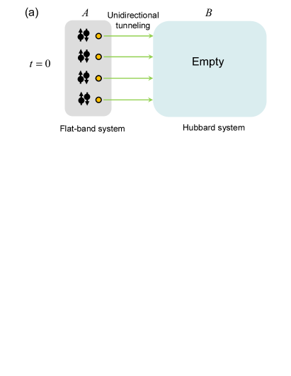
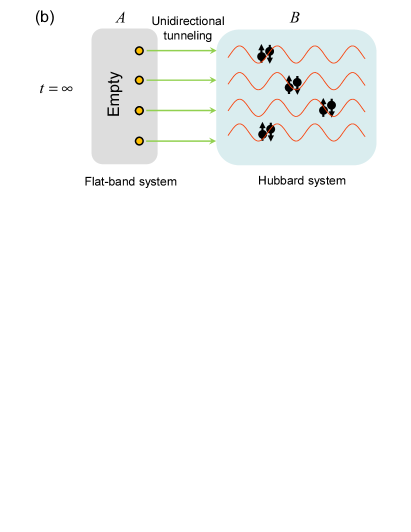
Figure 1: The system is consisted of two subsystems A and B, which is connected by unidirectional hoppings. A is a interaction-free system with trivial flat-band, while B is a Hubbard system, which supports $\eta$-pairing eigenstates. At $t=0$, A is fully filled as trivial insulating state and B is empty. When the unidirectional hoppings switch on, the probability flow from A to B. After long time, subsystem A becomes empty and subsystem B is in an $\eta$-pairing state, a condensation of bound pairs.

In general, the time dynamics of Hermitian many-body quantum systems has long been an elusive subject, due to the complexity induced by the particle-particle interactions. The main obstacle is that the evolved state is not easily predictable in most cases. Nevertheless, this difficulty may be avoided in a well-designed non-Hermitian system, since the EP in a non-Hermitian system admits a peculiar dynamics: the final state being a particular eigenstate, coalescing state Berry2004 ; Heiss2012 ; Miri2019 ; Zhang2020 ; JL . The key point is the exceptional dynamics, which allows particles pumping from the source subsystem to the central subsystem, realizing the dynamical preparation of many-body quantum states. In present work, we study the dynamic transition from a trivial insulating state to an $\eta$-pairing state in a composite non-Hermitian Hubbard system. The system is consisted of two subsystems A and B, which is connected by unidirectional hoppings. Based on the performance of the system at EP, a scheme that produces a nonequilibrium steady superconducting-like state is proposed. Specifically, for an initial state with fully filled in A, but empty in B, unidirectional hoppings can drive it to the resonant coalescing state that favors superconductivity manifested by the ODLRO. Such a dynamical scheme can be realized no matter how the shapes of the two sublattices of the composite system. Therefore, our finding is distinct from the previous investigations Kaneko ; Tindall ; ZXZPRB2 , and provides a quantum casting mechanism for generating superconductivity through nonequilibrium dynamics. On the other hand, the remarkable observation from our work can trigger further studies of both fundamental aspects and potential applications of composite non-Hermitian many-body systems.

The rest of this paper is organized as followed. In Section II, we present the model and its properties relating to $\eta$ operators, or $\eta$-symmetry. Section III is devoted to doublon effective Hamiltonian which captures the physics in a fixed energy shell. In Section IV, we present the Jordan form with high-order EP based on the effective Hamiltonian. In Section V, numerical simulations are performed to estimate the efficiency of our scheme in various values of correlation strengths. Section VI concludes this paper. Some nonessential details of our calculation are placed in Appendixes.

II Model and $\eta$ operators

We consider a composite non-Hermitian system, described by the Hamiltonian

$$H=H_{\mathrm{A}}+H_{\mathrm{B}}+H_{\mathrm{AB}},$$ (1)

with Hermitian terms

$$H_{\mathrm{A}} = \frac{U}{2}\sum_{i=1}^{N_{a}}(a_{i,\uparrow}^{{\dagger}}a_{i,\uparrow}+a_{i,\downarrow}^{{\dagger}}a_{i,\downarrow}),$$ (2)

$$H_{\mathrm{B}} = \sum_{\sigma=\uparrow,\downarrow}\sum_{i,j=1}^{N_{b}}(J_{ij}b_{i,\sigma}^{{\dagger}}b_{j,\sigma}+\mathrm{H.c.})+U\sum_{i=1}^{N_{b}}b_{i,\uparrow}^{{\dagger}}b_{i,\downarrow}^{{\dagger}}b_{i,\downarrow}b_{i,\uparrow},$$

and the non-Hermitian term

$$H_{\mathrm{AB}}=\sum_{\sigma=\uparrow,\downarrow}\sum_{i=1}^{N_{a}}\sum_{j=1}^{N_{b}}\kappa_{ij}b_{j,\sigma}^{{\dagger}}a_{i,\sigma},$$ (3)

where $a_{i,\sigma}$ and $b_{j,\sigma}$ are fermion operators with spin$-\frac{1}{2}$ polarization $\sigma=\uparrow,\downarrow$ in lattices $N_{a}$ and $N_{b}$, respectively. The parameters $J_{ij}$ ($i,j\in N_{b},i\neq j$) and $\kappa_{ij}$ ($i\in N_{a},j\in N_{b}$) are intra- and inter-cluster hopping strengths, and taken to be real in this paper. Here both $H_{\mathrm{A}}$ and $H_{\mathrm{B}}$ are Hermitian, describing the source system and the central system, respectively. $H_{\mathrm{A}}$ is an interaction-free system with trivial full flat band, while $H_{\mathrm{B}}$ is a standard Hubbard model, which is restricted to be the bipartite lattice. In particular, the key features of the setup are (i) $H_{\mathrm{AB}}$ is non-Hermitian, representing unidirectional tunnelings between two subsystems $H_{\mathrm{A}}$ and $H_{\mathrm{B}}$. (ii) The on-site potential of a pair of fermions in $H_{\mathrm{A}}$ is identical to the on-site repulsion in $H_{\mathrm{B}}$, but a little difference will not affect the scheme since the EP dynamics can be extended to the near-EP dynamics YXMPRB . The schematic of the system is presented in Fig. 1.

We define two $\eta$ operators for two subsystems

$$\eta_{\mathrm{A}}^{{\dagger}} = \sum_{i=1}^{N_{a}}\eta_{\mathrm{A},i}^{{\dagger}}=\sum_{i=1}^{N_{a}}\alpha_{i}a_{i,\uparrow}^{{\dagger}}a_{i,\downarrow}^{{\dagger}},$$ (4)

$$\eta_{\mathrm{B}}^{{\dagger}} = \sum_{i=1}^{N_{b}}\eta_{\mathrm{B},i}^{{\dagger}}=\sum_{i=1}^{N_{b}}\beta_{i}b_{i,\uparrow}^{{\dagger}}b_{i,\downarrow}^{{\dagger}},$$ (5)

where $\alpha_{i}=\pm 1$ can be taken arbitrarily, since there are no tunnelings between any two sites in the subsystem $A$, while $\beta_{i}=1$ and $-1$, for the different sublattice $i$ belongs to in the bipartite lattice $B$. It can be shown that both operators satisfy

$$\left[H_{\mathrm{A}},\eta_{\mathrm{A}}^{{\dagger}}\right]=U\eta_{\mathrm{A}}^{{\dagger}},\left[H_{\mathrm{B}},\eta_{\mathrm{B}}^{{\dagger}}\right]=U\eta_{\mathrm{B}}^{{\dagger}},$$ (6)

which can be utilized to construct the eigenstates of $H_{\mathrm{A}}$, $H_{\mathrm{B}}$, $H_{\mathrm{A}}+H_{\mathrm{B}}$,

$$\left|n\right\rangle_{\mathrm{A}} = \frac{1}{\sqrt{\Omega_{\mathrm{A},n}}}\left(\eta_{\mathrm{A}}^{{\dagger}}\right)^{n}\left|\text{Vac}\right\rangle,$$ (7)

$$\left|m\right\rangle_{\mathrm{B}} = \frac{1}{\sqrt{\Omega_{\mathrm{B},m}}}\left(\eta_{\mathrm{B}}^{{\dagger}}\right)^{m}\left|\text{Vac}\right\rangle,$$ (8)

where $\Omega_{\mathrm{A},n}=\left(n!\right)^{2}C_{N_{a}}^{n}$ and $\Omega_{\mathrm{B},m}=\left(m!\right)^{2}C_{N_{b}}^{m}$ are normalization factors.

$$H_{\mathrm{A}}\left|n\right\rangle_{\mathrm{A}}=nU\left|n\right\rangle_{\mathrm{A}},H_{\mathrm{B}}\left|m\right\rangle_{\mathrm{B}}=mU\left|m\right\rangle_{\mathrm{B}},$$ (9)

and

$$\left(H_{\mathrm{A}}+H_{\mathrm{B}}\right)\left|n\right\rangle_{\mathrm{A}}\left|m\right\rangle_{\mathrm{B}}=\left(n+m\right)U\left|n\right\rangle_{\mathrm{A}}\left|m\right\rangle_{\mathrm{B}}.$$ (10)

We can find that the set of eigenstates $\left|n\right\rangle_{\mathrm{A}}\left|m\right\rangle_{\mathrm{B}}$ are degenerate for fixed $m+n$.

In general, an $\eta$-pairing state can be regarded as the condensation of bound pair fermions as hardcore boson. However, state $\left|n\right\rangle_{\mathrm{A}}$ is trivial since it is just one of multi-fold degenerate eigenstates. In addition, fully filled state $\left|N_{a}\right\rangle_{\mathrm{A}}$ and $\left|N_{b}\right\rangle_{\mathrm{B}}$ are insulating states and can be easily prepared. The desirable states are $\left|N_{a}\right\rangle_{\mathrm{A}}\left|m\right\rangle_{\mathrm{B}}$ and $\left|0\right\rangle_{\mathrm{A}}\left|m\right\rangle_{\mathrm{B}}$ with $1<m<N_{b}$, since both two states possess ODLRO in the subsystem B.

III Doublon effective Hamiltonian

Like most interacting many-body systems, the exact solution of $H$ is rare although states $\left|n\right\rangle_{\mathrm{A}}\left|m\right\rangle_{\mathrm{B}}$ are eigenstates of $H_{\mathrm{A}}+H_{\mathrm{B}}$. In order to capture the physics of our scheme, we will consider the problem in an energy shell. In the Hermitian system, one can employ the perturbation method to get the effective Hamiltonian. However, the corresponding theory has not been well established for the non-Hermitian system, especially for the unidirectional hopping perturbation.In two Appendixes, we have illustrated how to obtain the effective Hamiltonian of a non-Hermitian system from two perspectives. The Appendix A provides an accurate effective Hamiltonian of a two-site non-Hermitian system from the time evolution operator, while the Appendix B obtains the effective Hamiltonian of an arbitrary-sized non-Hermitian system for large $U$ limit from parameters approaching the EP.

In this work, our aim is the dynamics for a special initial state, with the subsystem A being fully occupied. It motivates us to consider pure doublon states in the subsystem B, which has the same energy shell with that of the initial state. We take the parameter $\kappa_{ij}$ as a constant $\kappa\delta_{ij}$ for simplicity. For a subspace spanned by a set of basis of doublon state $\left\{{\left|\Psi_{\mathrm{D}}^{\mathrm{B}}\left(n\right)\right\rangle,{n\in[1,N_{b}]}}\right\}$, the effective Hamiltonian can be written as

$$H_{\mathrm{B}}^{\mathrm{eff}}=\sum_{i,j=1}^{N_{b}}\frac{-4J_{ij}^{2}}{U}(\boldsymbol{\eta}_{\mathrm{B},i}\cdot\boldsymbol{\eta}_{\mathrm{B},j}-\frac{1}{4})+U\sum_{i=1}^{N_{b}}\left(\frac{1}{2}+\eta_{\mathrm{B},i}^{z}\right),$$ (11)

in the case of $U\gg\left|J_{ij}\right|$. Here a doublon state is

$${\left|\Psi_{\mathrm{D}}^{\mathrm{B}}\left(n\right)\right\rangle=}b_{j_{1},\uparrow}^{{\dagger}}b_{j_{1},\downarrow}^{{\dagger}}b_{j_{2},\uparrow}^{{\dagger}}b_{j_{2},\downarrow}^{{\dagger}}...b_{j_{n},\uparrow}^{{\dagger}}b_{j_{n},\downarrow}^{{\dagger}}\left|\text{Vac}\right\rangle,$$ (12)

with $j_{n}\in[1,N_{b}]$, and the pseudo-spin operator is defined as $\boldsymbol{\eta}_{\mathrm{B},j}=(\eta_{\mathrm{B},j}^{+}/2+\eta_{\mathrm{B},j}^{-}/2,\eta_{\mathrm{B},j}^{+}/2i-\eta_{\mathrm{B},j}^{-}/2i,\eta_{\mathrm{B},j}^{z})$ with $\eta_{\mathrm{B},j}^{+}=\beta_{j}b_{j,\uparrow}^{{\dagger}}b_{j,\downarrow}^{{\dagger}}$ and $\eta_{\mathrm{B},j}^{z}=\left(n_{\mathrm{B},j,\uparrow}+n_{\mathrm{B},j,\downarrow}-1\right)/2$.  Similarly, for a subspace spanned by a set of basis of doublon $\left\{{\left|\Psi_{\mathrm{D}}^{\mathrm{A}}\left(n\right)\right\rangle,{n\in[1,N_{a}]}}\right\}$, which means ${n}$ lattice sites in subsystem A occupied by two particles with opposite spin orientation, the effective Hamiltonian can be written as

$$H_{\mathrm{A}}^{\mathrm{eff}}=U\sum_{i=1}^{N_{a}}\left(\frac{1}{2}+\eta_{\mathrm{A},i}^{z}\right),$$ (13)

and corresponding operators obey the Lie algebra, i.e., $[\eta_{\mathrm{A},i}^{+},$ $\eta_{\mathrm{A},j}^{-}]=2\eta_{\mathrm{A},j}^{z}\delta_{ij}$ and $[\eta_{\mathrm{A},i}^{z},$ $\eta_{\mathrm{A},j}^{\pm}]=\pm\eta_{\mathrm{A},j}^{\pm}\delta_{ij}$.

Now, it turns to establish the effective Hamiltonian of the non-Hermitian term $H_{\mathrm{AB}}$. Unlike the Hermitian term, there is no unquestioned perturbation theory for the non-Hermitian perturbation, especially near the EP. In this work, we present the effective Hamiltonian $H_{\mathrm{AB}}^{\mathrm{eff}}$ from two perspectives. In two Appendixes, we show that, for the given initial state with full filling A lattice and empty B lattice, the dynamics obeys the effective Hamiltonian

$$H^{\mathrm{eff}}=H_{\mathrm{A}}^{\mathrm{eff}}+H_{\mathrm{B}}^{\mathrm{eff}}+H_{\mathrm{AB}}^{\mathrm{eff}}$$ (14)

with

$$H_{\mathrm{AB}}^{\mathrm{eff}}=\frac{4\kappa^{2}}{U}\sum_{i}\eta_{\mathrm{A,}i}^{-}\eta_{\mathrm{B,}i}^{+},$$ (15)

where

$$\eta_{\mathrm{A},i}^{-}=\left(-1\right)^{i}a_{i,\downarrow}a_{i,\uparrow},\eta_{\mathrm{B},i}^{+}=\left(-1\right)^{i}b_{i,\uparrow}^{{\dagger}}b_{i,\downarrow}^{{\dagger}}.$$ (16)

It is clear that $H_{\mathrm{AB}}^{\mathrm{eff}}$ is still a non-Hermitian term which describes a unidirectional hopping of a doublon or magnon from the point of view of spin wave.

Defining a total pseudo-spin operator

$$\eta^{z}=\sum_{i=1}^{N_{a}}\eta_{\mathrm{A},i}^{z}+\sum_{j=1}^{N_{b}}\eta_{\mathrm{B},j}^{z},$$ (17)

we note that $\eta^{z}$ is conservative for the Hamiltonian $H^{\mathrm{eff}}$ due to the commutation relation

$$\left[\eta^{z},H^{\mathrm{eff}}\right]=0,$$ (18)

which ensures that the Hilbert space of $H^{\mathrm{eff}}$ can be decomposed into many invariant subspaces labeled by the eigenvalues of $\eta^{z}$, i.e., $2\eta^{z}=-N_{a}-N_{b}$, $-N_{a}-N_{b}+1$,…, $N_{a}+N_{b}-1$, $N_{a}+N_{b}$. In this work, we only focus on the subspace with $\eta^{z}=\left(N_{a}-N_{b}\right)/2$ ($N_{a}<N_{b}$), which contains the initial state with fully filling A sublattices and empty B sublattices, i.e., $\prod_{i=1}^{N_{a}}a_{i,\uparrow}^{{\dagger}}a_{i,\downarrow}^{{\dagger}}\left|\text{Vac}\right\rangle$.

IV Jordan form with high-order EP

In the above, we know that there are many degenerate eigenstates for $H_{\mathrm{A}}+H_{\mathrm{B}}$, which may become coalescing states when the proper non-Hermitian term is added WPARXIV . For non-Hermitian operators, when the EP appears, there are eigenstates coalesce into one state, leading to an incomplete Hilbert space Berry2004 ; Heiss2012 ; Miri2019 ; Zhang2020 . Mathematically, it relates to the Jordan block form in the matrix Kato ; Muller ; Moiseyev ; Emil . Remarkably, the peculiar features around the EP have sparked tremendous attention to the classical and quantum photonic systems. The corresponding intriguing dynamical phenomena include asymmetric mode switching Doppler2016 , topological energy transfer Xu2016 , robust wireless power transfer Assawaworrarit2017 , and enhanced sensitivity Wiersig2014 ; Wiersig2016 ; Hodaei2017 ; Chen2017 depending on their EP degeneracies. Many works have been devoted to the formation of the EP and corresponding topological characterization in both theoretical and experimental aspects Ding2016 ; Xiao2019 ; Pan2019 . In this work, we employ the EP dynamics to prepare states with ODLRO. We start with the Jordan form with high-order EP.

Considering two degenerate eigenstates $\left|A\right\rangle$ and $\left|B\right\rangle$ of the Hermitian Hamiltonian $H_{\mathrm{A}}+H_{\mathrm{B}}$, where

$$\left|A\right\rangle = \left|N_{a}\right\rangle_{\mathrm{A}}\left|0\right\rangle_{\mathrm{B}}=\frac{1}{\sqrt{\Omega_{\mathrm{A},N_{a}}}}\left(\eta_{\mathrm{A}}^{{\dagger}}\right)^{N_{a}}\left|\text{Vac}\right\rangle,$$ (19)

$$\left|B\right\rangle = \left|0\right\rangle_{\mathrm{A}}\left|N_{a}\right\rangle_{\mathrm{B}}=\frac{1}{\sqrt{\Omega_{\mathrm{B},N_{a}}}}\left(\eta_{\mathrm{B}}^{{\dagger}}\right)^{N_{a}}\left|\text{Vac}\right\rangle,$$ (20)

we have

$$H\left|B\right\rangle=N_{a}U\left|B\right\rangle,H^{{\dagger}}\left|A\right\rangle=N_{a}U\left|A\right\rangle,$$ (21)

due to the facts

$$H_{\mathrm{AB}}\left|0\right\rangle_{\mathrm{A}}\left|N_{a}\right\rangle_{\mathrm{B}}=0,\left(H_{\mathrm{AB}}\right)^{{\dagger}}\left|N_{a}\right\rangle_{\mathrm{A}}\left|0\right\rangle_{\mathrm{B}}=0.$$ (22)

It means that two states $\left|A\right\rangle$ and $\left|B\right\rangle$ are mutually biorthogonal conjugate and $\langle A\left|B\right\rangle$ is the biorthogonal norm of them. On the other hand, we have

$$\langle A\left|B\right\rangle=0.$$ (23)

The vanishing norm indicates that state $\left|B\right\rangle$($\left|A\right\rangle$) is the coalescing state of $H$($H^{{\dagger}}$), or Hamiltonians $H$ and $H^{{\dagger}}$ get an EP.

However, it is a little hard to determine the corresponding Jordan block form and the order of the EP. In the following, we estimate the order in large $U$ limit. At first, the above analysis for two states $\left|A\right\rangle$ and $\left|B\right\rangle$ is applicable for the effective Hamiltonian $H^{\mathrm{eff}}$. This means that there is an EP in the invariant subspace with $\eta^{z}=\left(N_{a}-N_{b}\right)/2$, and dimension $C_{N_{a}+N_{b}}^{N_{a}}$. The order of such an EP is determined by the corresponding Jordan block. Second, when we consider a complete set of degenerate eigenstates of the Hermitian Hamiltonian $H_{\mathrm{A}}+H_{\mathrm{B}}$ in this subspace, which are denoted as $\left\{\left|n\right\rangle_{\mathrm{A}}\left|m\right\rangle_{\mathrm{B}}\right\}$ ($n\in\left[0,N_{a}\right],N_{a}\leqslant N_{b}$) with fixed $m+n=N_{a}$, the effective Hamiltonian can be expressed as an $\left(N_{a}+1\right)\times\left(N_{a}+1\right)$ matrix $M$ with nonzero matrix elements

$$\left(M\right)_{N_{a}+1-n,N_{a}-n}$$ (24)

$$= \left\langle N_{a}-n\right|_{\mathrm{B}}\left\langle n\right|_{\mathrm{A}}H^{\mathrm{eff}}\left|n+1\right\rangle_{\mathrm{A}}\left|N_{a}-n-1\right\rangle_{\mathrm{B}}$$

$$= \frac{4\kappa^{2}}{U}\frac{N_{a}-n}{N_{b}}\sqrt{\left(n+1\right)\left(N_{b}-N_{a}+n+1\right)}$$

with $n=\left[0,N_{a}-1\right]$, and

$$\left(M\right)_{N_{a}+1-n,N_{a}+1-n}$$ (25)

$$= \left\langle N_{a}-n\right|_{\mathrm{B}}\left\langle n\right|_{\mathrm{A}}H^{\mathrm{eff}}\left|n\right\rangle_{\mathrm{A}}\left|N_{a}-n\right\rangle_{\mathrm{B}}$$

$$= N_{a}U$$

with $n=\left[0,N_{a}\right]$. It is obviously an $\left(N_{a}+1\right)$-order Jordan block, satisfying

$$\left[\left(M-N_{a}UI\right)^{N_{a}}\right]_{ij}=\prod\limits_{n=0}^{N_{a}-1}\frac{4\kappa^{2}}{U}\frac{N_{a}-n}{N_{b}}$$

$$\times\sqrt{\left(n+1\right)\left(N_{b}-N_{a}+n+1\right)}\delta_{N_{a}+1,1}.$$ (26)

where $I$ is the unit matrix. In other words, matrix $\left(M-N_{a}UI\right)$ is a nilpotent matrix, i.e.,

$$\left(M-N_{a}UI\right)^{N_{a}+1}=0.$$ (27)

Taking $N_{a}=N_{b}=4$, for example, the matrix has the form

$$M=\frac{2\kappa^{2}}{U}\left(\begin{array}[]{ccccc}0&0&0&0&0\\ 2&0&0&0&0\\ 0&3&0&0&0\\ 0&0&3&0&0\\ 0&0&0&2&0\end{array}\right)+4UI,$$ (28)

which possesses a single eigenvector $\left(\begin{array}[]{ccccc}0&0&0&0&1\end{array}\right)^{T}$.

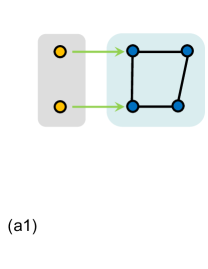
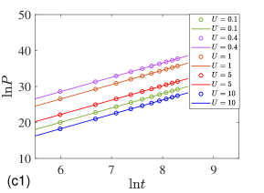
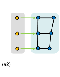
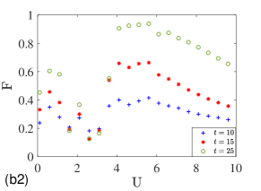
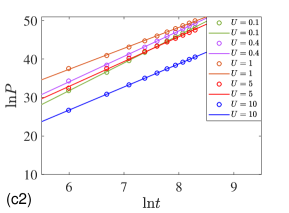
Figure 2: Schematic illustration of (a1) 6 sites composite non-Hermitian system with 4 filled particles and (a2) 9 sites composite non-Hermitian system with 6 filled particles concerned in the following numerical simulations. The parameters are $\kappa=1$, (a1)-(c1) $N_{a}=2$, $N_{b}=4$, $J_{ij}=0.75$, $1.17$, $0.68$, $1.02$; (a2)-(c2) $N_{a}=3$, $N_{b}=6$, $J_{ij}=0.75$, $1.17$, $0.68$, $1.02$, $0.87$, $0.61$, $0.72$. (b1) and (b2) are plots of fidelity $F(t)$ defined in Eq. (39). Three typical values of $t$ are taken and indicated in the panels. The numerical data oscillate at small $U$ values and the optimal $U$ occurs around $U=5$. (c1) and (c2) show the scaling law of probability $P$ defined in Eq. (38) as a function of $t$ for different value of $U$. Different colored dots represent the numerical date, which are fitted by different colored solid lines (c1) $\ln P=3.99\ln t-3.96$, $\ln P=3.97\ln t+4.77$, $\ln P=3.98\ln t+2.67$, $\ln P=3.99\ln t-1.81$, $\ln P=4.00\ln t-5.76$ and (c2) $\ln P=7.20\ln t-11.40$, $\ln P=6.61\ln t-5.56$, $\ln P=5.44\ln t+4.66$, $\ln P=6.45\ln t-5.80$, $\ln P=6.00\ln t-9.26$ from $U=0.1$ to $U=10$ respectively.

The dynamics for any states in this subspace is governed by the time evolution operator

$$U(t)=e^{-iMt}=e^{-iN_{a}Ut}\sum_{l=0}^{N_{a}}\frac{1}{l!}\left[-i\left(M-N_{a}UI\right)t\right]^{l}.$$ (29)

It indicates that for the initial state $\left|\Psi(0)\right\rangle=\left|A\right\rangle$, we have

$$\left|\Psi(t)\right\rangle = e^{-iMt}\left|A\right\rangle$$ (30)

$$= e^{-iN_{a}Ut}\left(\begin{array}[]{cccccc}1&f_{1}&...&f_{q}&...&f_{N_{a}}\end{array}\right)^{T},$$ (32)

where the elements

$$f_{q} = \sqrt{A_{N_{a}}^{q}A_{N_{b}}^{q}}\left(\frac{-4i\kappa^{2}t}{UN_{b}}\right)^{q},q\in[1,N_{a}]$$ (33)

$$A_{N_{a}}^{q} = \frac{N_{a}!}{\left(N_{a}-q\right)!},A_{N_{b}}^{q}=\frac{N_{b}!}{\left(N_{b}-q\right)!},$$ (34)

and

$$\left|\left|\Psi\left(t\right)\right\rangle\right|=\sqrt{1+\sum\limits_{q=1}^{N_{a}}\left|f_{q}\right|^{2}}\approx\left|f_{N_{a}}\right|\text{ }$$ (35)

at large $t\gg\frac{UN_{b}}{\kappa^{2}}$. Setting the target state as

$$\left|\Psi_{\text{target}}\right\rangle=\left|B\right\rangle,$$ (36)

we have the fidelity

$$F(t)=\frac{\left|\left\langle\Psi_{\text{target}}\right|\Psi\left(t\right)\rangle\right|}{\left|\left|\Psi\left(t\right)\right\rangle\right|}=\frac{\left|f_{N_{a}}\right|}{\left|\left|\Psi\left(t\right)\right\rangle\right|}\approx 1,$$ (37)

which indicates that state $\left|\Psi_{\text{target}}\right\rangle$ becomes dominant in the evolved state $\left|\Psi\left(t\right)\right\rangle$ at large $t\gg\frac{UN_{b}}{\kappa^{2}}$. The increasing behavior of $\left|\left|\Psi\left(t\right)\right\rangle\right|$ obeying $\left|\left|\Psi\left(t\right)\right\rangle\right|^{2}\propto t^{2N_{a}}$ within large $t$ region is also a dynamic demonstration for the order of the Jordan block. This analytical analysis shows that the speed of relaxation of ODLRO pair state depends on the order of the EP, which is determined by the number of pairs. Furthermore, we would like to address two points. (i) The non-Hermitian effective Hamiltonian $H_{\mathrm{AB}}^{\mathrm{eff}}$ is obtained from the simplest case with $N_{a}=N_{b}=1$ in the Appendix A. Its validity for large systems is illustrated in the Appendix B for large $U$ limit and from the perspective of parameters approaching the EP. (ii) The power behavior of $\left|\left|\Psi\left(t\right)\right\rangle\right|$ requires large $t$. However, in practice, $F(t)$ may approach unit before this time domain.

V Dynamic transition

The above analysis provides a prediction about the dynamic transition from an insulating state to an $\eta$-pairing state in a composite non-Hermitian system. The composite system is consisted of two parts (or two layers), one is a trivial system (source system) constructed by a set of isolated sites, while the other is a Hubbard model (central system), which supports $\eta$-pairing eigenstates. Initially, two subsystems are separated and the source system is fully filled by electrons, being in an insulating state, while the central system is empty. The decoupling between two subsystems can be achieved in two ways, i.e., the pre-quench Hamiltonian can be setted by (a) taking the chemical potential on source system far from the resonant energy of the central system; (b) switching off the tunneling terms between two subsystems directly under the resonant condition. The post-quench Hamiltonian is then $H_{\mathrm{A}}+H_{\mathrm{B}}+H_{\mathrm{AB}}$. According to our analysis, both two quench dynamics should result in steady superconducting state, realizing the dynamic transition from an insulating state to an $\eta$-pairing state.

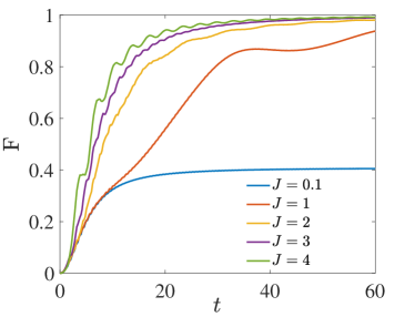
Figure 3: The Plot of $F(t)$, which is obtained by exact diagonalization of the original Hamiltonian for the finite system. The parameters are $N_{a}=2$, $N_{b}=4$, $\kappa=1$, $U=20$, $J_{ij}=J$. Several typical values of $J$ are taken and indicated in the panels.

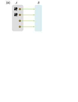
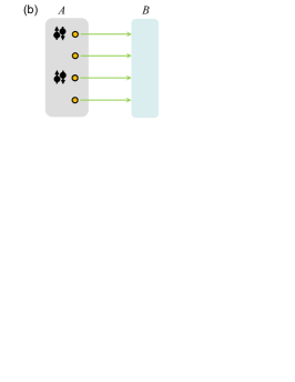
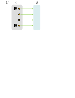
Figure 4: Schematics of the composite non-Hermitian system with different initial states. (a), (b), and (c) present three typical configurations, in which two doublons are located in different sites of system A. The analytical analysis based on the perturbation method in large $U$ limit indicates that the final states after long time are the same. Numerical simulations for finite $U$ and small-size system support this conclusion.

We perform numerical simulations on finite system with the following considerations. (i) The analysis based on the effective Hamiltonian in last section only predicts the results for large ${U}$ within large time domain. The efficiency of the scheme should be estimated from numerical simulations of the original Hamiltonian. (ii) The existence of $\eta$-pairing eigenstates are independent of the distribution of the hoppings for B sublattices. The evolved states $\left|\Psi\left(t\right)\right\rangle$ for initial states $\left|2\right\rangle_{\mathrm{A}}\left|0\right\rangle_{\mathrm{B}}$ and $\left|3\right\rangle_{\mathrm{A}}\left|0\right\rangle_{\mathrm{B}}$ in two finite systems are computed by exact diagonalization. We focus on the Dirac probability

$$P(t)=\left|\left|\Psi\left(t\right)\right\rangle\right|^{2},$$ (38)

and the fidelity

$$F(t)=\frac{1}{\sqrt{P}}\left|\left\langle\Psi_{\text{target}}\right|\Psi\left(t\right)\rangle\right|,$$ (39)

with the target states being $\left|0\right\rangle_{\mathrm{A}}\left|2\right\rangle_{\mathrm{B}}$ and $\left|0\right\rangle_{\mathrm{A}}\left|3\right\rangle_{\mathrm{B}}$, respectively. The lattice geometry and numerical results are plotted in Fig. 2. We plot the fidelity as function of ${U}$ for three typical instants. We find that there exits an optimal ${U\approx 5}$, at which the fidelity gets the maximal value. We also plot the probability ln${P(t)}$ as function of ln${t}$ to demonstrate the EP dynamic behavior. From the results of linear fitting, it can be seen that the slope of the line deviates from the predicted value for the cases with small $U$, especially for larger system. This indicates that the speed of relaxation of pair state depends on the order of the EP and the fidelity of the scheme is immune to the irregularity of the lattice. We estimated the relation of the hopping strength and the efficiency of the scheme from numerical simulations of the original Hamiltonian in Fig. 3. Within a certain range of parameters, the increase of the hopping strength will improve the efficiency of the scheme.

VI Summary and discussion

In summary, we have extended the scheme of quantum casting to interacting many-body systems. Unlike the previous work Ref. YXMPRB on non-interacting systems, the present scheme does not require the scan on the chemical potential of the source system. Our findings offer a method for the efficient preparation of correlated states and are expected to be necessary and insightful for quantum engineering. The key point is the exceptional dynamics, which allows particles pumping from the source subsystem to the central subsystem, realizing the dynamical preparation of many-body quantum states. It is due to the resonance between the initial state and the target state. Accordingly, there is a class of initial states (see Fig. 4) evolving to the same final state after long time. Numerical simulations for finite $U$ and small-size system support this conclusion. In this sense, such a scheme can be applied to other interacting many-body systems. On the other hand, considering a quench process with the pre-quench Hamiltonian being $H_{\mathrm{A}}+H_{\mathrm{B}}$, and the post-quench Hamiltonian being $H_{\mathrm{A}}+H_{\mathrm{B}}+H_{\mathrm{AB}}$, the Loschmidt echo $\left|L\right|^{2}=\left|\left\langle\Psi\left(0\right)\right|\Psi\left(t\right)\rangle\right|^{2}$ should turn to zero after a long time for a finite system. It may predict an asymptotic dynamic quantum phase transition (DQPT) QD3 in thermodynamic limit, i.e., $\left|L\right|^{2}$ decays rapidly, rather than vanishes at a finite instant in a standard DQPT. The final answer depends on the scaling behavior of $\left|L\right|^{2}$, that is an open question at the present stage.

Appendix A

In this Appendix, we present a derivation of the effective Hamiltonian in the doublon subspace for the tunneling term between two subsystems A and B. We will obtain the effective Hamiltonian from the time evolution operator rather than the perturbation method due to the concern with the availability of it for a non-Hermitian system at exceptional point.

Consider a two-site Hamiltonian

$$H_{\mathrm{conn}}=\sum_{\sigma=\uparrow,\downarrow}\kappa b_{\sigma}^{{\dagger}}a_{\sigma}+Ub_{\uparrow}^{{\dagger}}b_{\downarrow}^{{\dagger}}b_{\downarrow}b_{\uparrow}+\frac{U}{2}(a_{\uparrow}^{{\dagger}}a_{\uparrow}+a_{\downarrow}^{{\dagger}}a_{\downarrow}),$$ (40)

which describes the connection between any two sites among A and B subsystems. We neglect the subscripts of the operators for the sake of simplicity. We start from the matrix representation of the Hamiltonian in the invariant subspace spanned by the basis set

$$\left|1\right\rangle = \left|\uparrow\downarrow\right\rangle_{\mathrm{A}}\left|0\right\rangle_{\mathrm{B}}=a_{\uparrow}^{{\dagger}}a_{\downarrow}^{{\dagger}}\left|\mathrm{Vac}\right\rangle$$ (41)

$$\left|2\right\rangle = \left|0\right\rangle_{\mathrm{A}}\left|\uparrow\downarrow\right\rangle_{\mathrm{B}}=b_{\uparrow}^{{\dagger}}b_{\downarrow}^{{\dagger}}\left|\mathrm{Vac}\right\rangle$$

$$\left|3\right\rangle = \left|\uparrow\right\rangle_{\mathrm{A}}\left|\downarrow\right\rangle_{\mathrm{B}}=a_{\uparrow}^{{\dagger}}b_{\downarrow}^{{\dagger}}\left|\mathrm{Vac}\right\rangle$$

$$\left|4\right\rangle = \left|\downarrow\right\rangle_{\mathrm{A}}\left|\uparrow\right\rangle_{\mathrm{B}}=a_{\downarrow}^{{\dagger}}b_{\uparrow}^{{\dagger}}\left|\mathrm{Vac}\right\rangle$$

is

$$h=\left(\begin{array}[]{cccc}U&0&0&0\\ 0&U&\kappa&-\kappa\\ \kappa&0&\frac{U}{2}&0\\ -\kappa&0&0&\frac{U}{2}\end{array}\right),$$ (42)

which contains a $2\times 2$ Jordan block for nonzero $U$. The solution of matrix consists $3$ eigenvectors $\left|\phi_{c}\right\rangle$, $\left|\phi_{3}\right\rangle$ and $\left|\phi_{4}\right\rangle$, with eigenvalues $U$, $U/2$, and $U/2$, respectively. The explicit form of the vectors is

$$\left|\phi_{a}\right\rangle = \left(\begin{array}[]{c}1\\ 0\\ \frac{2\kappa}{U}\\ -\frac{2\kappa}{U}\end{array}\right),\left|\phi_{c}\right\rangle=\left(\begin{array}[]{c}0\\ 1\\ 0\\ 0\end{array}\right),$$ (51)

$$\left|\phi_{3}\right\rangle = \left(\begin{array}[]{c}0\\ -\frac{2\kappa}{U}\\ 1\\ 0\end{array}\right),\left|\phi_{4}\right\rangle=\left(\begin{array}[]{c}0\\ \frac{2\kappa}{U}\\ 0\\ 1\end{array}\right),$$ (60)

where $\left|\phi_{c}\right\rangle$ is the coalescing vector and $\left|\phi_{a}\right\rangle$ is the corresponding auxiliary vector, satisfying

$$\left(h-UI\right)\left|\phi_{a}\right\rangle=\left|\phi_{c}\right\rangle,$$ (61)

where $I$ is the unit matrix. We would like to point out that in the case of $U=0$, $h$ contains a $3\times 3$ Jordan block. The solution of matrix consists $2$ eigenvectors $\left|\phi_{c}\right\rangle$ and $\left|\phi_{4}\right\rangle$, with the same eigenvalue $0$. The explicit form of the vectors is

$$\left|\phi_{a}\right\rangle=\left(\begin{array}[]{c}1\\ 0\\ 0\\ 0\end{array}\right),\left|\phi_{c}\right\rangle=\left(\begin{array}[]{c}0\\ 1\\ 0\\ 0\end{array}\right),\left|\phi_{4}\right\rangle=\left(\begin{array}[]{c}0\\ 0\\ 1\\ 1\end{array}\right),$$ (62)

where $\left|\phi_{c}\right\rangle$ is the coalescing vector and $\left|\phi_{a}\right\rangle$ is the corresponding auxiliary vector. In this work, we only focus on the case with nonzero $U$. However, one should consider the effect of $3$-order EP when $U$ is very small. Then the time evolution operator in such a invariant subspace can be obtained as

$$e^{-iht}=e^{-itU}\left(\begin{array}[]{cccc}1&0&0&0\\ -\frac{4it\kappa^{2}}{U}-\frac{8\kappa^{2}}{U^{2}}\Lambda&1&\frac{2\kappa}{U}\Lambda&-\frac{2\kappa}{U}\Lambda\\ \frac{2\kappa}{U}\Lambda&0&e^{\frac{itU}{2}}&0\\ -\frac{2\kappa}{U}\Lambda&0&0&e^{\frac{itU}{2}}\end{array}\right),$$ (63)

where $\Lambda=1-e^{\frac{itU}{2}}$. The time evolution of the trivial initial state $\left|\phi_{a}\right\rangle$ can be expressed as

$$\left|\Psi\left(t\right)\right\rangle=e^{-iht}\left|\phi_{a}\right\rangle=e^{-itU}\left(\begin{array}[]{c}1\\ -\frac{4it\kappa^{2}}{U}-\frac{8\kappa^{2}}{U^{2}}\Lambda\\ \frac{2\kappa}{U}\\ -\frac{2\kappa}{U}\end{array}\right).$$ (64)

We find that

$$\langle 2\left|\Psi\left(t\right)\right\rangle=-e^{-itU}\frac{4\kappa^{2}}{U}\left[it+\frac{2}{U}\left(1-e^{\frac{itU}{2}}\right)\right],$$ (65)

which can be valued within finite time scale as

$$\langle 2\left|\Psi\left(t\right)\right\rangle\approx-e^{-itU}\frac{4\kappa^{2}}{U}\left\{\begin{array}[]{cc}it,&\text{large }U\\ \frac{U}{4}t^{2},&\text{small }U\end{array}\right..$$ (66)

Note that the switching of powers of the variable $t$ is due to the cancellation of the linear $t$ term in the small $U$ limit. It accords with the above analysis about the order of Jordan block. In large $U$ limit, $U\gg\kappa$, $e^{-iht}$ reduces to a diagonal-block form

$$e^{-iht}\approx e^{-itU}\left(\begin{array}[]{cccc}1&0&0&0\\ -\frac{4it\kappa^{2}}{U}&1&0&0\\ 0&0&e^{\frac{itU}{2}}&0\\ 0&0&0&e^{\frac{itU}{2}}\end{array}\right).$$ (67)

Then in the doublon subspace spanned by $a_{\uparrow}^{{\dagger}}a_{\downarrow}^{{\dagger}}\left|\mathrm{Vac}\right\rangle$ and $b_{\uparrow}^{{\dagger}}b_{\downarrow}^{{\dagger}}\left|\mathrm{Vac}\right\rangle$, the effective Hamiltonian is

$$H_{\mathrm{conn}}^{\text{eff}}=\frac{4\kappa^{2}}{U}b_{\uparrow}^{{\dagger}}b_{\downarrow}^{{\dagger}}a_{\downarrow}a_{\uparrow}+UI_{2}.$$ (68)

Appendix B

In this appendix, we obtain the effective Hamiltonian of the the tunneling term $H_{AB}$ with arbitrary size for large $U$ limit from the perspective of parameters approaching the EP. At first, we add an unidirectional tunneling term $\lambda a_{l,\sigma}^{{\dagger}}b_{l,\sigma}$ and take the parameter $\kappa_{ij}$ as a constant $\kappa\delta_{ij}$ for simplicity. The new tunneling between two subsystems $H_{A}$ and $H_{B}$ reads

$$H_{\mathrm{AB}}^{\prime}=\sum_{\sigma=\uparrow,\downarrow}\sum_{l}\left(\kappa b_{l,\sigma}^{{\dagger}}a_{l,\sigma}+\lambda a_{l,\sigma}^{{\dagger}}b_{l,\sigma}\right).$$ (69)

We introduce a set of canonical operators

$$\bar{c}_{l,\sigma} = \sqrt{\frac{\lambda}{\kappa}}a_{l,\sigma}^{{\dagger}},c_{l,\sigma}=\sqrt{\frac{\kappa}{\lambda}}a_{l,\sigma},$$

$$\bar{d}_{l,\sigma} = b_{l,\sigma}^{{\dagger}},d_{l,\sigma}=b_{l,\sigma},$$ (70)

which obey the commutative relations

$$\left\{c_{l,\sigma},\bar{c}_{l^{\prime},\sigma^{\prime}}\right\} = \delta_{ll^{\prime}}\delta_{\sigma\sigma^{\prime}},\left\{\bar{c}_{l,\sigma},\bar{c}_{l^{\prime},\sigma^{\prime}}\right\}=\left\{c_{l,\sigma},c_{l^{\prime},\sigma^{\prime}}\right\}=0,$$

$$\left\{d_{l,\sigma},\bar{d}_{l^{\prime},\sigma^{\prime}}\right\} = \delta_{ll^{\prime}}\delta_{\sigma\sigma^{\prime}},\left\{\bar{d}_{l,\sigma},\bar{d}_{l^{\prime},\sigma^{\prime}}\right\}=\left\{d_{l,\sigma},d_{l^{\prime},\sigma^{\prime}}\right\}=0.$$

The transformation in Eq. (70) is essentially a similarity transformation with singularities at $\lambda=0$ and $\kappa=0$, beyond which it allows us to rewrite the Hamiltonian in the form

$$H_{\mathrm{AB}}^{\prime}=\sum_{\sigma=\uparrow,\downarrow}\sum_{l}\left[\sqrt{\lambda\kappa}\bar{d}_{l,\sigma}c_{l,\sigma}+\sqrt{\lambda\kappa}\bar{c}_{l,\sigma}d_{l,\sigma}\right].$$ (72)

So far, $H_{\mathrm{AB}}^{\prime}$ has become a Hermitian Hamiltonian, which allows us to employ the perturbation method to get the effective Hamiltonian

$$\left(H_{\mathrm{AB}}^{\prime}\right)^{\mathrm{eff}} = -\frac{8}{U}\sum_{l}(-\frac{\kappa^{2}\eta_{\mathrm{A},l}^{-}\eta_{\mathrm{B},l}^{+}}{2}$$

$$-\frac{\lambda^{2}\eta_{\mathrm{A},l}^{+}\eta_{\mathrm{B},l}^{-}}{2}+\lambda\kappa\eta_{\mathrm{A},l}^{z}\eta_{\mathrm{B},l}^{z}-\frac{\lambda\kappa}{4}).$$

Although the above solution is only true for nonzero $\lambda$, one can extrapolate the approximate solution at $\lambda=0$ by taking $\lambda\rightarrow 0$. In the limit of zero $\lambda$, we have $H_{\mathrm{AB}}^{\prime}\rightarrow H_{\mathrm{AB}}$ and $\left(H_{\mathrm{AB}}^{\prime}\right)^{\mathrm{eff}}\rightarrow H_{\mathrm{AB}}^{\mathrm{eff}}.$

References

- (1) J. Hubbard, Electron correlations in narrow energy bands, Proc. R. Soc. A 276, 238 (1963).
- (2) S. Jochim, M. Bartenstein, A. Altmeyer, G. Hendl, S. Riedl, C. Chin, J. Hecker Denschlag, and R. Grimm, Bose-Einstein Condensation of Molecules, Science 302, 2101 (2003).
- (3) M. Greiner, C. A. Regal, and D. S. Jin, Emergence of a molecular Bose–Einstein condensate from a Fermi gas, Nature (London) 426, 537 (2003).
- (4) M. P. A. Fisher, P. B. Weichman, G. Grinstein, and D. S. Fisher, Boson localization and the superfluid-insulator transition, Phys. Rev. B 40, 546 (1989).
- (5) A. Georges, G. Kotliar, W. Krauth, and M. J. Rozenberg, Dynamical mean-field theory of strongly correlated fermion systems and the limit of infinite dimensions, Rev. Mod. Phys. 68, 13 (1996).
- (6) B. Keimer, S. A. Kivelson, M. R. Norman, S. Uchida, and J. Zaanen, From quantum matter to high-temperature superconductivity in copper oxides, Nature (London) 518, 179 (2015).
- (7) P. A. Lee, N. Nagaosa, and X.-G. Wen, Doping a mott insulator: Physics of high-temperature superconductivity, Rev. Mod. Phys. 78, 17 (2006).
- (8) C. N. Yang, pairing and off-diagonal long-range order in a hubbard model, Phys. Rev. Lett. 63, 2144 (1989).
- (9) S. Choi, J. Choi, R. Landig, G. Kucsko, H. Zhou, J. Isoya, F. Jelezko, S. Onoda, H. Sumiya, V. Khemani, C. v. Keyserlingk, N. Y. Yao, E. Demler, and M. D. Lukin, Observation of discrete time-crystalline order in a disordered dipolar many-body system, Nature 543, 221 (2017).
- (10) D. V. Else, B. Bauer, and C. Nayak, Floquet time crystals, Phys. Rev. Lett. 117, 090402 (2016).
- (11) V. Khemani, A. Lazarides, R. Moessner, and S. L. Sondhi, Phase structure of driven quantum systems, Phys. Rev. Lett. 116, 250401 (2016).
- (12) N. H. Lindner, G. Refael, and V. Galitski, Floquet Topological Insulator in Semiconductor Quantum Wells, Nat. Phys. 7, 490 (2011).
- (13) T. Kaneko, T. Shirakawa, S. Sorella, and S. Yunoki, Photoinduced Pairing in the Hubbard Model, Phys. Rev. Lett. 122, 077002 (2019).
- (14) J. Tindall, B. Buča, J. R. Coulthard, and D. Jaksch, Heating-Induced Long-Range Pairing in the Hubbard Model, Phys. Rev. Lett. 123, 030603 (2019).
- (15) X. Z. Zhang and Z. Song, -pairing ground states in the non-Hermitian Hubbard model, Phys. Rev. B 103, 235153 (2021).
- (16) X. M. Yang and Z. Song, Resonant generation of a p-wave Cooper pair in a non-Hermitian Kitaev chain at the exceptional point, Phys. Rev. A 102, 022219 (2020).
- (17) M. Rigol, V. Dunjko, and M. Olshanii, Thermalization and Its Mechanism for Generic Isolated Quantum Systems, Nature (London) 452, 854 (2008).
- (18) J. Eisert, M. Friesdorf, and C. Gogolin, Quantum Many-Body Systems out of Equilibrium, Nat. Phys. 11, 124 (2015).
- (19) M. Heyl, Dynamical quantum phase transitions: A brief survey, Europhys. Lett. 125, 26001 (2019).
- (20) X. M. Yang and Z. Song, Quantum mold casting for topological insulating and edge states, Phys. Rev. B 103, 094307 (2021).
- (21) M. V. Berry, Physics of nonhermitian degeneracies, Czech. J. Phys. 54, 1039 (2004).
- (22) W. D. Heiss, The physics of exceptional points, J. Phys. A: Math. Theor. 45, 444016 (2012).
- (23) M.-A. Miri and A. Alú, Exceptional points in optics and photonics, Science 363, eaar7709 (2019).
- (24) X. Zhang and J. Gong, Non-Hermitian Floquet topological phases: Exceptional points, coalescent edge modes, and the skin effect, Phys. Rev. B 101, 045415 (2020).
- (25) L. Jin, P. Wang, and Z. Song, Su-Schrieffer-Heeger chain with one pair of -symmetric defects, Sci. Rep. 7, 5903 (2017).
- (26) P. Wang, K. L. Zhang, and Z. Song, Transition from degeneracy to coalescence: theorem and applications, Phys. Rev. B 104, 245406 (2021).
- (27) T. Kato, Perturbation theory of linear operator (Springer, Berlin, 1966).
- (28) M. Muller and I. Rotter, Exceptional points in open quantum systems, J. Phys. A: Math. Theor. 41, 244018 (2008).
- (29) N. Moiseyev, Non-Hermitian Quantum Mechanics (Cambridge University Press, Cambridge, UK, 2011).
- (30) Emil J. Bergholtz, Jan Carl Budich, and Flore K. Kunst, Exceptional topology of non-Hermitian systems, Rev. Mod. Phys. 93, 015005 (2021).
- (31) J. Doppler, A. A. Mailybaev, J. Böhm, U. Kuhl, A. Girschik, F. Libisch, T. J. Milburn, P. Rabl, N. Moiseyev, and S. Rotter, Dynamically encircling an exceptional point for asymmetric mode switching, Nature 537, 76 (2016).
- (32) H. Xu, D. Mason, L. Jiang, and J. G. E. Harris, Topological energy transfer in an optomechanical system with exceptional points, Nature 537, 80 (2016).
- (33) S. Assawaworrarit, X. Yu, and S. Fan, Robust wireless power transfer using a nonlinear parity–time-symmetric circuit, Nature 546, 387 (2017).
- (34) J. Wiersig, Enhancing the sensitivity of frequency and energy splitting detection by using exceptional points: application to microcavity sensors for single-particle detection, Phys. Rev. Lett. 112, 203901 (2014).
- (35) J. Wiersig, Sensors operating at exceptional points: general theory, Phys. Rev. A 93, 033809 (2016).
- (36) H. Hodaei, A. U. Hassan, S. Wittek, H. Garcia-Gracia, R. El-Ganainy, D. N. Christodoulides, and M. Khajavikhan, Enhanced sensitivity at higher-order exceptional points, Nature 548, 187 (2017).
- (37) W. Chen, Ş. Kaya Özdemir, G. Zhao, J. Wiersig, and L. Yang, Exceptional points enhance sensing in an optical microcavity, Nature 548, 192 (2017).
- (38) K. Ding, G. Ma, M. Xiao, Z. Q. Zhang, and C. T. Chan, Emergence, coalescence, and topological properties of multiple exceptional points and their experimental realization, Phys. Rev. X 6, 021007 (2016).
- (39) Y.-X. Xiao, Z.-Q. Zhang, Z. H. Hang, and C. T. Chan, Anisotropic exceptional points of arbitrary order, Phys. Rev. B 99, 241403(R) (2019).
- (40) L. Pan, S. Chen, and X. Cui, Interacting non-Hermitian ultracold atoms in a harmonic trap: Two-body exact solution and a high-order exceptional point, Phys. Rev. A 99, 063616 (2019).