Adaptive Density-Matrix Renormalization-Group study of the disordered antiferromagnetic spin-1/2 Heisenberg chain

Abstract

Using an adaptive strategy which enables the study of quenched disordered system via the density-matrix renormalization-group method, we compute the various ground-state spin-spin correlation measures of the spin-$1/2$ antiferromagnetic Heisenberg chain with random coupling constants, namely, the mean values of the bulk and of the end-to-end correlations, the typical value of the bulk correlations, and the distribution of the bulk correlations. Our results are in agreement with the predictions of the strong-disorder renormalization-group method. We do not find any hint of logarithmic corrections either in the bulk average correlations, which were recently reported by Shu et al. [Phys. Rev. B. 94, 174442, (2016)], or in the end-to-end average correlations. We report the existence of a logarithmic correction on the end-to-end correlations of the clean chain. Finally, we have determined that the distribution of the bulk correlations, when properly rescaled by an associated Lyapunov exponent, is a narrow and universal (disorder-independent) probability function.

Published in Phys. Rev. B 105, 104205 (2022); DOI: 10.1103/PhysRevB.105.104205

I Introduction

One-dimensional random quantum systems display a rich plethora of phenomena and are important theoretical laboratories for strongly correlated quantum phenomena. A prominent phenomenon is the infinite-randomness criticality (IRC) (Fisher, 1992). Initially, it was thought to be exclusive to one-dimensional systems. In recent decades, however, it was found in many different and seemingly unrelated model systems. To name a few, IRC governs the paramagnet–ferromagnet transition of the random transverse-field Ising model (in any dimension) (Motrunich et al., 2000; Pich et al., 1998; Kovács and Iglói, 2011; Vojta and Hoyos, 2014) and of the quenched disordered Hertz-Millis antiferromagnet (Hoyos et al., 2007a; Vojta et al., 2009) and the metal–superconductor transition of rough thin films and nanowires (Del Maestro et al., 2008, 2010). IRC is also found in out-of-equilibrium situations such as Floquet systems (Berdanier et al., 2018) and reaction-diffusion classical systems (Hooyberghs et al., 2003) (for a review, see, e.g., Refs. Iglói and Monthus, 2005; Vojta, 2006, 2010; Iglói and Monthus, 2018). Despite this plethora of theoretical situations, experimental checks of IRC are still rare. Early hints come from quasi-one-dimensional tetracyanoquinodimethan (TCNQ) compounds (Bulaevskii et al., 1972; Shchegolev, 1972; Azevedo and Clark, 1977; Tippie and Clark, 1981) [modeled by the Hamiltonian in Eq. (1)], which initiated this field of research. However, more accurate experiments and clearer signatures are still desirable. In this context, precise knowledge of the ground-state spin-spin correlation function (the main quantity studied in this work) has great relevance as it dictates the behavior of the structure factor at low temperatures (Damle et al., 2000; Hoyos et al., 2007b), which is experimentally accessible via neutron-scattering experiments. Finally, it is worth noting that, more recently, strong experimental evidence of infinite-randomness criticality was reported in itinerant magnets (Guo et al., 2008; Westerkamp et al., 2009; Ubaid-Kassis et al., 2010) (for a review, see Ref. Vojta, 2010) and in thin superconducting films (Xing et al., 2015).

A paradigmatic model exhibiting IRC is the random antiferromagnetic (AF) spin-$1/2$ XXZ chain

$$H=\sum_{i}J_{i}\left(S_{i}^{x}S_{i+1}^{x}+S_{i}^{y}S_{i+1}^{y}+\Delta S_{i}^{z}S_{i+1}^{z}\right),$$ (1)

where $\mathbf{S}_{i}$ are the usual spin-1/2 operators associated with site $i$, the antiferromagnetic coupling constants $J_{i}>0$ are independent and identically distributed random variables drawn from a distribution $P_{D}(J)$ [with $D$ parametrizing the disorder strength; see, for definiteness, Eq. (6)], and $\Delta$ is the anisotropy parameter. It is now well accepted that, for $-\frac{1}{2}<\Delta\leq 1$, the chain is critical and governed by an infinite-randomness fixed point where the arithmetic and geometric means (henceforth referred to as mean and typical values, respectively) of the spin-spin correlation function [$C_{i}^{\alpha}(r)=\left\langle S_{i}^{\alpha}S_{i+r}^{\alpha}\right\rangle$, with $\left\langle\cdots\right\rangle$ denoting the ground-state average] behave quite differently.

In the thermodynamic limit and for spins sufficiently far from each other, the mean value is

$$\overline{C_{i}^{\alpha}}(r)=\frac{\left(-1\right)^{r}}{12r^{\eta}}\begin{cases}c_{\alpha,\text{o}},&\mbox{if }r\mbox{ is odd},\\ c_{\alpha,\text{e}},&\mbox{otherwise},\end{cases}$$ (2)

with $\overline{\cdots}$ denoting the arithmetic average over the disorder configurations. The exponent $\eta=2$ is universal [i.e., does not depend on the details of $P_{D}(J)$], isotropic (i.e., $\alpha$ independent), and $\Delta$ independent (Fisher, 1994) due to an enhancement in the ground-state symmetry from SO($N$)$\rightarrow$SU($N$) (here, $N=2$), a generic feature of SO($N$)-symmetric AF random spin chains (Quito et al., 2020, 2019). The numerical prefactors $c_{\alpha,\text{o,e}}$, on the other hand, are nonuniversal (i.e., disorder dependent), anisotropic (i.e., $\alpha$ dependent), and $\Delta$ dependent. Surprisingly, it was conjectured that $c_{\alpha,\text{o}}-c_{\alpha,\text{e}}=1$ is universal if $\alpha$ is a symmetry axis, i.e., for $\alpha=z$, and for any $\alpha$ when $\Delta=1$ (Hoyos et al., 2007b).

The typical value of the spin-spin correlation function,

$$C_{\text{typ}}^{\alpha}\left(r\right)\equiv\exp\overline{\ln\left|\left\langle S_{i}^{\alpha}S_{i+r}^{\alpha}\right\rangle\right|}\approx c_{\alpha,D}\exp\left[-A_{\alpha}\times\left(r\gamma_{D}\right)^{\psi}\right],$$ (3)

behaves quite differently. It decays stretched exponentially with universal and isotropic tunneling exponent $\psi=\frac{1}{2}$ (Fisher, 1994). The numerical prefactor $A_{\alpha}$ is universal and anisotropic, and the Lyapunov exponent $\gamma_{D}$ is nonuniversal, isotropic, and $\Delta$ dependent. For the free-fermionic case $\left(\Delta=0\right)$, a single-parameter theory (Mard et al., 2014; Getelina and Hoyos, 2020) predicts that $\gamma_{D}=8\pi^{-1}\text{var}\left(\ln J\right)$ [where $\text{var}\left(x\right)=\overline{x^{2}}-\overline{x}^{2}$ is the variance]. For the generic case $\left(-\frac{1}{2}<\Delta\leq 1\right)$, however, $\gamma_{D}\propto\left[\text{var}\left(\ln J\right)\right]^{\frac{1}{3-2K}}$ with $2K=\left[1-\pi^{-1}\arccos\left(\Delta\right)\right]^{-1}$.

Results (2) and (3) stem from the fact that the ground state is a random singlet which is captured by the strong-disorder renormalization-group (SDRG) method and, supposedly, are asymptotic exact (Fisher, 1994). It is worth mentioning that, at the free-fermion point $\Delta=0$ (Henelius and Girvin, 1998; Laflorencie and Rieger, 2003; Hoyos et al., 2007b; Getelina and Hoyos, 2020) and at the isotropic Heisenberg point $\Delta=1$ (Laflorencie et al., 2004; Tran and Bonesteel, 2011; Goldsborough and Römer, 2014; Goldsborough and Evenbly, 2017), these results (among other SDRG predictions) have been confirmed with increasing numerical precision over the years (see Refs. Iglói and Monthus, 2005, 2018 and references therein). Interestingly, however, a recent ground-state quantum Monte Carlo study found a logarithmic factor in the mean correlation function (Shu et al., 2016) at the isotropic point $\Delta=1$. Namely, result (2) is corrected to

$$\overline{C^{\alpha}}(r)\sim\ln^{\sigma_{s}}r/r^{2},$$ (4)

with $0.3\apprle\sigma_{s}\apprle 0.7$. It is certainly desirable to understand the origin of this logarithmic correction, which is not predicted by the SDRG method. For the homogeneous (clean) system at the Heisenberg point $\Delta=1$ (Affleck et al., 1989; Giamarchi and Schulz, 1989; Singh et al., 1989; Hallberg et al., 1995; Affleck, 1998; Lukyanov, 1998; Hikihara and Furusaki, 1998; Sandvik, 2010) and for the dirty system at $\Delta=-\frac{1}{2}$ (where disorder is perturbatively irrelevant) (Ristivojevic et al., 2012), logarithmic factors due to marginally irrelevant operators have been reported. Which marginal operator, if any, endows the logarithmic factor to $\overline{C^{\alpha}}$? Does the typical value also acquire a similar correction? Unfortunately, conventional perturbative field-theoretical methods cannot be applied at $\Delta=1$ due to runaway flow of the disorder strength.

Furthermore, it is interesting to ponder the consequences of a possible logarithmic factor to the correlation function. Assuming that the resulting random singlet ground state is localized, i.e., the typical correlation is stretched exponentially small (regardless of logarithmic corrections), it is then possible to use the methods of Ref. Hoyos et al., 2007b to relate $\overline{C^{\alpha}}(r)$ to the von Neumann entanglement entropy

$${\cal S}_{l}=-\textrm{Tr}\rho_{A}\ln\rho_{A},$$ (5)

where $\rho_{A}$ is the reduced density matrix of subsystem $A$ (of length $l$) obtained by tracing the degrees of freedom of the complementary subsystem $B$. To leading order in $l$, they are related via ${\cal S}_{l}=-8\ln 2\sum_{r=1}^{l}\overline{C^{\alpha}}(r)r\sim\left(\ln l\right)^{1+\sigma_{s}}$. Thus, this would be an interesting violation of the area law if $\sigma_{s}\neq 0$.

It is thus desirable to confirm the existence of the logarithmic factor found in Ref. Shu et al., 2016. Therefore, we study the spin-spin correlation function of the random AF spin-1/2 Heisenberg chain [Eq. (1) with $\Delta=1$] using the adaptive density-matrix renormalization-group (aDMRG) method, which is a recently introduced unbiased method for strongly disordered systems.

The remainder of this paper is organized as follows. In Sec. (II) we define the coupling constant distribution $P_{D}(J)$ and review the employed aDMRG method. In Sec. (III) we apply the DMRG method to the clean chain, and we show that both the bulk and the end-to-end correlation exhibit logarithmic factors. We then apply the aDMRG method to the disordered case and study the effects of disorder on the bulk mean and typical values of the correlation, the end-to-end correlation, and the distribution of the correlations. In all cases, our data are compatible with the absence of logarithmic factors. Finally, we summarize and discuss our results in Sec. (IV).

II Disorder description and method

We study the ground-state spin-spin correlation function of the random AF spin-1/2 Heisenberg chain. The model Hamiltonian is given by Eq. (1) with $\Delta=1$. The coupling constants $0<J_{i}<1$ are uncorrelated random variables drawn from the probability distribution

$$P_{D}(J)=D^{-1}J^{1/D-1},$$ (6)

where the disorder strength is parametrized by $D$: $\overline{\ln^{2}J}-\overline{\ln J}^{2}=D^{2}$. $D=0$ is the clean chain, while $D\rightarrow\infty$ is the infinitely disordered case.

In Sec. (III.2), all the data are averaged over $2\times 10^{4}$ distinct disorder configurations of coupling constants $\left\{J_{i}\right\}$.

How the efficiency of the DMRG method diminishes when dealing with systems governed by infinite-randomness physics is notorious (Juozapavičius et al., 1997; Hamacher et al., 2002; Laflorencie and Rieger, 2003; Ruggiero et al., 2016). The reason is due to a disorder-induced rough energy landscape with nearly degenerate local minima. The standard DMRG method then gets stuck in an excited/metastable state. As a result, the method fails to capture the rare spin pairs (or clusters) that are largely separated but highly entangled. Although rare, they are responsible for the leading contribution to the mean value of the spin-spin correlations.

In order to circumvent this problem, we employ the recently introduced adaptive aDMRG method (Xavier et al., 2018) to obtain the ground-state spin-spin correlation function. The idea is to apply the standard DMRG method to a clean or nearly clean system (where it works efficiently well) in order to obtain a good representation of the ground state $\left|\psi_{D_{0}}\right\rangle$ and then modify it adiabatically by increasing the disorder strength $D$ in small steps $D\rightarrow D+\delta D$. Precisely, (i) we start with a disorder configuration $\left\{J_{i}\right\}$ drawn from (6) with $D=D_{0}\ll 1$. The standard DMRG method is then applied, and $\left|\psi_{D}\right\rangle$ is obtained (after convergence). The next step is to (ii.a) increase the disorder strength to $D+\delta D$ while keeping the disorder configuration fixed; that is, we simply make the transformation $J_{i}\rightarrow J_{i}^{1+\frac{\delta D}{D}}$. (ii.b) Using the previously found ground state $\left|\psi_{D}\right\rangle$ as an input, the standard DMRG method is applied again, from which $\left|\psi_{D+\delta D}\right\rangle$ is obtained. (iii) Step (ii) is iterated until the desired disorder strength $D$ is reached.

We have used $D_{0}=\delta D=1/16$ (the nearly clean system). Our DMRG code is implemented using the ITensor Library (Fishman et al., 2020) on chains of $L$ spins with open boundary conditions. In each DMRG application we kept up to $N=400$ states, which is enough to keep the truncation error below $T_{\text{err}}\sim 10^{-10}$. To ensure convergence, we used $20$ sweeps for the initial state $\left|\psi_{D_{0}}\right\rangle$ and $\delta_{\text{sweeps}}=4$ sweeps when increasing the disorder strength, i.e., when going from $\left|\psi_{D}\right\rangle\rightarrow\left|\psi_{D+\delta D}\right\rangle$.

III Numerical results

In this section, we report our numerical results using the aDMRG method on the various spin-spin correlation functions studied: the mean and typical values for the bulk, the mean end-to-end correlations, and the distribution of the bulk correlations. They are studied for the cases of homogeneous and randomly disordered chains. Finally, we have studied only chains with open boundary conditions.

III.1 The homogeneous AF Heisenberg chain

Due to the open boundary conditions, the system is not translation invariant, and therefore, we average over the various spin pairs of the same size; that is, the bulk correlation function is defined as

$$C(r)=\frac{\sum_{i=L/4}^{3L/4-r}\langle\mathbf{S}_{i}\cdot\mathbf{S}_{i+r}\rangle}{L/2-r},$$ (7)

where, in order to reduce the finite-size effects, we have excluded the $L/4$ spins closest to the open boundaries.

We plot in Fig. 1(a) $C(r)$ as a function of the spin-spin separation $r$ for a chain of $L=500$ spins (black squares). In Fig. 1(b) we replot the same data multiplied by $r$ in order to highlight the logarithmic correction.

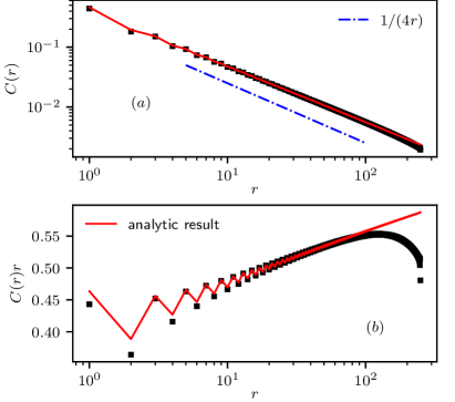
Figure 1: The spin-spin correlation function (7) (black squares) as a function of the spin separation $r$ for a chain of $L=500$ sites with open boundary conditions. The blue dashed line in (a) is the simple power-law decay $\sim r^{-1}$ . In (b) we plot $C(r)r$ to emphasize the logarithmic correction. The solid red line is the best fit to the analytical expectation (8) in both panels.

The leading terms of the correlation function $\left\langle\mathbf{S}_{i}\cdot\mathbf{S}_{i+r}\right\rangle$ in the regime $1\ll r\ll L$ are known to be (Lukyanov, 1998; Hikihara and Furusaki, 1998)

$$\left\langle\mathbf{S}_{i}\cdot\mathbf{S}_{i+r}\right\rangle=a\frac{A(r)}{r}+b\frac{(-1)^{r}}{r^{2}},$$ (8)

with $a=1$ and $b$ being an unknown constant (both of which we take as fitting parameters for our numerical data) and the function

$$A(r)=\frac{3}{\sqrt{8\pi^{3}g}}\left(1-\frac{3}{16}g^{2}+\frac{156\zeta(3)-73}{384}g^{3}+{\cal O}\left(g^{4}\right)\right),$$ (9)

where $\zeta\left(s\right)$ is the Riemann zeta function and $g\equiv g(r)$ is obtained from

$$g^{-1}+\frac{1}{2}\ln g=\ln\left(2\sqrt{2\pi}e^{\gamma+1}r\right),$$ (10)

where $\gamma$ is the Euler constant. In both panels of Fig. 1 we fit our numerical data to the analytical expectation (8) and find that $a=0.983(1)$ and $b=-0.452(9)$ (red solid line). Therefore, we confirm that, to leading order, $\left\langle\mathbf{S}_{i}\cdot\mathbf{S}_{i+r}\right\rangle\sim\sqrt{\ln r}/r$.

We now study the end-to-end correlation function. For large system sizes ($L\gg 1$), we expect that

$$C_{1,L}=\left\langle\mathbf{S}_{1}\cdot\mathbf{S}_{L}\right\rangle=c\frac{[\ln(L/L_{0})]^{\theta}}{L^{\eta_{s}}},$$ (11)

where the surface correlation function exponent $\eta_{s}=2x_{s}=2$ (Cardy, 1984; Alcaraz et al., 1987). For the same reason as in the bulk correlations, we expect a logarithmic factor. To the best of our knowledge, however, the exponent $\theta$ is unknown.

Figure 2(a) shows $C_{1,L}$ for system sizes ranging from $L=40$ up to $500$. Clearly, $C_{1,L}$ does not decay as a simple power law $\sim L^{-2}$. In Fig.  2(b) we plot $C_{1,L}L^{\eta_{s}}$, from which we fit Eq. (11) to our data taking $\theta$, $c$, and $L_{0}$ as fitting parameters. We obtain $L_{0}=0.7$(2), $c=1.5(3)$, and $\theta=1.5(2)$. Evidently, the value of the exponent $\theta\approx 1.5$ should be interpreted only as an effective exponent since we are not performing a thorough finite-size study.

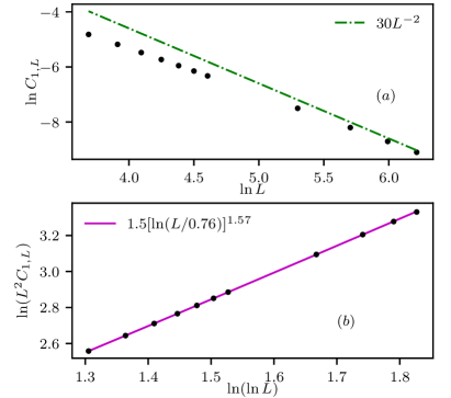
Figure 2: (a) The end-to-end correlation $C_{1,L}=\left\langle\mathbf{S}_{1}\cdot\mathbf{S}_{L}\right\rangle$ for system sizes ranging from $L=40$ to $L=500$. (b) Same data as in (a) with $C_{1,L}$ multiplied by $L^{2}$ in order to highlight the logarithmic prefactor [see Eq. (11)].

III.2 The disordered AF Heisenberg chain

In this section, we report our main results on the ground-state correlation function of the AF disordered Heisenberg chain [$\Delta=1$ in the Hamiltonian (1)] using the aDMRG method.

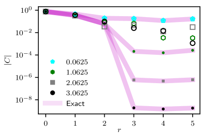
Figure 3: The ground-state spin-spin correlation (7) for a single disorder realization $\left\{J_{i}\right\}$ drawn from (6) for various disorder strengths $D$ (increased in steps by the aDMRG method) and system size $L=10$. The thick solid curve, open symbols, and solid symbols are, respectively, the values obtained using the exact diagonalization, the standard DMRG, and aDMRG methods.

As a benchmark, we start by computing the correlation function $C$ [as defined in Eq. (7)] for a single disorder realization of coupling constants $\{J_{i}\}$ using the exact diagonalization, the standard DRMG, and the aDMRG methods for a chain of $L=10$ spins. As shown in Fig. (3), the standard DMRG method fails to reproduce the exact values, while the aDMRG method reproduces the exact ones within a relative error smaller than $10^{-3}$. We have repeated this benchmark for dozens of other disorder realizations and have obtained the same result.

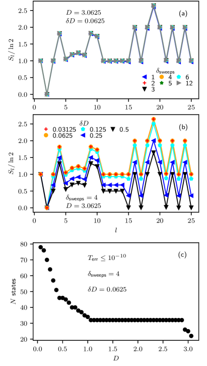
Figure 4: (a) and (b) The entanglement entropy ${\cal S}_{l}$ as a function of the system size $l$ [see Eq. (5)] for a single disorder realization of a chain of $50$ sites long and disorder parameter strength $D=3.0625$. The subsystem $A$ consists of all spins from sites $1$ to $l$. In (a), ${\cal S}_{l}$ is shown for different numbers of DMRG sweeps $\delta_{\text{sweeps}}$ used in the adaptive strategy while the disorder increment $\delta D$ is kept fix. In (b), ${\cal S}_{l}$ is shown for different values of $\delta D$ and fix $\delta_{\text{sweep}}$. (c) The total number of states $N$ needed to ensure that the DMRG truncation error is not larger than $T_{\text{err}}=10^{-10}$ as the disorder strength is increased.

In order to illustrate the convergence of the adaptive strategy, we plot in Fig. 4 an additional analysis with respect to the (a) number of DMRG sweeps $\delta_{\text{sweeps}}$ necessary for convergence when increasing the disorder strength from $D\rightarrow D+\delta D$, (b) the disorder strength increment $\delta D$, and (c) the number of states needed to keep the DMRG error truncation $T_{\text{err}}$ below a certain threshold. We then compute the entanglement entropy $S_{l}$ (5) as a function of the subsystem size $l$. Here, we show only a typical disorder realization of a chain $L=50$ sites long with final disorder strength $D=3.0625$, but we have checked the same quantitative results for other chain sizes. In Fig. 4(a), we see that $\delta_{\text{sweeps}}=2$ or $3$ is already enough to ensure convergence of ${\cal S}_{l}$ (and, presumably, of the state $\left|\psi_{D}\right\rangle$). In Fig. 4(b), we see that a small disorder parameter increment $\delta D\lessapprox 2^{-4}$ is necessary in order to obtain convergence. We notice that increasing the number of intermediate sweeps $\delta_{\text{sweeps}}$ does not improve convergence for larger $\delta D$’s. Finally, we plot in Fig. 4(c) the total number of states $N$ required to keep the DMRG truncation error below $T_{\text{err}}=10^{-10}$ as the disorder strength $D$ is increased along the adaptive strategy. Clearly, the disorder gets larger, fewer states are necessary. We report that the entanglement entropy ${\cal S}_{l}$ converges less rapidly than the correlation function $C$; that is, if the parameters used are enough to ensure the convergence of ${\cal S}_{l}$, then $C$ is also converged.

Now we turn to the main results of this work. The first one is on the mean value of the bulk correlations $\overline{C}(r)$ [as defined in (7)] for chains of $L=100$ spins and various disorder strengths $D$, shown in Fig. 5. In Fig. 5(a) we can see that $\overline{C}$ crosses over from the clean behavior $C_{\text{clean}}\sim(\sqrt{\ln r})/r$ (black solid line) to the disordered one $\overline{C}\sim r^{-2}$ (red dashed line) with increasing disorder strength $D$, as expected.

In order to obtain a data collapse, we now follow the reasoning of Ref. Getelina and Hoyos, 2020. The first step is to relate the clean-dirty crossover length $\xi_{D}$ to the multiplicative prefactor $c_{D}$ of the correlation function $\overline{C}=c_{D}r^{-2}$. This is accomplished by assuming a sharp crossover at $r=\xi_{D}$, i.e., $C_{\text{clean}}=A(\xi_{D})/\xi_{D}=\overline{C}=c_{D}/\xi_{D}^{2}$, and thus, $c_{D}\sim\xi_{D}A(\xi_{D})$, with $A(r)$ defined in (9). The second step is to rescale the spin-spin separation $r$ in terms of $\xi_{D}$ (i.e., $r\rightarrow r/\xi_{D}$) and to rescale $\overline{C}$ accordingly. Thus, $\overline{C}\xi_{D}/A(\xi_{D})\sim\left(r/\xi_{D}\right)^{-2}$. The third step is to relate $\overline{C}$ to the disorder strength $D$. As explained in the Introduction, the associated Lyapunov exponent is

$$\gamma_{D}\equiv\left[\text{var}\left(\ln J\right)\right]^{\frac{1}{3-2K}}.$$ (12)

with $2K=\left[1-\pi^{-1}\arccos\left(\Delta\right)\right]^{-1}$ (Doty and Fisher, 1992), and we ignore any possible multiplicative prefactor. As $\xi_{D}\propto\gamma_{D}^{-1}$, then, $\xi_{D}\propto D^{-1}$ for $\Delta=1$. In order to proceed, we need to take a final step: we assume that $A(\xi_{D})\approx 1$ for $D>1$. This is justified after we verify that $\xi_{D}$ is of order unity in the data in Fig. 5(a). While $A(\xi_{D})$ cannot be dropped for $D<1$, for our purposes we need the correct scaling function only in the strong-disorder regime. Thus, we plot $\left|\overline{C}\right|/D$ vs $rD$ in Fig. 5(b). The data collapse reasonably well apart from the deviations due to finite-size effects and $D$-dependent corrections to $A(\xi_{D})$ (or $c_{D}$) in the $D<1$ regime. Finally, in Fig. 5(c) we plot $\overline{C}Dr^{2}$ as a function of $rD$, which should be compared to the clean case in Fig. 1(b). The increasing of the plateau for the largest values of $D$ suggests the nonexistence of the logarithmic factor. Notice that this is reached only for the largest values of $D$. For $D\approx 2$, the plateau seems like a shoulder and is strongly affected by the finite-size corrections. As reported in Ref. Getelina and Hoyos, 2020, this can mimic logarithmic factors. We remark that the numerical observation of this plateau is not a simple task to accomplish even in the free-fermion case $\Delta=0$ with periodic boundary conditions (Getelina and Hoyos, 2020).

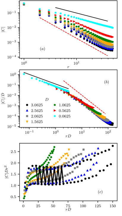
Figure 5: The mean value of the correlation function (7) of the AF Heisenberg chain for $L=100$ as a function of the spin-spin separation $r$ for various disorder strengths $D$. (a) shows the bare value of $\left|\overline{C}\right|$ as a function of the spin-spin separation $r$. In (b), we plot $\left|\overline{C}\right|/\gamma_{D}$ as a function of $\gamma_{D}r$ in order to obtain a data collapse [see arguments around Eq. (12)]. The black solid line is proportional to the clean correlation (8), and the red dashed line is proportional to $r^{-2}$. The data in (b) are replotted in (c) with the vertical axis multiplied by $\left(\gamma_{D}r\right)^{2}$. The solid line is a fit to Eq. (2).

We now extract the value of the exponent $\eta$ and the difference $c_{\text{o}}-c_{\text{e}}$ between the numerical prefactors. We then analyze the data in Fig. 5(b) excluding the points which, due to strong finite-size effects, are out of the data collapse. The resulting data points are replotted Fig. 6(a) from which we fit Eq. (2) to each data set using $\eta$, $c_{\text{o}}$, and $c_{\text{e}}$ as fitting parameters. The corresponding values are plotted in Fig. 6(b) as a function of the disorder strength $D$. For small values of $D$, $\eta$ is simply an effective exponent due to the large associated crossover length. As $D$ increases, the crossover length shortens, and the effective exponent $\eta$ approaches the expected value $\eta=2$. We observe analogous behavior for the difference $c_{\text{o}}-c_{\text{e}}$. The fitted values for $D=3.0625$ are $\eta=1.99(2)$ and $c_{\text{o}}-c_{\text{e}}=1.01(5)$. For completeness, we report that these values were obtained by fitting the data within the range $x_{\text{min}}\leq rD\leq x_{\text{max}}$ where $\left(x_{\text{min}},x_{\text{max}}\right)\approx\left(4,10\right)$, $\left(10,20\right),$ $\left(15,30\right)$, $\left(20,40\right)$, $\left(25,50\right)$, and $\left(25,60\right)$, for $D=0.5625,\,1.0625,\dots,\,3.0625$, respectively.

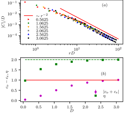
Figure 6: (a) Replot of the data in Fig. 5(b) excluding the data points which do not follow the data collapse. (b) The exponent $\eta$ and the difference $c_{\text{o}}-c_{\text{e}}$ obtained from the best fit of Eq. (2) to the data in (a) (see text).

We now study the mean end-to-end correlation $\overline{C_{1,L}}=-\overline{\left\langle\mathbf{S}_{1}\cdot\mathbf{S}_{L}\right\rangle}$ for even $L$. In Fig. 7(a), $\overline{C_{1,L}}$ is plotted as a function of the system size $L$ for various values of the disorder parameter $D$, including $D=0$ (the clean system) for comparison. Disregarding logarithmic corrections, $C_{1,L}\sim L^{-\eta_{s}(0)}$, with a clean surface exponent $\eta_{s}(0)=2$ that is greater than the bulk exponent $\eta=1$ (see Fig. 2). In the disordered case $D\neq 0$, however, $C_{1,L}\sim L^{-\eta_{s}(0)}$, with surface exponent $\eta_{s}(D\neq 0)=1$ (Fisher and Young, 1998), which is less than the bulk one $\eta(D\neq 0)=2$. In the SDRG framework, $C_{1,L}$ is proportional to the probability that the first and last spins form a singlet. Thus, on average, it decays with the system $\sim L^{-1}$. Our data (see Fig. 2) are clearly compatible with this prediction. We notice a nonmonotonic behavior of $C_{1.L}$ as a function of $D$. It increases from $D=0$ up to $D^{*}\approx 0.7(2)$ and diminishes for larger $D$. A similar behavior was also found in the free-fermion case $\Delta=0$ for the longitudinal correlation $\overline{C_{1,2}^{z}}$ (Getelina and Hoyos, 2020).

In order to highlight a possible logarithmic factor, we replot in Fig. 7(b) the data from Fig. 7(a) with $C_{1,L}$ multiplied by $L^{\eta_{s}(D)}$, with $\eta_{s}(D)=1+\delta_{D,0}$. In the clean case, $C_{1,L}$ clearly has a logarithmic multiplicative factor [as already reported in Fig. 2(b)]. In the disordered case, our data are compatible with its absence. Even for the smallest value of disorder $D=1/16$, the corresponding value of $\eta_{s}\approx 1.1$ is already far from the clean value $2$. This indicates that the end-to-end correlation is less affected by the clean-dirty crossover when compared to the bulk correlations. More interestingly, the logarithmic factor (if any) is strongly affected by disorder indicating its absence.

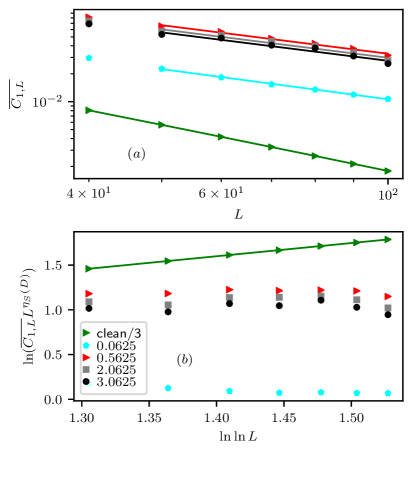
Figure 7: (a) The average end-to-end correlation $\overline{C_{1,L}}=-\overline{\left\langle\mathbf{S}_{1}\cdot\mathbf{S}_{L}\right\rangle}$ of the AF Heisenberg chain as a function of the system size and for various values of the disorder parameter $D$. The straight lines are power-law fits to $aL^{-\eta_{s}}$ from which we obtain $\eta_{s}=1.02(7)$ for all values of $D$ except for $D=1/16$, in which $\eta_{s}=1.1$. In the clean case, however, the solid line is the fit to Eq. (11) already reported in Fig. 2. (b) A replot of data in (a) with $\overline{C_{1,L}}$ multiplied by $L^{\eta_{s}(D)}$, with $\eta_{s}(D)=1+\delta_{D,0}$. The solid line is the same in Fig. 2(b). For an easier comparison, in panel (b) we have divided $C_{1,L}$ by a factor of 3 in the clean case.

We now turn our attention to the typical value of the correlation function,

$$C_{\text{typ}}=\exp\left(\overline{\frac{\sum_{i=L/4}^{3L/4-r}\ln\left|\langle\mathbf{S}_{i}\cdot\mathbf{S}_{i+r}\rangle\right|}{L/2-r}}\right),$$ (13)

which is defined analogously to Eq. (7). This quantity is plotted in Fig. 8 as a function of the spin-spin separation $r$ for $L=100$ and various values of $D$. Figure 8(a) shows $\ln C_{\text{typ}}$ vs $\sqrt{r}$, from which the linear behavior (3) is confirmed for $\xi_{D}\ll r\ll L$.

Analogously to the average value (see Fig. 5), we produce a data collapse based on Eq. (3). This is done by fitting Eq. (3) to the data in Fig. 8(a) in a region which, presumably, is weakly affected by finite size (see magenta lines). The resulting collapsed data are shown in Fig. 8(b). The fitting parameters $A$ and $c_{D}$ are shown in Fig. 8(c) as a function of the disorder parameter $D$. In agreement with Eq. (3), $A$ is disorder independent for large $D$. We attribute the weak $D$ dependence to the large crossover length in the weak disorder limit. Similar behavior was found in the free-fermion case $\Delta=0$ (Getelina and Hoyos, 2020).

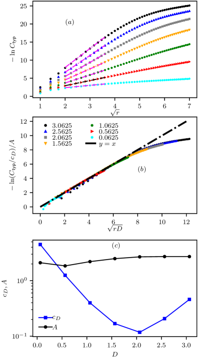
Figure 8: (a) The typical correlation function (13) of the AF Heisenberg chain for $L=100$ and different values of the disorder strength $D$. The magenta lines are the best fits to Eq. (3), from which the data collapse in (b) is produced. (c) The values of the fitting parameters $A$ and $c_{D}$ as a function of the disorder parameter $D$.

Finally, we now study the distribution of spin-spin correlations. We restrain ourselves to the quantity $C=\left|\left\langle\mathbf{S}_{L/4}\cdot\mathbf{S}_{3L/4}\right\rangle\right|$ for chains of size $L=100$ and many values of $D$. In Fig. 9(a) we plot the distribution of $-\ln\left(C/c_{D}\right)/\left(A\sqrt{\gamma_{D}r}\right)$, with $r=L/2$ and $A$ and $c_{D}$ being the fitted values in Fig. 8(c). The data collapse for the largest values of $D$ confirms the conjecture of Ref. Fisher, 1994 which states that the distribution of $-\ln\left|C_{i,j}\right|/\sqrt{\left|i-j\right|}$ converges to a nontrivial distribution for large spin-spin separation $\left|i-j\right|\gg 1$. Here, in addition, we conclude that $\ln\left|C_{i,j}\right|/\sqrt{\gamma_{D}\left|i-j\right|}$ converges to a nontrivial, narrow, and universal (disorder-independent) distribution for $\gamma_{D}\left|i-j\right|\gg 1$. The same observation was reported in the free-fermion case $\Delta=0$ (Getelina and Hoyos, 2020).

We are now interested in the functional form of this nontrivial distribution. We thus study the distribution of $w=\frac{\overline{\ln C}-\ln C}{\sigma_{\ln C}}$ (with $\sigma_{x}^{2}=\overline{x^{2}}-\overline{x}^{2}$ being the variance of $x$), which is shown in Fig. 9(b).

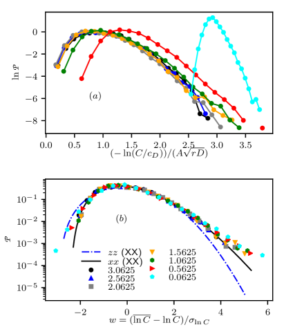
Figure 9: Normalized histogram of the correlation function $C=\left|\left\langle\mathbf{S}_{L/4}\cdot\mathbf{S}_{3L/4}\right\rangle\right|$. In (a), it is rescaled by the parameters $A$ and $c_{D}$ [see Eq. (3)] given in Fig. 8(c). (b) shows the same data rescaled by its average and standard deviation. The solid black line is a fit to Eq. (14) (see text). The histogram was built using $2\times 10^{4}$ distinct disorder configurations of coupling constants $\left\{J_{i}\right\}$. The blue dashed and black solid lines are, respectively, the associated distributions for the XX chain [$\Delta=0$ in (2)] for the longitudinal $C^{z}$ and transverse $C^{x}$ spin-spin correlations.

In Ref. Getelina and Hoyos, 2020, the distributions of the transverse ($C^{x}$) and longitudinal ($C^{z}$) correlations for the XX model [$\Delta=0$ in Eq. (1)] were shown to be well fitted by

$${\cal P}(w)=B\exp\left\{-\left|\frac{w-w_{1}}{\delta_{1}}\right|^{\gamma_{1}}-\left(\frac{\delta_{2}}{w-w_{2}}\right)^{\gamma_{2}}\right\}.$$ (14)

The first term in the exponential dictates the weak-correlation behavior $w\gg 1$, which, naively, is expected to be a Gaussian; that is, $\gamma_{1}$ is expected to be $2$. Thus, $w_{1}$ and $\delta_{1}$ are, respectively, the associated mean and width. The second term in the exponential dictates the strong-correlation regime. A sharp cutoff, represented by $\omega_{2}$, is expected since the correlations $C_{i,j}$ cannot be arbitrarily large in absolute value. Thus, $w>w_{2}$. The parameters $\delta_{2}$ and $\gamma_{2}$ are the associated width and exponent, respectively. The parameter $B$ is just the normalization. The fitted values in that work for the transverse correlations are $\delta_{1}=1.66$, $\delta_{2}=79$, $w_{1}=-1.45$, $w_{2}=-2.51$, $\gamma_{1}=1.71$, and $\gamma_{2}=0.41$, which is plotted as a black solid line in Fig. 9(b). Surprisingly, it fits our data quite satisfactorily. It is thus tempting to conjecture that the distribution of the transverse correlation in the model Hamiltonian (1) is $\Delta$ independent in the infinite-randomness regime $-\frac{1}{2}<\Delta\leq 1$. For comparison, we also plot the distribution of the longitudinal correlations $C^{z}$ (blue dashed line) of the XX model obtained in Ref. Getelina and Hoyos, 2020.

Thus, we conclude that the distribution of $\ln\left|C_{i,j}^{x}\right|/\sqrt{\gamma_{D}\left|i-j\right|}$ in the long-distance regime $\gamma_{D}\left|i-j\right|\gg 1$ converges to a nontrivial distribution which is narrow, universal (disorder independent), and possibly $\Delta$ independent. The same conclusions apply for the distribution of longitudinal correlations, except that it is $\Delta$ dependent.

IV Conclusions and discussion

In this work, we have studied various measures of the ground-state spin-spin correlations $C_{i,j}=\left\langle\mathbf{S}_{i}\cdot\mathbf{S}_{j}\right\rangle$ of the AF spin-$1/2$ Heisenberg chain [$\Delta=1$ in Eq. (1)] with random coupling constants. We applied the recently developed (Xavier et al., 2018) adaptive strategy, which enabled us to study strongly (quenched) disordered systems using the unbiased DMRG method.

Our data are entirely compatible with the SDRG analytical predictions (Fisher, 1994; Hoyos et al., 2007b). Specifically, regarding the bulk correlations (2) in the regime $1\ll\gamma_{D}\left|i-j\right|\ll L$, we verified that the exponent $\eta=2$ and prefactor difference $c_{\text{o}}-c_{\text{e}}=1$ are universal (disorder independent). Our data confirm that the typical value of the correlations [Eq. (3)] decay stretched exponentially with the spin-spin separation with universal exponent $\psi=1/2$. Furthermore, we have confirmed the observation of Ref. Laflorencie et al., 2004 that the relevant length scale is the inverse Lyapunov exponent $\gamma_{D}$ in Eq. (12), which plays the role of the clean-dirty crossover length. This observation was made precise in the XX chain case ($\Delta=0$). In that case, this length scale is the inverse of the Lyapunov exponent of a single-parameter theory of the associated free-fermion system with particle-hole symmetry (Mard et al., 2014). We have also studied the distribution of the spin-spin correlations for a fixed distance and confirmed the conjecture of Ref. Fisher, 1994 that $\ln\left|C_{i,j}\right|/\sqrt{\left|i-j\right|}$ converges to a nontrivial distribution for $\left|i-j\right|\gg 1$. We have also studied the mean value of the end-to-end correlations $C_{1,L}$ and confirmed that it decays $\sim L^{-\eta_{s}}$ with universal surface exponent $\eta_{s}=1$ (Fisher and Young, 1998). All these results were thoroughly confirmed by many others using different methods (Iglói and Monthus, 2005, 2018).

Let us now summarize our new findings. The first one is in regard to the end-to-end correlations on the clean system. Our data are compatible with the predicted surface exponent $\eta_{s}=2$. In addition, we showed the existence of a logarithmic correction with effective exponent $\theta=1.5(1)$ [see Eq. (11)]. In the presence of disorder, this logarithm correction disappears. With respect to the distribution of correlations, we have found that the distribution of $\ln\left|C_{i,j}\right|/\sqrt{\gamma_{D}\left|i-j\right|}$ converges to a nontrivial, narrow, and universal distribution for $\gamma_{D}\left|i-j\right|\gg 1$. We have also found that, within our statistical precision, it is equal to that of the transverse correlations of the XX chain reported in Ref. (Getelina and Hoyos, 2020). It is thus tempting to conjecture that, besides being nontrivial, narrow, and universal, the distribution of $\ln\left|C_{i,j}^{x}\right|/\sqrt{\gamma_{D}\left|i-j\right|}$ does not depend (or depends weakly) on $\Delta$.

One reported result that we have not confirmed is the logarithmic factor on the mean correlations of the disordered chain (Shu et al., 2016). As we have shown, our data are compatible with its absence in both the mean (see Figs. 5 and 6) and typical (see Fig. 8) values of the bulk correlations, as well as in the mean value of the end-to-end correlation (see Fig. 7). Evidently, we cannot exclude (although it very implausible) a logarithmic factor appearing for system sizes larger than the ones studied here. If that is the case, we recall that the adaptive DMRG method employed here starts with the near-clean wave function, which does have a logarithmic factor in its two-point correlation. The fact that we do not detect it when the disorder strength is increased strongly suggests that the origin of the logarithmic factor, if one exists, is unrelated to that of the clean system.

Currently, it is unclear why the zero-temperature quantum Monte Carlo study of Ref. Shu et al., 2016 predicts a logarithmic correction. The only suggestion that comes to us is finite-size effects. As shown in Fig. 5(c), the finite-size corrections are still strong for $D\approx 2$ even for system sizes $L\approx 100$. More importantly, the finite-size correction promotes a slow increase in the correlations which can be interpreted as a logarithmic correction (Getelina and Hoyos, 2020). Interestingly, $D=2$ is the strongest disorder parameter value studied in Ref. Shu et al., 2016. However, those authors considered periodic boundary conditions where finite-size effects are presumably smaller. In addition, they were able to study chains with sizes larger than ours.

Finally, we would like to point out that logarithmic factors are predicted by the SDRG method. They appear in the susceptibility and specific heat of infinite-randomness critical chains (but not in the correlations) (Fisher, 1994) and in certain quantities of critical chains at a Kosterlitz-Thouless like transition (Altman et al., 2004; Vojta et al., 2011; Juhász et al., 2014). Interestingly, logarithmic factors appear in the correlations of the clean Heisenberg chain ($\Delta=1$) and in the weakly disordered XXZ chain at the point $\Delta=-\frac{1}{2}$. In both cases, the associated renormalization-group flow is of the Kosterlitz-Thouless type (Ristivojevic et al., 2012).

In conclusion, our numerical results are in agreement with those predicted by the SDRG method, which, presumably, yields asymptotically exact results for the ground-state properties of the model Hamiltonian (1) in the parameter region $-\frac{1}{2}<\Delta\leq 1$. We have also shown that the adaptive DMRG method is capable of tackling one-dimensional disordered systems. It can be easily implemented using the standard DMRG method without much more coding effort, and therefore, it adds to the toolbox of unbiased theoretical methods for disordered systems.