Practical Quantum State Tomography for Gibbs states

Abstract

Quantum state tomography is an essential tool for the characterization and verification of quantum states. However, as it cannot be directly applied to systems with more than a few qubits, efficient tomography of larger states on mid-sized quantum devices remains an important challenge in quantum computing. We develop a tomography approach that requires moderate computational and quantum resources for the tomography of states that can be approximated by Gibbs states of local Hamiltonians. The proposed method, Hamiltonian Learning Tomography, uses a Hamiltonian learning algorithm to get a parametrized ansatz for the Gibbs Hamiltonian, and optimizes it with respect to the results of local measurements. We demonstrate the utility of this method with a high fidelity reconstruction of the density matrix of 4 to 10 qubits in a Gibbs state of the transverse-field Ising model, in numerical simulations as well as in experiments on IBM Quantum superconducting devices accessed via the cloud. Code implementation of the our method is freely available as an open source software in Python.

I Introduction

Quantum State Tomography (QST) is the process of reconstructing the density matrix of a quantum state by measuring multiple copies of it [1]. QST is a useful tool for the characterization and verification of quantum hardware, and can also be used for understanding fundamental properties of a system such as entanglement [2, 3]. There exist several well-established QST methods, which have been implemented on many types of devices and setups [4, 5, 6, 7, 8]. However, the number of measurements required in common QST methods, such as maximum likelihood estimation, grows exponentially with the number of qubits in the system [9, 10], rendering these methods infeasible for systems with more than a few qubits. There are several approaches to reduce the number of measurements needed for QST, either by making assumptions on the quantum state  [11, 12, 13, 14, 15], by circumventing the need to reconstruct the full density matrix [16, 17] or by making adaptive measurement process [18].

An important class of quantum states in condensed matter physics and quantum computing are Gibbs states of local Hamiltonians. These are states $\rho$ that can be parametrized as

$$\rho=\frac{1}{Z}e^{-H},$$ (1)

where $Z$ is an overall normalization factor, and $H$, called the Gibbs Hamiltonian (GH), is (at least approximately) a $k$-local operator; namely, $H$ is a sum of terms that act non-trivially on $k$ spatially contiguous degrees of freedom according to the connectivity topology of some relevant system. Gibbs states describe the equilibrium properties of many-body quantum systems [19], and as such are expected to approximately describe the dynamics of systems that thermalize due to a coupling with a bath [20], as well as subsystems of closed systems that thermalize under their own dynamics [21, 22]. They are also used as a model (quantum Boltzmann machine) in quantum machine learning [23], and their preparation is an essential part of various quantum algorithms [24, 25]. Thus, states that can be approximately described as Gibbs states ubiquitously arise in quantum simulations of many-body systems and when quantum algorithms are implemented on noisy devices.

In this work we introduce a practical tomography approach for approximate Gibbs states that we call Hamiltonian Learning Tomography (HLT). Our main idea is to use the Hamiltonian learning algorithm of Ref. [26] to efficiently identify a restricted ansatz for the Gibbs Hamiltonian, described by a small number of relevant parameters. Then, following the proposal of Entanglement Hamiltonian Tomography (EHT) from Ref. [27], and employing improvements important in our context, the ansatz is optimized with respect to the results of local measurements. Adapting elements from these two methods allows us to significantly extend the scopes in which they can be used and overcome drawbacks in each of them. All of this is achieved while using moderate computational and quantum resources.

As we will show, the use of the Hamiltonian learning algorithm to generate an ansatz removes the need for an a-priori knowledge of the Hamiltonian that parametrizes the state, as relied upon in EHT. Moreover, the Hamiltonian learning ansatz turns out to require a very low number of measurements for reaching a high tomography precision, in comparison with traditional QST. At the same time, using an optimization similar to that of EHT fixes the main drawbacks of the Hamiltonian learning procedure of Ref. [26], as we in explain in Sec. III.

To demonstrate the potential of our approach as a practical tool for characterizing the state of mid-sized quantum devices, we study it in detail using both numerical simulations and experiments on actual quantum hardware. We obtain a high fidelity of reconstruction of the density matrix of 4 to 10 qubits on an IBM Quantum superconducting device accessed via the cloud [28]. Using a variational algorithm to create the Gibbs state of a 1D transverse-field Ising Hamiltonian, we observe fidelities of over $0.99$ in a system of 5 qubits using only fifty thousand measurements, while a traditional QST reaches in our experiments fidelities of less than $0.6$ using the same number of measurements (and about five million measurements are required for a reliable result). For more than 5 qubits, the density matrix cannot be obtained at all with brute-force methods. Therefore, as an independent verification of the density matrix reconstructed using our tomography approach for 6 to 10 qubits, we use QST to directly measure subsystem reduced density matrices of 3 qubits, for all of which we observe a fidelity of over $0.99$ with the corresponding subsystem states of the full HLT density matrix. Finally, Greenberger-Horne-Zeilinger (GHZ) [29] states (also known as cat states) on quantum hardware are presented as a test case where we can detect performance issues with our method.

An open source Python code implementation of our method is freely available for the community on Github [30].

The structure of this paper is a follows; We start by giving a general review of the previous methods in Sec. II. In Sec. III we describe our method, and the states that fit into it. Then, results from simulations and quantum hardware demonstrating the method, are presented in Sec. IV. We conclude with a discussion and outlook in Sec. V.

II Background

II.1.   Entanglement Hamiltonian Tomography

Recently, in Refs.[31, 27, 32], a method called Entanglement Hamiltonian Tomography was suggested for the tomography of states generated by local Hamiltonians. Given a certain region in a many-body quantum system, its reduced density matrix encodes the results of all possible measurements in that region. Instead of learning this density matrix directly, one opts to learn the entanglement Hamiltonian, sometimes called modular Hamiltonian, defined by:

$$H_{E}\stackrel{{\scriptstyle\mathrm{def}}}{{=}}-\ln\left(\rho\right),$$ (2)

where $\rho$ is the reduced density matrix, and hence Eq. (2) takes formally the same expression as Eq. (1).

There are certain rigorous results, based on conformal field theory [33] and the Bisognano Wichmann theorem [34, 35, 36], that guarantee the locality of the entanglement Hamiltonian in various settings. These apply for ground states and for quantum quenches to a critical point of local Hamiltonians. The EHT method heuristically builds on these results, which formally apply for continuous, infinite and Lorentz invariant systems, and applies them to discrete lattice systems and to time evolution. It suggests an ansatz, based on these results, for the entanglement Hamiltonian, which is a linear combination of the terms of the underlying dynamical Hamiltonian. Given a Hamiltonian that is a sum of local terms $H=\sum_{i}h_{i}$, the basic ansatz consists of the same terms, but with arbitrary variational coefficients:

$$H_{E} =\sum_{i}\theta_{i}h_{i}, \theta_{i} \in\mathbb{R}.$$

The above ansatz can be further extended using physically motivated terms (such as momentum terms). The vector of parameters $\bm{\theta}$ is then optimized by sampling $\rho$ in several bases of rotated product states, which are defined by random local unitaries that form a $2$-design. The statistics of these measurements is then used to find $\bm{\theta}$ using a cost function and gradient based optimization methods (see Sec. III.2).

II.2.   Hamiltonian learning using a constraint matrix

Quantum Hamiltonian learning is the problem of reconstructing a Hamiltonian by measuring its dynamics [37, 38, 39, 40, 41, 42, 43, 44, 45] or a steady state of the dynamics  [46, 47, 48, 49, 50, 51]. A recent method for learning local Hamiltonians from steady states using local measurements [26] can be applied for the learning of Gibbs states of local Hamiltonians. Given many copies of a Gibbs state $\rho=\frac{1}{Z}e^{-H}$, we aim at learning the Gibbs Hamiltonian $H$, instead of learning $\rho$ directly. The method begins by noting that $[H,\rho]=0$ and therefore for every operator $A$,

$${\langle{i[A,H]}\rangle}_{\rho}\stackrel{{\scriptstyle\mathrm{def}}}{{=}}i\operatorname*{Tr}([A,H]\rho)=i\operatorname*{Tr}(A[H,\rho])=0,$$ (3)

where we used the cyclicity of the trace. Assuming $H$ is a $k$-local Hamiltonian, we first expand it in terms of a basis of $k$-local operators $\{S_{m}\}_{m=1}^{M}$, which we conveniently choose to be $k$-local Pauli operators (since the normalization factor $Z$ of Eq. (1) can absorb the identity component of $H$, we can assume without loss of generality that $H$ is traceless). Then

$$H=\sum_{m=1}^{M}v_{m}S_{m},$$ (4)

and our task is to estimate the coefficients $\{v_{m}\}$. Choosing a set of local “constraint operators” $\{A_{q}\}_{q=1}^{Q}$, where $Q\geq M$, we use Eq. (3) to obtain a linear constraint on $\{v_{m}\}$ for each $A_{q}$;

$${\langle{i[A_{q},H]}\rangle}_{\rho}=\sum_{m}{\langle{i[A_{q},S_{m}]}\rangle}_{\rho}v_{m}=0.$$ (5)

This set of equations can be compactly written as a matrix equation for the vector $\bm{v}\stackrel{{\scriptstyle\mathrm{def}}}{{=}}\{v_{m}\}$,

$$K\bm{v}=0,\qquad K_{q,m}\equiv\left<i\left[A_{q},S_{m}\right]\right>_{\rho},$$ (6)

where $K$ is a $Q\times M$ real matrix, which we call the constraint matrix (CM). As it is a homogenous equation, solving it gives $\bm{v}$ up to an overall factor. In order to have more equations than unknown (i.e., $Q>M$), we take the set of constraint operators to be all $(k+1)$-local Paulis.

The CM $K$ can be measured directly, as each of its entries is an expectation value of at most a $2k$-local Pauli. However, any finite number of measurement will necessarily produce statistical errors in the measured CM:

$$\tilde{K} =K+\epsilon E, \epsilon =O(1/\sqrt{m}).$$ (7)

Above, $\epsilon E$ is the statistical noise from the measurements, and we have distinguished for clarity a formal parameter $\epsilon$ that models the standard deviation of statistical noise, which depends on the number of measurements $m$. Consequently, the equation $\tilde{K}\bm{v}=0$ will generally not have a solution, and instead we will look for a $\bm{v}$ that minimizes $\|\tilde{K}\bm{v}\|$. This is precisely the smallest right singular vector (SV) of $\tilde{K}$, which will deviate from being proportional to the GH because of the noise. As shown in Ref. [26] using a perturbative analysis, the error in $\bm{v}$ due to the statistical noise depends on the singular values of $K$:

$$\mathbb{E}(\left\|\bm{v}-\bm{v}_{true}\right\|)\approx\epsilon\sqrt{\sum_{i>0}\frac{1}{\lambda_{i}}}+O(\epsilon^{2}),$$ (8)

where $\bm{v}_{true}$ is the exact coefficients vector of the Hamiltonian, and $\lambda_{i}$ are the eigenvalues of $K^{T}K$. Therefore, a sufficiently large gap between $\lambda_{1}$, the second smallest singular value of $K$, and $\lambda_{0}=0$ is an necessary condition for the CM method to work with a reasonable number of measurements.

III Hamiltonian Learning Tomography

III.1.   Description of the algorithm

In this section, we show how we can combine the Hamiltonian learning algorithm together with EHT, and introduce the Hamiltonian Learning Tomography (HLT) method.

To understand the general idea behind it, consider the expansion in Eq. (4), which defines a vector $\bm{v}$ for any Hamiltonian $H$ via the $k$-local Pauli basis. This expansion also defines a Hamiltonian $H_{\bm{v}}$ for every vector $\bm{v}$. Then by the definition of the $K$ matrix in Eqs. (5, 6), it follows that for every vector $\bm{v}$, the norm $\left\|K\bm{v}\right\|$ measures the commutativity of $H_{\bm{v}}$ with $\rho$. When $K$ is slightly perturbed, the Hamiltonians that correspond to its lowest singular values will be the ones that nearly commute with $\rho$, and so it is plausible that the actual Gibbs Hamiltonian is well approximated by a superposition of these Hamiltonians.

This intuition can be justified using perturbation theory, as shown in Appendix A. Indeed, considering Eq. (7) perturbatively in $\epsilon$, the lowest singular vector of $K$ will be a equal to the lowest singular vector of $\tilde{K}$ plus a first order correction, which is a superposition of the other singular vectors of $\tilde{K}$. The higher the singular value is, the smaller is the weight of the corresponding vector in the super position. Specifically, we show in Appendix A that if $\bm{v}_{0}$ is the zero singular vector of $K$ that corresponds to the exact Hamiltonian, and $\tilde{\bm{c}}_{l}$ is the projection of this vector on the subspace of the first $l$ singular vectors of the noisy $\tilde{K}$, then

$$\mathbb{E}\big{(}\left\|\tilde{\bm{c}}_{l}-\bm{v}_{0}\right\|^{2}\big{)}=\epsilon^{2}\sum_{i\geq l}\frac{1}{\lambda^{2}_{i}}+O(\epsilon^{3}),$$ (9)

where $\epsilon$ is the statistical noise parameter from Eq. (7) and the averaging $\mathbb{E}(\cdot)$ is defined with respect to the underlying probability space in which $E$ is defined.

Taking the lowest $l$ right singular vectors of $\tilde{K}$, we can now follow the EHT method to find the actual coefficients in the expansion of the actual GH. Formally, we define a $k$-local HLT algorithm with cutoff $l$ to consist of the following steps:

1. For a given (unknown) state $\rho$ prepared on a quantum device, measure all $2k$-local Paulis expectation values.

2. Construct a constraint matrix $\tilde{K}$ as described in Sec. II.2 with $k$-local Paulis as $\left\{S_{m}\right\}$ and $\left(k+1\right)$-local Paulis as $\left\{A_{q}\right\}$, and find its $l$ lowest singular vectors $\{\tilde{\bm{v}}^{(i)}\}_{i=1}^{l}$.

3. Define an ansatz for the GH using the above $l$ vectors and use them to introduce the variational parameters $\bm{\theta}$,

   $$H(\bm{\theta})=\sum_{i=1}^{l}\theta_{i}\Big{(}\sum_{m}\tilde{v}^{(i)}_{m}S_{m}\Big{)},$$ (10)

   and optimize $\bm{\theta}$ using a measurement-based loss function (see Sec. III.2).

For a fixed $k$, the number of $k$-local Paulis scales linearly in the size of the system. Therefore, the size of the CM and the number of its singular values are also linear in the number of qubits, which gives a polynomial description of the underlying Gibbs state.

Using the fact that the $k$-local Paulis from step (i) sit on contiguous sites, we can measure many of these observables simultaneously using the so-called overlapping local tomography technique introduced in Ref. [52]. This allows us to use $m$ global measurements to estimate every $t$-local observable using $m/3^{t}$ measurement results for $t=1,\ldots,2k$ — see Appendix C for more details. Finally, the same measurement results that were used in step (i) can be conveniently reused in step (iii) at the optimization step.

At this point, the reader may wonder why use only $l$ SVs out of all the possible SVs (e.g. $12N-9$ in case of $k=2$ and $1D$ chain). The reason is that limiting $l$ leads to a much more efficient optimization and might ease the convergence of gradient-based methods as a result of lower dimensionality [53, 54, 55]. Additionally, the complexity of each gradient computation, e.g., for the optimization algorithm from Ref. [56], scales linearly with the number of parameters. Moving to larger systems, this is even more pronounced. For example, an optimization with $10$ qubits using $30$ SVs required a few hours on a personal computer in our case, while using all the SVs may take up to several days. This saving in optimization time might become crucial when one wants to perform tomography many times.

III.2.   Ansatz Optimization

Once the $l$ singular vectors $\tilde{\bm{v}}^{(i)}$ of $\tilde{K}$ with the smallest singular values are found (see Sec. III), we need to optimize their corresponding weights. Specifically, we want to find the weights $\bm{\theta}$ such that the state $\rho(\bm{\theta})=\frac{1}{Z}e^{-H(\bm{\theta})}$, with $H(\bm{\theta})$ defined in (10), will match the measurements results. To that end, we use the loss function defined by

$$\chi^{2}(\bm{\theta})=\sum_{B}\sum_{\bm{s}}\left[P_{B}\left(\bm{s}\right)-\left\langle\bm{s}\right|U_{B}^{\dagger}\rho_{A}(\bm{\theta})U_{B}\left|\bm{s}\right\rangle\right]^{2}.$$ (11)

The first summation is over the $2k$-local Pauli bases needed for the construction of the constraint matrix (see Appendix C). $P_{B}(\bm{s})$ is the empirical probability to measure the bitstring $\bm{s}$ in the Pauli basis $B$, which was obtained from the experiment, and $\left\langle\bm{s}\right|U_{B}^{\dagger}\rho_{A}(\bm{\theta})U_{B}\left|\bm{s}\right\rangle$ is the corresponding probability from the ansatz. $U_{B}$ is a unitary that rotates the computational basis to the $B$ basis. The second summation is over all the possible string outcomes of $N$ qubits measurements.

Our loss function is different from the one used in Ref. [27] in that we do not use random unitaries for $U_{B}$. This is advantageous for HLT since it allows one to use the same measurements for both the calculation of the CM $\tilde{K}$ and the optimization. This choice is justified by the fact that $2k$-local Paulis are tomographically complete, meaning they form a basis of $2k$-qubits density matrices. Assuming that the underlying state we learn is described by a $k$-local GH, this means that when the loss function vanishes, the underlying state has the same $2k$-local reduced density matrices as the ansatz state $\rho(\bm{\theta})$. By Ref. [57], this implies that the two states are globally equal. Therefore, minimizing the loss function, using only Paulis basis measurements, is enough.

III.3.   Assessing the HLT performance

A non-trivial question is how to assess the performance of the HLT method in an actual experiment; how can we tell how close is the HLT-recovered state to the actual state in the hardware? We suggest two practical checks that can be performed. First, by doing local tomography of subsystems with a number of qubits that is larger than $k$ but feasible for QST, and checking that the resultant reduced density matrices are close to the corresponding reduced density matrices of the HLT state. Secondly, one can check how well the HLT state converges as a function of $l,m$, by calculating the fidelity of the state that was obtained with the highest $l,m$ with states of lower $l,m$. As we demonstrate in Sec. IV.2 (Fig. 6 bottom), fast convergence indicates a better performance of HLT.

IV Results

In this section we present our results, which demonstrate the usage and performance of HLT on two cases: a chain of $N$ qubits with either a 1D transverse Ising model Gibbs state, or the reduced density matrix of a GHZ state. As we show in Sec. IV.2, the latter is a Gibbs state of the classical Ising model at $T=0$. In both cases, $k=2$. We present both numerical simulations results and results of IBM Quantum devices accessed via the cloud [28], implemented using the Qiskit framework [58]. Simulations and data processing were done on a personal computer with $32$Gb RAM memory. To assess the quality of our method, we use the quantum fidelity, defined by $F(\rho,\sigma)\stackrel{{\scriptstyle\mathrm{def}}}{{=}}(\operatorname*{Tr}\sqrt{\sqrt{\rho}\sigma\sqrt{\rho}})^{2}$ [59, 60].

When running HLT with $m$ measurements, those were distributed equally between the $3^{2k}$ basis-measurements that were needed to measure the expectation values of $2k$-local Paulis (see Sec. III and Appendix C). On the other hand, when $m$ measurements were used for ordinary QST on $N$ qubits, the measurements were distributed equally between the $3^{N}$ measurement bases. More details on the QST procedure can be found in Appendix D. When all SVs were used for HLT, $l$ is denoted by $l_{max}$.

In our analysis, the optimization was done using SciPy’s [61] nonlinear least-squares solver (with 2-point Jacobian computation method) which uses the algorithm from Ref. [56]. We also implemented gradient decent optimization method (using the same loss function) with PyTorch [62] and were able to reproduce the results from the first optimization method, validating the optimization results.

IV.1.   Transverse Ising Gibbs States

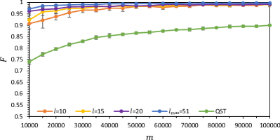
Figure 1: Results of a numerical simulation checking the HLT performance on an exact Gibbs state of the Transverse Ising model on 5 qubits with $k_{B}T=1$. The plot shows the fidelity between the exact Gibbs state and the HLT-reconstructed state as a function of the total number of measurements ($m$) for different numbers of singular values ($l$). The green line shows the fidelity of the exact state with a QST-reconstructed state using $m$ measurements. The plot shows the clear advantage of the HLT approach in this case. Results are averaged over $10$ simulation runs, error bars calculated using standard deviation.

a)

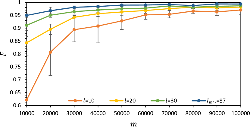
b)

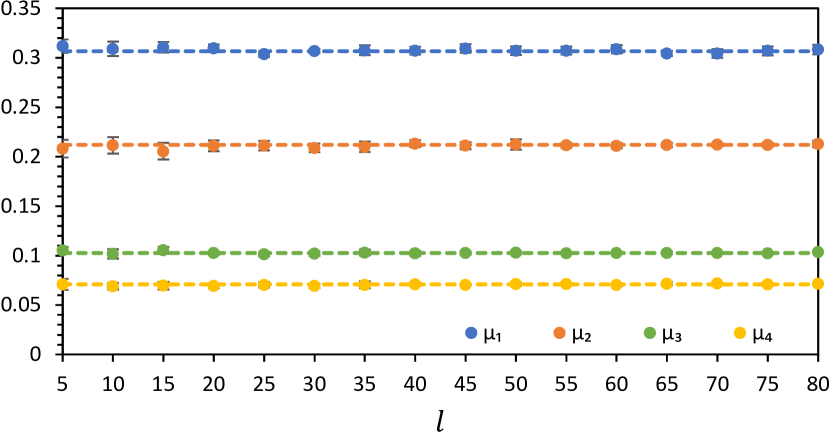
Figure 2: Numerical simulation results of HLT of an exact Gibbs state of $8$ qubits for the transverse-field Ising model. Results are averaged over $10$ simulation runs, error bars calculated using standard deviation. a) Fidelity between the exact Gibbs state and HLT-reconstructed state as a function of the number of measurements ($m$), for different numbers of singular values ($l$). b) The performance of HLT on non-local, non-linear quantities. The plot shows the four highest eigenvalues $\mu_{i}$ of the HLT-reconstructed state with $m=10^{5}$ as a function of the number of singular values ($l$). Dashed lines denote the exact eigenvalues of the Gibbs state. The plot shows excellent reconstruction around $l\gtrsim 20$.

The 1D Transverse Ising Hamiltonian is given by:

$$H_{TI}=\sum_{\left<i,j\right>}X_{i}X_{j}+\sum_{i}Z_{i}.$$ (12)

In this section, we study the case $k_{B}T=1$, which leads to the Gibbs state:

$$\rho_{TI} =\frac{1}{Z}e^{-H_{TI}}, Z =\operatorname*{Tr}\left(e^{-H_{TI}}\right).$$ (13)

IV.1.1.   Exact Gibbs state simulations

We first studied the performance of HLT in numerical simulations of an exact Gibbs state of the transverse-field Ising model. We started with a $5$ qubits state, and simulated the HLT protocol on it using $l=10,15,20$ and $l_{max}=51$ SVs and a total number of measurements that was varied from $m=5,000$ to $m=10^{5}$. For comparison, we also performed a traditional QST using the same number of measurements (but with different measurement bases — see Appendix D ). Our results are shown in Fig. 1, where the fidelities of the different protocols with the exact Gibbs state are plotted. The plot clearly demonstrates the advantage of HLT over traditional QST for the case of an ideal local Gibbs state. For HLT, fidelities of over $0.9$ and $0.97$ were obtained using only $10^{4}$ and $5\times 10^{4}$ measurements, respectively, for $l\geq 15$. On the other hand, QST fidelities were lower than $0.8$ for $10^{4}$ measurements and reached maximal fidelity of about $0.91$ with $10^{5}$ measurements. Figure 1 also clearly demonstrate the improvement of the fit as we add more SVs; it shows that in this case, using $l=20$ SVs gives comparable results to $l_{max}=51$.

We have also tested the performance of HLT, by repeating the numerical experiment on a larger number of $8$ qubits. Here, we did not perform a QST, as it is not realistic on present day quantum hardware. Figure 2a shows the fidelity of the HLT with the true Gibbs state as a function of number of measurements $m$ for $l=10,20,30,40$ and $l_{max}=87$. Fidelity of over $0.9$ was achieved with merely $l=30$ and $m=2\times 10^{4}$. The $l=10,20$ results showed an instability that can be attributed to the instability of the subspace spanned by the lowest SVs of $\tilde{K}$ for the rather low number of measurements that we used. This instability is reduced by either by increasing $m$, or by increasing $l$ and thereby increasing the probability of a large overlap between the subspace of the lowest SVs and the true Gibbs Hamiltonian.

In Fig. 2b we have tested the ability of HLT to infer global, non-linear properties of the state. The plot shows the highest eigenvalues the HLT state, which was reconstructed using $10^{5}$ measurements using different numbers of SVs $l$. The straight dashed lines show the exact values of these eigenvalues. HLT manages to reconstruct these non-local and highly non-linear quantities with an accuracy of $0.01$ for $l\geq 20$.

IV.1.2.   Noisy Gibbs state simulations

To test the performance of HLT on more realistic scenarios, we numerically simulated the variational quantum algorithm VarQITE of Ref. [63] for creating a Gibbs state. Starting with a maximally entangled state between two sets $A$ and $B$ of qubits, the algorithm approximates an imaginary time evolution of $e^{-H/2}$ on one set, with $H=H_{A}\otimes I_{B}$, so that the reduced density matrix on $A$ becomes the Gibbs state $\frac{1}{Z}e^{-H_{A}}$. The circuit that approximates $e^{-H/2}$ consists of C-NOT gates and parametrized single qubit rotations about the $Y$ axis that approximate the Torreterized imaginary time evolution. The weights in this circuit are determined variationally using a gradient-based method and discrete steps. Technical details of the algorithm can be found in Appendix B.

To benchmark HLT, we simulated a noisy implementation of the VarQITE algorithm on 5 qubits using the Qiskit simulator with a noise model, where the noise parameters (such as $T_{1},T_{2}$ times and 1,2-qubit gate errors) were determined from actual quantum hardware. Comparing to the ideal, noiseless simulations of the previous subsection, the above algorithm introduces several sources of errors that can challenge the HLT. First, it is easy to see that even an ideal, noiseless implementation of the algorithm will still not create an exact Gibbs state due to the unavoidable Trotter errors of a low-depth circuit. In addition, the circuit itself is found using a variational method, which might introduce optimization errors. Finally, on top of that, there are the errors caused by the noisy simulation. All of these effects will cause the Gibbs Hamiltonian to deviate from the ideal transverse Ising model Hamiltonian, and will introduce some less local terms to it (such as 3-local or 4-local terms). In our case, we wanted to check how HLT with $k=2$ can cope with this type of state.

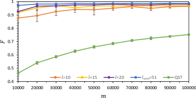
Figure 3: Performance of HLT on a 5-qubits Gibbs state created by a simulation of the VarQITE algorithm using Qiskit backend with a noise model. The plot shows the Fidelity between the exact simulated state and the HLT/QST-reconstructed state as a function of the total number of measurements ($m$). The number of SVs ($l$) used by HLT is shown in the legend. Measurements for QST were distributed equally over all $3^{5}$ different Pauli bases. Results are averaged over $10$ simulation runs, with error bars indicating one standard deviation.

In Fig. 3 we present the performance of HLT 5-qubits noisy numerical simulations. As in Fig. 1, we plot the fidelity of the HLT states with the actual state in the simulation. The plot shows HLT performance for different numbers of SVs and measurements $m$, and compares it with a traditional QST with the same number of measurements. HLT performed well even though the GH of the state was not entirely 2-local, because of the noise in the simulation. To be precise, the 3-local or more Pauli coefficients were $4.68\%$ of the GH norm (see Appendix E).

IV.1.3.   Quantum hardware results

In this subsection we present benchmarks of the HLT on actual quantum hardware. As in the previous section, we used the VarQITE algorithm to generate an approximate transverse Ising model Gibbs state on $N$ qubits by approximate imaginary time evolution to a maximally entangled state of $2N$ qubits.

Figure 4 presents the results of a $5$ qubits HLT on the ibmq_mumbai $27$-qubits backend . Unlike the numerical simulation case, here we did not know the exact quantum state. Therefore, in order to assess the quality of HLT state, we compared it to a high-precision QST state that was obtained using a much larger set of measurements: we used $2\times 10^{4}$ measurements on each of the $3^{5}$ QST bases, which amounts to almost $5$ millions measurements. In Appendix D and Table 2 we use numerical noisy simulations to estimate that for this number of qubits and measurements, the QST fidelity from the real quantum state is about $0.985$.

Figure 4a shows the fidelity of the QST state with the state reconstructed by HLT with merely $10^{4}$—$10^{5}$ measurements and $l=10,30$. Fidelity exceeded $0.98$ with $2\times 10^{4}$ measurements or more. We also used QST with diluted number of measurements, which achieved a fidelity of less than $0.7$ with the high-precision QST, using a total of $10^{5}$ measurements (Fig. 4a, yellow points). In order to further verify the above results, we extracted the four highest eigenvalues of HLT and QST reconstructed density matrices (Fig. 4b). Agreement of $0.01$ with the high-precision QST result was obtained with merely $25$ SVs, demonstrating the ability of HLT to predict global, non-linear properties of the state on quantum hardware.

a)

b)

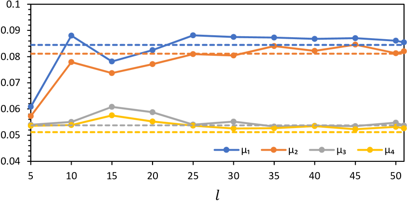
Figure 4: Quantum hardware results of HLT and QST using the ibmq_mumbai 27-qubits backend over $5$ qubits in a Gibbs state of the transverse-field Ising model. (a) The fidelity of HLT and QST as a function of the number of measurements $m$. The fidelity was calculated with respect to a high-precision QST, which used $2\times 10^{4}$ measurements in each of the $3^{5}$ QST bases (with estimated fidelity of above $0.985$). Subsets of the same measurements were used for QST and HLT in order to eliminate bias due to temporal fluctuations of device parameters. The plot shows a clear advantage of the HLT method, already with $l=10$ SVs. (b) The four highest eigenvalues, $\mu_{i}$, of HLT-reconstructed state with $10^{5}$ measurements as a function of $l$. Dashed lines show the four highest eigenvalues of the high-precision QST result.

Figure 5 shows the results of HLT on larger systems of $4-10$ qubits . Just as in the $5$ qubits case, we used the VarQITE algorithm to approximate the transverse model Ising Gibbs state on these systems. For $N>5$, QST of the entire system is not feasible because of the large number of measurements needed. Instead, to evaluate the HLT performance we used QST to reconstruct the states of all $3$-qubit contiguous subsystems (i.e $\left\{1,2,3\right\},\ldots,\left\{N-2,N-1,N\right\}$) and calculated the average fidelity between them and HLT-reconstructed states. The local QST was done using $8,192$ measurements in each of the QST $3^{3}$ bases, and as we argue in Appendix D, the expected QST fidelity in this case is above $0.995$. As shown in Fig. 5, average local fidelity results between the HLT and the local QST was above $0.99$ with $l=30$ and a modest number of $m=10^{5}$ measurements for any system size. For $N=10$ qubits, the low number of SVs used ($30$ out of $l_{max}=111$) was especially important for the optimization step, which would have taken days had we used the full $l_{max}$ SVs.

We end this subsection by noting that the actual Gibbs states prepared on the quantum hardware differed substantially from the ideal Transverse Ising model Gibbs state. This can be attributed to imperfections in the quantum hardware and the fact that the optimization of the variational algorithm was done on a classical simulation and not on the quantum hardware itself. As described in detail in Appendix E, the QST and HLT results show that the underlying Gibbs Hamiltonians were classical to some extent: their most dominant terms in the Pauli expansion were in the $Z$ basis. The HLT method is, of course, blind to this bias. The fact that it performed well on local Gibbs states that were different from the intended ones, demonstrates its capabilities to reconstruct unknown states with local GHs.

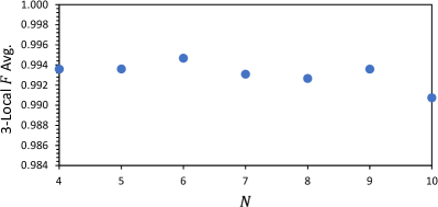
Figure 5: Quantum hardware results of HLT using the ibmq_toronto 27-qubits backend, for transverse-field Ising Gibbs states with $4$—$10$ qubits. The plot shows the average fidelity, over all $3$-qubits contiguous subsystems, between QST and HLT-reconstructed states as a function of the number of qubits $N$. QST was run separately on each subsystem, whereas using HLT with $10^{5}$ measurements and $30$ SVs the full state was reconstructed, from which the reduced density matrices of the subsystems were extracted. QST for each subsystem used $8,192$ measurements in each of the $3^{3}$ local bases (with an estimated fidelity above $0.995$).

IV.2.   GHZ state

A GHZ state [29], also called cat state, on $N$ qubits is defined as:

$$\frac{\left|0\right>^{\otimes N}+\left|1\right>^{\otimes N}}{\sqrt{2}}.$$

While the GHZ is not by itself a local Gibbs state, tracing out one or more qubits gives the reduced density matrix

$$\rho_{GHZ}=\frac{1}{2}\left(\left|0\ldots 0\rangle\langle 0\ldots 0\right|+\left|1\ldots 1\rangle\langle 1\ldots 1\right|\right).$$ (14)

This is the $T=0$ Gibbs state of the classical Ising Hamiltonian, and so by using

$$H_{GHZ}=-a\sum_{i=1}^{M-1}Z_{i}Z_{i+1}\quad,\quad a\gg 1.$$ (15)

we get

$$e^{-H_{GHZ}}=e^{aM}\bigg{[} \left|0\ldots 0\rangle\langle 0\ldots 0\right|+\left|1\ldots 1\rangle\langle 1\ldots 1\right|+$$

$$+\sum_{j=2}^{2^{M}-1}e^{-r_{j}a}\left|j\rangle\langle j\right|\bigg{]}\quad,\quad\forall j:\,\,r_{j}\geq 1,$$

which after normalization is a good approximation of $\rho_{GHZ}$ for large enough $a$.

We finally note that unlike the Gibbs state of the previous section, a GHZ state is an extremely “fragile” state, and even a small amount of noise can cause its reduced density matrix to drift away from a local Gibbs state. We see this effect in the following subsection, where we present quantum hardware HLT results of this state.

Quantum hardware results

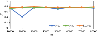
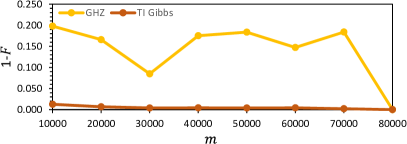
Figure 6: Quantum hardware results for the GHZ case. The plots show the HLT performance on the reduced density matrix of $5$ out of $6$ qubits in a GHZ state prepared on the $ibmq\_mumbai$ 27-qubits backend. Top: fidelity between the QST and the HLT reconstructed states. QST used $8,192$ measurements in each of the $3^{5}$ Pauli bases. HLT used between $10^{4}$ to $8\times 10^{4}$ measurements and different numbers of SVs as described in the legend. Bottom: convergence of infidelity for the GHZ states (yellow), with the transverse Ising Gibbs states shown as reference (brown). Points show infidelity between the HLT-reconstructed state with $8\times 10^{4}$ measurements and the HLT-reconstructed states using $m$ measurements, both with $l_{max}=51$ SVs.

Using the ibmq_mumbai 27-qubits backend we tested HLT on GHZ states on quantum hardware for a $5$-qubits reduced density matrix out of $6$ qubits . The GHZ state itself was created using a standard low-depth circuit that contained a Hadamard gate and 5 CNOT gates. Figure 6 (top) shows the fidelity between HLT-reconstructed states and a high-precision QST state as a function of the number of HLT measurements. The HLT states were calculated with $l=10,20,30$ SVs and $m$ varying from $10^{4}$ to $8\times 10^{4}$ measurements. The QST state was calculated using $8,192$ measurements on each of the $3^{5}$ different QST bases (a total of almost two million measurements). The same measurement results were used for both QST and HLT (with proper dilution) in order to eliminate bias due to temporal fluctuations of device parameters. Following Table 2 in Appendix D, we estimate the QST fidelity in this case to be more than $0.99$.

As clearly shown in the top panel of Fig. 6, the fidelity between the HLT state and the high-precision QST state is below $0.8$. This is in sharp contrast with the Gibbs state of the transverse Ising model Hamiltonian shown in Fig. 4a, where the HLT fidelity with $l=10,30$ quickly went above $0.95$.

As mentioned above, the relative failure of $k=2$ HLT can be attributed to the hardware noise, which, together with the fragility of the GHZ state, seems to introduce more $3$-local terms (or higher) to the Gibbs Hamiltonian. A possible solution could be increasing the locality of the Gibbs Hamiltonian in the method from $k=2$ to $k=3$ or $k=4$, which is however beyond the scope of the current work.

At this point, it is important to understand if it is possible to identify the failure of the $k=2$ HLT without relying on the high-precision QST results. Following the discussion in Sec. III.3, we compared the average local fidelity of HLT state with $l=l_{max}$ and $m=8\times 10^{4}$ with the local QST state. Also here, the fidelity never exceeded $0.91$, indicating a low global fidelity. Additionally, in Fig. 6 (bottom) we studied the convergence of HLT on GHZ states as a function of the number of measurements. The plot shows the infidelity of the HLT state with $m$ measurements and $l=l_{max}$ with the HLT state that was obtained with the maximal $m=8\times 10^{4}$ measurements and the same $l$. The figure (yellow line) clearly shows strong fluctuations in terms of $m$, which is yet another strong indication for the failure of the $k=2$ HLT. For comparison, we have plotted the same calculation for the previous case of the VarQITE generated Gibbs state (brown line). Unlike the Gibbs state, here a clear convergence is observed as soon as $m>2\times 10^{4}$.

V Discussion and Outlook

We suggest Hamiltonian Learning Tomography, a general tomography method for Gibbs state with local Hamiltonian, which uses moderate computational and quantum resources. It exploits Hamiltonian learning based on a constraint matrix for observables, to get a parametrized ansatz for the Gibbs Hamiltonian composed of the constraint matrix’s singular values. The ansatz is then optimized with respect to local measurement results, similar to EHT.

The use of the Hamiltonian learning algorithm to generate an ansatz removes the need for an a-priori knowledge of the Hamiltonian that parametrizes the state, as relied upon in EHT. We have shown in multiple examples that the ansatz requires a very low number of measurements, in comparison with common QST methods, for reaching a high tomography precision. Furthermore, using an optimization method circumvents the need for a gap in the constraint matrix and furthermore, the normalization of the state, which is enforced by the optimization method, provides the multiplicative factor of the Hamiltonian.

We implemented HLT and demonstrated it on states with a local GH, both in simulations and on IBM Quantum superconducting devices. At first, we verified HLT for $5$-qubit transverse-field Ising Gibbs state using high-precision QST. Then, the density matrix of states with $4$ to $10$ qubits on the quantum device were reconstructed with high fidelities, using a very low number of measurements in comparison with common QST methods. We have also provided two indicators for the performance of HLT that can be assessed from the experiment data. The first indicator is obtained by performing local QST for feasible sizes of qubit subsystems, and the second is the convergence of the HLT states. Both indicate that HLT did not perform well on the GHZ states created with the quantum device, due to a breaking of the locality of the Gibbs Hamiltonian.

Considering possible extensions of our results, we here focused on 1D Gibbs Hamiltonians with $k=2$ locality, but HLT can be easily implemented on systems with higher $k$ or spatial dimensions. We note that for the optimizations we ran, we have to be able to hold the entire $N$-qubits density matrix in the computer memory and manipulate it, making it suitable for intermediate sized systems of $2$—$14$ qubits. This is the main bottleneck of the method for scaling to a large number of qubits. An interesting direction for future research would be to lift this restriction, for example, either by some form of efficient exponentiation (i.e. low-order polynomial expansions for high-temperatures), or by using tensor networks [67], or both [68]. The efficiency of the presented tomography method in terms of the number of measurements, and the fact that it is easy to identify based on the experiment results states that fall outside of its scope, make it a useful tool for the verification of quantum states that are hard to characterize.

VI Acknowledgments

We thank Raz Firanko and Netanel Lindner for enlightening discussions. IA acknowledges the support of the Israel Science Foundation (ISF) under the Research Grants in Quantum Technologies and Science No. 2074/19, and the joint NRF-ISF Research Grant No. 3528/20.

Appendix A GH Reconstruction Error Estimation

In this appendix we derive the bound on the reconstruction error of the Gibbs Hamiltonian given in (9). This bound reveals how the reconstruction error decays with $l$ and therefore justifies using the lowest $l$ singular vectors of the CM in the ansatz.

Theorem 1.

Let $K$ be the exact constraint matrix of some Gibbs state $\rho$, and let $\tilde{K}=K+\epsilon E$ be the empirical constraint matrix, where $E$ is a random matrix with elements that are independent and identically distributed random normal variables and $\epsilon\ll 1$. Let $\bm{v}_{0}$ be the singular value of $K$ with the lowest singular value, and let $\tilde{\bm{c}}_{l}$ be the projection of $\bm{v}_{0}$ on the subspace of the first $l$ singular vectors of $\tilde{K}$. Finally, let $\lambda_{i}$ be the $i$’th singular value of $K$, sorted in ascending order. Then

$$\mathbb{E}\big{(}\left\|\tilde{\bm{c}}_{l}-\bm{v}_{0}\right\|^{2}\big{)}=\epsilon^{2}\sum_{i\geq l}\frac{1}{\lambda^{2}_{i}}+O(\epsilon^{3}),$$ (16)

where the averaging $\mathbb{E}(\cdot)$ is defined with respect to the underlying probability space in which $E$ is defined.

Proof.

To simplify the presentation, we move to Dirac notation and denote the right singular vectors of $K,\tilde{K}$ by $\{\left|v_{i}\right\rangle\},\{\left|\tilde{v}_{i}\right\rangle\}$ respectively. These should not be confused with the underlying quantum states. Now $\left|v_{0}\right\rangle$ is the lowest right singular vector of $K$ with a corresponding zero singular value that corresponds to the exact Gibbs Hamiltonian. Up to an overall factor, the GH that we reconstruct from $\tilde{K}$ using its lowest $l$ singular vectors corresponds to the projection of $\left|v_{0}\right\rangle$ on the subspace spanned by $\{\left|\tilde{v}_{i}\right\rangle\}_{i=1}^{l}$:

$$\left|\tilde{c}_{l}\right\rangle\stackrel{{\scriptstyle\mathrm{def}}}{{=}}\sum_{i=0}^{l-1}\left\langle\tilde{v}_{i}\right.\left|v_{0}\right\rangle\left|\tilde{v}_{i}\right\rangle.$$ (17)

Therefore, $\left|v_{0}\right\rangle-\left|\tilde{c}_{l}\right\rangle=\sum_{i\geq l}\left\langle\tilde{v}_{i}\right.\left|v_{0}\right\rangle\left|\tilde{v}_{i}\right\rangle$ and so

$$\left\|\left|v_{0}\right\rangle-\left|\tilde{c}_{l}\right\rangle\right\|^{2}=\sum_{i\geq l}|\left\langle\tilde{v}_{i}\right.\left|v_{0}\right\rangle|^{2}.$$ (18)

We estimate the above sum using first-order perturbation theory. By definition, $\tilde{K}=K+\epsilon E$, and therefore,

$$\tilde{K}^{T}\tilde{K} =(K+\epsilon E)^{T}(K+\epsilon E)$$

$$=K^{T}K+\epsilon(E^{T}K+K^{T}E)+\epsilon^{2}E^{T}E.$$ (19)

Treating $K^{T}K$ as an unperturbated Hamiltonian and $\epsilon(E^{T}K+K^{T}E+\epsilon E^{T}E)$ as a perturbation, we use first-order perturbation theory to estimate $\left\langle\tilde{v}_{i}\right.\left|v_{0}\right\rangle$. We note that if $(\left|v_{i}\right\rangle,\lambda_{i})$ are a pair of right singular-vector and singular value of $K$, then $(\left|v_{i}\right\rangle,\lambda_{i}^{2})$ are pair of eigenvector and eigenvalue of $K^{T}K$. This allows us to apply standard perturbation theory calculation [69] for $\left|\tilde{v}_{i}\right\rangle$:

$$\left|\tilde{v}_{i}\right\rangle=\left|v_{i}\right\rangle-\epsilon\sum_{j\neq i}\left|v_{j}\right\rangle\frac{\left\langle v_{j}\right|E^{T}K+K^{T}E\left|v_{i}\right\rangle}{\lambda_{j}^{2}-\lambda^{2}_{i}}+O(\epsilon^{2}).$$ (20)

Multiplying by $\left\langle v_{0}\right|$ and using the fact that $\lambda_{0}=0$, for any $i>0$ we get

$$\left\langle v_{0}\right.\left|\tilde{v}_{i}\right\rangle =\epsilon\frac{\left\langle v_{0}\right|E^{T}K+K^{T}E\left|v_{i}\right\rangle}{\lambda^{2}_{i}}+O(\epsilon^{2})$$

$$=\epsilon\frac{\left\langle v_{0}\right|E^{T}\left|u_{i}\right\rangle}{\lambda_{i}}+O(\epsilon^{2}),$$

where $\left|u_{i}\right\rangle$ is the $i$’th left singular vector of $K$ and we used $\left\langle v_{0}\right|K^{T}=0$ and $K\left|v_{i}\right\rangle=\lambda_{i}\left|u_{i}\right\rangle$. Plugging this back to Eq. (18), we get

$$\left\|\left|v_{0}\right\rangle-\left|\tilde{c}_{l}\right\rangle\right\|^{2}=\epsilon^{2}\sum_{i\geq l}\frac{|\left\langle v_{0}\right|E^{T}\left|u_{i}\right\rangle|^{2}}{\lambda^{2}_{i}}+O(\epsilon^{3}).$$

To proceed, we would like to take the average of the above equation with respect to the i.i.d random variables that define the entries of $E$. Expanding $\left|v_{0}\right\rangle,\left|u_{i}\right\rangle$ in the standard basis, we get

$$\mathbb{E} \big{(}|\left\langle v_{0}\right|E^{T}\left|u_{i}\right\rangle|^{2}\big{)}=\mathbb{E}\big{(}\left\langle v_{0}\right|E^{T}\left|u_{i}\right\rangle\left\langle u_{i}\right|E\left|v_{0}\right\rangle\big{)}$$

$$=\sum_{k,l,m,n}\left\langle v_{0}\right.\left|k\right\rangle\left\langle l\right.\left|u_{i}\right\rangle\left\langle u_{i}\right.\left|m\right\rangle\left\langle n\right.\left|v_{0}\right\rangle\mathbb{E}\big{(}E_{lk}E_{mn}\big{)}.$$

Then using the fact that the entries of $E$ are i.i.d. normal random variables, we conclude that $\mathbb{E}\big{(}E_{lk}E_{mn}\big{)}=\delta_{lm}\cdot\delta_{kn}$, and so

$$\mathbb{E}\big{(}|\left\langle v_{0}\right|E^{T}\left|u_{i}\right\rangle|^{2}\big{)} =\sum_{k,l}|\left\langle v_{0}\right.\left|k\right\rangle|^{2}\cdot|\left\langle l\right.\left|u_{i}\right\rangle|^{2}$$

$$=\left\|\left|v_{0}\right\rangle\right\|^{2}\cdot\left\|\left|u_{i}\right\rangle\right\|^{2}=1.$$

Overall then,

$$\mathbb{E}\big{(}\left\|\left|v_{0}\right\rangle-\left|\tilde{c}_{l}\right\rangle\right\|^{2}\big{)}=\epsilon^{2}\sum_{i\geq l}\frac{1}{\lambda^{2}_{i}}+O(\epsilon^{3}),$$

which proves the desired bound. ∎

Theorem 1 uses first-order perturbation theory to prove Eq. (16). Since to zero order the singular values of $K$ and $\tilde{K}$ coincide, $\lambda_{i}=\tilde{\lambda}_{i}+O(\epsilon)$, we can use the empirical data to estimate the reconstruction error as

$$\left\|\tilde{\bm{c}}_{l}-\bm{v}_{0}\right\|\simeq\epsilon\left(\sum_{i\geq l}\frac{1}{\tilde{\lambda}^{2}_{i}}\right)^{1/2}$$ (21)

where $\epsilon=O(\frac{1}{\sqrt{m}})$, and $m$ is the number of measurements used to estimate every entry of $\tilde{K}$. To verify the applicability of this approximation, we performed numerical simulations in which we calculated the LHS and the first-order RHS of Eq. (21), and plotted the histogram of their ratio for many random realizations. Specifically, for each pair of values $N\in\left\{5,6,7,8\right\},\epsilon\in\left\{10^{-2},10^{-3},10^{-4}\right\}$ we randomly picked ten normalized $2$-local Hamiltonians on $N$ qubits and computed their CM $K$. Then, we added to $K$ entries an i.i.d. Gaussian noise with amplitude $\epsilon$ to get $\tilde{K}$, and calculated the projection of $\bm{v}_{0}$ on the span of the lowest $l$ SVs of $\tilde{K}$, for a wide range of $l$ values, in order to find $\bm{\tilde{c}}_{l}$. The ratio between the LHS and the RHS of Eq. (21) was then calculated and averaged over all values of $N,\epsilon,l$. The results are shown on Fig. 7 with an average ratio between LHS and RHS of $0.993$, which fits Eq. (21).

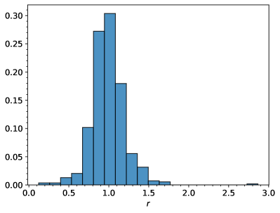
Figure 7: Histogram of the ratio between the reconstruction error for states with normalized random $2$-local GH and the error estimation from Eq. (21) $r=\left\|\tilde{\bm{c}}_{l}-\bm{v}_{0}\right\|/\left(\epsilon^{2}\sum_{i\geq l}\frac{1}{\tilde{\lambda}^{2}_{i}}\right)^{1/2}$. System size was $N=5-8$ qubits and a gaussian noise with amplitude $\epsilon\in\left\{10^{-2},10^{-3},10^{-4}\right\}$ was added to the CM to get $\tilde{K}$. Ten random normalized Hamiltonians were taken for each $N$ and $\epsilon$, and $r$ was calculated for a wide range of $l$ values. The average $r$ over $N,\epsilon,l$ was $0.993$.

Appendix B Gibbs State preparation with VarQITE

Imaginary time evolution can be used for Gibbs state preparation. Starting from maximally entangled state between sub-systems $A$ and $B$, we evolve the system under the Hamiltonian $H_{A}\otimes I_{B}$ for imaginary time $\beta/2$ and get the Gibbs state $e^{-\beta H}$ at sub-system $A$.

In Refs.[63, 70] a variational algorithm for imaginary time evolution, called VarQITE, is described. We followed the variational circuit architecture described in [70] and extended it from two qubits Gibbs state preparation up to 10-qubits, similar to Ref. [71] (ring topology with $R_{Y}$ rotations). We ran the variational imaginary time evolution for the transverse Ising model Hamiltonian (see Eq. (12)) using 10 iterations. We used an imaginary time $1/2$ to get a final state of $e^{-H}$. In order to avoid ill-conditioned linear equations during the algorithm, we used ridge regularization, as described in Ref. [70], with $\alpha=0.005$. The algorithm ran on the Qiskit simulator without noise. To assess the accuracy of the algorithm (on simulations), we calculated the exact Gibbs state using SciPy [61] matrix exponentiation, and compared it the output state of the noiseless variational circuit. The fidelity between these two states is given in Table 1. Fidelities above $0.96$ were obtained for up to $6$ qubits and above $0.9$ up to $10$ qubits.

The actual states prepared on the quantum hardware differed substantially from the intended Gibbs states (see Appendix E). Better results for preparing the Gibbs state on the quantum hardware could probably be obtained by performing the variational algorithm on the hardware, instead of simulation, which would also account for noise in the quantum hardware. However, running on quantum hardware would require a large amount of quantum resources. For Gibbs state on $N$ qubits, each algorithm iteration requires measuring $16N^{2}+4N$ different expectation values, each with different circuits. In addition, the above circuits include $2N+1$ qubits and up to twice the number of gates that are in the variational circuit. These long circuits would have a large noise accumulation which will affect the algorithm results. Moreover, if the optimization process takes too long, drifting errors in the underlying quantum hardware might hinder the quality of the final state. We leave this problem for future research.

# of qubits	Fidelity
2	0.9920
3	0.9865
4	0.9753
5	0.9663
6	0.9655
7	0.9491
8	0.9397
9	0.9395
10	0.9186

Table 1: Fidelity between exact 1D Ising model (Eq. (12)) Gibbs state and the final state of the variational Gibbs state preparation algorithm, without noise. 10 time iterations were made on simulation with a total (imaginary) time of $1/2$. The variational algorithm used ring architecture with parametrized $R_{Y}$ rotations before and after the ring (see Ref. [71] for details).

Appendix C Overlapping Local Tomography

As described in Sec. II.2, the expectation values that make up the entries of the constraint matrix are the commutators of $k$-local Paulis (Hamiltonians basis $\left\{S_{m}\right\}$) with $k+1$-local Paulis (constraints, $\left\{A_{q}\right\}$). Therefore, these are the expectation values of $2k$-local Paulis. In order to measure these expectation values efficiently, we used a cyclic basis measurements protocol called Overlapping Local Tomography, which is describe in Ref. [52]. In our case, the $1D$ chain is divided into cells of length $2k$, and each cell is measured using all $3^{2k}$ measurement basis configurations. The measurement bases are the same for each of the cells (see Fig. 8).

Ref. [52] also defines an extension of the protocol for $D$ dimensional lattices, which can be used to apply the HLT algorithm in higher dimensions.

Figure 8: Visual description of Overlapping local tomography measurement configurations for 1D chain with a unit length of $3$. Each consecutive $3$ qubits (different colors) form a unit cell which is measured in each of the $3^{3}$ basis configurations.

Appendix D Qiskit Quantum State Tomography

	Average Fidelity
	Gibbs		GHZ
	$m=8192$	$m=20000$	$m=8192$
N=2	0.9994	0.9998	0.9975
N=3	0.9965	0.9987	0.9957
N=4	0.9882	0.9937	0.9952
N=5	0.9742	0.9853	0.9949

Table 2: Average fidelity (over $10$ simulation runs) of Qiskit QST on variational Gibbs circuits for Transverse Ising (Eq. (12)) and GHZ states. QST reconstructed a state on $N$ qubits with $m$ measurements in each of the $3^{N}$ circuits.

This appendix summarizes the Qiskit QST algorithm, as described in Ref. [8]. Qiskit performs QST on $N$ qubits by measuring a state $\rho$ in all of the $3^{N}$ Pauli bases. Each basis measurement outcome can be represented as a projector $E_{i}$. Denoting $\vec{B}$ as the column vectorization of an operator $B$ (stacking $B$ columns into a single column) and $p_{i}$ as the measured probabilities for outcome $E_{i}$ gives the following linear equation:

$$E\vec{\rho}\stackrel{{\scriptstyle\mathrm{def}}}{{=}}\left(\begin{array}[]{c}\vec{E}_{1}^{\dagger}\vec{\rho}\\ \vdots\\ \vec{E}_{2\cdot 3^{N}}^{\dagger}\vec{\rho}\end{array}\right)=\left(\begin{array}[]{c}p_{1}\\ \vdots\\ p_{2\cdot 3^{N}}\end{array}\right)=\vec{p}.$$

This can be viewed as a least squares problem , whose solution is the pseudo-inverse $\vec{\rho}=\left(E^{T}E\right)^{-1}E^{T}\vec{p}$ . Due to finite statistics and quantum hardware noise, which affect $\vec{p}$, the above solution may be non-physical, i.e. $\rho$ might contain negative eigenvalues. Qiskit addresses this issue by using the algorithm described in Ref. [72] which computes the maximum-likelihood physical state for the results.

To assess the performance of Qiskit QST, which was used to verify the HLT results on quantum hardware, we ran it on numerical simulations. The simulations used the same variational circuits that created the Gibbs states in Sec. IV.1.2, and the same number of measurements used on the quantum devices, i.e., $3^{N}$ different bases with $8192$ or $20000$ measurements each. We ran each simulation for $10$ times and calculated the average fidelity between the QST state and the exact state of the simulation. Results are shown in Table 2. Evidently, for systems of up to $5$ qubits, the average fidelity was above $0.985$ with $20000$ measurements per basis. We also simulated Qiskit QST on GHZ states and obtained fidelities above $0.99$ for up to $5$ qubits.

These results suggest that we can trust the fidelity estimates of the HLT states with respect to the QST states on 5 qubits, as long as the fidelity is below 0.98. Higher fidelities might not necessarily represent the true fidelity of the HLT state with the underlying quantum state.

Appendix E Quantum Hardware State Preparation

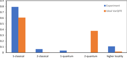
5Q Experiment		5Q Ideal VarQITE
IIIIZ	-1.919	IIIIZ	4.87185
IIZII	-1.525	ZIIII	4.85461
IZIII	-1.150	IIIZI	4.22767
IIIZI	-0.472	IZIII	4.14286
IYIII	-0.232	IIZII	4.13532
IIXII	-0.234	IXXII	4.11747
IIYII	-0.240	IIXXI	4.02958
IIIYI	-0.242	XXIII	3.75616
IXIII	-0.263	IIIXX	3.68091
IIIZZ	-0.736	IXZXI	0.92039

Figure 9: Pauli decomposition of Gibbs Hamiltonians. GHs extracted from the QST-reconstructed state with $2\times 10^{4}$ measurements in each of the $3^{5}$ bases shown at Fig. 4a (blue), versus the ideal VarQITE circuit outcome without noise (orange). Top: $\left\|H\right\|_{2}^{-2}\sum_{p_{i}}\left(\operatorname*{Tr}\left(Hp_{i}\right)\right)^{2}$ where the sum is over different normalized Paulis for each column: 1-classical are single site $Z$, 2-classical are $ZZ$ on nearest neighbours, 1-quantum are single site $X$ or $Y$, 2-quantum are $2$-local which are not 2-classical, and higher locality are all the rest. Bottom: ten coefficients with the largest absolute values in the full Pauli decomposition (any range) of the GHs.

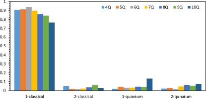
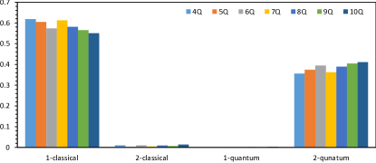
4Q		5Q		6Q		7Q
IIIZ	-1.389	IIIIZ	-1.869	IIIIIZ	-3.428	IIIZIII	-3.615
IIZI	-0.982	IIIZI	-1.696	IIZIII	-2.337	IIIIIIZ	-3.255
ZIII	-0.977	IZIII	-1.655	IIIZII	-2.300	IIIIZII	-3.031
IZII	-0.471	ZIIII	-1.535	ZIIIII	-1.621	IIIIIZI	-2.864
IIYZ	-0.141	IIZII	-1.521	IIIIZI	-1.083	IIZIIII	-2.469
XXII	-0.122	IIYII	-0.522	IZIIII	-0.911	IZIIIII	-2.445
ZZII	-0.149	IIIIY	-0.420	IIXIII	-0.353	ZIIIIII	-2.194
IZZI	-0.155	YZIII	-0.300	IIIIZZ	-0.397	IIIIIIY	-0.847
IYII	-0.224	IIZZI	-0.306	XIIIII	-0.453	IXXIIII	-0.702
IIZZ	-0.425	IZZII	-0.353	IIIIYI	-0.485	IIIIIZZ	-1.015

8Q		9Q		10Q
IIIIIIIZ	-4.487	IIIIIIIIZ	-5.918	IIIIIIIIIZ	-10.410
IIIIIZII	-4.450	IIIIIIZII	-5.581	IIIIIIIZII	-10.337
IIIZIIII	-4.014	IIIIZIIII	-5.113	IIIZIIIIII	0-8.202
IIIIZIII	-3.580	IIIIIZIII	-5.020	IIIIIZIIII	0-7.807
ZIIIIIII	-3.559	IIZIIIIII	-3.782	IIZIIIIIII	0-6.035
IIIIIIZI	-3.337	IIIZIIIII	-2.612	IIIIIIIIZI	0-5.465
IIZIIIII	-2.690	IZIIIIIII	-2.515	ZIIIIIIIII	0-5.308
IZIIIIII	-1.208	IIIIIIIZI	-2.095	IIIIIIIZZI	0-3.054
XIIIIIII	-1.279	ZIIIIIIII	-1.721	YIIIIIIIII	0-4.206
ZZIIIIII	-1.332	IIIIIIIZZ	-2.622	XIIIIIIIII	0-5.147

Figure 10: Pauli decomposition of Gibbs Hamiltonians. GHs extracted from HLT results shown at Fig. 5. Top: $\left\|H\right\|_{2}^{-2}\sum_{p_{i}}\left(\operatorname*{Tr}\left(Hp_{i}\right)\right)^{2}$ where the sum is over different normalized Paulis for each column: 1-classical are single site $Z$, 2-classical are $ZZ$ on nearest neighbours, 1-quantum are single site $X$ or $Y$, 2-quantum are $2$-local which are not 2-classical. HLT results with $k=2$ by definition does not have higher locality therefore it is not shown. Bottom: ten coefficients with the largest absolute values in the full Pauli decomposition (any range) of the GHs.

4Q		5Q		6Q		7Q
ZIII	-3.390	IIIIZ	4.87185	ZIIIII	6.915	IIIIIIZ	10.480
IIIZ	-3.115	ZIIII	4.85461	IIIIIZ	6.765	ZIIIIII	10.068
IIZI	-3.029	IIIZI	4.22767	IIZIII	6.277	IIZIIII	19.325
IXXI	-2.903	IZIII	4.14286	IIIIZI	6.163	IIIIIZI	19.139
IZII	-2.903	IIZII	4.13532	IIIXXI	6.039	IZIIIII	18.651
XXII	-2.687	IXXII	4.11747	IXXIII	5.844	IIIIZII	18.616
IIXX	-2.531	IIXXI	4.02958	IZIIII	5.795	IIIXXII	18.438
IXZX	-0.617	XXIII	3.75616	IIIZII	5.771	IIIZIII	18.205
XZXI	-0.607	IIIXX	3.68091	IIXXII	5.771	IIIIIXX	17.852
IIZZ	-0.526	IXZXI	0.92039	IIIIXX	5.393	XXIIIII	17.772

8Q		9Q		10Q
ZIIIIIII	14.527	ZIIIIIIII	19.000	IIIIIIIIIZ	27.529
IIIIIIIZ	13.417	IIIIIIIIZ	18.212	ZIIIIIIIII	26.464
IIIIIIZI	12.888	IIIIIIZII	18.182	IIIIIZIIII	25.502
IIIZIIII	12.319	IIIIZIIII	18.003	IIIZIIIIII	24.078
IIZIIIII	12.261	IZIIIIIII	17.756	IIIIZIIIII	24.029
XXIIIIII	12.061	IIIIIZIII	17.471	IIIXXIIIII	23.696
IIIXXIII	11.377	IIZIIIIII	17.432	IIIIIIZIII	23.303
IIIIIZII	11.368	IIIZIIIII	17.265	IIZIIIIIII	23.282
IZIIIIII	11.275	IIIIIXXII	17.163	IXXIIIIIII	22.232
IIIIXXII	11.014	IIIIXXIII	17.015	IIIIIIIIXX	22.227

Figure 11: Pauli decomposition of Gibbs Hamiltonians. GHs extracted from Ising Model VarQITE circuits’ ideal output — without hardware noise (see Appendix B, and specifically Table 1). Top: $\left\|H\right\|_{2}^{-2}\sum_{p_{i}}\left(\operatorname*{Tr}\left(Hp_{i}\right)\right)^{2}$ where the sum is over different normalized Paulis for each column: 1-classical are single site $Z$, 2-classical are $ZZ$ on nearest neighbours, 1-quantum are single site $X$ or $Y$, 2-quantum are $2$-local which are not 2-classical. Bottom: ten coefficients with the largest absolute values in the full Paulis decomposition (any range) of the GHs.

Noise within quantum hardware [73] causes imperfect state preparation. Therefore, the Gibbs states prepared by the algorithm from Appendix B were not exact.

We extracted the actual Gibbs Hamiltonians prepared by the quantum hardware using the density matrix from QST results and the matrix log function of SciPy [61]. We calculated the Pauli decomposition of these Hamiltonians using the trace inner product $\left<A,B\right>\stackrel{{\scriptstyle\mathrm{def}}}{{=}}\operatorname*{Tr}\left(A^{\dagger}B\right)$. The 10 coefficients with the largest absolute values in the decompositions of the results from Figs. 4a, 5 are shown at Figs. 9 (left),10 respectively, and can be compared to the values of the ideal VarQITE circuit, without hardware noise, in Figs. 9 (right),11 respectively. It is noted that the classical part of the Pauli decomposition (1-classical columns in Figs. 9, 10, 11) of the original Gibbs Hamiltonians was moderately changed by the noise on the quantum hardware. On the other hand, the $XX$ terms did not remain as in the original Hamiltonians, and their coefficients have changed drastically. Nevertheless, the prepared Gibbs state was not entirely classical, as it still contained non-negligible non-commuting terms. Furthermore, the Gibbs Hamiltonians remained almost $2$-local (as the original Gibbs Hamiltonians), which explains the success of the HLT method.

GHZ states were also subject to noise during their preparations. However, in this case, the noise led to highly non-local Gibbs Hamiltonians, which is reflected in the non-locality of their Pauli decomposition. Indeed, in the case of 5 qubits (obtained after preparing a 6-qubit GHZ state and tracing over one qubit), the resultant Gibbs Hamiltonian had a lot of weight on 3-local and higher terms. Summing over all the contributions of the 2-local, nearest-neighbor Pauli operators, we obtained

$$\left\|H\right\|_{2}^{-2}\sum_{\text{2-local $P_{s}$}}\left(\operatorname*{Tr}\left(HP_{s}\right)\right)^{2}<0.6.$$

In other words, over $40\%$ of the weight of the Gibbs Hamiltonian was in non-local terms.

References

- Vogel and Risken [1989] K. Vogel and H. Risken, Phys. Rev. A 40, 2847 (1989).
- White et al. [1999] A. G. White, D. F. V. James, P. H. Eberhard, and P. G. Kwiat, Physical Review Letters 83, 3103 (1999).
- Leonhardt [1995] U. Leonhardt, Physical Review Letters 74, 4101 (1995).
- Wang et al. [2016] X.-L. Wang, L.-K. Chen, W. Li, H.-L. Huang, C. Liu, C. Chen, Y.-H. Luo, Z.-E. Su, D. Wu, Z.-D. Li, H. Lu, Y. Hu, X. Jiang, C.-Z. Peng, L. Li, N.-L. Liu, Y.-A. Chen, C.-Y. Lu, and J.-W. Pan, Physical Review Letters 117, 10.1103/physrevlett.117.210502 (2016).
- Thew et al. [2002] R. T. Thew, K. Nemoto, A. G. White, and W. J. Munro, Physical Review A 66, 10.1103/physreva.66.012303 (2002).
- Lee [2002] J.-S. Lee, Physics Letters A 305, 349 (2002).
- Resch et al. [2005] K. J. Resch, P. Walther, and A. Zeilinger, Physical Review Letters 94, 10.1103/physrevlett.94.070402 (2005).
- Qis [2021] Qiskit: Quantum tomography (2021).
- Paris and Řeháček [2004] M. Paris and J. Řeháček, eds., Quantum State Estimation (Springer Berlin Heidelberg, 2004).
- Haah et al. [2017] J. Haah, A. W. Harrow, Z. Ji, X. Wu, and N. Yu, IEEE Transactions on Information Theory 63, 5628 (2017).
- Torlai et al. [2018] G. Torlai, G. Mazzola, J. Carrasquilla, M. Troyer, R. Melko, and G. Carleo, Nature Physics 14, 447 (2018).
- Gross et al. [2010] D. Gross, Y.-K. Liu, S. T. Flammia, S. Becker, and J. Eisert, Physical Review Letters 105, 10.1103/physrevlett.105.150401 (2010).
- Häffner et al. [2005] H. Häffner, W. Hänsel, C. F. Roos, J. Benhelm, D. C. al kar, M. Chwalla, T. Körber, U. D. Rapol, M. Riebe, P. O. Schmidt, C. Becher, O. Gühne, W. Dür, and R. Blatt, Nature 438, 643 (2005).
- Titchener et al. [2018] J. G. Titchener, M. Gräfe, R. Heilmann, A. S. Solntsev, A. Szameit, and A. A. Sukhorukov, npj Quantum Information 4, 10.1038/s41534-018-0063-5 (2018).
- Cramer et al. [2010] M. Cramer, M. B. Plenio, S. T. Flammia, R. Somma, D. Gross, S. D. Bartlett, O. Landon-Cardinal, D. Poulin, and Y.-K. Liu, Nature communications 1, 1 (2010).
- Aaronson [2018] S. Aaronson, Shadow tomography of quantum states (2018), arXiv:1711.01053 [quant-ph] .
- Huang et al. [2020] H.-Y. Huang, R. Kueng, and J. Preskill, Nature Physics 16, 1050 (2020).
- Rambach et al. [2021] M. Rambach, M. Qaryan, M. Kewming, C. Ferrie, A. G. White, and J. Romero, Physical Review Letters 126, 100402 (2021).
- von Neumann [2018] J. von Neumann, Mathematical Foundations of Quantum Mechanics: New Edition, edited by N. A. Wheeler (Princeton University Press, 2018).
- Reichental et al. [2018] I. Reichental, A. Klempner, Y. Kafri, and D. Podolsky, Phys. Rev. B 97, 134301 (2018).
- Srednicki [1994] M. Srednicki, Phys. Rev. E 50, 888 (1994).
- Deutsch [2018] J. M. Deutsch, Reports on Progress in Physics 81, 082001 (2018).
- Amin et al. [2018] M. H. Amin, E. Andriyash, J. Rolfe, B. Kulchytskyy, and R. Melko, Physical Review X 8, 10.1103/physrevx.8.021050 (2018).
- Somma et al. [2008] R. D. Somma, S. Boixo, H. Barnum, and E. Knill, Physical Review Letters 101, 10.1103/physrevlett.101.130504 (2008).
- Brandao and Svore [2017] F. G. S. L. Brandao and K. Svore, Quantum speed-ups for semidefinite programming (2017), arXiv:1609.05537 [quant-ph] .
- Bairey et al. [2019] E. Bairey, I. Arad, and N. H. Lindner, Physical Review Letters 122, 10.1103/physrevlett.122.020504 (2019).
- Kokail et al. [2021a] C. Kokail, R. van Bijnen, A. Elben, B. Vermersch, and P. Zoller, Nature Physics 17, 936–942 (2021a).
- IBM [2021] IBM Quantum (2021).
- Greenberger et al. [1989] D. M. Greenberger, M. A. Horne, and A. Zeilinger, in Bell’s Theorem, Quantum Theory and Conceptions of the Universe (Springer Netherlands, 1989) pp. 69–72.
- Lifshitz [2022] Y. Y. Lifshitz, Hamiltonian learning tomography - github (2022).
- Dalmonte et al. [2018] M. Dalmonte, B. Vermersch, and P. Zoller, Nature Physics 14, 827 (2018).
- Kokail et al. [2021b] C. Kokail, B. Sundar, T. V. Zache, A. Elben, B. Vermersch, M. Dalmonte, R. van Bijnen, and P. Zoller, arXiv preprint arXiv:2105.04317 (2021b).
- Calabrese and Cardy [2009] P. Calabrese and J. Cardy, Journal of Physics A: Mathematical and Theoretical 42, 504005 (2009).
- Bisognano and Wichmann [1975] J. J. Bisognano and E. H. Wichmann, Journal of Mathematical Physics 16, 985 (1975).
- Bisognano [1976] J. J. Bisognano, Journal of Mathematical Physics 17, 303 (1976).
- Giudici et al. [2018] G. Giudici, T. Mendes-Santos, P. Calabrese, and M. Dalmonte, Physical Review B 98, 10.1103/PhysRevB.98.134403 (2018).
- Granade et al. [2012] C. E. Granade, C. Ferrie, N. Wiebe, and D. G. Cory, New Journal of Physics 14, 103013 (2012).
- Wiebe et al. [2014a] N. Wiebe, C. Granade, C. Ferrie, and D. Cory, Physical Review A 89, 10.1103/physreva.89.042314 (2014a).
- Wiebe et al. [2014b] N. Wiebe, C. Granade, C. Ferrie, and D. Cory, Physical Review Letters 112, 10.1103/physrevlett.112.190501 (2014b).
- Wang et al. [2017] J. Wang, S. Paesani, R. Santagati, S. Knauer, A. A. Gentile, N. Wiebe, M. Petruzzella, J. L. O’Brien, J. G. Rarity, A. Laing, and M. G. Thompson, Nature Physics 13, 551 (2017).
- da Silva et al. [2011] M. P. da Silva, O. Landon-Cardinal, and D. Poulin, Physical Review Letters 107, 210404 (2011).
- Li et al. [2020] Z. Li, L. Zou, and T. H. Hsieh, Physical review letters 124, 160502 (2020).
- Wang et al. [2015] S.-T. Wang, D.-L. Deng, and L.-M. Duan, New Journal of Physics 17, 093017 (2015).
- Zhang and Sarovar [2014] J. Zhang and M. Sarovar, Physical review letters 113, 080401 (2014).
- Samach et al. [2021] G. O. Samach, A. Greene, J. Borregaard, M. Christandl, D. K. Kim, C. M. McNally, A. Melville, B. M. Niedzielski, Y. Sung, D. Rosenberg, M. E. Schwartz, J. L. Yoder, T. P. Orlando, J. I.-J. Wang, S. Gustavsson, M. Kjaergaard, and W. D. Oliver, Lindblad tomography of a superconducting quantum processor (2021), arXiv:2105.02338 [quant-ph] .
- Haah et al. [2021] J. Haah, R. Kothari, and E. Tang, arXiv preprint arXiv:2108.04842 (2021).
- Anshu et al. [2021] A. Anshu, S. Arunachalam, T. Kuwahara, and M. Soleimanifar, Nature Physics , 1 (2021).
- Rudinger and Joynt [2015] K. Rudinger and R. Joynt, Physical Review A 92, 10.1103/physreva.92.052322 (2015).
- Kieferová and Wiebe [2017] M. Kieferová and N. Wiebe, Physical Review A 96, 062327 (2017).
- Kappen [2020] H. J. Kappen, Journal of Physics A: Mathematical and Theoretical 53, 214001 (2020).
- Evans et al. [2019] T. J. Evans, R. Harper, and S. T. Flammia, arXiv preprint arXiv:1912.07636 (2019).
- Zubida et al. [2021] A. Zubida, E. Yitzhaki, N. H. Lindner, and E. Bairey, Optimized hamiltonian learning from short-time measurements (2021), arXiv:2108.08824 [quant-ph] .
- Bubeck [2014] S. Bubeck, arXiv preprint arXiv:1405.4980 (2014).
- Bellman [1957] R. Bellman, Press Princeton, New Jersey (1957).
- Van Der Maaten et al. [2009] L. Van Der Maaten, E. Postma, J. Van den Herik, et al., J Mach Learn Res 10, 13 (2009).
- Branch et al. [1999] M. A. Branch, T. F. Coleman, and Y. Li, SIAM Journal on Scientific Computing 21, 1 (1999).
- Anshu et al. [2020] A. Anshu, S. Arunachalam, T. Kuwahara, and M. Soleimanifar, in 2020 IEEE 61st Annual Symposium on Foundations of Computer Science (FOCS) (IEEE, 2020) pp. 685–691.
- Qiskit Contributors [2021] Qiskit Contributors, Qiskit: An open-source framework for quantum computing (2021).
- Uhlmann [1976] A. Uhlmann, Reports on Mathematical Physics 9, 273 (1976).
- Jozsa [1994] R. Jozsa, Journal of Modern Optics 41, 2315 (1994).
- SciPy 1.0 Contributors [2020] SciPy 1.0 Contributors, Nature Methods 17, 261 (2020).
- Paszke et al. [2019] A. Paszke, S. Gross, et al., in Advances in Neural Information Processing Systems 32, edited by H. Wallach, H. Larochelle, A. Beygelzimer, F. d’Alché Buc, E. Fox, and R. Garnett (Curran Associates, Inc., 2019) pp. 8024–8035.
- Yuan et al. [2019] X. Yuan, S. Endo, Q. Zhao, Y. Li, and S. C. Benjamin, Quantum 3, 191 (2019).
- Note [1] The experiment was conducted on the device ibmq_mumbai on 23/11/2021. Backends are listed in https://quantum-computing.ibm.com/.
- Note [2] The experiment was conducted on the device ibmq_toronto on 06/11/2021.
- Note [3] The experiment was conducted on the device ibmq_mumbai on 26/08/2021.
- Torlai et al. [2020] G. Torlai, C. J. Wood, A. Acharya, G. Carleo, J. Carrasquilla, and L. Aolita, arXiv preprint arXiv:2006.02424 (2020).
- Vanhecke et al. [2021] B. Vanhecke, D. Devoogdt, F. Verstraete, and L. Vanderstraeten, arXiv preprint arXiv:2112.01507 (2021).
- Schrödinger [1926] E. Schrödinger, Ann. Phys.(Berl.) 385, 437 (1926).
- Zoufal et al. [2021] C. Zoufal, A. Lucchi, and S. Woerner, Quantum Machine Intelligence 3, 10.1007/s42484-020-00033-7 (2021).
- Lehtonen [2021] L. Lehtonen, Analysis and implementation of quantum Boltzmann machines, Master’s thesis, Helsingin yliopisto (2021).
- Smolin et al. [2012] J. A. Smolin, J. M. Gambetta, and G. Smith, Physical review letters 108, 070502 (2012).
- Clerk et al. [2010] A. A. Clerk, M. H. Devoret, S. M. Girvin, F. Marquardt, and R. J. Schoelkopf, Reviews of Modern Physics 82, 1155 (2010).