Symbolic Specialization of Rewriting Logic Theories with Presto 

Abstract

This paper introduces Presto, a symbolic partial evaluator for Maude’s rewriting logic theories that can improve system analysis and verification. In Presto, the automated optimization of a conditional rewrite theory $\mathcal{R}$ (whose rules define the concurrent transitions of a system) is achieved by partially evaluating, with respect to the rules of $\mathcal{R}$, an underlying, companion equational logic theory $\mathcal{E}$ that specifies the algebraic structure of the system states of $\mathcal{R}$. This can be particularly useful for specializing an overly general equational theory $\mathcal{E}$ whose operators may obey complex combinations of associativity, commutativity, and/or identity axioms, when being plugged into a host rewrite theory $\mathcal{R}$ as happens, for instance, in protocol analysis, where sophisticated equational theories for cryptography are used. Presto  implements different unfolding operators that are based on folding variant narrowing (the symbolic engine of Maude’s equational theories). When combined with an appropriate abstraction algorithm, they allow the specialization to be adapted to the theory termination behavior and bring significant improvement while ensuring strong correctness and termination of the specialization. We demonstrate the effectiveness of Presto in several examples of protocol analysis where it achieves a significant speed-up. Actually, the transformation provided by Presto may cut down an infinite folding variant narrowing space to a finite one, and moreover, some of the costly algebraic axioms and rule conditions may be eliminated as well. As far as we know, this is the first partial evaluator for Maude that respects the semantics of functional, logic, concurrent, and object-oriented computations. Under consideration in Theory and Practice of Logic Programming (TPLP).

1 Introduction

Partial evaluation (PE) is a general and powerful optimization technique that automatically specializes a program to a part of its input that is known statically [Jones et al., 1993]. PE is motivated by the fact that dedicated programs tend to operate more efficiently than general-purpose ones. It has found applications ranging from compiler optimization to test case generation, among many others [Cadar and Sen, 2013, Cook and Lämmel, 2011]. In the context of logic programming (LP), partial evaluation is often called partial deduction (PD), while the term partial evaluation is often reserved for the specialization of impure logic programs. PD not only allows input variables to be instantiated with constant values but it also deals with terms that may contain logic variables, thus providing extra capabilities for program specialization [Martens and Gallagher, 1995].

Rewriting Logic (RWL) is a very general logical and semantic framework that is particularly suitable for modeling and analyzing complex, highly nondeterministic software systems [Martí-Oliet and Meseguer, 2002]. Rewriting Logic is efficiently implemented in the high-performance language Maude [Clavel et al., 2007], which seamlessly integrates functional, logic, concurrent, and object-oriented computations. A Maude rewrite theory $\mathcal{R}=(\Sigma,E\uplus B,R)$ combines a term rewriting system $R$, which specifies the concurrent transitions of a system (for a signature $\Sigma$ of program operators together with their type definition), with an equational theory $\mathcal{E}=(\Sigma,E\uplus B)$ that specifies system states as terms of an algebraic datatype. The equational theory $\mathcal{E}$ contains a set $E$ of equations and a set $B$ of axioms (i.e., distinguished equations that specify algebraic laws such as commutativity, associativity, and unity for some theory operators that are defined on $\Sigma$). The equations of $E$ are implicitly oriented from left to right as rewrite rules and operationally used as simplification rules, while the axioms of $B$ are mainly used for $B$-matching so that rewrite steps in $\mathcal{R}$ are performed modulo the equations and axioms of $E\uplus B$.

For instance, in protocol specification, the equations of $E$ are often used to define the cryptoarithmetic functions that are used in the protocol transition rules (e.g., addition, exponentiation, and exclusive-or), while the axioms of $B$ specify properties of the cryptographic primitives (e.g., commutativity of addition and multiplication). For example, consider the (partial) specification of integer numbers defined by the equations $E=\{X+0=X,~{}X+s(Y)=s(X+Y),~{}p(s(X))=X,~{}s(p(X))=X\}$, where variables $X$, $Y$ are of sort Int (types are called sorts in RWL), operators $p$ and $s$ respectively stand for the predecessor and successor functions, and $B$ contains the commutativity axiom $X+Y=Y+X$. Also consider that the program signature $\Sigma$ contains a binary state constructor operator $\langle\_,\_\rangle:$ Int x Int $\rightarrow$ State for a new sort State that models a simple network of processes that consume a token from one place (denoted by the first component of the state) and transmit it to another place (the second component), keeping the total amount of tokens invariant. The system state $t=\langle s(0),s(0)+p(0)\rangle$ can be rewritten to $\langle 0,s(0)\rangle$ (modulo the equations of $E$ and the commutativity of $+$) using the following rule that specifies the system dynamics:

$$\langle A,B\rangle\Rightarrow\langle p(A),s(B)\rangle,\mbox{ where }A\mbox{ and }B\mbox{ are variables of sort {\tt Int}}$$ (1)

Multiparadigm, functional logic languages combine features from functional programming (efficient evaluation strategies, nested expressions, genericity, advanced typing, algebraic data types) and logic programming (logical variables, partial data structures, nondeterministic search for solutions, constraint solving modulo theories) [Meseguer, 1992b, Hanus, 1997, Escobar, 2014]. The operational principle that supports functional and logic language integration is called narrowing [Fay, 1979, Slagle, 1974], which is a goal-solving mechanism that subsumes the resolution principle of logic languages and the reduction principle of functional languages. Roughly speaking, narrowing can be seen as a generalization of term rewriting that allows free variables in terms (as in logic programming) and that non-deterministically reduces these partially instantiated function calls by using unification (instead of pattern-matching) at each reduction step [Hanus, 1994].

Besides rewriting with rules modulo equations and axioms, Maude provides full native support for narrowing computations in rewrite theories since Maude version 3.0 (2020). This endows Maude with symbolic reasoning capabilities (e.g., symbolic reachability analysis in rewrite theories based on narrowing) and unification modulo user-definable equational theories. In our example theory, a narrowing reachability goal from $\langle V+V,0+V\rangle$ to $\langle p(0),s(0)\rangle$ succeeds (in one step) with computed substitution $\{V\mapsto 0\}$, which might signal a possible programming error in rule (1) since the number of available tokens in the first component of the state becomes negative, thereby pinpointing a token shortage. This kind of advanced, LP-like reasoning capability based on narrowing goes beyond standard, rewrite-based equational reasoning that does not support symbolic reachability analysis because input variables are simply handled as constants. Symbolic reasoning methods that are based on narrowing and their applications are generally discussed in [Meseguer, 2020, Meseguer, 2021]. For a very brief account of Maude’s rewriting and narrowing principles, we refer to [Alpuente et al., 2019b].

In this paper, we develop the narrowing-based partial evaluator Presto  and show how it can have a tremendous impact on the symbolic analysis of concurrent systems that are modeled as Maude rewrite theories. Traditional partial evaluation techniques typically remove some computation states by performing as much program computation as possible, hence contracting the search space because some transitions are eliminated. However, in the specialization of concurrent systems that are specified by Maude rewrite theories, we are only interested in compressing the deterministic, functional computations (which normalize the system states and are encoded by means of the theory equations) while preserving all concurrent state transitions (which are defined by means of the rewrite rules). This ensures that all reachable system states are preserved so that any reachability property of the original concurrent system can be correctly analyzed in the specialized one.

Given a rewrite theory $\mathcal{R}=(\Sigma,E\uplus B,R)$ our method proceeds by partially evaluating the underlying equational theory $\mathcal{E}=(\Sigma,E\uplus B)$ with respect to the function calls in the rules of $\mathcal{R}$ in such a way that $\mathcal{E}$ gets rid of any possible overgenerality. By doing this, only the functional computations in $\mathcal{E}$ are compressed by partial evaluation, while keeping every system state in the search space of the concurrent computations of $\mathcal{R}$. Partial evaluation can dramatically help in this process by introducing polyvariance (i.e., specializing a given function into different variants according to distinct invocation contexts [Martens and Gallagher, 1995]). The transformation performed by Presto is non-trivial because, depending on the properties of both theories ($\mathcal{E}$ and $\mathcal{R}$), the right unfolding and abstraction operators are needed to efficiently achieve the largest optimization possible while ensuring termination and total correctness of the transformation.

The partial evaluator Presto  provides near-perfect support for the Maude language; specifically, it deals with all of the features that are currently supported by Maude’s narrowing infrastructure. This effort is remarkable for at least two reasons: (i) Maude has quite sophisticated features (subtype polymorphism, pattern matching and equational unification modulo associativity, commutativity and identity axioms, equations, rules, modules, objects, etc.); and (ii) in order to efficiently achieve aggressive specialization that scales to real-world problems, the key components of the Presto system needed to be thoroughly investigated and highly optimized over the years. This is because equational problems such as order-sorted equational homeomorphic embedding and order-sorted equational least general generalization are much more costly than their corresponding “syntactic” counterparts and achieving proper formalizations and efficient implementations has required years [Alpuente et al., 2008, Alpuente et al., 2009b, Alpuente et al., 2014b, Alpuente et al., 2019a, Alpuente et al., 2020b, Alpuente et al., 2020c, Alpuente et al., 2021b].

1.1 Related work

Traditional applications of partial evaluation include the optimization of programs that explore a state space by trying to reduce the amount of search. Relevant prior work includes the use of partial deduction to optimize a theorem prover with respect to a given theory [de Waal and Gallagher, 1994] and to refine infinite state model checking [Leuschel and Gruner, 2001], where both the theorem prover and the model checker are written as a logic program that searches for a proof, and the experiments use a standard partial evaluator that is supplemented with abstract interpretation [Cousot and Cousot, 1977] so that infinite branches in the search space are removed. Also, the specialization of concurrent processes that are modeled by (infinite state) Petri nets or by means of process algebras is performed in [Leuschel and Lehmann, 2000] by a combination of partial deduction and abstract interpretation.

Among the vast literature on program specialization, the partial evaluation of functional logic programs [Alpuente et al., 1998b, Albert et al., 2002, Hanus and Peemöller, 2014] is the closest to our work. The narrowing-driven Partial Evaluation (NPE) algorithm of [Alpuente et al., 1998b], implemented in the Indy system [Albert et al., 1998], extends to narrowing the classical PD scheme of [Martens and Gallagher, 1995] and was proved to be strictly more powerful than the PE of both logic programs and functional programs [Alpuente et al., 1998b], with a potential for specialization that is comparable to conjunctive partial deduction (CPD) and positive supercompilation [De Schreye et al., 1999]. Early instances of this framework implemented partial evaluation algorithms for different narrowing strategies, including lazy narrowing [Alpuente et al., 1997], innermost narrowing [Alpuente et al., 1998b], and needed narrowing [Albert et al., 1999, Alpuente et al., 2005].

NPE was extended in [Alpuente et al., 2020b] to the specialization of order-sorted equational theories and implemented in the partial evaluator for equational theories Victoria. This was essentially achieved by generalizing the key NPE ingredients to work with order-sorted equations and axioms: 1) a tree unfolding operator based on folding variant narrowing that ensures strong correctness of the transformation; 2) a novel notion of order-sorted equational homeomorphic embedding that achieves local termination (i.e., finiteness of unfolding); 3) a suitable notion of order-sorted equational closedness (coveredness of the tree leaves modulo axioms) that ensures strong completeness; and 4) an abstraction operator based on order-sorted equational least general generalization that provides global termination of the whole specialization process. However, the partial evaluator Victoria is only able to specialize deterministic and terminating equational theories, while the Presto system described in this article deals with non-deterministic and non-terminating rewrite theories that allow concurrent systems to be modeled and model-checked. For a detailed discussion of the literature related to narrowing-driven partial evaluation, we refer to [Alpuente et al., 2020b].

The partial evaluator Presto  implements our most ambitious generic specialization framework for RWL. Currently, there is hardly any system that can automatically optimize rich rewrite theories that include sorts, subsort overloading, rules, equations, and algebraic axioms. Actually, there are very few transformations in the related literature that can improve the analysis of Maude’s rewrite theories and they are only known to the skilled practitioner, and, moreover, they lack automated tool support. For instance, the total evaluation of [Meseguer, 2020], which only applies to a restricted class of equational theories called constructor finite variant theories. Moreover, unlike the optimization that is achieved by Presto,  none of the existing transformations respects the narrowing semantics of the theory (both values and computed substitutions), just its ground value semantics or its reduction (normal form) semantics [Alpuente et al., 2010, Lucas and Meseguer, 2016].

Many kinds of tools are built in Maude that rely on reflection and theory transformations and preserve specific properties such as invariants or termination behavior. Full-Maude [Clavel et al., 2020], Real-time Maude [Ölveczky and Meseguer, 2008], MTT [Durán et al., 2008], and Maude-NPA [Escobar et al., 2009] are prominent examples. Equational abstraction [Meseguer et al., 2008, Bae et al., 2013] reduces an infinite state system to a finite quotient of the original system algebra by introducing some extra equations that preserve certain temporal logic properties. Explicit coherence (a kind of confluence between rules, equations, and axioms) is necessary for executability purposes and also relies on rewrite theory transformations [Viry, 2002, Meseguer, 2020, Durán et al., 2020b]. Also the semantic $\mathbb{K}$-framework [Roşu, 2017], the model transformations of [Rodríguez et al., 2019], and the automated program correction technique of [Alpuente et al., 2019c, Alpuente et al., 2020a] are based on sophisticated program transformations that preserve the reduction semantics of the original theory. Nevertheless, none of them aim to achieve program optimization.

The generic narrowing-driven partial evaluation scheme was originally formulated in [Alpuente et al., 2022] for (unconditional) rewrite theories. An instance of the framework that mimicks the total evaluation of [Meseguer, 2020] can be found in [Alpuente et al., 2021a]. Experiments with a preliminary version of the Presto system together with its basic underpinnings can also be found in [Alpuente et al., 2022].

1.2 Contributions

The original contributions of this article with respect to the partial evaluation scheme for unconditional rewrite theories presented in [Alpuente et al., 2022] are as follows.

1. We extend the generic narrowing-driven partial evaluation scheme of [Alpuente et al., 2022] to the specialization of rewrite theories that may contain conditional rules. Given the rewrite theory $\mathcal{R}=(\Sigma,E\uplus B,R)$, this is done as follows. First, the equational theory is partially evaluated with respect to both the function calls in the right-hand sides and the conditions of the rewrite rules of $R$. Then, a post-processing refactoring transformation is applied to both equations and rules that gets rid of unnecessary symbols and delivers a more efficient, computationally equivalent rewrite theory where some of the costly algebraic axioms and rule conditions may simply get removed. The new rule condition simplification algorithm is quite inexpensive and does not modify the program semantics.

2. A novel transformation called topmost extension is provided that achieves in one shot the two executability conditions that are required for the completeness of narrowing in Maude rewrite theories: the explicit coherence of rules with respect to equations and axioms, and the topmost requirement on rules that forces all rewrites to happen on the whole state term —not on its subterms. We demonstrate that the topmost transformation is correct and preserves the solutions of the original theory so narrowing-based symbolic reachability analysis is enabled for all rewrite theories after the topmost transformation.

3. We apply our novel results on the topmost extension to support narrowing-based specialization for object-oriented specifications. It is worth noting that Maude’s object-oriented rules are typically non-topmost and they were not covered by [Alpuente et al., 2022].

4. We have expanded the Presto system that implements the partial evaluation scheme of [Alpuente et al., 2022] both to cope with conditions in rules and to handle Maude object-oriented modules that (in addition to equations, axioms, and rewrite rules) support classes, objects, messages, multiple class inheritance, and object interaction rules.

5. We also endowed Presto with an automated checker for: 1) strong irreducibility, a mild condition enforcing that the left-hand sides of the rewrite rules of $R$ cannot be narrowed in $E$ modulo $B$, which is needed for the strong completeness of our specialization method [Alpuente et al., 2020b]; and 2) a novel property called U-tolerance ensuring that least general generalization with identity axioms is finitary even if function symbols have more than one unit element [Alpuente et al., 2021b]. This scenario can occur when a rewrite theory contains multiple overloaded function symbols associated with distinct identity elements. Although most commonly occurring theories satisfy these properties, these checks are an important addition to the system because checking them manually is painful, since they involve term unification modulo any combination of equational axioms, which is difficult to calculate by hand.

6. We describe the system capabilities and provide an empirical evaluation of Presto on a set of protocol analysis problems where it demonstrates a significant speed-up.

1.3 Plan of the paper

In Section 2, we provide some preliminary notions on RWL, and we introduce a leading example that will be used throughout the paper to describe the specialization capabilities of Presto. Section 3 recalls the narrowing-based symbolic principles of Maude and formalizes an automatic program transformation that generates topmost rewrite theories for which the narrowing machinery for solving symbolic reachability problems can be effectively used. Specifically it enables symbolic reachability for object-oriented rewrite theories. In Section 4, we present our basic specialization scheme for conditional rewrite theories and describe its core functionality. Section 5 provides two instantiations of the specialization scheme that exploit two distinct unfolding operators that are suitable for theories that respectively have either an infinite behavior or a finite behavior with regard to narrowing computations. In Section 6, we present an overview of Presto’s main implementation choices and some additional tool features that allow the user to inspect the intermediate results of the specialization as well as to visualize all of the narrowing trees that are deployed during the specialization. In Section 7, we present experimental evidence that Presto  achieves significant specialization, with some specialized theories running up to two orders of magnitude faster than the original ones. Section 8 concludes and discusses future work. Proofs of the main technical results are given in A.

2 Preliminaries

Let $\Sigma$ be a signature that includes typed operators (also called function symbols) of the form $f\colon s_{1}\ldots s_{m}\to s$, where $s_{i}$, for $i=1,\ldots n$, and $s$ are sorts in a poset $(S,<)$ that models subsort relations (e.g., $s<s^{\prime}$ means that sort $s$ is a subsort of $s^{\prime}$). The connected components of ${(S,<)}$ are the equivalence classes corresponding to the least equivalence relation $\equiv_{<}$ containing ${<}$. As usual in rewriting logic [Alpuente et al., 2014b], we assume kind-complete signatures such that: each connected component in the poset $(S,<)$ has a top sort (also called kind), and, for each ${s}\in{S}$, we denote by $[{s}]$ the top sort in the connected component of ${s}$ (i.e., if ${s}$ and ${s^{\prime}}$ are sorts in the same connected component, then $[{s}]=[{s^{\prime}}]$); and (ii) for each operator declaration $f:{s}_{1}\times\ldots\times{s}_{n}\rightarrow{s}$ in $\Sigma$, there is also a declaration $f:[{s}_{1}]\times\ldots\times[{s}_{n}]\rightarrow[{s}]$ in $\Sigma$. Binary operators in $\Sigma$ may have an axiom declaration attached that specifies any combinations of algebraic laws such as associativity ($A$), commutativity ($C$), identity ($U$), left identity ($U_{l}$), and right identity ($U_{r}$). We use strings over the alphabet $\{A,C,U,U_{l},U_{r}\}$ to indicate the combinations of axioms satisfied by an operator $f$. By $ax(f)$, we denote the set of algebraic axioms for the operator $f$.

We consider an $S$-sorted family $\mathcal{X}=\{\mathcal{X}_{s}\}_{s\in S}$ of disjoint variable sets. ${{\cal T}_{\Sigma,{s}}(\cal X)}$ and $\mathcal{T}_{{\Sigma},s}$ are the sets of terms and ground terms of sort $s$, respectively. By $\mathcal{T}_{{\Sigma}}(\mathcal{X})=\bigcup_{s\in S}{{\cal T}_{\Sigma,{s}}(\cal X)}$, we denote the usual non-ground term algebra built over $\Sigma$ and the variables in $\mathcal{X}$. By $\mathcal{T}_{\Sigma}=\bigcup_{s\in S}\mathcal{T}_{{\Sigma},s}$, we denote the ground term algebra over $\Sigma$. By notation $x:s$, we denote a variable $x$ with sort $s$. The set of variables that appear in a term $t$ is denoted by $Var(t)$.

We assume pre-regularity of the signature $\Sigma$: for each operator declaration $f\colon s_{1}\ldots s_{m}\to s$, and for the set $S_{f}$ containing all sorts $s^{\prime}$ that appear in operator declarations of the form : $f\colon s^{\prime}_{1}\ldots s^{\prime}_{m}\to s^{\prime}$ in $\Sigma$ such that $s_{i}<s^{\prime}_{i}$ for $1\leq i\leq m$, then the set $S_{f}$ has a least sort. Given a term $t\in\mathcal{T}_{{\Sigma}}(\mathcal{X})$, $ls(t)$ denotes the least sort of $t$ in the poset $(S,<)$. An expression $\overline{t_{n}}$ denotes a finite sequence of terms $t_{1}\ldots t_{n}$, $n\geq 0$. A position $w$ in a term $t$ is represented by a sequence of natural numbers that addresses a subterm of $t$ ($\Lambda$ denotes the empty sequence, i.e., the root position). Given a term $t$, we let $Pos(t)$ denote the set of positions of $t$. We denote the usual prefix preorder over positions by $\leq$. By $t_{|w}$, we denote the subterm of $t$ at position $w$. By $root(t)$, we denote the operator of $t$ at position $\Lambda$.

A substitution $\sigma$ is a sorted mapping from a finite subset of $\cal X$ to ${{\cal T}_{\Sigma}(\cal X)}$. Substitutions are written as $\sigma=\{X_{1}\mapsto t_{1},\ldots,X_{n}\mapsto t_{n}\}$. The identity substitution is denoted by id. Substitutions are homomorphically extended to ${{\cal T}_{\Sigma}(\cal X)}$. The application of a substitution $\sigma$ to a term $t$ is denoted by $t\sigma$. The restriction of $\sigma$ to a set of variables $V\subset\mathcal{X}$ is denoted $\sigma_{|V}$. Composition of two substitutions is denoted by $\sigma\sigma^{\prime}$ so that $t(\sigma\sigma^{\prime})=(t\sigma)\sigma^{\prime}$.

A $\Sigma$-equation (or simply equation, where $\Sigma$ is clear from the context) is an unoriented pair $\lambda=\rho$, where $\lambda,\rho\in{{\cal T}_{\Sigma,{s}}(\cal X)}$ for some sort ${s}\in{S}$, where ${{\cal T}_{\Sigma,{s}}(\cal X)}$ is the set of terms of sort $s$ built over $\Sigma$ and $\mathcal{X}$. An equational theory $\mathcal{E}$ is a pair $(\Sigma,E\uplus B)$ that consists of a signature $\Sigma$, a set $E$ of $\Sigma$-equations, and a set $B$ of algebraic axioms (e.g., associativity, commutativity, and/or identity) that are expressed by means of equations for some binary operators in $\Sigma$. The equational theory $\mathcal{E}$ induces a congruence relation $=_{\mathcal{E}}$ on ${{\cal T}_{\Sigma}(\cal X)}$.

A term $t$ is more general than (or at least as general as) $t^{\prime}$ modulo $\mathcal{E}$, denoted by $t\leq_{\mathcal{E}}t^{\prime}$, if there is a substitution $\gamma$ such that $t^{\prime}=_{\mathcal{E}}t\gamma$. We also define $t\simeq_{\mathcal{E}}t^{\prime}$ iff $t\leq_{\mathcal{E}}t^{\prime}$ and $t^{\prime}\leq_{\mathcal{E}}t$. By abuse of notation, we write $\leq_{B}$ and $\simeq_{B}$ when $B$ is an axiom set.

A substitution $\theta$ is more general than (or at least as general as) $\sigma$ modulo $\mathcal{E}$, denoted by $\theta\leq_{\mathcal{E}}\sigma$, if there is a substitution $\gamma$ such that $\sigma=_{\mathcal{E}}\theta\gamma$, i.e., for all $x\in\mathcal{X},x\sigma=_{\mathcal{E}}x\theta\gamma$. Also, $\theta\leq_{\mathcal{E}}\sigma\ [V]$ iff there is a substitution $\gamma$ such that, for all $x\in V,~{}x\sigma=_{\mathcal{E}}x\theta\gamma$.

An $\mathcal{E}$-unifier for a $\Sigma$-equation $t=t^{\prime}$ is a substitution $\sigma$ such that $t\sigma=_{\mathcal{E}}t^{\prime}\sigma$.

We consider three different kinds of expressions that may appear in a conditional rewrite theory: 1) an equational condition, which is is any (ordinary) equation $t=t^{\prime}$, with $t,t^{\prime}\in{{\cal T}_{\Sigma,{s}}(\cal X)}$ for some sort ${s}\in{S}$; 2) a matching condition, which is a pair $t:=t^{\prime}$, with $t,t^{\prime}\in{{\cal T}_{\Sigma,{s}}(\cal X)}$ for some sort ${s}\in{S}$; and 3) a rewrite expression, which is a pair $t\Rightarrow t^{\prime}$, with $t,t^{\prime}\in{{\cal T}_{\Sigma,{s}}(\cal X)}$ for some sort ${s}\in{S}$. A conditional rule is an expression of the form $\lambda\Rightarrow\rho\ \mathit{if}\ C$, where $\lambda,\sigma\in{{\cal T}_{\Sigma,{s}}(\cal X)}$ for some sort ${s}\in{S}$, and $C$ is a (possibly empty, with identity symbol $\mathit{nil}$) sequence $c_{1}\wedge\ldots\wedge c_{n}$, where each $c_{i}$ is an equational condition, a matching condition, or a rewrite expression. Conditions are evaluated from left to right, and therefore the order in which they appear, although mathematically inessential, is operationally important. When the condition $C$ is empty, we simply write $\lambda\Rightarrow\rho$. A rewrite theory is a triple $\mathcal{R}=(\Sigma,E\uplus B,R)$, where $(\Sigma,E\uplus B)$ is an equational theory and $R$ is a set of rewrite rules. A rewrite theory $(\Sigma,E\uplus B,R)$ is called topmost if there is a sort State such that: (i) for each rewrite rule $\lambda\Rightarrow\rho\ \mathit{if}\ C$, $\lambda$ and $\rho$ are of sort State; and (ii) for each $f\colon[s_{1}]\ldots[s_{n}]\to s\in\Sigma$ and $i\in\{1,\ldots,n\}$, $[s_{i}]\neq\mathit{State}$.

In a rewrite theory $\mathcal{R}=(\Sigma,E\uplus B,R)$, computations evolve by rewriting states using the equational rewriting relation $\rightarrow_{R,\mathcal{E}}$, which applies the rewrite rules in $R$ to states modulo the equational theory $\mathcal{E}=(\Sigma,E\uplus B)$ [Meseguer, 1992a]. The Maude interpreter implements equational rewriting $\rightarrow_{R,\mathcal{E}}$ by means of two simple relations, namely $\rightarrow_{\vec{E},B}$ and $\rightarrow_{R,B}$. These allow rules and (oriented) equations to be intermixed in the rewriting process by simply using both an algorithm of matching modulo $B$. The relation $\rightarrow_{\vec{E},B}$ uses $\vec{E}$ (the explicitly oriented version of the equations in $E$) for term simplification. Thus, for any term $t$, by repeatedly applying the equations as simplification rules, we eventually reach a term $t\!\downarrow_{\vec{E},B}$ to which no further equations can be applied. The term $t\!\downarrow_{\vec{E},B}$ is called canonical form (also called irreducible or normal form) of $t$ w.r.t. $\vec{E}$ modulo $B$. On the other hand, the relation $\rightarrow_{R,B}$ implements rewriting with the rules of $R$, which might be nonterminating and nonconfluent, whereas $\mathcal{E}$ is required to be convergent (i,.e., $\rightarrow_{\vec{E},B}$ is terminating and confluent modulo $B$) and $B$-coherent (a kind of non-interference between $E$ and $B$) in order to guarantee the existence and unicity (modulo $B$) of a canonical form w.r.t.  $\vec{E}$ for any term. Also, the set $R$ of rules must be coherent w.r.t. $\mathcal{E}$, ensuring that any rewrite step with $\rightarrow_{R,B}$ can always be postponed in favor of deterministically rewriting with $\rightarrow_{\vec{E},B}$.

Formally, for a set of rules $P$ (with $P$ being either $R$ or $\vec{E}$), the rewriting relation $\rightarrow_{P,B}$ in $P$ modulo $B$ is defined as follows. Given a rewrite rule $r=(\lambda\Rightarrow\rho\mathit{\>if\>}C)\in P$, a substitution $\sigma$, a term $t$, and a position $w$ of $t$, $t\stackrel{{\scriptstyle r,\sigma,w}}{{\rightarrow}}_{\!\!P,B}t^{\prime}$ iff $\lambda\sigma=_{B}t_{|w}$, $t^{\prime}=t[\rho\sigma]_{w}$, and $C$ holds (the specific evaluation strategy for rule conditions of Maude can be found in [Clavel et al., 2007]). When no confusion arises, we simply write $t\rightarrow_{P,B}t^{\prime}$ instead of $t\stackrel{{\scriptstyle r,\sigma,w}}{{\rightarrow}}_{\!\!P,B}t^{\prime}$.

Under these conditions, a $(R,E\uplus B)$-rewrite step $\rightarrow_{R,E\uplus B}$ on a term $t$ in the rewrite theory $\mathcal{R}=(\Sigma,E\uplus B,R)$ can be implemented by applying the following rewrite strategy: (i) reduce $t$ w.r.t. $\rightarrow_{\vec{E},B}$ to the canonical form $t\!\downarrow_{\vec{E},B}$; and (ii) rewrite $t\!\downarrow_{\vec{E},B}$ w.r.t.  $\rightarrow_{R,B}$. This strategy is still complete in the sense that, rewriting of congruence classes induced by $=_{\mathcal{E}}$, with $\mathcal{E}=(\Sigma,E\uplus B)$, can be mimicked by $(R,E\uplus B)$-rewrite steps.

A rewrite sequence $t\rightarrow_{R,\mathcal{E}}^{*}t^{\prime}$ in the rewrite theory $\mathcal{R}=(\Sigma,E\uplus B,R)$ is then deployed as the (possibly infinite) rewrite sequence (with $t_{0}=t$ and $t_{n}\!\!\downarrow_{\vec{E},B}=t^{\prime}$)

$$t_{0}\rightarrow_{\vec{E},B}^{*}t_{0}\!\!\downarrow_{\vec{E},B}\>\rightarrow_{R,B}t_{1}\rightarrow_{\vec{E},B}^{*}t_{1}\!\!\downarrow_{\vec{E},B}\rightarrow_{R,B}\ldots\rightarrow_{R,B}t_{n}\!\!\downarrow_{\vec{E},B}$$

that interleaves $\rightarrow_{\vec{E},B}$ rewrite steps and $\rightarrow_{R,B}$ rewrite steps following the strategy mentioned above. Note that, after each rewrite step using $\rightarrow_{R,B}$, generally the resulting term $t_{i}$, $i=1,\ldots,n$, is not in canonical form and is thus normalized before the subsequent rewrite step using $\rightarrow_{R,B}$ is performed. Also, in the precise strategy adopted by Maude, the last term of a finite computation is finally normalized before the result is delivered.

2.1 Concurrent Object-Oriented Specifications: a Communication Protocol Model with Caesar ciphering

Rewrite theories provide a natural computation model for concurrent object-oriented systems [Meseguer, 1992a]. Indeed, Maude fully supports the object-oriented programming paradigm by means of pre-defined data structures that identify the main building blocks of this paradigm such as classes, objects, and messages [Clavel et al., 2020]. The essential facts about concurrent object-oriented configurations are all formalized in the CONFIGURATION module, which provides special notation and avoids boilerplate class declarations. More specifically, the sorts Oid and Cid respectively define object and class identifiers, while the sort Msg represents messages (which are typically used to model object communication). It is worth noting that class names are just sorts. Therefore, class inheritance is directly supported by rewriting logic order-sorted type structure. A subclass declaration is thus an expression of the form subsort C < C’ where C and C’ are two sorts representing object classes. Multiple inheritance is also supported, allowing a class C to be defined as a subsort of many several sorts (each of which represent a different class).

The partial evaluation framework that we define in this work is able to deal with objects that are represented as terms of the following form:

$${<O\ :\ C\ |\ a_{1}\ :\ v_{1},~{}...~{},~{}a_{n}\ :\ v_{n}>}$$

where $O$ is a term of sort $Oid$, $C$ is a term of sort $Cid$, and $a_{1}\ :\ v_{1},\ldots,a_{n}\ :\ v_{n}$ is a list of attributes of sort Attribute, each consisting of an identifier $a_{i}$ followed by its respective value $v_{i}$.

The concurrent state of an object-oriented system is a multiset (of sort Configuration) of objects and messages that are built using the empty syntax (juxtaposition) ACU operator _ _ : Configuration Configuration $\to$ Configuration whose identity is none. Thus, an object-oriented configuration will be either none (empty configuration) or $Ob_{1}\ \dots\ Ob_{k}\ Mes_{1}\ \ldots\ Mes_{n}$, where $Ob_{1}$, …,$Ob_{k}$ are objects, and $Mes_{1}$,…, $Mes_{n}$ are messages.

Transitions between object-oriented configurations are specified by means of rewrite rules of the form

$$Ob_{1}\ \dots\ Ob_{k}\ Mes_{1}\ \ldots\ Mes_{n}\Rightarrow Ob^{\prime}_{1}\ \dots\ Ob^{\prime}_{j}\ Ob_{k+1}\ \dots\ Ob_{m}\ Mes^{\prime}_{1}\ \ldots\ Mes^{\prime}_{p}\ if\ Cond.$$

where $Ob^{\prime}_{1}\ \dots\ Ob^{\prime}_{j}$ are updated versions of $Ob_{1}\ \dots\ Ob_{j}$ for $j\leq k$, $Ob_{k+1}\ \dots\ Ob_{m}$ are newly created objects, $Mes^{\prime}_{1}\ \ldots\ Mes^{\prime}_{p}$ are new messages, and Cond is a rule condition.

An important special case are rules with a single object and at most one message on the lefthand side. These rules directly model asynchronous distributed interactions. Rules involving multiple objects are called synchronous and are used to model higher-level communication abstractions.

Example 1

Let us consider a rewrite theory $\mathcal{R}=(\Sigma,E\uplus B,R)$ that encodes an object-oriented specification for a client-server communication protocol in an asynchronous medium where messages can arrive out-of-order. The theory signature $\Sigma$ includes several operators and sorts that model the protocol entities. The constant operators Cli and Serv (of respective sorts Client and Server) are used to specify two classes that respectively identify clients and servers. Both sorts inherit the class behavior of the built-in abstract class Cid via the subsort relations Client < Cid and Server < Cid.

,frame=single,,

crl [req] : < C : Cli | server : S ,                       data : M ,                       key : s(K) ,                       status : mt >           =>           < C : Cli | server : S ,                       data : M ,                       key : s(K) ,                       status : mt >           ( S <- { C , enc(M,s(K)) } ) if s(K) < len /\                                           enc(M,s(K)) = enc(enc(M,K),s(0)) .rl [reply] :  < S : Serv | key : K >              (S <- {C,M})              =>               < S : Serv | key : K >               (C <- {S, dec(M,K)}) [narrowing] .  rl [rec] : < C : Cli | server : S ,                       data : M ,                       key : K ,                       status : mt >           (C <- {S,M})           =>           < C : Cli | server : S ,                       data : M ,                       key : K ,                       status: success > [narrowing] .

Figure 1: Rewrite rules for the client-server communication protocol.

Data exchanged between clients and servers is encoded as non-empty, associative sequences ${\tt s_{1}\ldots s_{n}}$, where, for the sake of simplicity, each $\tt s_{i}$ is a term of sort Symbol in the alphabet {a,b,c}. We assume that Symbol is a subsort of Data; hence, any symbol is also a (one-symbol) data sequence.

Clients are represented as objects of the form

$$\tt<\ C\ :\ Cli\ |\ server\ :\ S\ ,\ data\ :\ M\ ,\ key\ :\ K\ ,\ status\ :\ V>$$

where C is an object identifier for a client of the class Cli, S is the server object that C wants to communicate with, M is a piece of data representing a client request, K is a natural number (specified in Peano’s notation) that determines an encryption/decryption key for messages, and V is a constant value that models the client status. Initially, the status is set to the empty value mt, and it changes to success whenever a server acknowledges message reception.

Servers are simple objects of the form

$$\tt<\ S\ :\ Serv\ |\ key\ :\ K\ >$$

where S is an object identifier for a server, and K is an encryption/decryption key.

Network packets are naturally modeled by object messages that can be exchanged between servers and clients. More specifically a network packet is a pair of the form Host <- CNT of sort Msg, where Host is a client or server recipient, and CNT specifies the packet content. Specifically, CNT is a term {H,M}, with H being the sender’s name and M being a data item that represents either a client request or a server response, expressed as a list of symbols in the alphabet {a,b,c}.

System states are represented by object-oriented configurations which may include clients, servers, and network packets.

The protocol dynamics is specified by the term rewriting system $R$ in $\mathcal{R}$ of Figure 1. It consists of three rules, where clients and servers agree on a shared key $\tt K$.

,frame=single,,

eq len = s(s(s(0))) [variant] .  --- alphabet cardinality is hardcoded                                 --- via the constant len = 3--- Function toNat(s) takes an alphabet symbol s as input and returns the--- corresponding position in the alphabet.eq toNat(a) = 0 [variant] .eq toNat(b) = toNat(a) + s(0) [variant] .eq toNat(c) = toNat(b) + s(0) [variant] .--- Function toSym(n) takes a natural number n as input and returns the--- corresponding alphabet symbol.eq toSym(0)= a [variant] .eq toSym(s(0)) = b [variant] .eq toSym(s(s(0))) = c [variant] .var M : Data .vars K X Y  : Nat .--- Function shift(k) increments (modulo the alphabet cardinality)--- the natural number k.eq shift(X) = [ s(X) < len,s(X), 0 ] [variant] .--- Function unshift(k) decrements (modulo the alphabet cardinality)--- the natural number k.eq unshift(0) = s(s(0)) [variant] .eq unshift(s(X)) = X [variant] .--- Function e(n,k) increments the natural number n by k units--- (modulo the alphabet cardinality).eq e(X,0) = X [variant] .eq e(X,s(Y)) = e(shift(X),Y) [variant] .--- Function d(n,k) decrements the natural number n by k units--- (modulo the alphabet cardinality).eq d(X,0) = X [variant] .eq d(X,s(Y)) = d(unshift(X),Y) [variant] .--- Function enc(m,k)  (resp. dec(m,k)) takes a data item m and a--- natural number k as input and returns the corresponding encrypted (resp. decrypted)--- data item using the Caesar cipher with key Keq enc(S:Symbol,K) = toSym(e(toNat(S:Symbol),K)) [variant] .eq enc(S:Symbol M,K) = toSym(e(toNat(S:Symbol),K)) enc(M,K) [variant] .eq dec(S:Symbol,K) = toSym(d(toNat(S:Symbol),K))[variant] .eq dec(S:Symbol M,K) = toSym(d(toNat(S:Symbol),K)) dec(M,K) [variant] .

Figure 2: Equations of the equational theory encoding the Caesar cipher.

More specifically, the rule $\tt req$ allows a client C to initiate a transmission request with a server S by sending the data item M that is encrypted by function enc(M,s(K)) using a positive client’s key s(K). Note that this rule is conditional and is enabled if and only if the key s(K) is less than the constant len, which represents the cardinality of the chosen alphabet of symbols. Furthermore, to initiate a client request, we require the satisfaction of the property enc(M,s(K)) = enc(enc(M,K),s(0)), which enforces an additive property on the enc function.

The rule reply lets the server $\tt S$ consume a client request packet S <- {C,M} by first decrypting the incoming data item M with the server key and then sending a response packet back to C that includes the decrypted request data. The rule rec successfully completes the data transmission between C and S whenever the server response packet C <- {S,M} includes a data item M that is equal to the initial client request message. In this case, the status of the client is changed from mt to success.  Note that the transmission succeeds when the client and server use the same key K, as this guarantees that the client plain message M is equal to dec(enc(M,K),K) as required by the rec rule.

Encryption and decryption functionality is implemented by two functions (namely, enc(M,K) and dec(M,K)) that are specified by the equational theory $\mathcal{E}$ in $\mathcal{R}$. The equational theory $\mathcal{E}$ implements a Caesar cipher with key K, which is a simple substitution ciphering where each symbol in the plaintext data item M is replaced by the symbol that appears K positions later in the alphabet (handled as the list a,b,c). The cipher is circular, i.e., it works modulo the cardinality of the alphabet. For instance, enc(a b,s(0)) delivers (b c), and dec(a b,s(0)) yields (c a). The equational theory $\mathcal{E}$ includes the equations in Figure 2.

3 A Glimpse into Narrowing-based Symbolic Computation in Maude

Similarly to rewriting modulo an equational theory $\mathcal{E}$, where syntactic pattern-matching is replaced with matching modulo $\mathcal{E}$ (or $\mathcal{E}$-matching), in narrowing modulo an equational theory, syntactic unification is replaced by equational unification (or $\mathcal{E}$-unification).

Given a rewrite theory $\mathcal{R}=(\Sigma,E\uplus B,R)$, with $\mathcal{E}=(\Sigma,E\uplus B)$, the conditional narrowing relation $\leadsto_{R,\mathcal{E}}$ on ${{\cal T}_{\Sigma}(\cal X)}$ is defined by $t\leadsto_{\sigma,p,R,\mathcal{E}}t^{\prime}$ (or simply $t\leadsto_{R,\mathcal{E}}t^{\prime}$) if and only if there is a non-variable position $p\in\mathit{Pos}_{\Sigma}(t)$, a (renamed apart) rule $\lambda\Rightarrow\rho\ \mathit{if}\ C$ in $R$, and an $\mathcal{E}$-unifier of $t_{|p}$ and $\lambda$ such that $t^{\prime}=t[\rho]_{p}\sigma$ and condition $C\sigma$ holds [Aguirre et al., 2014]. Furthermore, we write $t\leadsto_{\sigma,p,r,\mathcal{E}}t^{\prime}$, when we want to highlight the rewrite rule $r$ that has been used in the narrowing step. A term $t$ is called $(R,\mathcal{E})$-strongly irreducible (also called a rigid normal form [Alpuente et al., 2009a]) iff there is no term $u$ such that $t\leadsto_{\sigma,p,R,\mathcal{E}}u$ for any position $p$, which amounts to say that no subterm of $t$ unifies modulo $B$ with the left-hand side of any equation of $E$.

Narrowing derivations correspond to sequences $t_{0}~{}\leadsto_{{\sigma_{0},p_{0},r_{0},B}}^{~{}}t_{1}\allowbreak~{}\leadsto_{{\sigma_{1},p_{1},r_{1},B}}\ldots\leadsto_{{\sigma_{n},p_{n-1},r_{n-1},B}}^{~{}}t_{n}$. The composition $\sigma_{0}\sigma_{1}\ldots\sigma_{n-1}$ of all the unifiers along a narrowing sequence leading to $t_{n}$ (restricted to the variables of $t_{0}$) is called computed substitution.

The search space of all narrowing derivations for a term $t$ in $\mathcal{R}=(\Sigma,E\uplus B,R)$ is represented as a tree-like structure called $(R,E\uplus B)$-narrowing tree (or simply narrowing tree).

3.1 Two-level narrowing in Maude

A rewrite theory $\mathcal{R}=(\Sigma,E\uplus B,R)$ can be symbolically executed in Maude by using narrowing at two levels: (i) narrowing with oriented equations $\vec{E}$ (i.e., rewrite rules obtained by explicitly orienting the equations in $E$) modulo the axioms $B$; and (ii) narrowing with the (typically non-confluent and non-terminating) rules of $R$ modulo $\mathcal{E}=(\Sigma,E\uplus B)$.

Narrowing with $\vec{E}$ modulo $B$.

This form of narrowing is typically used for $\mathcal{E}$-unification and it is implemented in Maude via the folding variant narrowing (or simply fV-narrowing) strategy of [Escobar et al., 2012]. fV-narrowing is centered around the notion of equational variant of a term. Given ${\cal E}=(\Sigma,E\uplus B)$, the set of all pairs $(t^{\prime},\sigma)$, where $t^{\prime}$ is $(t\sigma)\!\!\downarrow_{\vec{E},B}$, i.e., the canonical form of $t\sigma$ for a substitution $\sigma$, is called the set of equational variants (or simply variants) of a term $t$ [Escobar et al., 2012]. Intuitively, the variants of $t$ are the “irreducible patterns” to which $t$ can be symbolically evaluated by applying $\vec{E}$ modulo $B$. A variant $(t,\sigma)$ is more general than a variant $(t^{\prime},\sigma^{\prime})$ w.r.t. an equational theory $\mathcal{E}$ (in symbols, $(t,\sigma)\leq_{\mathcal{E}}(t^{\prime},\sigma^{\prime})$) iff there exists a substitution $\gamma$ such that $t\gamma=_{\mathcal{E}}t^{\prime}$ and $\sigma\gamma=_{\mathcal{E}}\sigma^{\prime}$.

An equational theory $\mathcal{E}$ has the finite variant property (FVP) (or $\mathcal{E}$ is called a finite variant theory) iff there is a finite, complete, and minimal set of most general equational variants for each term. It is generally undecidable whether an equational theory has the FVP  [Bouchard et al., 2013]; a semi-decision procedure is given in [Meseguer, 2015] that works well in practice. The FVP can be semi-decided by checking whether there is a finite number of most general variants for all flat terms $f(X_{1},\ldots,X_{n})$ for any $n$-ary operator $f$ in the theory and pairwise-distinct variables $X_{1},\ldots,X_{n}$ (of the corresponding sort). For instance, the specification of the exclusive-or operator on natural numbers given by $E=\{N\oplus N=0,N\oplus 0=N\}$, with $\oplus$ being commutative, is a finite variant theory, since the (flat) term $N\oplus M$ has four most general variants: $(N\oplus M,\{\})$, $(M,\{N\mapsto 0\})$, $(N,\{M\mapsto 0\})$, and $(0,\{N\mapsto M\})$. Instead, the specification of the auxiliary function d in Figure 2 does not satisfy the FVP, since the term d(X,Y) has an infinite number of most general variants (X, $\{$Y $\mapsto$0$\}$), (unshift(X), $\{$Y $\mapsto$s(0)$\}$), $\ldots$, (unshift^k(X), $\{$Y $\mapsto$ s^k(0)$\}$). Therefore, the equational theory of Example 1 does not have the FVP either.

The main idea of folding variant narrowing is to “fold” the $(\vec{E},B)$-narrowing tree by subsumption modulo $B$. That is, folding variant narrowing shrinks the search space and avoids computing any variant that is a substitution instance modulo $B$ of a more general variant.

A fV-narrowing derivation is a sequence $t_{0}~{}\leadsto_{{\sigma_{0},p_{0},\vec{e}_{0},B}}^{~{}}t_{1}\allowbreak~{}\leadsto_{{\sigma_{1},p_{1},\vec{e}_{1},B}}\ldots\leadsto_{{\sigma_{n},p_{n-1},\vec{e}_{n-1},B}}^{~{}}t_{n},$ where $t\leadsto_{{\sigma,p,\vec{e},B}}^{~{}}t^{\prime}$ (or simply $t\leadsto_{{\sigma}}^{~{}}t^{\prime}$ when no confusion can arise) denotes a transition (modulo the axioms $B$) from term $t$ to $t^{\prime}$ via the variant equation $e$ (i.e., an oriented equation $\vec{e}$ that is enabled to be used for fV-narrowing thanks to the attribute variant) using the $B$-unifier $\sigma$. Assuming that the initial term $t$ is normalized, each step $t\leadsto_{{\sigma,p,\vec{e},B}}^{~{}}t^{\prime}$ (or folding variant narrowing step) is followed by the simplification of the term into its normal form by using all equations in the theory, which may include not only the variant equations in the theory but also (non-variant) equations (e.g., built-in equations in Maude). In order for finite variant narrowing to be effectively applicable the equational theory $\mathcal{E}=(\Sigma,E\uplus B)$ must be convergent, $B$-coherent, finite variant, and $B$-unification must be decidable.

Narrowing with $R$ modulo $\mathcal{E}$.

It is mainly used for solving reachability goals [Meseguer and Thati, 2007] and logical model checking [Escobar and Meseguer, 2007].

Given a non-ground term $t$, $t$ represents an abstract characterization of the (possibly) infinite set of all of the concurrent states $[\![t]\!]$ (i.e.,  all the ground substitution instances of $t$, or, more precisely, the $\mathcal{E}$-equivalence classes associated to such ground instances) within $\mathcal{R}$. In this scenario, each narrowing derivation $\mathcal{D}$ subsumes all of the rewrite computations that are “instances” of $\mathcal{D}$ modulo $\mathcal{E}$ [Clavel et al., 2020]. Therefore, an exhaustive exploration of the $(R,E\uplus B)$-narrowing tree of $t$ allows one to prove existential reachability goals of the form

$$(\exists X)\;t\longrightarrow^{*}t^{\prime}$$ (2)

with $t$ and $t^{\prime}$ being two (possibly) non-ground terms —called the input term and target term, respectively— and $X$ being the set of variables appearing in both $t$ and $t^{\prime}$.

A solution for the reachability goal (2) in a rewrite theory $\mathcal{R}=(\Sigma,E\uplus B,R)$, with $\mathcal{E}=(\Sigma,E\uplus B)$, is a substitution $\sigma$ such that $t\sigma\rightarrow_{R,\mathcal{E}}^{*}t^{\prime}\sigma$; thus, any computed substitution $\theta$ of a narrowing derivation $t\leadsto_{R,\mathcal{E}}^{*}t^{\prime}$ is a solution for the reachability goal (2) since $t\theta\rightarrow_{R,\mathcal{E}}^{*}t^{\prime}\theta$.

In practice, solving a reachability goal $(\exists X)\;t\longrightarrow^{*}t^{\prime}$ means searching for a symbolic solution within the $(R,E\uplus B)$-narrowing tree that originates from $t$ in a hopefully complete way (so that, for any existing solution, a more general answer modulo $\mathcal{E}$ will be found). Completeness of narrowing with $R$ modulo $\mathcal{E}$ holds for topmost rewrite theories, provided that a finitary and complete $\mathcal{E}$-unification algorithm exists.

We note that only rewrite rules with the narrowing attribute are used by $\leadsto_{R,\mathcal{E}}$, while any rule without this attribute is only considered for rewriting modulo $\mathcal{E}$. By $\mathit{att(r)}$ we denote the attributes associated with the rewrite rule $r$. For instance, in Example 1, rec and reply rules can be used by $\leadsto_{R,\mathcal{E}}$, while req only supports rewriting modulo $\mathcal{E}$, since ${\tt narrowing}\not\in\mathit{att({\tt req})}$.

Unfortunately, not all the rewrite theories are topmost or admit finitary and complete $\mathcal{E}$-unification. For instance, object-oriented specifications of Section 2.1 are typically non-topmost, since their rewrite rules might apply to inner state positions, thereby implementing local state changes. This fact may compromise the effectiveness of narrowing-based symbolic reachability, because existing solutions of a given reachability goal may be missed due to incompleteness of $\leadsto_{R,\mathcal{E}}$. Let us see an example.

Example 2

Consider a simpler version of the client-server protocol given in Example 1, where the shared key K is set to a fixed value (for simplicity, s(0)) and messages consist of just one symbol. In this setting, we can greatly simplify the equational theory of Figure 2 into an equational theory $\mathcal{E}$ that only contains the encryption and decryption equations:

eq enc(a,s(0)) = b [variant] .
eq enc(b,s(0)) = c [variant] .
eq enc(c,s(0)) = a [variant] .
eq dec(a,s(0)) = c [variant] .
eq dec(b,s(0)) = a [variant] .
eq dec(c,s(0)) = b [variant] .

Note that $\mathcal{E}$-unification can be performed by fV-narrowing, since $\mathcal{E}$ has the FVP (in contrast to the equational theory of Example 1, which did not have the FVP) and fV-narrowing executability conditions are met (in particular, $\mathcal{E}$ is convergent and $B$-unification is trivially decidable since $B=\emptyset$).

The protocol dynamics is implemented by the rewrite rules reply, rec, and req that are specified in Example 1. Such rules are clearly not topmost since they may be applied to (strict) fragments of an object-oriented configuration.

Now, consider the reachability goal $G$

$$\exists{\tt S:Symbol}$$

< Cli-A : Cli | server : Srv-A , data : S , key : s(0) , status : mt >

< Srv-A : Serv | key : s(0) > (Srv-A <- { Cli-A , c } )

$$\longrightarrow^{*}$$

< Cli-A : Cli | server : Srv-A , data : S , key : s(0) , status : success >

< Srv-A : Serv | key : s(0) >

The goal admits the solution ${\tt\{S\mapsto b\}}$ and proves that the handshake between client Cli-A and server Srv-A succeeds when Cli-A sends the encrypted message c to Srv-A if the original unencrpyted data Q is equal to b.

Nonetheless, since completeness of the narrowing relation $\leadsto_{R,\mathcal{E}}$ is not ensured for rewrite theories that are not topmost, the solution ${\tt\{S\mapsto b\}}$ for $G$ cannot be found. Indeed, executing $G$ by means of the vu-narrow built-in Maude command, which implements narrowing-based reachability search in Maude, produces the following output:

vu-narrow [1, 100] in CLI-SERV-PROTOCOL-OBJECT-ORIENTED-ONESYMBOL :
    < Cli-A : Cli | server : Srv-A , data : S:Symbol , key : s(0) , status : mt >
    < Srv-A : Serv | key : s(0) > (Srv-A <- {Cli-A,c})
    =>*
    < Cli-A : Cli | server : Srv-A , data : S:Symbol , key : s(0) , status : success >
    < Srv-A : Serv | key : s(0) > .

No solution.
rewrites: 3361 in 409ms cpu (413ms real) (8212 rewrites/second)

3.2 Relaxing the topmost requirement for object-oriented specifications

Object-oriented specifications, albeit not topmost, fall into the more general category of topmost modulo $Ax$ rewrite theories, for which the topmost property can be easily recovered by means of an automatic program transformation. Topmost modulo $Ax$ rewrite theories are rewrite theories where $Ax$ consists of any of the combinations of axioms $ACU$, $ACU_{l}$, $ACU_{r}$, $AC$, $AU$, $AU_{l}$, $AU_{r}$, or $A$ for a given binary symbol $\otimes:\mathit{Config}\>\mathit{Config}\rightarrow\mathit{Config}$ of the signature. The operator $\otimes$ is used to build system configurations that obey the structural axioms of $\otimes$ given by $Ax$.

Definition 1 (topmost modulo $Ax$ rewrite theory)

Let $\mathcal{R}=(\Sigma,E\uplus B,R)$ be a rewrite theory with a finite poset of sorts ${(S,<)}$. Let $\mathit{Config}$ be a top sort in $S$, and let $\otimes:\mathit{Config}\>\mathit{Config}\to\mathit{Config}\in\Sigma$ be a binary operator that obeys a combination of associativity, commutativity, and/or identity axioms $Ax\in\{ACU,ACU_{l},ACU_{r},AC,AU,AU_{l},AU_{r},A\}$.

The theory $\mathcal{R}$ is said to be topmost modulo $Ax$ if

1. for each rule $(\lambda\Rightarrow\rho\mbox{ if }C)$ in $R$, $\lambda$ and $\rho$ are terms of sort Config and $C$ does not contain terms of sort ${s}$ such that its top sort $[{s}]=\mathit{Config}$;

2. $\otimes$ is the only operator in $\Sigma$ whose arguments include a sort ${s}$ such that its top sort $[{s}]=\mathit{Config}$.

The rewrite rules in $R$ are also said to be topmost modulo $Ax$.

Example 3

The rewrite theory in Example 1 is topmost modulo $ACU$. To show this, it suffices to interpret the juxtaposition ACU operator _  _ : Configuration Configuration $\to$ Configuration, which is used to build object-oriented configurations, as the operator $\otimes:\mathit{Config}\>\mathit{Config}\to\mathit{Config}$ of Definition 1.

We are able to convert topmost modulo $Ax$ rewrite theories into topmost theories automatically by means of the following solution-preserving theory transformation.

Definition 2 (topmost extension of $\mathcal{R}$)

Let $\mathcal{R}=(\Sigma,E\uplus B,R)$ be a topmost modulo $Ax$ rewrite theory and $Ax\in B$. Let $X$, $X_{1}$, and $X_{2}$ be variables of sort Config not occurring in either $R$ or $E$. We define the topmost rewrite theory $\hat{\mathcal{R}}=(\hat{\Sigma},E\uplus B,\hat{R})$ where $\hat{\Sigma}$ extends $\Sigma$ by adding a new top sort State, and a new operator $\{\_\}\colon\mathit{Config}\to\mathit{State}$; and $\hat{R}$ is obtained by transforming $R$ according to $Ax$ as follows. For each $(\lambda\Rightarrow\rho\ \mathit{if}\>C)\in R$

Case $Ax=ACU$. $(\{X\otimes\lambda\}\Rightarrow\{X\otimes\rho\}\mathit{if}\>C)\in\hat{R}$; Case $Ax=ACU_{l}$. $(\{X\otimes\lambda\}\Rightarrow\{X\otimes\rho\}\mathit{if}\>C)\in\hat{R}$; Case $Ax=ACU_{r}$. $(\{X\otimes\lambda\}\Rightarrow\{X\otimes\rho\}\mathit{if}\>C)\in\hat{R}$; Case $Ax=AC$. $(\{X\otimes\lambda\}\Rightarrow\{X\otimes\rho\}\mathit{if}\>C)\in\hat{R}$, $(\{\lambda\}\Rightarrow\{\rho\}\mathit{if}\>C)\in\hat{R}$; Case $Ax=AU$. $(\{X_{1}\otimes\lambda\otimes X_{2}\}\Rightarrow\{X_{1}\otimes\rho\otimes X_{2}\}\mathit{if}\>C)\in\hat{R}$; Case $Ax=AU_{l}$. $(\{X_{1}\otimes\lambda\otimes X_{2}\}\Rightarrow\{X_{1}\otimes\rho\otimes X_{2}\}\mathit{if}\>C)\in\hat{R}$; $(\{X_{1}\otimes\lambda\}\Rightarrow\{X_{1}\otimes\rho\}\mathit{if}\>C)\in\hat{R}$; Case $Ax=AU_{r}$. $(\{X_{1}\otimes\lambda\otimes X_{2}\}\Rightarrow\{X_{1}\otimes\rho\otimes X_{2}\}\mathit{if}\>C)\in\hat{R}$; $(\{\lambda\otimes X_{2}\}\Rightarrow\{\rho\otimes X_{2}\}\mathit{if}\>C)\in\hat{R}$; Case $Ax=A$. $(\{X_{1}\otimes\lambda\otimes X_{2}\}\Rightarrow\{X_{1}\otimes\rho\otimes X_{2}\}\mathit{if}\>C)\in\hat{R}$, $(\{X_{1}\otimes\lambda\}\Rightarrow\{X_{1}\otimes\rho\}\mathit{if}\>C)\in\hat{R}$, $(\{\lambda\otimes X_{1}\}\Rightarrow\{\rho\otimes X_{1}\}\mathit{if}\>C)\in\hat{R}$, $(\{\lambda\}\Rightarrow\{\rho\}\mathit{if}\>C)\in\hat{R}$.

We call $\hat{\mathcal{R}}$ the topmost extension of $\mathcal{R}$.

The topmost extension of a rewrite theory $\mathcal{R}$ preserves the rewriting semantics of $\mathcal{R}$, as shown in the following proposition.

Proposition 3.1 (correctness and completeness of the topmost extension)

Let $\mathcal{R}=(\Sigma,E\uplus B,R)$, with $\mathcal{E}=(\Sigma,E\uplus B)$, be a topmost modulo $Ax$ theory and let $\hat{\mathcal{R}}$ be the topmost extension of $\mathcal{R}$. For any terms $t_{i}$ and $t_{f}$ of sort $\mathit{Config}$, $t_{i}\rightarrow_{R,\mathcal{E}}^{*}t_{f}$ iff $\{t_{i}\}\rightarrow_{\hat{R},\mathcal{E}}^{*}\{t_{f}\}$.

The above proposition implies that the set of solutions of a reachability goal $G=(\exists X)\;t\longrightarrow^{*}t^{\prime}$ in $\mathcal{R}$ is the same as the set of solutions of $\hat{G}=(\exists X)\;\{t\}\longrightarrow^{*}\{t^{\prime}\}$ in the topmost extension $\hat{\mathcal{R}}$ of $\mathcal{R}$. Thus, to find a complete set of solutions in $\mathcal{R}$ for $G$, we can just find a complete set of solutions for $\hat{G}$ in $\hat{\mathcal{R}}$. Furthermore, as $\hat{\mathcal{R}}$ is topmost, narrowing with $\hat{R}$ modulo $\mathcal{E}$ is complete and can thus be effectively used to search for all solutions of $G$ even if they could not be computed in Maude by narrowing in $\mathcal{R}$.

Theorem 3.1 (strong completeness of the topmost extension)

Let $\mathcal{R}=(\Sigma,E\uplus B,R)$ be a topmost modulo $Ax$ rewrite theory, with $Ax\in B$, and let $\mathcal{E}=(\Sigma,E\uplus B)$ be a convergent, finite variant equational theory where $B$-unification is decidable. Let $\hat{\mathcal{R}}=(\hat{\Sigma},E\uplus B,\hat{R})$ be the topmost extension of $\mathcal{R}$ and let $G=(\exists X)\;t\longrightarrow^{*}t^{\prime}$ be a reachability goal in $\mathcal{R}$. If $\sigma$ is a solution for $G$ in $\mathcal{R}$, then there exists a term $t^{\prime\prime}$ such that $\{t\}\leadsto_{\hat{R},\mathcal{E}}^{*}\{t^{\prime\prime}\}$ with computed substitution $\theta$ and $\sigma=_{\mathcal{E}}\theta\eta$, where $\eta$ is an $\mathcal{E}$-unifier of $t^{\prime\prime}$ and $t^{\prime}$.

Example 4

Consider the rewrite theory $\mathcal{R}$ for the simplified client-server protocol and the reachability goal $G$ of Example 2. Let EXT be a variable that we use as a placeholder for arbitrary object-oriented configurations to generate an ACU topmost extension $\hat{\mathcal{R}}$ of ${\mathcal{R}}$. The topmost extension $\hat{\mathcal{R}}$ includes the three rewrite rules of Figure 3.

,frame=single,,

crl [req’] : { < C : Cli | server : S ,                         data : M ,                         key : s(K) ,                         status : mt > EXT }            =>            { < C : Cli | server : S ,                         data : M ,                         key : s(K) ,                         status : mt > ( S <- { C , enc(M,K) } )                         EXT } if s(K) < len /\ enc(M,s(K)) = enc(enc(M,K),s(0)) .rl [reply’] : { < S : Serv | key : K >                (S <- {C,M}) EXT }               =>               { < S : Serv | key : K >                 (C <- {S, dec(M,K)}) EXT } [ narrowing ] .  rl [rec’] : { < C : Cli | server : S ,                          data : M ,                          key : K ,                          status : mt >             (C <- {S,M}) EXT }            =>            { < C : Cli | server : S ,                          data : M ,                          key : K,                          status : success > EXT }[ narrowing ] .

Figure 3: Topmost extension of the simplified client-server protocol of Example 2

In contrast to Example 2, here the solution ${\tt\{S\mapsto b\}}$ for $G$ can be automatically obtained in Maude by searching the solution for $\hat{G}$ in $\hat{\mathcal{R}}$ via narrowing. This is because $\hat{\mathcal{R}}$ is topmost and hence $\mathcal{E}$-unification is decidable. In fact, executing $\hat{G}$ in $\hat{\mathcal{R}}$ via the vu-narrow command

vu-narrow [1, 100] in CLI-SERV-PROTOCOL-OBJECT-ORIENTED-ONESYMBOL-EXTENDED :
    { < Cli-A : Cli | server : Srv-A , data : S:Symbol , key : s(0) , status : mt >
      < Srv-A : Serv | key : s(0) > (Srv-A <- {Cli-A,c}) }
    =>*
    { < Cli-A : Cli | server : Srv-A , data : S:Symbol , key : s(0) , status : success >
      < Srv-A : Serv | key : s(0) > } .
 

produces

Solution 1
rewrites: 55 in 10ms cpu (11ms real) (5257 rewrites/second)
state: { < Srv-A : Serv | key : s(0) > < Cli-A : Cli | server : Srv-A,data : b,
    key : s(0),status : success > }
accumulated substitution:
S:Symbol --> b

It is worth noting that the program transformation in Definition 2 is not only able to transform a topmost modulo $Ax$ rewrite theory $\mathcal{R}$ into a semantically equivalent topmost rewrite theory, but it also ensures coherence of the rewrite rules of $\hat{\mathcal{R}}$ w.r.t. $Ax$ for free. Indeed, the transformation algorithm of Definition 2 extends to object-oriented specifications the Maude (explicit) coherence completion algorithm that automatically produces coherent rewrite theories w.r.t. any given combination of ACU axioms [Clavel et al., 2020].

In the following section, we show that our partial evaluation algorithm can deal with finite variant theories as well as theories that do not satisfy the FVP, and it is powerful enough to transform them into specialized theories that, in many cases, do satisfy the FVP, thus enabling the use of both levels of narrowing on the theory. In Section 5, we show how the communication protocol of Example 1 can be automatically transformed into a specialized theory that meets the FVP and in which reachability goals of the form $(\exists X)~{}t\longrightarrow^{*}t^{\prime}$ can be symbolically solved by means of narrowing after having applied the topmost extension described above.

4 Specializing Rewrite Theories with Presto

In this section, we present the specialization procedure NPER^U, which allows a rewrite theory $\mathcal{R}=(\Sigma,E\uplus B,R)$ to be optimized by specializing the underlying equational theory $\mathcal{E}=(\Sigma,E\uplus B)$ with respect to the calls in the rewrite rules of $R$. The NPER^U procedure extends the equational, narrowing-driven partial evaluation algorithm EqNPE^U of [Alpuente et al., 2020b], which applies to equational theories and is parametric w.r.t. an unfolding operator $\mathcal{U}$ that is used to construct finite narrowing trees for a given expression.

4.1 Partial Evaluation of Equational Theories

Given $\mathcal{E}=(\Sigma,E\uplus B)$, we consider a natural partition of the signature as $\Sigma=\mathcal{D}\uplus\mathcal{C}$, where $\mathcal{C}$ are the constructor symbols, which are used to define the (irreducible) values of the theory, and $\mathcal{D}$ are the defined symbols, which are evaluated away by equational rewriting. Given a set $Q$ of calls (henceforth called specialized calls), the main goal of EqNPE^U is to derive a new equational theory $\mathcal{E}^{\prime}$ that computes the same substitutions (and values) as $\mathcal{E}$ for any input term $t$ that is a recursive instance (modulo $B$) of the terms in $Q$ (i.e., $t$ is an instance of some term in $Q$ and, recursively, every non-variable subterm of $t$ that is rooted by a defined symbol is an instance of some term in $Q$). The algorithm follows the classic control strategy of logic specializers [Martens and Gallagher, 1995], with two separate components: 1) local control (managed by the unfolding operator), which avoids infinite evaluations and is responsible for the construction of the residual rules for each specialized call; 2) global control or control of polyvariance (managed by an abstraction operator), which avoids infinite iterations of the partial evaluation algorithm and decides which specialized functions appear in the transformed theory. Abstraction guarantees that only finitely many expressions are evaluated, thus ensuring global termination.

The transformation of [Alpuente et al., 2020b] is done by iterating two steps:

1. Symbolic execution (Unfolding). A finite, possibly partial folding variant narrowing tree for each input term $t$ of $Q$ is generated. This is done by using the unfolding operator $\mathcal{U}(Q,\vec{\mathcal{E})}$ that determines when and how to stop the derivations in the narrowing tree.
   

2. Search for regularities (Abstraction). In order to ensure that all calls that may occur at runtime are covered by the specialization, it must be guaranteed that every (sub-)term in any leaf of the tree is equationally closed w.r.t. $Q$. Equational closedness extends the classical PD closedness [Lloyd and Shepherdson, 1991] by: 1) considering $B$-equivalence of terms; and 2) recursing over the term structure (in order to handle nested function calls). To properly add the non-closed (sub-)terms to the set of already partially evaluated calls, an abstraction operator ${\mathcal{A}}$ is applied that yields a new set of terms which may need further evaluation.

Steps (1) and (2) are iterated as long as new terms are generated until a fixpoint is reached, and the augmented, final set $Q^{\prime}$ of specialized calls is yielded. Note that the algorithm does not explicitly compute a partially evaluated equational theory. It does so implicitly; the desired partially evaluated equations $E$ are generated as the set of resultants $t\sigma=t^{\prime}$ associated with the derivations in the narrowing tree from the root $t\in Q^{\prime}$ to the leaf $t^{\prime}$ with computed substitution $\sigma$, such that the closedness condition modulo $B$ w.r.t. $Q^{\prime}$ is satisfied for all function calls that appear in the right-hand sides of the equations in $E^{\prime}$. We assume the existence of a function GenTheory$(Q^{\prime},(\Sigma,E\uplus B))$ that delivers the partially evaluated equational theory $\mathcal{E}^{\prime}=(\Sigma,E^{\prime}\uplus B)$ that is uniquely determined by $Q^{\prime}$ and the original equational theory $\mathcal{E}=(\Sigma,E\uplus B)$. Formally,

$$\mbox{{\sc GenTheory}}(Q^{\prime},\mathcal{E})=(\Sigma,\{t\sigma=t^{\prime}\,\mid\, t\in Q^{\prime},t^{\prime}\in\mathcal{U}(Q^{\prime},\vec{\mathcal{E}}),\>t\mbox{ fV-narrows to }t^{\prime}$$

$$\mbox{with computed substitution }\sigma\}\uplus B).$$

4.2 The NPER^U Scheme for the Specialization of Rewrite Theories

The specialization of the rewrite theory $\mathcal{R}=(\Sigma,E\uplus B,R)$ is achieved by partially evaluating the hosted equational theory $\mathcal{E}=(\Sigma,E\uplus B)$ w.r.t. the rules of $R$, which is done by using the partial evaluation procedure EqNPE^U of Section 4.1. By providing suitable unfolding (and abstraction) operators, different instances of the specialization scheme can be defined.

Before going into the details, let us summarize the advantages of the final, specialized rewrite theory $\mathcal{R}_{\sf sp}=(\Sigma_{\sf sp},E_{\sf sp}\uplus B_{\sf sp},R_{\sf sp})$ over the original $\mathcal{R}=(\Sigma,E\uplus B,R)$:

1. The transformed rewrite theory $\mathcal{R}_{\sf sp}$ generally performs more efficiently than $\mathcal{R}$ for two reasons. On the one hand, the partially evaluated equational theory $\mathcal{E}_{\sf sp}=(\Sigma_{\sf sp},E_{\sf sp}\uplus B_{\sf sp})$ has been optimized to fulfill the needs of the host rewrite rules of $R$ (that have been correspondingly transformed into $R_{\sf sp}$). On the other hand, the specialization process may remove unnecessary equational axioms and rule conditions, thereby significantly speeding up the rewriting and narrowing computations in the specialized theory at the level of both equations and rules.

2. The specialization may cut down an infinite folding variant narrowing space to a finite one. Actually, the transformed equational theory $\mathcal{E}_{\sf sp}$ may have the FVP whilst the original one may not, so that symbolic analysis based on narrowing with $R_{\sf sp}$ modulo $\mathcal{E}_{\sf sp}$ is enabled, whereas narrowing with $R$ modulo $\mathcal{E}$ is not.

The NPER^U procedure is outlined in Algorithm 1 and it consists of two phases.

Algorithm 1 Symbolic Specialization of Rewrite Theories NPER${}^{\mathcal{U}}\!\!(\mathcal{R})$

1:

2:A rewrite theory $\mathcal{R}=(\Sigma,E\uplus B,R)$, an unfolding operator ${\mathcal{U}}$

3:function NPER^U ($\mathcal{R}$)

4:Phase 1. Partial Evaluation

5:     $R^{\prime}\leftarrow\{(\lambda\downarrow_{\vec{E},B})\Rightarrow(\rho\!\downarrow_{\vec{E},B})~{}\mathit{if}\ C\!\downarrow_{\vec{E},B}~{}|~{}(\lambda\Rightarrow\rho~{}\mathit{if}\ C)\in R\}$

6:     $Q\leftarrow mcalls(R^{\prime})$

7:     $Q^{\prime}\leftarrow\textsc{EqNPE${}^{\mathcal{U}}$}((\Sigma,E\uplus B),Q)$

8:     $(\Sigma^{\prime},E^{\prime}\uplus B^{\prime})\leftarrow\textsc{GenTheory}(Q^{\prime},(\Sigma,E\uplus B))$

9:Phase 2. Compression

10:     $\mathcal{R}_{ren}\leftarrow\textsc{Rename}((\Sigma,E\uplus B,R^{\prime}),(\Sigma^{\prime},E^{\prime}\uplus B^{\prime}),Q^{\prime})$

11:     $(\Sigma_{\sf sp},E_{\sf sp}\uplus B_{\sf sp},R_{\sf sp})\leftarrow\textsc{Simplify}(\mathcal{R}_{ren})$

12:return $(\Sigma_{\sf sp},E_{\sf sp}\uplus B_{\sf sp},R_{\sf sp})$

Phase 1 (Partial Evaluation). It applies the EqNPE^U algorithm to specialize the equational theory $\mathcal{E}=(\Sigma,E\uplus B)$ w.r.t. a set $Q$ of specialized calls that consists of all of the maximal function calls that appear in the $(\vec{E},B)$-normalized version $R^{\prime}$ of the conditional rewrite rules of $R$, where $C\!\downarrow_{\vec{E},B}$ denotes $c_{1}\!\downarrow_{\vec{E},B}\wedge\ldots\wedge c_{n}\!\downarrow_{\vec{E},B}$ for any rule condition $C=c_{1}\wedge\ldots\wedge c_{n}$. Given $\Sigma=(\mathcal{D}\uplus\mathcal{C})$, a maximal function call in a term $t$ is any outermost subterm of $t$ that is rooted by a defined function symbol of $E$. By $mcalls(R)$, we denote the set of all maximal calls in both the right-hand sides and the conditions of the rules of $R$. This phase produces the new set of specialized calls $Q^{\prime}$ from which the partial evaluation $\mathcal{E}^{\prime}=(\Sigma^{\prime},E^{\prime}\uplus B^{\prime})$ of $\mathcal{E}$ w.r.t. $Q$ is unambigously derived by GenTheory($Q^{\prime},(\Sigma,E\uplus B)$).

Phase 2 (Compression). It consists of a refactoring transformation that computes a new, simplified rewrite theory $\mathcal{R}_{\sf sp}=(\Sigma_{\sf sp},E_{\sf sp}\uplus B_{\sf sp},R_{\sf sp})$ by taking as input the $({\vec{E},B})$-normalized rewrite theory $\mathcal{R}^{\prime}=(\Sigma,E\uplus B,R^{\prime})$, the computed partially evaluated theory $\mathcal{E}^{\prime}=(\Sigma^{\prime},E^{\prime}\uplus B^{\prime})$, and the final set of specialized calls $Q^{\prime}$ from which $\mathcal{E}^{\prime}$ derives.

Algorithm 2 Renaming algorithm

1:

2:A rewrite theory $\mathcal{R}^{\prime}=(\Sigma,E\uplus B,R^{\prime})$, a partial evaluation $\mathcal{E}^{\prime}=(\Sigma^{\prime},E^{\prime}\uplus B^{\prime})$ of $(\Sigma,E\uplus B)$ w.r.t. a set of specialized calls $Q$

3:function Rename($\mathcal{R}^{\prime},\mathcal{E}^{\prime},Q$)

4:     Let $\delta$ be an independent renaming for $Q$ in

5:              $E_{ren}\leftarrow{\bigcup_{t\in Q}}\{\delta(t)\theta={\sc RN}_{\delta}(t^{\prime})\mid t\theta=t^{\prime}\in E^{\prime}\}$

6:              $R_{ren}\leftarrow\{{\sc RN}_{\delta}(\lambda)\Rightarrow{\sc RN}_{\delta}(\rho)~{}\mathit{if}\ ~{}{\sc RN}_{\delta}(C)\mid\lambda\Rightarrow\rho~{}\mathit{if}\ C\in R^{\prime}\}$

7:              $\Sigma_{ren}\leftarrow(\Sigma^{\prime}\setminus\{f\mid f\mbox{ occurs in }((E\uplus B)\setminus(E^{\prime}\uplus B^{\prime}))\})\cup\{root(\delta(t))\mid t\in Q\}$

8:              $B_{ren}\leftarrow\{ax(f)\in B^{\prime}\mid f\in\Sigma^{\prime}\cap\Sigma_{ren}\}$

9:              $\mathcal{R}_{ren}\leftarrow(\Sigma_{ren},E_{ren}\uplus B_{ren},R_{ren})$

10:return $\mathcal{R}_{ren}$

11:where

$$\begin{array}[]{l}{\sc RN}_{\delta}(t)=\left\{\begin{array}[]{ll@{}}c(\overline{{\sc RN}_{\delta}(t_{n})})&\mbox{if }t=c(\overline{t_{n}})\mbox{ with }c:\overline{s_{n}}\rightarrow s\in\Sigma~{}s.t.\ c\in\mathcal{C},~{}ls(t)=s,~{}n\geq 0\\[4.30554pt] \delta(u)\theta^{\prime}&\mbox{if }\exists\theta,\exists u\in Q\mbox{ s.t. }t=_{B}u\theta\mbox{ and }\theta^{\prime}=\{x\mapsto{\sc RN}_{\delta}(x\theta)\mid x\in Dom(\theta)\}\\[1.07639pt] t&\mbox{otherwise}\end{array}\right.\end{array}$$

The compression phase consists of two subphases: renaming and rule condition simplification. The renaming (sub-)phase aims at yielding a much more compact equational theory $\mathcal{E}_{ren}=(\Sigma_{ren},E_{ren}\uplus B_{ren})$ where unused symbols and unnecessary repetitions of variables are removed and equations of $E_{ren}$ are simplified by recursively renaming all expressions that are $Q^{\prime}$-closed modulo $B$ by using an independent renaming function that is derived from the set of specialized calls $Q^{\prime}$. Formally, an independent renaming $\delta$ for a set of terms $T$ and a signature $\Sigma$ is a mapping from terms to terms, which is defined as follows. For each $t$ of sort $s$ in $T$ with $root(t)=f$, $\delta(t)={f_{t}(\overline{x_{n}:s_{n}})}$, where $\overline{x_{n}}$ are the distinct variables in $t$ in the order of their first occurrence and $f_{t}\colon\overline{s_{n}}\to s$ is a new function symbol that does not occur in $\Sigma$ or $T$ and is different from the root symbol of any other $\delta(t^{\prime})$, with $t^{\prime}\in T$ and $~{}t^{\prime}\neq t$. Abusing notation, we let $\delta(T)$ denote the set $\{\delta(t)\mid t\in T\}$ for a given set of terms $T$.

Example 5

Consider the rewrite theory in Example 1 together with the set of specialized calls

$$Q=\{\tt dec(enc(M:Data,s(s(0)))),enc(enc(M,K1:Nat),K2:Nat)\}$$

An independent renaming $\delta$ for $Q$ is given by

$$\delta=\{ {\tt dec(enc(M:Data,s(s(0))))\mapsto f0(M:Data),}$$

$${\tt enc(enc(M:Data,K1:Nat),K2:Nat)\mapsto f1(M:Data,K1:Nat,K2:Nat)}\}$$

where f0: Data -> Data and f1: Data Nat Nat -> Data are new function symbols.

Renaming is performed by the Rename function given in Algorithm 2.

Essentially, the Rename function recursively computes (by means of the function ${\sc RN}_{\delta}$) a new equation set $E_{ren}$ by replacing each call in $E^{\prime}$ by a call to the corresponding renamed function according to $\delta$. Furthermore, a new rewrite rule set $R_{ren}$ is also produced by consistently applying ${\sc RN}_{\delta}$ to the conditional rewrite rules of $R^{\prime}$. Formally, each conditional rewrite rule $\lambda\Rightarrow\rho~{}\mathit{if}~{}C$ in $R^{\prime}$ is transformed into the rewrite rule ${\sc RN}_{\delta}(\lambda)\Rightarrow{\sc RN}_{\delta}(\rho)~{}\mathit{if}~{}{\sc RN}_{\delta}(C)$, in which every maximal function call $t$ in the rule is recursively renamed according to the independent renaming $\delta$. The renaming algorithm also computes the specialized signature $\Sigma_{ren}$ and restricts the set $B^{\prime}$ to those axioms obeyed by the function symbols in $\Sigma^{\prime}\cap\Sigma_{ren}$, delivering the rewrite theory $(\Sigma_{ren},E_{ren}\uplus B_{ren},R_{ren})$.

Note that, while the independent renaming suffices to rename the left-hand sides of the equations in $E^{\prime}$ (since they are mere instances of the specialized calls), the right-hand sides are renamed by means of the auxiliary function ${\sc RN}_{\delta}$, which recursively replaces each call in the given expression by a call to the corresponding renamed function (according to $\delta$).

Algorithm 3 Simplification algorithm

1:

2:A rewrite theory $\mathcal{R}=(\Sigma,E\uplus B,R)$, with equational theory $\mathcal{E}=(\Sigma,E\uplus B)$

3:function Simplify($\mathcal{R}$)

4:     $R^{\prime}\leftarrow\mathit{SimpConds}(\mathcal{R})$

5:     $E^{\prime}\leftarrow E\setminus\{l=r\mid root(l)\mbox{ does not occur in either }R^{\prime}\mbox{ or }(E\setminus\{l=r\})\}$

6:     $\Sigma^{\prime}\leftarrow\{f\in\Sigma\mid f\mbox{ occurs in }R^{\prime}\mbox{ or }E^{\prime}\}$

7:     $B^{\prime}=\{ax(f)\in B\mid f\in\Sigma^{\prime}\}$

8:return $(\Sigma^{\prime},E^{\prime}\uplus B^{\prime},R^{\prime})$

The simplification subphase is undertaken by the Simplify procedure of Algorithm 3 that further refines the rewrite theory $\mathcal{R}_{ren}$. Indeed, the partial evaluation process may produce specialized rewrite rules that include conditions that can be safely removed without changing the original program semantics. This transformation is implemented by function $\mathit{SimpConds}(\mathcal{R})$ and may have a huge impact on program efficiency since Maude executes unconditional rules much faster than conditional rules because the evaluation of rule conditions is notoriously speculative in Maude. This is because, besides the fact that many equational matchers for the rule conditions may exist, solving rewriting conditions requires non-deterministic search [Şerbănută and Roşu, 2006, Clavel et al., 2020]. The rule simplification function $\mathit{SimpConds}(\mathcal{R})$ is left generic in Algorithm 3 and can be specialized for different kinds of rewrite theories.

After simplifying rule conditions, there might exist spurious equations $l=r$ in $E_{ren}$ such that $root(l)$ does not occur in either the simplified rewrite rules of $R^{\prime}$ or in $(E_{ren}\setminus\{l=r\})$. Hence, Simplify removes such equations, and the theory signature is cleaned up by deleting any operators (and their corresponding axioms) that do not occur in the transformed equations and rules.

A concrete implementation $\mathit{SimpConds}^{*}(\mathcal{R})$ of the generic rule simplication function $\mathit{SimpConds}(\mathcal{R})$ of Algorithm 3 that works for the theories that are considered in this article is given in the following definition:

Definition 3 (Rule Condition Simplification)

Let $\mathcal{R}=(\Sigma,E\uplus B,R)$ be a rewrite theory with an equational theory $\mathcal{E}=(\Sigma,E\uplus B)$. Then, $\mathit{SimpConds}^{*}(\mathcal{R})$ is given by the set

$$\bigcup_{\lambda\Rightarrow\rho\;\mathit{if}\;C\;\in\;R}\{\lambda\Rightarrow\rho\;\mathit{if}\ \mathit{sCond}_{\mathcal{E}}(\lambda,\rho,C,\mathit{nil})\mid ~{}\mbox{no condition in }C\mbox{ is }~{}\mathit{false}\}$$

where the definition of the auxiliary function $\mathit{sCond}_{\mathcal{E}}(\lambda,\rho,C,\sharp C)$ is given in Figure 4.

$$\mathit{sCond}_{\mathcal{E}}(\lambda,\rho,C,\sharp C)=\begin{array}[]{l}\left\{\begin{array}[]{ll@{}}\sharp C&\mbox{if (1) }C=\mathit{nil}\\ \mathit{sCond}_{\mathcal{E}}(\lambda,\rho,C^{\prime\prime},\sharp C)&\mbox{if (2) }C=(C^{\prime}\wedge C^{\prime\prime}),\mbox{ with }C^{\prime}\mbox{ being a maximal,}\\ &~{}~{}~{}~{}~{}~{}~{}~{}~{}\mbox{non-empty subsequence of }$C$\mbox{ s.t.\ either}\\ &\mbox{~{}~{}~{}~{}(a) $C^{\prime}$ \mbox{consists of expressions of the form} }\\[-0.38751pt] &~{}~{}~{}~{}~{}~{}~{}~{}~{}t=t^{\prime}\mbox{ (or }t:=t^{\prime}\mbox{ or }t\Rightarrow t^{\prime})\mbox{ s.t.\ }t=_{B}t^{\prime};\mbox{ or}\\[-0.38751pt] &\mbox{~{}~{}~{}~{}(b) }C^{\prime}\mbox{ consists of }n\mbox{ equations }t_{i}=t^{\prime}_{i},\\[-0.38751pt] &~{}~{}~{}~{}~{}~{}~{}~{}~{}~{}\mbox{with }t_{i}\neq_{B}t^{\prime}_{i}\mbox{ for }i=1,\ldots,n,\\[-0.38751pt] &~{}~{}~{}~{}~{}~{}~{}~{}~{}~{}\mathcal{E}\mbox{ has the FVP,}\\[-0.38751pt] &~{}~{}~{}~{}~{}~{}~{}~{}~{}~{}{\footnotesize Var(C^{\prime})\cap Var(\lambda\Rightarrow\rho\;\mathit{if}\ \sharp C\wedge C^{\prime\prime})=\emptyset},\\[-0.38751pt] &~{}~{}~{}~{}~{}~{}~{}~{}~{}~{}\mbox{and exists }\theta\ \mbox{s.t.\ }~{}t_{i}\theta=_{\mathcal{E}}t^{\prime}_{i}\theta\mbox{ for }i=1,\ldots,n\\[-0.38751pt] \mathit{sCond}_{\mathcal{E}}(\lambda,\rho,C^{\prime},\sharp C)&\mbox{if (3) }C=(c\wedge C^{\prime}),\mbox{ with }c\mbox{ being either }\\ &\mbox{~{}~{}~{}~{}(a) }t_{1}=t_{2}(\mbox{ resp.\ }t_{1}:=t_{2}\mbox{ or }t_{2}\Rightarrow t_{1})\mbox{ s.t.\ }\\[-0.38751pt] &~{}~{}~{}~{}~{}~{}~{}~{}~{}t_{1}~{}B\mbox{-unifies with }t_{2}\mbox{ (resp.\ }t_{2}\mbox{ is a $B$-instance of}~{}t_{1}),\\[-0.38751pt] &~{}~{}~{}~{}~{}~{}~{}~{}~{}\mbox{and }{\footnotesize(Var(c)\cap Var(\lambda\Rightarrow\rho\;\mathit{if}\ \sharp C\wedge C^{\prime})=\footnotesize\emptyset};\mbox{ or}\\ &\mbox{~{}~{}~{}~{}(b) an equation }t_{1}=t_{2},\mbox{with }t_{1}\neq t_{2},\\[-0.38751pt] &~{}~{}~{}~{}~{}~{}~{}~{}~{}~{}\mathcal{E}\mbox{ has the CFVP},CV_{\mathcal{E}}(t_{1})=CV_{\mathcal{E}}(t_{2}),\mbox{and}\\[-0.38751pt] &~{}~{}~{}~{}~{}~{}~{}~{}~{}~{}{\tt narrowing}\not\in\mathit{att}(\lambda\Rightarrow\rho\;\mathit{if}\ C)\\ \mathit{sCond}_{\mathcal{E}}(\lambda,\rho,C^{\prime},\sharp C\wedge c)&\mbox{if (4) }C=(c\wedge C^{\prime}),\mbox{~{}and Cases 2) and 3) do not apply}\end{array}\right.\end{array}$$

Figure 4: Definition of the $\mathit{sCond}$ function.

Roughly speaking, for any conditional rule $\lambda\Rightarrow\rho~{}\mathit{if}~{}C$ in $R$ such that none of the conditions in $C$ is false, the auxiliary function $\mathit{sCond}_{\mathcal{E}}$ gets rid of

• (Case 2) those maximal subsequences $C^{\prime}$ of $C$ such that

  • all of its elements are tautological expressions of the form $t=t$, $t^{\prime}:=t^{\prime}$, or $t^{\prime\prime}\Rightarrow t^{\prime\prime}$ (so that $t$ and $t^{\prime}$ unify with the empty substitution by using fV-narrowing). Note that this optimization cannot be done by standard Maude Boolean simplification, which does not apply to non-ground, rule condition expressions; or

  • $C^{\prime}$ consists of $n$ equations of the form $t_{i}=t^{\prime}_{i}$, with $t_{i}\neq t^{\prime}_{i}$, such that there exists an $\mathcal{E}$-unifier $\theta$ for all of the equations in the sequence. To safely perform this optimization two extra conditions must hold: (i) $\mathcal{E}$ must have the FVP to make $\mathcal{E}$-unification decidable; (ii) the variables occurring in $C^{\prime}$ must not occur in the rest of the rule to be simplified. The constraint on the variables in $C^{\prime}$ is required to preserve the narrowing semantics since we must ensure that removing the equationally satisfiable sequence $C^{\prime}$ does not affect the overall computation.

• (Case 3)

  • those equations (resp. matching equations $t_{1}:=t_{2}$ and rewrite expressions $t_{2}\Rightarrow t_{1}$) such that $t_{1}$ and $t_{2}$ are $B$-unifiable (resp. $t_{2}$ is an instance of $t_{1}$ modulo $B$), and the variables in $t_{1}$ and $t_{2}$ do not occur in the rest of the rule.

  • those equations $t_{1}=t_{2}$, with $t_{1}\neq t_{2}$, such that the set of (most general) constructor variants (i.e., equational variants that only include constructor symbols and variables [Meseguer, 2020]) of $t_{1}$ and $t_{2}$ are the same (in symbols, $CV_{\mathcal{E}}(t_{1})=CV_{\mathcal{E}}(t_{2})$), which implies that $t_{1}$ and $t_{2}$ compute the very same set of constructor values and answers. However, since variables in $t_{1}=t_{2}$ are not required to be apart from the variables in the rest of the rule, this simplification only applies when the rule to be simplified is not enabled for narrowing but only for rewriting. Otherwise, removing the condition $t_{1}=t_{2}$ might not preserve the overall computed answers. Furthermore, to ensure that constructor variant sets are computable, two extra conditions on $\mathcal{E}$ are required [Meseguer, 2020]: (i) $\mathcal{E}$ must have the FVP, and (ii) $\mathcal{E}$ must be sufficiently complete modulo axioms (i.e., it specifies total functions). We say that equational theories satisfying (i) and (ii) have the constructor finite variant property (CFVP).

Note that Cases 1 and 4 of the $\mathit{sCond}_{\mathcal{E}}$ function are simply used to incrementally process the rule condition to be simplified, yet they do not remove any expression.

The renaming subphase of the compression transformation can be seen as a qualified extension to the Rewriting Logic setting of the classical renaming that is applied in the partial evaluation of logic programs and implemented in well-known partial deduction tools such as Logen and ECCE [Leuschel et al., 2006], which greatly lessens the program structure. The rule condition simplification transformation is novel and further contributes to lighten the specialized rewrite theory. Although more aggressive rule simplification is possible, our transformation is relatively straightforward and inexpensive. Actually, neither it propagates answers from the removed expressions to the rest of the rule, nor does it require replicating rules due to several equational unifiers.

Let us illustrate the rule condition simplification given by $\mathit{SimpConds}^{*}(\mathcal{R})$ by means of two examples.

Example 6

Let $\mathcal{E}=(\Sigma,E\uplus B)$ be the equational theory of Figure 2 modeling the Caesar cypher, and let $\mathcal{R}$ be a rewrite theory $(\Sigma,E\uplus B,\{r\})$, where $r$ is a conditional rewrite rule whose condition $C$ is ${\tt enc(a,s(K:Nat))=enc(b,K:Nat)}$. By applying the partial evaluation algorithm NPER^U to $\mathcal{R}$, first the rule condition $C$ is normalized in $\vec{E}$ (modulo $B$) into

$${\tt toSym(e(s(0),K))=toSym(e(s(0),K)).}$$

After partially evaluating the equational theory, the rule condition is transformed into a trivial equation f(K:Nat) = f(K:Nat), with independent renaming

$${\tt toSym(e(s(0),K:Nat))\mapsto f(K:Nat)}$$

for the call toSym(e(s(0), K:Nat)). Then, the trivial equation f(K:Nat) = f(K:Nat) is removed (via Case 2.a of the sCond function), thereby delivering an unconditional version of $r$ as final outcome.

Example 7

Let $\mathcal{E}=(\Sigma,E\uplus B)$ be the equational theory of Figure 2 modeling the Caesar cypher, and let $\mathcal{R}$ be a rewrite theory $(\Sigma,E\uplus B,\{r\})$, where $r$ is a conditional rewrite rule whose condition $C$ is ${\tt enc(S:Symbol,s(0))=enc(enc(S:Symbol,0),s(0))}$. We note that this condition does not generally hold for every symbol S in an arbitrary encryption function, but it certainly does when considering the implementation of the enc function defined by the equational theory of Example 1. We also assume that the variable S only appears in the condition $C$ of the rule $r$. By specializing in Presto the two (already normalized) maximal function calls in rule $r$, enc(S:Symbol,s(0)) and enc(enc(S:Symbol,0),s(0)), we get an equational theory $\mathcal{E}_{ren}$ containing the following equations

  eq f0(a) = b [ variant ] .   eq f1(a) = b [ variant ] .
  eq f0(b) = c [ variant ] .   eq f1(b) = c [ variant ] .
  eq f0(c) = a [ variant ] .   eq f1(c) = a [ variant ] .

where f0 and f1 are two new operators that are introduced to rename the initial calls enc(S:Symbol,s(0)) and enc(enc(S:Symbol,0),s(0)), and actually denote the very same encryption function.

Furthermore, the condition C is renamed as

$${\tt f1(S:Symbol)=f0(S:Symbol).}$$

Since $\mathcal{E}_{ren}$ has the finite variant property, equational unification of $\tt f1(S:Symbol)$ and $\tt f0(S:Symbol)$ is decidable and delivers three unifiers, namely, $\tt\{S\mapsto a\}$, $\tt\{S\mapsto b\}$ and $\tt\{S\mapsto c\}$. Hence, the condition f1(S:Symbol) = f0(S:Symbol) can be safely removed from the specialized version of $r$ (via Case 2.b of the $\mathit{sCond}_{\mathcal{E}}$ function), since variable $\tt S$ does not appear elsewhere in the rule.

An example of condition simplification that exploits Case 3.b of the $\mathit{sCond}_{\mathcal{E}}$ function is shown in Example 10.

Given the rewrite theory $\mathcal{R}=(\Sigma,E\uplus B,R)$ and its specialization ${\mathcal{R}_{\sf sp}}=$NPER${}^{\mathcal{U}}\!\!(\mathcal{R})$, all of the executability conditions that are satisfied by $\mathcal{R}$ are also satisfied by ${\mathcal{R}_{\sf sp}}=(\Sigma_{\sf sp},E_{\sf sp}\uplus B_{\sf sp},R_{\sf sp})$, including the fact that $R_{\sf sp}$ is coherent w.r.t. $E_{\sf sp}$ modulo $B_{\sf sp}$. This is proved in Theorem 1 of [Alpuente et al., 2022] for the case of unconditional rewrite theories such that the left-hand sides of the rules in $R$ are $(\vec{E},B)$-strongly irreducible, and straightforwardly extends to conditional rewrite theories since 1) the conditional version of NPER^U only augments the initial set $Q$ of specialized calls with the maximal calls in the rule conditions, while the core equational partial evaluation algorithm is kept untouched; and 2) only conditions that do not modify any semantic property are removed by the rule condition simplification that is performed by the compression phase.

Similarly, the strong semantic correspondence between both narrowing and rewriting computations in $\mathcal{R}$ and $\mathcal{R}_{\sf sp}$ was proved in Theorem 2 of [Alpuente et al., 2022] for unconditional rewrite theories and immediately extends to the conditional case for the same reasons and under the above-mentioned strong irreducibility requirement.

5 Instantiating the Specialization Scheme for Rewrite Theories

In the following, we outline two instances of the NPER^U scheme that are obtained by choosing two distinct implementations of the unfolding operator $\mathcal{U}$. More precisely, we present the unfolding operators $\mathcal{U}_{\mathit{FVP}}$ and $\mathcal{U}_{\mathit{\overline{FVP}}}$ that allow $\mathcal{R}$ to be specialized when $\mathcal{E}$ is (respectively, is not) a finite variant theory. Both operators have been implemented in Presto.

With regard to global control, Presto implements the same abstraction operator for both scheme instantiations. This abstraction operator is described in [Alpuente et al., 2020c] and relies on the equational least general generalization algorithm of [Alpuente et al., 2021b] that improves our original calculus in [Alpuente et al., 2014b] by providing a finitary, minimal and complete set of order-sorted generalizers modulo any combinations of associativity and/or commutativity and/or identity axioms for any unification problem. This property holds even when the theory contains function symbols with an arbitrary number $n$ of distinct identity elements, $e_{1},\ldots,e_{n}$, provided their respective least sorts are incomparable at the kind level. In symbols, $[ls(e_{i})]\neq[ls(e_{j})]$ for any $i\neq j$, with $i,j\in 1,\ldots,n$. Theories that satisfy this property are called $U$-$\mathit{tolerant}$ theories. Note that the traditional one-unit condition that was implicitly assumed in [Alpuente et al., 2014b] implies $U$-tolerance.

Example 8

Consider the following Maude functional module that defines lists and multisets of natural numbers:

fmod LIST+MSET-NO-U-tolerant is
 sorts Nat List MSet Top .
 subsorts Nat < List < Top .
 subsorts Nat < MSet < Top .
 op nil : -> List [ctor] .
 op _;_ : List List -> List [ctor assoc id: nil] .
 op null : -> MSet [ctor] .
 op _,_ : MSet MSet -> MSet [ctor assoc comm id: null] .
 op 0 : -> Nat [ctor] .
 op s : Nat -> Nat [ctor] .
endfm

where the ctor declarations specify that all of these operators are data constructors. Note that, since Nat < List and Nat < MSet, $0$ is both a list of length one and a singleton multiset, but the list 0 ; s(0) ; s(s(0)) and the multiset 0 , s(0) , s(s(0)) have incomparable least sorts List and MSet. Moreover these are also the least sorts of nil and null, respectively. Therefore, this theory is not $U$-tolerant, since $[ls({\tt nil})]=[ls({\tt null})]={\tt Top}$.

Automated ways to achieve $U$-tolerance in a semantics-preserving manner are discussed in [Alpuente et al., 2021b].

Case 1: $\mathcal{E}$ is not a finite variant theory.

When $\mathcal{E}$ is not a finite variant theory, the fV-narrowing strategy may lead to the creation of an infinite fV-narrowing tree for some specialized calls in $Q$. In this case, an equational order-sorted extension $\breve{\trianglelefteq}_{B}$ [Alpuente et al., 2020b] of the classical homeomorphic embedding relation $\trianglelefteq$ is used to detect the risk of non-termination. Roughly speaking, a homeomorphic embedding relation is a structural preorder under which a term $t$ is greater than or equal to another term $t^{\prime}$ (i.e., $t$ embeds $t^{\prime}$), written as $t\trianglerighteq t^{\prime}$ , if $t^{\prime}$ can be obtained from $t$ by deleting some parts, e.g., $s(s(X+Y)\ast(s(X)+Y))$ embeds $s(Y\ast(X+Y))$). Embedding gets much less intuitive when dealing with axioms. For example, let us write natural numbers in classical decimal notation and the addition operator $\verb!+!$ for natural numbers in prefix notation. Due to associativity and commutativity of symbol $\verb!+!$, there can be many equivalent terms such as $+(+(1,2),+(3,0))$ and $+(+(1,+(3,2)),0)$, all of which are internally represented in Maude by the flattened term $+(0,1,2,3)$. Actually, flattened terms like $+(1,0,2,3)$ can be further simplified into a single canonical representative $+(0,1,2,3)$, hence $+(1,2)\breve{\trianglelefteq}_{B}+(0,1,2,3)$ and also $+(2,1)\breve{\trianglelefteq}_{B}+(0,1,2,3)$. In contrast, if $+$ was associative (and not commutative), then $+(2,1)\not\!\!\!\breve{\trianglelefteq}_{B}+(1,0,3,2)$. A more detailed description that takes into account the extra complexity given by sorts and subsorts can be found in [Alpuente et al., 2020c].

When iteratively computing a sequence $t_{1},t_{2},\ldots,t_{n}$, finiteness of the sequence can be guaranteed by using the well-quasi order relation $\breve{\trianglelefteq}_{B}$ [Alpuente et al., 2020c] as a whistle [Leuschel, 1998]: whenever a new expression $t_{n+1}$ is to be added to the sequence, we first check whether $t_{n+1}$ embeds any of the expressions already in the sequence. If that is the case, we say that the homeomorphic embedding test $\breve{\trianglelefteq}_{B}$ whistles, i.e., it has detected (potential) non-termination and the computation has to be stopped. Otherwise, $t_{n+1}$ can be safely added to the sequence and the computation can proceed.

The operator $\mathcal{U}_{\mathit{\overline{FVP}}}$ implements such an embedding check to guarantee the termination of the unfolding phase. Specifically, the generation of a fV-narrowing tree fragment is stopped when each fV-narrowing derivation (i.e., each branch of the fV-narrowing tree) is stopped because a term is reached that is either unnarrowable or it embeds (w.r.t. $\breve{\trianglelefteq}_{B}$) a previously narrowed term in the same derivation.

Example 9

Consider the specific instance of the rewrite theory of Example 1 where servers and clients use a pre-shared fixed key K=s(0) but messages can have any length, in contrast to Example 2.

Let $\mathcal{R}=(\Sigma,E\uplus B,R)$ be such a rewrite theory, where $\mathcal{E}=(\Sigma,E\uplus B)$ is the equational theory of $\mathcal{R}$. In $\mathcal{E}$, the fV-narrowing trees associated with encryption and decryption functionality may be infinite since $\mathcal{E}$ does not have the FVP, as shown in Section 3. For instance, terms of the form ${\tt(t_{1}\ \ldots\ t_{n}\ enc(M^{\prime},s(0)))}$ derive from ${\tt enc(M,k1)}$ by fV-narrowing, where $\tt enc(M^{\prime},s(0))$ can be further narrowed to unravel an unlimited sequence of identical terms modulo renaming. Nonetheless, equational homeomorphic embedding detects this non-terminating behavior since $\tt enc(M^{\prime},s(0))$ embeds $\tt enc(M,s(0))$.

By using the unfolding operator $\mathcal{U}_{\overline{FVP}}$, the first phase of the NPER${}^{\mathcal{U}_{\overline{FVP}}}(\mathcal{R})$ algorithm first normalizes the rewrite rules in $R$. The normalization process produces a new set of rules $R^{\prime}$ where the reply and rec rules are left unchanged, while the req rule is simplified into

crl [req] : < C : Cli | server : S ,
                        data : M ,
                        key : s(0) ,
                        status : mt >
           =>
¯¯¯¯
           < C : Cli | server : S ,
                       data : M ,
                       key : s(0) ,
                       status : mt >
           ( S <- { C , enc(M,s(0)) } ) if true = true /\ enc(M,s(0)) = enc(enc(M,0),s(0)).

because of the normalization of the equational condition (s(0) < len) = true and the instantiation of the condition enc(M,s(0)) = enc(enc(M,0),s(0)) to the specific case where K is equal to s(0).

Subsequently, the specialization algorithm computes the initial set

$${\tt Q=\{enc(M,s(0)),dec(M,s(0)),enc(enc(M,0),s(0))\}}$$

of the (normalized) maximal function calls in $R^{\prime}$, where M is a variable of sort Data, and the equational theory $\mathcal{E}$ is partially evaluated by EqNPE${}^{\mathcal{U}_{\overline{FVP}}}$ w.r.t. Q. During the partial evaluation process, $\mathcal{U}_{\overline{FVP}}$ only unravels finite fragments of the fV-narrowing trees that are rooted by the specialized calls, and the final set $Q^{\prime}$ of specialized calls is

$$\{ {\tt dec(X:Data,s(0))},{\tt enc(X:Data,s(0))},{\tt enc(enc(X:Data,0),s(0))},$$

$${\tt toSym([toNat(Y:Symbol)<s(s(0)),s(toNat(Y:Symbol)),0])},{\tt toSym(toNat(Y:Symbol))},$$

$${\tt toSym(unshift(toNat(Y:Symbol)))}\}.$$

,frame=single,,

eq dec(a, s(0)) = c [ variant ] .eq dec(b, s(0)) = a [ variant ] .eq dec(c, s(0)) = b [ variant ] .eq dec(S:Symbol M:Data, s(0)) = toSym(unshift(toNat(S:Symbol)))                                dec(M:Data, s(0)) [ variant ] .eq enc(a, s(0)) = b [ variant ] .eq enc(b, s(0)) = c [ variant ] .eq enc(c, s(0)) = a [ variant ] .eq enc(S:Symbol M:Data, s(0)) = toSym([toNat(S:Symbol) < s(s(0)),s(toNat(S:Symbol)),0])                                enc(M:Data, s(0)) [ variant ] .eq enc(enc(a, 0), s(0)) = b [ variant ] .eq enc(enc(b, 0), s(0)) = c [ variant ] .eq enc(enc(c, 0), s(0)) = a [ variant ] .eq enc(enc(S:Symbol M:Data, 0), s(0)) = toSym([toNat(toSym(toNat(S:Symbol))) < s(s(0)),                                                    s(toNat(toSym(toNat(S:Symbol)))),0])                                        enc(enc(M:Data, 0), s(0)) [ variant ] .eq toSym([toNat(a) < s(s(0)),s(toNat(a)),0]) = b [ variant ] .eq toSym([toNat(b) < s(s(0)),s(toNat(b)),0]) = c [ variant ] .eq toSym([toNat(c) < s(s(0)),s(toNat(c)),0]) = a [ variant ] .eq toSym(toNat(a)) = a [ variant ] .eq toSym(toNat(b)) = b [ variant ] .eq toSym(toNat(c)) = c [ variant ] .eq toSym(unshift(toNat(a))) = c [ variant ] .eq toSym(unshift(toNat(b))) = a [ variant ] .eq toSym(unshift(toNat(c))) = b [ variant ] .

Figure 5: NPER${}^{\mathcal{U}_{\overline{FVP}}}$ Phase 1: Partial evaluation of $\mathcal{E}$ w.r.t. Q output by Presto

The resulting partial evaluation $\mathcal{E}^{\prime}$ of $\mathcal{E}$, which is generated from $Q^{\prime}$, is given in Figure 5. The second phase (compression) renames $\mathcal{E}^{\prime}$ into the equational theory $\mathcal{E}_{ren}$ of Figure 6 by computing the following renaming for the specialized calls:

$$\begin{array}[]{l}{\tt dec(X:Data,s(0))}\mapsto{\tt f0(X:Data)}\\ {\tt enc(X:Data,s(0))}\mapsto{\tt f1(X:Data)}\\ {\tt enc(enc(X:Data,0),s(0))}\mapsto{\tt f2(X:Data)}\\ {\tt toSym([toNat(Y:Symbol)<s(s(0)),s(toNat(Y:Symbol)),0])}\mapsto{\tt f3(Y:Symbol)}\\ {\tt toSym(toNat(Y:Symbol))}\mapsto{\tt f4(Y:Symbol)}\\ {\tt toSym(unshift(toNat(Y:Symbol)))}\mapsto{\tt f5(Y:Symbol)}\end{array}$$

which eliminates complex nested calls and redundant arguments in $\mathcal{E}_{ren}$ computations.

It is worth noting that the resulting specialization $\mathcal{E}_{ren}$ provides a highly optimized version of $\mathcal{E}$ for the arbitrarily fixed key s(0), where both functional and structural compression are achieved. Specifically, data structures in $\mathcal{E}$ for natural numbers and their associated operations for message encryption and decryption are totally removed from $\mathcal{E}_{ren}$. Also, code reuse is automatically achieved in $\mathcal{E}_{ren}$. Indeed, the obtained specialization reuses the renamed specialized call f3(X:Data) in the specialization of both enc(X:Data,s(0)) (given by eq f1(S:Symbol M:Data) = f3(S:Symbol) f1(M:Data) [variant]) and enc(enc(X:Data,0),s(0)) (given by eq f2(S:Symbol M:Data) = f3(f4(S:Symbol)) f2(M:Data) [variant]).

Note that the _+_ operator, together with its associative and commutative axioms, disappears from $\mathcal{E}_{ren}$, thereby avoiding expensive matching operations modulo axioms. This transformation power cannot be achieved by existing functional, logic, or functional-logic partial evaluators for a language that implements native matching modulo axioms.  Decryption (resp., encryption) in $\mathcal{E}_{ren}$ is now the direct mapping f0 (resp., f1) that associates messages to their corresponding decrypted (resp. encrypted) counterparts, avoiding a huge amount of computation in the profuse domain of natural numbers.

,frame=single,,

eq f0(a) = c [variant] .    eq f0(b) = a [variant] .    eq f0(c) = b [variant] .eq f2(a) = b [variant] .    eq f2(b) = c [variant] .    eq f2(c) = a [variant] .eq f1(a) = b [variant] .    eq f1(b) = c [variant] .    eq f1(c) = a [variant] .eq f3(a) = b [variant] .    eq f3(b) = c [variant] .    eq f3(c) = a [variant] .eq f4(a) = a [variant] .    eq f4(b) = b [variant] .    eq f4(c) = c [variant] .eq f5(a) = c [variant] .    eq f5(b) = a [variant] .    eq f5(c) = b [variant] .eq f0(S:Symbol M:Data) = f5(S:Symbol) f0(M:Data) [variant] .eq f1(S:Symbol M:Data) = f3(S:Symbol) f1(M:Data) [variant] .eq f2(S:Symbol M:Data) = f3(f4(S:Symbol)) f2(M:Data) [variant] .

Figure 6: NPER${}^{\mathcal{U}_{\overline{FVP}}}$ Phase 2: Renamed theory $\mathcal{E}_{ren}$ output by Presto

The computed renaming is also applied to $\mathcal{R}$ by respectively replacing, into the rewrite rules of $\mathcal{R}$, the maximal function calls dec(M,s(s(0)), enc(M,s(s(0)), and enc(enc(M,0),s(0)) with f0(M), f1(M), and f2(M), respectively. This allows the renamed rewrite rules to be able to access the new specialized encryption and decryption functionality provided by $\mathcal{E}_{ren}$. Finally, condition simplification is run, thereby removing the trivial condition true = true from the renamed version of the req rule and delivering the set of specialized rules of Figure 7 as outcome. Note that condition simplification is not able to remove condition f1(M) = f2(M) from the specialized rewrite rule req-sp since the partially evaluated equational theory $\mathcal{E}_{ren}$ does not have the FVP and thus the Simplify Algorithm can only remove trivial rule conditions.

,frame=single,,

crl [req-sp] : < C : Cli | server : S ,                       data : M ,                       key : s(0) ,                       status : mt >               =>                 < C : Cli | server : S ,                           data : M ,                           key : s(0) ,                           status : mt >               ( S <- { C , f1(M) } ) if  f1(M) = f2(M) .rl [reply-sp] : < S : Serv | key : s(0) >                (S <- {C,M})                =>                < S : Serv | key : s(0) >                (C <- {S, f0(M)}) .  rl [rec-sp] : < C : Cli | server : S ,                          data : M ,                          key : s(0) ,                          status : mt >              (C <- {S,M})              =>              < C : Cli | server : S ,                          data : M ,                          key : s(0) ,                          status: success >

Figure 7: NPER${}^{\mathcal{U}_{\overline{FVP}}}$ Phase 2: Specialized rewrite rules output by Presto

Example 9 shows that a great degree of simplification can be achieved by the specialization technique of Presto for theories that do not have the FVP. Furthermore, in many cases, the algorithm NPER${}^{\mathcal{U}_{\overline{FVP}}}$ is also able to transform an equational theory that does not meet the FVP into a specialized one that does. This typically happens when the function calls to be specialized can only be unfolded a finite number of times. Let us see an example.

Example 10

Consider a slight variant of the protocol theory of Example 9 in which messages consist of one single symbol instead of arbitrarily long sequences of symbols. This variant can be obtained by simply modifying the sort of the messages from Data to Symbol in the protocol rewrite rules. In this scenario, the set of (normalized) maximal function calls becomes

$$\tt Q=\{enc(M,s(0))\downarrow_{\mathit{\vec{E},B}},dec(M,s(0))\downarrow_{\mathit{\vec{E},B}},enc(enc(M,0),s(0))\downarrow_{\mathit{\vec{E},B}}\}$$

where M is a variable of sort Symbol. The rewrite theory can be automatically specialized by Presto for this use case by using NPER${}^{\mathcal{U}_{\overline{FVP}}}$. The intermediate, partially evaluated equational theory $\mathcal{E}_{ren}$ is shown in Figure 8.

The obtained specialization gets rid of the associative data structure that is needed to build messages of arbitrary size since only one-symbol messages are allowed in the specialized program. Also, note that $\mathcal{E}_{ren}$ clearly meets the FVP because it specifies three non-recursive functions (namely, f0, f1, f2), which all work over the finite domain {a,b,c}. Additionally, $\mathcal{E}_{ren}$ is sufficiently complete (indeed, f1, f2, and f3 are total functions that respectively implement the behaviour of the calls dec(M,s(0)), enc(M,s(0)) and enc(enc(M,0),s(0)) for each $\tt M\in\{a,b,c\}$). Therefore $\mathcal{E}_{\sf ren}$ also has the CFVP, which means that the Simplify algorithm can fully apply its simplification strategy to the (renamed) specialized conditional rule for protocol request

crl [req-ren] : < C : Cli | server : S ,
                       data : M ,
                       key : s(0) ,
                       status : mt >
               =>  ¯¯
               < C : Cli | server : S ,
                           data : M ,
                           key : s(0) ,
                           status : mt >
               ( S <- { C , f1(M) } ) if  true = true /\ f1(M) = f2(M) .

This rule is completely deconditionalized by removing both the trivial condition true = true (as in Example 9) and the condition f1(M) = f2(M). The latter condition is removed by applying Case 3.b of the $\mathit{sCond}_{\mathcal{E}}$ function since the req-ren rule has not the narrowing label and f1(M) and f2(M) have the same (most general) constructor variants in $\mathcal{E}_{ren}$:

$$CV_{\mathcal{E}_{ren}}({\tt f1(M)})={\tt\{(\{M\mapsto a\},b),(\{M\mapsto b\},c),(\{M\mapsto c\},a)\}}=CV_{\mathcal{E}_{ren}}({\tt f2(M)}).$$

,frame=single,,

eq f0(a) = c [variant] .     eq f0(b) = a [variant] .     eq f0(c) = b [variant] .eq f1(a) = b [variant] .     eq f1(b) = c [variant] .     eq f1(c) = a [variant] .eq f2(a) = b [variant] .     eq f2(b) = c [variant] .     eq f2(c) = a [variant] .

Figure 8: Equations of the specialized equational theory for one-symbol messages and key s(0).

Finally, note that the satisfaction of the FVP allows narrowing-based reachability problems in the specialized rewrite theory $\mathcal{R}_{\sf sp}$ to be effectively solved in the topmost extension of $\mathcal{R}_{\sf sp}$, which can be automatically computed by the program transformation of Section 3.2. Therefore, reachability goals such as the one of Example 4 can be solved in the topmost extension of the specialized rewrite theory obtained in Example 10.

Case 2: $\mathcal{E}$ is a finite variant theory.

When $\mathcal{E}$ is a finite variant theory, fV-narrowing trees are always finite objects that can be effectively constructed in finite time. Therefore, it is possible to construct the complete fV-narrowing tree for any possible specialized call. The unfolding operator $\mathcal{U}_{\mathit{FVP}}$ develops such a complete fV-narrowing tree for a given input term in $\mathcal{E}$.

The advantage of using $\mathcal{U}_{\mathit{FVP}}$ instead of $\mathcal{U}_{\mathit{\overline{FVP}}}$ is twofold. First, $\mathcal{U}_{\mathit{FVP}}$ disregards any embedding check, which can be extremely time-consuming when $\mathcal{E}$ includes several operators that obey complex modular combinations of algebraic axioms. Second, $\mathcal{U}_{\mathit{FVP}}$ exhaustively explores the whole fV-narrowing tree of a term, while $\mathcal{U}_{\mathit{\overline{FVP}}}$ does not. This leads to a lower degree of specialization when $\mathcal{U}_{\mathit{\overline{FVP}}}$ is applied to a finite variant theory, as shown in the following (pathological) example.

Example 11

Consider the equational theory that is encoded by the following Maude functional module:

fmod PATHOLOGICAL is sort Nat .
  ops 0 1 : -> Nat [ctor] .  op mkEven : Nat Nat -> Nat .
  op_+_ : Nat Nat -> Nat [ctor assoc comm id: 0] .
  vars X Y : Nat .
  eq mkEven(X + X + 1,1 + Y) = mkEven(X + X + 1 + 1,Y) [variant] .
  eq mkEven(X + X,0) = X + X [variant] .
endfm

The equational theory specifies the encoding for natural numbers in Presburger’s style and uses this encoding to define the function mkEven(X,Y) that makes X even (if X is odd) by “moving” one unit from Y to X. Otherwise, if X is even, X is left unchanged. The partial evaluation of the given theory w.r.t. the call mkEven(X,Y) yields different outcomes that depend on the chosen unfolding operator. On the one hand, by using $\mathcal{U}_{\mathit{\overline{FVP}}}$, the output is the very same input theory, thus no “real” specialization is achieved. On the other hand, the unfolding operator $\mathcal{U}_{\mathit{FVP}}$ produces the specialized definition of mkEven given by

eq mkEven(X + X,0) = X + X [variant] .
eq mkEven(1 + X + X, 1) = 1 + 1 + X + X [variant] .

where the second equation is generated by fully exploring the fV-narrowing derivation

$${\tt mkEven(Z,W)}\leadsto_{\tt\{Z\mapsto X+X+1,W\mapsto 1+Y\}}{\tt mkEven(1\ +\ 1\ +\ X\ +\ X,Y)}\leadsto_{\tt\{Y\mapsto 0\}}{\tt 1\ +\ 1\ +\ X\ +\ X}$$

where $t\leadsto_{{\sigma}}t$ denotes a fV-narrowing step from $t$ to $t^{\prime}$ with substitution $\sigma$. In contrast, $\mathcal{U}_{\mathit{\overline{FVP}}}$ stops the sequence at mkEven(1 + 1 + X + X, Y) since mkEven(1 + 1 + X + X, Y) embeds mkEven(Z,W) and hence yields a specialized equation that is equal (modulo associativity and commutativity of +) to the original equation mkEven(X + X + 1,1 + Y) = mkEven(X + X + 1 + 1,Y).

6 The Presto System

Presto is a program specializer for Maude programs whose core engine consists of approximately 1800 lines of Maude. The system is available, together with a quick start guide and a number of examples at http://safe-tools.dsic.upv.es/presto. The Presto distribution package also contains Presto  source code for local installation, which is updated to the latest Maude release.

Similarly to Victoria, the earlier partial evaluation tool for equational theories [Alpuente et al., 2020b], Presto follows the on-line approach to partial evaluation that makes control decisions about specialization on the fly. This offers better opportunities for powerful automated strategies than off-line partial evaluation [Jones et al., 1993], where decisions are made before specialization by using abstract data descriptions that are represented as program annotations. Compared to Victoria, the whole Presto implementation is totally new code that is cleaner and much simpler, including the equational least general generalization component of the system that is based on the improved least general generalization algorithm of [Alpuente et al., 2021b]. Also, Presto can deal with Maude system modules (i.e., rewrite theories) and multi-module Maude specifications that cannot be managed by Victoria, which only handles equational theories encoded by single Maude functional modules.

Presto can be accessed via a user-friendly web interface that has been developed by using CSS, HTML5, and JavaScript technologies in addition to a command-line interface. This enables users to specialize Maude rewrite theories using a web browser, without the need for a local installation. The Maude core component is connected to the client web user interface through 10 RESTful Web Services that are implemented by using the JAX-RS API for developing Java RESTful Web Services (around 500 lines of Java source code). Since Presto is a fully automatic online specializer, its usage is simple and accessible for inexperienced users. With regard to the security of the system, in order to prevent the execution of unsafe code submitted by users, every call to a Maude function is first checked against a blocklist of unsafe functions so that the process is aborted if there is a call that belongs to the blocklist and a warning message is triggered. We consider unsafe functions to be all of those Maude system-level commands that may remotely control the system-level activities in the server hosting Presto. Also, spawned processes are automatically killed when a time limit is exceeded.

Presto comes with a set of preloaded Maude specifications that includes all of the examples shown in this paper. Preloaded examples can be selected from a pull-down menu, or new specifications can be written from scratch using a dedicated text area. Another pull-down menu allows the user to select the unfolding operator (either ${\mathcal{U}_{\mathit{\overline{FVP}}}}$ or ${\mathcal{U}_{\mathit{FVP}}}$) to automatically optimize the input rewrite theory by specializing its underlying guest equational theory and hardcoding the obtained specialized functions into the rewrite rules. Presto also supports the partial evaluation of equational theories w.r.t. a given set of user-defined calls by using either ${\mathcal{U}_{\mathit{\overline{FVP}}}}$ or ${\mathcal{U}_{\mathit{FVP}}}$.

Figure 9 shows a screenshot of the Presto interface where the object-oriented client-server communication protocol of Example 9 has been selected among the preloaded examples and the ${\mathcal{U}_{\mathit{\overline{FVP}}}}$ operator has been chosen for the specialization of the rewrite theory under consideration (the Partial evaluation of rewrite theories (no-FVP/embedding) option in the pull-down menu).

Figure 9: Loading specifications and selecting the unfolding strategy in Presto.

Finally, Presto includes the following useful additional features.

Specialization views. Two possible views of the resulting specialization are delivered, with or without the compression phase enabled. The user can switch back and forth between the two representations by respectively selecting the Specialized and Specialized with Compression tabs. Figures 10 and 11 respectively show the specialization of the client-server communication protocol before and after the compression phase. Furthermore, by accessing the Renaming tab, it is possible to explicitly inspect the renaming computed by the compression phase and see how nested calls are dramatically compacted by using the corresponding fresh function symbols.

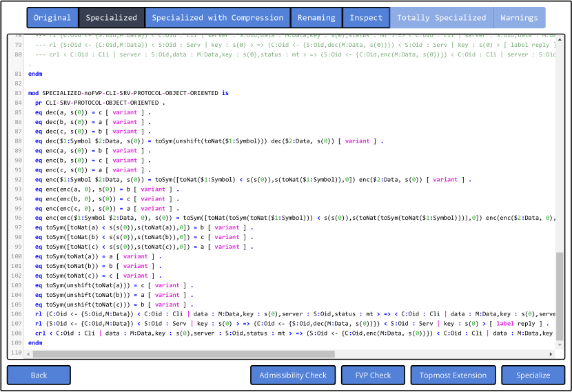
Figure 10: Specialized client-server communication protocol before the compression phase.

Figure 11: Specialized client-server communication protocol after the compression phase.

Inspection mode. By activating the inspect tab, Presto shows detailed information of the specialization process that can be particularly useful for a user who wants to experiment with different specializations for analysis and verification purposes. Specifically, for each iteration $i$ of the EqNPE^U algorithm (invoked in Line 4 of Algorithm 1), Presto shows all of the leaves (term variants) in the deployed fV-narrowing trees for the calls that were specialized at the iteration $i$, together with their corresponding computed substitution (i.e., the substitution component of a term variant). Also, thanks to the interconnection with the narrowing stepper Narval [Alpuente et al., 2019b], each fV-narrowing tree computed at iteration $i$ can be graphically visualized and interactively navigated. This is automatically done by simply selecting the desired tree root term to be expanded from the displayed list of calls that were specialized at any iteration (including the last one). This can be done by simply clicking the hyperlink associated with the desired call. By doing this, the user can perform a fine-grained and stepwise inspection of all narrowing steps, computation of equational unifiers, and interactive exploration of different representations of Maude’s narrowing and rewriting search spaces (tree-based or graph-based, source-level or meta-level). For instance, Figure 12 shows that, at iteration 1, a fV-narrowing tree was expanded whose root term is the specialized call dec(M:Data,s(0)) (Line 47). The root can be narrowed to the leaf a (Line 48) with the computed substitution {M $\mapsto$ b} (Line 49), which allows the resultant equation dec(b,s(0)) = a to be generated (Line 50). Furthermore, Figure 13 shows (a fragment of) the fV-narrowing tree for the specialized call dec(M:Data,s(0)) of Line 47 that has been generated by the Narval system.

Figure 12: Inspecting the specialization process.

Figure 13: Fragment of the fV-narrowing tree for dec(M:Data,s(0)).

Topmost extension transformation. The topmost extension transformation of Section 3.2 has been fully implemented in Presto. Since the topmost property is not required to perform the partial evaluation, it can be applied either ex-ante to the original input program (and it is preserved by the specialization) or ex-post to the specialized program. The transformation enables narrowing-based search reachability for all topmost modulo $Ax$ programs, and particularly for object-oriented specifications. Reachability goals can be solved in Presto through the connection to the Narval system [Alpuente et al., 2019b], which provides a graphical environment for symbolic analysis in Maude. This feature is illustrated in the system quick start guide.

Finite Variant Property and Strong irreducibility checkers. Presto includes a FVP checker for equational theories that is based on the checking procedure described in [Meseguer, 2015]. All of the theories that satisfy the FVP can be specialized by using the unfolding operator $\mathcal{U}_{\mathit{FVP}}$ instead of the typically costlier operator $\mathcal{U}_{\overline{\mathit{FVP}}}$. As discussed in Section 3, the checker implements a semi-decidable procedure that terminates when the FVP holds for the equational theory under examination. If the FVP does not hold, the user has to manually stop the checking process or wait for the time-out; otherwise, the process would produce an infinite number of most general variants for some terms. For instance, consider the Client-Server Communication Protocol with FVP that is available in the Presto preloaded examples. This Maude specification is a slight mutation of the client-server communication protocol of Example 9 that models the Caesar cypher by using a finite variant equational theory. By clicking the Check FVP button, the checking process starts and, in this case, the check succeeds since the flat terms associated with the program operators have only a finite number of most general variants, as illustrated in Figure 14. Hence, the specification could be safely specialized by using the $\mathcal{U}_{\mathit{FVP}}$ unfolding operator without the risk of jeopardizing termination.

Figure 14: FVP checking of the Client-Server Communication Protocol with FVP.

Moreover, Presto  implements an efficient checker for the $(\vec{E},B)$-strong irreducibility of the left-hand side of the rewrite rules of the input program. As discussed at the end of Section 4.2, strong irreducibility is an essential requirement for the completeness of the specialization algorithm. Figure 15 illustrates the outcome of the strong irreducibility check for a variant of the Client-Server Communication Protocol with FVP that includes the rewrite rule

rl [C:CliName,S:ServName,enc(Q:Message,K:Nat),K:Nat,mt]
                      => (S:ServName <- {C:CliName,enc(Q:Message, K:Nat)}) &
                         [C:CliName,S:ServName,Q:Message,K:Nat,mt] .

Note that the check fails due to the narrowable subterm enc(Q:Message, K:Nat) occurring in the left-hand side of the considered rule.

Figure 15: Strong irreducibility failure for a variant of the Client-Server Communication Protocol with FVP.

Iterative specialization. Presto can be automatically re-applied to any generated specialization in an iterative manner. After completing a given specialization for a rewrite theory, the user can perform a further specialization process to re-specialize the given outcome by using a distinct unfolding operator. This is achieved by simply pressing the Specialize button again, which is directly displayed after the specialization and avoids the need to reload the initial web input form to manually enter the intermediate program to be re-specialized. As shown in [Alpuente et al., 2021a], this feature is particularly useful in the case when a given input rewrite theory $\mathcal{R}$ must be specialized using $\mathcal{U}_{\overline{\mathit{FVP}}}$, since its equational theory does not satisfy the FVP, while the resulting specialization $\mathcal{R}^{\prime}$ hosts an equational theory that does satisfy the FVP so that $\mathcal{R}^{\prime}$ can be further specialized by using the $\mathcal{U}_{\mathit{FVP}}$ operator. For a detailed session with Presto that illustrates this feature, we refer to the Presto quick start guide.

Figure 16: Total evaluation of the Client-Server Communication Protocol with FVP.

Total evaluation. This feature provides a slightly modified version of the unfolding operator $\mathcal{U}_{\mathit{FVP}}$ that implements the total evaluation transformation of [Meseguer, 2020] for sufficiently complete equational theories that have the FVP. By means of a suitable sort downgrading, which is described in [Meseguer, 2020], function calls always generate values and cannot be stuck in an intermediate, partial result. In this scenario, unfolding can safely rule out variants that are not constructor terms. This means that all of the specialized calls get totally evaluated and the maximum compression is achieved, thereby dramatically reducing the search space for the construction of the specialized theories as shown in [Alpuente et al., 2021a].

For instance, the specialized rewrite theory Client-Server Communication Protocol with FVP can be totally evaluated into the extremely compact rewrite theory of Figure 16, which does not include any equation. Actually, all calls to the encryption and decryption functions have been totally evaluated, and their values have been hard-coded into their place in the specialized rewrite rules.

7 Experimental Evaluation of Presto

Program	${Size}$	$\#Rews_{\mathcal{R}}$	$\#Rews_{\mathcal{R}^{\prime}}$	Reduction	$T_{\mathcal{R}}$ (ms)	$T_{\mathcal{R}^{\prime}}$ (ms)	Speedup
	25K	650,012	100,002	84.62%	47	15	3.13
Cli-Srv	100K	2,600,115	400,002	84.62%	261	87	3.00
	1M	26,000,100	4,000,002	84.62%	5,630	2,434	2.31
	25K	8,900,012	100,002	98.88%	780	14	55.71
Cli-Srv-Mod	100K	35,600,115	400,002	98.88%	3,723	87	42.79
	1M	356,000,100	4,000,002	98.88%	56,087	2,399	23.38
	1M	302,000,000	2,000,000	99.34%	21,163	584	36.24
Diffie-Hellman	5M	1,510,000,000	10,000,000	99.34%	104,959	3,087	34.00
	10M	3,020,000,000	20,000,000	99.34%	207,189	6,361	32.57
	1M	12,000,000	4,000,000	66.67%	976	339	2.88
Cli-Srv-FVP	5M	60,000,000	20,000,000	66.67%	4,866	1,680	2.90
	10M	120,000,000	40,000,000	66.67%	10,305	3,310	3.11
	1M	1,575,500,000	1,500,000	99.90%	67,646	546	123.89
Handshake-KMP	5M	7,877,500,000	7,500,000	99.90%	336,147	3,042	110.50
	10M	15,755,000,000	15,000,000	99.90%	655,962	6,077	107.94
	25K	1,500,000	200,000	86.67%	118	36	3.28
Cond-Cli-Srv-OO	100K	6,000,000	800,000	86.67%	405	125	3.24
	1M	60,000,000	8,000,000	86.67%	4,017	1,250	3.21
	1M	695,000,000	1,000,000	99.86%	48,048	822	58.45
Cond-Diffie-Hellman-OO	5M	3,475,000,000	5,000,000	99.86%	249,551	4,060	61.47
	10M	6,950,000,000	10,000,000	99.86%	526,527	8,107	64.95
	1M	3,833,996,167	1,000,000	99.97%	189,779	873	217.39
Cond-Handshake-KMP-OO	5M	19,169,996,167	5,000,000	99.97%	923,511	4,330	213.28
	10M	38,339,996,167	10,000,000	99.97%	1,886,552	8,898	212.02

Table 1: Experimental results for the specialization of rewrite theories with Presto.

Table 1 contains the experiments that we have performed with Presto  using an Intel Xeon E5-1660 3.3GHz CPU with 64 GB RAM running Maude v3.0 and considering the average of ten executions for each test. These experiments, together with the source code of all of the examples are also publicly available at Presto’s website.

We have considered the following benchmark programs: Cond-Cli-Srv-OO, the conditional, object-oriented, client-server communication protocol of Example 9; Cli-Srv, a re-encoding of Cond-Cli-Srv-OO that does not use either Maude built-in object-oriented features or conditional rules; Cli-Srv-Mod, a variant of Cli-Srv where we introduce an extra function (i.e., the mod function that computes the remainder of the integer division) in the underlying equational theory that is commonly used in protocol specification and makes the key generation heavier; Cli-Srv-FVP, a variant of Cli-Srv for one-symbol messages whose equational theory meets the FVP and differs from the one in Example 10 in using Presburger’s encoding for natural numbers; Diffie-Hellman, the well-known network protocol for safely sharing keys between two nodes over an untrusted channel; Cond-Diffie-Hellman-OO, a conditional, object-oriented specification of the Diffie-Hellman protocol; Handshake-KMP, an unconditional rewrite theory that specifies a simple handshake protocol in which a client sends an arbitrary long and noisy message M to a server. The handshake succeeds if the server can recognize a secret handshake sequence P inside the client message M by matching P against M via the well-known KMP string matching algorithm; and Cond-Handshake-KMP-OO, a conditional, object-oriented version of Handshake-KMP.

As for the experiments with Cli-Srv, Cli-Srv-Mod and Cond-Cli-Srv-OO, we considered input messages of three different sizes: from twenty-five thousand symbols to one million symbols. This cannot be done for Cli-Srv-FVP since it encodes one-symbol messages, and, hence, we cannot use this parameter for benchmarking purposes. Similarly, Handshake-KMP and Cond-Handshake-KMP-OO consider fixed-size messages of 350 symbols, while Diffie-Hellman and Cond-Diffie-Hellman-OO are specialized w.r.t. fixed-size keys (modelled as natural numbers obtained though exponentiation). For these experiments, we use as benchmark parameter the number of client requests sent over a time-bounded period of time. We considered one, five, and ten millions requests. The column Size in Table 1 indicates either the message length parameter or the number of client requests according to the benchmark program considered.

For each experiment, we executed the original specification $\mathcal{R}$ and the specialized one $\mathcal{R}^{\prime}$ on the very same input states, and we recorded the following data: the execution times (in ms) $T_{\mathcal{R}}$ and $T_{\mathcal{R}}^{\prime}$, the total number of rewrites $\#Rews_{\mathcal{R}}$ and $\#Rews_{\mathcal{R}^{\prime}}$, the percentage of reduction in terms of number of rewrites, and the specialization speedup computed as the ratio $T_{\mathcal{R}}/T_{\mathcal{R}^{\prime}}$.

Our figures show that the specialized rewrite theories achieve a significant improvement in execution time when compared to the original theory, with an average speedup for these benchmarks of $59.24$. Particularly remarkable is the performance improvement of the Cond-Handshake-KMP-OO which reaches two orders of magnitude for the case when the specialized maximal calls within the rewrite theory partially instantiate the input pattern and input message. Such an impressive performance is largely due to the compression phase of the specialization algorithm that, in this case, completely deconditionalizes the rewrite rules, thereby yielding as outcome a faster, unconditional rewrite theory. This does not happen for Cond-Cli-Srv-OO which exhibits a smaller speedup. For this benchmark, complete deconditionalization cannot be achieved as shown in Example 9, hence some heavy conditional computations are kept in the specialized program as well.

We note that none of these specializations could be performed by using our earlier partial evaluator Victoria, which cannot handle rewrite theories but only equational theories. Thus, the specialization of rewrite theories supported by Presto could not be achieved in Victoria unless a complex hack is introduced not only at the level of the theory signature but also by providing a suitable program infrastructure that simulates rewrite rule nondeterminism through deterministic, equational evaluation.

We do not benchmark the specialization times since they are almost negligible (for most cases $<$100 ms). Nonetheless, we compared the performance of the unfolding operators $\mathcal{U}_{\mathit{FVP}}$ and $\mathcal{U}_{\overline{FVP}}$, when both can be applied in the specialization process (i.e., when the rewrite theory to be specialized includes a finite variant equational theory). The most significant difference appears in the Cli-Srv-FVP theory, where NPER${}^{\mathcal{U}_{\mathit{FVP}}}$ is 56% faster (on average) than NPER${}^{\mathcal{U}_{\overline{FVP}}}$. This figure is expected and favors the use of $\mathcal{U}_{\mathit{FVP}}$ whenever it is possible since it avoids any overhead caused by homeomorphic embedding checks performed by $\mathcal{U}_{\overline{FVP}}$. Finally, we benchmarked the symbolic execution of long-winded reachability goals in rewrite theories that include a finite variant equational theory such as the pathological theory of Example 11. The achieved improvement is also striking, with an average speedup of $16.46$.

Let us finally discuss how Presto compares in practice with existing on-line specialization systems with related transformation power. A narrowing-based partial evaluator for the lazy functional logic language Curry is described in [Hanus and Peemöller, 2014, Peemöller, 2017] whose implementation can be seen as an instance of the generic narrowing-based partial evaluation framework of [Alpuente et al., 1998b]. This system improves a former prototype in [Albert et al., 2002] by taking into account (mutually recursive) let expressions and non-deterministic operations, while the PE system of [Albert et al., 2002] was restricted to confluent programs. Obviously, the protocol benchmarks in this paper cannot be directly specialized by using Curry’s partial evaluator since neither evaluation modulo algebraic axioms nor concurrency are supported by Curry’s partial evaluator; this would require artificially rewriting the program code so that any comparison would be meaningless. In the opposite direction, Presto cannot manage the specialization of higher-order functions that is achieved by [Hanus and Peemöller, 2014] since RWL is not a higher-order logic. Furthermore, our partial evaluator cannot deal with many other important Curry features such as monadic I/O or encapsulated search. In order to provide some evidence of how Presto performs on classical specialization examples, we reproduced the standard kmp-match test (i.e., without using any algebraic axioms), and we benchmarked the speed and specialization that is achieved by Presto on this program. This example is particularly interesting because it is a kind of transformation that neither (conventional) PE nor deforestation can perform automatically while conjunctive partial deduction of logic programs and positive supercompilation of functional programs can pass the test [Alpuente et al., 1998a, Jørgensen et al., 1996]. The speedup achieved by Presto on this test for an input list with 500,000 elements is $58$, which is comparable to the speedup of the last release of Victoria (actually, the KMP specialized programs that are generated by Presto and Victoria are essentially the same and they both yield an optimal specialized string matcher). Curry’s partial evaluator also produces an optimal KMP specialization and the achieved speedup for input lists of $500,000$ elements is $12.22$, which is obtained by using an unlimited unfolding strategy that, however, may risk nontermination [Peemöller, 2017]. The corresponding specialization time of Curry’s partial evaluator reported in [Peemöller, 2017] is $1.61$ seconds.

We compared the specialization times achieved by Presto in comparison to Victoria as follows. In order to reduce the noise on the small time for a single specialization, we benchmarked the total specialization time for a loop consisting of $1000$ specializations of the KMP program, and then we divided the accumulated specialization time by $1000$. The resulting specialization times of Victoria and Presto  are $6.6$ ms and $5.6$ ms, respectively, which shows that Presto outperforms Victoria with a performance improvement of $15\%$. This is noteworthy since the implementation of Presto is considerably more ambitious, and it provides much greater coverage compared to the simpler approach of Victoria.

8 Conclusion

The use of logic programming and narrowing for system analysis has been advocated since the narrowing-based NRL protocol analyzer [Meadows, 1996], which was developed in Prolog. In this article, we have shown that concurrent software analysis is a promising new application area for narrowing-based program specialization. We believe that Maude’s partial evaluator Presto  is not only relevant for the (multi-paradigm) logic programming community working on source code optimization, but it can also be a valuable tool for anyone who is interested in the symbolic analysis and verification of concurrent systems. The main reason why Presto is so effective in this area is that it not only achieves huge speedup for important classes of rewrite theories, but it can also cut down an infinite (folding variant) narrowing space to a finite one for the underlying equational theory $\mathcal{E}$. By doing this, any $\mathcal{E}$-unification problem can be finitely solved and symbolic, narrowing-based analysis with rules $R$ modulo $\mathcal{E}$ can be effectively performed. Moreover, in many cases, the specialization process transforms a rewrite theory whose operators obey algebraic axioms, such as associativity, commutativity, and unity, into a much simpler rewrite theory with the same semantics and no structural axioms so that it can be run in an independent rewriting infrastructure that does not support rewriting or narrowing modulo axioms. Finally, some costly analyses that may require significant (or even unaffordable) resources in both time and space, can now be safely and effectively performed.

The current specialization system goes beyond the scope of the original NPER framework of [Alpuente et al., 2022], which only works on unconditional rewrite theories. Presto is now “feature complete” and stable. As such, it is not only suitable for experimental use but also for production use. Since Presto is a fully automatic online specializer, its usage is simple and accessible for Maude users, and its interactive features make the specialization process fully checkable. For instance, the user can simply click on a specialized call to see its unfolding tree and all of the derived resultants.

Besides the applications outlined in this article, further applications could benefit from the optimization of variant generation that is achieved by Presto. For instance, an important number of applications (and tools) are currently based on narrowing-based variant generation: for example, the protocol analyzers Maude-NPA [Escobar et al., 2009] and Tamarin  [Meier et al., 2013], Maude debuggers and program analyzers  [Alpuente et al., 2016, Alpuente et al., 2012, Alpuente et al., 2014a], termination provers, variant-based satisfiability checkers, coherence and confluence provers, and different applications of symbolic reachability analysis [Durán et al., 2020a]. Also, as stated in [Leuschel and Lehmann, 2000], there are big advantages for using the partial deduction approach to model checking due to the built-in support of logic programming for non-determinism and unification. This approach might also be of great value in the optimization of Maude’s logical model checkers for infinite-state systems, where narrowing, equational unification, and equational abstractions play a primary role [Escobar and Meseguer, 2007, Bae and Meseguer, 2015]. We plan to investigate this in future research.

We also plan to implement new unfolding operators in Presto that can achieve the total evaluation of [Meseguer, 2020] for the case of equational theories that are sufficiently complete modulo axioms but do not have the FVP. This requires significant research effort since total evaluation relies on the notion of constructor variant and there does not exist in the literature a finite procedure to compute a finite, minimal, and complete set of most general constructor variants for theories that do not have the FVP, even if this set exists. Another interesting strand for further research is dealing with the recently proposed Maude strategy language [Durán et al., 2020a] in program specialization.

Appendix A Proofs of Technical Results

Theorem 3.1 (strong completeness of topmost extension). Let $\mathcal{R}=(\Sigma,E\uplus B,R)$ be a topmost modulo $Ax$ rewrite theory, with $Ax\in B$, and let $\mathcal{E}=(\Sigma,E\uplus B)$ be a convergent, finite variant equational theory where $B$-unification is decidable. Let $\hat{\mathcal{R}}=(\hat{\Sigma},E\uplus B,\hat{R})$ be the topmost extension of $\mathcal{R}$ and let $G=(\exists X)\;t\longrightarrow^{*}t^{\prime}$ be a reachability goal in $\mathcal{R}$. If $\sigma$ is a solution for $G$ in $\mathcal{R}$, then there exists a term $t^{\prime\prime}$ such that $\{t\}\leadsto_{\hat{R},\mathcal{E}}^{*}\{t^{\prime\prime}\}$ with computed substitution $\theta$ and $\sigma=_{\mathcal{E}}\theta\eta$, where $\eta$ is an $\mathcal{E}$-unifier of $t^{\prime\prime}$ and $t^{\prime}$.

Proof A.1.

Let $\mathcal{R}=(\Sigma,E\uplus B,R)$ be a topmost modulo $Ax$ rewrite theory and $Ax\in B$, and let $\mathcal{E}=(\Sigma,E\uplus B)$ be a convergent, finite variant equational theory where $B$-unification is decidable.

Let $\hat{\mathcal{R}}=(\hat{\Sigma},E\uplus B,\hat{R})$ be the topmost extension of $\mathcal{R}$. Let $G=((\exists X)\;t\longrightarrow^{*}t^{\prime})$ be a reachability goal for $\mathcal{R}$. If $\sigma$ is a solution for $G$ in $\mathcal{R}$, then $t\sigma\rightarrow_{R,\mathcal{E}}^{*}t^{\prime}\sigma$. By Proposition 3.1, we have $\{t\}\sigma\rightarrow_{\hat{R},\mathcal{E}}^{*}\{t^{\prime}\}\sigma$, which means that $\sigma$ is a solution in $\hat{\mathcal{R}}$ for $\hat{G}=((\exists X)\;\{t\}\longrightarrow^{*}\{t^{\prime}\})$.

Since $\mathcal{E}=(\Sigma,E\uplus B)$ is a convergent, finite variant equational theory where $B$-unification is decidable, $\mathcal{E}$-unification is decidable. Furthermore, since $\hat{\mathcal{R}}$ is topmost and $\mathcal{E}$-unification is decidable, $\leadsto_{\hat{R},\mathcal{E}}$ is complete and thus there exist $\{t\}\leadsto_{\hat{R},\mathcal{E}}^{*}\{t^{\prime\prime}\}$ with a computed substitution $\theta$ and an $\mathcal{E}$-unifier $\eta$ such that $\theta\eta=_{\mathcal{E}}\sigma$.

Proposition 3.1 (correctness and completeness of the topmost extension). Let $\mathcal{R}=(\Sigma,E\uplus B,R)$, with $\mathcal{E}=(\Sigma,E\uplus B)$, be a topmost modulo $Ax$ theory and let $\hat{\mathcal{R}}$ be the topmost extension of $\mathcal{R}$. For any terms $t_{i}$ and $t_{f}$ of sort $\mathit{Config}$, $t_{i}\rightarrow_{R,\mathcal{E}}^{*}t_{f}$ iff $\{t_{i}\}\rightarrow_{\hat{R},\mathcal{E}}^{*}\{t_{f}\}$.

Proof A.2.

The case when $Ax=$ACU has been stated in Lemma 5.3 of [Meseguer and Thati, 2007]. Here, we prove the case when $Ax=$AC, which involves two extension rewrite rules, namely, $(\{X\otimes\lambda\}\Rightarrow\{X\otimes\rho\}\mbox{ if }C)$ and $(\{\lambda\}\Rightarrow\{\rho\}\mbox{ if }C)$. The remaining cases are straightforward adaptations of the following proof scheme.

We have to prove the following two implications for the case when $Ax=$AC:

$(\rightarrow)$

for any term $t_{i}$ and $t_{f}$ of sort $\mathit{Config}$, $t_{i}\rightarrow_{R,\mathcal{E}}^{*}t_{f}$ implies $\{t_{i}\}\rightarrow_{\hat{R},\mathcal{E}}^{*}\{t_{f}\}$;

$(\leftarrow)$

for any term $t_{i}$ and $t_{f}$ of sort $\mathit{Config}$, $\{t_{i}\}\rightarrow_{\hat{R},\mathcal{E}}^{*}\{t_{f}\}$ implies $t_{i}\rightarrow_{R,\mathcal{E}}^{*}t_{f}$.

$(\rightarrow)$

Assume that $t_{i}\rightarrow_{R,\mathcal{E}}^{*}t_{f}$, where $t_{i}$ and $t_{f}$ are arbitrary terms of sort $\mathit{Config}$. Then, $t_{i}\rightarrow_{R,\mathcal{E}}^{*}t_{f}$ has the form

$$t_{i}=t_{0}\rightarrow_{R,\mathcal{E}}\ldots\rightarrow_{R,\mathcal{E}}t_{n-1}\rightarrow_{R,\mathcal{E}}t_{n}=t_{f},\mbox{for some natural number }n\geq 0.$$

We proceed by induction on the length $n$ of the rewriting sequence $t_{i}\rightarrow_{R,\mathcal{E}}^{*}t_{f}$.

$n=0.$ Immediate since there are no rewrite steps.

$n>0.$ By induction hypothesis, we have

$$t_{i}=t_{0}\rightarrow_{R,\mathcal{E}}^{*}t_{n-1}\mbox{ implies }\{t_{i}\}=\{t_{0}\}\rightarrow_{\hat{R},\mathcal{E}}^{*}\{t_{n-1}\}.$$ (3)

Thus, in order to prove $(\rightarrow)$, we just need to show

$$\{t_{n-1}\}\rightarrow_{\hat{R},\mathcal{E}}\{t_{n}\},$$ (4)

whenever $t_{n-1}\rightarrow_{R,\mathcal{E}}t_{n}$. The computation step $t_{n-1}\rightarrow_{R,\mathcal{E}}t_{n}$ in the rewrite theory $\mathcal{R}$ can be expanded into the following rewrite sequence

$$t_{n-1}\stackrel{{\scriptstyle r,\sigma,w}}{{\rightarrow}}_{\!\!R,B}\tilde{t}_{n-1}\rightarrow_{\vec{E},B}^{*}\tilde{t}_{n-1}\!\downarrow_{\vec{E},B}=t_{n}$$

where $r=(\lambda\>\Rightarrow\>\rho\ \mbox{if}\ C)\in R$. Here, we distinguish two cases according to the value of the position $w\in Pos(t_{n-1})$: $w=\Lambda$ and $w\neq\Lambda$.

$(w=\Lambda)$ In this case, $t_{n-1}=_{B}\lambda\sigma$ and $\tilde{t}_{n-1}=_{B}\rho\sigma$ by the definition of ${\rightarrow}_{R,B}$. Furthermore, since $\mathcal{R}$ is topmost modulo $Ax$, $\lambda\sigma$ and $\rho\sigma$ have sort $\mathit{Config}$. From these facts, it immediately follows that

$$\{t_{n-1}\}=_{B}\{\lambda\sigma\}\stackrel{{\scriptstyle\hat{r},\sigma,\Lambda}}{{\rightarrow}}_{\!\!\hat{R},B}\{\rho\sigma\}=_{B}\{\tilde{t}_{n-1}\}\rightarrow_{\vec{E},B}^{*}\{\tilde{t}_{n-1}\}\!\downarrow_{\vec{E},B}=\{t_{n}\}$$

with $\hat{r}=\{\lambda\}\Rightarrow\{\rho\}\mbox{ if }C\in\hat{R}$. Hence, $\{t_{n-1}\}\rightarrow_{\hat{R},\mathcal{E}}\{t_{n}\}$ when $w=\Lambda$.

$(w\neq\Lambda)$ Since $\mathcal{R}$ is topmost modulo $Ax$ and $w\neq\Lambda$, there exist $u_{i}\in\mathcal{T}_{\Sigma}(\mathcal{X})$ of sort $\mathit{Config}$, $i=1,\ldots,k$, with $k>1$ such that

$$t_{n-1}=u_{1}\otimes\ldots\otimes u_{k}$$

and $t_{n-1}\in\mathcal{T}_{{\Sigma}}(\mathcal{X})$ of sort $\mathit{Config}$. Now, since $t_{n-1}\stackrel{{\scriptstyle r,\sigma,w}}{{\rightarrow}}_{\!\!R,B}\tilde{t}_{n-1}\rightarrow_{\vec{E},B}^{*}t_{n}$, with $Ax=AC$ and $r=(\lambda\Rightarrow\rho\mbox{ if }C)$,

$$t_{n-1}=u_{1}\otimes\ldots\otimes u_{k} =_{AC}u_{\pi(1)}\otimes\ldots\otimes u_{\pi(m)}\otimes\lambda\sigma$$

$$\stackrel{{\scriptstyle r,\sigma,w}}{{\rightarrow}}_{\!\!R,B}u_{\pi(1)}\otimes\ldots\otimes u_{\pi(m)}\otimes\rho\sigma\rightarrow_{\vec{E},B}^{*}t_{n}$$

where $1\leq m\leq k-1$, and $\pi\colon\{1,...,m\}\to\{1,\ldots,k\}$ is an injective function that selects a permutation of $m$ $u_{i}$’s within $u_{1}\otimes\ldots\otimes u_{k}$. Hence, we can build the following rewrite sequence

$$\{t_{n-1}\}=\{u_{1}\otimes\ldots\otimes u_{k}\} =_{AC}\{u_{\pi(1)}\otimes\ldots\otimes u_{\pi(m)}\otimes\lambda\sigma\}$$

$$\stackrel{{\scriptstyle\hat{r},\hat{\sigma},\Lambda}}{{\rightarrow}}_{\!\!\hat{R},B}\{u_{\pi(1)}\otimes\ldots\otimes u_{\pi(m)}\otimes\rho\sigma\}\rightarrow_{\vec{E},B}^{*}\{t_{n}\}$$

with $\hat{\sigma}=\sigma\cup\{X\mapsto u_{\pi(1)}\otimes\ldots\otimes u_{\pi(m)}\}$, and $\hat{r}=(\{X\otimes\lambda\}\Rightarrow\{X\otimes\rho\}\mbox{ if }C)\in\hat{R}$. This proves that $\{t_{n-1}\}\rightarrow_{\hat{R},\mathcal{E}}\{t_{n}\}$ also in the case when $w\neq\Lambda$.

Finally, by using the induction hypothesis 3 and the rewrite step 4, we easily derive the implication $(\rightarrow)$.

$(\leftarrow)$

Assume that $\{t_{i}\}\rightarrow_{\hat{R},\mathcal{E}}^{*}\{t_{f}\}$, where $t_{i}$ and $t_{f}$ are arbitrary terms of sort $\mathit{Config}$. Then, $\{t_{i}\}\rightarrow_{\hat{R},\mathcal{E}}^{*}\{t_{f}\}$ is of the form

$$\{t_{i}\}=\{t_{0}\}\rightarrow_{\hat{R},\mathcal{E}}\ldots\rightarrow_{\hat{R},\mathcal{E}}\{t_{n-1}\}\rightarrow_{\hat{R},\mathcal{E}}\{t_{n}\}=\{t_{f}\}$$

for some natural number $n\geq 0.$ We proceed by induction on the length $n$ of the computation $\{t_{i}\}\rightarrow_{\hat{R},\mathcal{E}}^{*}\{t_{f}\}$.

$n=0.$ Immediate, since there are no rewrite steps.

$n>0.$ This case is analogous to the proof of the inductive step of Case $(\rightarrow)$. By induction hypothesis, we have

$$\{t_{i}\}=\{t_{0}\}\rightarrow_{\hat{R},\mathcal{E}}^{*}\{t_{n-1}\}\mbox{ implies }t_{i}=t_{0}\rightarrow_{R,\mathcal{E}}^{*}t_{n-1}.$$ (5)

Therefore, it suffices to show that $t_{n-1}\rightarrow_{R,\mathcal{E}}^{*}t_{n}$ and combine this result with the induction hypothesis to finally prove Case $(\leftarrow)$.

By hypothesis, $\{t_{n-1}\}\rightarrow_{\hat{R},\mathcal{E}}\{t_{n}\}$, which can be expanded into the following rewrite sequence

$$\{t_{n-1}\}\stackrel{{\scriptstyle\hat{r},\hat{\sigma},\Lambda}}{{\rightarrow}}_{\!\!\hat{R},B}\{\tilde{t}_{n-1}\}\rightarrow_{\vec{E},B}^{*}\{\tilde{t}_{n-1}\}\!\downarrow_{\vec{E},B}=\{t_{n}\}$$ (6)

where $\hat{r}\in\hat{R}$, and $\{t_{n-1}\},\{\tilde{t}_{n-1}\},\{t_{n}\}\in\mathcal{T}_{\hat{\Sigma}}(\mathcal{X})$ of sort $\mathit{State}$. Observe that the first rewrite step of the rewrite sequence (6) must occur at position $\Lambda$, since the rewrite theory $\hat{\mathcal{R}}$ is topmost.

Here, we distinguish two cases according to the form of the rewrite rule $\hat{r}\in\hat{R}$ applied in $\{t_{n-1}\}\stackrel{{\scriptstyle\hat{r},\hat{\sigma},\Lambda}}{{\rightarrow}}_{\!\!\hat{R},B}\{\tilde{t}_{n-1}\}$.

By Definition 2, $\hat{r}$ is either $\{\lambda\}\Rightarrow\{\rho\}\mbox{ if }C$ or $\{X\otimes\lambda\}\Rightarrow\{X\otimes\rho\}\mbox{ if }C$, as $Ax=AC$ and $\{t_{n-1}\},\{\tilde{t}_{n-1}\}\in\mathcal{T}_{\hat{\Sigma}}(\mathcal{X})$ of sort $\mathit{State}$.

Case $(\hat{r}=(\{\lambda\}\Rightarrow\{\rho\}\mbox{ if }C))$. In this case, $\{t_{n-1}\}\stackrel{{\scriptstyle\hat{r},\hat{\sigma},\Lambda}}{{\rightarrow}}_{\!\!\hat{R},B}\{\tilde{t}_{n-1}\}$ assumes the following form:

$$\{t_{n-1}\}=_{AC}\{\lambda\sigma\}\stackrel{{\scriptstyle\hat{r},\sigma,\Lambda}}{{\rightarrow}}_{\!\!\hat{R},B}\{\rho\sigma\}=_{AC}\{{\tilde{t}_{n-1}}\}.$$

Now, by Definition 2, $\lambda\sigma$ and $\rho\sigma$ are terms of sort $\mathit{Config}$; thus, we can also apply $r=(\lambda\Rightarrow\rho\mbox{ if }C)\in R$ to $\lambda\sigma$, thereby obtaining the following computation

$$t_{n-1}=_{AC}\lambda\sigma\stackrel{{\scriptstyle r,\sigma,\Lambda}}{{\rightarrow}}_{\!\!R,B}\rho\sigma\rightarrow_{\vec{E},B}^{*}(\rho\sigma\downarrow_{\vec{E},B})=t_{n}$$

which corresponds to $t_{n-1}\rightarrow_{R,\mathcal{E}}t_{n}$ when $\hat{r}=(\{\lambda\}\Rightarrow\{\rho\}\mbox{ if }C)$.

Case $(\hat{r}=(\{X\otimes\lambda\}\Rightarrow\{X\otimes\rho\}\mbox{ if }C))$. In this case, $\{t_{n-1}\}\stackrel{{\scriptstyle\hat{r},\hat{\sigma},\Lambda}}{{\rightarrow}}_{\!\!\hat{R},B}\{\tilde{t}_{n-1}\}$ must have the following form:

$$\{t_{n-1}\}=_{AC}\{u\otimes\lambda\hat{\sigma}\}\stackrel{{\scriptstyle\hat{r},\hat{\sigma},\Lambda}}{{\rightarrow}}_{\!\!\hat{R},B}\{u\otimes\rho\hat{\sigma}\}=_{AC}\{\tilde{t}_{n-1}\}$$

where $u,\lambda\hat{\sigma},\rho\hat{\sigma}\in\mathcal{T}(\Sigma,\mathcal{V})_{\mathit{Config}}$, and $\hat{\sigma}=\{X\mapsto c\}\cup\sigma$, for some substitution $\sigma$.

Now, by Definition 2, variable $X$ does not occur in either $\lambda$ or $\rho$; this implies that $\lambda\hat{\sigma}=\lambda\sigma$ and $\rho\hat{\sigma}=\rho\sigma$. Therefore, we can construct the following computation:

$$t_{n-1}=_{AC}u\otimes\lambda\hat{\sigma}=u\otimes\lambda\sigma\stackrel{{\scriptstyle r,\sigma,w}}{{\rightarrow}}_{\!\!R,B}u\otimes\rho\sigma=u\otimes\rho\hat{\sigma}=_{AC}\tilde{t}_{n-1}\rightarrow_{\vec{E},B}^{*}t_{n}$$

where $r=(\lambda\Rightarrow\rho\mbox{ if }C)\in R$ and $w\in Pos(u\otimes\lambda\sigma)$ is the position of the term $\lambda\sigma$ inside $u\otimes\lambda\sigma$. Hence, $t_{n-1}\rightarrow_{R,\mathcal{E}}t_{n}$ even in the case when $\hat{r}=(\{X\otimes\lambda\}\Rightarrow\{X\otimes\rho\}\mbox{ if }C)$.

References

- [Aguirre et al., 2014] Aguirre, L., Martí-Oliet, N., Palomino, M., and Pita, I. (2014). Conditional Narrowing Modulo in Rewriting Logic and Maude. In Proceedings of the 10th International Workshop on Rewriting Logic and its Applications (WRLA 2014), volume 8663 of Lecture Notes in Computer Science, pages 80–96. Springer.
- [Albert et al., 1998] Albert, E., Alpuente, M., Falaschi, M., and Vidal, G. (1998). Indy User’s Manual. Technical Report DSIC-II/12/98, Department of Computer Systems and Computation, Universitat Politècnica de València.
- [Albert et al., 1999] Albert, E., Alpuente, M., Hanus, M., and Vidal, G. (1999). A Partial Evaluation Framework for Curry Programs. In Proceedings of the 6th International Conference on Logic for Programming, Artificial Intelligence and Reasoning (LPAR 1999), volume 1705 of Lecture Notes in Computer Science, pages 376–395. Springer.
- [Albert et al., 2009] Albert, E., Gallagher, J. P., Gómez-Zamalloa, M., and Puebla, G. (2009). Type-based Homeomorphic Embedding for Online Termination. Information Processing Letters, 109(15):879–886.
- [Albert et al., 2002] Albert, E., Hanus, M., and Vidal, G. (2002). A Practical Partial Evaluation Scheme for Multi-Paradigm Declarative Languages. Journal of Functional and Logic Programming, 2002:1–34.
- [Alpuente et al., 2019a] Alpuente, M., Ballis, D., Cuenca-Ortega, A., Escobar, S., and Meseguer, J. (2019a). ACUOS: A High-Performance System for Modular ACU Generalization with Subtyping and Inheritance. In Proceedings of the 16th European Conference on Logics in Artificial Intelligence (JELIA 2019), volume 11468 of Lecture Notes in Computer Science, pages 171–181. Springer.
- [Alpuente et al., 2021a] Alpuente, M., Ballis, D., Escobar, S., Meseguer, J., and Sapiña, J. (2021a). Optimizing Maude Programs via Program Specialization. In Gallagher, J. P., Giacobazzi, R., and López-García, P., editors, Festschrift volume in honor of Manuel Hermenegildo (submitted, invited contribution). Elsevier Science. Available at: http://elp.webs.upv.es/papers/ABEMS20-Festschrift.pdf.
- [Alpuente et al., 2019b] Alpuente, M., Ballis, D., Escobar, S., and Sapiña, J. (2019b). Symbolic Analysis of Maude Theories with Narval. Theory and Practice of Logic Programming, 19(5–6):874–890.
- [Alpuente et al., 2022] Alpuente, M., Ballis, D., Escobar, S., and Sapiña, J. (2022). Optimization of Rewrite Theories by Equational Partial Evaluation. Journal of Logical and Algebraic Methods in Programming, 124.
- [Alpuente et al., 2012] Alpuente, M., Ballis, D., Frechina, F., and Romero, D. (2012). Backward Trace Slicing for Conditional Rewrite Theories. In Proceedings of the 18th International Conference on Logic for Programming, Artificial Intelligence and Reasoning (LPAR 2012), volume 7180 of Lecture Notes in Computer Science, pages 62–76. Springer.
- [Alpuente et al., 2016] Alpuente, M., Ballis, D., Frechina, F., and Sapiña, J. (2016). Debugging Maude Programs via Runtime Assertion Checking and Trace Slicing. Journal of Logical and Algebraic Methods in Programming, 85:707–736.
- [Alpuente et al., 2014a] Alpuente, M., Ballis, D., and Romero, D. (2014a). A Rewriting Logic Approach to the Formal Specification and Verification of Web Applications. Science of Computer Programming, 81:79–107.
- [Alpuente et al., 2019c] Alpuente, M., Ballis, D., and Sapiña, J. (2019c). Static Correction of Maude Programs with Assertions. Journal of Systems and Software, 153:64–85.
- [Alpuente et al., 2020a] Alpuente, M., Ballis, D., and Sapiña, J. (2020a). Efficient Safety Enforcement for Maude Programs via Program Specialization in the ÁTAME system. Mathematics in Computer Science, 14(3):591–606.
- [Alpuente et al., 2010] Alpuente, M., Comini, M., Escobar, S., Iborra, J., and Falaschi, M. (2010). A Compact Fixpoint Semantics for Term Rewriting Systems. Theoretical Computer Science, 411(37):3348–3371.
- [Alpuente et al., 2020b] Alpuente, M., Cuenca-Ortega, A., Escobar, S., and Meseguer, J. (2020b). A Partial Evaluation Framework for Order-Sorted Equational Programs modulo Axioms. Journal of Logical and Algebraic Methods in Programming, 110:1–36.
- [Alpuente et al., 2020c] Alpuente, M., Cuenca-Ortega, A., Escobar, S., and Meseguer, J. (2020c). Order-sorted Homeomorphic Embedding modulo Combinations of Associativity and/or Commutativity Axioms. Fundamenta Informaticae, 177(3–4):297–329.
- [Alpuente et al., 2014b] Alpuente, M., Escobar, S., Espert, J., and Meseguer, J. (2014b). A Modular Order-Sorted Equational Generalization Algorithm. Information and Computation, 235:98–136.
- [Alpuente et al., 2009a] Alpuente, M., Escobar, S., and Iborra, J. (2009a). Termination of Narrowing Revisited. Theoretical Computer Science, 410(46):4608–4625.
- [Alpuente et al., 2008] Alpuente, M., Escobar, S., Meseguer, J., and Ojeda, P. (2008). A Modular Equational Generalization Algorithm. In Proceedings of the 18th International Symposium on Logic-Based Program Synthesis and Transformation (LOPSTR 2008), volume 5438 of Lecture Notes in Computer Science, pages 24–39. Springer.
- [Alpuente et al., 2009b] Alpuente, M., Escobar, S., Meseguer, J., and Ojeda, P. (2009b). Order-Sorted Generalization. Electronic Notes in Theoretical Computer Science, 246:27–38.
- [Alpuente et al., 2021b] Alpuente, M., Escobar, S., Meseguer, J., and Sapiña, J. (2021b). Order-sorted Equational Generalization Algorithm Revisited. Annals of Mathematics and Artificial Intelligence.
- [Alpuente et al., 1997] Alpuente, M., Falaschi, M., Julián, P., and Vidal, G. (1997). Specialization of Lazy Functional Logic Programs. In Proceedings of the ACM SIGPLAN Symposium on Partial Evaluation and Semantics-Based Program Manipulation (PEPM 1997), pages 151–162. Association for Computing Machinery.
- [Alpuente et al., 1998a] Alpuente, M., Falaschi, M., and Vidal, G. (1998a). A Unifying View of Functional and Logic Program Specialization. ACM Computing Surveys, 30(3es):9es.
- [Alpuente et al., 1998b] Alpuente, M., Falaschi, M., and Vidal, G. (1998b). Partial Evaluation of Functional Logic Programs. ACM Transactions on Programming Languages and Systems, 20(4):768–844.
- [Alpuente et al., 2005] Alpuente, M., Lucas, S., Hanus, M., and Vidal, G. (2005). Specialization of Functional Logic Programs based on Needed Narrowing. Theory and Practice of Logic Programming, 5(3):273–303.
- [Bae et al., 2013] Bae, K., Escobar, S., and Meseguer, J. (2013). Abstract Logical Model Checking of Infinite-State Systems Using Narrowing. In Proceedings of the 24th International Conference on Rewriting Techniques and Applications (RTA 2013), volume 21 of Leibniz International Proceedings in Informatics (LIPIcs), pages 81–96. Schloss Dagstuhl - Leibniz-Zentrum für Informatik.
- [Bae and Meseguer, 2015] Bae, K. and Meseguer, J. (2015). Model Checking Linear Temporal Logic of Rewriting Formulas under Localized Fairness. Science of Computer Programming, 99:193–234.
- [Bouchard et al., 2013] Bouchard, C., Gero, K. A., Lynch, C., and Narendran, P. (2013). On Forward Closure and the Finite Variant Property. In Proceedings of the 9th International Symposium on Frontiers of Combining Systems (FroCos 2013), volume 8152 of Lecture Notes in Computer Science, pages 327–342. Springer.
- [Burstall and Darlington, 1977] Burstall, R. M. and Darlington, J. (1977). A Transformation System for Developing Recursive Programs. Journal of the ACM, 24(1):44–67.
- [Cadar and Sen, 2013] Cadar, C. and Sen, K. (2013). Symbolic Execution for Software Testing: Three Decades Later. Communications of the ACM, 56(2):82–90.
- [Clavel et al., 2020] Clavel, M., Durán, F., Eker, S., Escobar, S., Lincoln, P., Martí-Oliet, N., Meseguer, J., Rubio, R., and Talcott, C. (2020). Maude Manual (Version 3.0). Technical report, SRI International Computer Science Laboratory. Available at: http://maude.cs.uiuc.edu.
- [Clavel et al., 2007] Clavel, M., Durán, F., Eker, S., Lincoln, P., Martí-Oliet, N., Meseguer, J., and Talcott, C. (2007). All About Maude: A High-Performance Logical Framework. Springer.
- [Cook and Lämmel, 2011] Cook, W. R. and Lämmel, R. (2011). Tutorial on Online Partial Evaluation. In Proceedings of the IFIP Working Conference on Domain-Specific Languages (DSL 2011), volume 66 of Electronic Proceedings in Theoretical Computer Science, pages 168–180. Open Publishing Association.
- [Cousot and Cousot, 1977] Cousot, P. and Cousot, R. (1977). Abstract Interpretation: A Unified Lattice Model for Static Analysis of Programs by Construction or Approximation of Fixpoints. In Proceedings of the 4th ACM SIGPLAN-SIGACT Symposium on Principles of Programming Languages (POPL 1977), pages 238–252. Association for Computing Machinery.
- [Şerbănută and Roşu, 2006] Şerbănută, T.-F. and Roşu, G. (2006). Computationally Equivalent Elimination of Conditions. In Proceedings of the 17th International Conference on Rewriting Techniques and Applications (RTA 2006), volume 4098 of Lecture Notes in Computer Science, pages 19–34. Springer.
- [De Schreye et al., 1999] De Schreye, D., Glück, R., Jørgensen, J., Leuschel, M., Martens, B., and Sørensen, M. H. (1999). Conjunctive Partial Deduction: Foundations, Control, Algorithms, and Experiments. The Journal of Logic Programming, 41(2-3):231–277.
- [de Waal and Gallagher, 1994] de Waal, D. A. and Gallagher, J. P. (1994). The Applicability of Logic Program Analysis and Transformation to Theorem Proving. In Proceedings of the 12th International Conference on Automated Deduction (CADE 1994), volume 814 of Lecture Notes in Computer Science, pages 207–221. Springer.
- [Durán et al., 2020a] Durán, F., Eker, S., Escobar, S., Martí-Oliet, N., Meseguer, J., Rubio, R., and Talcott, C. (2020a). Programming and Symbolic Computation in Maude. Journal of Logical and Algebraic Methods in Programming, 110.
- [Durán et al., 2008] Durán, F., Lucas, S., and Meseguer, J. (2008). MTT: The Maude Termination Tool (System Description). In Proceedings of the 4th International Joint Conference on Automated Reasoning (IJCAR 2008), volume 5195 of Lecture Notes in Computer Science, pages 313–319. Springer.
- [Durán et al., 2020b] Durán, F., Meseguer, J., and Rocha, C. (2020b). Ground Confluence of Order-Sorted Conditional Specifications Modulo Axioms. Journal of Logical and Algebraic Methods in Programming, 111:100513.
- [Escobar, 2014] Escobar, S. (2014). Functional Logic Programming in Maude. In Specification, Algebra, and Software - Essays Dedicated to Kokichi Futatsugi (SAS 2014), volume 8373 of Lecture Notes in Computer Science, pages 315–336. Springer.
- [Escobar et al., 2009] Escobar, S., Meadows, C., and Meseguer, J. (2009). Maude-NPA: Cryptographic Protocol Analysis Modulo Equational Properties. In Foundations of Security Analysis and Design V (FOSAD 2007/2008/2009 Tutorial Lectures), volume 5705 of Lecture Notes in Computer Science, pages 1–50. Springer.
- [Escobar and Meseguer, 2007] Escobar, S. and Meseguer, J. (2007). Symbolic Model Checking of Infinite-State Systems Using Narrowing. In Proceedings of the 18th International Conference on Term Rewriting and Applications (RTA 2007), volume 4533 of Lecture Notes in Computer Science, pages 153–168. Springer.
- [Escobar et al., 2012] Escobar, S., Sasse, R., and Meseguer, J. (2012). Folding Variant Narrowing and Optimal Variant Termination. The Journal of Logic and Algebraic Programming, 81(7–8):898–928.
- [Fay, 1979] Fay, M. (1979). First Order Unification in an Equational Theory. In Proceedings of the 4th International Conference on Automated Deduction (CADE 1979), pages 161–167. Academic Press, Inc.
- [Gallagher, 1993] Gallagher, J. P. (1993). Tutorial on Specialisation of Logic Programs. In Proceedings of the ACM SIGPLAN Symposium on Partial Evaluation and Semantics-Based Program Manipulation (PEPM 1993), pages 88–98. Association for Computing Machinery.
- [Gallagher and Bruynooghe, 1990] Gallagher, J. P. and Bruynooghe, M. (1990). The Derivation of an Algorithm for Program Specialisation. In Proceedings of the 7th International Conference on Logic Programming (ICLP 1990), pages 732–746. The MIT Press.
- [Garavel et al., 2018] Garavel, H., Tabikh, M., and Arrada, I. (2018). Benchmarking Implementations of Term Rewriting and Pattern Matching in Algebraic, Functional, and Object-Oriented Languages - The 4th Rewrite Engines Competition. In Proceedings of the 12th International Workshop on Rewriting Logic and its Applications (WRLA 2018), volume 11152 of Lecture Notes in Computer Science, pages 1–25. Springer.
- [Hanus, 1994] Hanus, M. (1994). The Integration of Functions into Logic Programming: From Theory to Practice. The Journal of Logic Programming, 19/20:583–628.
- [Hanus, 1997] Hanus, M. (1997). Integration of Declarative Paradigms: Benefits and Challenges. ACM SIGPLAN Notices, 32(1):77–79.
- [Hanus and Peemöller, 2014] Hanus, M. and Peemöller, B. (2014). A Partial Evaluator for Curry. In Proceedings of the 28th International Workshop on (Constraint) Logic Programming (WLP 2014), volume 1335, pages 155–171. CEUR-WS.org.
- [Jones et al., 1993] Jones, N. D., Gomard, C. K., and Sestoft, P. (1993). Partial Evaluation and Automatic Program Generation. Prentice-Hall.
- [Jørgensen et al., 1996] Jørgensen, J., Leuschel, M., and Martens, B. (1996). Conjunctive Partial Deduction in Practice. In Proceedings of the 6th International Symposium on Logic-Based Program Synthesis and Transformation (LOPSTR 1996), volume 1207 of Lecture Notes in Computer Science, pages 59–82. Springer.
- [Leuschel, 1998] Leuschel, M. (1998). On the Power of Homeomorphic Embedding for Online Termination. In Proceedings of the 5th International Symposium on Static Analysis (SAS 1998), volume 1503 of Lecture Notes in Computer Science, pages 230–245. Springer.
- [Leuschel et al., 2006] Leuschel, M., Elphick, D., Varea, M., Craig, S.-J., and Fontaine, M. (2006). The ECCE and LOGEN Partial Evaluators and their Web Interfaces. In Proceedings of the 16th ACM SIGPLAN Symposium on Partial Evaluation and Semantics-Based Program Manipulation (PEPM 2006), pages 88–94. Association for Computing Machinery.
- [Leuschel and Gruner, 2001] Leuschel, M. and Gruner, S. (2001). Abstract Conjunctive Partial Deduction Using Regular Types and Its Application to Model Checking. In Proceedings of the 11th International Symposium on Logic-Based Program Synthesis and Transformation (LOPSTR 2001), volume 2372 of Lecture Notes in Computer Science, pages 91–110. Springer.
- [Leuschel and Lehmann, 2000] Leuschel, M. and Lehmann, H. (2000). Solving Coverability Problems of Petri nets by Partial Deduction. In Proceedings of the 2nd ACM SIGPLAN Conference on Principles and Practice of Declarative Programming (PPDP 2000), pages 268–279. Association for Computing Machinery.
- [Lloyd and Shepherdson, 1991] Lloyd, J. W. and Shepherdson, J. C. (1991). Partial Evaluation in Logic Programming. The Journal of Logic Programming, 11(3-4):217–242.
- [Lucas and Meseguer, 2016] Lucas, S. and Meseguer, J. (2016). Normal Forms and Normal Theories in Conditional Rewriting. Journal of Logical and Algebraic Methods in Programming, 85:67–97.
- [Martens and Gallagher, 1995] Martens, B. and Gallagher, J. P. (1995). Ensuring Global Termination of Partial Deduction while Allowing Flexible Polyvariance. In Proceedings of the 12th International Conference on Logic Programming (ICLP 1995), pages 597–611. The MIT Press.
- [Martí-Oliet and Meseguer, 2002] Martí-Oliet, N. and Meseguer, J. (2002). Rewriting Logic: Roadmap and Bibliography. Theoretical Computer Science, 285(2):121–154.
- [Meadows, 1996] Meadows, C. (1996). The NRL Protocol Analyzer: An Overview. The Journal of Logic Programming, 26(2):113–131.
- [Meier et al., 2013] Meier, S., Schmidt, B., Cremers, C., and Basin, D. A. (2013). The TAMARIN Prover for the Symbolic Analysis of Security Protocols. In Proceedings of the 25th International Conference on Computer Aided Verification (CAV 2013), volume 8044 of Lecture Notes in Computer Science, pages 696–701. Springer.
- [Meseguer, 1992a] Meseguer, J. (1992a). Conditional Rewriting Logic as a Unified Model of Concurrency. Theoretical Computer Science, 96(1):73–155.
- [Meseguer, 1992b] Meseguer, J. (1992b). Multiparadigm Logic Programming. In Proceedings of the 3rd International Conference on Algebraic and Logic Programming (ALP 1992), volume 632 of Lecture Notes in Computer Science, pages 158–200. Springer.
- [Meseguer, 2015] Meseguer, J. (2015). Variant-Based Satisfiability in Initial Algebras. In Proceedings of the 4th International Workshop for Safety-Critical Systems (FTSCS 2015), volume 596 of Communications in Computer and Information Science, pages 3–34. Springer.
- [Meseguer, 2020] Meseguer, J. (2020). Generalized Rewrite Theories, Coherence Completion, and Symbolic Methods. Journal of Logical and Algebraic Methods in Programming, 110.
- [Meseguer, 2021] Meseguer, J. (2021). Symbolic Computation in Maude: Some Tapas. In Proceedings of the 30th International Symposium on Logic-Based Program Synthesis and Transformation (LOPSTR 2020), volume 12561 of Lecture Notes in Computer Science, pages 3–36. Springer.
- [Meseguer et al., 2008] Meseguer, J., Palomino, M., and Martí-Oliet, N. (2008). Equational Abstractions. Theoretical Computer Science, 403(2–3):239–264.
- [Meseguer and Thati, 2007] Meseguer, J. and Thati, P. (2007). Symbolic Reachability Analysis Using Narrowing and its Application to Verification of Cryptographic Protocols. Higher-Order and Symbolic Computation, 20(1–2):123–160.
- [Ölveczky and Meseguer, 2008] Ölveczky, P. C. and Meseguer, J. (2008). The Real-Time Maude Tool. In Proceedings of the 14th International Conference on Tools and Algorithms for Construction and Analysis of Systems (TACAS 2008), volume 4963 of Lecture Notes in Computer Science, pages 332–336. Springer.
- [Peemöller, 2017] Peemöller, B. (2017). Normalization and Partial Evaluation of Functional Logic Programs. PhD thesis, University of Kiel, Germany.
- [Plotkin, 1970] Plotkin, G. D. (1970). A Note on Inductive Generalization. Machine Intelligence, 5:153–163.
- [Roşu, 2017] Roşu, G. (2017). : A Semantic Framework for Programming Languages and Formal Analysis Tools. In Dependable Software Systems Engineering, volume 50 of NATO Science for Peace and Security Series - D: Information and Communication Security, pages 186–206. IOS Press.
- [Rodríguez et al., 2019] Rodríguez, A., Durán, F., Rutle, A., and Kristensen, L. M. (2019). Executing Multilevel Domain-Specific Models in Maude. Journal of Object Technology, 18(2):4:1–21.
- [Slagle, 1974] Slagle, J. R. (1974). Automated Theorem-Proving for Theories with Simplifiers, Commutativity, and Associativity. Journal of the ACM, 21(4):622–642.
- [Sørensen et al., 1994] Sørensen, M. H., Glück, R., and Jones, N. D. (1994). Towards Unifying Partial Evaluation, Deforestation, Supercompilation, and GPC. In Proceedings of the 5th European Symposium on Programming (ESOP 1994), volume 788 of Lecture Notes in Computer Science, pages 485–500. Springer.
- [Viry, 2002] Viry, P. (2002). Equational Rules for Rewriting Logic. Theoretical Computer Science, 285(2):487–517.