Mathematics of internal waves in a 2D aquarium

Abstract.

Following theoretical and experimental work of Maas et al [23] we consider a linearized model for internal waves in effectively two dimensional aquaria. We provide a precise description of singular profiles appearing in long time wave evolution and associate them to classical attractors. That is done by microlocal analysis of the spectral Poincaré problem, leading in particular to a limiting absorption principle. Some aspects of the paper (for instance §6) can be considered as a natural microlocal continuation of the work of John [20] on the Dirichlet problem for hyperbolic equations in two dimensions.

1. Introduction

Internal waves are a central topic in oceanography and the theory of rotating fluids – see [22] and [30] for reviews and references.

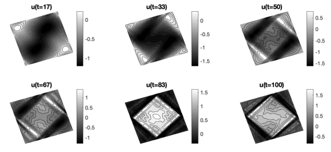
Figure 1. Contour plots of a numerical solution to (1.1) for $\Omega$ given by a unit square tilted by $\pi/10$ (see §2.5), with $f(x)=e^{-5\pi^{2}(x-x^{0})^{2}}$, where $x^{0}$ is the center and $\lambda=0.8$. In that case the rotation number of the billiard ball map is $\frac{1}{2}$ (see Figure 9) and the classical attractor is given by a parallelogram on which $u$ develops a singularity – see Theorem 1.

They can be described by linear perturbations of the initial state of rest of a stable-stratified fluid (dense fluid lies everywhere below less-dense fluid and the isodensity surfaces are all horizontal). Forcing can take place at linear level by pushing fluid away from this equilibrium state either mechanically, by wind, a piston, a moving boundary, or thermodynamically, by spatially differential heating or evaporation/rain.

The mechanism behind formation of internal waves comes from ray dynamics of the classical system which underlies wave equations – see §1.1 for the case of nonlinear ray dynamics relevant to the case we consider. When parameters of the system produce hyperbolic dynamics, attractors are observed in wave evolution – see Figure 1. This phenomenon is both physically and theoretically more accessible in dimension two. The analysis in the physics literature, see [22], [35], has focused on constructions of standing and propagating waves and did not address the evolution problem analytically. (See however [2] for an analysis of a numerical approach to the evolution problem.) In this paper we prove the emergence of singular profiles in the long time evolution of linear waves for two dimensional domains.

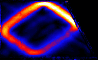
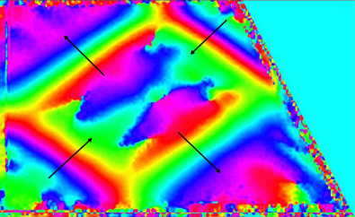
Figure 2. Experimental results of Hazewinkel et al [17]: horizontal component of the observed perturbation buoyancy gradient projected onto a field that oscillates at the forcing frequency, thus reducing the time series to an amplitude field (left) and a phase field (right). In terms of our Theorem 1 this corresponds to amplitude and phase of $u^{+}$. The arrows indicate directions of phase propagation in agreement with our analysis, shown on Figure 4.

The model we consider is described as follows. Let $\Omega\subset\mathbb{R}^{2}=\{x=(x_{1},x_{2}):x_{j}\in\mathbb{R}\}$ be a bounded simply connected open set with $C^{\infty}$ boundary $\partial\Omega$. Following the fluid mechanics literature we consider the following evolution problem, sometimes referred to as the Poincaré problem:

$$(\partial_{t}^{2}\Delta+\partial_{x_{2}}^{2})u=f(x)\cos\lambda t,\ \ u|_{t=0}=\partial_{t}u|_{t=0}=0,\ \ u|_{\partial\Omega}=0,$$ (1.1)

where $\lambda\in(0,1)$ and $\Delta:=\partial_{x_{1}}^{2}+\partial_{x_{2}}^{2}$, see Sobolev [32, equation (48)], Ralston [28, p.374], Maas et al [23], Brouzet [4, §§1.1.2–3], Dauxois et al [8], Colin de Verdière–Saint-Raymond [6], Sibgatullin–Ermanyuk [31], and references given there. It models internal waves in a stratified fluid in an effectively two-dimensional aquarium $\Omega$ with an oscillatory forcing term (here we follow [6] rather than change the boundary condition). The geometry of $\Omega$ and the forcing frequency $\lambda$ can produce concentration of the fluid velocity $\mathbf{v}=(\partial_{x_{2}}u,-\partial_{x_{1}}u)$ on attractors. This phenomenon was predicted by Maas–Lam [24] and was then observed experimentally by Maas–Benielli–Sommeria–Lam [23], see Figure 2 for experimental data from the more recent [17]. (See also the earlier work of Wunsch [40] which studied the case of an internal wave converging to a corner, along a trajectory of the type pictured on Figure 7.) In this paper we provide a mathematical explanation: as mentioned above the physics papers concentrated on the analysis of modes and classical dynamics rather than on the long time behaviour of solutions to (1.1).

1.1. Assumptions on $\Omega$ and $\lambda$

The assumptions on $\Omega$ and $\lambda$ which guarantee existence of singular profiles (internal waves) in long time evolution of (1.1) are formulated using a “chess billiard” – see [27], [21] for recent studies and references. It was first considered in similar context by John [20] (see also the later work of Aleksandrjan [1]) and was the basis of the analysis in [24]. It is defined as the reflected bicharacteristic flow for $(1-\lambda^{2})\xi_{2}^{2}-\lambda^{2}\xi_{1}^{2}$, which is the Hamiltonian for the $1+1$ wave equation with $x_{2}$ corresponding to time and the speed given by $c=\lambda/\sqrt{1-\lambda^{2}}$ – see Figure 3 and §2.1. This flow has a simple reduction to the boundary which we describe using a factorization of the quadratic form dual to $(1-\lambda^{2})\xi_{2}^{2}-\lambda^{2}\xi_{1}^{2}$:

$$-\frac{x_{1}^{2}}{\lambda^{2}}+\frac{x_{2}^{2}}{1-\lambda^{2}}=\ell^{+}(x,\lambda)\ell^{-}(x,\lambda),\quad\ell^{\pm}(x,\lambda):=\pm{x_{1}\over\lambda}+{x_{2}\over\sqrt{1-\lambda^{2}}}.$$ (1.2)

We often suppress the dependence on $\lambda$, writing simply $\ell^{\pm}(x)$. Same applies to other $\lambda$-dependent objects introduced below.

Definition 1.

Let $0<\lambda<1$. We say that $\Omega$ is $\lambda$-simple if each of the functions $\partial\Omega\ni x\mapsto\ell^{\pm}(x,\lambda)$ has only two critical points, which are both nondegenerate. We denote these minimum/maximum points by $x^{\pm}_{\min}(\lambda),x^{\pm}_{\max}(\lambda)$.

Under the assumption of $\lambda$-simplicity we define the following two smooth orientation reversing involutions on the boundary (see §2.1 for more details):

$$\gamma^{\pm}(\bullet,\lambda):\partial\Omega\to\partial\Omega,\quad\ell^{\pm}(x)=\ell^{\pm}(\gamma^{\pm}(x)).$$ (1.3)

These maps correspond to interchanging intersections of the boundary with lines with slopes $\mp 1/c$, respectively – see Figure 3. The chess billiard map $b(\bullet,\lambda)$ is defined as the composition

$$b:=\gamma^{+}\circ\gamma^{-}$$ (1.4)

and is a $C^{\infty}$ orientation preserving diffeomorphism of $\partial\Omega$.

Figure 3. Left: the involutions $\gamma^{\pm}$ and the chess billiard map $b$. Right: a forward trajectory of the map $b$ on a trapezium with rounded corners, converging to a periodic trajectory. We remark that the effect of smoothed corner on classical dynamics was investigated by Manders–Duistermaat–Maas [25], see also §2.4.

Denoting by $b^{n}$ the $n$-th iterate of $b$, we consider the set of periodic points

$$\Sigma_{\lambda}:=\{x\in\partial\Omega\mid b^{n}(x,\lambda)=x\text{ for some }n\geq 1\}.$$ (1.5)

If $\Sigma_{\lambda}\neq\emptyset$, then all the periodic points in $\Sigma_{\lambda}$ have the same minimal period, see §2.1.

We are now ready to state the dynamical assumptions on the chess billiard:

Definition 2.

Let $0<\lambda<1$. We say that $\lambda$ satisfies the Morse–Smale conditions if:

1. $\Omega$ is $\lambda$-simple;

2. the map $b$ has periodic points, that is $\Sigma_{\lambda}\neq\emptyset$;

3. the periodic points are hyperbolic, that is $\partial_{x}b^{n}(x,\lambda)\neq 1$ for all $x\in\Sigma_{\lambda}$ where $n$ is the minimal period.

Under the Morse–Smale conditions we have $\Sigma_{\lambda}=\Sigma_{\lambda}^{+}\sqcup\Sigma_{\lambda}^{-}$ where $\Sigma_{\lambda}^{+},\Sigma_{\lambda}^{-}$ are the sets of attractive, respectively repulsive, periodic points of $b$:

$$\Sigma_{\lambda}^{+}:=\{x\in\Sigma_{\lambda}\mid\partial_{x}b^{n}(x,\lambda)<1\},\quad\Sigma_{\lambda}^{-}:=\{x\in\Sigma_{\lambda}\mid\partial_{x}b^{n}(x,\lambda)>1\}.$$ (1.6)

Moreover, each of the involutions $\gamma^{\pm}$ exchanges $\Sigma^{+}_{\lambda}$ with $\Sigma^{-}_{\lambda}$, see (2.2).

For $y\in\partial\Omega$, let

$$\Gamma_{\lambda}^{\pm}(y):=\{x\in\Omega\mid\ell^{\pm}(x,\lambda)=\ell^{\pm}(y,\lambda)\}$$ (1.7)

be the open line segment connecting $y$ with $\gamma^{\pm}(y,\lambda)$. Denote $\Gamma_{\lambda}(y):=\Gamma_{\lambda}^{+}(y)\cup\Gamma_{\lambda}^{-}(y)$. Then $\Gamma_{\lambda}(\Sigma_{\lambda})$ gives the closed trajectories of the chess billiard inside $\Omega$.

Figure 4. A visualization of the Lagrangian submanifolds (1.9) corresponding to attractive and repulsive cycles of $b$ given in (1.4). The parallelogram represents the projection of the attractive ($+$) and repulsive ($-$) Lagrangians $\Lambda^{\pm}(\lambda)$ and the arrows perpendicular to the sides represent the conormal directions distinguishing the two Lagrangians. We also indicate the corresponding sets on the boundary: $\Sigma_{\lambda}^{\pm}$ are the attractive ($+$) and repulsive ($-$) periodic points of $b$ given by (1.4) and the arrows indicate the sign of the conormal directions.

For $y\in\partial\Omega$ which is not a critical point of $\ell^{+}$, we split the conormal bundle $N^{*}\Gamma_{\lambda}^{+}(y)$ into the positive/negative directions:

$$\begin{gathered}N^{*}\Gamma_{\lambda}^{+}(y)\setminus 0=N^{*}_{+}\Gamma_{\lambda}^{+}(y)\sqcup N^{*}_{-}\Gamma_{\lambda}^{+}(y),\\ N^{*}_{\pm}\Gamma_{\lambda}^{+}(y):=\{(x,\tau d\ell^{+}(x))\mid x\in\Gamma_{\lambda}^{+}(y),\ \pm(\partial_{\theta}\ell^{+}(y))\tau>0\}\end{gathered}$$ (1.8)

and similarly for $N^{*}\Gamma_{\lambda}^{-}(y)$. Here $\partial_{\theta}$ is the derivative with respect to a positively oriented (that is, counterclockwise when $\Omega$ is convex) parametrization of the boundary $\partial\Omega$. Note that the orientation depends on the choice of $y$ and not just on $\Gamma_{\lambda}^{\pm}(y)$: we have $N^{*}_{+}\Gamma_{\lambda}^{\pm}(\gamma^{\pm}(y))=N^{*}_{-}\Gamma_{\lambda}^{\pm}(y)$.

We now define Lagrangian submanifolds $\Lambda^{\pm}(\lambda)\subset T^{*}\Omega\setminus 0$ by

$$\Lambda^{\pm}(\lambda):=N_{+}^{*}\Gamma^{-}_{\lambda}(\Sigma^{\pm}_{\lambda})\sqcup N_{-}^{*}\Gamma^{+}_{\lambda}(\Sigma^{\mp}_{\lambda}),$$ (1.9)

see Figure 4. We note that $\pi(\Lambda^{\pm}(\lambda))=\Gamma_{\lambda}(\Sigma_{\lambda})$ and $N_{-}^{*}\Gamma^{\pm}_{\lambda}(\Sigma^{+}_{\lambda})=N_{+}^{*}\Gamma^{\pm}_{\lambda}(\Sigma^{-}_{\lambda})$.

1.2. Statement of results

The main result of this paper is formulated using the concept of wave front set, see [18, §8.1] and [19, Theorem 18.1.27]. The wave front set of a distribution, $\operatorname{WF}(u)$, is a closed subspace of the cotangent bundle of $T^{*}\Omega\setminus 0$ and it provides phase space information about singularities. Its projection to the base, $\pi(\operatorname{WF}(u))$, is the singular support, $\operatorname{sing}\operatorname{supp}u$.

Theorem 1.

Suppose that $\Omega$ and $\lambda\in(0,1)$ satisfy the Morse–Smale conditions of Definition 2. Assume that $f\in C^{\infty}_{\mathrm{c}}(\Omega;\mathbb{R})$. Then the solution to (1.1) is decomposed as

$$\begin{gathered}u(t)=\operatorname{Re}\big{(}e^{i\lambda t}u^{+}\big{)}+r(t)+e(t),\quad u^{+}\in H^{\frac{1}{2}-}(\Omega),\quad\operatorname{WF}(u^{+})\subset\Lambda^{+}(\lambda),\\ r(t)\in H^{1}(\Omega),\quad\|r(t)\|_{H^{1}(\Omega)}\leq C,\quad\|e(t)\|_{H^{\frac{1}{2}-}(\Omega)}\to 0\quad\text{as }t\to\infty,\end{gathered}$$ (1.10)

where $\Lambda^{+}(\lambda)\subset T^{*}\Omega\setminus 0$ is the attracting Lagrangian – see (1.9) and Figure 4. In particular, $\operatorname{sing}\operatorname{supp}u^{+}$ is contained in the union of closed orbits of the chess billiard flow. In addition, $u^{+}$ is a Lagrangian distribution, $u^{+}\in I^{-1}(\overline{\Omega},\Lambda^{+}(\lambda))$ (see §3.2) and $u^{+}|_{\partial\Omega}=0$ (well defined because of the wave front set condition).

For a numerical illustration of (1.10), see Figure 1. We remark that numerically it is easier to consider polygonal domains – see §2.4 for a discussion of the stability of our assumptions for smoothed out polygonal domains.

Theorem 1 is proved using spectral properties of a self-adjoint operator associated to the evolution equation (1.1). To define it, let $\Delta_{\Omega}$ be the (negative definite) Dirichlet Laplacian of $\Omega$ with the inverse denoted by $\Delta_{\Omega}^{-1}:H^{-1}(\Omega)\to H_{0}^{1}(\Omega)$. Then

$$P:=\partial_{x_{2}}^{2}\Delta_{\Omega}^{-1}:H^{-1}(\Omega)\to H^{-1}(\Omega),\ \ \ \langle u,w\rangle_{H^{-1}(\Omega)}:=\langle\nabla\Delta_{\Omega}^{-1}u,\nabla\Delta_{\Omega}^{-1}w\rangle_{L^{2}(\Omega)},$$ (1.11)

is a bounded non-negative (hence self-adjoint) operator studied by Aleksandrjan [1] and Ralston [28] – see §7.1. Studying the spectrum of $P$ is referred to as a Poincaré problem.

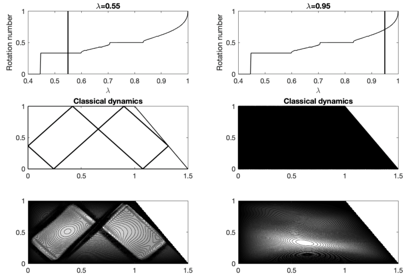
Figure 5. Numerical illustration of Theorem 2: contour plots of $|u(x)|$ for $u=(\partial_{x_{2}}^{2}-(\lambda^{2}+i\varepsilon)\Delta_{\Omega})^{-1}f$ where $\varepsilon=0.005$ and $f(x)=e^{-10(x-(\frac{1}{2},\frac{1}{2}))^{2}}$ and $\Omega=\mathcal{T}_{0.5}$ (see §2.5). On the left, the rotation number is given by $\frac{1}{3}$ and we see concentration on an attractor; on the right, the rotation number is (nearly) irrational and, as $\varepsilon\to 0+$, $u$ is expected to be uniformly distributed [22]. Morse–Smale assumptions do not hold, at least not on scales relevant to numerical calculations and trajectories are uniformly distributed in the trapezium. In the contour plots of $|u(x)|$ black corresponds to $0$.

The evolution equation (1.1) is equivalent to

$$(\partial^{2}_{t}+P)w=f\cos\lambda t,\ \ \ w|_{t=0}=\partial_{t}w|_{t=0}=0,\ \ f\in C^{\infty}_{\rm{c}}(\Omega;\mathbb{R}),\ \ \ u=\Delta_{\Omega}^{-1}w.$$ (1.12)

This equation is easily solved using the functional calculus of $P$:

$$\begin{gathered}w(t)=\operatorname{Re}\big{(}e^{i\lambda t}\mathbf{W}_{t,\lambda}(P)f\big{)}\qquad\text{where}\\ \mathbf{W}_{t,\lambda}(z)=\int_{0}^{t}{\sin\big{(}s\sqrt{z}\big{)}\over\sqrt{z}}e^{-i\lambda s}\,ds=\sum_{\pm}{1-e^{-it(\lambda\pm\sqrt{z})}\over 2\sqrt{z}(\sqrt{z}\pm\lambda)}.\end{gathered}$$ (1.13)

Using the Fourier transform of the Heaviside function (see (3.26)), we see that for any $\varphi\in C^{\infty}_{\mathrm{c}}(\mathbb{R})$ we have

$$\int_{\mathbb{R}}{1-e^{-it\zeta}\over\zeta}\varphi(\zeta)\,d\zeta=i\int_{0}^{t}\widehat{\varphi}(\eta)\,d\eta\ \xrightarrow{t\to\infty}\ i\int_{0}^{\infty}\widehat{\varphi}(\eta)\,d\eta=\int_{\mathbb{R}}(\zeta-i0)^{-1}\varphi(\zeta)\,d\zeta$$

and thus for any $\lambda\in(0,1)$ we have the distributional limit

$$\mathbf{W}_{t,\lambda}(z)\to(z-\lambda^{2}+i0)^{-1}\quad\text{as }t\to\infty\quad\text{in }\mathcal{D}^{\prime}_{z}((0,\infty)).$$ (1.14)

This suggests that, as long as we only look at the spectrum of $P$ near $\lambda^{2}$ (the rest of the spectrum contributing the term $r(t)$ in Theorem 1), if the spectral measure of $P$ applied to $f$ is smooth in the spectral parameter $z$, then $\mathbf{W}_{t,\lambda}(P)f\to(P-\lambda^{2}+i0)^{-1}f$ as $t\to\infty$. By Stone’s Formula, it suffices to establish the limiting absorption principle for the operator $P$ near $\lambda^{2}$ and that is the content of

Theorem 2.

Suppose that $\mathcal{J}\subset(0,1)$ is an open interval such that each $\lambda\in\mathcal{J}$ satisfies the Morse–Smale conditions of Definition 2. Then for each $f\in C^{\infty}_{\mathrm{c}}(\Omega)$ and $\lambda\in\mathcal{J}$ the limits

$$(P-\lambda^{2}\pm i0)^{-1}f=\lim_{\varepsilon\to 0+}(P-(\lambda\mp i\varepsilon)^{2})^{-1}f\quad\text{in }\mathcal{D}^{\prime}(\Omega)$$ (1.15)

exist and the spectrum of $P$ is purely absolutely continuous in $\mathcal{J}^{2}:=\{\lambda^{2}\mid\lambda\in\mathcal{J}\}$:

$$\sigma(P)\cap\mathcal{J}^{2}=\sigma_{\rm{ac}}(P)\cap\mathcal{J}^{2}.$$ (1.16)

Moreover,

$$(P-\lambda^{2}\pm i0)^{-1}f\in I^{1}(\overline{\Omega},\Lambda^{\pm}(\lambda))\ \subset\ H^{-\frac{3}{2}-}(\Omega),$$ (1.17)

where $\Lambda^{\pm}(\lambda)$ are given in (1.9) and the definition of the conormal spaces $I^{1}(\overline{\Omega},\Lambda^{\pm}(\lambda))$ is reviewed in §3.2.

Remarks. 1. The proof provides a more precise statement based on a reduction to the boundary – see §7. We also have smooth dependence on $\lambda$ which plays a crucial role in proving Theorem 1 as in [13, §5] – see §8. This precise information is important in obtaining the $H^{\frac{1}{2}-}$ remainder in (1.10). The singular profile in Theorem 1 satisfies

$$u^{+}=\Delta_{\Omega}^{-1}(P-\lambda^{2}+i0)^{-1}f,$$

which agrees with the heuristic argument following (1.14).

2. As noted in [28], $\sigma(P)=[0,1]$ but as emphasized there and in numerous physics papers the structure of the spectrum of $P$ is far from clear. Here we only characterize the spectrum (1.16) under the Morse–Smale assumptions of Definition 2.

Rather than working with $P$, we consider the closely related stationary Poincaré problem

$$(\partial_{x_{2}}^{2}-\omega^{2}\Delta)u_{\omega}=f\in C_{\rm c}^{\infty},\quad u_{\omega}|_{\partial\Omega}=0,\quad\operatorname{Re}\omega\in(0,1),\quad\operatorname{Im}\omega>0.$$

Then $u_{\lambda+i\varepsilon}\in C^{\infty}(\overline{\Omega})$ has a limit in $\mathcal{D}^{\prime}(\Omega)$ which satisfies $u_{\lambda+i0}\in I^{-1}(\overline{\Omega},\Lambda^{-}(\lambda))$, and we have $(P-\lambda^{2}-i0)^{-1}f=\Delta u_{\lambda+i0}$.

1.3. Related mathematical work

Motivated by the study of internal waves results similar to Theorems 1 and 2 were obtained for self-adjoint 0th order pseudodifferential operators on 2D tori with dynamical conditions in Definitions 1 and 2 replaced by demanding that a naturally defined flow is Morse–Smale. That was done first by Colin de Verdière–Saint Raymond [6, 5], with different proofs provided by Dyatlov–Zworski [13]. The question of modes of viscosity limits in such models (addressing physics questions formulated for domains with boundary – see Rieutord–Valdettaro [29] and references given there) were investigated by Galkowski–Zworski [15] and Wang [38]. Finer questions related to spectral theory were also answered in [39]. Unlike in the situation considered in this paper, embedded eigenvalues are possible in the case of 0th order pseudodifferential operators [34].

The dynamical system (1.4) was recently studied by Nogueira–Troubetzkoy [27] and by Lenci et al [21]. We refer to those papers for additional references and dynamical results.

1.4. Organization of the paper

In §2 we provide a self-contained analysis of the dynamical system given by the diffeomorphism (1.4). We emphasize properties needed in the analysis of the operator (1.11): properties of pushforwards by $\ell^{\pm}$ and existence of suitable escape/Lyapounov functions. §3 is devoted to a review of microlocal analysis used in this paper and in particular to definitions and properties of conormal/Lagrangian spaces used in the formulations of Theorems 1 and 2. In §4 we describe reduction to the boundary using 1+1 Feynman propagators which arise naturally in the limiting absorption principles. Despite the presence of characteristic points, the restricted operator enjoys good microlocal properties – see Proposition 4.15. Microlocal analysis of that operator is given in §5 with the key estimate (5.19) motivated by Lasota–Yorke inequalities and radial estimates. The self-contained §6 analyses wave front set properties of distributions invariant under the diffeomorphisms (1.4). These results are combined in §7 to give the proof of the limiting absorption principle of Theorem 2. Finally, in §8 we follow the strategy of [13] to describe long time properties of solutions to (1.1) – see Theorem 1.

2. Geometry and dynamics

In this section we assume that $\Omega\subset\mathbb{R}^{2}$ is an open bounded simply connected set with $C^{\infty}$ boundary $\partial\Omega$ and review the basic properties of the involutions $\gamma^{\pm}$ and the chess billiard $b$ defined in (1.3), (1.4). We orient $\partial\Omega$ in the positive direction as the boundary of $\Omega$ (that is, counterclockwise if $\Omega$ is convex).

2.1. Basic properties

Fix $\lambda\in(0,1)$ such that $\Omega$ is $\lambda$-simple in the sense of Definition 1. We first show that the involutions $\gamma^{\pm}$ defined in (1.3) are smooth. Away from the critical set $\{x^{\pm}_{\min},x^{\pm}_{\max}\}$ this is immediate. Next, we write

$$\ell^{\pm}(x) =\ell^{\pm}(x^{\pm}_{\min})+\theta^{\pm}_{\min}(x)^{2}\quad\text{for $x$ near $x^{\pm}_{\min}$},$$ (2.1)

$$\ell^{\pm}(x) =\ell^{\pm}(x^{\pm}_{\max})-\theta^{\pm}_{\max}(x)^{2}\quad\text{for $x$ near $x^{\pm}_{\max}$}$$

where $\theta^{\pm}_{\min},\theta^{\pm}_{\max}$ are local coordinate functions on $\partial\Omega$ which map $x^{\pm}_{\min},x^{\pm}_{\max}$ to 0. Then for $x$ near $x^{\pm}_{\min}$ the point $\gamma^{\pm}(x)$ satisfies the equation

$$\theta^{\pm}_{\min}(\gamma^{\pm}(x))=-\theta^{\pm}_{\min}(x)$$

and similarly near $x^{\pm}_{\max}$. This shows the smoothness of $\partial\Omega\ni x\mapsto\gamma^{\pm}(x)$ near the critical points.

Next, note that since $\gamma^{\pm}$ are involutions, $b$ is conjugate to its inverse:

$$b^{-1}=\gamma^{\pm}\circ b\circ\gamma^{\pm}.$$ (2.2)

Therefore $\Sigma_{\lambda}^{+}=\gamma^{\pm}(\Sigma_{\lambda}^{-})$ where $\Sigma_{\lambda}^{\pm}$ are defined in (1.6). Since $x^{\pm}_{\min},x^{\pm}_{\max}$ are fixed points of $\gamma^{\pm}$, the Morse–Smale conditions (see Definition 2) implies that there are no characteristic periodic points:

$$\Sigma_{\lambda}\cap\mathscr{C}_{\lambda}=\emptyset\quad\text{where}\quad\mathscr{C}_{\lambda}:=\mathscr{C}_{\lambda}^{+}\sqcup\mathscr{C}_{\lambda}^{-},\quad\mathscr{C}_{\lambda}^{\pm}:=\{x^{\pm}_{\min}(\lambda),x^{\pm}_{\max}(\lambda)\}.$$ (2.3)

2.1.1. Useful identities

For $x\in\partial\Omega$ and $\lambda\in(0,1)$ we define the signs

$$\nu^{\pm}(x,\lambda):=\operatorname{sgn}\partial_{\theta}\ell^{\pm}(x,\lambda)$$ (2.4)

where $\partial_{\theta}$ is the derivative along $\partial\Omega$ with respect to a positively oriented parametrization.

Lemma 2.1.

Assume that $\Omega$ is $\lambda$-simple. Then for all $x\in\partial\Omega$

$$\operatorname{sgn}\ell^{\mp}(\gamma^{\pm}(x)-x)=\pm\nu^{\pm}(x),$$ (2.5)

$$\nu^{\pm}(\gamma^{\pm}(x))=-\nu^{\pm}(x),$$ (2.6)

$$\partial_{\lambda}\ell^{\pm}(x,\lambda)={2\lambda^{2}-1\over 2\lambda(1-\lambda^{2})}\ell^{\pm}(x,\lambda)+{1\over 2\lambda(1-\lambda^{2})}\ell^{\mp}(x,\lambda).$$ (2.7)

Proof.

To see (2.5), we first notice that it holds when $x\in\{x^{\pm}_{\min},x^{\pm}_{\max}\}$, as then both sides are equal to 0. Now, assume that $\gamma^{\pm}(x)\neq x$ (that is, $x\notin\{x^{\pm}_{\min},x^{\pm}_{\max}\}$). Denote by $v(x)\in\mathbb{R}^{2}$ the velocity vector of the parametrization at the point $x\in\partial\Omega$. The vector $\gamma^{\pm}(x)-x\in\mathbb{R}^{2}$ is pointing into $\Omega$ at the point $x\in\partial\Omega$. Since we use a positively oriented parametrization, the vectors $v(x),\gamma^{\pm}(x)-x$ form a positively oriented basis. We now note that $\ell^{+},\ell^{-}$ form a positively oriented basis of the dual space to $\mathbb{R}^{2}$, and hence

$$\det\begin{pmatrix}\ell^{+}(v(x))&\ell^{+}(\gamma^{\pm}(x)-x)\\ \ell^{-}(v(x))&\ell^{-}(\gamma^{\pm}(x)-x)\end{pmatrix}>0.$$

Since $\partial_{\theta}\mathcal{\ell}^{\pm}(x)=\ell^{\pm}(v(x))$, this gives (2.5). The identity (2.6) follows from (2.5), and (2.7) is verified by a direct computation. ∎

The next statement is used in the proof of Lemma 4.9.

Lemma 2.2.

Assume that $\Omega$ is $\lambda$-simple. Then for all $y\in\partial\Omega$ and $x\in\Omega$

$$\nu^{+}(y)\ell^{-}(x-y)>0\quad\text{or}\quad\nu^{-}(y)\ell^{+}(x-y)<0\quad\text{(or both).}$$ (2.8)

Proof.

Let $\Gamma^{\pm}_{\lambda}(y)$ be the sets defined in (1.7) and recall that they are open line segments with endpoints $y,\gamma^{\pm}(y)$. Then by (2.5),

$$\Omega\cap R^{\pm}(y)=\emptyset\quad\text{where}\quad R^{\pm}(y):=\{x\in\mathbb{R}^{2}\mid\ell^{\pm}(x-y)=0,\ \pm\nu^{\pm}(y)\ell^{\mp}(x-y)\leq 0\}.$$

The sets $R^{\pm}(y)$ are closed rays starting at $y$ when $\nu^{\pm}(y)\neq 0$ and lines passing through $y$ when $\nu^{\pm}(y)=0$. Any continuous curve starting at the set of $x\in\mathbb{R}^{2}$ satisfying (2.8) and ending in the complement of this set has to intersect $R^{+}(y)\cup R^{-}(y)$, as can be seen (in the case $\nu^{\pm}(y)\neq 0$) by applying the Intermediate Value Theorem to the pullback to that curve of the function $x\mapsto\max(\nu^{+}(y)\ell^{-}(x-y),-\nu^{-}(y)\ell^{+}(x-y))$. Thus, since $\Omega$ is connected and contains at least one point $x$ satisfying (2.8) (for instance, take any point in $\Gamma^{\pm}_{\lambda}(y)$), all points $x\in\Omega$ satisfy (2.8). ∎

2.1.2. Properties of pushforwards

We next show basic properties of pushforwards of smooth functions by the maps $\partial\Omega\ni x\mapsto\ell^{\pm}(x,\lambda)$, which are used in the proof of Lemma 4.8. Fix $\lambda\in(0,1)$ such that $\Omega$ is $\lambda$-simple and define

$$\ell^{\pm}_{\min}:=\ell^{\pm}(x^{\pm}_{\min}),\quad\ell^{\pm}_{\max}:=\ell^{\pm}(x^{\pm}_{\max}),$$ (2.9)

so that $\ell^{\pm}$ maps $\partial\Omega$ onto the interval $[\ell^{\pm}_{\min},\ell^{\pm}_{\max}]$. We again fix a positively oriented coordinate $\theta$ on $\partial\Omega$.

Lemma 2.3.

1. Assume that $f\in C^{\infty}(\partial\Omega)$ and define $\Pi^{\pm}_{\lambda}f\in\mathcal{E}^{\prime}(\mathbb{R})$ by the formula

$$\int_{\mathbb{R}}\Pi_{\lambda}^{\pm}f(s)\varphi(s)\,ds=\int_{\partial\Omega}f(x)\varphi(\ell^{\pm}(x))\,d\theta(x)\quad\text{for all}\quad\varphi\in C^{\infty}(\mathbb{R}).$$ (2.10)

Then $\operatorname{supp}\Pi_{\lambda}^{\pm}f\subset[\ell^{\pm}_{\min},\ell^{\pm}_{\max}]$ and

$$\sqrt{(s-\ell^{\pm}_{\min})(\ell^{\pm}_{\max}-s)}\,\Pi_{\lambda}^{\pm}f(s)\ \in\ C^{\infty}([\ell^{\pm}_{\min},\ell^{\pm}_{\max}]).$$ (2.11)

2. Assume that $f\in C^{\infty}(\partial\Omega)$ and define the functions $\Upsilon^{\pm}_{\lambda}f$ on $(\ell^{\pm}_{\min},\ell^{\pm}_{\max})$ by

$$\Upsilon^{\pm}_{\lambda}f(s):=\sum_{x\in\partial\Omega,\,\ell^{\pm}(x)=s}f(x),\quad s\in(\ell^{\pm}_{\min},\ell^{\pm}_{\max}).$$

Then $\Upsilon^{\pm}_{\lambda}f\in C^{\infty}([\ell^{\pm}_{\min},\ell^{\pm}_{\max}])$.

Proof.

1. The support property follows immediately from the definition: if $\operatorname{supp}\varphi\cap[\ell^{\pm}_{\min},\ell^{\pm}_{\max}]=\emptyset$, then $\varphi\circ\ell^{\pm}=0$ on $\partial\Omega$ and thus $\int(\Pi_{\lambda}^{\pm}f)\varphi=0$.

To show (2.11), we compute

$$\Pi_{\lambda}^{\pm}f(s)=\sum_{x\in\partial\Omega,\,\ell^{\pm}(x)=s}{f(x)\over|\partial_{\theta}\ell^{\pm}(x)|}\quad\text{for all}\quad s\in(\ell^{\pm}_{\min},\ell^{\pm}_{\max}).$$ (2.12)

It follows that $\Pi_{\lambda}^{\pm}f$ is smooth on the open interval $(\ell^{\pm}_{\min},\ell^{\pm}_{\max})$. Next, note that (2.11) does not depend on the choice of the parametrization $\theta$ since changing the parametrization amounts to multiplying $f$ by a smooth positive function. Thus we can use the local coordinate $\theta=\theta^{\pm}_{\min}$ near $x^{\pm}_{\min}$ introduced in (2.1). With this choice we have $\ell^{\pm}(x)=\ell^{\pm}_{\min}+\theta^{2}$ and the formula (2.12) gives for $s$ near $\ell^{\pm}_{\min}$

$$\Pi_{\lambda}^{\pm}f(s)={f(\sqrt{s-\ell^{\pm}_{\min}})+f(-\sqrt{s-\ell^{\pm}_{\min}})\over 2\sqrt{s-\ell^{\pm}_{\min}}}$$

where we view $f$ as a function of $\theta$. It follows that $\sqrt{s-\ell^{\pm}_{\min}}\,\Pi_{\lambda}^{\pm}f(s)$ is smooth at the left endpoint of the interval $(\ell^{\pm}_{\min},\ell^{\pm}_{\max})$. Similar analysis shows that $\sqrt{\ell^{\pm}_{\max}-s}\,\Pi_{\lambda}^{\pm}f(s)$ is smooth at the right endpoint of this interval.

2. This is proved similarly to part 1, where we no longer have $|\partial_{\theta}\ell^{\pm}(x)|$ in the denominator in (2.12).∎

2.1.3. Dynamics of the chess billiard

We now give a description of the dynamics of the orientation preserving diffeomorphism $b=\gamma^{+}\circ\gamma^{-}$ in the presense of periodic points.

Lemma 2.4.

Assume that $\Sigma_{\lambda}\neq\emptyset$ (see (1.5)). Then:

1. all periodic points of $b$ have the same minimal period;

2. for each $x\in\partial\Omega$, the trajectory $b^{k}(x)$ converges to $\Sigma_{\lambda}$ as $k\to\pm\infty$;

3. if $\partial_{x}b^{n}\neq 1$ on $\Sigma_{\lambda}$ where $n$ denotes the minimal period, then the set $\Sigma_{\lambda}$ is finite.

Proof.

See for example [10, §1.1] or [37] for the proof of the first two claims. The last claim follows from the fact that $\Sigma_{\lambda}$ is the set of solutions to $b^{n}(x)=x$ and thus $\partial_{x}b^{n}(x)\neq 0$ implies that it consists of isolated points. ∎

We finally discuss the rotation number of $b$. Fix a positively oriented parametrization on $\partial\Omega$ which identifies it with the circle $\mathbb{S}^{1}=\mathbb{R}/\mathbb{Z}$ and denote by $\pi:\mathbb{R}\to\partial\Omega$ the covering map. Consider a lift of $b(\bullet,\lambda)$ to $\mathbb{R}$, that is, an orientation preserving diffeomorphism $\mathbf{b}(\bullet,\lambda):\mathbb{R}\to\mathbb{R}$ such that

$$\pi(\mathbf{b}(\theta,\lambda))=b(\pi(\theta),\lambda)\quad\text{for all}\quad\theta\in\mathbb{R}.$$

Denote by $\mathbf{b}^{k}(\bullet,\lambda)$ the $k$-th iterate of $\mathbf{b}(\bullet,\lambda)$. Define the rotation number of $b(\bullet,\lambda)$ as

$$\mathbf{r}(\lambda):=\lim_{k\to\infty}{\mathbf{b}^{k}(\theta,\lambda)-\theta\over k}\mod\mathbb{Z}\ \in\ \mathbb{R}/\mathbb{Z}.$$ (2.13)

The limit exists and is independent of the choice of $\theta\in\mathbb{R}$ and of the lift $\mathbf{b}$. We refer to [37] for a proof of this fact as well that of the following

Lemma 2.5.

The rotation number $\mathbf{r}(\lambda)$ is rational if and only if $\Sigma_{\lambda}\neq\emptyset$. In this case $\mathbf{r}(\lambda)={q\over n}\bmod\mathbb{Z}$ where $n>0$ is the minimal period of the periodic points and $q\in\mathbb{Z}$ is coprime with $n$.

We remark that $b(\bullet,\lambda)$ cannot have fixed points: indeed, if $x\in\partial\Omega$ and $b(x)=x$, then $\gamma^{+}(x)=\gamma^{-}(x)$ which is impossible. We then fix the lift $\mathbf{b}$ for which

$$0<\mathbf{b}(0,\lambda)<1.$$ (2.14)

With this choice we have $0<\mathbf{b}^{k}(0,\lambda)<k$ for all $k\geq 0$ and thus (2.13) defines the rotation number $\mathbf{r}(\lambda)$ which satisfies $0<\mathbf{r}(\lambda)<1$.

2.2. Dependence on $\lambda$

We now discuss the dependence of the dynamics of the chess billiard map $b(\bullet,\lambda)$ on $\lambda$. We first give a stability result:

Lemma 2.6.

The set of $\lambda\in(0,1)$ satisfying the Morse–Smale conditions (see Definition 2) is open. Moreover, the maps $\gamma^{\pm}(x,\lambda)$ and $b(x,\lambda)$, as well as the sets $\Sigma_{\lambda}$, depend smoothly on $\lambda$ as long as $\lambda$ satisfies the Morse–Smale conditions.

Proof.

Assume that $\lambda_{0}$ satisfies the Morse–Smale conditions. We need to show that all $\lambda$ close enough to $\lambda_{0}$ satisfy this condition as well. From (1.2) we see that the functions $\ell^{\pm}(x,\lambda)$ depend smoothly on $x\in\partial\Omega,\lambda\in(0,1)$. Therefore, $\Omega$ is $\lambda$-simple for $\lambda$ close to $\lambda_{0}$. Moreover, $\gamma^{\pm}(x,\lambda)$ and $b(x,\lambda)$ depend smoothly on $\lambda$ as long as $\Omega$ is $\lambda$-simple.

Next, let $m>0$ be the number of points in $\Sigma_{\lambda_{0}}$ and let $n$ be their minimal period under $b(\bullet,\lambda_{0})$. Since $\partial_{x}b^{n}(x,\lambda_{0})\neq 1$ on $\Sigma_{\lambda_{0}}$, by the Implicit Function Theorem for $\lambda$ close to $\lambda_{0}$ the equation $b^{n}(x,\lambda)=x$ has exactly $m$ solutions, which depend smoothly on $\lambda$. It follows that $\lambda$ satisfies the Morse–Smale conditions. ∎

Lemmas 2.5 and 2.6 imply in particular that when $\lambda_{0}$ satisfies the Morse–Smale conditions, the rotation number $\mathbf{r}$ is constant in a neighborhood of $\lambda_{0}$: indeed, the rotation number is determined by the combinatorial structure of the map $b$ on each closed orbit (if the rotation number is equal to $q/n$ with $q,n$ coprime, then each closed orbit has period $n$ and the action of $b$ on this orbit is the shift by $q$ points), which varies continuously with $\lambda$. A partial converse to this fact is given by the second part of the following

Lemma 2.7.

Assume that $\mathcal{J}\subset(0,1)$ is an open interval such that $\Omega$ is $\lambda$-simple for each $\lambda\in\mathcal{J}$. Then:

1. $\mathbf{r}(\lambda)$ is a continuous increasing function of $\lambda\in\mathcal{J}$;

2. if $\mathbf{r}$ is constant on $\mathcal{J}$, then this constant is rational and the Morse–Smale conditions hold for Lebesgue almost every $\lambda\in\mathcal{J}$.

Proof.

1. Fix a positively oriented coordinate $\theta$ on $\partial\Omega$. Using (1.3), (2.7) we compute

$$\partial_{\lambda}\gamma^{\pm}(x,\lambda)={\partial_{\lambda}\ell^{\pm}(x-\gamma^{\pm}(x,\lambda),\lambda)\over\partial_{\theta}\ell^{\pm}(\gamma^{\pm}(x,\lambda),\lambda)}=\frac{\ell^{\mp}(x-\gamma^{\pm}(x,\lambda),\lambda)}{2\lambda(1-\lambda^{2})\partial_{\theta}\ell^{\pm}(\gamma^{\pm}(x,\lambda),\lambda)}.$$

By (2.5) and (2.6) we have

$$\partial_{\lambda}\gamma^{+}>0,\quad\partial_{\lambda}\gamma^{-}<0.$$

We then compute

$$\partial_{\lambda}b(x,\lambda)=\partial_{\lambda}\gamma^{+}(\gamma^{-}(x,\lambda),\lambda)+\partial_{\theta}\gamma^{+}(\gamma^{-}(x,\lambda),\lambda)\partial_{\lambda}\gamma^{-}(x,\lambda).$$

Since $\partial\Omega\ni x\mapsto\gamma^{+}(x,\lambda)\in\partial\Omega$ is orientation reversing this gives

$$\partial_{\lambda}b(x,\lambda)>0\quad\text{for all}\quad x\in\partial\Omega,\ \lambda\in\mathcal{J}.$$ (2.15)

Fix the lift $\mathbf{b}(\theta,\lambda)$ satisfying (2.14). Then (2.15) gives $\partial_{\lambda}\mathbf{b}(\theta,\lambda)>0$. This implies that for each two points $\lambda_{1}<\lambda_{2}$ in $\mathcal{J}$ and every $k\geq 1$

$$\mathbf{b}^{k}(\theta,\lambda_{1})<\mathbf{b}^{k}(\theta,\lambda_{2}).$$

Recalling the definition (2.13) of $\mathbf{r}(\lambda)$, we see that $\mathbf{r}(\lambda_{1})\leq\mathbf{r}(\lambda_{2})$, that is $\mathbf{r}(\lambda)$ is an increasing function of $\lambda\in\mathcal{J}$.

2. We now show that $\mathbf{r}(\lambda)$ is a continuous function of $\lambda\in\mathcal{J}$. Fix arbitrary $\lambda_{0}\in\mathcal{J}$ and $\varepsilon>0$; since $\mathbf{r}$ is an increasing function it suffices to show that there exists $\delta>0$ such that

$$\mathbf{r}(\lambda_{0}+\delta)<\mathbf{r}(\lambda_{0})+\varepsilon,\quad\mathbf{r}(\lambda_{0}-\delta)>\mathbf{r}(\lambda_{0})-\varepsilon.$$

We show the first statement, with the second one proved similarly. Choose a rational number ${q\over n}\in(\mathbf{r}(\lambda_{0}),\mathbf{r}(\lambda_{0})+\varepsilon)$ where $n\in\mathbb{N}$ and $q\in\mathbb{Z}$ are coprime. Since $\mathbf{r}(\lambda_{0})<{q\over n}$, the definition (2.13) implies that there exists $k_{0}>0$ such that

$${\mathbf{b}^{k_{0}n}(0,\lambda_{0})\over nk_{0}}<{q\over n},$$

that is $\mathbf{b}^{k_{0}n}(0,\lambda_{0})<k_{0}q$. Since $\mathbf{b}^{k_{0}n}(0,\lambda)$ is continuous in $\lambda$, we can choose $\delta>0$ small enough so that

$$\mathbf{b}^{k_{0}n}(0,\lambda_{0}+\delta)<k_{0}q.$$ (2.16)

By induction on $j$ we see that

$$\mathbf{b}^{jk_{0}n}(0,\lambda_{0}+\delta)<jk_{0}q\quad\text{for all}\quad j\geq 1.$$ (2.17)

Here the inductive step is proved as follows: using $\mathbf{b}^{p}(r)=\mathbf{b}^{p}(0)+r$, $r\in\mathbb{Z}$ ($\mathbf{b}^{p}$ is a lift of the orientation preserving diffeomorphism $b^{p}$; we dropped $\lambda_{0}+\delta$ in the notation),

$$\mathbf{b}^{(j+1)k_{0}n}(0)=\mathbf{b}^{k_{0}n}(\mathbf{b}^{jk_{0}n}(0))<\mathbf{b}^{k_{0}n}(jk_{0}q)=\mathbf{b}^{k_{0}n}(0)+jk_{0}q<(j+1)k_{0}q.$$

Now, the definition (2.13) and (2.17) imply that $\mathbf{r}(\lambda_{0}+\delta)\leq{q\over n}<\mathbf{r}(\lambda_{0})+\varepsilon$ as needed.

3. Assume now that $\mathbf{r}$ is constant on $\mathcal{J}$. We first show that this constant is a rational number. Assume the contrary and take arbitrary $\lambda_{0}\in\mathcal{J}$. By (2.15) (shrinking $\mathcal{J}$ slightly if necessary) we may assume that $\partial_{\lambda}b(x,\lambda)\geq c>0$ for some $c>0$ and all $x\in\partial\Omega$, $\lambda\in\mathcal{J}$. Then $\partial_{\lambda}b^{n}(x,\lambda)\geq c$ for all $n\geq 0$ as well. Fix $\varepsilon>0$ such that $\lambda_{1}:=\lambda_{0}+\varepsilon/c$ lies in $\mathcal{J}$. Then $\mathbf{b}^{n}(\theta,\lambda_{1})\geq\mathbf{b}^{n}(\theta,\lambda_{0})+\varepsilon$ for all $\theta\in\mathbb{R}$.

Fix arbitrary $x_{0}=\pi(\theta_{0})\in\partial\Omega$, $\theta_{0}\in\mathbb{R}$. Since $\mathbf{r}(\lambda_{0})$ is irrational and $b(\bullet,\lambda_{0})$ is smooth, by Denjoy’s Theorem [10, §I.2] every orbit of $b(\bullet,\lambda_{0})$ is dense, in particular the orbit $\{b^{n}(x_{0},\lambda_{0})\}_{n\geq 1}$ intersects the $\varepsilon$-sized interval on $\partial\Omega$ whose right endpoint is $x_{0}$. That is, there exist $n\in\mathbb{N}$, $m\in\mathbb{Z}$ such that

$$\theta_{0}+m-\varepsilon\leq\mathbf{b}^{n}(\theta_{0},\lambda_{0})\leq\theta_{0}+m.$$

It follows that

$$\mathbf{b}^{n}(\theta_{0},\lambda_{0})\leq\theta_{0}+m\leq\mathbf{b}^{n}(\theta_{0},\lambda_{0})+\varepsilon\leq\mathbf{b}^{n}(\theta_{0},\lambda_{1}).$$

By the Intermediate Value Theorem, there exists $\lambda\in[\lambda_{0},\lambda_{1}]\subset\mathcal{J}$ such that $\mathbf{b}^{n}(\theta_{0},\lambda)=\theta_{0}+m$. Then $x_{0}=\pi(\theta_{0})$ is a periodic orbit of $b(\bullet,\lambda)$, which contradicts our assumption that $\mathbf{r}(\lambda)$ is irrational for all $r\in\mathcal{J}$.

4. Under the assumption of Step 3, we now have $\mathbf{r}(\lambda)={q\over n}\bmod\mathbb{Z}$ for some coprime $q\in\mathbb{Z}$, $n\in\mathbb{N}$ and all $\lambda\in\mathcal{J}$. By Lemma 2.5, for each $\lambda\in\mathcal{J}$ the set of periodic points $\Sigma_{\lambda}$ is nonempty and each such point has minimal period $n$. Define

$$\Sigma_{\mathcal{J}}:=\{(x,\lambda)\mid\lambda\in\mathcal{J},\ x\in\Sigma_{\lambda}\}=\{(x,\lambda)\in\partial\Omega\times\mathcal{J}\mid b^{n}(x,\lambda)=x\}.$$

From (2.15) we see that $\partial_{\lambda}b^{n}(x,\lambda)>0$ for all $x\in\partial\Omega$, $\lambda\in\mathcal{J}$. Shrinking $\mathcal{J}$ if needed, we may assume that $\Sigma_{\mathcal{J}}$ is a one-dimensional submanifold of $\mathcal{J}\times\partial\Omega$ projecting diffeomorphically onto the $x$ variable, that is $\Sigma_{\mathcal{J}}=\{(x,\psi(x))\mid x\in U\}$ for some open set $U\subset\partial\Omega$ and smooth function $\psi:U\to\mathcal{J}$, $\partial_{x}\psi(x)=(1-\partial_{x}b^{n}(x,\lambda))/\partial_{\lambda}b^{n}(x,\lambda)$, $\lambda=\psi(x)$. Then $\lambda\in\mathcal{J}$ satisfies the Morse–Smale conditions if and only if $\lambda$ is a regular value of $\psi$, which by the Morse–Sard theorem happens for Lebesgue almost every $\lambda\in\mathcal{J}$. ∎

2.3. Escape functions

We now construct an adapted parametrization of $\partial\Omega$ and a family of escape functions, which are used §5 below. Throughout this section we assume that $\lambda\in(0,1)$ satisfies the Morse–Smale conditions of Definition 2. Recall the sets $\Sigma_{\lambda}^{\pm}$ of attractive/repulsive periodic points of the map $b(\bullet,\lambda)$ defined in (1.6). Let $n\in\mathbb{N}$ be the minimal period of the corresponding trajectories of $b$.

We first construct a parametrization of $\partial\Omega$ with a bound on $\partial_{x}b|_{\Sigma_{\lambda}^{\pm}}$ rather than on the derivative of the $n$-th iterate $\partial_{x}b^{n}|_{\Sigma_{\lambda}^{\pm}}$:

Lemma 2.8.

Let $\Sigma_{\lambda}^{\pm}$ be given by (1.6). There exists a positively oriented coordinate $\theta:\partial\Omega\to\mathbb{S}^{1}$ such that, taking derivatives on $\partial\Omega$ with respect to $\theta$,

$$\partial_{x}b(x,\lambda)<1 \quad\text{for all}\quad x\in\Sigma^{+}_{\lambda},$$ (2.18)

$$\partial_{x}b(x,\lambda)>1 \quad\text{for all}\quad x\in\Sigma^{-}_{\lambda}.$$

Proof.

Fix any Riemannian metric $g_{0}$ on $\partial\Omega$ and consider the metric $g$ on $\partial\Omega$ given by

$$|v|_{g(x)}:=\sum_{j=0}^{n-1}|\partial_{x}b^{j}(x)v|_{g_{0}(b^{j}(x))}\quad\text{for all}\quad(x,v)\in T(\partial\Omega).$$

We have for all $(x,v)\in T(\partial\Omega)$

$$|\partial_{x}b(x)v|_{g(b(x))}-|v|_{g(x)}=|\partial_{x}b^{n}(x)v|_{g_{0}(b^{n}(x))}-|v|_{g_{0}(x)}.$$

Thus by (1.6) we have for $v\neq 0$

$$|\partial_{x}b(x)v|_{g(b(x))}<|v|_{g(x)} \quad\text{when}\quad x\in\Sigma^{+}_{\lambda};$$

$$|\partial_{x}b(x)v|_{g(b(x))}>|v|_{g(x)} \quad\text{when}\quad x\in\Sigma^{-}_{\lambda}.$$

It remains to choose the coordinate $\theta$ so that $|\partial_{\theta}|_{g}$ is constant. ∎

We next use the global dynamics of $b(\bullet,\lambda)$ described in Lemma 2.4 to construct an escape function in Lemma 2.9 below. Fix a parametrization on $\partial\Omega$ which satisfies (2.18) and denote by

$$\Sigma_{\lambda}^{\pm}(\delta)\ \subset\ \partial\Omega$$

the open $\delta$-neighborhoods of the sets $\Sigma_{\lambda}^{\pm}$ with respect to this parametrization. Here $\delta>0$ is a constant small enough so that the closures $\overline{\Sigma_{\lambda}^{+}(\delta)}$ and $\overline{\Sigma_{\lambda}^{-}(\delta)}$ do not intersect each other. We also choose $\delta$ small enough so that

$$b\big{(}\overline{\Sigma_{\lambda}^{+}(\delta)}\big{)}\subset\Sigma_{\lambda}^{+}(\delta),\quad b^{-1}\big{(}\overline{\Sigma_{\lambda}^{-}(\delta)}\big{)}\subset\Sigma_{\lambda}^{-}(\delta);$$ (2.19)

this is possible by (2.18) and since $\Sigma_{\lambda}^{\pm}$ are $b$-invariant.

Lemma 2.9.

Let $\alpha_{+}<\alpha_{-}$ be two real numbers. Then there exists a function $g\in C^{\infty}(\partial\Omega;\mathbb{R})$ such that:

1. $g(b(x))\leq g(x)$ for all $x\in\partial\Omega$;

2. $g(b(x))<g(x)$ for all $x\in\partial\Omega\setminus(\Sigma_{\lambda}^{+}(\delta)\cup\Sigma_{\lambda}^{-}(\delta))$;

3. $g(x)\geq\alpha_{+}$ for all $x\in\partial\Omega$;

4. $g(x)\geq\alpha_{-}$ for all $x\in\partial\Omega\setminus\Sigma_{\lambda}^{+}(\delta)$;

5. $g=\alpha_{+}$ on some neighbourhood of $\Sigma_{\lambda}^{+}$;

6. for $M\gg 1$, $M(g(b(x))-g(x))+g(x)\leq\alpha_{+}$ for all $x\in\partial\Omega\setminus\Sigma^{-}_{\lambda}(\delta)$.

See Figure 6.

Figure 6. The escape function $g$ constructed in Lemma 2.9 and the function $g\circ b$, where for simplicity we replace $\Sigma^{\pm}_{\lambda}$ by fixed points of the map $b$. The shaded regions correspond to $\Sigma^{\pm}_{\lambda}(\delta)$ and the dashed lines correspond to $\alpha_{\pm}$.

Remark. We note that the same construction works for $b^{-1}$ with the roles of $\Sigma^{\pm}_{\lambda}$ reversed. Hence for any real numbers $\alpha_{-}<\alpha_{+}$ we can find $g\in C^{\infty}(\partial\Omega;\mathbb{R})$ such that

1. $g(x)\leq g(b(x))$ for all $x\in\partial\Omega$;

2. $g(x)<g(b(x))$ for all $x\in\partial\Omega\setminus(\Sigma_{\lambda}^{+}(\delta)\cup\Sigma_{\lambda}^{-}(\delta))$;

3. $g(x)\geq\alpha_{-}$ for all $x\in\partial\Omega$;

4. $g(x)\geq\alpha_{+}$ for all $x\in\partial\Omega\setminus\Sigma_{\lambda}^{-}(\delta)$;

5. $g=\alpha_{-}$ on some neighbourhood of $\Sigma_{\lambda}^{-}$;

6. for $M\gg 1$, $M(g(x)-g(b(x)))+g(b(x))\leq\alpha_{-}$ for all $x\in\partial\Omega\setminus\Sigma^{+}_{\lambda}(\delta)$.

Proof.

In view of (2.19) there exists $0<\delta_{1}<\delta$ such that

$$b(\Sigma_{\lambda}^{+}(\delta))\subset\Sigma_{\lambda}^{+}(\delta_{1}).$$ (2.20)

1. We first show that there exists $N\geq 0$ such that

$$b^{N}\big{(}\partial\Omega\setminus\Sigma_{\lambda}^{-}(\delta)\big{)}\subset\Sigma_{\lambda}^{+}(\delta_{1}).$$ (2.21)

We argue by contradiction. Assume that (2.21) does not hold for any $N$. Then there exist sequences

$$x_{j}\in\partial\Omega\setminus\Sigma_{\lambda}^{-}(\delta),\quad m_{j}\to\infty,\quad b^{m_{j}}(x_{j})\not\in\Sigma_{\lambda}^{+}(\delta_{1}).$$ (2.22)

Passing to subsequences, we may assume that $x_{j}\to x_{\infty}$ for some $x_{\infty}\in\partial\Omega$. Since $x_{j}\not\in\Sigma_{\lambda}^{-}(\delta)$, we have $x_{\infty}\not\in\Sigma_{\lambda}^{-}(\delta)$ as well. Then by (2.19) the trajectory $b^{k}(x_{\infty})$, $k\geq 0$, does not intersect $\Sigma_{\lambda}^{-}(\delta)$. On the other hand, by Lemma 2.4 this trajectory converges to $\Sigma_{\lambda}=\Sigma_{\lambda}^{-}\sqcup\Sigma_{\lambda}^{+}$ as $k\to\infty$. Thus this trajectory converges to $\Sigma_{\lambda}^{+}$, in particular

$$\text{there exists}\quad k\geq 0\quad\text{such that}\quad b^{k}(x_{\infty})\in\Sigma_{\lambda}^{+}(\delta_{1}).$$

Since $x_{j}\to x_{\infty}$, we have $b^{k}(x_{j})\to b^{k}(x_{\infty})$ as $j\to\infty$. Since $\Sigma_{\lambda}^{+}(\delta_{1})$ is an open set, there exists $j\geq 0$ such that $m_{j}\geq k$ and $b^{k}(x_{j})\in\Sigma_{\lambda}^{+}(\delta_{1})$. But then by (2.20) we have $b^{m_{j}}(x_{j})\in\Sigma_{\lambda}^{+}(\delta_{1})$ which contradicts (2.22).

2. Choose $N$ such that (2.21) holds and fix a cutoff function

$$\chi_{+}\in C^{\infty}_{\mathrm{c}}(\Sigma_{\lambda}^{+}(\delta);[0,1]),\quad\chi_{+}=1\quad\text{on}\quad\Sigma_{\lambda}^{+}(\delta_{1}).$$

Define the function $\tilde{g}\in C^{\infty}(\partial\Omega;\mathbb{R})$ as an ergodic average of $\chi_{+}$:

$$\tilde{g}(x):={1\over N}\sum_{j=0}^{N-1}\chi_{+}(b^{j}(x))\quad\text{for all}\quad x\in\partial\Omega.$$

It follows from the definition and (2.20) that

$$0\leq\tilde{g}(x)\leq 1 \quad\text{for all}\quad x\in\partial\Omega,$$ (2.23)

$$\tilde{g}(x)=1 \quad\text{for all}\quad x\in\Sigma_{\lambda}^{+}(\delta_{1}),$$

$$\tilde{g}(x)\leq 1-\textstyle{1\over N} \quad\text{for all}\quad x\in\partial\Omega\setminus\Sigma_{\lambda}^{+}(\delta).$$

Next, we compute

$$\tilde{g}(b(x))-\tilde{g}(x)=\textstyle{1\over N}\big{(}\chi_{+}(b^{N}(x))-\chi_{+}(x)\big{)}.$$

It follows that

$$\tilde{g}(b(x))\geq\tilde{g}(x) \quad\text{for all}\quad x\in\partial\Omega,$$ (2.24)

$$\tilde{g}(b(x))=\tilde{g}(x)+\textstyle{1\over N} \quad\text{for all}\quad x\in\partial\Omega\setminus(\Sigma^{+}_{\lambda}(\delta)\cup\Sigma^{-}_{\lambda}(\delta)).$$

Indeed, take arbitrary $x\in\partial\Omega$. We have $\chi_{+}(x)=0$ unless $x\in\Sigma^{+}_{\lambda}(\delta)$. By (2.21), we have $\chi_{+}(b^{N}(x))=1$ unless $x\in\Sigma^{-}_{\lambda}(\delta)$. Recalling that $0\leq\chi_{+}\leq 1$ and $\Sigma^{+}_{\lambda}(\delta)\cap\Sigma^{-}_{\lambda}(\delta)=\emptyset$, we get (2.24).

3. Now put

$$g(x):=N\alpha_{-}-(N-1)\alpha_{+}-N(\alpha_{-}-\alpha_{+})\tilde{g}(x).$$ (2.25)

Using (2.23) and (2.24), we see that the function $g$ satisfies the first five properties, with the following quantitative versions of parts (2) and (5):

$$g(b(x))-g(x)=\alpha_{+}-\alpha_{-}<0 \quad\text{for all}\quad x\in\partial\Omega\setminus(\Sigma^{+}_{\lambda}(\delta)\cup\Sigma^{-}_{\lambda}(\delta)),$$ (2.26)

$$g(x)=\alpha_{+} \quad\text{for all}\quad x\in\Sigma^{+}_{\lambda}(\delta_{1}).$$

To prove part (6) we first use (2.25) and (2.26) to see that for all $M\geq N$ and $x\in\partial\Omega\setminus(\Sigma_{\lambda}^{+}(\delta)\cup\Sigma_{\lambda}^{-}(\delta))$,

$$M\big{(}g(b(x))-g(x)\big{)}+g(x)\leq\alpha_{+}.$$ (2.27)

To establish (2.27) for $x\in\Sigma_{\lambda}^{+}(\delta)$ we use (2.20) and the fact that $g|_{\Sigma_{\lambda}^{+}(\delta_{1})}=\alpha_{+}$ by (2.26). Then, for $M\geq 1$ and $x\in\Sigma^{+}_{\lambda}(\delta)$, property (1) gives

$$M\big{(}g(b(x))-g(x)\big{)}+g(x)\leq g(b(x))=\alpha_{+},$$

which completes the proof of the lemma. ∎

Remark. We discuss here the dependence of the objects in this section on the parameter $\lambda$. The parametrization $\theta$ constructed in Lemma 2.8 depends smoothly on $\lambda$ as follows immediately from its construction (recalling from the proof of Lemma 2.6 that the period $n$ is locally constant in $\lambda$). Next, for each $\lambda_{0}\in(0,1)$ satisfying the Morse–Smale conditions there exists a neighborhood $U(\lambda_{0})$ such that we can construct a function $g(x,\lambda)$ for each $\lambda\in U(\lambda_{0})$ satisfying the conclusions of Lemma 2.9 in such a way that it is smooth in $\lambda$. Indeed, the sets $\Sigma^{\pm}_{\lambda}$ depend smoothly on $\lambda$ by Lemma 2.6, so the cutoff function $\chi_{+}$ can be chosen $\lambda$-independent. The function $g(x,\lambda)$ is constructed explicitly using this cutoff, the map $b(\bullet,\lambda)$, and the number $N$. The latter can be chosen $\lambda$-independent as well: if (2.21) holds for some $\lambda$, then it holds with the same $N$ and all nearby $\lambda$.

2.4. Domains with corners

We now discuss the case when the boundary of $\partial\Omega$ has corners. This includes the situation when $\partial\Omega$ is a convex polygon, which is the setting of the experiments. Our results do not apply to such domains, however they apply to appropriate ‘roundings’ of these domains described below.

We first define domains with corners. Let $\Omega\subset\mathbb{R}^{2}$ be an open set of the form

$$\Omega=\{x\in\mathbb{R}^{2}\mid F_{1}(x)>0,\dots,F_{k}(x)>0\}$$

where $F_{1},\dots,F_{k}:\mathbb{R}^{2}\to\mathbb{R}$ are $C^{\infty}$ functions such that:

1. the set $\overline{\Omega}:=\{F_{1}\geq 0,\dots,F_{k}\geq 0\}$ is compact and simply connected, and

2. for each $x\in\overline{\Omega}$, at most 2 of the functions $F_{1},\dots,F_{k}$ vanish at $x$.

If only one of the functions $F_{1},\dots,F_{k}$ vanishes at $x\in\overline{\Omega}$, then we call $x$ a regular point of the boundary $\partial\Omega:=\overline{\Omega}\setminus\Omega$. If two of the functions $F_{1},\dots,F_{k}$ vanish at $x\in\overline{\Omega}$, then we call $x$ a corner of $\Omega$. We make the following natural nondegeneracy assumptions:

1. if $x\in\partial\Omega$ is a regular point and $F_{j}(x)=0$, then $dF_{j}(x)\neq 0$;

2. if $x\in\partial\Omega$ is a corner and $F_{j}(x)=F_{j^{\prime}}(x)=0$ where $j\neq j^{\prime}$, then $dF_{j}(x),dF_{j^{\prime}}(x)$ are linearly independent.

We call $\Omega$ a domain with corners if it satisfies the assumptions (1)–(4) above.

Since $\Omega$ is simply connected, the boundary $\partial\Omega$ is a Lipschitz continuous piecewise smooth curve. We parametrize $\partial\Omega$ in the positively oriented direction by a Lipschitz continuous map

$$\theta\in\mathbb{S}^{1}:=\mathbb{R}/\mathbb{Z}\quad\mapsto\quad\mathbf{x}(\theta)\in\partial\Omega\ \subset\ \mathbb{R}^{2}$$ (2.28)

where the corners are given by $\mathbf{x}(\theta_{j})$ for some $\theta_{1}<\dots<\theta_{m}$ and the map (2.28) is smooth on each interval $[\theta_{j},\theta_{j+1}]$. See Figure 7.

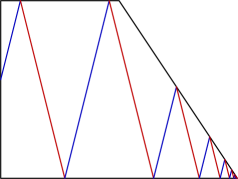
Figure 7. Left: a domain with corners and its $\varepsilon$-rounding (in blue). The circles have radius $\varepsilon$. Right: a trajectory on a trapezium which converges to a corner.

We next extend the concept of $\lambda$-simplicity to domains with corners. Let $\ell\in C^{\infty}(\mathbb{R}^{2};\mathbb{R})$ and $x=\mathbf{x}(\theta_{j})$ be a corner of $\Omega$. Consider the one-sided derivatives $\partial_{\theta}(\ell\circ\mathbf{x})(\theta_{j}\pm 0)$. There are three possible cases:

1. Both derivatives are nonzero and have the same sign – then we call $x$ not a critical point of $\ell$;

2. Both derivatives are nonzero and have opposite signs – then we call $x$ a nondegenerate critical point of $\ell$.

3. At least one of the derivatives is zero – then we call $x$ a degenerate critical point of $\ell$.

If $x=\mathbf{x}(\theta)$ is instead a regular point of the boundary, then we use the standard definition of critical points: $x$ is a critical point of $\ell$ if $\partial_{\theta}(\ell\circ\mathbf{x})(\theta)=0$, and a critical point is nondegenerate if $\partial_{\theta}^{2}(\ell\circ\mathbf{x})(\theta)\neq 0$. With the above convention for critical points, we follow Definition 1: we say that a domain with corners $\Omega$ is $\lambda$-simple if each of the functions $\ell^{\pm}(\bullet,\lambda)$ defined in (1.2) has exactly 2 critical points on $\partial\Omega$, which are both nondegenerate.

If $\Omega$ is $\lambda$-simple, then the involutions $\gamma^{\pm}(\bullet,\lambda):\partial\Omega\to\partial\Omega$ from (1.3) are well-defined and Lipschitz continuous. Thus $b=\gamma^{+}\circ\gamma^{-}$ is an orientation preserving bi-Lipschitz homeomorphism of $\partial\Omega$. We now revise the Morse–Smale conditions of Definition 2 as follows:

Definition 3.

Let $\Omega$ be a domain with corners. We say that $\lambda\in(0,1)$ satisfies the Morse–Smale conditions if:

1. $\Omega$ is $\lambda$-simple;

2. the set $\Sigma_{\lambda}$ of periodic points of the map $b(\bullet,\lambda)$ is nonempty;

3. the set $\Sigma_{\lambda}$ does not contain any corners of $\Omega$;

4. for each $x\in\Sigma_{\lambda}$, $\partial_{x}b^{n}(x,\lambda)\neq 1$ where $n$ is the minimal period.

The new condition (3) in Definition 3 ensures that $b$ is smooth near the $\gamma^{\pm}$-invariant set $\Sigma_{\lambda}$, so condition (4) makes sense. Without this condition we could have trajectories of $b$ converging to a corner, see Figure 7.

We finally show that if $\Omega$ is a domain with corners satisfying the Morse–Smale conditions of Definition 3 then an appropriate ‘rounding’ of $\Omega$ satisfies the Morse–Smale conditions of Definition 2:

Proposition 2.10.

Let $\Omega$ be a domain with corners and $\lambda\in(0,1)$ satisfy the Morse–Smale conditions for $\Omega$. Then there exists $\varepsilon>0$ such that for any open simply connected $\widehat{\Omega}\subset\mathbb{R}^{2}$ with $C^{\infty}$ boundary and such that:

• $\widehat{\Omega}$ is an $\varepsilon$-rounding of $\Omega$ in the sense that for each $x\in\mathbb{R}^{2}$ which lies distance $\geq\varepsilon$ from all the corners of $\Omega$, we have $x\in\Omega\iff x\in\widehat{\Omega}$; and

• the domain $\widehat{\Omega}$ is $\lambda$-simple in the sense of Definition 1,

the Morse–Smale conditions is satisfied for $\lambda$ and $\widehat{\Omega}$.

Proof.

Fix a parametrization $\mathbf{x}(\theta)$ of $\partial\Omega$ as in (2.28). Take a parametrization

$$\theta\in\mathbb{S}^{1}\quad\mapsto\quad\hat{\mathbf{x}}(\theta)\in\partial\widehat{\Omega}$$

which coincides with $\mathbf{x}(\theta)$ except $\varepsilon$-close to the corners:

$$\hat{\mathbf{x}}(\theta)=\mathbf{x}(\theta)\quad\text{for all}\quad\theta\notin\bigcup_{j=1}^{m}I_{j}(\varepsilon),\quad I_{j}(\varepsilon):=[\theta_{j}-C\varepsilon,\theta_{j}+C\varepsilon].$$ (2.29)

Here $C$ denotes a constant depending on $\Omega$ and the parametrization $\mathbf{x}(\theta)$, but not on $\widehat{\Omega}$ or $\varepsilon$, whose precise value might change from place to place in the proof.

Denote by $\gamma^{\pm},\hat{\gamma}^{\pm}$ the involutions (1.3) corresponding to $\Omega,\widehat{\Omega}$, and consider them as homeomorphisms of $\mathbb{S}^{1}$ using the parametrizations $x,\hat{x}$. Then by (2.29)

$$\gamma^{\pm}(\theta)=\hat{\gamma}^{\pm}(\theta)\quad\text{if}\quad\theta,\gamma^{\pm}(\theta)\not\in\bigcup_{j=1}^{m}I_{j}(\varepsilon).$$ (2.30)

Let $b=\gamma^{+}\circ\gamma^{-}$, $\hat{b}=\hat{\gamma}^{+}\circ\hat{\gamma}^{-}$ be the chess billiard maps of $\Omega,\widehat{\Omega}$ and $\Sigma_{\lambda},\widehat{\Sigma}_{\lambda}$ be the corresponding sets of periodic trajectories. Choose $\varepsilon>0$ such that the intervals $I_{j}(\varepsilon)$ do not intersect $\Sigma_{\lambda}$; this is possible since $\Sigma_{\lambda}$ does not contain any corners of $\Omega$. Since $\Sigma_{\lambda}$ is invariant under $\gamma^{\pm}$, we see from (2.30) that $b=\hat{b}$ in a neighborhood of $\Sigma_{\lambda}$ and thus $\Sigma_{\lambda}\subset\widehat{\Sigma}_{\lambda}$. That is, the periodic points for the original domain $\Omega$ are also periodic points for the rounded domain $\widehat{\Omega}$, with the same period $n$. It also follows that $\partial_{x}\hat{b}^{n}(x,\lambda)=\partial_{x}b^{n}(x,\lambda)\neq 1$ for all $x\in\Sigma_{\lambda}$.

It remains to show that $\widehat{\Sigma}_{\lambda}\subset\Sigma_{\lambda}$, that is the rounding does not create any new periodic points for $\hat{b}$. Note that all periodic points have the same period $n$, and it is enough to show that

$$\hat{b}^{n}(\theta)\neq\theta\quad\text{for all}\quad\theta\in\bigcup_{j=1}^{m}I_{j}(\varepsilon).$$ (2.31)

From (2.30), the monotonicity of $\gamma^{\pm},\hat{\gamma}^{\pm}$, and the Lipschitz continuity of $\gamma^{\pm}$ we have

$$|\gamma^{\pm}(\theta)-\hat{\gamma}^{\pm}(\theta)|\leq C\varepsilon\quad\text{for all}\quad\theta\in\mathbb{S}^{1}.$$

Iterating this and using the Lipschitz continuity of $\gamma^{\pm}$ again, we get

$$|b^{n}(\theta)-\hat{b}^{n}(\theta)|\leq C\varepsilon\quad\text{for all}\quad\theta\in\mathbb{S}^{1}.$$

Since $b^{n}(\theta_{j})\neq\theta_{j}$ for all $j=1,\dots,m$, taking $\varepsilon$ small enough we get (2.31), finishing the proof. ∎

2.5. Examples of Morse–Smale chess billiards

Here we present two examples of Morse–Smale chess billiards.

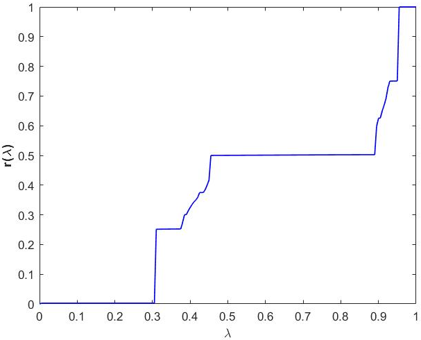
Figure 8. Left: the chess billiard for $\Omega_{\alpha}$ in Example 1. The numbers in bold mark the values of the coordinate $\theta$ at the vertices. Right: rotation numbers as functions of $\lambda$ for $\Omega_{\pi/10}$.

Example 1. For $\alpha\in(0,\frac{\pi}{2})$, let $\Omega_{\alpha}\subset\mathbb{R}^{2}$ be the open square with vertices $(0,0)$, $(\cos{\alpha},\sin{\alpha})$, $\sqrt{2}(\cos(\alpha+\frac{\pi}{4}),\sin(\alpha+\frac{\pi}{4}))$, $(\cos(\alpha+\frac{\pi}{2}),\sin(\alpha+\frac{\pi}{2}))$. (See Figure 8.) We parametrize $\partial\Omega_{\alpha}$ by $\theta\in\mathbb{R}/4\mathbb{Z}$ so that the parametrization $\mathbf{x}(\theta)$ is affine on each side of the square and the vertices listed above correspond to $\theta=0,1,2,3$ respectively. For $\lambda\in(0,1)$, we define

$$\beta\in(0,{\pi}/{2}),\quad\tan{\beta}={\sqrt{1-\lambda^{2}}}/\lambda,\quad t_{1}:=\tan(\beta-\alpha),\quad t_{2}:=\tan(\beta+\alpha).$$

We will show that if

$$0<\alpha<{\pi}/{8},\ \ {\pi}/{4}-\alpha<\beta<{\pi}/{4}+\alpha,$$

or equivalently

$$0<\alpha<{\pi}/{8},\ \ \cos({\pi}/{4}+\alpha)<\lambda<\cos({\pi}/{4}-\alpha),$$ (2.32)

then $\lambda$ and $\Omega_{\alpha}$ satisfy the Morse–Smale conditions (Definition 3). Moreover, for $\alpha$, $\lambda$ satisfying (2.32), we have (identifying $\theta$ with $\mathbf{x}(\theta)$)

$$\Sigma_{\lambda}=\left\{\tfrac{1-t_{1}}{t_{2}-t_{1}},\ \ 1+\tfrac{t_{1}(t_{2}-1)}{t_{2}-t_{1}},\ \ 2+\tfrac{1-t_{1}}{t_{2}-t_{1}},\ \ 3+\tfrac{t_{1}(t_{2}-1)}{t_{2}-t_{1}}\right\},$$ (2.33)

and the rotation number is $\mathbf{r}(\lambda)=\tfrac{1}{2}$.

In fact, assume $\alpha$, $\lambda$ satisfy (2.32), then $\ell^{+}(\bullet,\lambda)$ has exactly two nondegenerate critical points $\mathbf{x}(0)$, $\mathbf{x}(2)$ on $\partial\Omega_{\alpha}$; $\ell^{-}(\bullet,\lambda)$ also has two nondegenerate critial points $\mathbf{x}(1),\mathbf{x}(3)$ on $\partial\Omega$. This shows that $\Omega_{\alpha}$ is $\lambda$-simple.

We have the following partial computation of the reflection maps $\gamma^{\pm}$ (note that $0<t_{1}<1<t_{2}<\infty$ by (2.32)):

$$\gamma^{+}(\theta) =\begin{cases}t_{2}^{-1}(2-\theta)+2,&1\leq\theta\leq 2,\\ t_{2}^{-1}(4-\theta),&3\leq\theta\leq 4;\end{cases}$$ (2.34)

$$\gamma^{-}(\theta) =\begin{cases}t_{1}(1-\theta)+1,&0\leq\theta\leq 1,\\ t_{1}(3-\theta)+3,&2\leq\theta\leq 3.\end{cases}$$

This in particular implies that we have the mapping properties

$$[0,1]\xrightarrow{\gamma^{-}}[1,2]\xrightarrow{\gamma^{+}}[2,3]\xrightarrow{\gamma^{-}}[3,4]\xrightarrow{\gamma^{+}}[0,1].$$ (2.35)

Recall that $b=\gamma^{+}\circ\gamma^{-}$. We compute

$$b^{2}(\theta)=\left({t_{1}}/{t_{2}}\right)^{2}\theta+{(t_{1}+t_{2})(1-t_{1})}/{t_{2}^{2}},\ \ \theta\in[0,1].$$ (2.36)

By solving $b^{2}(\theta_{0})=\theta_{0}$, $\theta_{0}\in[0,1]$, we find $\theta_{0}=({1-t_{1}})/({t_{2}-t_{1}})$ and

$$\{\theta_{0},\ \gamma^{-}(\theta_{0}),\ b(\theta_{0}),\ \gamma^{+}(\theta_{0})\}\subset\Sigma_{\lambda}.$$

This shows that the right-hand side of (2.33) lies in $\Sigma_{\lambda}$ and that the rotation number is $\mathbf{r}(\lambda)={1\over 2}$. On the other hand, suppose $\theta_{1}\in\mathbb{R}/4\mathbb{Z}$ and $\theta_{1}\in\Sigma_{\lambda}$. If $\theta_{1}\in[0,1]$, then $\theta_{1}=\theta_{0}$ by (2.36). If $\theta_{1}\in[2,3]$, then $b(\theta_{1})\in\Sigma_{\lambda}\cap[0,1]$ and thus $\theta_{1}=b(\theta_{0})$. If $\theta_{1}\in[1,2]$, then $\gamma^{+}(\theta_{1})\in\Sigma_{\lambda}\cap[2,3]$ and thus $\theta_{1}=\gamma^{-}(\theta_{0})$. Finally, if $\theta_{1}\in[3,4]$, then $\gamma^{+}(\theta_{1})\in\Sigma_{\lambda}\cap[0,1]$ and thus $\theta_{1}=\gamma^{+}(\theta_{0})$. This shows (2.33).

Using (2.36) and the fact that $b^{2}$ commutes with $b$ and is conjugated by $\gamma^{\pm}$ to $b^{-2}$ we compute

$$\partial_{\theta}b^{2}(\theta)=\begin{cases}t_{1}^{2}/t_{2}^{2}<1,&\theta\in\{\theta_{0},b(\theta_{0})\};\\ t_{2}^{2}/t_{1}^{2}>1,&\theta\in\{\gamma^{-}(\theta_{0}),\gamma^{+}(\theta_{0})\}.\end{cases}$$

We have now checked that under the condition (2.32), $\Omega_{\alpha}$ and $\lambda$ satisfy all conditions in Definition 3.

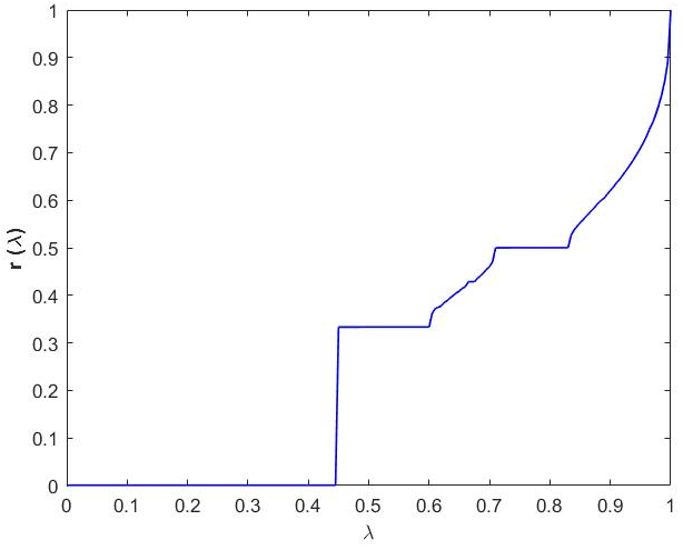
Figure 9. Left: the chess billiard for $\mathcal{T}_{d}$ in Example 2. Right: rotation numbers as functions of $\lambda$ for $\mathcal{T}_{1/2}$.

Example 2. Let $\mathcal{T}_{d}\subset\mathbb{R}^{2}$ be the open trapezium with vertices $(0,0)$, $(1+d,0)$, $(1,1)$, $(0,1)$, $d>0$. (See Figure 9.) We parametrize $\partial\mathcal{T}_{d}$ by $\theta\in\mathbb{R}/4\mathbb{Z}$ so that the parametrization $\mathbf{x}(\theta)$ is affine on each side of the trapezium and the vertices listed above correspond to $\theta=0,1,2,3$ respectively.

For $\lambda\in(0,1)$, we put $c=\lambda/\sqrt{1-\lambda^{2}}$. We assume that

$$\max(1,d)<c<d+1.$$ (2.37)

Under the condition (2.37) we know $\ell^{+}(\bullet,\lambda)$ has exactly two nondegenerate critial points $\mathbf{x}(0)$, $\mathbf{x}(2)$; $\ell^{-}(\bullet,\lambda)$ also has two nondegenerate critical points $\mathbf{x}(1)$, $\mathbf{x}(3)$. Hence $\mathcal{T}_{d}$ is $\lambda$-simple.

We have the following partial computation of the reflection maps $\gamma^{\pm}$:

$$\gamma^{+}(\theta) =\begin{cases}2+(c-d)(2-\theta),&1\leq\theta\leq 2,\\ {c\over 1+d}(4-\theta),&3\leq\theta\leq 4;\end{cases}$$ (2.38)

$$\gamma^{-}(\theta) =\begin{cases}{1+d\over c+d}(1-\theta)+1,&0\leq\theta\leq 1,\\ {1\over c}(3-\theta)+3,&2\leq\theta\leq 3.\end{cases}$$

This in particular implies that we again have the mapping properties (2.35). From here we compute

$$b^{2}(\theta)=\frac{c-d}{c+d}\theta+\frac{2c(c-1)}{(1+d)(c+d)},\quad\theta\in[0,1].$$

The fixed point of this map is

$$\theta_{0}=\frac{c(c-1)}{d(1+d)}.$$

Arguing as in Example 1, we see that $\mathcal{T}_{d}$, $\lambda$ satisfy the conditions of Definition 3, with

$$\Sigma_{\lambda}=\{\textstyle{c(c-1)\over d(1+d)},\ 2-{c-1\over d},\ 3-c+{c(c-1)\over d},\ 4-{c-1\over d}\}.$$

3. Microlocal preliminaries

In this section we present some general results needed in the proof. Most of the microlocal analysis in this paper takes place on the one dimensional boundary $\partial\Omega$; we review the basic notions in §3.1. In §3.2 we review definitions and basic properties of conormal distributions (needed in dimensions one and two). These are used to prove and formulate Theorem 1: the singularities of $(P-\lambda^{2}\mp i0)^{-1}f$ using conormal distributions. In our approach, this structure of $(P-\lambda^{2}\mp i0)^{-1}f$ is essential for describing the long time evolution profile in Theorem 2. Finally, §§3.3–3.4 contain technical results needed in §4.

3.1. Microlocal analysis on $\partial\Omega$

We first briefly discuss pseudodifferential operators on the circle $\mathbb{S}^{1}=\mathbb{R}/\mathbb{Z}$, referring to [19, §18.1] for a detailed introduction to the theory of pseudodifferential operators. Pseudodifferential operators on $\mathbb{S}^{1}$ are given by quantizations of 1-periodic symbols. More precisely, if $0\leq\delta<{1\over 2}$ and $m\in\mathbb{R}$, then we say that $a\in C^{\infty}(\mathbb{R}^{2})$ lies in $S^{m}_{\delta}(T^{*}\mathbb{S}^{1})$ if (denoting $\langle\xi\rangle:=\sqrt{1+|\xi|^{2}}$)

$$a(x+1,\xi)=a(x,\xi),\ \ |\partial_{x}^{\alpha}\partial_{\xi}^{\beta}a(x,\xi)|\leq C_{\alpha\beta}\langle\xi\rangle^{m+\delta\alpha-(1-\delta)\beta}.$$ (3.1)

For brevity we just write $S^{m}_{\delta}:=S^{m}_{\delta}(T^{*}\mathbb{S}^{1})$. Each $a\in S^{m}_{\delta}$ is quantized by the operator $\operatorname{Op}(a):C^{\infty}(\mathbb{S}^{1})\to C^{\infty}(\mathbb{S}^{1})$, $\mathcal{D}^{\prime}(\mathbb{S}^{1})\to\mathcal{D}^{\prime}(\mathbb{S}^{1})$ defined by

$$\operatorname{Op}(a)u(x)=\frac{1}{2\pi}\int_{\mathbb{R}^{2}}e^{i(x-y)\xi}a(x,\xi)u(y)\,dyd\xi,$$ (3.2)

where $u\in C^{\infty}(\mathbb{R})$ is 1-periodic and the integral is understood in the sense of oscillatory integrals [18, §7.8]. We introduce the following spaces of pseudodifferential operators:

$$\Psi_{\delta}^{m}:=\{\operatorname{Op}(a):a\in S^{m}_{\delta}\},\quad\Psi^{m+}_{\delta}=\bigcap_{m^{\prime}>m}\Psi^{m^{\prime}}_{\delta},\quad\Psi^{m}_{\delta+}=\bigcap_{\delta^{\prime}>\delta}\Psi^{m}_{\delta^{\prime}},$$

$$S^{m+}_{\delta}=\bigcap_{m^{\prime}>m}S^{m^{\prime}}_{\delta},\quad S^{m}_{\delta+}=\bigcap_{\delta^{\prime}>\delta}S^{m}_{\delta^{\prime}}.$$

We remark that $S^{m}_{\delta+}\subset S^{m+}_{\delta}$; moreover, $a\in S^{m+}_{\delta}$ lies in $S^{m}_{\delta+}$ if and only if $a(x,\xi)=\mathcal{O}(\langle\xi\rangle^{m})$. We henceforth denote $\Psi^{m}:=\Psi^{m}_{0}$. The space $\Psi^{-\infty}:=\bigcap_{m}\Psi^{m}$ consists of smoothing operators.

In terms of Fourier series on $\mathbb{S}^{1}$, we have

$$\begin{gathered}\operatorname{Op}(a)u(x)=\sum_{k,n\in\mathbb{Z}}e^{2\pi inx}a_{n-k}(k)u_{k},\\ a_{\ell}(k):=\int_{0}^{1}a(x,2\pi k)e^{-2\pi i\ell x}\,dx,\ \ \ u_{k}:=\int_{0}^{1}u(x)e^{-2\pi ikx}\,dx.\end{gathered}$$ (3.3)

This shows that $\operatorname{Op}(a)$ does not determine $a$ uniquely. This representation also shows boundedness on Sobolev spaces $\operatorname{Op}(a):H^{s}(\mathbb{S}^{1})\to H^{s-m}(\mathbb{S}^{1})$, $s\in\mathbb{R}$, $a\in S^{m}_{\delta}$. Indeed, smoothness of $a$ in $x$ shows that $a_{\ell}(k)=\mathcal{O}(\langle\ell\rangle^{-\infty}\langle k\rangle^{m})$ and the bound on the norm follows from the Schur criterion [12, (A.5.3)]. Despite the fact that $A:=\operatorname{Op}(a)$ does not determine $a$ uniquely, it does determine its essential support, which is the right hand side in the definition of the wave front set of a pseudodifferential operator:

$$\operatorname{WF}(A):=\complement\{(x,\xi):\xi\neq 0,\,\exists\,\rho>0:a(y,\eta)=\mathcal{O}(\langle\eta\rangle^{-\infty})\text{ when }|x-y|<\rho,\ \tfrac{\eta}{\xi}>0\},$$

see [12, §E.2]. We refer to that section and [19, §18.1] for a discussion of wave front sets. We also recall a definition of the wave front set of a distribution,

$$\begin{gathered}\operatorname{WF}(u):=\bigcap_{Au\in C^{\infty},A\in\Psi^{0}}{\rm{Char}}(A),\\ {\rm{Char}}(A):=\complement\{(x,\xi):\xi\neq 0,\,\exists\,\rho,c>0:|a(y,\eta)|>c,\ \ |x-y|<\rho,\ \tfrac{\eta}{\xi}>0,\ |\eta|>1/\rho\}\end{gathered}$$

The symbol calculus on $\mathbb{S}^{1}$ translates directly from the symbol calculus of pseudodifferential operators on $\mathbb{R}$. We record in particular the composition formula [19, Theorem 18.1.8]: for $b_{1}\in S^{m_{1}}_{\delta}$, $b_{2}\in S^{m_{2}}_{\delta}$,

$$\begin{gathered}\operatorname{Op}(b_{1})\operatorname{Op}(b_{2})=\operatorname{Op}(b),\ \ \ b\in S^{m_{1}+m_{2}}_{\delta},\\ b(x,\xi)=\exp(-i\partial_{y}\partial_{\eta})\left[b_{1}(x,\eta)b_{2}(y,\xi)\right]|_{(y,\eta)=(x,\xi)},\\ b(x,\xi)=\sum_{0\leq k<N}\frac{(-i)^{k}}{k!}\partial_{\xi}^{k}b_{1}(x,\xi)\partial_{x}^{k}b_{2}(x,\xi)+b_{N}(x,\xi),\ \ b_{N}\in S^{m-N(1-2\delta)}_{\delta}.\end{gathered}$$ (3.4)

where expanding the exponential gives an asymptotic expansion of $b$.

We record here a norm bound for pseudodifferential operators at high frequency:

Lemma 3.1.

Assume that $a\in S^{0}_{\delta}$, $r\in S^{-1+}$, and $\sup|a|\leq R$. Then for all $N$, $\nu>0$, and $u\in L^{2}(\mathbb{S}^{1})$ we have

$$\|\operatorname{Op}(a+r)u\|_{L^{2}}\leq(R+\nu)\|u\|_{L^{2}}+C\|u\|_{H^{-N}}$$ (3.5)

where the constant $C$ depends on $R$, $\nu$, $N$, and some seminorms of $a$ and $r$ but not on $u$.

Proof.

By [16, Lemma 4.6] we can write

$$(R+\nu)^{2}I=\operatorname{Op}(a+r)^{*}\operatorname{Op}(a+r)+\operatorname{Op}(b)^{*}\operatorname{Op}(b)+\operatorname{Op}(q)$$

for some $b\in S^{0}_{\delta}$ and $q\in S^{-\infty}$. The bound (3.5) follows. ∎

Although $a$ in (3.3) is not unique, the principal symbol of $\operatorname{Op}(a)$ defined as

$$\sigma(\operatorname{Op}(a))=[a]\in S^{m}_{\delta}/S^{m-1+2\delta}_{\delta}$$ (3.6)

is, and we have a short exact sequence $0\to\Psi_{\delta}^{m-1+2\delta}\to\Psi_{\delta}^{m}\xrightarrow{\sigma}S^{m}_{\delta}/S^{m-1+2\delta}_{\delta}\to 0$. Somewhat informally, we write $\sigma(\operatorname{Op}(a))=b$ for any $b$ satisfying $a-b\in S^{m-1+2\delta}_{\delta}$.

In our analysis, we also consider families $\varepsilon\mapsto a_{\varepsilon}$, $\varepsilon\geq 0$, such that $a_{\varepsilon}\in S^{-\infty}$ for $\varepsilon>0$ and $a_{0}\in S^{m}_{\delta}$. In that case, for $A_{\varepsilon}=\operatorname{Op}(a_{\varepsilon})$,

$$\sigma(A_{\varepsilon})=[b_{\varepsilon}],\ \ \ b_{\varepsilon}-a_{\varepsilon}\in S^{m-1+2\delta}_{\delta}\ \text{ uniformly for $\varepsilon\geq 0$.}$$ (3.7)

Again, we drop $[\bullet]$ when writing $\sigma(A)$ for a specific operator.

We will crucially use mild exponential weights which result in pseudodifferential operators of varying order – see [36], and in a related context, [14].

Lemma 3.2.

Suppose that (in the sense of (3.1)) $m_{j}\in S^{0}$, $m_{0}$ is real-valued, and

$$G(x,\xi):=m_{0}(x,\xi)\log\langle\xi\rangle+m_{1}(x,\xi),\ \ \ m_{0}(x,t\xi)=m_{0}(x,\xi),\ \ t,|\xi|\geq 1.$$ (3.8)

Then

$$e^{G}\in S^{M}_{0+},\quad e^{-G}\in S^{-m}_{0+},\ \ \ M:=\max_{|\xi|=1}m_{0}(x,\xi),\ \ \ m:=\min_{|\xi|=1}m_{0}(x,\xi),$$ (3.9)

and there exists $r_{G}\in S^{-1+}$ such that

$$\begin{gathered}\operatorname{Op}(e^{G})\operatorname{Op}(e^{-G}(1+r_{G}))-I,\ \operatorname{Op}(e^{-G}(1+r_{G}))\operatorname{Op}(e^{G})-I\in\Psi^{-\infty}.\end{gathered}$$ (3.10)

Also, if $G_{j}(x,\xi)$ are given by (3.8) with $m_{0}$ and $m_{1}$ replaced by $m_{0j}$, $m_{1j}$, respectively, then for $a_{j}\in S^{0}$, $r_{j}\in S^{-1+}$, $j=1,2$, there exists $r_{3}\in S^{-1+}$ such that

$$\operatorname{Op}(e^{G_{1}}(a_{1}+r_{1}))\operatorname{Op}(e^{G_{2}}(a_{2}+r_{2}))=\operatorname{Op}(e^{G_{1}+G_{2}}(a_{1}a_{2}+r_{3})).$$ (3.11)

Proof.

Since $\log\langle\xi\rangle=\mathcal{O}_{\varepsilon}(\langle\xi\rangle^{\varepsilon})$ for all $\varepsilon>0$, (3.9) follows from (3.1). In fact, we have the stronger bound

$$|\partial^{\alpha}_{x}\partial^{\beta}_{\xi}(e^{\pm G(x,\xi)})|\leq C_{\alpha\beta\varepsilon}e^{\pm G(x,\xi)}\langle\xi\rangle^{\varepsilon-|\beta|},\quad\varepsilon>0.$$ (3.12)

This gives (3.11). Indeed, the remainder in the expansion (3.4) is in $S^{M_{1}+M_{2}-N+}$ and the $k$-th term is in $e^{G_{1}+G_{2}}S^{-k+}$ by (3.12); it suffices to take $N\geq M+M_{2}+1$.

To obtain (3.10) we note that (3.11) gives $\operatorname{Op}(e^{\pm G})\operatorname{Op}(e^{\mp G})=I-\operatorname{Op}(r_{\pm})$, $r_{\pm}\in S^{-1+}$. We then have parametrices for the operators $I-\operatorname{Op}(r_{\pm})$ [19, Theorem 18.1.9], $I+\operatorname{Op}(b_{\pm})$, which give left and right approximate inverses (in the sense of (3.10)) $(I+\operatorname{Op}(b_{-}))\operatorname{Op}(e^{-G})$, $\operatorname{Op}(e^{-G})(I+\operatorname{Op}(b_{+}))$. Those have the required form by (3.11) (where one of $G_{1},G_{2}$ is equal to $-G$ and the other one is equal to 0). ∎

We also record a change of variables formula. Suppose $f:\mathbb{R}/\mathbb{Z}\to\mathbb{R}/\mathbb{Z}$ is a diffeomorphism with a lift $\mathbf{f}:\mathbb{R}\to\mathbb{R}$, $\mathbf{f}(x+1)=\mathbf{f}(x)\pm 1$ (with the $+$ sign for orientation preserving $f$ and the $-$ sign otherwise). For symbols 1-periodic in $x$ we can use the standard formula given in [19, Theorem 18.1.17] and an argument similar to (3.11). That gives, for $G$ given by (3.8), and $r\in S^{-1+}$,

$$\begin{gathered}f^{*}\circ\operatorname{Op}(e^{G}(1+r))=\operatorname{Op}(e^{G_{f}}(1+r_{f}))\circ f^{*},\\ G_{f}(x,\xi):=G(f(x),f^{\prime}(x)^{-1}\xi),\ \ r_{f}\in S^{-1+}.\end{gathered}$$ (3.13)

In §4.6 below we will use pseudodifferential operators acting on 1-forms on $\mathbb{S}^{1}$. Using the canonical 1-form $dx$, $x\in\mathbb{S}^{1}=\mathbb{R}/\mathbb{Z}$, we identify 1-forms with functions, and this gives an identification of the class $\Psi^{m}_{\delta}(\mathbb{S}^{1};T^{*}\mathbb{S}^{1})$ (operators acting on 1-forms) with $\Psi^{m}_{\delta}(\mathbb{S}^{1})$ (operators acting on functions). This defines the principal symbol map, which we still denote by $\sigma$.

Fixing a positively oriented coordinate $\theta:\partial\Omega\to\mathbb{S}^{1}$, we can identify functions / distributions on $\partial\Omega$ with functions / distributions on $\mathbb{S}^{1}$. The change of variables formula used for (3.13) also shows the invariance of $\sigma(A)$ under changes of variables and allows pseudodifferential operators acting on section of bundles – see [19, Definition 18.1.32]. In particular, we can define the class of pseudodifferential operators $\Psi^{m}_{\delta}(\partial\Omega;T^{*}\partial\Omega)$ acting on 1-forms on $\partial\Omega$ and the symbol map

$$\sigma:\Psi^{m}_{\delta}(\partial\Omega;T^{*}\partial\Omega)\to S^{m}_{\delta}(T^{*}\partial\Omega)/S^{m-1+2\delta}_{\delta}(T^{*}\partial\Omega),$$ (3.14)

with the class $\Psi^{m}_{\delta}$ and the map $\sigma$ independent of the choice of coordinate on $\partial\Omega$.

3.2. Conormal distributions

We now review conormal distributions associated to hypersurfaces, referring the reader to [19, §18.2] for details. Although we consider the case of manifolds with boundaries, the hypersurfaces are assumed to be transversal to the boundaries and conormal distributions are defined as restrictions of conormal distributions in the no-boundary case.

Let $M$ be a compact $m$-dimensional manifold with boundary and $\Sigma\subset M$ be a compact hypersurface transversal to the boundary (that is, $\Sigma$ is a compact codimension 1 submanifold of $M$ with boundary $\partial\Sigma=\Sigma\cap\partial M$ and $T_{x}\Sigma\neq T_{x}\partial M$ for all $x\in\partial\Sigma$). We should emphasize that in our case, the hypersurfaces $\Sigma$ take a particularly simple form: we either have $M=\overline{\Omega}$ and $\Sigma$ given by straight lines transversal to $\partial\Omega$ (see Theorems 1 and 2) or $M=\partial\Omega\simeq\mathbb{S}^{1}$ and $\Sigma$ is given by points (see Propositions 7.3 and 7.4).

The conormal bundle to $\Sigma$ is given by $N^{*}\Sigma:=\{(x,\xi)\in T^{*}M\colon x\in\Sigma,\ \xi|_{T_{x}\Sigma}=0\}$, which is a Lagrangian submanifold of $T^{*}M$ and a one-dimensional vector bundle over $\Sigma$. For $k\in\mathbb{R}$, define the symbol class $S^{k}(N^{*}\Sigma)$ consisting of functions $a\in C^{\infty}(N^{*}\Sigma)$ satisfying the derivative bounds

$$|\partial_{x}^{\alpha}\partial_{\theta}^{\beta}a(x,\theta)|\leq C_{\alpha\beta}\langle\theta\rangle^{k-|\beta|}$$ (3.15)

where we use local coordinates $(x,\theta)\in\mathbb{R}^{m-1}\times\mathbb{R}\simeq N^{*}\Sigma$. Here $x$ is a coordinate on $\Sigma$ and $\theta$ is a linear coordinate on the fibers of $N^{*}\Sigma$; $\langle\theta\rangle:=\sqrt{1+|\theta|^{2}}$. The estimates (3.15) are supposed to be valid uniformly up to the boundary of $\Sigma$. In other words we can consider $a$ as a restriction of a symbol defined on an extension of $\Sigma$.

Denote by $I^{s}(M,N^{*}\Sigma)\subset\overline{\mathcal{D}^{\prime}}(M^{\circ})$ the space of extendible distributions on the interior $M^{\circ}$ (see [19, §B.2]) which are conormal to $\Sigma$ of order $s\in\mathbb{R}$ smoothly up to the boundary of $M$. To describe the class $I^{s}$ we first consider two model cases:

• if $M=\mathbb{R}^{m}$, we write points in $\mathbb{R}^{m}$ as $(x_{1},x^{\prime})\in\mathbb{R}\times\mathbb{R}^{m-1}$, and $\Sigma=\{x_{1}=0\}$, then a compactly supported distribution $u\in\mathcal{E}^{\prime}(\mathbb{R}^{m})$ lies in $I^{s}(M,N^{*}\Sigma)$ if and only its Fourier transform in the $x_{1}$ variable, $\check{u}(\xi_{1},x^{\prime})$, lies in $S^{{m\over 4}-{1\over 2}+s}(N^{*}\Sigma)$ where $N^{*}\Sigma=\{(0,x^{\prime},\xi_{1},0)\mid x^{\prime}\in\mathbb{R}^{m-1},\ \xi_{1}\in\mathbb{R}\}$.

• if $M=\mathbb{R}_{x_{1}}\times[0,\infty)_{x_{2}}\times\mathbb{R}^{m-2}_{x^{\prime\prime}}$ and $\Sigma=\{x_{1}=0,\ x_{2}\geq 0\}$, then a distribution $u\in\mathcal{D}^{\prime}(M^{\circ})$ with bounded support lies in $I^{s}(M,N^{*}\Sigma)$ if and only if $u=\tilde{u}|_{M^{\circ}}$ for some $\tilde{u}\in\mathcal{E}^{\prime}(\mathbb{R}^{m})$ which lies in $I^{s}(\mathbb{R}^{m},N^{*}\widetilde{\Sigma})$, with $\widetilde{\Sigma}:=\{x_{1}=0\}\subset\mathbb{R}^{m}$. Alternatively, $\check{u}(\xi_{1},x^{\prime})$ lies in $S^{{m\over 4}-{1\over 2}+s}(N^{*}\Sigma)$ where the derivative bounds are uniform up to the boundary.

In those model cases, elements of $I^{s}(M,N^{*}\Sigma)$ are given by the oscillatory integrals (where we use the prefactor from [19, Theorem 18.2.9])

$$u(x)=(2\pi)^{-\frac{m}{4}-\frac{1}{2}}\int_{\mathbb{R}}e^{ix_{1}\xi_{1}}a(x^{\prime},\xi_{1})\,d\xi_{1},\ \ a\in S^{\frac{m}{4}-\frac{1}{2}+s}(N^{*}\{x_{1}=0\}).$$ (3.16)

We note that in both of the above cases the distribution $u$ is in $C^{\infty}(M)$ (up to the boundary in the second case) outside of any neighborhood of $\Sigma$.

For the case of general compact manifold $M$ and hypersurface $\Sigma$ transversal to the boundary of $M$, we say that $u\in I^{s}(M,N^{*}\Sigma)$ if (see [19, Theorem 18.2.8])

1. $u$ is in $C^{\infty}(M)$ (up to the boundary) outside of any neighborhood of $\Sigma$; and

2. the localizations of $u$ to the model cases using coordinates lie in $I^{s}$ as defined above.

Note that the wavefront set of any $u\in I^{s}(M,N^{*}\Sigma)$, considered as a distribution on the interior $M^{\circ}$, is contained in $N^{*}\Sigma$.

In addition we define the space

$$I^{s+}(M,N^{*}\Sigma):=\bigcap_{s^{\prime}>s}I^{s^{\prime}}(M,N^{*}\Sigma).$$

Such spaces are characterized in terms of the Sobolev spaces (where for simplicity assume that $M$ has no boundary, since this is the only case used in this paper), $H^{s-}(M):=\bigcap_{s^{\prime}<s}H^{s^{\prime}}(M)$, as follows:

$$u\in I^{s+}(M,N^{*}\Sigma)\ \Longleftrightarrow\ \left\{\begin{array}[]{l}\text{ For any vector fields on~{}$M$ tangent to $\Sigma$,}\ X_{1},\dots,X_{\ell},\\ \quad X_{1}\dots X_{\ell}\,u\in H^{-{m\over 4}-s-}(M),\end{array}\right.$$ (3.17)

see [19, Definition 18.2.6 and Theorem 18.2.8].

Assume now that the conormal bundle $N^{*}\Sigma$ is oriented; for $(x,\xi)\in N^{*}\Sigma\setminus 0$ we say that $\xi>0$ if $\xi$ is positively oriented and $\xi<0$ if $\xi$ is negatively oriented. This gives the splitting

$$N^{*}\Sigma\setminus 0=N^{*}_{+}\Sigma\sqcup N^{*}_{-}\Sigma,\quad N^{*}_{\pm}\Sigma:=\{(x,\xi)\in N^{*}\Sigma\mid\pm\xi>0\}.$$ (3.18)

Denote by $I^{s}(M,N_{\pm}^{*}\Sigma)$ the space of distributions $u\in I^{s}(M,N^{*}\Sigma)$ such that $\operatorname{WF}(u)\subset N_{\pm}^{*}\Sigma$, up to the boundary. Since $\Sigma$ is transversal to the boundary this means that an extension of $u$ satisfies this condition. In the model case (and effectively in the cases considered in this paper) $M=\mathbb{R}^{m}$, $\Sigma=\{x_{1}=0\}$ they can be characterized as follows: $\check{u}(\xi_{1},x^{\prime})$ lies in $S^{{m\over 4}-{1\over 2}+s}(N^{*}\Sigma)$ and $\check{u}(\xi_{1},x^{\prime})=\mathcal{O}(\langle\xi_{1}\rangle^{-\infty})$ as $\xi_{1}\to\mp\infty$.

In the present paper we will often study the case when $M=\partial\Omega$, identified with $\mathbb{S}^{1}$ by a coordinate $\theta$, and we are given two finite sets $\Sigma^{+},\Sigma^{-}\subset\partial\Omega$ with $\Sigma^{+}\cap\Sigma^{-}=\emptyset$. We denote

$$I^{s}(\partial\Omega,N^{*}_{+}\Sigma^{-}\sqcup N^{*}_{-}\Sigma^{+}):=I^{s}(\partial\Omega,N^{*}_{+}\Sigma^{-})+I^{s}(\partial\Omega,N^{*}_{-}\Sigma^{+}).$$ (3.19)

Put $\Sigma:=\Sigma^{+}\sqcup\Sigma^{-}$, then $I^{s}(\partial\Omega,N^{*}_{+}\Sigma^{-}\sqcup N^{*}_{-}\Sigma^{+})$ consists of the elements of $I^{s}(\partial\Omega;N^{*}\Sigma)$ with wavefront set contained in $N^{*}_{+}\Sigma^{-}\sqcup N^{*}_{-}\Sigma^{+}$.

Assume that $\Sigma$ has an even number of points (which will be the case in our application) and fix a defining function $\rho\in C^{\infty}(\partial\Omega;\mathbb{R})$ of $\Sigma$: that is, $\Sigma=\rho^{-1}(0)$ and $d\rho\neq 0$ on $\Sigma$. Fix also a pseudodifferential operator $A_{\Sigma}\in\Psi^{0}(\partial\Omega)$ such that $\operatorname{WF}(A_{\Sigma})\cap(N^{*}_{+}\Sigma^{-}\sqcup N^{*}_{-}\Sigma^{+})=\emptyset$ and $A_{\Sigma}$ is elliptic on $N^{*}_{-}\Sigma^{-}\sqcup N^{*}_{+}\Sigma^{+}$. Using (3.17), we see that $u\in\mathcal{D}^{\prime}(\partial\Omega)$ lies in $I^{s+}(\partial\Omega,N^{*}_{+}\Sigma^{-}\sqcup N^{*}_{-}\Sigma^{+})$ if and only if the following seminorms are finite:

$$\|(\rho\partial_{\theta})^{N}u\|_{H^{-\frac{1}{4}-s-\beta}},\quad\|A_{\Sigma}u\|_{H^{N}}\quad\text{for all}\quad N\in\mathbb{N}_{0},\ \beta>0.$$ (3.20)

Choosing different $\rho$ and $A_{\Sigma}$ leads to an equivalent family of seminorms (3.20). In particular, if $\rho,A_{\Sigma}$ are as above and $\widetilde{A}_{\Sigma}\in\Psi^{0}(\partial\Omega)$ satisfies $\operatorname{WF}(\widetilde{A}_{\Sigma})\cap(N^{*}_{+}\Sigma^{-}\sqcup N^{*}_{-}\Sigma^{+})=\emptyset$ then $\operatorname{WF}(\widetilde{A}_{\Sigma})$ lies in the union of $\{\rho\neq 0\}$ and the elliptic set of $A_{\Sigma}$, thus by the elliptic estimate we have for $N_{0}\geq N+\frac{1}{4}+s+\beta$

$$\|\widetilde{A}_{\Sigma}u\|_{H^{N}}\leq C\big{(}\|A_{\Sigma}u\|_{H^{N}}+\|(\rho\partial_{\theta})^{N_{0}}u\|_{H^{-\frac{1}{4}-s-\beta}}+\|u\|_{H^{-\frac{1}{4}-s-\beta}}\big{)}.$$ (3.21)

Moreover, the operator $\rho\partial_{\theta}$ is bounded with respect to the seminorms (3.20), as are pseudodifferential operators in $\Psi^{0}(\partial\Omega)$ [19, Theorem 18.2.7].

We will also need the notion of conormal distributions depending smoothly on a parameter – see [13, Lemma 4.4] for a more general Lagrangian version. Here we restrict ourselves to the specific conormal distributions appearing in this paper and define relevant smooth families of conormal distributions in Proposition 7.4 and Lemma 8.3.

We will not discuss principal symbols of general conormal distributions to avoid introducing half-densities, however we give here a special case of the way the principal symbol changes under pseudodifferential operators and under pullbacks:

Lemma 3.3.

Assume that $u\in\mathcal{E}^{\prime}(\mathbb{R})$ lies in $I^{s}(\mathbb{R},\{0\})$, that is $\widehat{u}\in S^{s-\frac{1}{4}}(\mathbb{R})$. Then:

1. If $a(x,\xi)\in S^{0}(T^{*}\mathbb{R})$ is compactly supported in the $x$ variable and $\operatorname{Op}(a)$ is defined by (3.2), then

   $$\widehat{\operatorname{Op}(a)u}(\xi)=a(0,\xi)\widehat{u}(\xi)+S^{s-\frac{5}{4}}(\mathbb{R}).$$ (3.22)

2. If $f$ is a diffeomorphism of open subsets of $\mathbb{R}$ such that $f(0)=0$ and the range of $f$ contains $\operatorname{supp}u$, then

   $$\widehat{f^{*}u}(\xi)={1\over|f^{\prime}(0)|}\widehat{u}\Big{(}{\xi\over f^{\prime}(0)}\Big{)}+S^{s-\frac{5}{4}}(\mathbb{R}).$$ (3.23)

Proof.

Since these statements are standard, we only sketch the proofs, referring to [19, Theorems 18.2.9 and 18.2.12] for details. To see (3.22) we use the formula

$$\widehat{\operatorname{Op}(a)u}(\xi)={1\over 2\pi}\int_{\mathbb{R}^{2}}e^{ix(\eta-\xi)}a(x,\eta)\widehat{u}(\eta)\,d\eta dx.$$

Assume that $|\xi|\geq 1$. Using a smooth partition of unity, we split the integral above into 2 pieces: one where $|\eta-\xi|\geq\frac{1}{4}|\xi|$ and another one where $|\eta-\xi|\leq\frac{1}{2}|\xi|$. The first piece is rapidly decaying in $\xi$ by integration by parts in $x$. The second piece is equal to $a(0,\xi)\widehat{u}(\xi)+S^{s-\frac{5}{4}}(\mathbb{R})$ by the method of stationary phase.

To see (3.23) we fix a cutoff $\chi\in C^{\infty}_{\mathrm{c}}(\mathbb{R})$ such that $\operatorname{supp}\chi$ lies in the range of $f$ and $\chi=1$ near $\operatorname{supp}u$. Using the Fourier inversion formula, we write

$$\widehat{f^{*}u}(\xi)={1\over 2\pi}\int_{\mathbb{R}^{2}}e^{i(f(x)\eta-x\xi)}\chi(f(x))\widehat{u}(\eta)\,d\eta dx.$$

Now (3.23) is proved similarly to (3.22). Here in the application of the method of stationary phase, the critical point is given by $x=0$, $\eta=\xi/f^{\prime}(0)$ and the Hessian of the phase at the critical point has signature 0 and determinant $-f^{\prime}(0)^{2}$. ∎

3.3. Convolution with logarithm

In §4 we need information about mapping properties between spaces of conormal distributions on the boundary and conormal distributions in the interior. In preparation for Lemma 4.8 below we now prove the following

Lemma 3.4.

Let $f\in C^{\infty}_{\mathrm{c}}(\mathbb{R})$ and define

$$g(x):=\int_{0}^{\infty}\log|x-y|\,{f(y)\over\sqrt{y}}\,dy,\quad x>0.$$ (3.24)

Then $g\in C^{\infty}([0,\infty))$.

Remark. In general $g$ is not smooth on $(-\infty,0]$. In fact, changing variables $y=s^{2}|x|$, we obtain (see (3.25) below)

$$g^{\prime}(x)=-2|x|^{-\frac{1}{2}}\int_{0}^{\infty}\frac{f(s^{2}|x|)}{1+s^{2}}\,ds,\quad x<0,$$

which blows up as $x\to 0-$ if $f(0)\neq 0$. This, and the conclusion of Lemma 3.4, can also be seen from analysis on the Fourier transform side.

Proof.

Denote $x_{+}^{-1/2}:=H(x)x^{-1/2}$ where $H(x)$ is the Heaviside function: $H(x)=1$ for $x>0$ and $H(x)=0$ for $x<0$. Since $g$ is the convolution of $\log|x|$ and $x_{+}^{-1/2}f(x)$, which are both smooth except at $x=0$, the function $g$ is smooth on $(0,\infty)$. Thus it suffices to prove that $g$ is smooth on $[0,1]$ up to the boundary.

1. Assume first that $f$ is real valued and extends holomorphically to the disk $\{|z|<4\}$. Making the change of variables $y:=t^{2}$, we write

$$g(x)=2\int_{0}^{\infty}\log|t^{2}-x|f(t^{2})\,dt=\int_{\mathbb{R}}\log|t^{2}-x|f(t^{2})\,dt.$$ (3.25)

Assume that $x\in(0,1]$ and consider the holomorphic function

$$\psi_{x}(z):=\log(z-\sqrt{x})+\log(z+\sqrt{x}),\quad z\in\mathbb{C}\setminus\big{(}(\sqrt{x}-i[0,\infty))\cup(-\sqrt{x}-i[0,\infty))\big{)},$$

where we use the branch of the logarithm on $\mathbb{C}\setminus-i[0,\infty)$ which takes real values on $(0,\infty)$. Then $\operatorname{Re}\psi_{x}(t)=\log|t^{2}-x|$ for all $t\in\mathbb{R}\setminus\{\sqrt{x},-\sqrt{x}\}$.

Figure 10. The contour $\Gamma$ used in the proof of Lemma 3.4. The dashed lines are the cuts needed to define the function $\psi_{x}(z)$.

Fix an $x$-independent contour $\Gamma=\{t+iw(t)\mid t\in\mathbb{R}\}\subset\mathbb{C}$ such that $w(t)\geq 0$ everywhere, $w(t)=0$ for $|t|\geq{3\over 2}$, $|t+iw(t)|<2$ for $|t|\leq{3\over 2}$, and $w(t)>0$ for $|t|\leq 1$. (See Figure 10.) Deforming the contour in (3.25), we get

$$g(x)=\operatorname{Re}\int_{\Gamma}\psi_{x}(z)f(z^{2})\,dz\quad\text{for all}\quad x\in(0,1].$$

Since $\partial_{x}\psi_{x}(z)=(x-z^{2})^{-1}$, the function $\psi_{x}(z)$ and all its $x$-derivatives are bounded uniformly in $x\in(0,1]$ and locally uniformly in $z\in\Gamma$. It follows that $g$ is smooth on the interval $[0,1]$.

2. For the general case, fix a cutoff $\chi\in C^{\infty}_{\mathrm{c}}(\mathbb{R})$ such that $\chi=1$ near $[-4,4]$. Take arbitrary $N\in\mathbb{N}$. Using the Taylor expansion of $f$ at 0, we write

$$f(x)=f_{1}(x)+f_{2}(x),\quad f_{1}(x)=p(x)\chi(x)$$

where $p$ is a polynomial of degree at most $N$ and $f_{2}\in C^{\infty}_{\mathrm{c}}(\mathbb{R})$ satisfies $f_{2}(x)=\mathcal{O}(|x|^{N+1})$ as $x\to 0$. We write $g=g_{1}+g_{2}$ where $g_{j}$ are constructed from $f_{j}$ using (3.24).

By Step 1 of the present proof, we see that $g_{1}$ is smooth on $[0,1]$. On the other hand, $x_{+}^{-1/2}f_{2}(x)\in C^{N}(\mathbb{R})$; since $\log|x|$ is locally integrable we get $g_{2}\in C^{N}([0,1])$. Since $N$ can be chosen arbitrary, this gives $g\in C^{\infty}([0,1])$ and finishes the proof. ∎

We also give the following general mapping property of convolution with logarithm on conormal spaces used in Lemma 4.9 below:

Lemma 3.5.

Let $\Sigma\subset\mathbb{R}$ be a finite set and put $\log_{\pm}x:=\log(x\pm i0)$. Then

$$f\in I^{s}(\mathbb{R},N^{*}_{\pm}\Sigma)\cap\mathcal{E}^{\prime}(\mathbb{R})\quad\Longrightarrow\quad\begin{cases}\log_{\pm}*f\in I^{s-1}(\mathbb{R},N^{*}_{\pm}\Sigma),\\ \log_{\mp}*f\in C^{\infty}(\mathbb{R}).\end{cases}$$

Proof.

Assume that $f\in I^{s}(\mathbb{R},N^{*}_{+}\Sigma)\cap\mathcal{E}^{\prime}(\mathbb{R})$ (the case of $N^{*}_{-}\Sigma$ is handled similarly). We may reduce to the case $\Sigma=\{0\}$. Since $\partial_{x}$ is an elliptic operator, the local definition (3.16) (with no $x^{\prime}$ variable) shows that it is enough to show that

$$\partial_{x}\log_{+}*f\in I^{s}(\mathbb{R},N^{*}_{+}\{0\}),\quad\partial_{x}\log_{-}*f\in C^{\infty}(\mathbb{R}).$$

It remains to use that $\partial_{x}\log_{\pm}=(x\pm i0)^{-1}$ and we have the Fourier transform formula (see [18, Example 7.1.17]; here $H$ is the Heaviside function)

$$\mathbf{u}_{\pm 0}(x):=(x\pm i0)^{-1}\quad\Longrightarrow\quad\widehat{\mathbf{u}}_{\pm 0}(\xi)=\mp 2\pi iH(\pm\xi).$$ (3.26)

∎

3.4. Microlocal structure of $(x\pm i\varepsilon\psi(x))^{-1}$

In this section we study the behaviour as $\varepsilon\to 0+$ of functions of the form

$$\chi(x,\varepsilon)(x\pm i\varepsilon\psi(x,\varepsilon))^{-1}\ \in\ C^{\infty}(J),\quad 0<\varepsilon<\varepsilon_{0}$$ (3.27)

where $J\subset\mathbb{R}$ is an open interval containing 0 and

$$\chi,\psi\in C^{\infty}(J\times[0,\varepsilon_{0});\mathbb{C}),\quad\operatorname{Re}\psi>0\quad\text{on}\quad J\times[0,\varepsilon_{0}).$$ (3.28)

We first decompose (3.27) into the sum of $r(x\pm i\varepsilon z)^{-1}$, where $r,z\in\mathbb{C}$ depend on $\varepsilon$ but not on $x$, and a function which is smooth uniformly in $\varepsilon$:

Lemma 3.6.

Under the conditions (3.28) we have for all $\varepsilon\in(0,\varepsilon_{0})$

$$\chi(x,\varepsilon)(x\pm i\varepsilon\psi(x,\varepsilon))^{-1}=r^{\pm}(\varepsilon)(x\pm i\varepsilon z^{\pm}(\varepsilon))^{-1}+q^{\pm}(x,\varepsilon)$$ (3.29)

where $r^{\pm},z^{\pm}\in C^{\infty}([0,\varepsilon_{0}))$ and $q^{\pm}\in C^{\infty}(J\times[0,\varepsilon_{0}))$ are complex valued, $\operatorname{Re}z^{\pm}>0$ on $[0,\varepsilon_{0})$, $z^{\pm}(0)=\psi(0,0)$, and $\chi(x,0)=xq^{\pm}(x,0)+r^{\pm}(0)$.

Proof.

Since $(x\pm i\varepsilon\psi(x,\varepsilon))^{-1}$ is a smooth function of $(x,\varepsilon)\in J\times[0,\varepsilon_{0})$ outside of $(0,0)$, it is enough to show that (3.29) holds for $|x|,\varepsilon$ small enough.

The complex valued function $F^{\pm}(x,\varepsilon):=x\pm i\varepsilon\psi(x,\varepsilon)$ is smooth in $(x,\varepsilon)\in J\times[0,\varepsilon_{0})$ and satisfies $F^{\pm}(0,0)=0$ and $\partial_{x}F^{\pm}(0,0)=1$. Thus by the Malgrange Preparation Theorem [18, Theorem 7.5.6], we have for $(x,\varepsilon)$ in some neighbourhood of $(0,0)$ in $J\times[0,\varepsilon_{0})$

$$x=q_{1}^{\pm}(x,\varepsilon)(x\pm i\varepsilon\psi(x,\varepsilon))+r^{\pm}_{1}(\varepsilon)$$

where $q_{1}^{\pm}$, $r_{1}^{\pm}$ are smooth. Taking $\varepsilon=0$ we get $r^{\pm}_{1}(0)=0$ and $q_{1}^{\pm}(x,0)=1$; differentiating in $\varepsilon$ and then putting $x=\varepsilon=0$ we get $\partial_{\varepsilon}r_{1}^{\pm}(0)=\mp i\psi(0,0)$. We put $z^{\pm}(\varepsilon):=\pm i\varepsilon^{-1}r_{1}^{\pm}(\varepsilon)$, so that when $\varepsilon>0$

$$(x\pm i\varepsilon\psi(x,\varepsilon))^{-1}=q_{1}^{\pm}(x,\varepsilon)(x\pm i\varepsilon z^{\pm}(\varepsilon))^{-1}.$$ (3.30)

Note that $z^{\pm}(0)=\psi(0,0)$ and thus $\operatorname{Re}z^{\pm}(\varepsilon)>0$ for small $\varepsilon$.

Now, we use the Malgrange Preparation Theorem again, this time for the function $F^{\pm}(x,\varepsilon):=x\pm i\varepsilon z^{\pm}(\varepsilon)$, to get for $(x,\varepsilon)$ in some neighbourhood of $(0,0)$ in $J\times[0,\varepsilon_{0})$

$$\chi(x,\varepsilon)q_{1}^{\pm}(x,\varepsilon)=q^{\pm}(x,\varepsilon)(x\pm i\varepsilon z^{\pm}(\varepsilon))+r^{\pm}(\varepsilon)$$

where $q^{\pm}$, $r^{\pm}$ are again smooth. Taking $\varepsilon=0$ we get $\chi(x,0)=xq^{\pm}(x,0)+r^{\pm}(0)$. Together with (3.30) this gives the decomposition (3.29). ∎

As an application of Lemma 3.6, we give

Lemma 3.7.

Assume that $\psi$ satisfies (3.28). Then we have for all $s<-{1\over 2}$

$$(x\pm i\psi(x,\varepsilon))^{-1}\ \to\ (x\pm i0)^{-1}\quad\text{as}\quad\varepsilon\to 0+\quad\text{in}\quad H^{s}_{\operatorname{loc}}(J).$$ (3.31)

Proof.

Put $\chi\equiv 1$ and let $z^{\pm}(\varepsilon)$, $r^{\pm}(\varepsilon)$, $q^{\pm}(x,\varepsilon)$ be given by Lemma 3.6; note that $1=xq^{\pm}(x,0)+r^{\pm}(0)$, thus $r^{\pm}(0)=1$ and $q^{\pm}(x,0)=0$. We have

$$(x\pm i\varepsilon z^{\pm}(\varepsilon))^{-1}\to(x\pm i0)^{-1}\quad\text{in}\quad H^{s}(\mathbb{R}).$$

Indeed, the Fourier transform of the right-hand side is equal to $\mp 2\pi iH(\pm\xi)$ by (3.26) and the Fourier transform of the left-hand side is equal to $\mp 2\pi iH(\pm\xi)e^{-\varepsilon z^{\pm}(\varepsilon)|\xi|}$ by

$$\mathbf{u}_{\pm z}(x):=(x\pm iz)^{-1},\quad\operatorname{Re}z>0\quad\Longrightarrow\quad\widehat{\mathbf{u}}_{\pm z}(\xi)=\mp 2\pi iH(\pm\xi)e^{-z|\xi|}.$$ (3.32)

We have convergence of these Fourier transforms in $L^{2}(\mathbb{R};\langle\xi\rangle^{2s}\,d\xi)$ by the Dominated Convergence Theorem.

By (3.29) this implies that the left-hand side of (3.31) converges in $H^{s}_{\operatorname{loc}}(J)$ to

$$r^{\pm}(0)(x\pm i0)^{-1}+q^{\pm}(x,0)=(x\pm i0)^{-1}$$

which finishes the proof. ∎

The functions $r^{\pm},z^{\pm},q^{\pm}$ in Lemma 3.6 are not uniquely determined by $\chi,\psi$, however they are unique up to $\mathcal{O}(\varepsilon^{\infty})$:

Lemma 3.8.

Assume that $r^{\pm}_{j},z^{\pm}_{j}\in C^{\infty}([0,\varepsilon_{0}))$, $j=1,2$, are complex valued functions such that $\operatorname{Re}z^{\pm}_{j}>0$ on $[0,\varepsilon_{0})$, $r^{\pm}_{j}(0)\neq 0$, and

$$\tilde{q}^{\pm}(x,\varepsilon):=r^{\pm}_{1}(\varepsilon)(x\pm i\varepsilon z^{\pm}_{1}(\varepsilon))^{-1}-r^{\pm}_{2}(\varepsilon)(x\pm i\varepsilon z^{\pm}_{2}(\varepsilon))^{-1}\ \in\ C^{\infty}(J\times[0,\varepsilon_{0})).$$

Then $r_{1}^{\pm}(\varepsilon)-r_{2}^{\pm}(\varepsilon)$, $z^{\pm}_{1}(\varepsilon)-z^{\pm}_{2}(\varepsilon)$, and $\tilde{q}^{\pm}(x,\varepsilon)$ are $\mathcal{O}(\varepsilon^{\infty})$, that is all their derivatives in $\varepsilon$ vanish at $\varepsilon=0$.

Proof.

Differentiating $k-1$ times in $x$ and then putting $x=0$ we see that for all $k\geq 1$

$${r_{1}^{\pm}(\varepsilon)\over\varepsilon^{k}z_{1}^{\pm}(\varepsilon)^{k}}-{r_{2}^{\pm}(\varepsilon)\over\varepsilon^{k}z_{2}^{\pm}(\varepsilon)^{k}}\in C^{\infty}([0,\varepsilon_{0})).$$

Therefore

$$\partial_{\varepsilon}^{\ell}|_{\varepsilon=0}\bigg{(}{r_{1}^{\pm}(\varepsilon)\over z_{1}^{\pm}(\varepsilon)^{k}}-{r_{2}^{\pm}(\varepsilon)\over z_{2}^{\pm}(\varepsilon)^{k}}\bigg{)}=0\quad\text{for all}\quad 0\leq\ell<k.$$ (3.33)

Taking $\ell=0$ and $k=1,2$, we see that $r_{1}^{\pm}(0)=r_{2}^{\pm}(0)$ and $z_{1}^{\pm}(0)=z_{2}^{\pm}(0)$. Arguing by induction on $\ell$ and using $k=\ell+1,\ell+2$ in (3.33) we see that $\partial_{\varepsilon}^{\ell}r_{1}^{\pm}(0)=\partial_{\varepsilon}^{\ell}r_{2}^{\pm}(0)$ and $\partial_{\varepsilon}^{\ell}z_{1}^{\pm}(0)=\partial_{\varepsilon}^{\ell}z_{2}^{\pm}(0)$. Thus $r_{1}^{\pm}(\varepsilon)-r_{2}^{\pm}(\varepsilon)$ and $z_{1}^{\pm}(\varepsilon)-z_{2}^{\pm}(\varepsilon)$ are $\mathcal{O}(\varepsilon^{\infty})$, which implies that $\tilde{q}^{\pm}(x,\varepsilon)$ is $\mathcal{O}(\varepsilon^{\infty})$ as well. ∎

Remark. If $\chi$ and $\psi$ depend smoothly on some additional parameter $y$, then the proof of Lemma 3.6 shows that $r^{\pm}$, $z^{\pm}$, $q^{\pm}$ can be chosen to depend smoothly on $y$ as well. Lemma 3.7 also holds, with convergence locally uniform in $y$, as does Lemma 3.8. In §4.6 below we use this to study expressions of the form

$$\chi(\theta,\theta^{\prime},\varepsilon)(\theta-\theta^{\prime}\pm i\varepsilon\psi(\theta,\theta^{\prime},\varepsilon))^{-1},$$ (3.34)

where $(\theta,\theta^{\prime})$ is in some neighbourhood of 0 and we put $x:=\theta-\theta^{\prime}$, $y:=\theta$.

For the use in §4 we record the fact that operators with Schwartz kernels of the form (3.34) are pseudodifferential:

Lemma 3.9.

Assume that $c^{\pm}_{\varepsilon}(\theta^{\prime})$ and $z^{\pm}_{\varepsilon}(\theta^{\prime})$ are complex valued functions smooth in $\theta^{\prime}\in\mathbb{S}^{1}:=\mathbb{R}/\mathbb{Z}$ and $\varepsilon\in[0,\varepsilon_{0})$ and such that $\operatorname{Re}z^{\pm}_{\varepsilon}>0$. Let $\chi\in C^{\infty}(\mathbb{S}^{1}\times\mathbb{S}^{1})$ be supported in a neighbourhood of the diagonal and equal to 1 on a smaller neighbourhood of the diagonal. Consider the operator $A^{\pm}_{\varepsilon}$ on $C^{\infty}(\mathbb{S}^{1})$ given by

$$A^{\pm}_{\varepsilon}f(\theta) =\int_{\mathbb{S}^{1}}K^{\pm}_{\varepsilon}(\theta,\theta^{\prime})f(\theta^{\prime})\,d\theta^{\prime},$$ (3.35)

$$K^{\pm}_{\varepsilon}(\theta,\theta^{\prime}) =\begin{cases}\chi(\theta,\theta^{\prime})c^{\pm}_{\varepsilon}(\theta^{\prime})(\theta-\theta^{\prime}\pm i\varepsilon z^{\pm}_{\varepsilon}(\theta^{\prime}))^{-1},&\varepsilon>0;\\ \chi(\theta,\theta^{\prime})c^{\pm}_{\varepsilon}(\theta^{\prime})(\theta-\theta^{\prime}\pm i0)^{-1},&\varepsilon=0.\end{cases}$$

Then $A^{\pm}_{\varepsilon}\in\Psi^{0}(\mathbb{S}^{1})$ uniformly in $\varepsilon$ and we have, uniformly in $\varepsilon$,

$$\operatorname{WF}(A^{\pm}_{\varepsilon})\subset\{\pm\xi>0\},\quad\sigma(A^{\pm}_{\varepsilon})(\theta,\xi)=\mp 2\pi ic^{\pm}_{\varepsilon}(\theta)e^{-\varepsilon z^{\pm}_{\varepsilon}(\theta)|\xi|}H(\pm\xi),$$ (3.36)

where for $\varepsilon>0$ the principal symbol is understood as in (3.7) and $H$ is the Heaviside function (with the symbol considered for $|\xi|>1$).

Remark. We note that the definition (3.7) of the symbol of a family of operators and Lemma 3.8 show that the principal symbol is independent of the (not unique) $c^{\pm}_{\varepsilon},z^{\pm}_{\varepsilon}$.

Proof.

Using the formulas (3.26) and (3.32), we write the kernel $K_{\varepsilon}^{\pm}(\theta,\theta^{\prime})$ as an oscillatory integral (where $a_{\varepsilon}(\theta,\theta^{\prime},\xi)$ is supported near $\{\theta=\theta^{\prime}\}$ where $\theta-\theta^{\prime}\in\mathbb{R}$ is well-defined)

$$K_{\varepsilon}^{\pm}(\theta,\theta^{\prime}) ={1\over 2\pi}\int_{\mathbb{R}}e^{i(\theta-\theta^{\prime})\xi}a_{\varepsilon}(\theta,\theta^{\prime},\xi)\,d\xi,$$

$$a_{\varepsilon}(\theta,\theta^{\prime},\xi) =\mp 2\pi i\chi(\theta,\theta^{\prime})c^{\pm}_{\varepsilon}(\theta^{\prime})e^{-\varepsilon z_{\varepsilon}^{\pm}(\theta^{\prime})|\xi|}H(\pm\xi).$$

Fix a cutoff function $\widetilde{\chi}\in C^{\infty}_{\mathrm{c}}(\mathbb{R})$ such that $\widetilde{\chi}=1$ near 0 and split $a_{\varepsilon}=\widetilde{\chi}(\xi)a_{\varepsilon}+(1-\widetilde{\chi}(\xi))a_{\varepsilon}$. The integral corresponding to $\widetilde{\chi}(\xi)a_{\varepsilon}$ gives a kernel which is in $C^{\infty}$ in $\theta$, $\theta^{\prime}$, and $\varepsilon\in[0,\varepsilon_{0})$. Next, $(1-\widetilde{\chi}(\xi))a_{\varepsilon}$ is a symbol of class $S^{0}$: for each $\alpha,\beta$ there exists $C_{\alpha\beta}$ such that for all $\theta,\theta^{\prime},\xi$ and $\varepsilon\in[0,\varepsilon_{0})$, we have

$$\big{|}\partial^{\alpha}_{(\theta,\theta^{\prime})}\partial^{\beta}_{\xi}\big{(}(1-\widetilde{\chi}(\xi))a_{\varepsilon}(\theta,\theta^{\prime},\xi)\big{)}\big{|}\leq C_{\alpha\beta}\langle\xi\rangle^{-\beta}.$$

Therefore (see [19, Lemma 18.2.1] or [16, Theorem 3.4]) we see that $A^{\pm}_{\varepsilon}\in\Psi^{0}$ uniformly in $\varepsilon$, its wavefront set is contained in $\{\pm\xi>0\}$, and its principal symbol is the equivalence class of $a_{\varepsilon}(\theta,\theta,\xi)$. ∎

Remark. The fine analysis in §3.4 is strictly speaking not necessary for our application in §4.6: indeed, in the proof of Proposition 4.15 one could instead use a version of Lemma 3.9 which allows $c_{\varepsilon}^{\pm}$ and $z_{\varepsilon}^{\pm}$ to depend on both $\theta$ and $\theta^{\prime}$. Moreover, ultimately one just uses that the exponential in (3.36) is bounded in absolute value by 1, see the proof of Lemma 5.2. However, we feel that using the results of §3.4 leads to nicer expressions for the kernels of the restricted single layer potentials in §§4.6.5–4.6.6 which could be useful elsewhere.

4. Boundary layer potentials

In this section we describe microlocal properties of boundary layer potentials for the operator $P-\omega^{2}=\partial_{x_{2}}^{2}\Delta_{\Omega}^{-1}-\omega^{2}$, or rather for the related partial differential operator $P(\omega)$ defined in (4.1). The key issue is the transition from elliptic to hyperbolic behaviour as $\operatorname{Im}\omega\to 0$. To motivate the results we explain the analogy with the standard boundary layer potentials in §4.2. In §4.3 we compute fundamental solutions for $P(\omega)$ on $\mathbb{R}^{2}$ and in §4.4 we use these to study the Dirichlet problem for $P(\omega)$ on $\Omega$. This will lead us to single layer potentials: in §4.5 we study their mapping properties (in particular relating Lagrangian distributions on the boundary to Lagrangian distributions in the interior) and in §4.6 we give a microlocal description of their restriction to $\partial\Omega$ uniformly as $\operatorname{Im}\omega\to 0$, which is crucially used in §5.

In §§4–7 we generally use the letter $\lambda$ to denote the spectral parameter when it is real and the letter $\omega$ for complex values of the spectral parameter, often taking the limit $\omega\to\lambda\pm i0$.

4.1. Basic properties

Consider the second order constant coefficient differential operator on $\mathbb{R}^{2}_{x_{1},x_{2}}$

$$P(\omega):=(1-\omega^{2})\partial_{x_{2}}^{2}-\omega^{2}\partial_{x_{1}}^{2}\quad\text{where}\quad\omega\in\mathbb{C},\quad 0<\operatorname{Re}\omega<1.$$ (4.1)

Formally,

$$P(\omega)=(P-\omega^{2})\Delta_{\Omega},\ \ \ P(\omega)^{-1}=\Delta_{\Omega}^{-1}(P-\omega^{2})^{-1}.$$ (4.2)

We note that $P(\omega)$ is hyperbolic when $\omega\in(0,1)$ and elliptic otherwise. We factorize $P(\omega)$ as follows:

$$P(\omega)=4L_{\omega}^{+}L_{\omega}^{-},\quad L^{\pm}_{\omega}:=\textstyle{1\over 2}(\pm\omega\,\partial_{x_{1}}+\sqrt{1-\omega^{2}}\,\partial_{x_{2}}).$$ (4.3)

Here $\sqrt{1-\omega^{2}}$ is defined by taking the branch of the square root on $\mathbb{C}\setminus(-\infty,0]$ which takes positive values on $(0,\infty)$. We note that for $\lambda\in(0,1)$ the operators $L^{\pm}_{\lambda}$ are two linearly independent constant vector fields on $\mathbb{R}^{2}$. For $\operatorname{Im}\omega\neq 0$, $L^{\pm}_{\omega}$ are Cauchy–Riemann type operators.

The definition (1.2) of the functions $\ell^{\pm}(x,\lambda)$ extends to complex values of $\lambda$:

$$\ell^{\pm}(x,\omega):=\pm{x_{1}\over\omega}+{x_{2}\over\sqrt{1-\omega^{2}}},\quad x=(x_{1},x_{2})\in\mathbb{R}^{2},\quad\omega\in\mathbb{C},\quad 0<\operatorname{Re}\omega<1.$$

Then the linear functions $\ell^{\pm}(\bullet,\omega)$ are dual to the operators $L^{\pm}_{\omega}$:

$$L^{\pm}_{\omega}\ell^{\pm}(x,\omega)=1,\quad L^{\mp}_{\omega}\ell^{\pm}(x,\omega)=0.$$ (4.4)

We record here the following statement:

Lemma 4.1.

Assume that $\operatorname{Im}\omega>0$. Then the map $x\in\mathbb{R}^{2}\mapsto\ell^{\pm}(x,\omega)\in\mathbb{C}$ is orientation preserving in the case of $\ell^{+}$ and orientation reversing in the case of $\ell^{-}$. If $\operatorname{Im}\omega<0$ then a similar statement holds with the roles of $\ell^{\pm}$ switched.

Proof.

This follows immediately from the sign identity

$$\operatorname{sgn}\operatorname{Im}{\omega\over\sqrt{1-\omega^{2}}}=\operatorname{sgn}\operatorname{Im}\omega,\quad\omega\in\mathbb{C},\quad 0<\operatorname{Re}\omega<1$$ (4.5)

which can be verified by noting that $\operatorname{Re}\sqrt{1-\omega^{2}}>0$ and $\operatorname{sgn}\operatorname{Im}\sqrt{1-\omega^{2}}=-\operatorname{sgn}\operatorname{Im}\omega$. ∎

4.2. Motivational discussion

When $\operatorname{Im}\omega>0$ the decomposition (4.3) is similar to the factorization of the Laplacian,

$$\Delta=4\partial_{z}\partial_{\bar{z}},\quad\partial_{z}=\tfrac{1}{2}(\partial_{x}-i\partial_{y}),\quad\partial_{\bar{z}}=\tfrac{1}{2}(\partial_{x}+i\partial_{y}).$$

The functions $z=x+iy$ and $\bar{z}$ play the role of $\mathcal{\ell}^{\pm}(x,\omega)$ for $\pm$, respectively (which matches the orientation in Lemma 4.1) and $\partial_{z},\partial_{\bar{z}}$ play the role of $L_{\omega}^{+}$, $L_{\omega}^{-}$. Hence to explain the structure of the fundamental solution of $P(\omega)$ and to motivate the restricted boundary layer potential in §4.6 we review the basic case when $\Omega=\{y>0\}$ and $P(\omega)$ is replaced by $\Delta$. The fundamental solution is given by (see e.g. [18, Theorem 3.3.2])

$$\Delta E=\delta_{0},\ \ E:=c\log(z\bar{z}),\ \ \partial_{z}E=c/z,\ \ \partial_{\bar{z}}E=c/\bar{z},\ \ c=1/{4\pi}.$$

We consider the single layer potential $S:C^{\infty}_{\mathrm{c}}(\mathbb{R})\to\mathcal{D}^{\prime}(\mathbb{R}^{2})\cap C^{\infty}(\mathbb{R}^{2}\setminus\{y=0\})$,

$$Sv(x,y):=\int_{\mathbb{R}}E(x-x^{\prime},y)v(x^{\prime})\,dx^{\prime},\quad v\in C^{\infty}_{\rm{c}}({\mathbb{R}}).$$

We then have limits as $y\to 0\pm$,

$$\mathcal{C}_{\pm}v(x)=\mathcal{C}v(x):=\frac{1}{2\pi}\int_{\mathbb{R}}\log|x-x^{\prime}|v(x^{\prime})dx^{\prime},$$

and we consider

$$\partial_{x}\mathcal{C}v(x)=\lim_{y\to 0\pm}\partial_{x}Sv(x,y)=\lim_{y\to 0\pm}(\partial_{z}+\partial_{\bar{z}})Sv(x,y).$$

Then (where we recall $c=1/4\pi$)

$$\lim_{y\to 0\pm}\partial_{z}Sv(x,y)=\lim_{y\to 0\pm}\int_{{\mathbb{R}}}\frac{c}{x-x^{\prime}+iy}v(x^{\prime})dx^{\prime}=\int_{{\mathbb{R}}}\frac{c}{x-x^{\prime}\pm i0}v(x^{\prime})dx,$$

and similarly,

$$\lim_{y\to 0\pm}\bar{\partial}_{z}Sv(x,y)=\lim_{y\to 0\pm}\int_{{\mathbb{R}}}\frac{c}{x-x^{\prime}-iy}v(x^{\prime})dx^{\prime}=\int_{{\mathbb{R}}}\frac{c}{x-x^{\prime}\mp i0}v(x^{\prime})dx,$$

where the right hand sides are understood as distributional pairings. This gives

$$\partial_{x}\mathcal{C}v(x)=\frac{1}{4\pi}\int_{\mathbb{R}}\sum_{\pm}(x-x^{\prime}\pm i0)^{-1}v(x^{\prime})dx^{\prime}$$ (4.6)

which is ${1\over 2}$ times the Hilbert transform, that is, the Fourier multiplier with symbol $-i\operatorname{sgn}(\xi)$. (We note that $\sum_{\pm}(x-x^{\prime}\pm i0)^{-1}=2\partial_{x}\log|x|$ which is the principal value of $2/x$.)

In §4.6 we describe the analogue of $\partial_{x}\mathcal{C}$ in our case. It is similar to (4.6) when $\operatorname{Im}\omega>0$ but when $\operatorname{Im}\omega\to 0+$ it has additional singularities described using the chess billiard map $b(x,\lambda)$, $\lambda=\operatorname{Re}\omega$, or rather its building components $\gamma^{\pm}$. The operator becomes an elliptic operator of order $0$ (just as is the case in (4.6) if we restrict our attention to compact sets) plus a Fourier integral operator – see Proposition 4.15.

4.3. Fundamental solutions

We now construct a fundamental solution of the operator $P(\omega)$ defined in (4.1), that is a distribution $E_{\omega}\in\mathcal{D}^{\prime}(\mathbb{R}^{2})$ such that

$$P(\omega)E_{\omega}=\delta_{0}.$$ (4.7)

For that we use the complex valued quadratic form

$$A(x,\omega):=\ell^{+}(x,\omega)\ell^{-}(x,\omega)=-{x_{1}^{2}\over\omega^{2}}+{x_{2}^{2}\over 1-\omega^{2}}.$$

Since $0<\operatorname{Re}\omega<1$ we have $\operatorname{sgn}\operatorname{Im}(-\omega^{-2})=\operatorname{sgn}\operatorname{Im}((1-\omega^{2})^{-1})=\operatorname{sgn}\operatorname{Im}\omega$, thus

$$\operatorname{sgn}\operatorname{Im}A(x,\omega)=\operatorname{sgn}\operatorname{Im}\omega\quad\text{for all}\quad x\in\mathbb{R}^{2}\setminus\{0\}.$$ (4.8)

4.3.1. The non-real case

We first consider the case $\operatorname{Im}\omega\neq 0$. In this case our fundamental solution is the locally integrable function

$$E_{\omega}(x):=c_{\omega}\log A(x,\omega),\quad x\in\mathbb{R}^{2}\setminus\{0\},\quad c_{\omega}:={i\operatorname{sgn}\operatorname{Im}\omega\over 4\pi\omega\sqrt{1-\omega^{2}}}.$$ (4.9)

Here we use the branch of logarithm on $\mathbb{C}\setminus(-\infty,0]$ which takes real values on $(0,\infty)$. Note that the function $E_{\omega}$ is smooth on $\mathbb{R}^{2}\setminus\{0\}$.

Lemma 4.2.

The function $E_{\omega}$ defined in (4.9) solves (4.7).

Proof.

We first check that $P(\omega)E_{\omega}=0$ on $\mathbb{R}^{2}\setminus\{0\}$: this follows from (4.3), (4.4), and the identities

$$L^{\pm}_{\omega}\log A(x,\omega)={1\over\ell^{\pm}(x,\omega)}\quad\text{for all}\quad x\in\mathbb{R}^{2}\setminus\{0\}.$$ (4.10)

Next, denote by $B_{\varepsilon}$ the ball of radius $\varepsilon>0$ centered at 0 and orient $\partial B_{\varepsilon}$ in the counterclockwise direction. Using the Divergence Theorem twice, we compute for each $\varphi\in C^{\infty}_{\mathrm{c}}(\mathbb{R}^{2})$

$$\int_{\mathbb{R}^{2}}E_{\omega}(x)(P(\omega)\varphi(x))\,dx =4\lim_{\varepsilon\to 0+}\int_{\mathbb{R}^{2}\setminus B_{\varepsilon}}E_{\omega}(x)(L^{+}_{\omega}L^{-}_{\omega}\varphi(x))\,dx$$

$$=-4c_{\omega}\lim_{\varepsilon\to 0+}\int_{\mathbb{R}^{2}\setminus B_{\varepsilon}}{L^{-}_{\omega}\varphi(x)\over\ell^{+}(x,\omega)}\,dx$$

$$=-2c_{\omega}\lim_{\varepsilon\to 0+}\int_{\partial B_{\varepsilon}}{\varphi(x)(\sqrt{1-\omega^{2}}\,dx_{1}+\omega\,dx_{2})\over\ell^{+}(x,\omega)}$$

$$=-2c_{\omega}\omega\sqrt{1-\omega^{2}}\,\varphi(0)\lim_{\varepsilon\to 0+}\int_{\partial B_{\varepsilon}}{d\ell^{+}(x,\omega)\over\ell^{+}(x,\omega)}=\varphi(0)$$

which gives (4.7). Here in the last equality we make the change of variables $z=\ell^{+}(x,\omega)$ and use Lemma 4.1. ∎

4.3.2. The real case

We now discuss the case $\lambda\in(0,1)$. Define the fundamental solutions $E_{\lambda\pm i0}\in L^{1}_{\operatorname{loc}}(\mathbb{R}^{2})$ as follows:

$$\begin{gathered}E_{\lambda\pm i0}(x):=\pm c_{\lambda}\log(A(x,\lambda)\pm i0),\quad c_{\lambda}:={i\over 4\pi\lambda\sqrt{1-\lambda^{2}}},\\ \log(A(x,\lambda)\pm i0)=\begin{cases}\log A(x,\lambda),&A(x,\lambda)>0;\\ \log(-A(x,\lambda))\pm i\pi,&A(x,\lambda)<0.\end{cases}\end{gathered}$$ (4.11)

The next lemma shows that $E_{\lambda\pm i\varepsilon}\to E_{\lambda\pm i0}$ in $\mathcal{D}^{\prime}(\mathbb{R}^{2})$ as $\varepsilon\to 0+$. In fact it gives a stronger convergence statement with derivatives in $\lambda$. To make this statement we introduce the following notation: if $\mathcal{J}\subset(0,1)$ is an open interval then

$$\mathscr{O}(\mathcal{J}+i[0,\infty))\ \subset\ C^{\infty}(\mathcal{J}+i[0,\infty))$$ (4.12)

consists of $C^{\infty}$ functions on $\mathcal{J}+i[0,\infty)$ which are holomorphic in the interior $\mathcal{J}+i(0,\infty)$. Similarly one can define $\mathscr{O}(\mathcal{J}-i[0,\infty))$.

Lemma 4.3.

The maps

$$\omega\in(0,1)\pm i[0,\infty)\ \mapsto\ \begin{cases}E_{\omega},&\operatorname{Im}\omega\neq 0,\\ E_{\lambda\pm i0},&\omega=\lambda\in(0,1)\end{cases}$$ (4.13)

lie in $\mathscr{O}((0,1)\pm i[0,\infty);\mathcal{D}^{\prime}(\mathbb{R}^{2}))$ in the following sense: the distributional pairing of (4.13) with any $\varphi\in C^{\infty}_{\mathrm{c}}(\mathbb{R}^{2})$ lies in $\mathscr{O}((0,1)\pm i[0,\infty))$.

Proof.

We consider the case of $\operatorname{Im}\omega\geq 0$, with the case $\operatorname{Im}\omega\leq 0$ handled similarly. Fix $\varphi\in C^{\infty}_{\mathrm{c}}(\mathbb{R}^{2})$.

1. We will prove the following limiting statement: for each $\lambda\in(0,1)$

$$\int_{\mathbb{R}^{2}}E_{\omega_{j}}(x)\varphi(x)\,dx\to\int_{\mathbb{R}^{2}}E_{\lambda+i0}(x)\varphi(x)\,dx\quad\text{for all}\quad\omega_{j}\to\lambda,\quad\operatorname{Im}\omega_{j}>0.$$ (4.14)

We write $\omega_{j}=\lambda_{j}+i\varepsilon_{j}$ where $\lambda_{j}\to\lambda$ and $\varepsilon_{j}\to 0+$. We first show a bound on $E_{\omega_{j}}(x)=c_{\omega_{j}}\log A(x,\omega_{j})$ which is uniform in $j$. Taking the Taylor expansion of $\ell^{+}(x,\lambda+i\varepsilon)$ in $\varepsilon$, we get

$$\ell^{+}(x,\omega_{j})=\ell^{+}(x,\lambda_{j})+i\varepsilon_{j}\partial_{\lambda}\ell^{+}(x,\lambda_{j})+\mathcal{O}(\varepsilon_{j}^{2}|x|),$$

where the constant in $\mathcal{O}(\bullet)$ is independent of $j$. Since $\partial_{\lambda}\ell^{+}(x,\lambda_{j})$ is real, we bound

$$|\ell^{+}(x,\omega_{j})|\geq\tfrac{1}{2}\big{(}|\ell^{+}(x,\lambda_{j})|+\varepsilon_{j}|\partial_{\lambda}\ell^{+}(x,\lambda_{j})|\big{)}-C\varepsilon_{j}^{2}|x|.$$ (4.15)

As $\ell^{+}(x,\lambda_{j}),\partial_{\lambda}\ell^{+}(x,\lambda_{j})$ are linearly independent linear forms in $x$ (see (2.7)), we have

$$|x|\leq C\big{(}|\ell^{+}(x,\lambda_{j})|+|\partial_{\lambda}\ell^{+}(x,\lambda_{j})|\big{)}.$$ (4.16)

Together (4.15) and (4.16) show that for $j$ large enough

$$|\ell^{+}(x,\omega_{j})|\geq\tfrac{1}{3}|\ell^{+}(x,\lambda_{j})|.$$ (4.17)

The same bound holds for $\ell^{-}$. Since $A(x,\omega_{j})=\ell^{+}(x,\omega_{j})\ell^{-}(x,\omega_{j})$, we then have

$$C^{-1}|A(x,\lambda_{j})|\leq|A(x,\omega_{j})|\leq C|x|^{2}$$

which implies the following bound for $j$ large enough, some $j$-independent constant $C$, and all $x\in\mathbb{R}^{2}$:

$$|E_{\omega_{j}}(x)|\leq C(|E_{\lambda_{j}+i0}(x)|+\log(2+|x|)).$$ (4.18)

2. To pin the zero set of $A(x,\lambda_{j})$, which depends on $\lambda_{j}$, we introduce the linear isomorphism $\Phi_{\lambda}:\mathbb{R}^{2}_{y}\to\mathbb{R}^{2}_{x}$ such that $\Phi_{\lambda}^{-1}(x)=(\ell^{+}(x,\lambda),\ell^{-}(x,\lambda))$. Then $A(\Phi_{\lambda}(y),\lambda)=y_{1}y_{2}$, so the pullback of $E_{\lambda_{j}+i0}$ by $\Phi_{\lambda_{j}}$ is given by

$$\Phi_{\lambda_{j}}^{*}E_{\lambda_{j}+i0}(y)=c_{\lambda_{j}}\log(y_{1}y_{2}+i0)$$ (4.19)

which is a locally integrable function on $\mathbb{R}^{2}$.

We can now show (4.14). For each $y\in\mathbb{R}^{2}$, we have $A(\Phi_{\lambda_{j}}(y),\omega_{j})\to A(\Phi_{\lambda}(y),\lambda)=y_{1}y_{2}$ and $\varphi(\Phi_{\lambda_{j}}(y))\to\varphi(\Phi_{\lambda}(y))$. Using (4.8) we then get the pointwise limit

$$\Phi_{\lambda_{j}}^{*}(E_{\omega_{j}}\varphi)(y)\to\Phi_{\lambda}^{*}(E_{\lambda+i0}\varphi)(y)\quad\text{for all}\quad y\in\mathbb{R}^{2},\ y_{1}y_{2}\neq 0.$$

Now (4.14) follows from the Dominated Convergence Theorem applied to the sequence of functions $\Phi_{\lambda_{j}}^{*}(E_{\omega_{j}}\varphi)$, where the dominant is given by the locally integrable function $C(1+|\log(y_{1}y_{2}+i0)|)$ as follows from the bound (4.18) and the identity (4.19).

3. Denote by $F_{\varphi}(\omega)$ the pairing of (4.13) with $\varphi$. Since $A(x,\omega)$ is a quadratic form depending holomorphically on $\omega\in(0,1)+i(0,\infty)$ which has a positive definite imaginary part by (4.8), we see that $F_{\varphi}$ is holomorphic on $(0,1)+i(0,\infty)$. Moreover, the restriction of $F_{\varphi}$ to $(0,1)$ is smooth, as can be seen by writing

$$F_{\varphi}(\lambda)=\int_{\mathbb{R}^{2}}E_{\lambda+i0}(x)\varphi(x)\,dx=c_{\lambda}|\det\Phi_{\lambda}|\int_{\mathbb{R}^{2}}\log(y_{1}y_{2}+i0)\varphi(\Phi_{\lambda}(y))\,dy,\quad\lambda\in(0,1)$$

and using that the function $(y,\lambda)\mapsto\varphi(\Phi_{\lambda}(y))$ is smooth in $(y,\lambda)$. By (4.14) $F_{\varphi}$ is continuous at the boundary interval $(0,1)$. Since $F_{\varphi}$ is holomorphic, it is harmonic, so by boundary regularity for the Dirichlet problem for the Laplacian (see the references in the proof of Lemma 4.4 below) we see that $F_{\varphi}\in C^{\infty}((0,1)+i[0,\infty))$. ∎

Passing to the limit in (4.7) we see that

$$P(\lambda)E_{\lambda\pm i0}=\delta_{0}\quad\text{for all}\quad\lambda\in(0,1).$$ (4.20)

Note that $E_{\lambda\pm i0}(x)$ is smooth except on the union of the two lines $\{\ell^{+}(x,\lambda)=0\}$ and $\{\ell^{-}(x,\lambda)=0\}$. We remark that $E_{\lambda\pm i0}$ are the Feynman propagators in dimension one, see [18, (6.2.1) and page 141] for the formula in all dimensions.

4.4. Reduction to the boundary

We now let $\Omega\subset\mathbb{R}^{2}$ be a bounded open set with $C^{\infty}$ boundary and consider the elliptic boundary value problem

$$P(\omega)u=f,\quad u|_{\partial\Omega}=0,\quad\operatorname{Re}\omega\in(0,1),\quad\operatorname{Im}\omega\neq 0.$$ (4.21)

Lemma 4.4.

For each $f\in C^{\infty}_{\mathrm{c}}(\Omega)$, the problem (4.21) has a unique solution $u\in C^{\infty}(\overline{\Omega})$.

Remark. The proof shows that if $f$ is fixed, then $u\in C^{\infty}(\overline{\Omega})$ depends holomorphically on $\omega\in(0,1)\pm i(0,\infty)$.

Proof.

1. We first show that for each $\mu\in\mathbb{C}\setminus[1,\infty)$ and $s\geq 2$, the map

$$\overline{H}^{s}(\Omega)\ni u\ \mapsto\ \big{(}(\Delta-\mu\partial_{x_{2}}^{2})u,u|_{\partial\Omega}\big{)}\in\overline{H}^{s-2}(\Omega)\oplus H^{s-\frac{1}{2}}(\partial\Omega)$$ (4.22)

is a Fredholm operator. (Here $\overline{H}^{s}(\Omega)$ denotes the space of distributions on $\Omega$ which extend to $H^{s}$ distributions on $\mathbb{R}^{2}$.) We apply [19, Theorem 20.1.2]. The operator $\Delta-\mu\partial_{x_{2}}^{2}$ is elliptic, so it remains to verify that the Shapiro–Lopatinski condition [19, Definition 20.1.1(ii)] holds for any domain $\Omega$. (An example of an operator for which this condition fails is $(\partial_{x_{1}}+i\partial_{x_{2}})^{2}$.) In our specific case the Shapiro–Lopatinski condition can be reformulated as follows: for each basis $(\xi,\eta)$ of $\mathbb{R}^{2}$, if we denote by $\mathcal{M}$ the space of all bounded solutions on $[0,\infty)$ to the ODE

$$p(\xi-i\eta\partial_{t})u(t)=0,\quad p(\xi):=\xi_{1}^{2}+(1-\mu)\xi_{2}^{2}$$

then the map $u\in\mathcal{M}\mapsto u(0)$ is an isomorphism. This is equivalent to the requirement that the quadratic equation $p(\xi+z\eta)=0$ have two roots, one with $\operatorname{Im}z>0$ and one with $\operatorname{Im}z<0$. To see that the latter condition holds, we argue by continuity: since $\Delta-\mu\partial_{x_{2}}^{2}$ is elliptic, the equation $p(\xi+z\eta)=0$ cannot have any real roots $z$, so the condition either holds for all $\mu,\xi,\eta$ or fails for all $\mu,\xi,\eta$. However, it is straightforward to check that the condition holds when $\mu=0$, $\xi=(1,0)$, $\eta=(0,1)$, as the roots are $\pm i$.

2. We next claim that the Fredholm operator (4.22) is invertible. We first show that it has index 0, arguing by continuity: since the operator (4.22) is continuous in $\mu$ in the operator norm topology, its index should be independent of $\mu$. However, for $\mu=0$ we get the Dirichlet problem for the Laplacian, where (4.22) is invertible.

To show that (4.22) is invertible it remains to prove injectivity, namely

$$u\in H^{2}(\Omega),\quad(\Delta-\mu\partial_{x_{2}}^{2})u=0,\quad u|_{\partial\Omega}=0\quad\Longrightarrow\quad u=0.$$ (4.23)

Multiplying the equation $(\Delta-\mu\partial_{x_{2}}^{2})u=0$ by $\overline{u}$ and integrating by parts over $\Omega$, we get $\|\nabla u\|_{L^{2}(\Omega)}^{2}=\mu\|\partial_{x_{2}}u\|_{L^{2}(\Omega)}^{2}$. Since $0\leq\|\partial_{x_{2}}u\|^{2}_{L^{2}(\Omega)}\leq\|\nabla u\|^{2}_{L^{2}(\Omega)}$ and $\mu\not\in[1,\infty)$, we see that $\|\nabla u\|_{L^{2}(\Omega)}=0$, which implies that $u=0$, giving (4.23).

3. Writing

$$P(\omega)=\partial_{x_{2}}^{2}-\omega^{2}\Delta=-\omega^{2}(\Delta-\mu\partial_{x_{2}}^{2}),\qquad\mu:=\omega^{-2}\in\mathbb{C}\setminus[1,\infty)$$

and using the invertibility of (4.22), we see that for each $s\geq 2$ and $f\in\overline{H}^{s-2}(\Omega)$, the problem (4.21) has a unique solution $u\in\overline{H}^{s}(\Omega)$. When $f\in C^{\infty}_{\mathrm{c}}(\Omega)$, we may take arbitrary $s$ which gives that $u\in C^{\infty}(\overline{\Omega})$. ∎

We will next express the solution to (4.21) in terms of boundary data and single layer potentials. Let us first define the operators used below. Let $T^{*}\partial\Omega$ be the cotangent bundle of the boundary $\partial\Omega$. Sections of this bundle are differential 1-forms on $\partial\Omega$ (where we use the positive orientation on $\partial\Omega$); they can be identified with functions on $\partial\Omega$ by fixing a coordinate $\theta$. Define the operator $\mathcal{I}:\mathcal{D}^{\prime}(\partial\Omega;T^{*}\partial\Omega)\to\mathcal{E}^{\prime}(\mathbb{R}^{2})$ as follows: for $v\in\mathcal{D}^{\prime}(\partial\Omega;T^{*}\partial\Omega)$ and $\varphi\in C^{\infty}(\mathbb{R}^{2})$,

$$\int_{\mathbb{R}^{2}}\mathcal{I}v(x)\varphi(x)\,dx:=\int_{\partial\Omega}\varphi v.$$ (4.24)

Note that $\operatorname{supp}(\mathcal{I}v)\subset\partial\Omega$ and we can think of $\mathcal{I}v$ as multiplying $v$ by the delta function on $\partial\Omega$. Next, let $E_{\omega}$ be the fundamental solution constructed in (4.9) and define the convolution operator

$$R_{\omega}:\mathcal{E}^{\prime}({\mathbb{R}}^{2})\to\mathcal{D}^{\prime}({\mathbb{R}}^{2}),\quad R_{\omega}g:=E_{\omega}*g.$$ (4.25)

Using the limiting fundamental solutions $E_{\lambda\pm i0}$ constructed in (4.11), we similarly define the operators $R_{\lambda\pm i0}$ for $\lambda\in(0,1)$ which will be used later. Finally, for $\omega\in(0,1)+i\mathbb{R}$, define the ‘Neumann data’ operator

$$\mathcal{N}_{\omega}:C^{\infty}(\overline{\Omega})\to C^{\infty}(\partial\Omega;T^{*}\partial\Omega),\quad\mathcal{N}_{\omega}u:=-2\omega\sqrt{1-\omega^{2}}\,\mathbf{j}^{*}(L^{+}_{\omega}u\,d\ell^{+}(\bullet,\omega)),$$ (4.26)

where $\mathbf{j}:\partial\Omega\to\overline{\Omega}$ is the embedding map and $\mathbf{j}^{*}$ is the pullback on 1-forms. We can now reduce the problem (4.21) to the boundary:

Lemma 4.5.

Assume that $u\in C^{\infty}(\overline{\Omega})$ is the solution to (4.21) for some $f\in C^{\infty}_{\mathrm{c}}(\Omega)$. Put $U:=\operatorname{1\hskip-2.75ptl}_{\Omega}u\in\mathcal{E}^{\prime}(\mathbb{R}^{2})$ and $v:=\mathcal{N}_{\omega}u$. Then

$$P(\omega)U =f-\mathcal{I}v,$$ (4.27)

$$U =R_{\omega}f-R_{\omega}\mathcal{I}v.$$ (4.28)

Remark. Note that we also have

$$v=2\omega\sqrt{1-\omega^{2}}\,\mathbf{j}^{*}(L^{-}_{\omega}u\,d\ell^{-}(\bullet,\omega)).$$

Indeed, $0=\mathbf{j}^{*}du=\mathbf{j}^{*}(L^{+}_{\omega}u\,d\ell^{+}+L^{-}_{\omega}u\,d\ell^{-})$ since $u|_{\partial\Omega}=0$ and by (4.4).

Proof.

Let $\varphi\in C^{\infty}_{\mathrm{c}}(\mathbb{R}^{2})$, then by (4.3)

$$\int_{\mathbb{R}^{2}}(P(\omega)U)\varphi\,dx =4\int_{\Omega}uL^{+}_{\omega}L^{-}_{\omega}\varphi\,dx=-4\int_{\Omega}(L^{+}_{\omega}u)(L^{-}_{\omega}\varphi)\,dx$$

$$=\int_{\Omega}f\varphi\,dx-4\int_{\Omega}L^{-}_{\omega}(\varphi L^{+}_{\omega}u)\,dx$$

$$=\int_{\Omega}f\varphi\,dx+2\omega\sqrt{1-\omega^{2}}\int_{\partial\Omega}\varphi L^{+}_{\omega}u\,d\ell^{+}$$

$$=\int_{\Omega}(f-\mathcal{I}v)\varphi\,dx$$

which gives (4.27). The identity (4.28) follows from (4.27), the fundamental solution equation (4.7), and the fact that $U$ is a compactly supported distribution: $E_{\omega}*P(\omega)U=(P(\omega)E_{\omega})*U=U$. ∎

In the notation of Lemma 4.5, define $S_{\omega}v:=(R_{\omega}\mathcal{I}v)|_{\Omega}\in\mathcal{D}^{\prime}(\Omega)$. Then (4.28) implies that

$$u=(R_{\omega}f)|_{\Omega}-S_{\omega}v.$$ (4.29)

Since $R_{\omega}f\in C^{\infty}(\mathbb{R}^{2})$, we have $S_{\omega}v\in C^{\infty}(\overline{\Omega})$. Denote by $\mathcal{C}_{\omega}v:=(S_{\omega}v)|_{\partial\Omega}$ its boundary trace, then the boundary condition $u|_{\partial\Omega}=0$ gives the following equation on $v$:

$$\mathcal{C}_{\omega}v=(R_{\omega}f)|_{\partial\Omega}.$$ (4.30)

This motivates the study of the operator $S_{\omega}$ in §4.5 and of the operator $\mathcal{C}_{\omega}$ in §4.6.

4.5. Single layer potentials

We now introduce single layer potentials. For $\omega\in\mathbb{C}$ with $0<\operatorname{Re}\omega<1$ and $\operatorname{Im}\omega\neq 0$ the single layer potential is the operator $S_{\omega}:\mathcal{D}^{\prime}(\partial\Omega;T^{*}\partial\Omega)\to\mathcal{D}^{\prime}(\Omega)$ given by

$$S_{\omega}v:=(E_{\omega}*\mathcal{I}v)|_{\Omega},\quad v\in\mathcal{D}^{\prime}(\partial\Omega;T^{*}\partial\Omega).$$ (4.31)

Here $E_{\omega}\in\mathcal{D}^{\prime}(\mathbb{R}^{2})$ is the fundamental solution defined in (4.9) and the operator $\mathcal{I}:\mathcal{D}^{\prime}(\partial\Omega;T^{*}\partial\Omega)\to\mathcal{E}^{\prime}(\mathbb{R}^{2})$ is defined in (4.24). Similarly, if $\lambda\in(0,1)$ and $\Omega$ is $\lambda$-simple (see Definition 1) then we can define operators

$$S_{\lambda\pm i0}:\mathcal{D}^{\prime}(\partial\Omega;T^{*}\partial\Omega)\to\mathcal{D}^{\prime}(\Omega)$$ (4.32)

by the formula (4.31), using the limiting distributions $E_{\lambda\pm i0}$ defined in (4.11).

If we fix a positively oriented coordinate $\theta$ on $\partial\Omega$ and use it to identify $\mathcal{D}^{\prime}(\partial\Omega;T^{*}\partial\Omega)$ with $\mathcal{D}^{\prime}(\partial\Omega)$, then the action of $S_{\omega}$ on smooth functions is given by

$$S_{\omega}(f\,d\theta)(x)=\int_{\partial\Omega}E_{\omega}(x-y)f(y)\,d\theta(y),\quad f\in C^{\infty}(\partial\Omega),\quad x\in\Omega$$ (4.33)

and similarly for $S_{\lambda\pm i0}$.

We now discuss the mapping properties of $S_{\omega}$, in particular showing that $S_{\omega}v,S_{\lambda\pm i0}v\in C^{\infty}(\overline{\Omega})$ when $v\in C^{\infty}(\partial\Omega;T^{*}\partial\Omega)$. We break the latter into two cases:

4.5.1. The non-real case

We first consider the case $\operatorname{Im}\omega\neq 0$. We use the following standard result, which is a version of the Sochocki–Plemelj theorem:

Lemma 4.6.

Assume that $\Omega_{0}\subset\mathbb{C}$ is a bounded open set with $C^{\infty}$ boundary (oriented in the positive direction). For $f\in C^{\infty}(\partial\Omega_{0})$, define $u\in C^{\infty}(\Omega_{0})$ by

$$u(z)=\int_{\partial\Omega_{0}}{f(w)\,dw\over w-z},\quad z\in\Omega_{0}.$$

Then $u$ extends smoothly to the boundary and the operator $f\mapsto u$ is continuous $C^{\infty}(\partial\Omega_{0})\to C^{\infty}(\overline{\Omega}_{0})$.

Remark. In the (unbounded) model case $\Omega_{0}=\{\operatorname{Im}z>0\}$, we have for each $f\in C^{\infty}_{\mathrm{c}}(\mathbb{R})$

$$u(x+iy)=\int_{\mathbb{R}}{f(t)\,dt\over t-x-iy},\quad y>0.$$

We see in particular that the function $x\mapsto\lim_{y\to 0+}\partial_{y}^{k}u(x+iy)$ is given by the convolution of $f$ with $(-1)^{k+1}i^{k}k!(x+i0)^{-k-1}$.

Proof.

Let $\tilde{f}\in C^{\infty}_{\mathrm{c}}(\mathbb{C})$ be an almost analytic extension of $f$: that is, $\tilde{f}|_{\partial\Omega_{0}}=f$ and $\partial_{\bar{z}}\tilde{f}$ vanishes to infinite order on $\partial\Omega_{0}$. (See for example [12, Lemma 4.30] for the existence of such an extension.) Denote by $dm$ the Lebesgue measure on $\mathbb{C}$. By the Cauchy–Green formula (see for instance [18, (3.1.11)]), we have

$$u(z)=2\pi i\tilde{f}(z)+2i\int_{\Omega_{0}}\frac{\partial_{\bar{w}}\tilde{f}(w)}{w-z}\,dm(w),\quad z\in\Omega_{0}$$

and this extends smoothly to $z\in\mathbb{C}$: indeed, the second term on the right-hand side is the convolution of the distribution $-2iz^{-1}\in L^{1}_{\operatorname{loc}}(\mathbb{C})$ with $\operatorname{1\hskip-2.75ptl}_{\Omega_{0}}\partial_{\bar{z}}\tilde{f}\in C^{\infty}_{\mathrm{c}}(\mathbb{C})$. ∎

We now come back to the mapping properties of single layer potentials:

Lemma 4.7.

Assume that $0<\operatorname{Re}\omega<1$ and $\operatorname{Im}\omega\neq 0$. Then $S_{\omega}$ is a continuous operator from $C^{\infty}(\partial\Omega;T^{*}\partial\Omega)$ to $C^{\infty}(\overline{\Omega})$.

Remark. With more work, it is possible to show that $S_{\omega}$ is actually continuous $C^{\infty}(\partial\Omega;T^{*}\partial\Omega)\to C^{\infty}(\overline{\Omega})$ uniformly as $\operatorname{Im}\omega\to 0$, with limits being the operators $S_{\lambda\pm i0}$, $\lambda=\operatorname{Re}\omega$. However, our proof of Lemma 4.7 only shows the mapping property for any fixed non-real $\omega$. This is enough for our purposes since we have weak convergence of $S_{\lambda\pm i\varepsilon}$ to $S_{\lambda\pm i0}$ (Lemma 4.3, see also Lemmas 4.10 and 4.16 below) and in §4.6 we analyse the behaviour of the restricted single layer potentials uniformly as $\operatorname{Im}\omega\to 0$.

Proof.

Let $v\in C^{\infty}(\partial\Omega;T^{*}\partial\Omega)$. Since $E_{\omega}$ is smooth on $\mathbb{R}^{2}\setminus\{0\}$ and $\mathcal{I}v$ is supported on $\partial\Omega$, we have $S_{\omega}v\in C^{\infty}(\Omega)$. It remains to show that $S_{\omega}v$ is smooth up to the boundary, and for this it is enough to verify the smoothness of the derivatives $L^{\pm}_{\omega}S_{\omega}v$ where $L^{\pm}_{\omega}$ are defined in (4.3). By (4.10) we have (suppressing the dependence of $\ell^{\pm}$ on $\omega$ in the notation)

$$L^{\pm}_{\omega}S_{\omega}v(x)=c_{\omega}\int_{\partial\Omega}{v(y)\over\ell^{\pm}(x-y)},\quad x\in\Omega.$$

Since $\operatorname{Im}\omega\neq 0$, the maps $x\mapsto\ell^{\pm}(x)$ are linear isomorphisms from $\mathbb{R}^{2}$ onto $\mathbb{C}$ (considered as a real vector space). Using this we write

$$L^{\pm}_{\omega}S_{\omega}v(x)=\pm\operatorname{sgn}(\operatorname{Im}\omega)c_{\omega}\int_{\partial\Omega_{\pm}}{f_{\pm}(w)\,dw\over z-w},\qquad z:=\ell^{\pm}(x)\in\Omega_{\pm}$$ (4.34)

where we put $\Omega_{\pm}:=\ell^{\pm}(\Omega)\subset\mathbb{C}$ and define the functions $f_{\pm}\in C^{\infty}(\partial\Omega_{\pm})$ by the equality of differential forms $v(y)=f_{\pm}(\ell^{\pm}(y))\,d\ell^{\pm}(y)$ on $\partial\Omega$. Here $\partial\Omega_{\pm}$ are positively oriented and the sign factor $\pm\operatorname{sgn}(\operatorname{Im}\omega)$ accounts for the orientation of the map $\ell^{\pm}$, see Lemma 4.1.

Now $L^{\pm}_{\omega}S_{\omega}v$ extends smoothly to the boundary by Lemma 4.6. ∎

4.5.2. The real case

We now consider the case $\lambda\in(0,1)$:

Lemma 4.8.

Assume that $\lambda\in(0,1)$ and $\Omega$ is $\lambda$-simple (see Definition 1). Then $S_{\lambda\pm i0}$ are continuous operators from $C^{\infty}(\partial\Omega;T^{*}\partial\Omega)$ to $C^{\infty}(\overline{\Omega})$.

Proof.

1. We focus on the operator $S_{\lambda+i0}$, noting that $S_{\lambda-i0}$ is related to it by the identity

$$S_{\lambda-i0}\overline{v}=\overline{S_{\lambda+i0}v}\quad\text{for all}\quad v\in\mathcal{D}^{\prime}(\partial\Omega;T^{*}\partial\Omega).$$

We again suppress the dependence on $\lambda$ in the notation, writing simply $\ell^{\pm}(x)$ and $A(x)$. Denoting by $H(x)=\operatorname{1\hskip-2.75ptl}_{(0,\infty)}(x)$ the Heaviside function, we can rewrite (4.11) as

$$\log(A(x)+i0)=\log|\ell^{+}(x)|+\log|\ell^{-}(x)|+i\pi H(-A(x)).$$

We then decompose

$$S_{\lambda+i0}=c_{\lambda}(S^{+}_{\lambda}+S^{-}_{\lambda}+i\pi S^{0}_{\lambda})$$ (4.35)

where for all $x\in\Omega$ and $v\in C^{\infty}(\partial\Omega;T^{*}\partial\Omega)$

$$S_{\lambda}^{\pm}v(x) =\int_{\partial\Omega}\log|\ell^{\pm}(x-y)|v(y),$$

$$S_{\lambda}^{0}v(x) =\int_{\partial\Omega}H(-A(x-y))v(y).$$

2. Let $v\in C^{\infty}(\partial\Omega;T^{*}\partial\Omega)$. Fix a positively oriented coordinate $\theta$ on $\partial\Omega$ and write $v=f\,d\theta$ for some $f\in C^{\infty}(\partial\Omega)$. We first analyse $S_{\lambda}^{\pm}v$, writing it as

$$S_{\lambda}^{\pm}v(x)=g_{\pm}(\ell^{\pm}(x)),\quad g_{\pm}(t):=\int_{\mathbb{R}}(\Pi_{\lambda}^{\pm}f)(s)\log|t-s|\,ds$$

where $\Pi_{\lambda}^{\pm}f\in\mathcal{E}^{\prime}(\mathbb{R})$ are the pushforwards of $f$ by the maps $\ell^{\pm}$ defined in (2.10). Let $\ell^{\pm}_{\min}<\ell^{\pm}_{\max}$ be defined in (2.9). By part 1 of Lemma 2.3, $\Pi_{\lambda}^{\pm}f$ is supported in $[\ell^{\pm}_{\min},\ell^{\pm}_{\max}]$ and

$$\sqrt{(s-\ell^{\pm}_{\min})(\ell^{\pm}_{\max}-s)}\,\Pi_{\lambda}^{\pm}f(s)\ \in\ C^{\infty}([\ell^{\pm}_{\min},\ell^{\pm}_{\max}]).$$

Using Lemma 3.4, we then get

$$g_{\pm}\in C^{\infty}([\ell^{\pm}_{\min},\ell^{\pm}_{\max}])$$

which implies that $S^{\pm}_{\lambda}v\in C^{\infty}(\overline{\Omega})$.

3. It remains to show that $S^{0}_{\lambda}v\in C^{\infty}(\overline{\Omega})$. We may assume that $v=dF$ for some $F\in C^{\infty}(\partial\Omega)$, that is $\int_{\partial\Omega}v=0$. Indeed, if we are studying $S^{0}_{\lambda}v$ near some point $x_{0}\in\overline{\Omega}$ then we may take $y_{0}\in\partial\Omega$ such that $A(x_{0}-y_{0})>0$ and change $v$ in a small neighborhood of $y_{0}$ so that $S^{0}_{\lambda}v(x)$ does not change for $x$ near $x_{0}$ and $v$ integrates to 0.

For $s\in(\ell^{\pm}_{\min},\ell^{\pm}_{\max})$, define $x^{\pm}_{(1)}(s),x^{\pm}_{(2)}(s)\in\partial\Omega$ by

$$\ell^{\pm}(x^{\pm}_{(1)}(s))=\ell^{\pm}(x^{\pm}_{(2)}(s))=s,\quad\ell^{\mp}(x^{\pm}_{(1)}(s))<\ell^{\mp}(x^{\pm}_{(2)}(s)).$$

Figure 11. A point $x\in\Omega$ and the corresponding projections $x^{\pm}_{(j)}(\ell^{\pm}(x))\in\partial\Omega$. The shaded region is the set of $y\in\mathbb{R}^{2}$ such that $A(x-y)<0$.

Then for any $x\in\Omega$, the set of $y\in\partial\Omega$ such that $A(x-y)<0$ consists of two intervals of the circle $\partial\Omega$, from $x_{(1)}^{+}(\ell^{+}(x))$ to $x_{(2)}^{-}(\ell^{-}(x))$ (with respect to the positive orientation on $\partial\Omega$) and from $x_{(2)}^{+}(\ell^{+}(x))$ to $x_{(1)}^{-}(\ell^{-}(x))$ – see Figure 11. Since $v=dF$, we compute for $x\in\Omega$

$$S^{0}_{\lambda}v(x)=F_{-}(\ell^{-}(x))-F_{+}(\ell^{+}(x)),\quad F_{\pm}(s):=F(x_{(1)}^{\pm}(s))+F(x_{(2)}^{\pm}(s)).$$

By part 2 of Lemma 2.3, we have $F_{\pm}=\Upsilon^{\pm}_{\lambda}F\in C^{\infty}([\ell^{\pm}_{\min},\ell^{\pm}_{\max}])$. Thus $S^{0}_{\lambda}v\in C^{\infty}(\overline{\Omega})$ as needed. ∎

4.5.3. Conormal singularities

We now study the action of $S_{\lambda+i0}$ on conormal distributions (see §3.2):

Lemma 4.9.

Assume that $\lambda\in(0,1)$ and $\Omega$ is $\lambda$-simple. Fix $y_{0}\in\partial\Omega\setminus\mathscr{C}_{\lambda}$, where the characteristic set $\mathscr{C}_{\lambda}$ was defined in (2.3). Then for each $v\in\mathcal{D}^{\prime}(\partial\Omega;T^{*}\partial\Omega)$ we have

$$v\in I^{s}(\partial\Omega,N^{*}_{\pm}\{y_{0}\})\quad\Longrightarrow\quad S_{\lambda+i0}v\in I^{s-{5\over 4}}(\overline{\Omega},N_{\pm}^{*}\Gamma^{\pm}_{\lambda}(y_{0})).$$

Here the positive/negative halves of the conormal bundle $N^{*}_{\pm}\{y_{0}\}\subset T^{*}\partial\Omega$ are defined using the positive orientation on $\partial\Omega$; the line segments $\Gamma^{\pm}_{\lambda}(y_{0})\subset\Omega$ are defined in (1.7) and transverse to the boundary $\partial\Omega$; and $N_{\pm}^{*}\Gamma^{\pm}_{\lambda}(y_{0})$ are defined in (1.8).

Proof.

1. By Lemma 4.8 and since $v$ is smooth away from $y_{0}$, we may assume that

$$\operatorname{supp}v\subset U:=\{y\in\partial\Omega\mid\nu^{+}(y)=\nu^{+}(y_{0}),\ \nu^{-}(y)=\nu^{-}(y_{0})\}$$ (4.36)

where $\nu^{\pm}(y)=\operatorname{sgn}\partial_{\theta}\ell^{\pm}(y)$, see (2.4). We denote $\nu^{+}:=\nu^{+}(y_{0})$, $\nu^{-}:=\nu^{-}(y_{0})$.

We claim that for all $y\in U$ and $x\in\Omega\setminus\Gamma_{\lambda}(y)$, where $\Gamma_{\lambda}(y):=\Gamma^{+}_{\lambda}(y)\cup\Gamma^{-}_{\lambda}(y)$,

$$\begin{gathered}\log(A(x-y)+i0)=\log(\ell^{+}(x-y)+i\nu^{+}0)+\log(\ell^{-}(x-y)-i\nu^{-}0)+c_{0},\\ c_{0}=\begin{cases}2\pi i,&\text{if}\quad\nu^{+}=-1\quad\text{and}\quad\nu^{-}=1;\\ 0,&\text{otherwise.}\end{cases}\end{gathered}$$ (4.37)

(Here as always we use the branch of $\log$ real on the positive real axis.) Indeed, fix $x$ and $y$. By Lemma 2.2, we have

$$\nu^{+}\ell^{-}(x-y)>0\quad\text{or}\quad\nu^{-}\ell^{+}(x-y)<0\quad\text{(or both).}$$

Then there exist $\alpha^{+},\alpha^{-}>0$ such that $\alpha^{+}\nu^{+}\ell^{-}(x-y)-\alpha^{-}\nu^{-}\ell^{+}(x-y)=1$. This implies that for all $\varepsilon>0$

$$A(x-y)+i\varepsilon =\ell^{+}(x-y)\ell^{-}(x-y)+i\varepsilon$$

$$=(\ell^{+}(x-y)+i\alpha^{+}\nu^{+}\varepsilon)(\ell^{-}(x-y)-i\alpha^{-}\nu^{-}\varepsilon)+\mathcal{O}(\varepsilon^{2}).$$

Letting $\varepsilon\to 0+$, we obtain (4.37).

2. Fix a coordinate $\theta$ on $\partial\Omega$ and write $v=f(\theta)\,d\theta$. Similarly to Step 2 in the proof of Lemma 4.8 we get from (4.37)

$$S_{\lambda+i0}v(x)=c_{\lambda}\bigg{(}g_{+}(\ell^{+}(x))+g_{-}(\ell^{-}(x))+c_{0}\int_{\partial\Omega}f(\theta)\,d\theta\bigg{)}$$

where, denoting $\log_{+}x:=\log(x+i0)$, $\log_{-}x:=\log(x-i0)$ and using (2.10),

$$g_{+}:=(\Pi_{\lambda}^{+}f)*\log_{\nu^{+}},\quad g_{-}:=(\Pi_{\lambda}^{-}f)*\log_{-\nu^{-}}.$$ (4.38)

(Here, $\pm\nu^{\bullet}$ is meant as $\pm$ if $\nu^{\bullet}=1$ and $\mp$ when $\nu^{\bullet}=-1$.)

By (4.36), we have $\operatorname{supp}v\subset U$ where $\ell^{\pm}:U\to\mathbb{R}$ are diffeomorphisms onto their ranges. Since $v\in I^{s}(\partial\Omega,N^{*}_{\pm}\{y_{0}\})$ and recalling (2.12), we then have

$$\Pi_{\lambda}^{+}f\in I^{s}(\mathbb{R},N^{*}_{\pm\nu^{+}}\{\ell^{+}(y_{0})\}),\quad\Pi_{\lambda}^{-}f\in I^{s}(\mathbb{R},N^{*}_{\pm\nu^{-}}\{\ell^{-}(y_{0})\}).$$

By Lemma 3.5, we see that

$$g_{\pm}\in I^{s-1}(\mathbb{R},N^{*}_{\pm\nu^{\pm}}\{\ell^{\pm}(y_{0})\}),\quad g_{\mp}\in C^{\infty}.$$

Using the Fourier characterization of conormal distributions reviewed in §3.2, we see that $S_{\lambda+i0}f\in I^{s-{5\over 4}}(\overline{\Omega},N_{\pm}^{*}\Gamma^{\pm}_{\lambda}(y_{0}))$ as needed. ∎

Remark. In §7 we will apply this result to elements of $I^{s}(\partial\Omega,N_{+}^{*}\Sigma^{-}_{\lambda}\sqcup N^{*}_{-}\Sigma^{+}_{\lambda})$, defined in (3.19), where $\Sigma^{\pm}_{\lambda}$ are defined in (1.6). Lemma 4.9 gives

$$\begin{gathered}S_{\lambda+i0}:I^{s}(\partial\Omega,N_{+}^{*}\Sigma^{-}_{\lambda}\sqcup N^{*}_{-}\Sigma^{+}_{\lambda})\to I^{s-{5\over 4}}(\overline{\Omega},\Lambda^{-}(\lambda))\end{gathered}$$ (4.39)

where $\Lambda^{-}(\lambda)=N_{-}^{*}\Gamma^{+}_{\lambda}(\Sigma^{+}_{\lambda})\sqcup N_{+}^{*}\Gamma^{-}_{\lambda}(\Sigma^{-}_{\lambda})=N_{+}^{*}\Gamma^{+}_{\lambda}(\Sigma^{-}_{\lambda})\sqcup N_{-}^{*}\Gamma^{-}_{\lambda}(\Sigma^{+}_{\lambda})$ is defined in (1.9). Here we define the conormal spaces on the right-hand side similarly to (3.19):

$$I^{s}(\overline{\Omega},\Lambda^{-}(\lambda)):=I^{s}(\overline{\Omega},N_{+}^{*}\Gamma^{+}_{\lambda}(\Sigma^{-}_{\lambda}))+I^{s}(\overline{\Omega},N_{-}^{*}\Gamma^{-}_{\lambda}(\Sigma^{+}_{\lambda})).$$

4.6. The restricted single layer potentials

We now study the restricted operators

$$\mathcal{C}_{\omega}:C^{\infty}(\partial\Omega;T^{*}\partial\Omega)\to C^{\infty}(\partial\Omega),\quad\mathcal{C}_{\omega}v:=(S_{\omega}v)|_{\partial\Omega},$$ (4.40)

given by the boundary trace of $S_{\omega}v\in C^{\infty}(\overline{\Omega})$, see Lemma 4.7. When $\lambda$ is real and $\Omega$ is $\lambda$-simple (see Definition 1) we have two operators $\mathcal{C}_{\lambda\pm i0}$ obtained by restricting $S_{\lambda\pm i0}$, see Lemma 4.8. From (4.33) we have for $v\in C^{\infty}(\partial\Omega;T^{*}\partial\Omega)$

$$\mathcal{C}_{\omega}v(x)=\int_{\partial\Omega}E_{\omega}(x-y)\,v(y),\quad x\in\partial\Omega,$$ (4.41)

with the integration in $y$, and same is true for $\omega$ replaced with $\lambda\pm i0$. Later in (4.77) we show that $\mathcal{C}_{\omega}$ and $\mathcal{C}_{\lambda\pm i0}$ extend to continuous operators $\mathcal{D}^{\prime}(\partial\Omega;T^{*}\partial\Omega)\to\mathcal{D}^{\prime}(\partial\Omega)$.

Composing $\mathcal{C}_{\omega}$ with the differential $d:C^{\infty}(\partial\Omega)\to C^{\infty}(\partial\Omega;T^{*}\partial\Omega)$ we get the operator

$$d\mathcal{C}_{\omega}:C^{\infty}(\partial\Omega;T^{*}\partial\Omega)\to C^{\infty}(\partial\Omega;T^{*}\partial\Omega).$$

In this section we assume that

$$\omega=\lambda+i\varepsilon,\quad\varepsilon>0,$$ (4.42)

where $\lambda\in(0,1)$ is chosen so that $\Omega$ is $\lambda$-simple. Our main result here is a microlocal description of $d\mathcal{C}_{\omega}$ uniformly as $\varepsilon\to 0+$, see Proposition 4.15 below. (This description is also locally uniform in $\lambda$, see Remark 1 after Proposition 4.15.)

For convenience, we fix a positively oriented coordinate $\theta\in\mathbb{S}^{1}$ on $\partial\Omega$ and identify 1-forms on $\partial\Omega$ with functions on $\mathbb{S}^{1}$ by writing $v=f(\theta)\,d\theta$. Let $\mathbf{x}:\mathbb{S}^{1}\to\partial\Omega$ be the corresponding parametrization map. Let

$$\gamma_{\lambda}^{\pm}:\mathbb{S}^{1}\to\mathbb{S}^{1},\quad\gamma^{\pm}(\mathbf{x}(\theta),\lambda)=\mathbf{x}(\gamma_{\lambda}^{\pm}(\theta))$$ (4.43)

be the orientation reversing involutions on $\mathbb{S}^{1}$ induced by the maps $\gamma^{\pm}(\bullet,\lambda)$ defined in (1.3).

4.6.1. A weak convergence statement

Before starting the microlocal analysis of $d\mathcal{C}_{\omega}$, we show that $\mathcal{C}_{\lambda+i\varepsilon}\to\mathcal{C}_{\lambda+i0}$ as $\varepsilon\to 0+$ in a weak sense in $x,y$ but uniformly with all derivatives in $\lambda$. A stronger convergence will be shown later in Lemma 4.16. We use the letter $\mathscr{O}(\mathcal{J}+i[0,\infty))$ for spaces of holomorphic functions that are smooth up to the boundary interval $\mathcal{J}$, introduced in (4.12) and in the statement of Lemma 4.3.

Lemma 4.10.

Let $\mathcal{J}\subset(0,1)$ be an open interval such that $\Omega$ is $\lambda$-simple for all $\lambda\in\mathcal{J}$. Then the Schwartz kernel of the operator

$$\omega\in\mathcal{J}+i[0,\infty)\ \mapsto\ \begin{cases}\mathcal{C}_{\omega},&\operatorname{Im}\omega>0,\\ \mathcal{C}_{\lambda+i0},&\omega=\lambda\in\mathcal{J}\end{cases}$$ (4.44)

lies in $\mathscr{O}(\mathcal{J}+i[0,\infty);\mathcal{D}^{\prime}(\partial\Omega\times\partial\Omega))$.

Proof.

1. The holomorphy of (4.44) when $\operatorname{Im}\omega>0$ follows by differentiating (4.41) (one can cut away from the singularity at $x=y$ and represent the pairing of (4.44) with any element of $C^{\infty}(\partial\Omega\times\partial\Omega)$ as the locally uniform limit of a sequence of holomorphic functions). The smoothness of the restriction of (4.44) to $\mathcal{J}$ can be shown using the decomposition (4.35) and the $\lambda$-dependent local coordinates introduced in Step 2 of the present proof. Arguing similarly to Step 3 in the proof of Lemma 4.3 and recalling (4.41), we then see that it suffices to show the following convergence statement for all $\varphi\in C^{\infty}(\partial\Omega\times\partial\Omega)$:

$$\begin{gathered}\int\limits_{\partial\Omega\times\partial\Omega}E_{\omega_{j}}(x-y)\varphi(x,y)\,d\theta(x)d\theta(y)\to\int\limits_{\partial\Omega\times\partial\Omega}E_{\lambda+i0}(x-y)\varphi(x,y)\,d\theta(x)d\theta(y)\\ \quad\text{for all}\quad\omega_{j}\to\lambda\in\mathcal{J},\quad\operatorname{Im}\omega_{j}>0.\end{gathered}$$

Similarly to (4.35) we decompose

$$E_{\omega}=E_{\omega}^{+}+E_{\omega}^{-}+E_{\omega}^{0},\quad E_{\omega}^{\pm}(x):=c_{\omega}\log|\ell^{\pm}(x,\omega)|,\quad E_{\omega}^{0}:=ic_{\omega}\operatorname{Im}\log A(x,\omega)$$

and similarly for $E_{\lambda+i0}$. It suffices to show that for $\bullet=+,-,0$ we have

$$\int\limits_{\partial\Omega\times\partial\Omega}E_{\omega_{j}}^{\bullet}(x-y)\varphi(x,y)\,d\theta(x)d\theta(y)\to\int\limits_{\partial\Omega\times\partial\Omega}E_{\lambda+i0}^{\bullet}(x-y)\varphi(x,y)\,d\theta(x)d\theta(y).$$ (4.45)

2. We have $E_{\omega_{j}}^{\bullet}(x-y)\to E_{\lambda+i0}^{\bullet}(x-y)$ for almost every $(x,y)\in\partial\Omega\times\partial\Omega$, more specifically for all $(x,y)$ such that $y\not\in\{x,\gamma^{+}(x,\lambda),\gamma^{-}(x,\lambda)\}$. This gives (4.45) for $\bullet=0$ by the Dominated Convergence Theorem since $|\operatorname{Im}\log A(x,\omega_{j})|\leq\pi$.

To see (4.45) for $\bullet=+$ (a similar argument works for $\bullet=-$), we follow Step 2 of the proof of Lemma 4.3. Instead of the family of linear isomorphisms $\Phi_{\lambda}$ used there we choose a specific local coordinate $\theta_{j}$ on $\partial\Omega$ which depends on $\lambda_{j}=\operatorname{Re}\omega_{j}$. More precisely, using a partition of unity we see that it suffices to show that each $(x_{0},y_{0})\in\partial\Omega\times\partial\Omega$ has a neighborhood $U$ such that (4.45) holds for all $\varphi\in C^{\infty}_{\mathrm{c}}(U)$. Now we consider four cases (corresponding to §§4.6.3–4.6.6 below):

• $\ell^{+}(x_{0},\lambda)\neq\ell^{+}(y_{0},\lambda)$: we can use the Dominated Convergence Theorem since $E_{\omega_{j}}^{+}(x-y)$ is bounded uniformly in $j$ and in $(x,y)\in U$ by (4.17).

• $y_{0}=x_{0}\neq\gamma^{+}(x_{0},\lambda)$: we choose the coordinate $\theta_{j}=\ell^{+}(x,\lambda_{j})$ near $x_{0}$. Then the argument in the proof of Lemma 4.3 goes through, using that $\log|\theta-\theta^{\prime}|$ is a locally integrable function of $(\theta,\theta^{\prime})\in\mathbb{R}^{2}$.

• $y_{0}=\gamma^{+}(x_{0},\lambda)\neq x_{0}$: we again choose the coordinate $\theta_{j}=\ell^{+}(x,\lambda_{j})$ near $x_{0}$ and near $y_{0}$, and the argument goes through as in the previous case.

• $x_{0}=y_{0}=\gamma^{+}(x_{0},\lambda)$: assume that $x_{0}=x^{+}_{\min}(\lambda)$ is the minimum point of $\ell^{+}(\bullet,\lambda)$ on $\partial\Omega$ (the case when $x_{0}$ is the maximum point is handled similarly). We choose the coordinate $\theta_{j}$ near $x_{0}$ given by (2.1):

  $$\ell^{+}(x,\lambda_{j})=\ell^{+}(x^{+}_{\min}(\lambda_{j}),\lambda_{j})+\theta_{j}(x)^{2}.$$

  Then the argument in the proof of Lemma 4.3 goes through, using that $\log|\theta^{2}-(\theta^{\prime})^{2}|$ is a locally integrable function of $(\theta,\theta^{\prime})\in\mathbb{R}^{2}$.

∎

4.6.2. Decomposition into $T^{\pm}_{\omega}$

Since the linear functions $\ell^{\pm}(x,\omega)$ are dual to the vector fields $L^{\pm}_{\omega}$ (see (4.4)), we have

$$d\mathcal{C}_{\omega}=T^{+}_{\omega}+T^{-}_{\omega}$$ (4.46)

where the operators $T^{\pm}_{\omega}:C^{\infty}(\partial\Omega;T^{*}\partial\Omega)\to C^{\infty}(\partial\Omega;T^{*}\partial\Omega)$ are given by (with $j$ the embedding map)

$$T^{\pm}_{\omega}v=j^{*}\big{(}(L^{\pm}_{\omega}S_{\omega}v)d\ell^{\pm}\big{)},\qquad j:\partial\Omega\to\overline{\Omega}.$$ (4.47)

Let $K_{\omega}^{\pm}(\theta,\theta^{\prime})\in\mathcal{D}^{\prime}(\mathbb{S}^{1}\times\mathbb{S}^{1})$ be the Schwartz kernel of $T_{\omega}^{\pm}$, that is

$$T^{\pm}_{\omega}v(\theta)=\big{(}\partial_{\theta}\ell^{\pm}(\mathbf{x}(\theta),\omega)\big{)}{L^{\pm}_{\omega}S_{\omega}v(\mathbf{x}(\theta))}\,d\theta=\bigg{(}\int_{\mathbb{S}^{1}}K^{\pm}_{\omega}(\theta,\theta^{\prime})f(\theta^{\prime})\,d\theta^{\prime}\bigg{)}d\theta,$$ (4.48)

where we put $v=f(\theta)\,d\theta$. Recalling the integral definition (4.33) of $S_{\omega}$, the formula (4.9) for $E_{\omega}$ (which in particular shows that $E_{\omega}$ is smooth on $\mathbb{R}^{2}\setminus\{0\}$), and the identity (4.10), we see that $K_{\omega}^{\pm}$ is smooth on $(\mathbb{S}^{1}\times\mathbb{S}^{1})\setminus\{\theta\neq\theta^{\prime}\}$ and

$$K_{\omega}^{\pm}(\theta,\theta^{\prime})=c_{\omega}\frac{\partial_{\theta}\ell^{\pm}(\mathbf{x}(\theta),\omega)}{\ell^{\pm}(\mathbf{x}(\theta)-\mathbf{x}(\theta^{\prime}),\omega)},\quad\theta\neq\theta^{\prime}.$$ (4.49)

4.6.3. Away from the singularities

Define the sets

$$\operatorname{Diag} :=\{(\theta,\theta)\mid\theta\in\mathbb{S}^{1}\},$$ (4.50)

$$\operatorname{Ref}^{\pm}_{\lambda} :=\{(\theta,\gamma_{\lambda}^{\pm}(\theta))\mid\theta\in\mathbb{S}^{1}\}.$$

Note that the intersection

$$\operatorname{Diag}\cap\operatorname{Ref}^{\pm}_{\lambda}=\{(\theta,\theta)\mid\theta\in\mathbb{S}^{1},\ \partial_{\theta}\ell^{\pm}(\mathbf{x}(\theta),\lambda)=0\}$$ (4.51)

corresponds to the critical points $x^{\pm}_{\min}(\lambda),x^{\pm}_{\max}(\lambda)$ of $\ell^{\pm}(\bullet,\lambda)$ on $\partial\Omega$ (see Definition 1). At these points the operator $P(\lambda)$ is characteristic with respect to $\partial\Omega$.

We start the analysis of the uniform behaviour of $K_{\omega}^{\pm}$ as $\varepsilon=\operatorname{Im}\omega\to 0$ by showing that the singularities are contained in $\operatorname{Diag}\cup\operatorname{Ref}^{\pm}_{\lambda}$:

Lemma 4.11.

We have

$$K^{\pm}_{\omega}|_{(\mathbb{S}^{1}\times\mathbb{S}^{1})\setminus(\operatorname{Diag}\cup\operatorname{Ref}^{\pm}_{\lambda})}\ \in\ C^{\infty}\big{(}(\mathbb{S}^{1}\times\mathbb{S}^{1})\setminus(\operatorname{Diag}\cup\operatorname{Ref}^{\pm}_{\lambda})\big{)}$$

smoothly in $\varepsilon$ up to $\varepsilon=0$.

Proof.

This follows immediately from (4.49). Indeed, for $(\theta,\theta^{\prime})\notin\operatorname{Diag}\cup\operatorname{Ref}^{\pm}_{\lambda}$, we have $\ell^{\pm}(\mathbf{x}(\theta),\lambda)\neq\ell^{\pm}(\mathbf{x}(\theta^{\prime}),\lambda)$ and thus the denominator in (4.49) is nonvanishing when $\varepsilon=0$. ∎

4.6.4. Noncharacteristic diagonal

We next consider the singularities of $K_{\omega}^{\pm}(\theta,\theta^{\prime})$ near the diagonal but away from the characteristic set $\operatorname{Diag}\cap\operatorname{Ref}^{\pm}_{\lambda}$. In that case the structure of the kernel is similar to the model case (4.6):

Lemma 4.12.

Take $\theta_{0}\in\mathbb{S}^{1}$ such that $\gamma^{\pm}_{\lambda}(\theta_{0})\neq\theta_{0}$. Then for $\theta,\theta^{\prime}$ in some neighbourhood $U$ of $\theta_{0}$ and $\varepsilon=\operatorname{Im}\omega>0$ small enough, we have

$$K_{\omega}^{\pm}(\theta,\theta^{\prime})=c_{\omega}(\theta-\theta^{\prime}\pm i0)^{-1}+\mathscr{K}_{\omega}^{\pm}(\theta,\theta^{\prime}),$$ (4.52)

where $\mathscr{K}_{\omega}^{\pm}\in C^{\infty}(U\times U)$ is smooth in $\theta,\theta^{\prime},\varepsilon$ up to $\varepsilon=0$.

Proof.

1. Fix some smooth vector field $\mathbf{v}(\theta)$ on $\partial\Omega$ which points inwards. We have for all $v=f(\theta)\,d\theta\in C^{\infty}(\partial\Omega;T^{*}\partial\Omega)$,

$$\int_{\mathbb{S}^{1}}K^{\pm}_{\omega}(\theta,\theta^{\prime})f(\theta^{\prime})\,d\theta^{\prime} =\big{(}\partial_{\theta}\ell^{\pm}(\mathbf{x}(\theta),\omega)\big{)}\lim_{\delta\to 0+}L^{\pm}_{\omega}S_{\omega}v(\mathbf{x}(\theta)+\delta\mathbf{v}(\theta))$$

$$=c_{\omega}\big{(}\partial_{\theta}\ell^{\pm}(\mathbf{x}(\theta),\omega)\big{)}\lim_{\delta\to 0+}\int_{\mathbb{S}^{1}}{f(\theta^{\prime})\over\ell^{\pm}(\mathbf{x}(\theta)-\mathbf{x}(\theta^{\prime})+\delta\mathbf{v}(\theta),\omega)}\,d\theta^{\prime}$$

where the limit is in $C^{\infty}(\mathbb{S}^{1})$. Here in the first equality we use the definition (4.48) of $K_{\omega}^{\pm}$ (recalling that $S_{\omega}v\in C^{\infty}(\overline{\Omega})$ by Lemma 4.7). In the second equality we use the definition (4.33) of $S_{\omega}$, the formula (4.9) for $E_{\omega}$, and the identity (4.10).

Since $\partial_{\theta}\ell^{\pm}(\mathbf{x}(\theta),\lambda)\neq 0$ at $\theta=\theta_{0}$, we factorize for $\theta,\theta^{\prime}$ in some neighborhood $U$ of $\theta_{0}$ and $\varepsilon=\operatorname{Im}\omega$ small enough

$$\ell^{\pm}(\mathbf{x}(\theta)-\mathbf{x}(\theta^{\prime}),\omega)=G^{\pm}_{\omega}(\theta,\theta^{\prime})(\theta-\theta^{\prime})$$

where $G^{\pm}_{\omega}(\theta,\theta^{\prime})$ is a nonvanishing smooth function of $\theta,\theta^{\prime},\varepsilon$ up to $\varepsilon=0$ and

$$G_{\omega}^{\pm}(\theta,\theta)=\partial_{\theta}\ell^{\pm}(\mathbf{x}(\theta),\omega),\quad\theta\in U.$$ (4.53)

Therefore, for $(\theta,\theta^{\prime})\in U\times U$ we have

$$K^{\pm}_{\omega}(\theta,\theta^{\prime})={c_{\omega}\partial_{\theta}\ell^{\pm}(\mathbf{x}(\theta),\omega)\over G^{\pm}_{\omega}(\theta,\theta^{\prime})}\lim_{\delta\to 0+}\bigg{(}\theta-\theta^{\prime}+\delta{\ell^{\pm}(\mathbf{v}(\theta),\omega)\over G^{\pm}_{\omega}(\theta,\theta^{\prime})}\bigg{)}^{-1}$$ (4.54)

with the limit in $\mathcal{D}^{\prime}(U\times U)$.

2. We next claim that if $U$ is a small enough neighborhood of $\theta_{0}$, then for all $(\theta,\theta^{\prime})\in U\times U$ and $\operatorname{Im}\omega=\varepsilon>0$ small enough

$$\pm\operatorname{Im}{\ell^{\pm}(\mathbf{v}(\theta),\omega)\over G^{\pm}_{\omega}(\theta,\theta^{\prime})}>0.$$ (4.55)

When $\omega=\lambda$ is real, the expression (4.55) is equal to 0. Thus it suffices to check that for all $(\theta,\theta^{\prime})\in U\times U$

$$\pm\partial_{\varepsilon}|_{\varepsilon=0}\operatorname{Im}{\ell^{\pm}(\mathbf{v}(\theta),\lambda+i\varepsilon)\over G^{\pm}_{\lambda+i\varepsilon}(\theta,\theta^{\prime})}>0.$$ (4.56)

It is enough to consider the case $\theta=\theta^{\prime}=\theta_{0}$, in which case the left-hand side of (4.56) equals

$$\pm\partial_{\varepsilon}|_{\varepsilon=0}\operatorname{Im}{\ell^{\pm}(\mathbf{v}(\theta_{0}),\lambda+i\varepsilon)\over\ell^{\pm}(\partial_{\theta}\mathbf{x}(\theta_{0}),\lambda+i\varepsilon)}.$$

By (2.7) and since $\ell^{\pm}$ is holomorphic in $\omega$ it then suffices to check that

$$\pm\big{(}\ell^{\mp}(\mathbf{v}(\theta_{0}),\lambda)\ell^{\pm}(\partial_{\theta}\mathbf{x}(\theta_{0}),\lambda)-\ell^{\pm}(\mathbf{v}(\theta_{0}),\lambda)\ell^{\mp}(\partial_{\theta}\mathbf{x}(\theta_{0}),\lambda)\big{)}>0.$$ (4.57)

The inequality (4.57) follows from the fact that $x\mapsto(\ell^{+}(x,\lambda),\ell^{-}(x,\lambda))$ is an orientation preserving linear map on $\mathbb{R}^{2}$ and $\partial_{\theta}\mathbf{x}(\theta_{0}),\mathbf{v}(\theta_{0})$ form a positively oriented basis of $\mathbb{R}^{2}$ since the parametrization $\mathbf{x}(\theta)$ is positively oriented and $\mathbf{v}(\theta)$ points inside $\Omega$. This finishes the proof of (4.55).

3. By Lemma 3.7 (see also (3.34)), with $\delta$ taking the role of $\varepsilon$, the distributional limit on the right-hand side of (4.54) is equal to $(\theta-\theta^{\prime}\pm i0)^{-1}$. Therefore

$$K^{\pm}_{\omega}(\theta,\theta^{\prime})={c_{\omega}\partial_{\theta}\ell^{\pm}(\mathbf{x}(\theta),\omega)\over G^{\pm}_{\omega}(\theta,\theta^{\prime})}(\theta-\theta^{\prime}\pm i0)^{-1}.$$ (4.58)

By (4.53) we can write for some $\mathscr{K}^{\pm}_{\omega}(\theta,\theta^{\prime})$ which is smooth in $\theta,\theta^{\prime},\varepsilon$ up to $\varepsilon=0$,

$${c_{\omega}\partial_{\theta}\ell^{\pm}(\mathbf{x}(\theta),\omega)\over G^{\pm}_{\omega}(\theta,\theta^{\prime})}=c_{\omega}+\mathscr{K}^{\pm}_{\omega}(\theta,\theta^{\prime})(\theta-\theta^{\prime})$$

which gives (4.52) since $(\theta-\theta^{\prime})(\theta-\theta^{\prime}\pm i0)^{-1}=1$. ∎

4.6.5. Noncharacteristic reflection

We now move to the singularities on the reflection sets $\operatorname{Ref}^{\pm}_{\lambda}$, again staying away from the characteristic set $\operatorname{Diag}\cap\operatorname{Ref}^{\pm}_{\lambda}$:

Lemma 4.13.

Take $\theta_{0}\in\mathbb{S}^{1}$ such that $\gamma^{\pm}_{\lambda}(\theta_{0})\neq\theta_{0}$. Then there exists neighborhoods $U,U^{\prime}=\gamma^{\pm}_{\lambda}(U)$ of $\gamma^{\pm}_{\lambda}(\theta_{0}),\theta_{0}$ such that for $(\theta,\theta^{\prime})\in U\times U^{\prime}$ and $\varepsilon=\operatorname{Im}\omega>0$ small enough, we have

$$\begin{gathered}K_{\omega}^{\pm}(\theta,\theta^{\prime})=\tilde{c}^{\pm}_{\omega}(\theta^{\prime})\big{(}\gamma^{\pm}_{\lambda}(\theta)-\theta^{\prime}\pm i\varepsilon z^{\pm}_{\omega}(\theta^{\prime})\big{)}^{-1}+\mathscr{K}_{\omega}^{\pm}(\theta,\theta^{\prime}),\end{gathered}$$ (4.59)

where $\mathscr{K}^{\pm}_{\omega}\in C^{\infty}(U\times U^{\prime})$ is smooth in $\theta,\theta^{\prime},\varepsilon$ up to $\varepsilon=0$, the functions $\tilde{c}^{\pm}_{\omega}(\theta^{\prime})$ and $z^{\pm}_{\omega}(\theta^{\prime})$ are smooth in $\theta^{\prime},\varepsilon$ up to $\varepsilon=0$, and

$$\tilde{c}^{\pm}_{\omega}(\theta^{\prime})={c_{\omega}\over\partial_{\theta^{\prime}}\gamma^{\pm}_{\lambda}(\theta^{\prime})}+\mathcal{O}(\varepsilon),\quad\operatorname{Re}z^{\pm}_{\omega}(\theta^{\prime})\geq c>0$$ (4.60)

where $c$ is independent of $\varepsilon,\theta^{\prime}$.

Proof.

1. Recall that $\omega=\lambda+i\varepsilon$. We take Taylor expansions of $\ell^{\pm}(x,\omega)$ at $\varepsilon=0$, using its holomorphy in $\omega$:

$$\ell^{\pm}(x,\omega)=\ell^{\pm}(x,\lambda)+i\varepsilon\ell^{\pm}_{1}(x,\lambda)+\varepsilon^{2}\ell^{\pm}_{2}(x,\lambda,\varepsilon),\quad\ell_{1}^{\pm}(x,\lambda):=\partial_{\lambda}\ell^{\pm}(x,\lambda)$$ (4.61)

where the coefficients of the linear maps $x\mapsto\ell^{\pm}_{2}(x,\lambda,\varepsilon)$ are smooth in $\varepsilon$ up to $\varepsilon=0$. Since $\partial_{\theta}\ell^{\pm}(\mathbf{x}(\theta),\lambda)\neq 0$ at $\theta=\theta_{0}$, we factorize for $\theta,\theta^{\prime}$ in some neighborhoods $U,U^{\prime}=\gamma^{\pm}_{\lambda}(U)$ of $\gamma^{\pm}_{\lambda}(\theta_{0}),\theta_{0}$

$$\ell^{\pm}(\mathbf{x}(\theta)-\mathbf{x}(\theta^{\prime}),\lambda)=\ell^{\pm}(\mathbf{x}(\gamma^{\pm}_{\lambda}(\theta))-\mathbf{x}(\theta^{\prime}),\lambda)=G^{\pm}_{\lambda}(\theta,\theta^{\prime})(\gamma^{\pm}_{\lambda}(\theta)-\theta^{\prime})$$

where $G^{\pm}_{\lambda}\in C^{\infty}(U\times U^{\prime};\mathbb{R})$ is nonvanishing and

$$G^{\pm}_{\lambda}(\gamma^{\pm}_{\lambda}(\theta^{\prime}),\theta^{\prime})=\partial_{\theta^{\prime}}\ell^{\pm}(\mathbf{x}(\theta^{\prime}),\lambda).$$ (4.62)

Hence for $(\theta,\theta^{\prime})\in U\times U^{\prime}$

$$\ell^{\pm}(\mathbf{x}(\theta)-\mathbf{x}(\theta^{\prime}),\omega) =G^{\pm}_{\lambda}(\theta,\theta^{\prime})(\gamma^{\pm}_{\lambda}(\theta)-\theta^{\prime}\pm i\varepsilon\psi^{\pm}_{\omega}(\theta,\theta^{\prime})),$$

$$\psi^{\pm}_{\omega}(\theta,\theta^{\prime}) :=\pm{\ell_{1}^{\pm}(\mathbf{x}(\theta)-\mathbf{x}(\theta^{\prime}),\lambda)-i\varepsilon\ell_{2}^{\pm}(\mathbf{x}(\theta)-\mathbf{x}(\theta^{\prime}),\lambda,\varepsilon)\over G^{\pm}_{\lambda}(\theta,\theta^{\prime})}.$$

By (4.49) we have for $(\theta,\theta^{\prime})\in U\times U^{\prime}$

$$K^{\pm}_{\omega}(\theta,\theta^{\prime})=F^{\pm}_{\omega}(\theta,\theta^{\prime})\big{(}\gamma^{\pm}_{\lambda}(\theta)-\theta^{\prime}\pm i\varepsilon\psi^{\pm}_{\omega}(\theta,\theta^{\prime})\big{)}^{-1},\quad F^{\pm}_{\omega}(\theta,\theta^{\prime}):=c_{\omega}{\partial_{\theta}\ell^{\pm}(\mathbf{x}(\theta),\omega)\over G^{\pm}_{\lambda}(\theta,\theta^{\prime})}.$$

Note that $\psi^{\pm}_{\omega}(\theta,\theta^{\prime})$ and $F^{\pm}_{\omega}(\theta,\theta^{\prime})$ are smooth in $\theta,\theta^{\prime},\varepsilon$ up to $\varepsilon=0$.

2. We next claim that $\operatorname{Re}\psi^{\pm}_{\omega}(\theta,\theta^{\prime})\geq c>0$ for $\varepsilon$ small enough and $(\theta,\theta^{\prime})\in U\times U^{\prime}$, if $U,U^{\prime}$ are sufficiently small neighborhoods of $\gamma^{\pm}_{\lambda}(\theta_{0}),\theta_{0}$. For that it suffices to show that

$$\pm{\ell_{1}^{\pm}(\mathbf{x}(\gamma^{\pm}_{\lambda}(\theta_{0}))-\mathbf{x}(\theta_{0}),\lambda)\over G^{\pm}_{\lambda}(\gamma^{\pm}_{\lambda}(\theta_{0}),\theta_{0})}>0.$$ (4.63)

By (2.7) and (4.62), and since $\ell^{\pm}(\mathbf{x}(\gamma^{\pm}_{\lambda}(\theta_{0}))-\mathbf{x}(\theta_{0}),\lambda)=0$, the left-hand side of (4.63) has the same sign as

$$\pm{\ell^{\mp}(\mathbf{x}(\gamma^{\pm}_{\lambda}(\theta_{0}))-\mathbf{x}(\theta_{0}),\lambda)\over\partial_{\theta}\ell^{\pm}(\mathbf{x}(\theta),\lambda)|_{\theta=\theta_{0}}}$$

which is positive by (2.5) with $x:=\mathbf{x}(\theta_{0})$.

3. Now (4.59) and the second part of (4.60) follow from Lemma 3.6, see also the remark following Lemma 3.8 where we replace $\theta$ with $\gamma^{\pm}_{\lambda}(\theta)$. Finally, by (4.62) and differentiating the identity $\ell^{\pm}(\mathbf{x}(\gamma^{\pm}_{\lambda}(\theta^{\prime})),\lambda)=\ell^{\pm}(\mathbf{x}(\theta^{\prime}),\lambda)$ in $\theta^{\prime}$ we compute

$$F^{\pm}_{\omega}(\gamma^{\pm}_{\lambda}(\theta^{\prime}),\theta^{\prime})=c_{\omega}{\partial_{\theta}\ell^{\pm}(\mathbf{x}(\theta),\lambda)|_{\theta=\gamma^{\pm}_{\lambda}(\theta^{\prime})}\over\partial_{\theta^{\prime}}\ell^{\pm}(\mathbf{x}(\theta^{\prime}),\lambda)}+\mathcal{O}(\varepsilon)={c_{\omega}\over\partial_{\theta^{\prime}}\gamma^{\pm}_{\lambda}(\theta^{\prime})}+\mathcal{O}(\varepsilon)$$

which gives the first part of (4.60). ∎

4.6.6. Characteristic points

We finally study the singularities of $K^{\pm}_{\omega}$ near the characteristic set $\operatorname{Diag}\cap\operatorname{Ref}^{\pm}_{\lambda}$. Recalling (4.51), we see that this set consists of two points $(\theta_{\min}^{\pm},\theta_{\min}^{\pm})$ and $(\theta_{\max}^{\pm},\theta_{\max}^{\pm})$ where $\mathbf{x}(\theta_{\min}^{\pm})=x_{\min}^{\pm}(\lambda)$, $\mathbf{x}(\theta_{\max}^{\pm})=x_{\max}^{\pm}(\lambda)$ are the critical points of $\ell^{\pm}(\bullet,\lambda)$ (see Definition 1).

Lemma 4.14.

Assume that $\theta_{0}\in\{\theta^{\pm}_{\min},\theta^{\pm}_{\max}\}$. Then there exists a neighborhood $U=\gamma^{\pm}_{\lambda}(U)$ of $\theta_{0}$ such that for $(\theta,\theta^{\prime})\in U\times U$ and $\varepsilon=\operatorname{Im}\omega>0$ small enough, we have

$$K^{\pm}_{\omega}(\theta,\theta^{\prime})=c_{\omega}(\theta-\theta^{\prime}\pm i0)^{-1}+\tilde{c}^{\pm}_{\omega}(\theta^{\prime})\big{(}\gamma_{\lambda}^{\pm}(\theta)-\theta^{\prime}\pm i\varepsilon z_{\omega}^{\pm}(\theta^{\prime})\big{)}^{-1}+\mathscr{K}^{\pm}_{\omega}(\theta,\theta^{\prime})$$ (4.64)

where $\mathscr{K}^{\pm}_{\omega}\in C^{\infty}(U\times U)$ is smooth in $\theta,\theta^{\prime},\varepsilon$ up to $\varepsilon=0$, $\tilde{c}^{\pm}_{\omega}(\theta^{\prime})$ and $z^{\pm}_{\omega}(\theta^{\prime})$ are smooth in $\theta^{\prime},\varepsilon$ up to $\varepsilon=0$, and (4.60) holds.

Remarks. 1. Note that Lemma 4.14 implies Lemmas 4.12 and 4.13 in a neighborhood of the characteristic set, since the first term on the right-hand side of (4.64) is smooth away from the diagonal $\operatorname{Diag}$ and the second term is smooth (uniformly in $\varepsilon$) away from the reflection set $\operatorname{Ref}^{\pm}_{\lambda}$.

2. Since keeping track of the signs is frustrating we present a model situation: $\ell^{+}(x)=x_{1}+i\varepsilon x_{2}$, $\ell^{-}(x)=x_{2}+i\varepsilon x_{1}$ (which is compatible with Lemma 4.1) and $\partial\Omega$ which near $(0,0)$ is given by

$$x_{1}=q(x_{2}),\quad q(0)=q^{\prime}(0)=0,\quad q^{\prime\prime}(0)<0.$$

This corresponds to the point $\theta^{+}_{\max}$, since when $\varepsilon=0$ the function $\ell^{+}(x)=x_{1}$ has a nondegenerate maximum on $\partial\Omega$.

We can use $\theta=x_{2}$ as a positively oriented parametrization of $\partial\Omega$ near $(0,0)$. In that case the involution $\gamma^{+}(\theta)$ is given by

$$q(\gamma^{+}(\theta))=q(\theta),\quad\gamma^{+}(\theta)=-\theta+\mathcal{O}(\theta^{2}).$$

This gives

$$q(\theta)-q(\theta^{\prime})=Q(\theta,\theta^{\prime})(\theta-\theta^{\prime})(\gamma^{+}(\theta)-\theta^{\prime}),\quad Q(0,0)=-{q^{\prime\prime}(0)\over 2}>0.$$

The Schwartz kernel of the model restricted single layer potential $\mathcal{C}$ is given by (with $Q=Q(\theta,\theta^{\prime})$ and neglecting the overall constant $c_{\omega}$ in (4.9))

$$\begin{split}K(\theta,\theta^{\prime})&=\log\big{(}\ell^{+}(\mathbf{x}(\theta)-\mathbf{x}(\theta^{\prime}))\ell^{-}(\mathbf{x}(\theta)-\mathbf{x}(\theta^{\prime}))\big{)}\\ &=\log\Big{(}\big{(}q(\theta)-q(\theta^{\prime})+i\varepsilon(\theta-\theta^{\prime})\big{)}\big{(}\theta-\theta^{\prime}+i\varepsilon(q(\theta)-q(\theta^{\prime}))\big{)}\Big{)}\\ &=\log\big{(}(\theta-\theta^{\prime})^{2}(Q(\gamma^{+}(\theta)-\theta^{\prime})+i\varepsilon)(1+i\varepsilon Q(\gamma^{+}(\theta)-\theta^{\prime}))\big{)}\\ &=2\log|\theta-\theta^{\prime}|+\log(\gamma^{+}(\theta)-\theta^{\prime}+i\varepsilon Q^{-1})\\ &\quad+\log(1+i\varepsilon Q(\gamma^{+}(\theta)-\theta^{\prime}))+\log Q.\end{split}$$

Hence (see §4.2) the Schwartz kernel of $\partial_{\theta}\mathcal{C}$ is

$$\partial_{\theta}K(\theta,\theta^{\prime})=\sum_{\pm}(\theta-\theta^{\prime}\pm i0)^{-1}+{\partial_{\theta}\gamma^{+}(\theta)+i\varepsilon\partial_{\theta}Q^{-1}(\theta,\theta^{\prime})\over\gamma^{+}(\theta)-\theta^{\prime}+i\varepsilon Q^{-1}(\theta,\theta^{\prime})}+\mathscr{K}(\theta,\theta^{\prime})$$

where $Q(0,0)>0$ and $\mathscr{K}\in C^{\infty}$ uniformly in $\varepsilon$. This is consistent with (4.64) and (4.60), where we use Lemma 3.6 and recall that by (4.46) we have $\partial_{\theta}K=K^{+}+K^{-}$.

Proof of Lemma 4.14.

1. Recall that $\omega=\lambda+i\varepsilon$, $\varepsilon>0$ and consider the expansion (4.61):

$$\ell^{\pm}(x,\omega)=\ell^{\pm}(x,\lambda)+i\varepsilon\ell^{\pm}_{1}(x,\lambda)+\varepsilon^{2}\ell^{\pm}_{2}(x,\lambda,\varepsilon).$$

We have for $\theta,\theta^{\prime}$ in a sufficiently small neighborhood $U$ of $\theta_{0}\in\{\theta^{\pm}_{\min},\theta^{\pm}_{\max}\}$

$$\ell^{\pm}(\mathbf{x}(\theta)-\mathbf{x}(\theta^{\prime}),\lambda) =G_{0}(\theta,\theta^{\prime})(\gamma^{\pm}_{\lambda}(\theta)-\theta^{\prime})(\theta-\theta^{\prime}),$$ (4.65)

$$\ell^{\pm}_{1}(\mathbf{x}(\theta)-\mathbf{x}(\theta^{\prime}),\lambda) =G_{1}(\theta,\theta^{\prime})(\theta-\theta^{\prime}),$$

$$\ell_{2}^{\pm}(\mathbf{x}(\theta)-\mathbf{x}(\theta^{\prime}),\lambda,\varepsilon) =G_{2}(\theta,\theta^{\prime},\varepsilon)(\theta-\theta^{\prime}),$$

where $G_{0},G_{1},G_{2}$ are smooth in $\theta,\theta^{\prime},\varepsilon$ up to $\varepsilon=0$, and $G_{0},G_{1}$ are real-valued and nonvanishing. Indeed, the first decomposition follows from (2.1) and the second one, from (2.7) and the fact that $\partial_{\theta}\ell^{\mp}(\mathbf{x}(\theta),\lambda)\neq 0$ at $\theta=\theta_{0}$. We have now (with $G_{j}=G_{j}(\theta,\theta^{\prime})$)

$$\ell^{\pm}(\mathbf{x}(\theta)-\mathbf{x}(\theta^{\prime}),\omega)=(\theta-\theta^{\prime})\big{(}G_{0}(\gamma^{\pm}_{\lambda}(\theta)-\theta^{\prime})+i\varepsilon G_{1}+\varepsilon^{2}G_{2}\big{)}.$$ (4.66)

2. The argument in the proof of Lemma 4.12 (see (4.58)) shows that for any fixed small $\varepsilon>0$

$$K^{\pm}_{\omega}(\theta,\theta^{\prime})={c_{\omega}\partial_{\theta}\ell^{\pm}(\mathbf{x}(\theta),\omega)\over G_{0}(\gamma^{\pm}_{\lambda}(\theta)-\theta^{\prime})+i\varepsilon G_{1}+\varepsilon^{2}G_{2}}(\theta-\theta^{\prime}\pm i0)^{-1}.$$ (4.67)

To apply this argument we need to check the condition (4.55), which we rewrite as

$$\pm\operatorname{Im}{G_{0}(\gamma^{\pm}_{\lambda}(\theta)-\theta^{\prime})+i\varepsilon G_{1}+\varepsilon^{2}G_{2}\over\ell^{\pm}(\mathbf{v}(\theta),\omega)}<0$$ (4.68)

for $\theta,\theta^{\prime}$ near $\theta_{0}$, $\varepsilon=\operatorname{Im}\omega>0$ small enough, and $\mathbf{v}(\theta)$ an inward pointing vector field on $\partial\Omega$. Here the denominator is separated away from zero since $\ell^{\pm}(\mathbf{v}(\theta_{0}),\lambda)\neq 0$.

For $\varepsilon=0$, the expression (4.68) is equal to 0. Thus is suffices to check the sign of its derivative in $\varepsilon$ at $\varepsilon=0$ and $\theta=\theta^{\prime}=\theta_{0}$, that is, show that (where we use (2.7))

$$\pm\ell^{\pm}(\mathbf{v}(\theta_{0}),\lambda)\ell^{\mp}(\partial_{\theta}\mathbf{x}(\theta_{0}),\lambda)<0.$$ (4.69)

The latter follows from the fact that $\ell^{\pm}(\partial_{\theta}\mathbf{x}(\theta_{0}),\lambda)=0$, $x\mapsto(\ell^{+}(x,\lambda),\ell^{-}(x,\lambda))$ is an orientation preserving linear map on $\mathbb{R}^{2}$, and $\partial_{\theta}\mathbf{x}(\theta_{0}),\mathbf{v}(\theta_{0})$ form a positively oriented basis of $\mathbb{R}^{2}$.

3. Differentiating (4.66) in $\theta$ to get a formula for $\partial_{\theta}\ell^{\pm}(\mathbf{x}(\theta),\omega)$ and substituting into (4.67) we get the following identity for $\theta,\theta^{\prime}\in U$:

$$K_{\omega}^{\pm}(\theta,\theta^{\prime})=c_{\omega}(\theta-\theta^{\prime}\pm i0)^{-1}+{c_{\omega}\partial_{\theta}\big{(}G_{0}(\gamma^{\pm}_{\lambda}(\theta)-\theta^{\prime})+i\varepsilon G_{1}+\varepsilon^{2}G_{2}\big{)}\over G_{0}(\gamma^{\pm}_{\lambda}(\theta)-\theta^{\prime})+i\varepsilon G_{1}+\varepsilon^{2}G_{2}}$$ (4.70)

where as before, $G_{j}=G_{j}(\theta,\theta^{\prime})$. Dividing the numerator and denominator of the last term on the right-hand side by $G_{0}$, we see that the second term on the right-hand side of (4.70) is equal to $F^{\pm}_{\omega}(\theta,\theta^{\prime})(\gamma^{\pm}_{\lambda}(\theta)-\theta^{\prime}\pm i\varepsilon\psi^{\pm}_{\omega}(\theta,\theta^{\prime}))^{-1}$ where the functions

$$\psi^{\pm}_{\omega}(\theta,\theta^{\prime}):= \pm{G_{1}(\theta,\theta^{\prime})-i\varepsilon G_{2}(\theta,\theta^{\prime},\varepsilon)\over G_{0}(\theta,\theta^{\prime})},$$

$$F^{\pm}_{\omega}(\theta,\theta^{\prime}):= {c_{\omega}\partial_{\theta}\big{(}G_{0}(\theta,\theta^{\prime})(\gamma^{\pm}_{\lambda}(\theta)-\theta^{\prime})+i\varepsilon G_{1}(\theta,\theta^{\prime})+\varepsilon^{2}G_{2}(\theta,\theta^{\prime},\varepsilon)\big{)}\over G_{0}(\theta,\theta^{\prime})}.$$

are smooth in $\theta,\theta^{\prime},\varepsilon$ up to $\varepsilon=0$ and $\psi^{\pm}_{\omega}$ is real and nonzero when $\varepsilon=0$.

To get (4.64) we can now use Lemma 3.6 (and the remark following Lemma 3.8) similarly to Step 3 in the proof of Lemma 4.13. Here the sign condition $\operatorname{Re}\psi^{\pm}_{\omega}\geq c>0$ and (4.60) can be verified by a direct computation using (2.7), definitions (4.65) and (4.69); note that for the sign condition it suffices to check the sign of $G_{1}/G_{0}$ at $\theta=\theta^{\prime}=\theta_{0}$. ∎

4.6.7. Summary

We summarize the findings of this section in microlocal terms. Consider the pullback operator by $\gamma^{\pm}_{\lambda}$ on 1-forms on $\mathbb{S}^{1}$,

$$(\gamma^{\pm}_{\lambda})^{*}:C^{\infty}(\mathbb{S}^{1};T^{*}\mathbb{S}^{1})\to C^{\infty}(\mathbb{S}^{1};T^{*}\mathbb{S}^{1}).$$

In terms of the identification of functions with 1-forms, $f\mapsto f\,d\theta$, we have

$$(\gamma^{\pm}_{\lambda})^{*}(f\,d\theta)=\big{(}(f\circ\gamma^{\pm}_{\lambda})\partial_{\theta}\gamma^{\pm}_{\lambda})\,d\theta.$$ (4.71)

Proposition 4.15.

Assume that $\omega=\lambda+i\varepsilon$ where $\lambda\in(0,1)$, $\varepsilon\geq 0$, and $\Omega$ is $\lambda$-simple in the sense of Definition 1. Let $\mathcal{C}_{\omega}$ be the operator defined in (4.40), where for $\varepsilon=0$ we understand it as the operator $\mathcal{C}_{\lambda+i0}$. Using the coordinate $\theta$, we treat $d\mathcal{C}_{\omega}$ as an operator on $C^{\infty}(\mathbb{S}^{1};T^{*}\mathbb{S}^{1})$. Then for all $\varepsilon$ small enough, we can write

$$\mathcal{E}_{\omega}d\mathcal{C}_{\omega}=I+(\gamma^{+}_{\lambda})^{*}A^{+}_{\omega}+(\gamma^{-}_{\lambda})^{*}A^{-}_{\omega}$$ (4.72)

where $\mathcal{E}_{\omega},A^{\pm}_{\omega}$ are pseudodifferential operators in $\Psi^{0}(\mathbb{S}^{1};T^{*}\mathbb{S}^{1})$ bounded uniformly in $\varepsilon$ and such that, uniformly in $\varepsilon$ (see (3.7))

$$\sigma(\mathcal{E}_{\omega})(\theta,\xi)={i\operatorname{sgn}\xi\over 2\pi c_{\omega}},\quad\operatorname{WF}(A^{\pm}_{\omega})\subset\{\pm\xi>0\},\quad\sigma(A^{\pm}_{\omega})(\theta,\xi)=a^{\pm}_{\omega}(\theta)H(\pm\xi)e^{-\varepsilon z^{\pm}_{\omega}(\theta)|\xi|}$$

where $H(\xi)$ denotes the Heaviside function, $a^{\pm}_{\omega}$ and $z^{\pm}_{\omega}$ are smooth in $\theta,\varepsilon$ up to $\varepsilon=0$, $\operatorname{Re}z^{\pm}_{\omega}(\theta)\geq c>0$, and $a^{\pm}_{\omega}(\theta)=-1+\mathcal{O}(\varepsilon)$.

Remarks. 1. Proposition 4.15 is stated for a fixed value of $\lambda=\operatorname{Re}\omega$. However, its proof still works when $\lambda$ varies in some open interval $\mathcal{J}\subset(0,1)$ such that $\Omega$ is $\lambda$-simple for all $\lambda\in\mathcal{J}$. The conclusions of Proposition 4.15 hold locally uniformly in $\lambda\in\mathcal{J}$ and the functions $a^{\pm}_{\omega}(\theta)$, $z^{\pm}_{\omega}(\theta)$ can be chosen depending smoothly on $\theta\in\mathbb{S}^{1}$, $\lambda\in\mathcal{J}$, and $\varepsilon=\operatorname{Im}\omega\geq 0$. Moreover, the operators $A^{\pm}_{\omega}$ and $\mathcal{E}_{\omega}$ depend smoothly on $\lambda$ and all their $\lambda$-derivatives are in $\Psi^{0}$ uniformly in $\varepsilon$; same is true for the pseudodifferential operators featured in the decomposition (4.75) below.

2. One can formulate a version of (4.72) directly on $\partial\Omega$ which does not depend on the choice of the (positively oriented) coordinate $\theta$, using the fact that the principal symbol (3.14) is invariantly defined.

Proof.

1. Recall from (4.46) that $d\mathcal{C}_{\omega}=T^{+}_{\omega}+T^{-}_{\omega}$, where $T^{\pm}_{\omega}$ are defined in (4.47). As with $d\mathcal{C}_{\omega}$, we use the coordinate $\theta$ to think of $T^{\pm}_{\omega}$ as operators on $C^{\infty}(\mathbb{S}^{1};T^{*}\mathbb{S}^{1})$. We will write $T^{\pm}_{\omega}$ as a sum of a pseudodifferential operator and a composition of a pseudodifferential operator with $(\gamma^{\pm}_{\lambda})^{*}$, see (4.75) below. The singular supports of the Schwartz kernels of these two operators will lie in the sets $\operatorname{Diag}$ and $\operatorname{Ref}^{\pm}_{\lambda}$ defined in (4.50).

Fix a cutoff $\chi_{\operatorname{Diag}}\in C^{\infty}(\mathbb{S}^{1}\times\mathbb{S}^{1})$ supported in a small neighborhood of the diagonal $\operatorname{Diag}$ and equal to 1 on a smaller neighborhood of $\operatorname{Diag}$. Define the ($\omega$-dependent) operator

$$T^{\pm}_{\operatorname{Diag}}:C^{\infty}(\mathbb{S}^{1};T^{*}\mathbb{S}^{1})\to C^{\infty}(\mathbb{S}^{1};T^{*}\mathbb{S}^{1})$$

with the Schwartz kernel $c_{\omega}\chi_{\operatorname{Diag}}(\theta,\theta^{\prime})(\theta-\theta^{\prime}\pm i0)^{-1}$. Here Schwartz kernels are defined in (4.48). By Lemma 3.9 we have

$$T^{\pm}_{\operatorname{Diag}}\in\Psi^{0}(\mathbb{S}^{1};T^{*}\mathbb{S}^{1}),\quad\sigma(T^{\pm}_{\operatorname{Diag}})(\theta,\xi)=\mp 2\pi ic_{\omega}H(\pm\xi).$$ (4.73)

2. Next, define the reflected operators

$$T^{\pm}_{\operatorname{Ref}}:=T^{\pm}_{\omega}-T^{\pm}_{\operatorname{Diag}},\quad\widehat{T}^{\pm}_{\operatorname{Ref}}:=(\gamma^{\pm}_{\lambda})^{*}T^{\pm}_{\operatorname{Ref}}.$$

Denote by $K^{\pm}_{\operatorname{Ref}},\widehat{K}^{\pm}_{\operatorname{Ref}}$ the corresponding Schwartz kernels. Combining Lemmas 4.11, 4.12, 4.13, and 4.14 we see that, putting $\chi_{\operatorname{Ref}}^{\pm}(\theta,\theta^{\prime}):=\chi_{\operatorname{Diag}}(\gamma^{\pm}_{\lambda}(\theta),\theta^{\prime})$,

$$K^{\pm}_{\operatorname{Ref}}(\theta,\theta^{\prime})=\chi_{\operatorname{Ref}}^{\pm}(\theta,\theta^{\prime})\tilde{c}_{\omega}^{\pm}(\theta^{\prime})\big{(}\gamma^{\pm}_{\lambda}(\theta)-\theta^{\prime}\pm i\varepsilon z^{\pm}_{\omega}(\theta^{\prime})\big{)}^{-1}+\mathscr{K}_{\omega}^{\pm}(\theta,\theta^{\prime}),\quad 0<\varepsilon<\varepsilon_{0}$$

where $\mathscr{K}^{\pm}_{\omega}$ is smooth in $\theta,\theta^{\prime},\varepsilon$ up to $\varepsilon=0$, $\tilde{c}^{\pm}_{\omega}(\theta^{\prime})$ and $z^{\pm}_{\omega}(\theta^{\prime})$ are smooth in $\theta^{\prime},\varepsilon$ up to $\varepsilon=0$, $\operatorname{Re}z^{\pm}_{\omega}(\theta^{\prime})\geq c>0$ for some constant $c$, and $\tilde{c}^{\pm}_{\omega}(\theta^{\prime})=c_{\omega}/\partial_{\theta^{\prime}}\gamma^{\pm}_{\lambda}(\theta^{\prime})+\mathcal{O}(\varepsilon)$. Here we use a partition of unity and Lemma 3.8 to patch together different local representations from Lemmas 4.13 and 4.14 and get globally defined $\tilde{c}_{\omega}^{\pm},z^{\pm}_{\omega}$. Recalling (4.71), we have

$$\widehat{K}^{\pm}_{\operatorname{Ref}}(\theta,\theta^{\prime})=(\partial_{\theta}\gamma^{\pm}_{\lambda}(\theta))K^{\pm}_{\operatorname{Ref}}(\gamma^{\pm}_{\lambda}(\theta),\theta^{\prime}).$$

Thus by Lemma 3.9 the operator $\widehat{T}^{\pm}_{\operatorname{Ref}}$ is pseudodifferential: we have uniformly in $\varepsilon>0$

$$\begin{gathered}\widehat{T}^{\pm}_{\operatorname{Ref}}\in\Psi^{0}(\mathbb{S}^{1};T^{*}\mathbb{S}^{1}),\quad\operatorname{WF}(\widehat{T}^{\pm}_{\operatorname{Ref}})\subset\{\pm\xi>0\},\\ \sigma(\widehat{T}^{\pm}_{\operatorname{Ref}})(\theta,\xi)=\mp 2\pi i\tilde{c}^{\pm}_{\omega}(\theta)(\partial_{\theta}\gamma^{\pm}_{\lambda}(\theta))e^{-\varepsilon z^{\pm}_{\omega}(\theta)|\xi|}H(\pm\xi).\end{gathered}$$ (4.74)

3. We now have the decomposition for $\varepsilon>0$

$$d\mathcal{C}_{\omega}=T^{+}_{\operatorname{Diag}}+T^{-}_{\operatorname{Diag}}+(\gamma_{\lambda}^{+})^{*}\widehat{T}^{+}_{\operatorname{Ref}}+(\gamma_{\lambda}^{-})^{*}\widehat{T}^{-}_{\operatorname{Ref}}.$$ (4.75)

Taking the limit as $\varepsilon\to 0+$ and using Lemma 3.7 (see also (3.34)) and Lemma 4.10 we see that the same decomposition holds for $\varepsilon=0$, where we have

$$K^{\pm}_{\operatorname{Ref}}(\theta,\theta^{\prime})=\chi_{\operatorname{Ref}}^{\pm}(\theta,\theta^{\prime})\tilde{c}_{\omega}^{\pm}(\theta^{\prime})(\gamma^{\pm}_{\lambda}(\theta)-\theta^{\prime}\pm i0)^{-1}+\mathscr{K}_{\omega}^{\pm}(\theta,\theta^{\prime})\quad\text{when}\quad\varepsilon=0$$

and by Lemma 3.9 the properties (4.74) hold for $\varepsilon=0$.

The operator $T_{\operatorname{Diag}}:=T^{+}_{\operatorname{Diag}}+T^{-}_{\operatorname{Diag}}$ lies in $\Psi^{0}(\mathbb{S}^{1};T^{*}\mathbb{S}^{1})$ and has principal symbol $-2\pi ic_{\omega}\operatorname{sgn}\xi$ (away from $\xi=0$), which is elliptic. Let $\mathcal{E}_{\omega}$ be the elliptic parametrix of $T_{\operatorname{Diag}}$, so that $\mathcal{E}_{\omega}T_{\operatorname{Diag}}=I+\Psi^{-\infty}$ (see [19, Theorem 18.1.9]). We have $\sigma(\mathcal{E}_{\omega})=1/\sigma(T_{\operatorname{Diag}})=i\operatorname{sgn}\xi/(2\pi c_{\omega})$. Multiplying (4.75) on the left by $\mathcal{E}_{\omega}$ we get (4.72) where the operators $A^{\pm}_{\omega}$ have the following form:

$$A^{\pm}_{\omega}=(\gamma^{\pm}_{\lambda})^{*}\mathcal{E}_{\omega}(\gamma^{\pm}_{\lambda})^{*}\widehat{T}^{\pm}_{\operatorname{Ref}}.$$

By [19, Theorem 18.1.17], $(\gamma^{\pm}_{\lambda})^{*}\mathcal{E}_{\omega}(\gamma^{\pm}_{\lambda})^{*}\in\Psi^{0}(\mathbb{S}^{1};T^{*}\mathbb{S}^{1})$ has the principal symbol $-i\operatorname{sgn}\xi/(2\pi c_{\omega})$ (as $\gamma^{\pm}_{\lambda}$ is orientation reversing), so from (4.74) we get the needed properties of $A^{\pm}_{\omega}$, with

$$a^{\pm}_{\omega}(\theta)=-{\tilde{c}^{\pm}_{\omega}(\theta)\over c_{\omega}}\partial_{\theta}\gamma^{\pm}_{\lambda}(\theta)=-1+\mathcal{O}(\varepsilon).$$

∎

4.6.8. A strong convergence statement

A corollary of Lemma 4.10 and Proposition 4.15 is the following limiting statement:

Lemma 4.16.

Assume that $\lambda\in(0,1)$, $\Omega$ is $\lambda$-simple, $k\in\mathbb{N}_{0}$, and $s+1>t$. Then

$$\|\partial_{\omega}^{k}\mathcal{C}_{\omega_{j}}-\partial_{\lambda}^{k}\mathcal{C}_{\lambda+i0}\|_{H^{s+k}(\partial\Omega;T^{*}\partial\Omega)\to H^{t}(\partial\Omega)}\to 0\quad\text{for all}\quad\omega_{j}\to\lambda,\quad\operatorname{Im}\omega_{j}>0.$$ (4.76)

Proof.

1. Fix $k$. We first show the following uniform bound: for each $s$ there exists $C_{s}$ such that for all large $j$,

$$\|\partial_{\omega}^{k}\mathcal{C}_{\omega_{j}}\|_{H^{s+k}(\partial\Omega;T^{*}\partial\Omega)\to H^{s+1}(\partial\Omega)}\leq C_{s}.$$ (4.77)

Indeed, Proposition 4.15 (more precisely, (4.75)) and Remark 1 after it imply that

$$\|d\partial_{\omega}^{k}\mathcal{C}_{\omega_{j}}\|_{H^{s+k}(\partial\Omega;T^{*}\partial\Omega)\to H^{s}(\partial\Omega;T^{*}\partial\Omega)}\leq C_{s}\quad\text{for all }s,$$ (4.78)

where the loss of $k$ derivatives comes from differentiating the pullback operators $\gamma^{\pm}_{\lambda}$ in $\lambda=\operatorname{Re}\omega$. On the other hand Lemma 4.10 shows that for each $\varphi\in C^{\infty}(\partial\Omega\times\partial\Omega)$, and denoting by $\partial_{\omega}^{k}\mathcal{C}_{\omega}(x,y)$ the Schwartz kernel of the operator $\partial^{k}_{\omega}\mathcal{C}_{\omega}$, the sequence

$$\int_{\partial\Omega\times\partial\Omega}\partial_{\omega}^{k}\mathcal{C}_{\omega_{j}}(x,y)\varphi(x,y)\,d\theta(x)d\theta(y)$$

converges (to the same integral for $\partial^{k}_{\lambda}\mathcal{C}_{\lambda+i0}$) and thus in particular is bounded. By the Banach–Steinhaus Theorem in the Fréchet space $C^{\infty}(\partial\Omega\times\partial\Omega)$, we see that there exists $N_{k}$ such that

$$\|\partial^{k}_{\omega}\mathcal{C}_{\omega_{j}}\|_{H^{s}(\partial\Omega;T^{*}\partial\Omega)\to H^{t}(\partial\Omega)}\leq C_{s,t}\quad\text{for all }s\geq N_{k},\ t\leq-N_{k}.$$ (4.79)

(Another way to show (4.79), avoiding Banach–Steinhaus, would be to carefully examine the proof of Lemma 4.10.)

Together (4.78), (4.79), and the elliptic estimate for $\partial_{\theta}$ imply that (4.77) holds for all $s\geq N_{k}-k$. The operator $\partial_{\omega}^{k}\mathcal{C}_{\omega_{j}}$ is its own transpose under the natural bilinear pairing on $C^{\infty}(\partial\Omega;T^{*}\partial\Omega)\times C^{\infty}(\partial\Omega)$. Since $H^{-s}$ is dual to $H^{s}$ under this pairing, (4.77) holds for all $s\leq-N_{k}-1$. Then (4.79) holds for all $s,t$ such that $t\leq\min(s+1-k,-N_{k})$. Together with (4.78) and the elliptic estimate for $\partial_{\theta}$ this implies that (4.77) holds in general. Same bound holds for the operator $\partial_{\lambda}^{k}\mathcal{C}_{\lambda+i0}$.

2. We now show that

$$\partial_{\omega}^{k}\mathcal{C}_{\omega_{j}}v\to\partial_{\lambda}^{k}\mathcal{C}_{\lambda+i0}v\quad\text{in }C^{\infty}(\partial\Omega)\quad\text{for all }v\in C^{\infty}(\partial\Omega;T^{*}\partial\Omega).$$ (4.80)

Indeed, by (4.77) the sequence $\partial_{\omega}^{k}\mathcal{C}_{\omega_{j}}v$ is precompact in $H^{s}$ for every $s$, and any convergent subsequence has to converge to $\partial_{\lambda}^{k}\mathcal{C}_{\lambda+i0}v$ since $\partial_{\omega}^{k}\mathcal{C}_{\omega_{j}}v\to\partial_{\lambda}^{k}\mathcal{C}_{\lambda+i0}v$ in $\mathcal{D}^{\prime}$ by Lemma 4.10.

Since $C^{\infty}$ is dense in $H^{s+k}$, we get from (4.77), (4.80), and a standard argument in functional analysis the strong-operator convergence

$$\partial_{\omega}^{k}\mathcal{C}_{\omega_{j}}v\to\partial_{\lambda}^{k}\mathcal{C}_{\lambda+i0}v\quad\text{in }H^{s+1}(\partial\Omega)\quad\text{for all }v\in H^{s+k}(\partial\Omega;T^{*}\partial\Omega).$$ (4.81)

We are now ready to prove (4.76). Let $s+1>t$. Assume that (4.76) fails, then by passing to a subsequence we may assume that there exists some $c>0$ and a sequence

$$v_{j}\in H^{s+k}(\partial\Omega;T^{*}\partial\Omega),\quad\|v_{j}\|_{H^{s+k}}=1,\quad\|(\partial_{\omega}^{k}\mathcal{C}_{\omega_{j}}-\partial_{\lambda}^{k}\mathcal{C}_{\lambda+i0})v_{j}\|_{H^{t}}\geq c.$$

Since $H^{s+k}$ embeds compactly into $H^{t-1+k}$, passing to a subsequence we may assume that $v_{j}\to v_{0}$ in $H^{t-1+k}$. But then

$$\|(\partial_{\omega}^{k}\mathcal{C}_{\omega_{j}}-\partial_{\lambda}^{k}\mathcal{C}_{\lambda+i0})v_{j}\|_{H^{t}}\leq\|(\partial_{\omega}^{k}\mathcal{C}_{\omega_{j}}-\partial_{\lambda}^{k}\mathcal{C}_{\lambda+i0})(v_{j}-v_{0})\|_{H^{t}}+\|(\partial_{\omega}^{k}\mathcal{C}_{\omega_{j}}-\partial_{\lambda}^{k}\mathcal{C}_{\lambda+i0})v_{0}\|_{H^{t}}.$$

Now the first term on the right-hand side goes to 0 as $j\to\infty$ by (4.77), and the second term goes to 0 by (4.81), giving a contradiction. ∎

4.6.9. Action on conormal distributions

We finish this section by showing that $\mathcal{C}_{\omega}$ is bounded uniformly as $\operatorname{Im}\omega\to 0+$ on conormal spaces $I^{s}(\partial\Omega;N^{*}_{+}\Sigma^{-}_{\lambda}\sqcup N^{*}_{-}\Sigma^{+}_{\lambda})$ defined in (3.19), where $\Sigma^{\pm}_{\lambda}$ are the attractive/repulsive sets of the chess billiard $b(\bullet,\lambda)$ defined in (1.6) and $\lambda=\operatorname{Re}\omega$ – see Lemma 4.17 below. Moreover, we get similar estimates on all the derivatives $\partial^{k}_{\omega}\mathcal{C}_{\omega}$. This is used in the proof of Proposition 7.4 below.

Since the conormal spaces above depend on $\lambda$, we introduce a $\lambda$-dependent system of coordinates which maps $\Sigma^{\pm}_{\lambda}$ to $\lambda$-independent sets. Assume that $\mathcal{J}\subset(0,1)$ is an open interval such that the Morse–Smale conditions hold for each $\lambda\in\mathcal{J}$ (see Definition 2). Recall from Lemma 2.6 that the points in the sets $\Sigma^{\pm}_{\lambda}$ depend smoothly on $\lambda\in\mathcal{J}$. Fix any finite set $\widetilde{\Sigma}\subset\mathbb{S}^{1}$ with the same number of points as $\Sigma_{\lambda}=\Sigma^{+}_{\lambda}\sqcup\Sigma^{-}_{\lambda}$ and a family of orientation preserving diffeomorphisms depending smoothly on $\lambda$

$$\Theta_{\lambda}:\mathbb{S}^{1}\to\partial\Omega,\quad\lambda\in\mathcal{J},\qquad\Theta_{\lambda}(\widetilde{\Sigma})=\Sigma_{\lambda}.$$

We may decompose $\widetilde{\Sigma}=\widetilde{\Sigma}^{+}\sqcup\widetilde{\Sigma}^{-}$ where $\widetilde{\Sigma}^{\pm}$ are $\lambda$-independent sets and

$$\Theta_{\lambda}(\widetilde{\Sigma}^{\pm})=\Sigma^{\pm}_{\lambda}\quad\text{for all}\quad\lambda\in\mathcal{J}.$$ (4.82)

Note that for any fixed $\lambda\in\mathcal{J}$ the pullback $\Theta_{\lambda}^{*}$ gives an isomorphism

$$\Theta_{\lambda}^{*}:I^{s}(\partial\Omega,N^{*}_{+}\Sigma^{-}_{\lambda}\sqcup N^{*}_{-}\Sigma^{+}_{\lambda})\to I^{s}(\mathbb{S}^{1},N^{*}_{+}\widetilde{\Sigma}^{-}\sqcup N^{*}_{-}\widetilde{\Sigma}^{+})$$

and the space on the right-hand side is independent of $\lambda$.

For $\omega\in\mathcal{J}+i(0,\infty)$ define the conjugated operator (here $\Theta_{\lambda}^{-*}$ is the pullback by $\Theta_{\lambda}^{-1}$)

$$\widetilde{\mathcal{C}}_{\omega}:=\Theta_{\lambda}^{*}\mathcal{C}_{\omega}\Theta_{\lambda}^{-*}:C^{\infty}(\mathbb{S}^{1};T^{*}\mathbb{S}^{1})\to C^{\infty}(\mathbb{S}^{1})\quad\text{where}\quad\lambda:=\operatorname{Re}\omega.$$ (4.83)

We write $\omega=\lambda+i\varepsilon$ and define $\partial_{\lambda}^{k}\widetilde{\mathcal{C}}_{\omega}$ by differentiating in $\lambda$ with $\varepsilon$ fixed. (Note that $\mathcal{C}_{\omega}$ is holomorphic in $\omega$ by Lemma 4.10 but $\widetilde{\mathcal{C}}_{\omega}$ is not holomorphic.)

We say that a sequence of operators

$$T_{j}:I^{s+}(\mathbb{S}^{1},N^{*}_{+}\widetilde{\Sigma}^{-}\sqcup N^{*}_{-}\widetilde{\Sigma}^{+})\to I^{t+}(\mathbb{S}^{1},N^{*}_{+}\widetilde{\Sigma}^{-}\sqcup N^{*}_{-}\widetilde{\Sigma}^{+})$$

is bounded uniformly in $j$ if for each sequence $\widetilde{v}_{j}\in I^{s+}(\mathbb{S}^{1},N^{*}_{+}\widetilde{\Sigma}^{-}\sqcup N^{*}_{-}\widetilde{\Sigma}^{+})$ with every seminorm (3.20) bounded uniformly in $j$, the sequence $T_{j}\widetilde{v}_{j}$ also has all the seminorms (3.20) bounded uniformly in $j$. Similarly we consider operators acting on differential forms on $\mathbb{S}^{1}$, which are identified with functions using the canonical coordinate $\theta$.

Lemma 4.17.

Assume that $\lambda\in\mathcal{J}$ and $\omega_{j}\to\lambda$, $\operatorname{Im}\omega_{j}>0$. Then for each $k$ and $s$, the sequence of operators

$$\partial^{k}_{\lambda}\widetilde{\mathcal{C}}_{\omega_{j}}:I^{s+}(\mathbb{S}^{1},N^{*}_{+}\widetilde{\Sigma}^{-}\sqcup N^{*}_{-}\widetilde{\Sigma}^{+})\to I^{s-1+}(\mathbb{S}^{1},N^{*}_{+}\widetilde{\Sigma}^{-}\sqcup N^{*}_{-}\widetilde{\Sigma}^{+})$$

is bounded uniformly in $j$.

Proof.

1. From (4.77) we see that for each $r$, $\partial^{k}_{\lambda}\widetilde{\mathcal{C}}_{\omega_{j}}$ is bounded $H^{r}\to H^{r-k+1}$ uniformly in $j$. By elliptic regularity, it then suffices to show that the sequence of operators

$$d\partial^{k}_{\lambda}\widetilde{\mathcal{C}}_{\omega_{j}}:I^{s+}(\mathbb{S}^{1},N^{*}_{+}\widetilde{\Sigma}^{-}\sqcup N^{*}_{-}\widetilde{\Sigma}^{+})\to I^{s+}(\mathbb{S}^{1},N^{*}_{+}\widetilde{\Sigma}^{-}\sqcup N^{*}_{-}\widetilde{\Sigma}^{+})$$

is bounded uniformly in $j$. Using the decomposition (4.75), we write

$$d\widetilde{\mathcal{C}}_{\omega}=\widetilde{T}_{\operatorname{Diag},\omega}+(\widetilde{\gamma}^{+}_{\lambda})^{*}\widetilde{T}_{\operatorname{Ref},\omega}^{+}+(\widetilde{\gamma}^{-}_{\lambda})^{*}\widetilde{T}_{\operatorname{Ref},\omega}^{-}$$ (4.84)

where $\omega=\lambda+i\varepsilon$,

$$\widetilde{T}_{\operatorname{Diag},\omega}:=\Theta_{\lambda}^{*}(T_{\operatorname{Diag}}^{+}+T_{\operatorname{Diag}}^{-})\Theta_{\lambda}^{-*},\quad\widetilde{T}_{\operatorname{Ref},\omega}^{\pm}:=\Theta_{\lambda}^{*}\widehat{T}_{\operatorname{Ref}}^{\pm}\Theta_{\lambda}^{-*}$$

are families of pseudodifferential operators in $\Psi^{0}(\mathbb{S}^{1};T^{*}\mathbb{S}^{1})$ smooth in $\lambda\in\mathcal{J}$ uniformly in $\varepsilon$ (see Remark 1 following Proposition 4.15), and

$$\widetilde{\gamma}^{\pm}_{\lambda}:=\Theta_{\lambda}^{-1}\circ\gamma^{\pm}(\bullet,\lambda)\circ\Theta_{\lambda}$$

is a family of orientation reversing involutive diffeomorphisms of $\mathbb{S}^{1}$ depending smoothly on $\lambda\in\mathcal{J}$ and such that by (2.2) and (4.82)

$$\widetilde{\gamma}^{\pm}_{\lambda}(\widetilde{\Sigma}^{+})=\widetilde{\Sigma}^{-},\quad\widetilde{\gamma}^{\pm}_{\lambda}(\widetilde{\Sigma}^{-})=\widetilde{\Sigma}^{+}.$$ (4.85)

2. Differentiating (4.84) in $\lambda=\operatorname{Re}\omega$, we see that it suffices to show that for each $k$ and $s$ the sequences of operators

$$\partial^{k}_{\lambda}\widetilde{T}_{\operatorname{Diag},\omega_{j}},\ \partial^{k}_{\lambda}\widetilde{T}_{\operatorname{Ref},\omega_{j}}^{\pm},\ \partial^{k}_{\lambda}(\widetilde{\gamma}^{\pm}_{\lambda_{j}})^{*}:I^{s+}(\mathbb{S}^{1},N^{*}_{+}\widetilde{\Sigma}^{-}\sqcup N^{*}_{-}\widetilde{\Sigma}^{+})\to I^{s+}(\mathbb{S}^{1},N^{*}_{+}\widetilde{\Sigma}^{-}\sqcup N^{*}_{-}\widetilde{\Sigma}^{+})$$

are bounded uniformly in $j$. The operators $\partial^{k}_{\lambda}\widetilde{T}_{\operatorname{Diag},\omega_{j}}$ and $\partial^{k}_{\lambda}\widetilde{T}_{\operatorname{Ref},\omega_{j}}^{\pm}$ are bounded in $\Psi^{0}$ uniformly in $j$ and thus bounded on any space of conormal distributions [19, Theorem 18.2.7], so it remains to show the boundedness of $\partial^{k}_{\lambda}(\widetilde{\gamma}^{\pm}_{\lambda_{j}})^{*}$.

Instead of pullback on 1-forms we study pullback on functions, since the two differ by a multiplication operator which can be put into $\widetilde{T}_{\operatorname{Ref},\omega}^{\pm}$. We then have for all $\lambda\in\mathcal{J}$

$$\partial_{\lambda}(\widetilde{\gamma}^{\pm}_{\lambda})^{*}=X^{\pm}_{\lambda}(\widetilde{\gamma}^{\pm}_{\lambda})^{*}$$

where $X^{\pm}_{\lambda}$ is the vector field on $\mathbb{S}^{1}$ given by

$$X^{\pm}_{\lambda}(\theta)={\partial_{\lambda}\widetilde{\gamma}^{\pm}_{\lambda}(\theta)\over\partial_{\theta}\widetilde{\gamma}^{\pm}_{\lambda}(\theta)}\,\partial_{\theta}.$$

We note that $X^{\pm}_{\lambda}$ vanishes on $\widetilde{\Sigma}$ by (4.85).

It follows that $\partial_{\lambda}^{k}(\widetilde{\gamma}^{\pm}_{\lambda})^{*}$ is a linear combination with constant coefficients of operators of the form

$$(\partial_{\lambda}^{k_{1}}X^{\pm}_{\lambda})\cdots(\partial_{\lambda}^{k_{\ell}}X^{\pm}_{\lambda})(\widetilde{\gamma}^{\pm}_{\lambda})^{*},\quad k_{1}+\dots+k_{\ell}+\ell=k.$$

Thus it remains to show that for all $k$ the operators

$$\partial^{k}_{\lambda}X^{\pm}_{\lambda_{j}},\ (\widetilde{\gamma}^{\pm}_{\lambda_{j}})^{*}:I^{s+}(\mathbb{S}^{1},N^{*}_{+}\widetilde{\Sigma}^{-}\sqcup N^{*}_{-}\widetilde{\Sigma}^{+})\to I^{s+}(\mathbb{S}^{1},N^{*}_{+}\widetilde{\Sigma}^{-}\sqcup N^{*}_{-}\widetilde{\Sigma}^{+})$$ (4.86)

are bounded uniformly in $j$.

Each $\partial^{k}_{\lambda}X^{\pm}_{\lambda}$ is a vector field which vanishes on $\widetilde{\Sigma}$ and thus can be written in the form $a\rho\partial_{\theta}$ for some $a\in C^{\infty}(\mathbb{S}^{1})$ depending smoothly on $\lambda$ and $\rho$ which is a defining function of $\widetilde{\Sigma}$ (see the discussion preceding (3.20)). Thus $\partial^{k}_{\lambda}X^{\pm}_{\lambda_{j}}$ is bounded on the spaces (4.86) uniformly in $j$. Finally, $(\widetilde{\gamma}^{\pm}_{\lambda_{j}})^{*}$ is bounded on these spaces uniformly in $j$ by the mapping property (4.85) and since $\widetilde{\gamma}^{\pm}_{\lambda_{j}}$ is orientation reversing, thus its symplectic lift maps $N^{*}_{+}\widetilde{\Sigma}^{-}$ and $N^{*}_{-}\widetilde{\Sigma}^{+}$ to each other. ∎

5. High frequency analysis on the boundary

In this section, we take

$$\omega=\lambda+i\varepsilon,\quad 0<\varepsilon\ll 1,$$

where $\lambda\in(0,1)$ satisfies the Morse–Smale conditions on $\Omega$ (see Definition 2), and consider the elliptic boundary value problem (4.21):

$$P(\omega)u_{\omega}=f,\quad u_{\omega}|_{\partial\Omega}=0.$$

Here $f\in C^{\infty}_{\mathrm{c}}(\Omega)$ is fixed and the solution $u_{\omega}$ lies in $C^{\infty}(\overline{\Omega})$ (see Lemma 4.4). Our goal is to prove high frequency estimates on $u_{\omega}$ which are uniform in the limit $\varepsilon\to 0+$, when the operator $P(\omega)$ becomes hyperbolic. To do this we combine the detailed analysis of §4.6 with the dynamical properties following from the Morse–Smale conditions.

5.1. Splitting into positive and negative frequencies

Fix a positively oriented coordinate $\theta:\partial\Omega\to\mathbb{S}^{1}$ to identify $\partial\Omega$ with $\mathbb{S}^{1}$. Recall from (4.30) that

$$\mathcal{C}_{\omega}v_{\omega}=G_{\omega}:=(R_{\omega}f)|_{\partial\Omega}.$$ (5.1)

Here the 1-form $v_{\omega}:=\mathcal{N}_{\omega}u_{\omega}\in C^{\infty}(\mathbb{S}^{1};T^{*}\mathbb{S}^{1})$ is the ‘Neumann data’ of $u_{\omega}$ defined using (4.26); however, we do not have uniform bounds on $v_{\omega}$ in $C^{\infty}$ as $\varepsilon=\operatorname{Im}\omega\to 0+$. The function $G_{\omega}$ lies in $C^{\infty}(\mathbb{S}^{1})$ uniformly in $\varepsilon$ since $f\in C^{\infty}_{\mathrm{c}}$ and $R_{\omega}$ is the convolution operator with the fundamental solution $E_{\omega}$, which has a distributional limit as $\varepsilon\to 0+$ by Lemma 4.3.

Let $\gamma^{\pm}_{\lambda}$ be defined in (4.43). By Proposition 4.15 we have

$$\mathcal{E}_{\omega}dG_{\omega}=\mathcal{E}_{\omega}d\mathcal{C}_{\omega}v_{\omega}=v_{\omega}+(\gamma_{\lambda}^{+})^{*}A^{+}_{\omega}v_{\omega}+(\gamma_{\lambda}^{-})^{*}A^{-}_{\omega}v_{\omega}.$$

We rewrite this equation as

$$v_{\omega}=-\mathcal{A}_{\omega}v_{\omega}+\mathcal{E}_{\omega}dG_{\omega},\quad\mathcal{A}_{\omega}:=(\gamma_{\lambda}^{+})^{*}A^{+}_{\omega}+(\gamma_{\lambda}^{-})^{*}A^{-}_{\omega}.$$ (5.2)

The operator $\mathcal{A}_{\omega}$ exchanges positive and negative frequencies, since $A^{\pm}_{\omega}$ are pseudodifferential and the maps $\gamma_{\lambda}^{\pm}$ are orientation reversing. We thus study the square of $\mathcal{A}_{\omega}$, which maps positive and negative frequencies to themselves. It is expressed in terms of the pullback of the chess billiard map $b=\gamma^{+}\circ\gamma^{-}$ to $\mathbb{S}^{1}$:

$$b_{\lambda}:=\gamma^{+}_{\lambda}\circ\gamma^{-}_{\lambda},\qquad b_{\lambda}^{-1}=\gamma^{-}_{\lambda}\circ\gamma^{+}_{\lambda},$$ (5.3)

which is an orientation preserving diffeomorphism of $\mathbb{S}^{1}$. Denote the pullback operators by $b_{\lambda}$ and $b^{-1}_{\lambda}$ on 1-forms by

$$b_{\lambda}^{*},b_{\lambda}^{-*}:C^{\infty}(\mathbb{S}^{1};T^{*}\mathbb{S}^{1})\to C^{\infty}(\mathbb{S}^{1};T^{*}\mathbb{S}^{1}).$$

Lemma 5.1.

We have

$$\mathcal{A}_{\omega}^{2}=B^{+}_{\omega}b_{\lambda}^{*}+B^{-}_{\omega}b_{\lambda}^{-*}$$ (5.4)

where $B^{\pm}_{\omega}$ are pseudodifferential, more precisely we have uniformly in $\varepsilon\geq 0$ (see (3.7))

$$\begin{gathered}B^{\pm}_{\omega}\in\Psi^{0}(\mathbb{S}^{1};T^{*}\mathbb{S}^{1}),\quad\operatorname{WF}(B^{\pm}_{\omega})\subset\{\pm\xi>0\},\\ \sigma(B^{\pm}_{\omega})(\theta,\xi)=\tilde{a}^{\pm}_{\omega}(\theta)H(\pm\xi)e^{-\varepsilon\tilde{z}^{\pm}_{\omega}(\theta)|\xi|}\end{gathered}$$ (5.5)

where $H$ denotes the Heaviside function, the functions $\tilde{a}^{\pm}_{\omega}(\theta),\tilde{z}^{\pm}_{\omega}(\theta)$ are smooth in $\theta\in\mathbb{S}^{1}$ and $\varepsilon\geq 0$, $\operatorname{Re}\tilde{z}^{\pm}_{\omega}\geq c>0$, and $\tilde{a}^{\pm}_{\omega}(\theta)=1+\mathcal{O}(\varepsilon)$.

Remark. From Remark 1 after Proposition 4.15 we see that $B^{\pm}_{\omega}$ are smooth in $\lambda$ (where $\omega=\lambda+i\varepsilon$), with $\lambda$-derivatives of all orders lying in $\Psi^{0}$ uniformly in $\varepsilon$.

Proof.

From Proposition 4.15 and the change of variables formula for pseudodifferential operators [19, Theorem 18.1.17] we see that $(\gamma^{\pm}_{\lambda})^{*}A^{\pm}_{\omega}(\gamma^{\pm}_{\lambda})^{*}$ lies in $\Psi^{0}(\mathbb{S}^{1};T^{*}\mathbb{S}^{1})$ and has wavefront set inside $\{\mp\xi>0\}$ uniformly in $\varepsilon$. Since products of pseudodifferential operators with nonintersecting wavefront sets are smoothing, we see that

$$\big{(}(\gamma^{\pm}_{\lambda})^{*}A^{\pm}_{\omega}\big{)}^{2}\in\Psi^{-\infty}(\mathbb{S}^{1};T^{*}\mathbb{S}^{1})\quad\text{uniformly in}\quad\varepsilon\geq 0.$$

Recalling (5.2) we see that (with $\Psi^{-\infty}$ denoting smoothing operators uniformly in $\varepsilon$)

$$\mathcal{A}_{\omega}^{2}=(\gamma^{+}_{\lambda})^{*}A^{+}_{\omega}(\gamma^{-}_{\lambda})^{*}A^{-}_{\omega}+(\gamma^{-}_{\lambda})^{*}A^{-}_{\omega}(\gamma^{+}_{\lambda})^{*}A^{+}_{\omega}+\Psi^{-\infty}.$$

This gives the decomposition (5.4) with

$$B^{\pm}_{\omega}=\big{(}(\gamma^{\mp}_{\lambda})^{*}A^{\mp}_{\omega}(\gamma^{\mp}_{\lambda})^{*}\big{)}\big{(}(b^{\pm 1}_{\lambda})^{*}A^{\pm}_{\omega}(b^{\mp 1}_{\lambda})^{*}\big{)}+\Psi^{-\infty}.$$

Using the properties of $A^{\pm}_{\omega}$ in Proposition 4.15 together with the product formula and the change of variables formula for pseudodifferential operators, we see that $B^{\pm}_{\omega}\in\Psi^{0}(\mathbb{S}^{1};T^{*}\mathbb{S}^{1})$ and $\operatorname{WF}(B^{\pm}_{\omega})\subset\{\pm\xi>0\}$ uniformly in $\varepsilon$. This also gives

$$\sigma(B^{\pm}_{\omega})(\theta,\xi)=\sigma(A^{\mp}_{\omega})\bigg{(}\gamma^{\mp}_{\lambda}(\theta),{\xi\over\partial_{\theta}\gamma^{\mp}_{\lambda}(\theta)}\bigg{)}\sigma(A^{\pm}_{\omega})\bigg{(}b^{\pm 1}_{\lambda}(\theta),{\xi\over\partial_{\theta}b^{\pm 1}_{\lambda}(\theta)}\bigg{)}$$

in the sense of (3.7), which implies the formula for the principal symbol in (5.5) with

$$\tilde{a}^{\pm}_{\omega}(\theta)=a^{\mp}_{\omega}(\gamma^{\mp}_{\lambda}(\theta))a^{\pm}_{\omega}(b^{\pm 1}_{\lambda}(\theta)),\quad\tilde{z}^{\pm}_{\omega}(\theta)={z^{\mp}_{\omega}(\gamma^{\mp}_{\lambda}(\theta))\over|\partial_{\theta}\gamma^{\mp}_{\lambda}(\theta)|}+{z^{\pm}_{\omega}(b^{\pm 1}_{\lambda}(\theta))\over\partial_{\theta}b^{\pm 1}_{\lambda}(\theta)}$$

where $a^{\pm}_{\omega}$, $z^{\pm}_{\omega}$ are given in Proposition 4.15. ∎

Applying (5.2) twice, we get the equation

$$v_{\omega}=B^{+}_{\omega}b_{\lambda}^{*}v_{\omega}+B^{-}_{\omega}b_{\lambda}^{-*}v_{\omega}+g_{\omega}$$ (5.6)

where

$$g_{\omega}:=(I-\mathcal{A}_{\omega})\mathcal{E}_{\omega}dG_{\omega}$$

is in $C^{\infty}(\mathbb{S}^{1};T^{*}\mathbb{S}^{1})$ uniformly in $\varepsilon>0$.

We now split $v_{\omega}$ into positive and negative frequencies. Consider a pseudodifferential partition of unity

$$I=\Pi^{+}+\Pi^{-}, \Pi^{\pm}\in\Psi^{0}(\mathbb{S}^{1},T^{*}\mathbb{S}^{1}),$$ (5.7)

$$\operatorname{WF}(\Pi^{\pm})\subset\{\pm\xi>0\}, \sigma(\Pi^{\pm})(\theta,\xi)=H(\pm\xi).$$

Put

$$v^{\pm}_{\omega}:=\Pi^{\pm}v_{\omega},\quad g^{\pm}_{\omega}:=\Pi^{\pm}g_{\omega},$$ (5.8)

with $g^{\pm}_{\omega}$ in $C^{\infty}(\mathbb{S}^{1};T^{*}\mathbb{S}^{1})$ uniformly in $\varepsilon$, and apply $\Pi^{\pm}$ to (5.6) to get

$$v^{\pm}_{\omega}=B^{\pm}_{\omega}(b^{\pm 1}_{\lambda})^{*}v^{\pm}_{\omega}+\mathscr{R}^{\pm}_{\omega}v_{\omega}+g^{\pm}_{\omega}$$ (5.9)

where the operator

$$\mathscr{R}^{\pm}_{\omega}:=\big{(}[\Pi^{\pm},B^{\pm}_{\omega}]+B^{\pm}_{\omega}(\Pi^{\pm}-(b^{\pm 1}_{\lambda})^{*}\Pi^{\pm}(b^{\mp 1}_{\lambda})^{*})\big{)}(b^{\pm 1}_{\lambda})^{*}+\Pi^{\pm}B^{\mp}_{\omega}(b^{\mp 1}_{\lambda})^{*}$$

is in $\Psi^{-\infty}(\mathbb{S}^{1};T^{*}\mathbb{S}^{1})$ uniformly in $\varepsilon$, as follows from (5.7) and the fact that $\operatorname{WF}(B^{\pm}_{\omega})\subset\{\pm\xi>0\}$.

5.2. Microlocal Lasota–Yorke inequalities

We now show that $B^{\pm}_{\omega}(b^{\pm 1}_{\lambda})^{*}$ featured in the equation (5.9) are contractions at high frequencies on appropriately chosen inhomogeneous Sobolev spaces, and use this to prove a high frequency estimate on $v_{\omega}$, see Proposition 5.3 below. This is reminiscent of Lasota–Yorke inequalities (see [3] and references given there) and could be considered a simple version of radial estimates (see [12, §E.4.3] and references given there) for Fourier integral operators. It is also related to microlocal weights used by Faure–Roy–Sjöstrand [14].

Unlike applications to volume preserving Anosov maps in [3, 14], where critical regularity is given by $L^{2}$, for us the critical regularity space is $H^{-{1\over 2}}$. This can be informally explained as follows: if we have $v^{\pm}_{\omega}=df^{\pm}$ for some functions $f^{\pm}$ then the flux $\operatorname{Im}\int_{\mathbb{S}^{1}}\overline{f^{\pm}}\,df^{\pm}$, is invariant under replacing $f^{\pm}$ with the pullback $(b^{\pm 1}_{\lambda})^{*}f^{\pm}$ and is well defined for $f^{\pm}\in H^{\frac{1}{2}}$. When $\operatorname{WF}(f^{\pm})\subset\{\pm\xi>0\}$, the flux is related to $\|f^{\pm}\|_{H^{1\over 2}}^{2}\sim\|v^{\pm}_{\omega}\|_{H^{-{1\over 2}}}^{2}$.

To simplify notation, we only study in detail the case of the ‘$+$’ sign. The case of the ‘$-$’ sign is handled similarly by replacing $b_{\lambda}$ with $b_{\lambda}^{-1}$, switching $\Sigma^{+}_{\lambda}$ with $\Sigma^{-}_{\lambda}$, and using the escape function in Lemma 2.9 (rather than in the remark following it).

We identify $\partial\Omega$ with $\mathbb{S}^{1}$ using the adapted coordinate $\theta$ constructed in Lemma 2.8, which satisfies for $\delta>0$ small enough

$$\mp\log\partial_{\theta}b_{\lambda}>0\quad\text{on}\quad\overline{\Sigma^{\pm}_{\lambda}(\delta)}$$ (5.10)

where $\Sigma^{\pm}_{\lambda}\subset\mathbb{S}^{1}$ are the attractive ($+$) and repulsive ($-$) periodic points of $b_{\lambda}$ defined in (1.6) and $\Sigma^{\pm}_{\lambda}(\delta)$ are their open $\delta$-neighborhoods.

Take arbitrary $\alpha_{-}<\alpha_{+}$ and small $\delta>0$ (in particular, so that (5.10) holds). Let $\mathbf{g}\in C^{\infty}(\mathbb{S}^{1};\mathbb{R})$ be the escape function defined in the remark following Lemma 2.9. We have

$$\alpha_{-}\leq\mathbf{g}(\theta)\leq N_{0}\quad\text{for some}\quad N_{0}.$$ (5.11)

Define the symbol

$$G(\theta,\xi):=\mathbf{g}(\theta)(1-\chi_{0}(\xi))\log|\xi|,\quad(\theta,\xi)\in T^{*}\mathbb{S}^{1}$$ (5.12)

where $\chi_{0}\in C^{\infty}_{\mathrm{c}}((-1,1))$ is equal to 1 near 0. We use Lemma 3.2 to construct

$$E_{G}:=\operatorname{Op}(e^{G})\in\Psi^{N_{0}}_{0+}(\mathbb{S}^{1};T^{*}\mathbb{S}^{1}), \quad\widetilde{E}_{-G}:=\operatorname{Op}(e^{-G}(1+r_{G}))\in\Psi^{-\alpha_{-}}_{0+}(\mathbb{S}^{1};T^{*}\mathbb{S}^{1}),$$ (5.13)

$$r_{G}\in S^{-1+}, \quad\widetilde{E}_{-G}E_{G}-I,E_{G}\widetilde{E}_{-G}-I\in\Psi^{-\infty}.$$

By property (4) in the remark following Lemma 2.9 we have $\mathbf{g}\geq\alpha_{+}$ on $\mathbb{S}^{1}\setminus\Sigma^{-}_{\lambda}(\delta)$. Therefore by (3.11)

$$\chi\widetilde{E}_{-G}\in\Psi^{-\alpha_{+}}_{0+}(\mathbb{S}^{1};T^{*}\mathbb{S}^{1})\quad\text{for all}\quad\chi\in C^{\infty}(\mathbb{S}^{1}),\quad\operatorname{supp}\chi\cap\overline{\Sigma^{-}_{\lambda}(\delta)}=\emptyset.$$ (5.14)

We now apply $E_{G}$ to (5.9) (with the ‘$+$’ sign) to get

$$\begin{gathered}v_{G}=T_{G}v_{G}+\mathscr{R}_{G}v_{\omega}+g_{G}\qquad\text{where}\quad v_{G}:=E_{G}v^{+}_{\omega},\quad g_{G}:=E_{G}g^{+}_{\omega},\\ T_{G}:=E_{G}B^{+}_{\omega}b_{\lambda}^{*}\widetilde{E}_{-G},\quad\mathscr{R}_{G}:=E_{G}B^{+}_{\omega}b_{\lambda}^{*}(I-\widetilde{E}_{-G}E_{G})\Pi^{+}+E_{G}\mathscr{R}^{+}_{\omega}.\end{gathered}$$ (5.15)

Here $g_{G}\in C^{\infty}(\mathbb{S}^{1};T^{*}\mathbb{S}^{1})$ and $\mathscr{R}_{G}\in\Psi^{-\infty}(\mathbb{S}^{1};T^{*}\mathbb{S}^{1})$, both uniformly in $\varepsilon$. The function $v_{G}$ lies in $C^{\infty}(\mathbb{S}^{1};T^{*}\mathbb{S}^{1})$ for $\varepsilon>0$, but it is not bounded in this space uniformly in $\varepsilon$. We also have the following bounds for each $N$, which follow from (5.13) and (5.14) (writing $v^{+}_{\omega}=\widetilde{E}_{-G}v_{G}+(I-\widetilde{E}_{-G}E_{G})v^{+}_{\omega}$):

$$\|v^{+}_{\omega}\|_{H^{\alpha_{-}}} \leq C\|v_{G}\|_{L^{2}}+C_{N}\|v_{\omega}\|_{H^{-N}},$$ (5.16)

$$\|\chi v^{+}_{\omega}\|_{H^{\alpha_{+}}} \leq C\|v_{G}\|_{L^{2}}+C_{N}\|v_{\omega}\|_{H^{-N}}\quad\text{if}\quad\operatorname{supp}\chi\cap\overline{\Sigma^{-}_{\lambda}(\delta)}=\emptyset,$$ (5.17)

$$\|g_{G}\|_{L^{2}} \leq C\|g_{\omega}\|_{H^{N_{0}}}.$$ (5.18)

The key result in this section is the following lemma. The point is that for $\alpha_{-}<-{1\over 2}<\alpha_{+}$, we can obtain a contraction property of the microlocally conjugated operator $T_{G}$:

Lemma 5.2.

Suppose that $G$ is given by (5.12) (using a coordinate $\theta$ in which (5.10) holds) with $\mathbf{g}$ defined with parameters $\alpha_{-}<\alpha_{+}$, $\delta>0$, and that $T_{G}$ is defined in (5.15). Define the norm on $L^{2}(\mathbb{S}^{1};T^{*}\mathbb{S}^{1})$ using the coordinate $\theta$. Then for any $N$ and $\nu>0$ there exists $C_{N}$ such that for all small $\varepsilon=\operatorname{Im}\omega>0$ and all $w\in C^{\infty}(\mathbb{S}^{1};T^{*}\mathbb{S}^{1})$,

$$\|T_{G}w\|_{L^{2}}\leq\big{(}\max_{\pm}\sup_{\Sigma^{\pm}_{\lambda}(\delta)}(\partial_{\theta}b_{\lambda})^{\frac{1}{2}+\alpha_{\pm}}+\nu\big{)}\|w\|_{L^{2}}+C_{N}\|w\|_{H^{-N}}.$$ (5.19)

Proof.

1. Recalling the formula (4.71) for pullback operators on 1-forms, we see that the operator

$$(b_{\lambda}^{-*})(\partial_{\theta}b_{\lambda})^{1\over 2}:L^{2}(\mathbb{S}^{1};T^{*}\mathbb{S}^{1})\to L^{2}(\mathbb{S}^{1};T^{*}\mathbb{S}^{1})$$

is unitary. Multiplying $T_{G}$ by this operator on the right, we see that it suffices to show that

$$\begin{gathered}\|\widetilde{T}_{G}w\|_{L^{2}}\leq\big{(}\max_{\pm}\sup_{\Sigma^{\pm}_{\lambda}(\delta)}(\partial_{\theta}b_{\lambda})^{\frac{1}{2}+\alpha_{\pm}}+\nu\big{)}\|w\|_{L^{2}}+C_{N}\|w\|_{H^{-N}}\\ \text{where}\quad\widetilde{T}_{G}:=E_{G}B^{+}_{\omega}b_{\lambda}^{*}\widetilde{E}_{-G}b_{\lambda}^{-*}(\partial_{\theta}b_{\lambda})^{1\over 2}.\end{gathered}$$ (5.20)

By (3.13) we have $b_{\lambda}^{*}\widetilde{E}_{-G}b_{\lambda}^{-*}=\operatorname{Op}(e^{-G_{b}}(1+r))$ for $G_{b}(\theta,\xi):=G(b_{\lambda}(\theta),\xi/\partial_{\theta}b_{\lambda}(\theta))$ and some $r\in S^{-1+}$. Recalling the definition (5.12) of $G$, we compute for $|\xi|$ large enough

$$G(\theta,\xi)-G_{b}(\theta,\xi)=\big{(}\mathbf{g}(\theta)-\mathbf{g}(b_{\lambda}(\theta))\big{)}\log|\xi|+\mathbf{g}(b_{\lambda}(\theta))\log\partial_{\theta}b_{\lambda}(\theta).$$ (5.21)

Since $\mathbf{g}(\theta)-\mathbf{g}(b_{\lambda}(\theta))\leq 0$ by property (1) in the remark following Lemma 2.9, we see that $G-G_{b}$ is bounded above by some constant. By (3.11) and Lemma 5.1 we then see that $\widetilde{T}_{G}\in\Psi^{0}_{0+}(\mathbb{S}^{1};T^{*}\mathbb{S}^{1})$ uniformly in $\varepsilon$ and its principal symbol is (in the sense of (3.7))

$$\sigma(\widetilde{T}_{G})(\theta,\xi)=\tilde{a}^{+}_{\omega}(\theta)H(\xi)e^{-\varepsilon\tilde{z}^{+}_{\omega}(\theta)\xi}(\partial_{\theta}b_{\lambda}(\theta))^{1\over 2}e^{G(\theta,\xi)-G_{b}(\theta,\xi)},\quad|\xi|\geq 1.$$

Thus (5.20) follows from Lemma 3.1 once we show that there exists $C_{1}>0$ such that for all $\xi\geq C_{1}$

$$|\tilde{a}^{+}_{\omega}(\theta)|e^{-\varepsilon\operatorname{Re}\tilde{z}^{+}_{\omega}(\theta)\xi}(\partial_{\theta}b_{\lambda}(\theta))^{1\over 2}e^{G(\theta,\xi)-G_{b}(\theta,\xi)}\leq\max_{\pm}\sup_{\Sigma^{\pm}_{\lambda}(\delta)}(\partial_{\theta}b_{\lambda})^{\frac{1}{2}+\alpha_{\pm}}.$$ (5.22)

2. Since $\tilde{a}^{+}_{\omega}(\theta)=1+\mathcal{O}(\varepsilon)$ and $\operatorname{Re}\tilde{z}^{+}_{\omega}(\theta)\geq c>0$, for $\xi\geq C_{1}$ and $C_{1}$ large enough we have $|\tilde{a}^{+}_{\omega}(\theta)|e^{-\varepsilon\operatorname{Re}\tilde{z}^{+}_{\omega}(\theta)\xi}\leq 1$. Thus (5.22) reduces to showing that for all $\xi\geq C_{1}$

$$\begin{gathered}\widetilde{G}(\theta,\xi)\leq\max_{\pm}\sup_{\Sigma^{\pm}_{\lambda}(\delta)}\big{(}\tfrac{1}{2}+\alpha_{\pm})\log\partial_{\theta}b_{\lambda}\\ \text{where}\quad\widetilde{G}(\theta,\xi):=\big{(}\mathbf{g}(\theta)-\mathbf{g}(b_{\lambda}(\theta))\big{)}\log\xi+\big{(}\tfrac{1}{2}+\mathbf{g}(b_{\lambda}(\theta))\big{)}\log\partial_{\theta}b_{\lambda}(\theta).\end{gathered}$$ (5.23)

This in turn is proved if we show that there exists $c_{0}>0$ such that for $\xi$ large enough

$$\widetilde{G}(\theta,\xi)\leq\begin{cases}-c_{0}\log\xi,&\theta\in\mathbb{S}^{1}\setminus(\Sigma^{-}_{\lambda}(\delta)\cup\Sigma^{+}_{\lambda}(\delta)),\\ (\tfrac{1}{2}+\alpha_{+})\log\partial_{\theta}b_{\lambda}(\theta),&\theta\in\Sigma^{+}_{\lambda}(\delta),\\ (\frac{1}{2}+\alpha_{-})\log\partial_{\theta}b_{\lambda}(\theta),&\theta\in\Sigma^{-}_{\lambda}(\delta).\end{cases}$$ (5.24)

We now prove (5.24) using properties (1)–(6) in Lemma 2.9 (or rather the remark which follows it). The first inequality follows from property (2), since $\mathbf{g}(\theta)-\mathbf{g}(b_{\lambda}(\theta))\leq-2c_{0}$ for some $c_{0}>0$. The second inequality follows from properties (1) and (4) together with (5.10). Finally, the third inequality follows from property (6) with $M:=(\log\xi)/(\log\partial_{\theta}b_{\lambda}(\theta))\gg 1$, where we again use (5.10). ∎

With Lemma 5.2 in place we give a basic high frequency estimate on solutions to (5.6) which is uniform as $\operatorname{Im}\omega\to 0$. An upgraded version of this estimate (Proposition 5.4) is used in the proof of Limiting Absorption Principle in §7 below.

Proposition 5.3.

Fix $\beta>0$, $N$, and some functions $\chi^{\pm}\in C^{\infty}(\mathbb{S}^{1})$ such that $\operatorname{supp}\chi^{\pm}\cap\Sigma^{\mp}_{\lambda}=\emptyset$. Then there exist $N_{0}$ and $C$ such that for all small $\varepsilon=\operatorname{Im}\omega>0$ and each solution $v_{\omega}\in C^{\infty}(\mathbb{S}^{1};T^{*}\mathbb{S}^{1})$ to (5.6) we have

$$\|v_{\omega}\|_{H^{-{1\over 2}-\beta}} \leq C\big{(}\|g_{\omega}\|_{H^{N_{0}}}+\|v_{\omega}\|_{H^{-N}}\big{)},$$ (5.25)

$$\|\chi^{\pm}\Pi^{\pm}v_{\omega}\|_{H^{N}} \leq C\big{(}\|g_{\omega}\|_{H^{N_{0}}}+\|v_{\omega}\|_{H^{-N}}\big{)}.$$ (5.26)

Remarks. 1. The a priori assumption that $v_{\omega}$ is smooth (without any uniformity as $\varepsilon\to 0+$) is important in the argument because it ensures that the norm $\|v_{G}\|_{L^{2}}$ is finite.

2. Using the notation (3.18), we see that (5.26) implies that, assuming that the right-hand side of this inequality is bounded uniformly in $\varepsilon$ for each $N_{0}$ and some $N$, we have $\operatorname{WF}(v_{\omega})\subset N_{+}^{*}\Sigma^{-}_{\lambda}\sqcup N_{-}^{*}\Sigma^{+}_{\lambda}$ uniformly in $\varepsilon$.

Proof.

1. Fix $\alpha_{\pm}$ satisfying

$$-\tfrac{1}{2}-\beta\leq\alpha_{-}<-\tfrac{1}{2}<\alpha_{+},\quad\alpha_{+}\geq N.$$

Next, fix $\delta>0$ in the construction of the escape function $\mathbf{g}$ small enough so that (5.10) holds and $\operatorname{supp}\chi^{+}\cap\overline{\Sigma^{-}_{\lambda}(\delta)}=\emptyset$. By (5.10) and since $\alpha_{-}<-\frac{1}{2}<\alpha_{+}$ we may choose $\tau$ such that

$$\max_{\pm}\sup_{\Sigma^{\pm}_{\lambda}(\delta)}(\partial_{\theta}b_{\lambda})^{\frac{1}{2}+\alpha_{\pm}}<\tau<1.$$

Take $N_{0}$ so that (5.11) holds. We use the equation (5.15) and (5.18) to get

$$\|v_{G}\|_{L^{2}}\leq\|T_{G}v_{G}\|_{L^{2}}+C\big{(}\|g_{\omega}\|_{H^{N_{0}}}+\|v_{\omega}\|_{H^{-N}}\big{)}.$$

Applying Lemma 5.2 to $w:=v_{G}$, we see that

$$\|T_{G}v_{G}\|_{L^{2}}\leq\tau\|v_{G}\|_{L^{2}}+C\|v_{\omega}\|_{H^{-N}}.$$

Since $\tau<1$, together these two inequalities give

$$\|v_{G}\|_{L^{2}}\leq C\big{(}\|g_{\omega}\|_{H^{N_{0}}}+\|v_{\omega}\|_{H^{-N}}\big{)}.$$ (5.27)

2. From (5.27) and (5.16) we have

$$\|v^{+}_{\omega}\|_{H^{-{1\over 2}-\beta}}\leq C\big{(}\|g_{\omega}\|_{H^{N_{0}}}+\|v_{\omega}\|_{H^{-N}}\big{)}.$$ (5.28)

The bound (5.26) for the ‘$+$’ sign follows from (5.27) and (5.17). Similar analysis (replacing $b_{\lambda}$ with $b_{\lambda}^{-1}$, switching the roles of $\Sigma^{+}_{\lambda}$ and $\Sigma^{-}_{\lambda}$, and using Lemma 2.9 instead of the remark that follows it) shows that (5.28) holds for $v^{-}_{\omega}$ and (5.26) holds for the ‘$-$’ sign. Since $v_{\omega}=v^{+}_{\omega}+v^{-}_{\omega}$, we obtain (5.25). ∎

5.3. Conormal regularity

We now upgrade Proposition 5.3 to obtain iterated conormal regularity uniformly as $\operatorname{Im}\omega\to 0+$. We also relax the assumptions on the right-hand side $g_{\omega}$: instead of being smooth uniformly in $\varepsilon$ it only needs to be bounded in a certain conormal space uniformly in $\varepsilon$. This is the high frequency estimate used in the proof of Lemma 7.1 below.

As before we identify $\partial\Omega$ with $\mathbb{S}^{1}$ and 1-forms on $\mathbb{S}^{1}$ with functions using the coordinate $\theta$ constructed in Lemma 2.8, which in particular makes it possible to define the operator $\partial_{\theta}$ on 1-forms. Fix some defining function $\rho$ of $\Sigma_{\lambda}=\Sigma^{+}_{\lambda}\sqcup\Sigma^{-}_{\lambda}$ and an operator $A_{\Sigma_{\lambda}}\in\Psi^{0}(\mathbb{S}^{1};T^{*}\mathbb{S}^{1})$ such that $\operatorname{WF}(A_{\Sigma_{\lambda}})\cap(N^{*}_{+}\Sigma^{-}_{\lambda}\sqcup N^{*}_{-}\Sigma^{+}_{\lambda})=\emptyset$ and $A_{\Sigma_{\lambda}}$ is elliptic on $N^{*}_{-}\Sigma^{-}_{\lambda}\sqcup N^{*}_{+}\Sigma^{+}_{\lambda}$. The estimate (5.29) below features the seminorms (3.20) for the space $I^{\frac{1}{4}+}(\mathbb{S}^{1},N^{*}_{+}\Sigma^{-}_{\lambda}\sqcup N^{*}_{-}\Sigma^{+}_{\lambda})$ defined in (3.19). The proposition below applies to any $v_{\omega},g_{\omega}\in C^{\infty}$ solving (5.6), not just to $v_{\omega}$ discussed in §5.1.

Proposition 5.4.

Fix $\beta>0$, $k\in\mathbb{N}_{0}$, and $N$. Then there exist $N_{0}=N_{0}(\beta,k)$ and $C=C(\beta,k,N)$ such that for all small $\varepsilon=\operatorname{Im}\omega>0$ and any solution $v_{\omega}\in C^{\infty}(\mathbb{S}^{1};T^{*}\mathbb{S}^{1})$ to (5.6) we have

$$\|(\rho\partial_{\theta})^{k}v_{\omega}\|_{H^{-\frac{1}{2}-\beta}}+\|A_{\Sigma_{\lambda}}v_{\omega}\|_{H^{k}}\leq C\big{(} \max_{0\leq\ell\leq N_{0}}\|(\rho\partial_{\theta})^{\ell}g_{\omega}\|_{H^{-\frac{1}{2}-\beta}}$$ (5.29)

$$+\|A_{\Sigma_{\lambda}}g_{\omega}\|_{H^{N_{0}}}+\|v_{\omega}\|_{H^{-N}}\big{)}.$$

Remark. From the Remark at the end of §2.3 we see that the statement of Proposition 5.4 holds locally uniformly in $\lambda$. More precisely, assume that $\mathcal{J}\subset(0,1)$ is an open interval such that each $\lambda\in\mathcal{J}$ satisfies the Morse–Smale conditions of Definition 2. We may choose the coordinate $\theta$, the defining function $\rho$ of $\Sigma_{\lambda}$, and the operator $A_{\Sigma_{\lambda}}$ depending smoothly on $\lambda$. Then for each compact set $\mathcal{K}\subset\mathcal{J}$ we may choose constants $N_{0}$ and $C$ so that (5.29) holds for all $\lambda=\operatorname{Re}\omega\in\mathcal{K}$. This can be seen from the remark following Lemma 5.1 and the fact that the escape function $\mathbf{g}$ can be chosen to depend smoothly on $\lambda$.

Proof.

1. By the discussion following (3.20) it suffices to show (5.29) for one specific choice of $\rho$. We choose $\rho$ such that

$$\rho^{-1}(0)=\Sigma_{\lambda},\quad|\partial_{\theta}\rho|=1\quad\text{on }\Sigma_{\lambda}.$$ (5.30)

Recalling the formula (4.71) for pullback on 1-forms we have the commutation identity of operators on $C^{\infty}(\mathbb{S}^{1};T^{*}\mathbb{S}^{1})$

$$\rho\partial_{\theta}b^{*}_{\lambda}=\varphi b_{\lambda}^{*}\rho\partial_{\theta}+\psi b_{\lambda}^{*},\quad\varphi(\theta)={\rho(\theta)\partial_{\theta}b_{\lambda}(\theta)\over\rho(b_{\lambda}(\theta))},\quad\psi(\theta)={\rho(\theta)\partial^{2}_{\theta}b_{\lambda}(\theta)\over\partial_{\theta}b_{\lambda}(\theta)}.$$ (5.31)

By (5.30) and since $b_{\lambda}(\Sigma_{\lambda})=\Sigma_{\lambda}$ we have $|\varphi|=1$ on $\Sigma_{\lambda}$.

As in (5.8), let $v^{\pm}_{\omega}:=\Pi^{\pm}v_{\omega}$ and $g^{\pm}_{\omega}:=\Pi^{\pm}g_{\omega}$. Since $\operatorname{WF}(A_{\Sigma_{\lambda}})\cap N^{*}_{\pm}\Sigma^{\mp}_{\lambda}=\emptyset$, we may fix $\chi^{\pm}\in C^{\infty}(\mathbb{S}^{1})$ such that

$$\operatorname{supp}\chi^{\pm}\cap\Sigma^{\mp}_{\lambda}=\emptyset,\quad\chi^{\pm}=1\quad\text{near}\quad\{\theta\in\mathbb{S}^{1}\mid(\theta,\pm 1)\in\operatorname{WF}(A_{\Sigma_{\lambda}})\}.$$

We will show that there exist $N_{0}=N_{0}(\beta,k)$ and $\widetilde{\chi}^{\pm}\in C^{\infty}(\mathbb{S}^{1})$ such that $\operatorname{supp}\widetilde{\chi}^{\pm}\cap\Sigma^{\mp}_{\lambda}=\emptyset$ and

$$\|(\rho\partial_{\theta})^{k}v^{\pm}_{\omega}\|_{H^{-\frac{1}{2}-\beta}}+\|\chi^{\pm}v^{\pm}_{\omega}\|_{H^{k}}\leq C\big{(} \max_{0\leq\ell\leq k}\|(\rho\partial_{\theta})^{\ell}g_{\omega}^{\pm}\|_{H^{-\frac{1}{2}-\beta}}$$ (5.32)

$$+\|\widetilde{\chi}^{\pm}g_{\omega}^{\pm}\|_{H^{N_{0}}}+\|v_{\omega}\|_{H^{-N}}\big{)}.$$

Adding these together and using that $v_{\omega}=v^{+}_{\omega}+v^{-}_{\omega}$, we get

$$\begin{gathered}\|(\rho\partial_{\theta})^{k}v_{\omega}\|_{H^{-\frac{1}{2}-\beta}}+\|\chi^{+}v^{+}_{\omega}+\chi^{-}v^{-}_{\omega}\|_{H^{k}}\\ \leq C\big{(}\max_{0\leq\ell\leq k}\|(\rho\partial_{\theta})^{\ell}g_{\omega}\|_{H^{-\frac{1}{2}-\beta}}+\|\widetilde{\chi}^{+}g^{+}_{\omega}\|_{H^{N_{0}}}+\|\widetilde{\chi}^{-}g^{-}_{\omega}\|_{H^{N_{0}}}+\|v_{\omega}\|_{H^{-N}}\big{)}.\end{gathered}$$

Since $\chi^{+}\Pi^{+}+\chi^{-}\Pi^{-}$ is elliptic on $\operatorname{WF}(A_{\Sigma_{\lambda}})$, we may estimate $\|A_{\Sigma_{\lambda}}v_{\omega}\|_{H^{k}}$ in terms of $\|\chi^{+}v^{+}_{\omega}+\chi^{-}v^{-}_{\omega}\|_{H^{k}}$. Since $\operatorname{WF}(\widetilde{\chi}^{\pm}\Pi^{\pm})\cap(N^{*}_{+}\Sigma^{-}_{\lambda}\sqcup N^{*}_{-}\Sigma^{+}_{\lambda})=\emptyset$, we may estimate $\|\widetilde{\chi}^{\pm}g^{\pm}_{\omega}\|_{H^{N_{0}}}$ by (3.21). Thus (5.32) implies (5.29) (possibly with a larger value of $N_{0}$).

2. It remains to show (5.32). We show an estimate on $v^{+}_{\omega}$, with the case of $v^{-}_{\omega}$ handled similarly. We start with the case $k=0$. Let $E_{G}$, $\widetilde{E}_{-G}$ be constructed in (5.13) where the escape function $\mathbf{g}$ is constructed using parameters $\alpha_{-}<\alpha_{+}$, $\delta>0$ such that

$$\alpha_{-}=-\tfrac{1}{2}-\beta, \quad\operatorname{supp}\chi^{+}\cap\overline{\Sigma^{-}_{\lambda}(\delta)}=\emptyset,$$ (5.33)

$$\alpha_{+}\geq 0, \quad\max_{\pm}\sup_{\Sigma^{\pm}_{\lambda}(\delta)}(\partial_{\theta}b_{\lambda})^{\frac{1}{2}+\alpha_{\pm}}<1.$$ (5.34)

Using the equation (5.15) and Lemma 5.2 similarly to the proof of Proposition 5.3, we get the inequality

$$\|v_{G}\|_{L^{2}}\leq C\big{(}\|g_{G}\|_{L^{2}}+\|v_{\omega}\|_{H^{-N}}\big{)}$$ (5.35)

where $v_{G}:=E_{G}v^{+}_{\omega}$, $g_{G}:=E_{G}g^{+}_{\omega}$. By (5.16) and (5.17) we have

$$\|v^{+}_{\omega}\|_{H^{-\frac{1}{2}-\beta}}+\|\chi^{+}v^{+}_{\omega}\|_{L^{2}}\leq C\big{(}\|v_{G}\|_{L^{2}}+\|v_{\omega}\|_{H^{-N}}\big{)}.$$ (5.36)

By property (5) in the remark following Lemma 2.9 we have $\mathbf{g}=\alpha_{-}$ on some neighborhood of $\Sigma^{-}_{\lambda}$. Thus we can choose $\widetilde{\chi}^{+}\in C^{\infty}(\mathbb{S}^{1})$ such that $\operatorname{supp}\widetilde{\chi}^{+}\cap\Sigma^{-}_{\lambda}=\emptyset$ and

$$\mathbf{g}=\alpha_{-}\quad\text{near}\quad\operatorname{supp}(1-\widetilde{\chi}^{+}).$$

Then $E_{G}(1-\widetilde{\chi}^{+})\in\Psi^{\alpha_{-}}_{0+}$ by (3.11). Fix $N_{0}$ such that (5.11) holds, so that $E_{G}\in\Psi^{N_{0}}_{0+}$. Writing $g_{G}=E_{G}(1-\widetilde{\chi}^{+})g^{+}_{\omega}+E_{G}\widetilde{\chi}^{+}g^{+}_{\omega}$, we get

$$\|g_{G}\|_{L^{2}}\leq C\big{(}\|g^{+}_{\omega}\|_{H^{-\frac{1}{2}-\beta}}+\|\widetilde{\chi}^{+}g^{+}_{\omega}\|_{H^{N_{0}}}\big{)}.$$ (5.37)

Putting together (5.35)–(5.37), we get (5.32) for $k=0$.

3. We next show (5.32) for $k=1$. Put for $j\in\mathbb{N}_{0}$

$$v^{j}:=(\rho\partial_{\theta})^{j}v^{+}_{\omega}\ \in\ C^{\infty}(\mathbb{S}^{1};T^{*}\mathbb{S}^{1}),\quad v_{G}^{j}:=E_{G}v^{j},\quad g_{G}^{j}:=E_{G}(\rho\partial_{\theta})^{j}g^{+}_{\omega}.$$

We apply $\rho\partial_{\theta}$ to (5.9) and use (5.31) to get a similar equation on $v^{1}=\rho\partial_{\theta}v^{+}_{\omega}$ which also involves $v^{0}=v^{+}_{\omega}$:

$$v^{1} =B^{+}_{\omega}\varphi b_{\lambda}^{*}v^{1}+Q^{+}_{\omega}b_{\lambda}^{*}v^{0}+\rho\partial_{\theta}(\mathscr{R}^{+}_{\omega}v_{\omega}+g^{+}_{\omega}),$$ (5.38)

$$Q^{+}_{\omega} =[\rho\partial_{\theta},B^{+}_{\omega}]+B^{+}_{\omega}\psi\ \in\ \Psi^{0}(\mathbb{S}^{1};T^{*}\mathbb{S}^{1})\quad\text{uniformly in }\varepsilon.$$

Applying $E_{G}$ to (5.38), we get similarly to (5.15)

$$v_{G}^{1}=T_{G}^{1}v_{G}^{1}+Q_{G}v_{G}^{0}+\mathscr{R}_{G}^{1}v_{\omega}+g_{G}^{1}$$ (5.39)

where $\mathscr{R}_{G}^{1}\in\Psi^{-\infty}$ uniformly in $\varepsilon$ and

$$T_{G}^{1}:=E_{G}B^{+}_{\omega}\varphi b^{*}_{\lambda}\widetilde{E}_{-G},\qquad Q_{G}:=E_{G}Q^{+}_{\omega}b_{\lambda}^{*}\widetilde{E}_{-G}.$$

We fix the parameters $\alpha_{\pm},\delta$ in the construction of the escape function $\mathbf{g}$ such that we have (5.33) and the following strengthening of (5.34):

$$\alpha_{+}\geq 1,\quad\max_{\pm}\sup_{\Sigma^{\pm}_{\lambda}(\delta)}\max(1,|\varphi|)(\partial_{\theta}b_{\lambda})^{\frac{1}{2}+\alpha_{\pm}}<1.$$ (5.40)

This is possible by (5.10) and since $|\varphi|=1$ on $\Sigma^{\pm}_{\lambda}$.

Arguing similarly to the proof of Lemma 5.2, we get the bounds for some $\tau<1$

$$\|T_{G}^{1}v_{G}^{1}\|_{L^{2}}\leq\tau\|v_{G}^{1}\|_{L^{2}}+C\|v_{\omega}\|_{H^{-N}},\quad\|Q_{G}v_{G}^{0}\|_{L^{2}}\leq C\|v_{G}^{0}\|_{L^{2}}.$$

Combining these with (5.39) and recalling (5.35) we get

$$\|v_{G}^{1}\|_{L^{2}} \leq C\big{(}\|v_{G}^{0}\|_{L^{2}}+\|g_{G}^{1}\|_{L^{2}}+\|v_{\omega}\|_{H^{-N}}\big{)},$$ (5.41)

$$\|v_{G}^{0}\|_{L^{2}} \leq C\big{(}\|g_{G}^{0}\|_{L^{2}}+\|v_{\omega}\|_{H^{-N}}\big{)}.$$

Similarly to (5.36)–(5.37) we have for $j=0,1$

$$\|v^{j}\|_{H^{-\frac{1}{2}-\beta}}+\|\chi^{+}v^{j}\|_{H^{1}} \leq C\big{(}\|v_{G}^{j}\|_{L^{2}}+\|v_{\omega}\|_{H^{-N}}\big{)},$$ (5.42)

$$\|g_{G}^{j}\|_{L^{2}} \leq C\big{(}\|(\rho\partial_{\theta})^{j}g^{+}_{\omega}\|_{H^{-\frac{1}{2}-\beta}}+\|\widetilde{\chi}^{+}g^{+}_{\omega}\|_{H^{N_{0}}}\big{)}.$$

Together (5.41)–(5.42) give (5.32) for $k=1$.

4. The case of general $k$ is handled similarly to $k=1$. We write similarly to (5.38)

$$v^{k}=B^{+}_{\omega}\varphi^{k}b^{*}_{\lambda}v^{k}+\sum_{j=0}^{k-1}Q^{+}_{\omega,k,j}b_{\lambda}^{*}v^{j}+(\rho\partial_{\theta})^{k}(\mathscr{R}^{+}_{\omega}v_{\omega}+g^{+}_{\omega}).$$

Here $Q^{+}_{\omega,k,j}\in\Psi^{0}$ uniformly in $\varepsilon$, is defined inductively as follows:

$$Q^{+}_{\omega,k,j}:= \big{(}[\rho\partial_{\theta},B^{+}_{\omega}\varphi^{k-1}]+B^{+}_{\omega}\varphi^{k-1}\psi\big{)}\delta_{j,k-1}$$

$$+Q^{+}_{\omega,k-1,j-1}\varphi+[\rho\partial_{\theta},Q^{+}_{\omega,k-1,j}]+Q^{+}_{\omega,k-1,j}\psi$$

and we use the notation $\delta_{a,b}=1$ if $a=b$ and $0$ otherwise, and $Q^{+}_{\omega,k-1,j}=0$ when $j\in\{-1,k-1\}$. The argument in Step 3 of this proof now goes through, replacing (5.40) with

$$\alpha_{+}\geq k,\quad\max_{\pm}\sup_{\Sigma^{\pm}_{\lambda}(\delta)}\max(1,|\varphi|^{k})(\partial_{\theta}b_{\lambda})^{\frac{1}{2}+\alpha_{\pm}}<1$$ (5.43)

and gives (5.32) for any value of $k$. ∎

We will also need a refinement concerning Lagrangian regularity. Let $B^{\pm}_{\lambda+i0}$ be the operators $B^{\pm}_{\omega}$ from Lemma 5.1 with $\varepsilon:=0$.

Lemma 5.5.

Suppose that $v\in\mathcal{D}^{\prime}(\mathbb{S}^{1};T^{*}\mathbb{S}^{1})$ satisfies (5.6) with $\varepsilon=0:$

$$v=B^{+}_{\lambda+i0}b_{\lambda}^{*}v+B^{-}_{\lambda+i0}b_{\lambda}^{-*}v+g\quad\text{for some}\quad g\in C^{\infty}(\mathbb{S}^{1};T^{*}\mathbb{S}^{1}).$$ (5.44)

Similarly to (5.8) define $v^{\pm}:=\Pi^{\pm}v$. Then

$$v^{\pm}\in I^{\frac{1}{4}+}(\mathbb{S}^{1},N^{*}\Sigma^{\mp}_{\lambda})\quad\Longrightarrow\quad v^{\pm}\in I^{\frac{1}{4}}(\mathbb{S}^{1},N^{*}\Sigma^{\mp}_{\lambda}).$$ (5.45)

Proof.

1. Let us consider $v^{+}$, with $v^{-}$ handled similarly. Similarly to (5.9) we have from (5.44)

$$v^{+}=B^{+}_{\lambda+i0}b_{\lambda}^{*}v^{+}+g_{1}\quad\text{where}\quad g_{1}\in C^{\infty}(\mathbb{S}^{1};T^{*}\mathbb{S}^{1}).$$

Iterating this $n$ times, where $n$ is the period of the closed trajectories of $b_{\lambda}$, we see that

$$v^{+}=Bf^{*}v^{+}+g_{2}\quad\text{where}\quad f:=b_{\lambda}^{n}:\mathbb{S}^{1}\to\mathbb{S}^{1},\quad g_{2}\in C^{\infty}(\mathbb{S}^{1};T^{*}\mathbb{S}^{1}),$$ (5.46)

and the pseudodifferential operator

$$B:=B^{+}_{\lambda+i0}\big{(}b_{\lambda}^{*}B^{+}_{\lambda+i0}b_{\lambda}^{-*}\big{)}\cdots\big{(}(b_{\lambda}^{n-1})^{*}B^{+}_{\lambda+i0}(b_{\lambda}^{n-1})^{-*}\big{)}\ \in\ \Psi^{0}(\mathbb{S}^{1};T^{*}\mathbb{S}^{1})$$

satisfies $\sigma(B)=H(\xi)$ by Lemma 5.1.

Take arbitrary $x_{0}\in\Sigma^{-}_{\lambda}$ and assume that the coordinate $\theta$ is chosen so that $\theta(x_{0})=0$. Note that $f(0)=0$. Fix $\chi\in C^{\infty}(\mathbb{R})$ supported on a small neighborhood of $0$ which does not contain any other point in $\Sigma^{-}_{\lambda}$, and such that $\chi=1$ near $0$. We write

$$\chi v^{+}=u(\theta)\,d\theta\quad\text{for some}\quad u\in\mathcal{E}^{\prime}(\mathbb{R}).$$

Then $u\in I^{\frac{1}{4}+}(\mathbb{R},N^{*}\{0\})$ and by (5.46) we have

$$u=\widetilde{B}f^{*}u+g_{3}\quad\text{where}\quad g_{3}\in C^{\infty}_{\mathrm{c}}(\mathbb{R})$$ (5.47)

and $\widetilde{B}$ is a compactly supported operator in $\Psi^{0}(\mathbb{R})$ such that $\sigma(\widetilde{B})(0,\xi)=f^{\prime}(0)H(\xi)$. Here in (5.46) the operator $f^{*}$ is the pullback on 1-forms, and in (5.47) the same symbol denotes the pullback on functions, with the two related by the formula (4.71). We can take arbitrary $\widetilde{B}$ which is equal to $Bf^{\prime}$ near $\theta=0$, since $u$ is smooth away from 0.

It suffices to show that $u\in I^{\frac{1}{4}}(\mathbb{R},N^{*}\{0\})$, which (recalling (3.16)) is equivalent to $\widehat{u}\in S^{0}(\mathbb{R})$. Note that $\widehat{u}(\xi)$ is rapidly decaying as $\xi\to-\infty$ since $\operatorname{WF}(v^{+})\subset\{\xi>0\}$, so it suffices to study what happens for $\xi>1$.

2. We now use the invariance of the principal symbol of $u$ coming from (5.47). More precisely, by Lemma 3.3, and since the Fourier transform $\widehat{g}_{3}$ is rapidly decaying, the equation (5.47) implies for $\xi>1$

$$\widehat{u}(\xi)=\widehat{u}(\xi/R)+q(\xi)\quad\text{where}\quad R:=f^{\prime}(0)>1,\quad q\in S^{-1+}(\mathbb{R}).$$

Iterating this, we see that for any $k\in\mathbb{N}_{0}$ and $\eta\geq 1$

$$\widehat{u}(R^{k}\eta)=\widehat{u}(\eta)+\sum_{\ell=1}^{k}q(R^{\ell}\eta).$$ (5.48)

We now estimate (using for simplicity that $q\in S^{-\frac{1}{2}}$ rather than $q\in S^{-1+}$)

$$\sup_{\xi\geq 1}|\widehat{u}(\xi)| =\sup_{k\in\mathbb{N}_{0}}\sup_{1\leq\eta\leq R}|\widehat{u}(R^{k}\eta)|$$

$$\leq\sup_{1\leq\eta\leq R}|\widehat{u}(\eta)|+C\sum_{\ell=1}^{\infty}R^{-\frac{\ell}{2}}<\infty.$$

Differentiating (5.48) $m$ times in $\eta$, we similarly see that $\sup_{\xi\geq 1}\xi^{m}|\partial_{\xi}^{m}\widehat{u}(\xi)|<\infty$. This gives $\widehat{u}\in S^{0}(\mathbb{R})$ and finishes the proof. ∎

6. Microlocal properties of Morse–Smale maps

Here we prove properties of distributions invariant under Morse–Smale maps (see Definition 2). We start with a stand alone local result about distributions invariant under contracting maps. The quantum flux defined below (6.3) is reminiscent of similar quantities appearing in scattering theory – see [12, (3.6.17)]. The wave front condition (6.16) is an analogue of the outgoing condition in scattering theory – see [12, Theorem 3.37]. Although technically very different, Lemma 6.1 and Proposition 6.3 are analogous to [11, Lemma 2.3] and play the role of that lemma in showing the absence of embedded eigenvalues – see [13, §3.2].

6.1. Local analysis

In this section we assume that $f:[-1,1]\to(-1,1)$ is a $C^{\infty}$ map such that

$$f(0)=0,\ \ \ 0<f^{\prime}(x)<1.$$ (6.1)

We also assume that

$$u\in\mathcal{D}^{\prime}((-1,1)),\quad\operatorname{singsupp}u\subset\{0\},\quad f^{*}u=u\text{ on }(-1,1).$$ (6.2)

For $\chi\in C^{\infty}_{\mathrm{c}}(f(-1,1))$, $\chi=1$ near $0$ we then define the flux of $u$ (understood as an integral of a differential 1-form):

$$\mathbf{F}(u):=i\int_{(-1,1)}(f^{*}\chi-\chi)\bar{u}\,du.$$ (6.3)

The integral is well defined since $u$ is smooth on $\operatorname{supp}(f^{*}\chi-\chi)\subset(-1,1)\setminus\{0\}$.

We note that $\mathbf{F}(u)$ is independent of $\chi$. In fact, if $\chi_{j}\in C^{\infty}_{\rm{c}}(f(-1,1))$, $\chi_{1}=\chi_{2}$ near $0$, then the difference of the fluxes defined using $\chi_{j}$’s in place of $\chi$, is given by (6.3) with $\widetilde{\chi}=\chi_{1}-\chi_{2}\in C^{\infty}_{\mathrm{c}}(f(-1,1)\setminus\{0\})$, in place of $\chi$. Since $\widetilde{\chi}$ is supported away from 0 we can split the integral:

$$\int_{(-1,1)}(f^{*}\widetilde{\chi}-\widetilde{\chi})\bar{u}\,du=\int(f^{*}\widetilde{\chi})\bar{u}\,du-\int f^{*}(\widetilde{\chi}\bar{u}\,du)=\int(f^{*}\widetilde{\chi})(\bar{u}\,du-f^{*}(\bar{u}\,du))=0.$$

Here in the first equality we made a change of variables by $f:(-1,1)\to f(-1,1)$ and in the last equality we used (6.2). In fact, this argument shows that we could take $\chi$ in (6.3) to be the indicator function of some interval $f(a_{-},a_{+})$ with $-1<a_{-}<0<a_{+}<1$, obtaining

$$\mathbf{F}(u)=i\int_{[a_{-},f(a_{-})]\sqcup[f(a_{+}),a_{+}]}\bar{u}\,du.$$ (6.4)

Similarly we see that $\mathbf{F}(u)$ is real. For that we take $\chi$ real valued so that

$$\begin{split}2\operatorname{Im}\mathbf{F}(u)&=2\int_{(-1,1)}(f^{*}\chi-\chi)\operatorname{Re}(\bar{u}\,du)=\int(f^{*}\chi-\chi)d(|u|^{2})\\ &=\int|u|^{2}\,d(\chi-f^{*}\chi)=\int|u|^{2}d\chi-\int|u|^{2}f^{*}d\chi=0,\end{split}$$

where in the last line we used (6.2) and the fact that $\chi^{\prime}=0$ near $0$.

The key local result is given in

Lemma 6.1.

Suppose that (6.1) and (6.2) hold. Then

$$\operatorname{WF}(u)\subset\{0\}\times\mathbb{R}_{+},\ \ \mathbf{F}(u)\geq 0\ \ \Longrightarrow\ \ u=\operatorname{const}.$$ (6.5)

Remark. The wavefront set restriction to positive frequencies is crucial: for example, if $u$ is the Heaviside function, then (6.2) holds and $\mathbf{F}(u)=0$. A nontrivial example when (6.1), (6.2), and the wavefront set condition in (6.5) hold is $f(x)=e^{-2\pi}x$, $u(x)=(x+i0)^{ik}$, $k\in\mathbb{Z}\setminus\{0\}$, where $\mathbf{F}(u)=2\pi k(e^{-2\pi k}-1)<0$.

To prove Lemma 6.1 we use a standard one dimensional linearization result [33]. For the reader’s convenience we present a variant of the proof from [41, Appendice 4].

Lemma 6.2.

Assume that $f$ satisfies (6.1). Then there exists a unique $C^{\infty}$ diffeomorphism $h:[-1,1]\to h([-1,1])\subset\mathbb{R}$ such that for all $x\in[-1,1]$

$$h(f(x))=f^{\prime}(0)h(x),\ \ \ h(0)=0,\ \ \ h^{\prime}(0)=1.$$ (6.6)

Proof.

1. We first note that any $C^{1}$ diffeomorphism satisfying (6.6) is unique. In fact, suppose that $h_{j}$, $j=1,2$ are two such diffeomorphisms. With $a=f^{\prime}(0)\in(0,1)$, $ah_{j}=h_{j}\circ f$ we have $ah_{1}\circ h_{2}^{-1}(x)=h_{1}\circ fh_{2}^{-1}(x)=h_{1}\circ h_{2}^{-1}(ax)$ for all $x\in h_{2}([-1,1])$, so that

$$h_{1}\circ h_{2}^{-1}(x)=a^{-n}h_{1}\circ h_{2}^{-1}(a^{n}x)=\lim_{n\to\infty}a^{-n}h_{1}\circ h_{2}^{-1}(a^{n}x)=(h_{1}\circ h_{2}^{-1})^{\prime}(0)x=x.$$

Hence it is enough to show that for every $n$ there exists a $C^{n}$ diffeomorphism satisfying (6.6).

Using the fact that $a=f^{\prime}(0)\in(0,1)$ we can construct a formal power series such that (6.6) holds for the Taylor series of $f$ as an asymptotic expansion. Using Borel’s Lemma [18, Theorem 1.2.6] we can then construct a diffeomorphism $h_{0}$ of $[-1,1]$ onto itself with that formal series as Taylor series at $0$. Then $h_{0}\circ f\circ h_{0}^{-1}=ax(1+g(x))$ where $g\in C^{\infty}$ vanishes to infinite order at $0$. Hence we can assume that

$$f(x)=ax(1+g(x)).$$

We might no longer have $f^{\prime}<1$ but $f$ is still eventually contracting: there exists $m>0$ such that the $m$-th iterate $f^{m}$ satisfies

$$\partial_{x}(f^{m}(x))<1\quad\text{for all }x\in[-1,1].$$ (6.7)

2. We are now looking for $h(x)=x(1+\varphi(x))$, $\varphi(0)=0$ such that $h(ax(1+g(x)))=ah(x)$, that is $ax(1+g(x))(1+\varphi(f(x)))=ax(1+\varphi(x))$, or

$$(1+g(x))(1+\varphi(f(x)))=1+\varphi(x).$$

A formal solution is then given by $1+\varphi(x)=\prod_{\ell=0}^{\infty}(1+g(f^{\ell}(x)))$. Rather than analyse this expression, we follow [41, Appendice 4] and use the contraction mapping principle for Banach spaces, $B_{n}$, of $C^{n}$ functions on $[-\delta,\delta]$ vanishing to order $n\geq 2$ at $0$: we look for $\varphi\in B_{n}$ such that

$$g(x)+(1+g(x))\varphi(f(x))=\varphi(x),\quad x\in[-\delta,\delta].$$ (6.8)

We claim that for $\delta>0$ small enough,

$$\varphi(x)\mapsto(T\varphi)(x):=(1+g(x))\varphi(f(x))$$

is a contraction on $B_{n}$. The norm on $B_{n}$ is given by

$$\|\varphi\|_{B_{n}}:=\sup_{|x|\leq\delta}|\partial^{n}\varphi(x)|,\ \ \ \sup_{|x|\leq\delta}|\partial^{j}\varphi(x)|\leq C_{n}\delta^{n-j}\|\varphi\|_{B_{n}},\ \ \ \varphi\in B_{n},\ j\leq n,$$ (6.9)

where the last inequality follows from Taylor’s formula. Since $f(x)=ax(1+g(x))$, we have $f^{\prime}(x)=a+\mathcal{O}(x^{\infty})$ and $f^{(j)}(x)=\mathcal{O}(x^{\infty})$ for $j>1$. Hence, we obtain for $|x|\leq\delta$, using (6.9) and with homogenous polynomials $Q_{j}$,

$$\begin{split}\partial^{n}[\varphi(f(x))]&=\partial^{n}\varphi(f(x))(\partial f(x))^{n}+\sum_{j=1}^{n-1}\partial^{j}\varphi(f(x))Q_{j}(\partial f(x),\dots,\partial^{n-j+1}f(x))\\ &=\partial^{n}\varphi(f(x))a^{n}(1+\mathcal{O}_{n}(\delta))+\sum_{j=1}^{n-1}\mathcal{O}_{n}(\delta^{n-j})\|\varphi\|_{B_{n}}.\end{split}$$

It follows that $\|T\varphi\|_{B_{n}}\leq\left(a^{n}+\mathcal{O}_{n}(\delta)\right)\|\varphi\|_{B_{n}}$, which for $\delta$ small enough (depending on $n$) shows that $T$ is a contraction on $B_{n}$. That gives a solution $\varphi$ to (6.8). Consequently, we have shown that for every $n$ there exist $\delta>0$ and $\varphi\in C^{n}([-\delta,\delta])$ such that for $h(x)=x(1+\varphi(x))$,

$$h(f(x))=ah(x),\ \ |x|\leq\delta,\ \ h\in C^{n}([-\delta,\delta]).$$

By (6.7), there exists $N>0$ such that $f^{N}([-1,1])\subset[-\delta,\delta]$. We extend $h$ to $[-1,1]$ by putting $h(x):=a^{-N}h(f^{N}(x))$, to obtain a $C^{n}$ diffeomorphism $h:[-1,1]\to h([-1,1])$ satisfying (6.6). ∎

Proof of Lemma 6.1.

1. We first note that if $u\in C^{\infty}((-1,1))$ then $u$ is constant as follows from (6.2): for each $x\in(-1,1)$ we have $u(x)=u(f^{N}(x))\to u(0)$ as $N\to\infty$. Since we assumed that $\operatorname{singsupp}u\subset\{0\}$ it suffices to show that $u$ is smooth in a neighborhood of 0.

Making the change of variable given by Lemma 6.2, we may assume that $f(x)=ax$ for small $x$, where $a:=f^{\prime}(0)\in(0,1)$. Restricting to a neighborhood of 0, rescaling, and using (6.4) we reduce to the following statement: if

$$u\in\mathcal{D}^{\prime}((-a^{-1},a^{-1})),\quad\operatorname{WF}(u)\subset\{0\}\times\mathbb{R}_{+},\quad u(ax)=u(x),\ |x|<a^{-1},$$ (6.10)

$$\mathbf{F}(u):=i\int_{[-1,-a]\sqcup[a,1]}\overline{u}\,du\geq 0$$ (6.11)

then $u\in C^{\infty}((-1,1))$.

2. We next extend $u$ to a distribution on the entire $\mathbb{R}$. Fix

$$\psi\in C^{\infty}_{\rm{c}}((-a^{-1},a^{-1})\setminus[-a,a]),\quad\sum_{k\in\mathbb{Z}}\psi(a^{-k}x)=1,\quad x\neq 0.$$

Then $\psi u\in\mathcal{C^{\infty}_{\mathrm{c}}}(\mathbb{R}\setminus\{0\})$. Define

$$v(x):=\sum_{k\in\mathbb{Z}}(\psi u)(a^{-k}x)\in C^{\infty}(\mathbb{R}\setminus\{0\}).$$ (6.12)

Since $u(ax)=u(x)$ for $|x|<a^{-1}$, we have $u=v$ on $(-a^{-1},a^{-1})\setminus\{0\}$. Thus we may extend $v$ to an element of $\mathcal{D}^{\prime}(\mathbb{R})$ so that $u=v|_{(-a^{-1},a^{-1})}$. We note that

$$v\in\mathscr{S}^{\prime}(\mathbb{R}), \qquad v(ax)=v(x),\ x\in\mathbb{R},$$ (6.13)

$$\operatorname{WF}(v)\subset\{0\}\times\mathbb{R}_{+}, \qquad\mathbf{F}(v)=\mathbf{F}(u)\geq 0.$$

It remains to show that $v\in C^{\infty}$; in fact, we will show that $v$ is constant.

3. Fix $\chi\in C^{\infty}_{\mathrm{c}}(\mathbb{R})$ such that $\chi=1$ near $0$ and write

$$v=v_{1}+v_{2},\quad v_{1}:=\chi v,\quad v_{2}:=(1-\chi)v.$$

From (6.12) we obtain uniformly in $x\neq 0$,

$$\partial_{x}^{\ell}v(x)=x^{-\ell}\sum_{k\in\mathbb{Z}}((\bullet)^{\ell}(\psi u)^{(\ell)})(a^{-k}x)=\mathcal{O}(x^{-\ell}),$$

since $(\bullet)^{\ell}(\psi u)^{(\ell)}:x\mapsto x^{\ell}(\psi u)^{(\ell)}(x)\in C^{\infty}_{\rm{c}}(\mathbb{R}\setminus\{0\})$ and the sum is locally finite with a uniformly bounded number of terms. Hence $\partial_{x}^{\ell}v_{2}(x)=\mathcal{O}(\langle x\rangle^{-\ell})$ which implies that $\widehat{v}_{2}(\xi)$ (and thus $\widehat{v}(\xi)$) is smooth when $\xi\in\mathbb{R}\setminus\{0\}$ and

$$\widehat{v}_{2}(\xi)=\mathcal{O}(\langle\xi\rangle^{-\infty}),\ \ |\xi|\to\infty.$$

On the other hand the assumption on $\operatorname{WF}(v)$ and [18, Proposition 8.1.3] shows that $\widehat{v}_{1}(\xi)=\mathcal{O}(\langle\xi\rangle^{-\infty})$, as $\xi\to-\infty.$ From (6.13) we obtain for $\xi<0$ and $k\in\mathbb{N}$,

$$\widehat{v}(\xi)=a^{-1}\widehat{v}(a^{-1}\xi)=a^{-k}\widehat{v}(a^{-k}\xi)=\mathcal{O}_{\xi}(a^{k})\ \ \Longrightarrow\ \ \widehat{v}|_{\mathbb{R}_{-}}\equiv 0.$$ (6.14)

4. It follows from (6.14) that the distributional pairing

$$V(z):=\widehat{v}(e^{iz\bullet})/2\pi,\quad\operatorname{Im}z>0$$ (6.15)

is well defined and holomorphic in $\{\operatorname{Im}z>0\}$ and $|V(z)|\leq C\langle z\rangle^{N}/(\operatorname{Im}z)^{M}$, $\operatorname{Im}z>0$ (with more precise bounds possible). We also have $v(x)=V(x+i0)$ for $x\in\mathbb{R}\setminus\{0\}$, and $V(az)=V(z)$ when $\operatorname{Im}z>0$ which follows from (6.15). We will now use $V$ to calculate $\mathbf{F}(v)$. We have

$$\mathbf{F}(v)=i\int_{\gamma_{0}}\overline{V(z)}\partial_{z}V(z)\,dz,\quad\gamma_{0}:=[-1,-a]\cup[a,1],$$

where the curve $\gamma_{0}$ is positively oriented. Let $\gamma_{\alpha}$, $\alpha>0$, be the half circle $|z|=\alpha$, $\operatorname{Im}z>0$ oriented counterclockwise. Since $V(az)=V(z)$,

$$\int_{\gamma_{1}}\overline{V(z)}\partial_{z}V(z)dz=\int_{\gamma_{1}}\overline{V(az)}(\partial_{z}V)(az)d(az)=\int_{\gamma_{a}}\overline{V(z)}\partial_{z}V(z)dz.$$

Figure 12. The domain $\Gamma$ used in the proof of Lemma 6.1.

If $\Gamma$ is the semi-annulus bounded by $\partial\Gamma:=\gamma_{0}+\gamma_{1}-\gamma_{a}$ (see Figure 12) it follows from the Cauchy–Pompeiu formula [18, (3.1.9)] that (with $z=x+iy$)

$$\mathbf{F}(v)=i\oint_{\partial\Gamma}\overline{V(z)}\partial_{z}V(z)\,dz=-2\int_{\Gamma}\partial_{\bar{z}}(\overline{V(z)}\partial_{z}V(z))\,dxdy=-2\int_{\Gamma}|\partial_{z}V(z)|^{2}\,dxdy.$$

Since we assumed $\mathbf{F}(v)\geq 0$ it follows that $V$ is constant on $\Gamma$ and thus on the entire upper half-plane, which implies that $v$ is constant on $\mathbb{R}\setminus\{0\}$. Since functions supported at 0 are linear combinations of derivatives of the delta function and cannot solve the equation $v(ax)=v(x)$, we see that $v$ is constant on $\mathbb{R}$, which finishes the proof. ∎

6.2. A global result

We now use the local result in Lemma 6.1 to obtain a global result for Morse–Smale diffeomorphisms of the circle.

Proposition 6.3.

Let $b:\mathbb{\partial}\Omega\to\mathbb{\partial}\Omega$ be a Morse–Smale diffeomorphism (see Definition 2). Denote by $\Sigma^{+},\Sigma^{-}\subset\partial\Omega$ the sets of attractive, respectively repulsive, periodic points of $b$, and define $N^{*}_{\pm}\Sigma^{\pm}\subset T^{*}\partial\Omega$ by (3.18). Suppose that $u\in\mathcal{D}^{\prime}(\partial\Omega)$ satisfies

$$b^{*}u=u,\ \ \ \operatorname{WF}(u)\subset N^{*}_{+}\Sigma^{+}\sqcup N^{*}_{-}\Sigma^{-}.$$ (6.16)

Then $u$ is constant.

Remark. The same conclusion holds when the wavefront set condition in (6.16) is replaced by $\operatorname{WF}(u)\subset N^{*}_{+}\Sigma^{-}\sqcup N^{*}_{-}\Sigma^{+}$, as can be seen by applying Proposition 6.3 to the complex conjugate $\overline{u}$.

Proof.

We introduce fluxes associated to $g:=b^{n}$, where $n$ is the minimal period of periodic points of $b$. For that we take two arbitrary cutoff functions

$$\chi_{\pm}\in C^{\infty}(\partial\Omega),\quad\operatorname{supp}(1-\chi_{\pm})\cap\Sigma^{\pm}=\emptyset,\quad\operatorname{supp}\chi_{\pm}\cap\Sigma^{\mp}=\emptyset.$$

Assume that $u$ satisfies (6.16) and define the fluxes (where we again use positive orientation on $\partial\Omega$ to define the integrals of 1-forms):

$$\mathbf{F}_{+}(u) \,:=i\int_{\partial\Omega}(g^{*}\chi_{+}-\chi_{+})\,\overline{u}\,du,$$

$$\mathbf{F}_{-}(u) \,:=i\int_{\partial\Omega}((g^{-1})^{*}\chi_{-}-\chi_{-})\,\overline{u}\,du.$$

The integrals above are well-defined since $g^{*}\chi_{+}-\chi_{+}$ and $(g^{-1})^{*}\chi_{-}-\chi_{-}$ are supported in $\partial\Omega\setminus(\Sigma^{+}\sqcup\Sigma^{-})$, where $u$ is smooth. Moreover as in the case of $\mathbf{F}(u)$ defined in (6.3), $\mathbf{F}_{\pm}(u)$ are real and do not depend on the choice of $\chi_{\pm}$. We also note that (by taking $\chi_{\pm}$ real valued)

$$\mathbf{F}_{\pm}(\bar{u})=-\overline{\mathbf{F}_{\pm}(u)}=-\mathbf{F}_{\pm}(u).$$ (6.17)

Since $\mathbf{F}_{\pm}(u)$ are independent of $\chi_{\pm}$, we may choose $\chi_{+}:=1-(g^{-1})^{*}\chi_{-}$ to get the identity

$$\mathbf{F}_{+}(u)=\mathbf{F}_{-}(u).$$ (6.18)

Let $\Sigma^{+}=\{x_{1}^{+},\dots,x_{m}^{+}\}$. By taking $\chi_{+}=\chi_{+}^{1}+\dots+\chi_{+}^{m}$ where each $\chi_{+}^{j}$ is supported near $x_{j}^{+}$, we can write $\mathbf{F}_{+}(u)=\mathbf{F}_{+}^{1}(u)+\dots+\mathbf{F}_{+}^{m}(u)$. We may apply Lemma 6.1 with $f$ defined by $g$ in local coordinates near $x_{j}^{+}\simeq 0$ to see that $\mathbf{F}_{+}^{j}(u)\leq 0$ with equality only if $u$ is constant near $x_{j}^{+}$. Adding these together, we see that $\mathbf{F}_{+}(u)\leq 0$ with equality only if $u$ is locally constant near $\Sigma^{+}$.

Arguing similarly near $\Sigma^{-}$, using $f:=g^{-1}$ and replacing $u$ by $\overline{u}$, with $\operatorname{WF}(\overline{u})=\{(x,-\xi)\mid(x,\xi)\in\operatorname{WF}(u)\}$, we see that $\mathbf{F}_{-}(u)\geq 0$ with equality only if $u$ is locally constant near $\Sigma^{-}$. By (6.18) we then see that $u$ is locally constant near $\Sigma^{+}\sqcup\Sigma^{-}$ and hence $u\in C^{\infty}(\partial\Omega)$. Since for $x\in\partial\Omega\setminus\Sigma^{-}$, $g^{n}(x)\to x_{0}$, for some $x_{0}$ in $\Sigma^{+}$, we conclude that $u\in C^{\infty}$ takes finitely many values and hence is constant. ∎

7. Limiting absorption principle

In this section we consider operators

$$\begin{gathered}P:=\partial_{x_{2}}^{2}\Delta_{\Omega}^{-1}:H^{-1}(\Omega)\to H^{-1}(\Omega),\ \\ P(\omega):=\partial_{x_{2}}^{2}-\omega^{2}\Delta=(P-\omega^{2})\Delta_{\Omega}:H^{1}_{0}(\Omega)\to H^{-1}(\Omega).\end{gathered}$$ (7.1)

We prove the limiting absorption principle for $P$ in the form presented in Theorem 2. To do this we follow §4.4 to reduce the equation $P(\omega)u_{\omega}=f$ to the boundary $\partial\Omega$. We next analyse the resulting ‘Neumann data’ $v_{\omega}=\mathcal{N}_{\omega}u_{\omega}$ (see (4.26)) uniformly as $\varepsilon=\operatorname{Im}\omega\to 0+$, using the high frequency estimates of §5 and the absense of embedded spectrum following from the results of §6. This is slightly non-standard since the boundary has characteristic points and the problem changes from elliptic to hyperbolic as $\operatorname{Im}\omega\to 0+$.

7.1. Poincaré spectral problem

We recall (see for instance [9, Chapter 6]) that $\Delta=\partial_{x_{1}}^{2}+\partial_{x_{2}}^{2}$ with the domain $H^{2}(\Omega)\cap H^{1}_{0}(\Omega)$, ($H^{1}_{0}(\Omega)$ is the closure of $C_{\rm{c}}^{\infty}(\Omega)$ with respect to the norm $\|\bullet\|_{H^{1}_{0}(\Omega)}$ below) is a negative definite unbounded self-adjoint operator on $L^{2}(\Omega)$. Its inverse is an isometry,

$$\Delta_{\Omega}^{-1}:H^{-1}(\Omega)\to H_{0}^{1}(\Omega),$$

with inner products on these Hilbert spaces given by

$$\langle u,w\rangle_{H_{0}^{1}(\Omega)}:=\int_{\Omega}\nabla u\cdot\overline{\nabla w}\,dx,\ \ \ \langle U,W\rangle_{H^{-1}(\Omega)}:=\langle\Delta_{\Omega}^{-1}U,\Delta_{\Omega}^{-1}W\rangle_{H^{1}_{0}(\Omega)}.$$

Since $\partial_{x_{2}}^{2}:H^{1}_{0}(\Omega)\to H^{-1}(\Omega)$ the operator $P$ in (7.1) is indeed bounded on $H^{-1}(\Omega)$.

Let $\{e_{\alpha}\}_{\alpha\in A}$ be an $L^{2}(\Omega)$-orthonormal basis of eigenfunctions of $-\Delta_{\Omega}$:

$$-\Delta_{\Omega}e_{\alpha}=\mu_{\alpha}^{2}e_{\alpha},\ \ e_{\alpha}|_{\partial\Omega}=0,\ \ \langle e_{\alpha},e_{\beta}\rangle_{L^{2}(\Omega)}=\delta_{\alpha,\beta}.$$

Then $\{\mu_{\alpha}e_{\alpha}\}_{\alpha\in A}$ is an orthonormal basis of the Hilbert space $H^{-1}(\Omega)$. The matrix elements of $P$ in this basis are given by

$$\begin{split}\langle P\mu_{\alpha}e_{\alpha},\mu_{\beta}e_{\beta}\rangle_{H^{-1}}&=\langle\Delta_{\Omega}^{-1}\partial_{x_{2}}^{2}\mu_{\alpha}^{-1}e_{\alpha},\mu_{\beta}^{-1}e_{\beta}\rangle_{H^{1}_{0}}=-\mu_{\alpha}^{-1}\mu_{\beta}^{-1}\langle\partial_{x_{2}}^{2}e_{\alpha},e_{\beta}\rangle_{L^{2}}\\ &=\mu_{\alpha}^{-1}\mu_{\beta}^{-1}\langle\partial_{x_{2}}e_{\alpha},\partial_{x_{2}}e_{\beta}\rangle_{L^{2}(\Omega)},\end{split}$$

where the last integration by parts is justified as $e_{\beta}|_{\partial\Omega}=0$. This shows that $P$ is a bounded self-adjoint operator on $H^{-1}(\Omega)$. This representation is particularly useful in numerical calculations needed to produce Figure 1. Testing $P$ against $\Delta^{2}(\psi(x)e^{i\langle n,x\rangle})$, $\psi\in C_{\rm{c}}^{\infty}(\Omega)$, $n\in\mathbb{Z}^{2}$, shows that

$$\operatorname{Spec}(P)=[0,1],$$

see [28, Theorem 2]. In particular, for $\omega^{2}\in\mathbb{C}\setminus[0,1]$,

$$\|P(\omega)^{-1}\|_{H^{-1}(\Omega)\to H^{1}_{0}(\Omega)}=\|(P-\omega^{2})^{-1}\|_{H^{-1}(\Omega)\to H^{-1}(\Omega)}={1\over d(\omega^{2},[0,1])}.$$ (7.2)

Limiting absorption principle in its most basic form means showing we have limiting operators acting on smaller spaces with values in larger spaces: for $\lambda\in(0,1)$ satisfying the Morse–Smale conditions

$$(P-\lambda^{2}-i0)^{-1}:C^{\infty}_{\rm{c}}(\Omega)\to H^{-\frac{3}{2}-}(\Omega),\ \ \ P(\lambda+i0)^{-1}:C^{\infty}_{\rm{c}}(\Omega)\to H^{\frac{1}{2}-}(\Omega).$$ (7.3)

7.2. Regularity of limits as $\varepsilon\to 0+$

In this section we use the results of §5 to get a conormal regularity statement for weak limits of boundary data. In §7.4 below we apply this to the Neumann data $v_{\omega}=\mathcal{N}_{\omega}u_{\omega}$, $P(\omega)u_{\omega}=f$.

Since the conormal spaces used below depend on $\lambda=\operatorname{Re}\omega$, we need to define what it means for a sequence of distributions to be bounded in these spaces uniformly in $\lambda$. Assume that $\mathcal{J}\subset(0,1)$ is an open interval such that each $\lambda\in\mathcal{J}$ satisfies the Morse–Smale conditions of Definition 2. Let $\Sigma^{\pm}_{\lambda}$ be defined in (1.6) and $\Sigma_{\lambda}=\Sigma^{+}_{\lambda}\sqcup\Sigma^{-}_{\lambda}$. Fix a defining function $\rho_{\lambda}\in C^{\infty}(\partial\Omega;\mathbb{R})$ of $\Sigma_{\lambda}$ and a pseudodifferential operator $A_{\Sigma_{\lambda}}\in\Psi^{0}(\partial\Omega)$ such that $\operatorname{WF}(A_{\Sigma_{\lambda}})\cap(N^{*}_{+}\Sigma^{-}_{\lambda}\sqcup N^{*}_{-}\Sigma^{+}_{\lambda})=\emptyset$ and $A_{\Sigma_{\lambda}}$ is elliptic on $N^{*}_{-}\Sigma^{-}_{\lambda}\sqcup N^{*}_{+}\Sigma^{+}_{\lambda}$. We choose both $\rho_{\lambda}$ and $A_{\Sigma_{\lambda}}$ depending smoothly on $\lambda\in\mathcal{J}$.

Given two sequences $\lambda_{j}\to\lambda\in\mathcal{J}$ and $v_{j}\in C^{\infty}(\partial\Omega)$, we say that

$$v_{j}\quad\text{is bounded in}\quad I^{s+}(\partial\Omega,N^{*}_{+}\Sigma^{-}_{\lambda_{j}}\sqcup N^{*}_{-}\Sigma^{+}_{\lambda_{j}})\quad\text{uniformly in~{}$j$}$$

if each of the seminorms (3.20) is bounded uniformly in $j$. We can similarly talk about uniform boundedness of sequences of 1-forms $v_{j}\in C^{\infty}(\partial\Omega;T^{*}\partial\Omega)$, identifying these with scalar distributions using a coordinate $\theta$.

Lemma 7.1.

Assume that $\omega_{j}\to\lambda\in\mathcal{J}$, $\operatorname{Im}\omega_{j}>0$, and the sequence $v_{j}\in C^{\infty}(\partial\Omega;T^{*}\partial\Omega)$ has the following properties:

$$v_{j}\to v_{0}\quad\text{in}\quad H^{-N}\quad\text{for some }N,$$ (7.4)

$$\mathcal{C}_{\omega_{j}}v_{j}\quad\text{is bounded in}\quad I^{-\frac{3}{4}+}(\partial\Omega,N^{*}_{+}\Sigma^{-}_{\lambda_{j}}\sqcup N^{*}_{-}\Sigma^{+}_{\lambda_{j}})\quad\text{uniformly in $j$},$$ (7.5)

where $\lambda_{j}=\operatorname{Re}\omega_{j}$ and $\mathcal{C}_{\omega_{j}}$ was defined in §4.6. Then we have

$$v_{j}\to v_{0}\quad\text{in}\quad H^{-\frac{1}{2}-\beta}\quad\text{for all}\quad\beta>0,$$ (7.6)

$$v_{0}\in I^{\frac{1}{4}+}(\partial\Omega,N^{*}_{+}\Sigma^{-}_{\lambda}\sqcup N^{*}_{-}\Sigma^{+}_{\lambda}).$$ (7.7)

Remark. In fact we have $v_{j}\to v_{0}$ in $I^{\frac{1}{4}+}(\partial\Omega,N^{*}_{+}\Sigma^{-}_{\lambda_{j}}\sqcup N^{*}_{-}\Sigma^{+}_{\lambda_{j}})$ where convergence is defined using the seminorms (3.20) – see the last paragraph of the proof below.

Proof.

The function $v_{j}$ satisfies the equation (5.6):

$$v_{j}=B^{+}_{\omega_{j}}b_{\lambda_{j}}^{*}v_{j}+B^{-}_{\omega_{j}}b_{\lambda_{j}}^{-*}v_{j}+g_{j},\quad g_{j}=(I-\mathcal{A}_{\omega_{j}})\mathcal{E}_{\omega_{j}}d\mathcal{C}_{\omega_{j}}v_{j}.$$ (7.8)

Here the operator $\mathcal{A}_{\omega_{j}}=(\gamma^{+}_{\lambda_{j}})^{*}A^{+}_{\omega_{j}}+(\gamma^{-}_{\lambda_{j}})^{*}A^{-}_{\omega_{j}}$ is defined in (5.2).

Applying Proposition 5.4 to $v_{\omega}:=v_{j}$ we see that for each $k\in\mathbb{N}_{0}$ and $\beta>0$ there exist $N_{0},C$ independent of $j$ such that

$$\|(\rho_{\lambda_{j}}\partial_{\theta})^{k}v_{j}\|_{H^{-\frac{1}{2}-\beta}}+\|A_{\Sigma_{\lambda_{j}}}v_{j}\|_{H^{k}}\leq C\big{(} \max_{0\leq\ell\leq N_{0}}\|(\rho_{\lambda_{j}}\partial_{\theta})^{\ell}g_{j}\|_{H^{-\frac{1}{2}-\beta}}$$ (7.9)

$$+\|A_{\Sigma_{\lambda_{j}}}g_{j}\|_{H^{N_{0}}}+\|v_{j}\|_{H^{-N}}\big{)}.$$

The pseudodifferential operators $A^{\pm}_{\omega_{j}},\mathcal{E}_{\omega_{j}}$ are bounded on $I^{\frac{1}{4}+}(\partial\Omega,N^{*}_{+}\Sigma^{-}_{\lambda_{j}}\sqcup N^{*}_{-}\Sigma^{+}_{\lambda_{j}})$ uniformly in $j$, as are the pullback operators $(\gamma^{\pm}_{\lambda_{j}})^{*}$ (see Remark 1 after Proposition 4.15 and the end of the proof of Lemma 4.17). Thus by (7.5) we see that $g_{j}$ is bounded uniformly in $j$ in the space $I^{\frac{1}{4}+}(\partial\Omega,N^{*}_{+}\Sigma^{-}_{\lambda_{j}}\sqcup N^{*}_{-}\Sigma^{+}_{\lambda_{j}})$. Moreover, by (7.4) $\|v_{j}\|_{H^{-N}}$ is bounded uniformly in $j$ as well. It follows that the right-hand side of (7.9), and thus its left-hand side as well, is bounded uniformly in $j$ for any choice of $k\in\mathbb{N}_{0},\beta>0$.

Take arbitrary $0<\beta^{\prime}<\beta$. Then $\|v_{j}\|_{H^{-\frac{1}{2}-\beta^{\prime}}}$ is bounded in $j$. Using compactness of the embedding $H^{-\frac{1}{2}-\beta^{\prime}}\hookrightarrow H^{-\frac{1}{2}-\beta}$ we see that each subsequence of $\{v_{j}\}$ has a subsequence converging in $H^{-\frac{1}{2}-\beta}$; the limit of this further subsequence has to be equal to $v_{0}$ by (7.4). This implies (7.6).

A similar argument using again the boundedness of the left-hand side of (7.9) shows that $(\rho_{\lambda_{j}}\partial_{\theta})^{k}v_{j}\to(\rho_{\lambda}\partial_{\theta})^{k}v_{0}$ in $H^{-\frac{1}{2}-\beta}$ for all $k\in\mathbb{N}_{0},\beta>0$ and $A_{\Sigma_{\lambda_{j}}}v_{j}\to A_{\Sigma_{\lambda}}v_{0}$ in $C^{\infty}$. In particular, this implies that $(\rho_{\lambda}\partial_{\theta})^{k}v_{0}\in H^{-\frac{1}{2}-}$ and $A_{\Sigma_{\lambda}}v_{0}\in C^{\infty}$ which by (3.20) gives (7.7). ∎

7.3. Uniqueness for the limiting problem

We next use the analysis of §6 to show a uniqueness result for the restricted single layer potential operator $\mathcal{C}_{\lambda+i0}$ (see §4.6) in the space of distributions satisfying additional conditions. This will give us the lack of embedded spectrum for the operator $P$ in the Morse–Smale case. To formulate this result, we recall the operators $R_{\lambda+i0}:g\mapsto E_{\lambda+i0}*g$ defined in (4.25) and $\mathcal{I}:\mathcal{D}^{\prime}(\partial\Omega;T^{*}\partial\Omega)\to\mathcal{E}^{\prime}(\mathbb{R}^{2})$ defined in (4.24).

Lemma 7.2.

Let $\lambda\in(0,1)$ satisfy the Morse–Smale conditions of Definition 2. Assume that $v\in\mathcal{D}^{\prime}(\partial\Omega;T^{*}\partial\Omega)$ lies in $I^{s}(\partial\Omega,N^{*}_{+}\Sigma_{\lambda}^{-}\sqcup N^{*}_{-}\Sigma_{\lambda}^{+})$ for some $s$ (see (3.19)), where $\Sigma^{\pm}_{\lambda}$ are defined in (1.6). Then

$$\mathcal{C}_{\lambda+i0}v=0,\quad\operatorname{supp}(R_{\lambda+i0}\mathcal{I}v)\subset\overline{\Omega}\quad\Longrightarrow\quad v=0.$$ (7.10)

Proof.

1. Put $U:=R_{\lambda+i0}\mathcal{I}v\in\mathcal{D}^{\prime}(\mathbb{R}^{2})$. Since $P(\lambda)E_{\lambda+i0}=\delta_{0}$ by (4.20), we have

$$P(\lambda)U=\mathcal{I}v.$$ (7.11)

We first show that

$$\operatorname{supp}U\subset\partial\Omega.$$ (7.12)

By the second assumption in (7.10) we have $\operatorname{supp}U\subset\overline{\Omega}$, thus it suffices to show that $u=0$ where $u:=U|_{\Omega}=S_{\lambda+i0}v$ and $S_{\lambda+i0}$ is the limiting single layer potential defined in (4.32).

Since $\operatorname{supp}\mathcal{I}v\subset\partial\Omega$, from (7.11) we have $P(\lambda)u=0$. As $\lambda\in(0,1)$, $P(\lambda)$ is a constant coefficient hyperbolic operator. In view of (4.3) and (4.4) we then have, denoting $\ell^{\pm}(x):=\ell^{\pm}(x,\lambda)$, $\ell^{\pm}_{\min}:=\ell^{\pm}(x^{\pm}_{\min})$, $\ell^{\pm}_{\max}:=\ell^{\pm}(x^{\pm}_{\max})$

$$u(x):=u_{+}(\ell^{+}(x))-u_{-}(\ell^{-}(x)),\quad x\in\Omega,\quad u_{\pm}\in\mathcal{D}^{\prime}((\ell^{\pm}_{\min},\ell^{\pm}_{\max})).$$ (7.13)

From (4.39) we see that $u\in I^{s-\frac{5}{4}}(\overline{\Omega},\Lambda^{-}(\lambda))$, in particular by (2.3) $u$ is smooth up to the boundary near the characteristic set $\mathscr{C}_{\lambda}$. It follows that $u_{\pm}$ are smooth near the boundary points $\ell^{\pm}_{\min},\ell^{\pm}_{\max}$ up to the boundary. Define the pullbacks of $u_{\pm}$ to $\partial\Omega$ by the maps $\ell^{\pm}$,

$$w_{\pm}=u_{\pm}(\ell^{\pm}(x))|_{\partial\Omega}\in\mathcal{D}^{\prime}(\partial\Omega),\quad(\gamma^{\pm})^{*}w_{\pm}=w_{\pm}.$$

From the proof of conormal regularity of $u$ in Lemma 4.9 we see that $\operatorname{WF}(w_{\pm})\subset N^{*}_{+}\Sigma^{-}_{\lambda}\sqcup N^{*}_{-}\Sigma^{+}_{\lambda}$.

The restriction $u|_{\partial\Omega}$ is equal to both $w_{+}-w_{-}$ and $\mathcal{C}_{\lambda+i0}v$. Thus by the first assumption in (7.10) we have $w_{+}=w_{-}$. Denoting $w:=w_{+}=w_{-}$, we have

$$(\gamma^{\pm})^{*}w=w,\quad\operatorname{WF}(w)\subset N^{*}_{+}\Sigma^{-}_{\lambda}\sqcup N^{*}_{-}\Sigma^{+}_{\lambda}.$$

This implies that $b^{*}w=w$ and we can apply Proposition 6.3 to see that $w$ is constant. But then $u_{\pm}$ are constant and $u=0$, giving (7.12).

2. We now show that $v=0$ away from the characteristic set $\mathscr{C}_{\lambda}$ of $P(\lambda)$ on $\partial\Omega$ (see (2.3)). For each $x_{0}\in\partial\Omega\setminus\mathscr{C}_{\lambda}$ we can find a neighbourhood $V\subset\mathbb{R}^{2}$ of $x_{0}$ and coordinates $(y_{1},y_{2})$ on $V$ such that for some open interval $\mathscr{I}\subset\mathbb{R}$

$$\partial\Omega\cap V=\{y_{1}=0,\ y_{2}\in\mathscr{I}\},\quad P(\lambda)|_{V}=\sum_{|\alpha|\leq 2}a_{\alpha}(y)\partial_{y}^{\alpha},\quad a_{2,0}\neq 0.$$

(The non-characteristic property means that the conormal bundle of $\{y_{1}=0\}$ is disjoint from the set of zeros of $\sum_{|\alpha|=2}a_{\alpha}\eta^{\alpha}$.) Now, by [18, Theorem 2.3.5] we see that (7.12) implies $U|_{V}=\sum_{k\leq K}u_{k}(y_{2})\delta^{(k)}(y_{1})$, $u_{k}\in\mathcal{D}^{\prime}(\mathscr{I})$. Hence, for some $\widetilde{u}_{k}\in\mathcal{D}^{\prime}(\mathscr{I})$,

$$P(\lambda)U|_{V}=a_{2,0}(y)u_{K}(y_{2})\delta^{(K+2)}(y_{1})+\sum_{k\leq K+1}\widetilde{u}_{k}(y_{2})\delta^{(k)}(y_{1}).$$

By (7.11) we have $P(\lambda)U|_{V}=\mathcal{I}v|_{V}=a(y_{2})v(y_{2})\delta(y_{1})$, $a\neq 0$. Thus $u_{K}=0$. (Here we use $y_{2}$ as a local coordinate on $\partial\Omega$ to identify $v|_{\partial\Omega\cap V}$ with a distribution on $\mathscr{I}$.) Iterating this argument shows that $U|_{V}=0$ which means $v|_{V\cap\partial\Omega}=0$.

3. We have shown that $\operatorname{supp}v$ is contained in the finite set $\mathscr{C}_{\lambda}$. On the other hand, $v\in I^{s}(\partial\Omega,N^{*}_{+}\Sigma_{\lambda}^{-}\sqcup N^{*}_{-}\Sigma_{\lambda}^{+})$ is smooth away from $\Sigma_{\lambda}$. Since $\Sigma_{\lambda}\cap\mathscr{C}_{\lambda}=\emptyset$ by (2.3), we get $v=0$. ∎

Remark. The proof would be simpler if we knew that the limiting single layer potential operators $S_{\lambda+i0}$ were injective acting on the conormal spaces (4.39) – this would imply the injectivity of $\mathcal{C}_{\lambda+i0}$ on $I^{s}(\partial\Omega,N^{*}_{+}\Sigma^{-}_{\lambda}\sqcup N^{*}_{-}\Sigma^{+}_{\lambda})$ without the support condition in (7.10) as follows from Step 1 of the proof above. However, that is not clear. Under the dynamical assumptions made here, the proof of Proposition 5.4 shows that $\ker S_{\lambda+i0}\subset\ker\mathcal{C}_{\lambda+i0}$ is finite dimensional but injectivity seems to be a curious open problem.

7.4. Boundary data analysis

Fix $f\in C^{\infty}_{\mathrm{c}}(\Omega)$ and let $\mathcal{J}\subset(0,1)$ be an open interval such that each $\lambda\in\mathcal{J}$ satisfies the Morse–Smale conditions of Definition 2. Consider the solution to the boundary-value problem (4.21):

$$u_{\omega}\in C^{\infty}(\overline{\Omega}),\quad P(\omega)u_{\omega}=f,\quad u_{\omega}|_{\partial\Omega}=0,\quad\omega\in\mathcal{J}+i(0,\infty).$$

In this section, we combine the results of §§7.2–7.3 to study the behaviour as $\operatorname{Im}\omega\to 0+$ of the ‘Neumann data’ defined using (4.26):

$$v_{\omega}:=\mathcal{N}_{\omega}u_{\omega}\ \in\ C^{\infty}(\partial\Omega;T^{*}\partial\Omega).$$

We first show the following convergence statement:

Proposition 7.3.

Assume that $\omega_{j}\to\lambda\in\mathcal{J}$, $\operatorname{Im}\omega_{j}>0$. Then for all $\beta>0$

$$v_{\omega_{j}}\to v_{\lambda+i0}\quad\text{in }H^{-\frac{1}{2}-\beta}(\partial\Omega;T^{*}\partial\Omega)\quad\text{as }j\to\infty$$ (7.14)

where $v_{\lambda+i0}\in H^{-\frac{1}{2}-}(\partial\Omega;T^{*}\partial\Omega)$ is the unique distribution such that

$$\begin{gathered}v_{\lambda+i0}\in I^{\frac{1}{4}+}(\partial\Omega,N^{*}_{+}\Sigma_{\lambda}^{-}\sqcup N^{*}_{-}\Sigma_{\lambda}^{+}),\\ \mathcal{C}_{\lambda+i0}v_{\lambda+i0}=(R_{\lambda+i0}f)|_{\partial\Omega},\quad\operatorname{supp}R_{\lambda+i0}(f-\mathcal{I}v_{\lambda+i0})\subset\overline{\Omega}.\end{gathered}$$ (7.15)

Moreover, $v_{\lambda+i0}\in I^{\frac{1}{4}}(\partial\Omega,N^{*}_{+}\Sigma_{\lambda}^{-}\sqcup N^{*}_{-}\Sigma_{\lambda}^{+})$.

Proof.

1. We start with a few general observations. Recall the equation (5.1):

$$\mathcal{C}_{\omega}v_{\omega}=(R_{\omega}f)|_{\partial\Omega},\quad R_{\omega}f=E_{\omega}*f\in C^{\infty}(\mathbb{R}^{2}).$$ (7.16)

Moreover, by (4.28) we have

$$\operatorname{1\hskip-2.75ptl}_{\Omega}u_{\omega}=R_{\omega}(f-\mathcal{I}v_{\omega}).$$ (7.17)

By Lemma 4.3, $E_{\omega_{j}}\to E_{\lambda+i0}$ in $\mathcal{D}^{\prime}(\mathbb{R}^{2})$. Passing to the limit in (7.16) we see that

$$\mathcal{C}_{\omega_{j}}v_{\omega_{j}}\to(R_{\lambda+i0}f)|_{\partial\Omega}\quad\text{in}\quad C^{\infty}(\partial\Omega).$$ (7.18)

2. We now show a boundedness statement: for each $\beta>0$ there exists a constant $C$ (depending on $f$ and $\beta$) such that for all $j$

$$\|v_{\omega_{j}}\|_{H^{-\frac{1}{2}-\beta}(\partial\Omega;T^{*}\partial\Omega)}\leq C.$$ (7.19)

We proceed by contradiction. If (7.19) fails then we may pass to a subsequence to make $\|v_{\omega_{j}}\|_{H^{-\frac{1}{2}-\beta}}\to\infty$. We then put

$$v_{j}:={v_{\omega_{j}}/\|v_{\omega_{j}}\|_{H^{-\frac{1}{2}-\beta}}},\quad u_{j}:={u_{\omega_{j}}/\|v_{\omega_{j}}\|_{H^{-\frac{1}{2}-\beta}}}.$$

By (7.18) we have

$$\mathcal{C}_{\omega_{j}}v_{j}\to 0\quad\text{in}\quad C^{\infty}(\partial\Omega).$$ (7.20)

By compactness of the embedding $H^{-\frac{1}{2}-\beta}\hookrightarrow H^{-N}$, where we fix $N>\frac{1}{2}+\beta$, we may pass to a subsequence to make

$$v_{j}\to v_{0}\quad\text{in}\quad H^{-N}\quad\text{for some}\quad v_{0}\in H^{-N}(\partial\Omega;T^{*}\partial\Omega).$$

Now Lemma 7.1 applies and gives

$$v_{j}\to v_{0}\quad\text{in}\quad H^{-\frac{1}{2}-\beta}(\partial\Omega;T^{*}\partial\Omega),\quad v_{0}\in I^{\frac{1}{4}+}(\partial\Omega,N^{*}_{+}\Sigma^{-}_{\lambda}\sqcup N^{*}_{-}\Sigma^{+}_{\lambda}).$$ (7.21)

By Lemma 4.16 and passing to the limit in (7.17) using Lemma 4.3 we get

$$\mathcal{C}_{\omega_{j}}v_{j}\to\mathcal{C}_{\lambda+i0}v_{0}\quad\text{in}\quad\mathcal{D}^{\prime}(\partial\Omega),\qquad\operatorname{1\hskip-2.75ptl}_{\Omega}u_{j}\to-R_{\lambda+i0}\mathcal{I}v_{0}\quad\text{in}\quad\mathcal{D}^{\prime}(\mathbb{R}^{2}).$$

Thus by (7.20) and since $\operatorname{supp}(\operatorname{1\hskip-2.75ptl}_{\Omega}u_{j})\subset\overline{\Omega}$ for all $j$ we have

$$\mathcal{C}_{\lambda+i0}v_{0}=0,\qquad\operatorname{supp}(R_{\lambda+i0}\mathcal{I}v_{0})\subset\overline{\Omega}.$$

Now Lemma 7.2 gives $v_{0}=0$. On the other hand the first part of (7.21) and the fact that $\|v_{j}\|_{H^{-\frac{1}{2}-\beta}}=1$ imply that $\|v_{0}\|_{H^{-\frac{1}{2}-\beta}}=1$, which gives a contradiction.

3. Fix $\beta>0$ and take an arbitrary subsequence $v_{\omega_{j_{\ell}}}$ which converges to some $v$ in $H^{-\frac{1}{2}-\beta}$. By Lemma 7.1 and (7.18) we have $v\in I^{\frac{1}{4}+}(\partial\Omega,N^{*}_{+}\Sigma^{-}_{\lambda}\sqcup N^{*}_{-}\Sigma^{+}_{\lambda})$. By Lemma 4.16 and (7.18) we have $\mathcal{C}_{\lambda+i0}v=(R_{\lambda+i0}f)|_{\partial\Omega}$. Finally, passing to the limit in (7.17) using Lemma 4.3 we have $\operatorname{supp}R_{\lambda+i0}(f-\mathcal{I}v)\subset\overline{\Omega}$. Thus $v$ satisfies (7.15). By Lemma 7.2 there is at most one distribution which satisfies (7.15). This implies that all the limits of convergent subsequences of $v_{\omega_{j}}$ in $H^{-\frac{1}{2}-\beta}$ have to be the same.

On the other hand by (7.19) and compactness of the embedding $H^{-\frac{1}{2}-\beta^{\prime}}\hookrightarrow H^{-\frac{1}{2}-\beta}$ when $0<\beta^{\prime}<\beta$ we see that the sequence $v_{\omega_{j}}$ is precompact in $H^{-\frac{1}{2}-\beta}$. Together with uniqueness of limit of subsequences this implies the convergence statement (7.14).

We finally show that $v_{\lambda+i0}\in I^{\frac{1}{4}}(\partial\Omega,N^{*}_{+}\Sigma_{\lambda}^{-}\sqcup N^{*}_{-}\Sigma_{\lambda}^{+})$. From (7.15) we get similarly to (5.6)

$$v_{\lambda+i0}=B^{+}_{\lambda+i0}b_{\lambda}^{*}v_{\lambda+i0}+B^{-}_{\lambda+i0}b_{\lambda}^{-*}v_{\lambda+i0}+g_{\lambda+i0}\quad\text{where}\quad g_{\lambda+i0}\in C^{\infty}(\mathbb{S}^{1};T^{*}\mathbb{S}^{1}).$$

It remains to apply Lemma 5.5. ∎

We now upgrade Proposition 7.3 to a convergence statement for all the derivatives $\partial_{\omega}^{k}v_{\omega}$. Here $v_{\omega}\in C^{\infty}(\partial\Omega;T^{*}\partial\Omega)$ is holomorphic in $\omega\in\mathcal{J}+i(0,\infty)$: indeed, $u_{\omega}\in C^{\infty}(\overline{\Omega})$ is holomorphic by the Remark following Lemma 4.4 and the operator $\mathcal{N}_{\omega}$ defined in (4.26) is holomorphic as well.

As in the proof of Proposition 7.3 we will use the spaces $I^{s}(\partial\Omega,N^{*}_{+}\Sigma^{-}_{\lambda}\sqcup N^{*}_{-}\Sigma^{+}_{\lambda})$ which depend on $\lambda=\operatorname{Re}\omega$. We recall from §4.6.9 the family of diffeomorphisms

$$\Theta_{\lambda}:\mathbb{S}^{1}\to\partial\Omega,\quad\Theta_{\lambda}(\widetilde{\Sigma}^{\pm})=\Sigma^{\pm}_{\lambda},\quad\lambda\in\mathcal{J},$$

with the pullback operator $\Theta_{\lambda}^{*}$ mapping $I^{s}(\partial\Omega,N^{*}_{+}\Sigma^{-}_{\lambda}\sqcup N^{*}_{-}\Sigma^{+}_{\lambda})$ to the $\lambda$-independent space $I^{s}(\mathbb{S}^{1},N^{*}_{+}\widetilde{\Sigma}^{-}\sqcup N^{*}_{-}\widetilde{\Sigma}^{+})$. Denote

$$\widetilde{v}_{\omega}:=\Theta_{\lambda}^{*}v_{\omega}\ \in\ C^{\infty}(\mathbb{S}^{1};T^{*}\mathbb{S}^{1}),\quad\omega\in\mathcal{J}+i(0,\infty),\quad\lambda=\operatorname{Re}\omega.$$

If $v_{\lambda+i0}$ is defined in (7.15), then we also put

$$\widetilde{v}_{\lambda+i0}:=\Theta_{\lambda}^{*}v_{\lambda+i0}\ \in\ I^{\frac{1}{4}+}(\mathbb{S}^{1},N^{*}_{+}\widetilde{\Sigma}^{-}\sqcup N^{*}_{-}\widetilde{\Sigma}^{+}),\quad\lambda\in\mathcal{J}.$$

Writing $\omega=\lambda+i\varepsilon$, denote by $\partial_{\lambda}^{\ell}\widetilde{v}_{\omega}$ the $\ell$-th derivative of $\widetilde{v}_{\omega}$ in $\lambda$ with $\varepsilon$ fixed. (Note that unlike $v_{\omega}$, the function $\widetilde{v}_{\omega}$ is not holomorphic in $\omega$.)

We are now ready to give the main technical result of this section. The proof is similar to that of Proposition 7.3 (which already contains the key ideas), using additionally Lemma 4.17 which establishes regularity in $\lambda$ of the operators $\mathcal{C}_{\omega}$ conjugated by $\Theta_{\lambda}$.

Proposition 7.4.

We have

$$\widetilde{v}_{\lambda+i0}\in C^{\infty}(\mathcal{J};I^{\frac{1}{4}+}(\mathbb{S}^{1},N^{*}_{+}\widetilde{\Sigma}^{-}\sqcup N^{*}_{-}\widetilde{\Sigma}^{+}))$$ (7.22)

where the topology on $I^{\frac{1}{4}+}(\mathbb{S}^{1},N^{*}_{+}\widetilde{\Sigma}^{-}\sqcup N^{*}_{-}\widetilde{\Sigma}^{+})$ is defined using the seminorms (3.20). Moreover, for each $\lambda\in\mathcal{J}$ and $\ell$ we have as $\varepsilon\to 0+$

$$\partial^{\ell}_{\lambda}\widetilde{v}_{\lambda+i\varepsilon}\to\partial^{\ell}_{\lambda}\widetilde{v}_{\lambda+i0}\quad\text{in}\quad I^{\frac{1}{4}+}(\mathbb{S}^{1},N^{*}_{+}\widetilde{\Sigma}^{-}\sqcup N^{*}_{-}\widetilde{\Sigma}^{+}),$$ (7.23)

with convergence locally uniform in $\lambda$.

Remarks. 1. From (7.22) we get a regularity statement for $v_{\lambda+i0}=\Theta_{\lambda}^{-*}\widetilde{v}_{\lambda+i0}$:

$$v_{\lambda+i0}\in C^{\ell}(\mathcal{J};H^{-\frac{1}{2}-\ell-}(\partial\Omega;T^{*}\partial\Omega))\quad\text{for all }\ell.$$

Here the loss of $\ell$ derivatives comes from differentiating $\Theta_{\lambda}^{-*}$ in $\lambda$.

2. The property (7.22) can be reformulated as follows: the distribution $(\lambda,x)\mapsto v_{\lambda+i0}(x)$ lies in $I^{0+}(\mathcal{J}\times\partial\Omega,N^{*}_{+}\Sigma^{-}_{\mathcal{J}}\sqcup N^{*}_{-}\Sigma^{+}_{\mathcal{J}})$ where $\Sigma^{\pm}_{\mathcal{J}}:=\{(\lambda,x)\mid\lambda\in\mathcal{J},\ x\in\Sigma^{\pm}_{\lambda}\}$ and we orient the conormal bundles $N^{*}\Sigma^{\pm}_{\mathcal{J}}$ using the positive orientation on $\partial\Omega$.

Proof.

1. We start with a few identities on $\widetilde{v}_{\omega}$, $\omega\in\mathcal{J}+i(0,\infty)$. Let $\widetilde{\mathcal{C}}_{\omega}=\Theta_{\lambda}^{*}\mathcal{C}_{\omega}\Theta_{\lambda}^{-*}$, $\lambda=\operatorname{Re}\omega$, be the conjugated restricted single layer potential defined in (4.83). Applying $\Theta_{\lambda}^{*}$ to (7.16) we get

$$\widetilde{\mathcal{C}}_{\omega}\widetilde{v}_{\omega}=\widetilde{G}_{\omega}\quad\text{where}\quad\widetilde{G}_{\omega}:=\Theta_{\lambda}^{*}\big{(}(R_{\omega}f)|_{\partial\Omega}\big{)}.$$ (7.24)

From (7.17) we have

$$\operatorname{1\hskip-2.75ptl}_{\Omega}u_{\omega}=R_{\omega}(f-\mathcal{I}\Theta_{\lambda}^{-*}\widetilde{v}_{\omega}).$$ (7.25)

Differentiating these identities $\ell$ times in $\lambda=\operatorname{Re}\omega$, we get

$$\widetilde{\mathcal{C}}_{\omega}\partial_{\lambda}^{\ell}\widetilde{v}_{\omega} =\partial_{\lambda}^{\ell}\widetilde{G}_{\omega}-\sum_{r=0}^{\ell-1}\binom{\ell}{r}(\partial_{\lambda}^{\ell-r}\widetilde{\mathcal{C}}_{\omega})(\partial_{\lambda}^{r}\widetilde{v}_{\omega}),$$ (7.26)

$$R_{\omega}\mathcal{I}\Theta_{\lambda}^{-*}\partial_{\lambda}^{\ell}\widetilde{v}_{\omega} =\partial_{\omega}^{\ell}R_{\omega}f-\operatorname{1\hskip-2.75ptl}_{\Omega}\partial_{\omega}^{\ell}u_{\omega}-\sum_{r=0}^{\ell-1}\binom{\ell}{r}\big{(}\partial_{\lambda}^{\ell-r}(R_{\omega}\mathcal{I}\Theta_{\lambda}^{-*})\big{)}(\partial_{\lambda}^{r}\widetilde{v}_{\omega}).$$ (7.27)

2. Take an arbitrary sequence $\omega_{j}=\lambda_{j}+i\varepsilon_{j}\to\lambda\in\mathcal{J}$, $\operatorname{Im}\omega_{j}>0$. We show that for each $\ell\in\mathbb{N}_{0}$

$$\partial^{\ell}_{\lambda}\widetilde{v}_{\omega_{j}}\quad\text{is bounded uniformly in~{}$j$}\quad\text{in }I^{\frac{1}{4}+}(\mathbb{S}^{1},N^{*}_{+}\widetilde{\Sigma}^{-}\sqcup N^{*}_{-}\widetilde{\Sigma}^{+}).$$ (7.28)

We use induction on $\ell$, showing (7.28) under the assumption

$$\partial^{r}_{\lambda}\widetilde{v}_{\omega_{j}}\quad\text{is bounded uniformly in~{}$j$}\quad\text{in }I^{\frac{1}{4}+}(\mathbb{S}^{1},N^{*}_{+}\widetilde{\Sigma}^{-}\sqcup N^{*}_{-}\widetilde{\Sigma}^{+})\quad\text{for all }r<\ell.$$ (7.29)

Fix arbitrary $\beta>0$; the main task will be to show that

$$\|\partial^{\ell}_{\lambda}\widetilde{v}_{\omega_{j}}\|_{H^{-\frac{1}{2}-\beta}}\quad\text{is bounded in }j.$$ (7.30)

We argue by contradiction: if (7.30) does not hold then we can pass to a subsequence to make $\|\partial^{\ell}_{\lambda}\widetilde{v}_{\omega_{j}}\|_{H^{-\frac{1}{2}-\beta}}\to\infty$. Define

$$\widetilde{v}_{j}:=\partial^{\ell}_{\lambda}\widetilde{v}_{\omega_{j}}/\|\partial^{\ell}_{\lambda}\widetilde{v}_{\omega_{j}}\|_{H^{-\frac{1}{2}-\beta}},\quad\|\widetilde{v}_{j}\|_{H^{-\frac{1}{2}-\beta}}=1.$$ (7.31)

Since $H^{-\frac{1}{2}-\beta}$ embeds compactly into $H^{-N}$, where we fix $N>\frac{1}{2}+\beta$, we may pass to a subsequence to get

$$\widetilde{v}_{j}\to\widetilde{v}_{0}\quad\text{in}\ H^{-N}\quad\text{for some}\quad\widetilde{v}_{0}\in H^{-N}(\mathbb{S}^{1};T^{*}\mathbb{S}^{1}).$$ (7.32)

We now analyse the right-hand side of (7.26) for $\omega=\omega_{j}$. Since $R_{\omega}f=E_{\omega}*f$, $\partial_{\omega}^{r}E_{\omega_{j}}\to\partial_{\lambda}^{r}E_{\lambda+i0}$ in $\mathcal{D}^{\prime}(\mathbb{R}^{2})$ by Lemma 4.3, and $f\in C^{\infty}_{\mathrm{c}}(\Omega)$ is independent of $j$, we see that

$$\partial^{\ell}_{\lambda}\widetilde{G}_{\omega_{j}}\quad\text{is bounded uniformly in~{}$j$}\quad\text{in}\ C^{\infty}(\mathbb{S}^{1}).$$ (7.33)

By Lemma 4.17 and (7.29) we next have for all $r<\ell$

$$(\partial_{\lambda}^{\ell-r}\widetilde{\mathcal{C}}_{\omega_{j}})(\partial_{\lambda}^{r}\widetilde{v}_{\omega_{j}})\quad\text{is bounded uniformly in~{}$j$}\quad\text{in }I^{-\frac{3}{4}+}(\mathbb{S}^{1},N^{*}_{+}\widetilde{\Sigma}^{-}\sqcup N^{*}_{-}\widetilde{\Sigma}^{+}).$$ (7.34)

Dividing (7.26) by $\|\partial^{\ell}_{\lambda}\widetilde{v}_{\omega_{j}}\|_{H^{-\frac{1}{2}-\beta}}$, we then get

$$\widetilde{\mathcal{C}}_{\omega_{j}}\widetilde{v}_{j}\to 0\quad\text{in}\quad I^{-\frac{3}{4}+}(\mathbb{S}^{1},N^{*}_{+}\widetilde{\Sigma}^{-}\sqcup N^{*}_{-}\widetilde{\Sigma}^{+}).$$ (7.35)

We now apply Lemma 7.1 to

$$v_{j}:=\Theta_{\lambda_{j}}^{-*}\widetilde{v}_{j},\quad v_{0}:=\Theta_{\lambda}^{-*}\widetilde{v}_{0},\quad\mathcal{C}_{\omega_{j}}v_{j}=\Theta_{\lambda_{j}}^{-*}\widetilde{\mathcal{C}}_{\omega_{j}}\widetilde{v}_{j}$$

and get

$$v_{j}\to v_{0}\quad\text{in}\quad H^{-\frac{1}{2}-\beta},\quad v_{0}\in I^{\frac{1}{4}+}(\partial\Omega,N^{*}_{+}\Sigma^{-}_{\lambda}\sqcup N^{*}_{-}\Sigma^{+}_{\lambda}).$$ (7.36)

By Lemma 4.16 and (7.36) we have $\mathcal{C}_{\omega_{j}}v_{j}\to\mathcal{C}_{\lambda+i0}v_{0}$ in $\mathcal{D}^{\prime}(\partial\Omega)$, thus by (7.35)

$$\mathcal{C}_{\lambda+i0}v_{0}=0.$$ (7.37)

We now obtain a support condition on $\mathcal{R}_{\lambda+i0}\mathcal{I}v_{0}$ by analyzing the right-hand side of (7.27) for $\omega=\omega_{j}$. Similarly to the proof of (7.33) we have

$$\partial^{\ell}_{\omega}R_{\omega_{j}}f\quad\text{is bounded uniformly in~{}$j$}\quad\text{in}\quad C^{\infty}(\mathbb{R}^{2}).$$

By a similar argument using additionally (7.29) we get for all $r<\ell$

$$\big{(}\partial_{\lambda}^{\ell-r}(R_{\omega_{j}}\mathcal{I}\Theta_{\lambda_{j}}^{-*})\big{)}(\partial_{\lambda}^{r}\widetilde{v}_{\omega_{j}})\quad\text{is bounded uniformly in~{}$j$}\quad\text{in }\mathcal{D}^{\prime}(\mathbb{R}^{2}),$$

where we denote $\partial_{\lambda}^{k}(R_{\omega_{j}}\mathcal{I}\Theta_{\lambda_{j}}^{-*}):=\partial_{\lambda}^{k}(R_{\omega}\mathcal{I}\Theta_{\lambda}^{-*})|_{\omega=\omega_{j}}$.

By Lemma 4.3 and (7.36) we get

$$R_{\omega_{j}}\mathcal{I}\Theta^{-*}_{\lambda_{j}}\widetilde{v}_{j}\to R_{\lambda+i0}\mathcal{I}v_{0}\quad\text{in}\quad\mathcal{D}^{\prime}(\mathbb{R}^{2}).$$

Now, dividing (7.27) by $\|\partial^{\ell}_{\lambda}\widetilde{v}_{\omega_{j}}\|_{H^{-\frac{1}{2}-\beta}}$ and using that $\operatorname{supp}(\operatorname{1\hskip-2.75ptl}_{\Omega}\partial^{\ell}_{\omega}u_{\omega_{j}})\subset\overline{\Omega}$ for all $j$ we obtain

$$\operatorname{supp}(R_{\lambda+i0}\mathcal{I}v_{0})\subset\overline{\Omega}.$$ (7.38)

Applying Lemma 7.2 and using (7.36)–(7.38) we now see that $v_{0}=0$. This gives a contradiction with (7.36), since $\|v_{j}\|_{H^{-\frac{1}{2}-\beta}}$ is bounded away from 0 by (7.31). This finishes the proof of (7.30).

The bound (7.30) implies the stronger boundedness statement (7.28). Indeed, the proof of Lemma 7.1 (more precisely, (7.9) and the paragraph following it) shows that any seminorm of $\Theta_{\lambda_{j}}^{-*}\partial_{\lambda}^{\ell}\widetilde{v}_{\omega_{j}}$ in $I^{\frac{1}{4}+}(\partial\Omega,N^{*}_{+}\Sigma^{-}_{\lambda_{j}}\sqcup N^{*}_{-}\Sigma^{+}_{\lambda_{j}})$ (see (3.20)) is bounded in terms of $\|\partial_{\lambda}^{\ell}\widetilde{v}_{\omega_{j}}\|_{H^{-\frac{1}{2}-\beta}}$ (for any choice of $\beta$) and of some $I^{-\frac{3}{4}+}(\partial\Omega,N^{*}_{+}\Sigma^{-}_{\lambda_{j}}\sqcup N^{*}_{-}\Sigma^{+}_{\lambda_{j}})$-seminorm of $\Theta_{\lambda_{j}}^{-*}\widetilde{\mathcal{C}}_{\omega_{j}}\partial_{\lambda}^{\ell}\widetilde{v}_{\omega_{j}}$. The former is bounded in $j$ by (7.30) and the latter is bounded in $j$ by (7.26), (7.33), and (7.34).

3. From (7.28) we see that (as before, using the seminorms (3.20)), the family of distributions $\widetilde{v}_{\lambda+i\varepsilon}$ is bounded uniformly in $\varepsilon\in(0,1]$ in the space $C^{\infty}(\mathcal{J};I^{\frac{1}{4}+}(\mathbb{S}^{1},N^{*}_{+}\widetilde{\Sigma}^{-}\sqcup N^{*}_{-}\widetilde{\Sigma}^{+}))$. By the Arzelà–Ascoli Theorem [26, Theorem 47.1] and since any sequence which is bounded in $I^{\frac{1}{4}+}(\mathbb{S}^{1},N^{*}_{+}\widetilde{\Sigma}^{-}\sqcup N^{*}_{-}\widetilde{\Sigma}^{+})$ is also precompact in this space (following from (3.20) and the compactness of embedding $H^{s}\subset H^{t}$ for $s>t$) it follows that $\widetilde{v}_{\lambda+i\varepsilon}$ is also precompact in the space $C^{\infty}(\mathcal{J};I^{\frac{1}{4}+}(\mathbb{S}^{1},N^{*}_{+}\widetilde{\Sigma}^{-}\sqcup N^{*}_{-}\widetilde{\Sigma}^{+}))$. Moreover, $\widetilde{v}_{\lambda+i\varepsilon}\to\widetilde{v}_{\lambda+i0}$ in the space $C^{0}(\mathcal{J};H^{-\frac{1}{2}-}(\mathbb{S}^{1};T^{*}\mathbb{S}^{1}))$ by Proposition 7.3. Together these two statements imply that as $\varepsilon\to 0+$

$$\widetilde{v}_{\lambda+i\varepsilon}\to\widetilde{v}_{\lambda+i0}\quad\text{in}\quad C^{\infty}(\mathcal{J};I^{\frac{1}{4}+}(\mathbb{S}^{1},N^{*}_{+}\widetilde{\Sigma}^{-}\sqcup N^{*}_{-}\widetilde{\Sigma}^{+})),$$

giving (7.22) and (7.23). ∎

7.5. Proof of Theorem 2

Fix $f\in C^{\infty}_{\mathrm{c}}(\Omega)$, let $\omega=\lambda+i\varepsilon$ where $\lambda\in\mathcal{J}$ and $0<\varepsilon\ll 1$. Without loss of generality we assume that $f$ is real-valued. It suffices to show existence of the limit of $(P-(\lambda+i\varepsilon)^{2})^{-1}f$, since $(P-(\lambda-i\varepsilon)^{2})^{-1}f$ is given by its complex conjugate.

Let $u_{\omega}\in C^{\infty}(\overline{\Omega})$ be the solution to the boundary-value problem (4.21). Recalling (7.1) we see that

$$(P-\omega^{2})^{-1}f=\Delta u_{\omega}\ \in\ C^{\infty}(\overline{\Omega}).$$

Next, by (4.29) we have

$$u_{\omega}=(R_{\omega}f)|_{\Omega}-S_{\omega}v_{\omega}$$ (7.39)

where the ‘Neumann data’ $v_{\omega}:=\mathcal{N}_{\omega}u_{\omega}\in C^{\infty}(\partial\Omega;T^{*}\partial\Omega)$ is defined using (4.26).

By Proposition 7.3 we have

$$v_{\lambda+i\varepsilon}\to v_{\lambda+i0}\quad\text{in }H^{-\frac{1}{2}-}(\partial\Omega;T^{*}\partial\Omega)\quad\text{as }\varepsilon\to 0+,$$

with convergence locally uniform in $\lambda\in\mathcal{J}$. Using Lemma 4.3 and recalling that $R_{\omega}f=E_{\omega}*f$ and $S_{\omega}v_{\omega}=(R_{\omega}\mathcal{I}v_{\omega})|_{\Omega}$, we pass to the limit in (7.39) to get

$$u_{\lambda+i\varepsilon}\to u_{\lambda+i0}:=(R_{\lambda+i0}f)|_{\Omega}-S_{\lambda+i0}v_{\lambda+i0}\quad\text{in }\mathcal{D}^{\prime}(\Omega)\quad\text{as }\varepsilon\to 0+,$$

with convergence again locally uniform in $\lambda\in\mathcal{J}$. This gives the convergence statement (1.15) with

$$(P-\lambda^{2}-i0)^{-1}f=\Delta u_{\lambda+i0}.$$

Next, since $R_{\lambda+i0}f\in C^{\infty}(\mathbb{R}^{2})$ and $v_{\lambda+i0}\in I^{\frac{1}{4}}(\partial\Omega,N^{*}_{+}\Sigma_{\lambda}^{-}\sqcup N^{*}_{-}\Sigma_{\lambda}^{+})$, we apply the mapping property (4.39) to get $u_{\lambda+i0}\in I^{-1}(\overline{\Omega},\Lambda^{-}(\lambda))$ which implies

$$(P-\lambda^{2}-i0)^{-1}f\in I^{1}(\overline{\Omega},\Lambda^{-}(\lambda)).$$

Since $C^{\infty}_{\rm{c}}(\Omega)$ is dense in $H^{-1}(\Omega)$ (see for instance [28, Lemma 5]), it is then standard (see for instance [7, Proposition 4.1]) that the spectrum of $P$ in $\mathcal{J}^{2}$ is purely absolutely continuous. ∎

8. Large time asymptotic behaviour

We will now adapt the analysis of [13, §§5,6] and use (1.13) to describe asymptotic behaviour of solutions to (1.1), giving the proof of Theorem 1. Assume that $\lambda\in(0,1)$ satisfies the Morse–Smale conditions of Definition 2 and fix an open interval $\mathcal{J}\subset(0,1)$ containing $\lambda$ such that each $\omega\in\mathcal{J}$ satisfies the Morse–Smale conditions as well (this is possible by Lemma 2.6). We emphasize that in this section, in contrast with §§4–7, we denote by $\lambda$ the fixed real frequency featured in the forcing term in (1.1) and by $\omega$ an arbitrary real number (often lying in $\mathcal{J}$).

8.1. Reduction to the resolvent

Fix $f\in C^{\infty}_{\rm{c}}(\Omega;\mathbb{R})$ and let $u$ be the solution to (1.1). We first split (1.13) into two parts. Fix a cutoff function

$$\varphi\in C^{\infty}_{\mathrm{c}}(\mathcal{J};[0,1]),\quad\varphi=1\quad\text{on}\quad[\lambda-\delta,\lambda+\delta]\quad\text{for some }\delta>0.$$ (8.1)

By (1.13) we can write

$$u(t)=\Delta^{-1}_{\Omega}\operatorname{Re}\big{(}e^{i\lambda t}(w_{1}(t)+r_{1}(t))\big{)},$$ (8.2)

where, with $\mathbf{W}_{t,\lambda}$ defined in (1.13),

$$w_{1}(t)=\varphi(\sqrt{P})\mathbf{W}_{t,\lambda}(P)f,\quad r_{1}(t)=(I-\varphi(\sqrt{P}))\mathbf{W}_{t,\lambda}(P)f.$$ (8.3)

The contribution of $r_{1}$ to $u$ is bounded in $H^{1}(\Omega)$ uniformly as $t\to\infty$ as follows from

Lemma 8.1.

We have

$$\big{\|}\operatorname{Re}\big{(}e^{i\lambda t}r_{1}(t)\big{)}\big{\|}_{H^{-1}(\Omega)}\leq{2\over\lambda\delta}\|f\|_{H^{-1}(\Omega)}\quad\text{for all}\quad t\geq 0.$$ (8.4)

Proof.

We calculate $\operatorname{Re}(e^{i\lambda t}r_{1}(t))=\mathbf{R}_{t,\lambda}(P)f$ where

$$\mathbf{R}_{t,\lambda}(z)=\operatorname{Re}\big{(}e^{i\lambda t}\mathbf{W}_{t,\lambda}(z)(1-\varphi(\sqrt{z}))\big{)}={(\cos(t\sqrt{z})-\cos(t\lambda))(1-\varphi(\sqrt{z}))\over\lambda^{2}-z}.$$

Since $\varphi=1$ near $\lambda$, we see that $\sup_{[0,1]}|\mathbf{R}_{t,\lambda}|\leq 2/(\lambda\delta)$. Now (8.4) follows from the functional calculus for the self-adjoint operator $P$ on $H^{-1}(\Omega)$. ∎

Define for $\omega\in\mathcal{J}$ the limits in $\mathcal{D}^{\prime}(\Omega)$ (which exist by Theorem 2, see §7.5)

$$u^{\pm}(\omega):=\Delta_{\Omega}^{-1}(P-\omega^{2}\pm i0)^{-1}f.$$ (8.5)

Here $u^{+}(\omega)$ is the complex conjugate of $u^{-}(\omega)$ since $f$ is real valued.

By Stone’s formula for the operator $P$ (see for instance [12, Theorem B.10]) and a change of variables in the spectral parameter we have

$$\Delta_{\Omega}^{-1}w_{1}(t) ={1\over\pi i}\int_{\mathbb{R}}\varphi(\omega)\mathbf{W}_{t,\lambda}(\omega^{2})(u^{-}(\omega)-u^{+}(\omega))\omega\,d\omega$$ (8.6)

$$={1\over 2\pi}\int_{0}^{t}\int_{\mathbb{R}}\varphi(\omega)(e^{i(\omega-\lambda)s}-e^{-i(\omega+\lambda)s})(u^{+}(\omega)-u^{-}(\omega))\,d\omega ds.$$

8.2. Global geometry

The proof of Theorem 2 in §7.5 shows that $u^{\pm}(\omega)$ are smooth families of cononormal distributions associated to $\omega$-dependent lines in $\mathbb{R}^{2}$, more precisely

$$u^{\pm}(\omega)\in I^{-1}(\overline{\Omega},\Lambda^{\pm}(\omega))$$ (8.7)

where $\Lambda^{\pm}(\omega)$ are defined in (1.9). To understand the behaviour of $\Delta_{\Omega}^{-1}w_{1}(t)$ as $t\to\infty$ we present an explicit version of (8.7), relying on Proposition 7.4. The most confusing thing here are the signs defined in (1.8). Figures 4, 13, and 14 can be used for guidance here.

Figure 13. An illustration of (8.8) with $\Sigma^{\pm}_{\lambda}=\{x_{1}^{\pm}(\lambda),x_{2}^{\pm}(\lambda)\}$.

Let $\omega\in\mathcal{J}$ and $\Sigma^{\pm}_{\omega}\subset\partial\Omega$ be the attractive/repulsive sets of the chess billiard $b(\bullet,\omega)$ defined in (1.6). Recall that $b=\gamma^{+}\circ\gamma^{-}$ and the involutions $\gamma^{\pm}(\bullet,\omega)$ map $\Sigma^{+}_{\omega}$ to $\Sigma^{-}_{\omega}$. Let $n$ be the minimal period of the periodic points of $b$. To simplify notation, we assume that each of the sets $\Sigma^{\pm}_{\omega}$ consists of exactly $n$ points, that is, it is a single periodic orbit of $b$ (as opposed to a union of several periodic orbits), but the analysis works in the same way in the general case. We write (with the cyclic convention that $x_{n+1}^{\pm}(\omega)=x_{1}^{\pm}(\omega)$, $x_{0}^{\pm}(\omega)=x_{n}^{\pm}(\omega)$)

$$\Sigma^{\pm}_{\omega}=\{x_{k}^{\pm}(\omega)\}_{k=1}^{n},\ \ \ \gamma^{-}(x_{k}^{+})=x_{k}^{-},\ \ \gamma^{+}(x_{k}^{-})=x_{k+1}^{+},$$ (8.8)

and $b^{\pm 1}(x_{k}^{\pm}(\omega),\omega)=x_{k+1}^{\pm}$. By Lemma 2.6, we can make $x_{k}^{\pm}(\omega)$ depend smoothly on $\omega\in\mathcal{J}$.

In the notation of (1.8) and (1.9),

$$\begin{gathered}\Lambda^{-}(\omega)=\bigsqcup_{k=1}^{n}N^{*}_{+}\Gamma_{\omega}^{-}(x_{k}^{-}(\omega))\sqcup\bigsqcup_{k=1}^{n}N^{*}_{-}\Gamma_{\omega}^{+}(x_{k}^{+}(\omega)),\\ N^{*}_{+}\Gamma_{\omega}^{-}(x^{-}_{k}(\omega))=\{(x,\tau d\ell^{-}_{\omega}):\ell^{-}_{\omega}(x-x_{k}^{-}(\omega))=0,\ \ \nu^{-}_{k}\tau>0\},\\ N^{*}_{-}\Gamma_{\omega}^{+}(x^{+}_{k}(\omega))=\{(x,\tau d\ell^{+}_{\omega}):\ell^{+}_{\omega}(x-x_{k}^{+}(\omega))=0,\ \ \nu_{k}^{+}\tau<0\},\\ \nu^{\pm}_{k}:=\nu^{\pm}(x_{k}^{\pm}(\omega),\omega):=\operatorname{sgn}\partial_{\theta}\ell_{\omega}^{\pm}(x_{k}^{\pm}(\omega)).\end{gathered}$$ (8.9)

where $\ell^{\pm}_{\omega}(x):=\ell^{\pm}(x,\omega)$. We note that $\nu_{k}^{\pm}$ are independent of $\omega\in\mathcal{J}$. To obtain $\Lambda^{+}(\omega)$ we switch the sign of $\tau$ in (8.9) – see Figure 4.

Figure 14. An illustration of Lemma 8.2, showing the periodic trajectory of the chess billiard for $\omega$ and for $\omega+\varepsilon$, $\varepsilon>0$. In this example $\nu_{1}^{+}=\nu_{1}^{-}=1$, $\nu_{2}^{+}=\nu_{2}^{-}=-1$. Lemma 8.2 shows in which direction the blue and red segments move as $\omega$ grows. For example, the entire red segment $\{x\in\Omega\mid\ell^{+}_{\omega}(x-x^{+}_{1}(\omega))=0\}$, which connects $x_{1}^{+}(\omega)$ to $x_{2}^{-}(\omega)$, lies inside the half-plane $\{x\mid\ell^{+}_{\omega+\varepsilon}(x-x^{+}_{1}(\omega+\varepsilon))<0\}$, which is consistent with (8.10).

We need the following geometric result (see Figure 14):

Lemma 8.2.

With the notation above we have for all $\omega\in\mathcal{J}$

$$x\in\overline{\Omega},\ \ \ell^{\pm}_{\omega}(x-x^{\pm}_{k}(\omega))=0\ \ \Longrightarrow\ \ \operatorname{sgn}\left[\partial_{\omega}(\ell_{\omega}^{\pm}(x-x^{\pm}_{k}(\omega)))\right]=\mp\nu_{k}^{\pm}.$$ (8.10)

Proof.

1. We note that the definition (1.3) of $\gamma_{\omega}^{\pm}$ and (8.8) give

$$\ell^{\pm}_{\omega}(x-x_{k}^{\pm}(\omega))=\ell^{\pm}_{\omega}(x-x_{\ell}^{\mp}(\omega)),\ \ \ \ell=\left\{\begin{array}[]{ll}k-1,&+,\\ \ k,&-.\end{array}\right.$$ (8.11)

We also note that (2.6) implies

$$\operatorname{sgn}\partial_{\theta}\ell^{\pm}_{\omega}(x^{\mp}_{\ell}(\omega))=:\nu^{\pm}(x_{\ell}^{\mp}(\omega),\omega)=-\nu^{\pm}(x_{k}^{\pm}(\omega),\omega)=-\nu^{\pm}_{k},$$ (8.12)

where $\theta\mapsto\mathbf{x}(\theta)\in\partial\Omega$ is a positive parametrization of $\partial\Omega$ by $\mathbb{S}^{1}_{\theta}$. It is sufficient to establish (8.10) with $x_{k}^{\pm}$ replaced by $x_{\ell}^{\mp}$ where $\ell$ is given in (8.11):

$$x\in\overline{\Omega},\ \ \ell^{\pm}_{\omega}(x-x^{\mp}_{\ell}(\omega))=0\ \ \Longrightarrow\ \ \operatorname{sgn}\left[\partial_{\omega}(\ell_{\omega}^{\pm}(x-x^{\mp}_{\ell}(\omega)))\right]=\mp\nu_{k}^{\pm}.$$ (8.13)

2. Using (2.7) and the condition on $x$ in (8.13) we see that

$$\partial_{\omega}\left[\ell_{\omega}^{\pm}(x-x_{\ell}^{\mp}(\omega))\right]={\ell^{\mp}_{\omega}(x-x_{\ell}^{\mp}(\omega))\over 2\omega(1-\omega^{2})}-d_{x}\ell_{\omega}^{\pm}(\partial_{\omega}x_{\ell}^{\mp}(\omega)).$$ (8.14)

We start by considering the sign of the second term on the right hand side:

$$-\operatorname{sgn}d_{x}\ell_{\omega}^{\pm}(\partial_{\omega}x_{\ell}^{\mp}(\omega))=-\operatorname{sgn}[\partial_{\theta}\ell_{\omega}^{\pm}](x_{\ell}^{\mp}(\omega))\partial_{\omega}\theta(x_{\ell}^{\mp}(\omega))=\nu_{k}^{\pm}\operatorname{sgn}\partial_{\omega}[\theta(x_{\ell}^{\mp}(\omega))],$$ (8.15)

where we used (8.12).

We now put $f:=\theta\circ b^{n}\circ\theta^{-1}$ with $n$ the primitive period. Then (2.15) and (1.6) give

$$f(\theta(x_{\ell}^{\mp}(\omega)),\omega)=\theta(x_{\ell}^{\mp}(\omega)),\ \ \partial_{\omega}f(x,\omega)>0,\ \ \mp\big{(}1-[\partial_{\theta}f](\theta(x^{\mp}_{\ell}(\omega)),\omega)\big{)}>0.\ \$$

Differentiating the first equality in $\omega$ gives

$$\partial_{\omega}[\theta(x_{\ell}^{\mp}(\omega))]=\partial_{\omega}f(\theta(x),\omega)|_{x=x_{\ell}^{\mp}(\omega)}/\big{(}1-[\partial_{\theta}f](\theta(x^{\mp}_{\ell}(\omega)),\omega)\big{)},$$

and hence $\operatorname{sgn}\partial_{\omega}[\theta(x_{\ell}^{\mp}(\omega))]=\mp 1$. Returning to (8.15) we see that

$$-\operatorname{sgn}d_{x}\ell_{\omega}^{\pm}(\partial_{\omega}x_{\ell}^{\mp}(\omega))=\mp\nu_{k}^{\pm}.$$

3. We next claim that

$$x\in\overline{\Omega},\ \ \ell^{\pm}_{\omega}(x-x^{\mp}_{\ell}(\omega))=0\ \ \Longrightarrow\ \ \operatorname{sgn}\ell_{\omega}^{\mp}(x-x^{\mp}_{\ell}(\omega))\in\{\mp\nu_{k}^{\mp},0\}.$$ (8.16)

Combined with (8.14) and the conclusion of Step 2, this will give (8.13) and hence (8.10). Since the set on the left-hand side of (8.16) is given by $x=(1-t)x_{\ell}^{\mp}(\omega)+t\gamma_{\omega}^{\pm}(x_{\ell}^{\mp}(\omega))$, $0\leq t\leq 1$, it suffices to establish the conclusion in (8.16) for $x=\gamma_{\omega}^{\pm}(x_{\ell}^{\mp}(\omega))$. For that we use (2.5) and (8.12) which give

$$\operatorname{sgn}\ell_{\omega}^{\mp}(\gamma_{\omega}^{\pm}(x_{\ell}^{\mp}(\omega))-x_{\ell}^{\mp}(\omega))=\pm\nu^{\pm}(x^{\mp}_{\ell}(\omega),\omega)=\mp\nu_{k}^{\pm},$$

completing the proof. ∎

In the notation of this section, Theorem 2 is reformulated as follows. Note that henceforth in this section, $\varepsilon$ denotes a sign (either $+$ or $-$) in contrast with its use in the statement and proof of Theorem 2.

Lemma 8.3.

In the notation of (8.5), (8.9) and with $\varepsilon\in\{+,-\}$,

$$\begin{gathered}u^{\varepsilon}(x,\omega)=\sum_{k=1}^{n}\sum_{\pm}g^{\varepsilon}_{k,\pm}(x,\omega)+u^{\varepsilon}_{0}(x,\omega),\ \ \ u_{0}^{\varepsilon}\in C^{\infty}(\overline{\Omega}\times{\mathcal{J}}),\ \ \ g^{\varepsilon}_{k,\pm}\in\mathcal{D}^{\prime}(\mathbb{R}^{2}),\\ g^{\varepsilon}_{k,\pm}(x,\omega)=\frac{1}{2\pi}\int_{\mathbb{R}}e^{i\tau\ell^{\pm}_{\omega}(x-x^{\pm}_{k}(\omega))}a^{\varepsilon}_{k,\pm}(\tau,\omega)\,d\tau,\ \ \ (x,\omega)\in\mathbb{R}^{2}\times{\mathcal{J}},\end{gathered}$$ (8.17)

where $a^{\varepsilon}_{k,\pm}\in S^{-1+}({\mathcal{J}}_{\omega}\times\mathbb{R}_{\tau})$ is supported in $\{\tau\colon\pm\varepsilon\nu_{k}^{\pm}\tau\geq 1\}$.

Proof.

We consider the case of $\varepsilon=-$, with the case $\varepsilon=+$ following since $u^{+}(\omega)=\overline{u^{-}(\omega)}$. Recall from §7.5 that

$$u^{-}(\omega)=u_{\omega+i0}=(R_{\omega+i0}f)|_{\Omega}-S_{\omega+i0}v_{\omega+i0},$$

where $R_{\omega+i0}f\in C^{\infty}(\mathbb{R}^{2}\times\mathcal{J})$ by Lemma 4.3 and

$$v_{\omega+i0}\in C^{\infty}(\mathcal{J};I^{\frac{1}{4}+}(\partial\Omega,N^{*}_{+}\Sigma^{-}_{\omega}\sqcup N^{*}_{-}\Sigma^{+}_{\omega})),$$

with smoothness in $\omega$ understood in the sense of Proposition 7.4. By the mapping property (4.39) we have

$$S_{\omega+i0}v_{\omega+i0}\in C^{\infty}(\mathcal{J};I^{-1+}(\overline{\Omega},\Lambda^{-}(\omega))).$$

Here smoothness in $\omega$ is obtained by following the proof of Lemma 4.9, which writes $S_{\omega+i0}v$ for $v\in C^{\infty}(\mathcal{J};I^{\frac{1}{4}+}(\partial\Omega,N^{*}_{\pm}\{x^{\mp}_{\ell}(\omega)\}))$ as a sum of a function in $C^{\infty}(\overline{\Omega}\times\mathcal{J})$ and the pullback by $\ell^{\pm}_{\omega}$ of a conormal distribution to $\ell^{\pm}_{\omega}(x_{\ell}^{\mp}(\omega))=\ell^{\pm}_{\omega}(x_{k}^{\pm}(\omega))$ with $k,\ell$ related by (8.11). This gives the representation (8.17). Here we can follow (1.9) and (8.9) to obtain an explicit parametrization of the conormal bundles $N_{\mp}^{*}\Gamma^{\pm}_{\omega}(x^{\pm}_{k}(\omega))=N_{\pm}^{*}\Gamma^{\pm}_{\omega}(x^{\mp}_{\ell}(\omega))$ and check that $a^{\varepsilon}_{k,\pm}$ can be written as a sum of a symbol supported in $\{\tau\colon\pm\varepsilon\nu_{k}^{\pm}\tau\geq 1\}$ and a symbol which is rapidly decaying in $\tau$, with the contribution of the latter lying in $C^{\infty}(\overline{\Omega}\times\mathcal{J})$. ∎

The next lemma disposes of the term $u_{0}^{\varepsilon}$:

Lemma 8.4.

Suppose that $u^{\pm}(x,\omega)\in C^{\infty}(\overline{\Omega}\times{\mathcal{J}})$. If $w_{1}$ is defined by (8.6) then for any $k$, there exists $C_{k}$ such that for all $t\geq 0$, $\|\Delta_{\Omega}^{-1}w_{1}(t)\|_{C^{k}(\overline{\Omega})}\leq C_{k}$.

Proof.

Recalling (8.6), we see that it suffices to prove that for any $u\in C^{\infty}(\overline{\Omega}\times\mathcal{J})$

$$\sup_{t\geq 0}\|w(t)\|_{C^{k}(\overline{\Omega})}\leq C_{k}\quad\text{where}\quad w(t):=\int_{0}^{t}\int_{\mathbb{R}}\varphi(\omega)(e^{i(\omega-\lambda)s}-e^{-i(\omega+\lambda)s})u(\omega)\,d\omega ds.$$

Integrating by parts in $\omega$, we get

$$w(x,t) =\int_{0}^{t}\int_{\mathbb{R}}\varphi(\omega)u(x,\omega)[(1+s^{2})^{-1}(1+D_{\omega}^{2})](e^{i(\omega-\lambda)s}-e^{-i(\omega+\lambda)s})\,d\omega ds$$

$$=\int_{0}^{t}\int_{\mathbb{R}}(1+D_{\omega}^{2})[\varphi(\omega)u(x,\omega)](e^{i(\omega-\lambda)s}-e^{-i(\omega+\lambda)s})(1+s^{2})^{-1}\,d\omega ds$$

which is bounded in $C^{\infty}(\overline{\Omega})$ uniformly in $t\geq 0$. ∎

Returning to (8.6) we see that we have to analyse the behaviour of

$$w_{k,\pm}^{\varepsilon,\varepsilon^{\prime}}(x,t):=\frac{1}{2\pi}\int_{0}^{t}\int_{\mathbb{R}}\varphi(\omega)g^{\varepsilon}_{k,\pm}(x,\omega)e^{is(\varepsilon^{\prime}\omega-\lambda)}\,d\omega ds,\ \ \varepsilon,\varepsilon^{\prime}\in\{+,-\},$$ (8.18)

as $t\to\infty$. More precisely, if the term $u_{0}^{\varepsilon}$ in the decomposition (8.17) were zero, then

$$\Delta_{\Omega}^{-1}w_{1}(x,t)=\sum_{k=1}^{n}\sum_{\pm}\sum_{\varepsilon,\varepsilon^{\prime}\in\{+,-\}}\varepsilon\varepsilon^{\prime}w_{k,\pm}^{\varepsilon,\varepsilon^{\prime}}(x,t).$$ (8.19)

8.3. Asymptotic behaviour of $w_{k,\pm}^{\varepsilon,\varepsilon^{\prime}}$

For $\tau\neq 0$, define

$$\begin{split}A_{k,\pm}^{\varepsilon,\varepsilon^{\prime}}(x,t,\tau)&:=\frac{1}{2\pi}\int_{0}^{t}\int_{\mathbb{R}}e^{i\tau\ell_{\omega}^{\pm}(x-x_{k}^{\pm}(\omega))+i(\varepsilon^{\prime}\omega-\lambda)s}\varphi(\omega)a_{k,\pm}^{\varepsilon}(\tau,\omega)\,d\omega ds\\ &=\frac{\tau}{2\pi}\int_{0}^{t\over\tau}\int_{\mathbb{R}}e^{i\tau(\ell_{\omega}^{\pm}(x-x_{k}^{\pm}(\omega))+(\varepsilon^{\prime}\omega-\lambda)r)}\varphi(\omega)a_{k,\pm}^{\varepsilon}(\tau,\omega)\,d\omega dr,\end{split}$$

in the notation used for $g_{k,\pm}^{\varepsilon}$ in Lemma 8.3, where in the second line we made the change of variables $s=\tau r$. We then have

$$w_{k,\pm}^{\varepsilon,\varepsilon^{\prime}}(x,t)=\frac{1}{2\pi}\int_{\mathbb{R}}A_{k,\pm}^{\varepsilon,\varepsilon^{\prime}}(x,t,\tau)\,d\tau,$$ (8.20)

in the sense of oscillatory integrals (since $\partial_{x}\ell_{\omega}^{\pm}(x-x_{k}^{\pm}(\omega))=d\ell_{\omega}^{\pm}\neq 0$ the phase is nondegenerate – see [18, §7.8]). From the support condition in Lemma 8.3 we get

$$A_{k,\pm}^{\varepsilon,\varepsilon^{\prime}}(x,t,\tau)\neq 0\quad\Longrightarrow\quad\pm\varepsilon\nu_{k}^{\pm}\tau\geq 1.$$ (8.21)

The lemma below shows that we only need to integrate over a compact interval in $r$:

Lemma 8.5.

There exist $\chi\in C^{\infty}_{\rm{c}}((0,\infty))$ and $\varphi$ satisfying (8.1) such that for

$$\widetilde{A}_{k,\pm}^{\varepsilon,\varepsilon^{\prime}}(x,t,\tau):=\frac{\tau}{2\pi}\int_{0}^{t\over\tau}\int_{\mathbb{R}}e^{i\tau(\ell_{\omega}^{\pm}(x-x_{k}^{\pm}(\omega))+(\varepsilon^{\prime}\omega-\lambda)r)}(1-\chi(\pm\varepsilon^{\prime}\nu_{k}^{\pm}r))\varphi(\omega)a_{k,\pm}^{\varepsilon}(\tau,\omega)\,d\omega dr,$$

$$\widetilde{w}_{k,\pm}^{\varepsilon,\varepsilon^{\prime}}(x,t):=\frac{1}{2\pi}\int_{\mathbb{R}}\widetilde{A}_{k,\pm}^{\varepsilon,\varepsilon^{\prime}}(x,t,\tau)\,d\tau,$$

we have $\|\widetilde{w}_{k,\pm}^{\varepsilon,\varepsilon^{\prime}}(t)\|_{C^{k}(\overline{\Omega})}\leq C_{k}$ for every $k$ and uniformly as $t\to\infty$.

Proof.

1. Put $F(x,\omega):=\ell_{\omega}^{\pm}(x-x_{k}^{\pm}(\omega))$. Lemma 8.2 shows that for all $\omega\in\mathcal{J}$

$$x\in\overline{\Omega},\ F(x,\omega)=0\quad\Longrightarrow\quad\mp\nu_{k}^{\pm}\partial_{\omega}F(x,\omega)>0.$$

Fix a cutoff function $\psi\in C^{\infty}_{\mathrm{c}}(\overline{\Omega})$ such that $\psi=1$ in a neighborhood of $\{x\in\overline{\Omega}\mid F(x,\lambda)=0\}$ and $\mp\nu_{k}^{\pm}\partial_{\omega}F(x,\lambda)>0$ for all $x\in\operatorname{supp}\psi$. Choosing $\varphi$ supported in a sufficiently small neighborhood of $\lambda$, we see that there exists $\chi\in C^{\infty}_{\mathrm{c}}((0,\infty))$ such that for all $\omega\in\operatorname{supp}\varphi$

$$x\in\overline{\Omega}\cap\operatorname{supp}(1-\psi) \quad\Longrightarrow\quad F(x,\omega)\neq 0;$$ (8.22)

$$x\in\overline{\Omega}\cap\operatorname{supp}\psi \quad\Longrightarrow\quad\mp\nu_{k}^{\pm}\partial_{\omega}F(x,\omega)\notin\operatorname{supp}(1-\chi).$$ (8.23)

2. Using the singular support property of conormal distributions (see §3.2) and (8.22), we have

$$(1-\psi(x))\varphi(\omega)g_{k,\pm}^{\varepsilon}(x,\omega)\in C^{\infty}(\overline{\Omega}\times\mathbb{R}).$$

The proof of Lemma 8.4 shows that $\|(1-\psi(x))\widetilde{w}_{k,\pm}^{\varepsilon,\varepsilon^{\prime}}(t)\|_{C^{k}(\overline{\Omega})}\leq C_{k}$, uniformly as $t\to\infty$.

On the other hand, (8.23) implies that for some constant $c>0$

$$\begin{gathered}\omega\in\operatorname{supp}\varphi,\quad x\in\overline{\Omega}\cap\operatorname{supp}\psi,\quad r\in\operatorname{supp}(1-\chi(\pm\varepsilon^{\prime}\nu_{k}^{\pm}\bullet))\\ \Longrightarrow\quad|\partial_{\omega}F(x,\omega)+\varepsilon^{\prime}r|\geq c\langle r\rangle.\end{gathered}$$

Integration by parts in $\omega$ shows that

$$\partial_{x}^{\alpha}\left[\psi(x)\widetilde{A}_{k,\pm}^{\varepsilon,\varepsilon^{\prime}}(x,t,\tau)\right]=\mathcal{O}(\langle\tau\rangle^{-\infty}),$$

uniformly in $t$. But that gives uniform smoothness of $\psi(x)\widetilde{w}_{k,\pm}^{\varepsilon,\varepsilon^{\prime}}(x,t)$, finishing the proof. ∎

The lemma shows that in the study of (8.18) we can replace $A$ in (8.20) by

$$\begin{gathered}B_{k,\pm}^{\varepsilon,\varepsilon^{\prime}}(x,t,\tau)=A_{k,\pm}^{\varepsilon,\varepsilon^{\prime}}(x,t,\tau)-\widetilde{A}_{k,\pm}^{\varepsilon,\varepsilon^{\prime}}(x,t,\tau)\\ =\frac{\tau}{2\pi}\int_{0}^{t\over\tau}\int_{\mathbb{R}}e^{i\tau(\ell_{\omega}^{\pm}(x-x_{k}^{\pm}(\omega))+(\varepsilon^{\prime}\omega-\lambda)r)}\chi(\pm\varepsilon^{\prime}\nu_{k}^{\pm}r)\varphi(\omega)a_{k,\pm}^{\varepsilon}(\tau,\omega)\,d\omega dr.\end{gathered}$$

Define the limit $B_{k,\pm}^{\varepsilon,\varepsilon^{\prime}}(x,\infty,\tau)$ by replacing the integral $\int_{0}^{t/\tau}\,dr$ above by $\int_{0}^{(\operatorname{sgn}\tau)\infty}\,dr$, which is well-defined thanks to the cutoff $\chi(\pm\varepsilon^{\prime}\nu_{k}^{\pm}r)$, where we recall that $\chi\in C^{\infty}_{\mathrm{c}}((0,\infty))$. The next lemma describes the behaviour of this limit as $\tau\to\infty$:

Lemma 8.6.

Denote $F(x,\omega):=\ell_{\omega}^{\pm}(x-x_{k}^{\pm}(\omega))$. Then $e^{-i\tau F(x,\lambda)}B_{k,\pm}^{\varepsilon,\varepsilon^{\prime}}(x,\infty,\tau)$ lies in the symbol class $S^{-1+}(\overline{\Omega}_{x}\times\mathbb{R}_{\tau})$ and

$$e^{-i\tau F(x,\lambda)}B_{k,\pm}^{\varepsilon,\varepsilon^{\prime}}(x,\infty,\tau)\in\begin{cases}\chi(\mp\nu_{k}^{\pm}\partial_{\lambda}F(x,\lambda))a_{k,\pm}^{\varepsilon}(\tau,\lambda)+S^{-2+}(\overline{\Omega}\times\mathbb{R}),&\varepsilon=\varepsilon^{\prime}=+,\\ S^{-\infty}(\overline{\Omega}\times\mathbb{R}),&\text{otherwise.}\end{cases}$$

Proof.

We first note that if $\pm\varepsilon^{\prime}\nu_{k}^{\pm}\tau<0$ then $B_{k,\pm}^{\varepsilon,\varepsilon^{\prime}}(x,\infty,\tau)=0$. Hence we can assume that

$$\operatorname{sgn}\tau=\pm\varepsilon^{\prime}\nu_{k}^{\pm}.$$ (8.24)

In that case we can replace limits of integration in $r$ by $(-\infty,\infty)$, with $\tau$ replaced by $|\tau|$ in the prefactor $\tau\over 2\pi$. The method of stationary phase (see for instance [18, Theorem 7.7.5]) can be applied to the double integral $\int_{\mathbb{R}^{2}}\,d\omega dr$ and the critical point in given by

$$\omega=\varepsilon^{\prime}\lambda,\quad r=-\varepsilon^{\prime}\partial_{\omega}F(x,\omega).$$

Since $\omega=-\lambda$ lies outside of the support of $\varphi$, if $\varepsilon^{\prime}=-$ then (by the method of nonstationary phase) we have $B_{k,\pm}^{\varepsilon,\varepsilon^{\prime}}(x,\infty,\tau)\in S^{-\infty}(\overline{\Omega}\times\mathbb{R})$. We thus assume that $\varepsilon^{\prime}=+$, which by (8.24) gives $\pm\nu_{k}^{\pm}\tau>0$. If $\varepsilon=-$ then the support property of $a_{k,\pm}^{\varepsilon}$ in Lemma 8.3 shows that $B_{k,\pm}^{\varepsilon,\varepsilon^{\prime}}(x,\infty,\tau)=0$. Thus we may assume that $\varepsilon=\varepsilon^{\prime}=+$. In the latter case the method of stationary phase gives the expansion for $B_{k,\pm}^{\varepsilon,\varepsilon^{\prime}}(x,\infty,\tau)$. ∎

We now analyse the remaining term given by

$$v_{k,\pm}^{\varepsilon,\varepsilon^{\prime}}(x,t):=\frac{1}{2\pi}\int_{\mathbb{R}}C_{k,\pm}^{\varepsilon,\varepsilon^{\prime}}(x,t,\tau)\,d\tau,$$ (8.25)

where

$$C_{k,\pm}^{\varepsilon,\varepsilon^{\prime}}(x,t,\tau)=\frac{\tau}{2\pi}\int_{t\over\tau}^{(\operatorname{sgn}\tau)\infty}\int_{\mathbb{R}}e^{i\tau(\ell_{\omega}^{\pm}(x-x_{k}^{\pm}(\omega))+(\varepsilon^{\prime}\omega-\lambda)r)}\chi_{k,\pm}^{\varepsilon^{\prime}}(r)\varphi(\omega)a_{k,\pm}^{\varepsilon}(\tau,\omega)\,d\omega dr,$$

and $\chi_{k,\pm}^{\varepsilon^{\prime}}(r):=\chi(\pm\varepsilon^{\prime}\nu_{k}^{\pm}r)\in C^{\infty}_{\rm{c}}(\mathbb{R}\setminus\{0\})$. The last lemma deals with this term:

Lemma 8.7.

For $v_{k,\pm}^{\varepsilon,\varepsilon^{\prime}}$ given by (8.25) we have, for every $\beta>0$,

$$\|v_{k,\pm}^{\varepsilon,\varepsilon^{\prime}}(t)\|_{H^{\frac{1}{2}-\beta}(\Omega)}\to 0\quad\text{as}\ t\to\infty.$$ (8.26)

Proof.

1. We put $\varepsilon^{\prime}=+$ as the other case is similar and simpler. To simplify notation we will often drop $\varepsilon$ and $k$. Fix a cutoff function

$$\psi\in C^{\infty}_{\mathrm{c}}(\mathbb{R}),\quad(\ell^{\mp}_{\omega})^{*}\psi=1\quad\text{near }\overline{\Omega}\quad\text{for all}\quad\omega\in\operatorname{supp}\varphi.$$ (8.27)

For $x\in\mathbb{R}^{2}$, $t>0$, and $\omega\in\mathcal{J}$, define

$$U_{\pm}(x,t,\omega)=\psi(\ell^{\mp}_{\omega}(x))V_{\pm}(\ell^{\pm}_{\omega}(x),t,\omega),$$

where (in the sense of oscillatory integrals)

$$\begin{gathered}V_{\pm}(y,t,\omega):=\int_{\mathbb{R}}{\tau\over 2\pi}\int_{t\over\tau}^{(\operatorname{sgn}\tau)\infty}e^{i\tau(y-\ell_{\omega}^{\pm}(x^{\pm}_{k}(\omega))+(\omega-\lambda)r)}\widetilde{\chi}(r)b(\tau,\omega)\,drd\tau,\\ b:={a_{k,\pm}^{\varepsilon}\over 2\pi}\in S^{-1+}(\mathcal{J}_{\omega}\times\mathbb{R}_{\tau}),\quad\widetilde{\chi}:=\chi_{k,\pm}^{+}\in C^{\infty}_{\mathrm{c}}(\mathbb{R}\setminus 0).\end{gathered}$$ (8.28)

Then we have for $x\in\Omega$

$$v_{k,\pm}^{\varepsilon,+}(x,t)=\int_{\mathbb{R}}\varphi(\omega)U_{\pm}(x,t,\omega)\,d\omega,$$

which together with the Fourier characterization of the Sobolev space $H^{\frac{1}{2}-\beta}(\mathbb{R}^{2})$ implies the following bound, where $\widehat{U}_{\pm}$ denotes the Fourier transform of $U_{\pm}$ in the $x$ variable:

$$\|v_{k,\pm}^{\varepsilon,+}(t)\|_{H^{\frac{1}{2}-\beta}(\Omega)}^{2}\leq\int_{\mathbb{R}^{2}}\langle\xi\rangle^{1-2\beta}\left|\int_{\mathbb{R}}\varphi(\omega)\widehat{U}_{\pm}(\xi,t,\omega)\,d\omega\right|^{2}\,d\xi.$$ (8.29)

2. Thinking of $L_{\omega}^{\pm}$ (see (4.3)) as elements of the dual $\mathbb{R}^{2}$ of $(\mathbb{R}^{2})^{*}$ we have by (4.4)

$$(\mathbb{R}^{2})^{*}\ni\xi=L^{+}_{\omega}(\xi)\ell^{+}_{\omega}+L^{-}_{\omega}(\xi)\ell^{-}_{\omega},\ \ \ell^{\pm}_{\omega}\in(\mathbb{R}^{2})^{*}.$$

Hence, since $\det\partial(x_{1},x_{2})/\partial(\ell^{+}_{\omega},\ell^{-}_{\omega})=\frac{1}{2}\omega\sqrt{1-\omega^{2}}$,

$$\begin{split}\mathcal{F}_{x\to\xi}\big{(}f(\ell^{+}_{\omega}(x))g(\ell^{-}_{\omega}(x))\big{)}&=\int_{\mathbb{R}^{2}}e^{-iL^{+}_{\omega}(\xi)\ell^{+}_{\omega}(x)-iL^{-}_{\omega}(\xi)\ell^{-}_{\omega}(x)}f(\ell^{+}_{\omega}(x))g(\ell^{-}_{\omega}(x))\,dx\\ &=\tfrac{1}{2}\omega\sqrt{1-\omega^{2}}\hat{f}(L^{+}_{\omega}(\xi))\hat{g}(L^{-}_{\omega}(\xi)).\end{split}$$

Consequently,

$$\widehat{U}_{\pm}(\xi,t,\omega)=L^{\pm}_{\omega}(\xi)D(L^{\pm}_{\omega}(\xi),t,\omega-\lambda)\widehat{\psi}(L^{\mp}_{\omega}(\xi))e^{-iL^{\pm}_{\omega}(\xi)\ell^{\pm}_{\omega}(x^{\pm}_{k}(\omega))}b(L^{\pm}_{\omega}(\xi),\omega),$$ (8.30)

where we absorbed the Jacobian into $b$ and put

$$D(\tau,t,\rho):=\int_{t\over\tau}^{(\operatorname{sgn}\tau)\infty}\widetilde{\chi}(r)e^{i\tau\rho r}dr,\quad\tau\neq 0.$$

Since $\widetilde{\chi}\in C^{\infty}_{\mathrm{c}}(\mathbb{R})$, we have $D(t,\tau,\rho)\to 0$, for fixed $\tau\neq 0$ as $t\to\infty$, uniformly in $\rho$. In view of the support condition in Lemma 8.3 (which implies that $|L^{\pm}_{\omega}(\xi)|\geq 1$ on the support of $\widehat{U}_{\pm}$) we then get

$$\int_{\mathbb{R}}\varphi(\omega)\widehat{U}_{\pm}(\xi,t,\omega)\,d\omega\to 0\quad\text{as }t\to\infty,$$ (8.31)

for all $\xi\in\mathbb{R}^{2}$. Using the Dominated Convergence Theorem and (8.29) we see that to establish (8.26) it is enough to show that the integrand on the right hand side of (8.29) is bounded by a $t$-independent integrable function of $\xi$.

3. We have

$$|D(\tau,t,\rho)|\leq C\langle\tau\rho\rangle^{-1}.$$ (8.32)

Indeed, since the support of $\widetilde{\chi}$ is bounded, we have $D=\mathcal{O}(1)$. On the other hand, when $|\tau\rho|>1$ we can integrate by parts using that $e^{i\tau\rho r}=(i\tau\rho)^{-1}\partial_{r}e^{i\tau\rho r}$ which gives the estimate.

Recalling (8.30), (8.32) and using that $\widehat{\psi}\in\mathscr{S}(\mathbb{R})$ by (8.27) and $b(\tau,\omega)=\mathcal{O}(\langle\tau\rangle^{-1+\frac{\beta}{2}})$ by (8.28), we get

$$|\widehat{U}_{\pm}(\xi,t,\omega)|\leq C\big{\langle}L^{\mp}_{\omega}(\xi)\big{\rangle}^{-10}\big{\langle}L^{\pm}_{\omega}(\xi)\big{\rangle}^{\beta\over 2}\big{\langle}(\omega-\lambda)L^{\pm}_{\omega}(\xi)\big{\rangle}^{-1}.$$

Thus is remains to show that

$$\begin{gathered}\bigg{\|}\int_{\mathbb{R}}\varphi(\omega)H(\xi,\omega)\,d\omega\bigg{\|}_{L^{2}(\mathbb{R}^{2}_{\xi})}<\infty\\ \text{where}\quad H(\xi,\omega):=\langle\xi\rangle^{\frac{1}{2}-\beta}\big{\langle}L^{\mp}_{\omega}(\xi)\big{\rangle}^{-10}\big{\langle}L^{\pm}_{\omega}(\xi)\big{\rangle}^{\beta\over 2}\big{\langle}(\omega-\lambda)L^{\pm}_{\omega}(\xi)\big{\rangle}^{-1}.\end{gathered}$$

Using the integral version of the triangle inequality for $L^{2}(\mathbb{R}^{2}_{\xi})$, this reduces to

$$\int_{\mathbb{R}}\varphi(\omega)\|H(\xi,\omega)\|_{L^{2}(\mathbb{R}^{2}_{\xi})}\,d\omega<\infty.$$ (8.33)

Fix $\omega\in\operatorname{supp}\varphi$ and make the linear change of variables $\xi\mapsto\eta=(\eta_{+},\eta_{-})$, $\eta_{\pm}=L^{\pm}_{\omega}(\xi)$. Then we see that

$$\|H(\xi,\omega)\|_{L^{2}(\mathbb{R}^{2}_{\xi})}^{2}\leq C\int_{\mathbb{R}^{2}}\langle\eta\rangle^{1-2\beta}\langle\eta_{\mp}\rangle^{-20}\langle\eta_{\pm}\rangle^{\beta}\big{\langle}(\omega-\lambda)\eta_{\pm}\big{\rangle}^{-2}\,d\eta.$$

Integrating out $\eta_{\mp}$ and making the change of variables $\zeta:=(\omega-\lambda)\eta_{\pm}$, we get (for $\omega$ bounded and assuming $\beta<1$)

$$\|H(\xi,\omega)\|_{L^{2}(\mathbb{R}^{2}_{\xi})}^{2}\leq C\int_{\mathbb{R}}\langle\eta_{\pm}\rangle^{1-\beta}\big{\langle}(\omega-\lambda)\eta_{\pm}\big{\rangle}^{-2}\,d\eta_{\pm}\leq C|\omega-\lambda|^{\beta-2}.$$

Thus

$$\int_{\mathbb{R}}\varphi(\omega)\|H(\xi,\omega)\|_{L^{2}(\mathbb{R}^{2}_{\xi})}\,d\omega\leq C\int_{0}^{1}|\omega-\lambda|^{\frac{\beta}{2}-1}\,d\omega<\infty,$$

giving (8.33) and finishing the proof. ∎

8.4. Proof of Theorem 1

We now review how the pieces presented in §§8.1–8.3 fit together to give the proof of Theorem 1.

In view of (8.2), Lemma 8.1, and (8.7) it suffices to show that

$$\begin{gathered}\Delta_{\Omega}^{-1}w_{1}(t)=u^{+}(\lambda)+r_{2}(t)+\tilde{e}(t),\\ \|r_{2}(t)\|_{H^{1}(\Omega)}=\mathcal{O}(1),\quad\|\tilde{e}(t)\|_{H^{\frac{1}{2}-}(\Omega)}\to 0\quad\text{as }t\to\infty.\end{gathered}$$ (8.34)

We use the formula (8.6) which expresses $\Delta_{\Omega}^{-1}w_{1}(t)$ as an integral featuring the distributions $u^{\varepsilon}(x,\omega)$, $\varepsilon\in\{+,-\}$. Lemma 8.3 gives a decomposition of $u^{\varepsilon}$ into the conormal components $g_{k,\pm}^{\varepsilon}$ and the smooth component $u^{\varepsilon}_{0}$. Lemma 8.4 then shows that the contribution of $u^{\varepsilon}_{0}$ to $\Delta_{\Omega}^{-1}w_{1}(t)$ can be absorbed into $r_{2}(t)$.

The contribution of conormal terms $g_{k,\pm}^{\varepsilon}$ to $\Delta_{\Omega}^{-1}w_{1}(t)$ is then given by (8.19). Restricting integration in $r$ using the cut-off $1-\chi$ in Lemma 8.5, produces other terms which can be absorbed into $r_{2}(t)$. The limit of the remaining terms as $t\to+\infty$ is described in Lemma 8.6: summing over $k$ and $\pm$ gives the leading term as $u^{+}(\lambda)$ (as seen by returning to Lemma 8.3, where the cutoff $\chi$ does not matter by (8.22) and (8.23)) and terms which again can be absorbed in $r_{2}(t)$.

What is left is given by a sum of (8.25). Lemma 8.7 shows that those terms all go to $0$ in $H^{\frac{1}{2}-}(\Omega)$ as $t\to\infty$ and their sum constitutes $\tilde{e}(t)$.

Acknowledgements. We would like to thank Peter Hintz and Hart Smith for helpful discussions concerning §6 and injectivity of $\mathcal{C}_{\lambda}$ (see Remark in §7.3), respectively, and for their interest in this project. Special thanks are also due to Leo Maas for his comments on an early version of the paper, help with the introduction and references and experimental data in Figure 2 (reproduced with permission from the American Institute of Physics). We are grateful to the anonymous referees for a careful reading of the paper and many comments to improve the presentation. SD was partially supported by NSF CAREER grant DMS-1749858 and a Sloan Research Fellowship, while JW and MZ were partially supported by NSF grant DMS-1901462.

References

- [1] R. A. Aleksandrjan. Spectral properties of operators arising from systems of differential equations of Sobolev type. Trudy Moskov. Mat. Obšč., 9:455–505, 1960.
- [2] J. Bajars, J. Frank, and L. R. M. Maas. On the appearance of internal wave attractors due to an initial or parametrically excited disturbance. J. Fluid Mech., 714:283–311, 2013.
- [3] V. Baladi. Dynamical zeta functions and dynamical determinants for hyperbolic maps, volume 68 of Ergebnisse der Mathematik und ihrer Grenzgebiete. 3. Folge. A Series of Modern Surveys in Mathematics [Results in Mathematics and Related Areas. 3rd Series. A Series of Modern Surveys in Mathematics]. Springer, Cham, 2018. A functional approach.
- [4] C. Brouzet. Internal wave attractors : from geometrical focusing to non-linear energy cascade and mixing. Theses, Université de Lyon, July 2016.
- [5] Y. Colin de Verdière. Spectral theory of pseudodifferential operators of degree 0 and an application to forced linear waves. Anal. PDE, 13(5):1521–1537, 2020.
- [6] Y. Colin de Verdière and L. Saint-Raymond. Attractors for two-dimensional waves with homogeneous Hamiltonians of degree 0. Comm. Pure Appl. Math., 73(2):421–462, 2020.
- [7] H. L. Cycon, R. G. Froese, W. Kirsch, and B. Simon. Schrödinger Operators: With Applications to Quantum Mechanics and Global Geometry. Springer Berlin Heidelberg, Berlin, Heidelberg, 1987.
- [8] T. Dauxois, S. Joubaud, P. Odier, and A. Venaille. Instabilities of internal gravity wave beams. In Annual review of fluid mechanics. Vol. 50, volume 50 of Annu. Rev. Fluid Mech., pages 131–156. Annual Reviews, Palo Alto, CA, 2018.
- [9] E. B. Davies. Spectral theory and differential operators, volume 42 of Cambridge Studies in Advanced Mathematics. Cambridge University Press, Cambridge, 1995.
- [10] W. de Melo and S. van Strien. One-dimensional dynamics, volume 25 of Ergebnisse der Mathematik und ihrer Grenzgebiete (3) [Results in Mathematics and Related Areas (3)]. Springer-Verlag, Berlin, 1993.
- [11] S. Dyatlov and M. Zworski. Ruelle zeta function at zero for surfaces. Invent. Math., 210(1):211–229, 2017.
- [12] S. Dyatlov and M. Zworski. Mathematical theory of scattering resonances, volume 200 of Graduate Studies in Mathematics. American Mathematical Society, Providence, RI, 2019.
- [13] S. Dyatlov and M. Zworski. Microlocal analysis of forced waves. Pure Appl. Anal., 1(3):359–384, 2019.
- [14] F. Faure, N. Roy, and J. Sjöstrand. Semi-classical approach for Anosov diffeomorphisms and Ruelle resonances. Open Math. J., 1:35–81, 2008.
- [15] J. Galkowski and M. Zworski. Viscosity limits for 0th order pseudodifferential operators, 2019. To appear in Comm. Pure. Appl. Math.; arXiv:1912.09840.
- [16] A. Grigis and J. Sjöstrand. Microlocal analysis for differential operators, volume 196 of London Mathematical Society Lecture Note Series. Cambridge University Press, Cambridge, 1994. An introduction.
- [17] J. Hazewinkel, C. Tsimitri, L. R. M. Maas, and S. B. Dalziel. Observations on the robustness of internal wave attractors to perturbations. Physics of Fluids, 22(10):107102, 2010.
- [18] L. Hörmander. The analysis of linear partial differential operators. I. Classics in Mathematics. Springer-Verlag, Berlin, 2003. Distribution theory and Fourier analysis, Reprint of the second (1990) edition [Springer, Berlin; MR1065993 (91m:35001a)].
- [19] L. Hörmander. The analysis of linear partial differential operators. III. Classics in Mathematics. Springer, Berlin, 2007. Pseudo-differential operators, Reprint of the 1994 edition.
- [20] F. John. The Dirichlet problem for a hyperbolic equation. Amer. J. Math., 63:141–154, 1941.
- [21] M. Lenci, C. Bonanno, and G. Cristadoro. Internal-wave billiards in trapezoids and similar tables. Nonlinearity, 36(2):1029, dec 2022.
- [22] L. R. M. Maas. Wave attractors: linear yet nonlinear. Internat. J. Bifur. Chaos Appl. Sci. Engrg., 15(9):2557–2782, 2005.
- [23] L. R. M. Maas, D. Benielli, J. Sommeria, and F.-P. A. Lam. Observation of an internal wave attractor in a confined, stably stratified fluid. Nature, 388(6642):557–561, 1997.
- [24] L. R. M. Maas and F.-P. A. Lam. Geometric focusing of internal waves. J. Fluid Mech., 300:1–41, 1995.
- [25] A. M. M. Manders, J. J. Duistermaat, and L. R. M. Maas. Wave attractors in a smooth convex enclosed geometry. Phys. D, 186(3-4):109–132, 2003.
- [26] J. Munkres. Topology. Featured Titles for Topology. Prentice Hall, Incorporated, 2000.
- [27] A. Nogueira and S. Troubetzkoy. Chess billiards. The Mathematical Intelligencer, 44(4):331–338, 2022.
- [28] J. V. Ralston. On stationary modes in inviscid rotating fluids. J. Math. Anal. Appl., 44:366–383, 1973.
- [29] M. Rieutord and L. Valdettaro. Axisymmetric inertial modes in a spherical shell at low Ekman numbers. J. Fluid Mech., 844:597–634, 2018.
- [30] I. N. Sibgatullin and E. V. Ermanyuk. Internal and inertial wave attractors: a review. J. Appl. Mech. Tech. Phys., 60(2):284–302, 2019. Translated from Prikl. Mekh. Tekhn. Fiz. 60 (2019), no. 2, 113–136.
- [31] I. N. Sibgatullin and E. V. Ermanyuk. Internal and inertial wave attractors: A review. Journal of Applied Mechanics and Technical Physics, 60(2):284–302, 2019.
- [32] S. L. Sobolev. On a new problem of mathematical physics. Izv. Akad. Nauk SSSR. Ser. Mat., 18:3–50, 1954.
- [33] S. Sternberg. Local transformations of the real line. Duke Math. J., 24:97–102, 1957.
- [34] Z. Tao. 0-th order pseudo-differential operator on the circle, 2019. to appear in Proc. Amer. Math. Soc.; arXiv:1909.06316.
- [35] S. Troitskaya. Mathematical analysis of inertial waves in rectangular basins with one sloping boundary. Stud. Appl. Math., 139(3):434–456, 2017.
- [36] A. Unterberger. Résolution d’équations aux dérivées partielles dans des espaces de distributions d’ordre de régularité variable. Ann. Inst. Fourier (Grenoble), 21(2):85–128, 1971.
- [37] J. A. Walsh. The dynamics of circle homeomorphisms: a hands-on introduction. Math. Mag., 72(1):3–13, 1999.
- [38] J. Wang. Dynamics of resonances for 0th order pseudodifferential operators. Communications in Mathematical Physics, 391(2):643–668, 2022.
- [39] J. Wang. The scattering matrix for 0th order pseudodifferential operators. Annales de l’Institut Fourier, 2023. Online first.
- [40] C. Wunsch. On the propagation of internal waves up a slope. Deep Sea Research and Oceanographic Abstracts, 15(3):251–258, 1968.
- [41] J.-C. Yoccoz. Centralisateurs et conjugaison différentiable des difféomorphismes du cercle. Petits diviseurs en dimension . Astérisque, 231:89–242, 1995.