Preference Robust Generalized Shortfall Risk Measure Based on the Cumulative Prospect Theory When the Value Function and Weighting Functions Are Ambiguous

Abstract

The utility-based shortfall risk (SR) measure introduced by Fölmer and Schied [15] has been recently extended by Mao and Cai [29] to cumulative prospect theory (CPT) based SR in order to better capture a decision maker’s utility/risk preference. In this paper, we consider a situation where information on the value function and/or the weighting functions in the CPT based SR is incomplete. Instead of using partially available information to construct an approximate value function and weighting functions, we propose a robust approach to define a generalized shortfall risk which is based on a tuple of the worst case value/weighting functions from ambiguity sets of plausible value/weighting functions identified via available information. The ambiguity set may be constructed with elicited preference information (e.g. pairwise comparison questionnaires) and subjective judgement, and the ambiguity reduces as more and more preference information is obtained. Under some moderate conditions, we demonstrate how the subproblem of the robust shortfall risk measure can be calculated by solving a linear programming problem. To examine the performance of the proposed robust model and computational scheme, we carry out some numerical experiments and report preliminary test results. This work may be viewed as an extension of recent research of preference robust optimization models to the CPT based SR.

Key words. Preference robust GSR, ambiguity set, pairwise comparison, tractable formulation

1 Introduction

Let $\xi:(\Omega,{\cal F},\mathbb{P})\to{\rm I\!R}$ be a random variable representing a financial loss and $l:{\rm I\!R}\to{\rm I\!R}$ be a convex, non-decreasing and non-constant loss/disutility function. The utility-based shortfall risk measure (SR) of $\xi$ is defined as

$$\mbox{\rm{(SR)}}\quad\mbox{\rm{SR}}_{l,\lambda}^{P}(\xi):=\inf\{x\in{\rm I\!R}:{\mathbb{E}}_{P}[l(\xi-x)]\leq\lambda\},$$ (1.1)

where the expectation is taken w.r.t. the probability distribution of $\xi$, i.e., $P=\mathbb{P}\circ\xi^{-1}$ and $\lambda$ is the maximal tolerable expected utility loss. The shortfall risk, denoted by $\mbox{\rm{SR}}_{l,\lambda}^{P}(\xi)$, is the minimum cash injection to the financial position ($-\xi$) such that the expected loss of the new position falls below the specified level $\lambda$. The definition is introduced by Fölmer and Schied [15] and has received wide attentions in risk management and finance not only because it covers some well-known risk measures such as value at risk (VaR), conditional value at risk (CVaR) and entropic risk measure, but also better captures tail losses (by a proper choice of loss function) [16]. Moreover, it satisfies invariance under randomization and can be used more appropriately for dynamic measurement of risks over time, see [17, 42].

The SR model is essentially based on Von Neumann-Morgenstein’s (VNM) expected utility theory [31] if we regard the loss function as a disutility function ($l(y):=-u(-y)$). The expected utility theory assumes that the decision maker’s preference satisfies four axiomatic properties (completeness, transitivity, continuity, and independence). In the literature of behavioural economics, it is well known that the theory contradicts some experimental studies where most decision makers tend to underweight medium and high probabilities and overweight low probabilities of extreme outcomes (Elsberg [13] and Allais paradoxes [2]) and this prompts various remedies/modifications of the VNM’s expected utility model. Rank dependent expected utility (RDEU) theory ([35] and [36, Chaper 5]) and cumulative prospect theory (Tversky and Kahneman [38], [41, page 158] and [28, Definition 1]) are subsequently proposed to address the drawbacks of the VNM’s classical model. The definition of SR in (1.1) inherits the drawbacks of the VNM’s expected utility model and this prompts introduction of generalized shortfall risk measure (GSR) based on CPT:

$$\mbox{\rm{(GSR-CPT)}}\quad{\color[rgb]{0,0,0}\mbox{\rm{SR}}_{v,\lambda}^{w^{-},w^{+}}(\xi)}:= \inf\limits_{x\in{\rm I\!R}} x$$ (1.2)

$${\rm s.t.} \mathbb{E}_{w^{-}w^{+}}[v(\xi-x)]\leq\lambda,$$

where $v$ is a value function corresponding to disutility function and $w^{-},w^{+}$ are probability weighting functions and

$${\mathbb{E}}_{w^{-}w^{+}}[v(\xi)]=\int_{0}^{\infty}w^{+}(\mathbb{P}(v(\xi)\geq t))dt-\int_{-\infty}^{0}w^{-}(\mathbb{P}(v(\xi)\leq t))dt.$$ (1.3)

Note that when $w^{-}(t)=1-w^{+}(1-t)$, $\forall t\in[0,1]$ and $v$ is a utility function, the cumulative prospect theory reduces to rank dependent expected utility theory (RDEU) [37, page 19]. Consequently, we call the resulting shortfall risk calculated by (1.2) the GSR-RDEU. The GSR-CPT model is first introduced by Mao and Cai [29] although their actual definition is slightly more complex. Since the weighting functions distort/modify the cumulative distribution function of $v(\xi)$, ${\mathbb{E}}_{w^{-}w^{+}}[v(\xi)]$ is also called the CPT-based distortion risk measure and consequently the GSR-CPT is also known as a generalized shortfall risk measured induced by the CPT based distortion risk measure, see [29] for details. Mao and Cai [29] motivate their CPT based GSR by interpreting it as the regulator’s requirement of the minimal capital to cover a risk faced by a financial institution or an insurance company. In that case, the regulator may have different attitudes to the shortfall risk and the over-required capital risk and subsequently adopt different value functions and distortion functions to evaluate their losses and related probabilities.

The formulation of SR in (1.1) is closely related to insurance premium calculation model. To see this, consider the case that $\xi:(\Omega,{\cal F},\mathbb{P})\to{\rm I\!R}_{+}$ where $\xi$ represents an insurer’s liability and $u:{\rm I\!R}\to{\rm I\!R}$ is a non-decreasing utility function. The insurance premium problem is to find $x=:\Pi(\xi)$ such that $x$ solves the indifference equation

$${\mathbb{E}}[u(c_{0}+x-\xi)]=u(c_{0}),$$ (1.4)

where $c_{0}$ is the initial wealth of the insurer and the indifference equation means that the insurer’s expected utility of the overall wealth is unchanged after committing to the insurance. Under some moderate conditions of $u$, the indifference equation is equivalent to

$$\Pi(\xi)=\inf\{x\in{\rm I\!R}:{\mathbb{E}}_{P}[-u(c_{0}-\xi+x)]\leq-u(c_{0})\},$$ (1.5)

where the minimum is taken in the sense that the insurer is keen to minimize the premium in order to attract more customers. Obviously (1.5) corresponds to the formulation (1.1) with $l(y)=-u(-y)$, $\lambda=-u(c_{0})$ and $c_{0}=0$, see details in our earlier paper [43]. Like the definition of SR, the insurance premium model (1.4) is also based on VNM’s expected utility theory and hence has drawbacks as the SR model.

Heilpern [21] seems to be the first to realize the issue and propose a new insurance premium calculation model based on the RDEU. Specifically he defines a RDEU generalization of zero utility principle as the solution of

$${\mathbb{E}}_{w}[u(c_{0}+x-\xi)]=u(c_{0}),$$

where ${\mathbb{E}}_{w}[u(\xi)]:=\int_{{\rm I\!R}}u(x)dw(F_{\xi}(x))$ based on a single weighting function $w$, and derives the properties of the defined insurance premium, such as translation invariance, positive homogeneity, independent additiveness and sub-additiveness. Kaluszka and Krzeszowiec [25] extend the formulation to CPT based premium principal by lifting the constraints on the relationship between the weighting functions, and demonstrate that their premium principle enjoys the important properties such as non-excessive loading, no unjustified risk loading and translation invariance and positive homogeneity. Nardon and Pianca [30] introduce a premium principal based on the continuous cumulative prospect theory, show that the principal retains translation invariance and positive homogeneity and discuss several applications to the pricing of insurance contracts. Since the new definitions can be put under the general mathematical framework of (GSR-CPT), we regard all of them as generalized SR although their focuses might be different.

In this paper, we take on this stream of research but with a different focus. We consider a situation where the value function and/or the weighting functions in (GSR-CPT) are ambiguous. As noted by Mao and Cai in the motivation of their GSR model, there could be a case that the regulator of a market might have a number of value/weighting functions in mind but is short of complete information as to which one may capture its true risk preference. If the number of plausible value/weighting functions is finite, then one may use model (1.2) to compute the generalized shortfall risk measure one by one and then pick up the one which suits the DM’s preference best. However, this approach may not work when the number is infinite. Likewise, the primary goal of incorporating CPT in the insurance premium calculation model is to better reflect the insurer’s risk preference. However, when it comes to practical applications of the model, it is often difficult to determine which particular value function and/or pair of weighting functions will capture the insurer’s true risk preference. In other words, when the (GSR-CPT) model is applied to practical decision making problems, there could be an ambiguity of which particular tuple of value functions and weighting functions at hand to be used to cater for the decision maker’s risk preference.

There are potentially two ways to do this. One is to use partially available information such as pairwise comparisons to identify the values of the value functions and/or the weighting functions at a discrete set of points and then construct an approximate value function and a pair of approximate weighting functions by interpolation. This kind of approach is widely used in economics for identifying an approximate utility function, see for instance Clemen and Reilly [8]. The other is to use partially available information to construct a set of plausible value functions/weighting functions [23, 40] and base the shortfall risk on the worst ones. In this paper, we proceed with the latter which is known as robust approach. We call it preference robust model to distinguish it from distributionally robust models in the literature of shortfall risk measures and distortion measures (see e.g. Guo and Xu [18], Cai et al. [7], and Pesenti et al. [33]). Delage et al. [11] seem to be the first to consider a preference robust version of SR (1.1). By assuming that the decision maker’s risk preference can be characterized by SR or more generally convex/coherent risk measures (when $l$ is convex, SR is a convex risk measure), they use DM’s risk preference information elicited via certainty equivalents and the DM’s risk preference on large tail losses to construct an ambiguity set of loss functions and then use the latter to define a preference robust SR. This paper takes a step further to consider the (GSR-CPT) model.

To this end, we assume the decision maker’s risk preference can be represented by the GSR based on CPT which is not convex in general. We then use the DM’s preferences characterized by the GSR to identify a class of value/weighting functions and subsequently use the latter to define/calculate the preference robust GSR (PRGSR). There two ways to define PRGSR. One is to use each pair of value/weighting functions from the ambiguity to calculate a GSR-CPT via (1.2) and then consider the worst one (with largest value), see (2.3). The other is to replace ${\mathbb{E}}_{w^{-}w^{+}}[v(\xi-x)]$ in (1.2) by the worst distorted expected value function in (1.2) and define the corresponding shortfall risk value (the optimal value) as the PRGSR, see (2.1). We adopt the latter and demonstrate that the two definitions are equivalent (Proposition 2.1).

A key ingredient of the research is construction of the ambiguity set of value/weighting functions. Differing from Delage et al. [11], here a DM’s preference is described by both the value function and the weighting functions. As such, we must infer not only the value function (corresponding to the loss function in the SR model) but also the weighting functions based on the decision maker’s preferences. Moreover, the CPT based SR is not a convex risk measure in general when the value functions are strictly S-shaped. All these pose new challenges to the construction of the ambiguity set and development of computational schemes for calculating the preference robust shortfall risk measure, this paper aims to address them. We propose to use certainty equivalent and pairwise comparison approaches to infer the value function for a fixed pair of weighting functions and then for a fixed value function, we construct a ball of weighting functions centered at a nominal weighting function under some pseudo-metric. The latter is based on the fact that in the literature of behavioural economics, weighting functions of decision makers are mostly similar [38].

Another important component of this work is to develop computational methods which can be effectively used to calculate the proposed preference robust shortfall risk measure. To this end, we derive reformulations of the robust shortfall risk measure when the ambiguity set of value functions and the ambiguity set of weighting functions take specific forms. Since the choice of worst case value function and worst case weighting functions inevitably results in an optimization problem with bilinear objective function, we reformulate the latter as a linear program by replacing the bilinear terms with new variables. To examine the effectiveness of the ways proposed for constructing the ambiguity sets and the subsequent computational schemes, we carry out some numerical tests on an artificially constructed academic example. The preliminary results show that convergence of the worst case value functions and weighting functions to their true counterparts as the ambiguity reduces (with more preference information being elicited or the radius of the ball of weighting functions driven to zero).

The rest of the paper is organized as follows. Section 2 introduces the preference robust GSR model and discusses the equivalent definition and the main properties of the robust GSR. Section 3 discusses construction of the ambiguity sets of both the value functions and the weighting functions. Section 4 presents details of computational schemes for calculating the preference robust shortfall risk measure via reformulations. Finally, Section 5 reports numerical test results.

Throughout the paper, we use $\mathscr{V}$ to denote the set of all value functions $v:{\rm I\!R}\rightarrow{\rm I\!R}$, which are strictly increasing with $v(0)=0$. To facilitate properties of the value function over the negative half line and positive half, we write $v^{-}(t)$ for $v(t)$ when $t<0$, and $v^{+}(t)$ for the value function when $t>0$. Furthermore, we use $\mathscr{W}$ to denote the set of all weighting/distortion functions $w:[0,1]\rightarrow[0,1]$, which are strictly increasing with $w(0)=0,w(1)=1$, ${\cal W}_{inS}$ the subset of weighting functions which are inverse $S$-Shaped, that is, concave in $(0,p^{*})$ and convex in $(p^{*},1)$ with some $p^{*}\in(0,1)$. In some cases, we need to discuss the derivatives of the weighting functions and consequently use $\psi^{-}(t)$ and $\psi^{+}(t)$ to denote the derivatives of $w^{-}$ and $w^{+}$ respectively. Finally, by convention, we use ${\cal L}^{0}({\rm I\!R})$ to represent the space of measurable random variables over ${\rm I\!R}$.

In this paper, we use a number of acronyms for both new notions and mathematical models to facilitate exposition/reading. Below is a list.

• SR – shortfall risk measure

• CPT – cumulative prospect theory

• GSR – generalized shortfall risk measure

• GSR-CPT – generalized shortfall risk measure based on cumulative prospect theory

• GSR-RDEU – generalized shortfall risk measure based on rank dependent expected utility theory

• PRGSR – preference robust generalized shortfall risk measure

• PRGSR-CPT – preference robust generalized shortfall risk measure based on cumulative prospect theory

• Worst-GSR-CPT – worst generalized shortfall risk measure based on cumulative prospect theory

• PRGSR-CPT-S – specific preference robust generalized shortfall risk measure based on cumulative prospect theory

• PRGSR-CPT-S-Dis – specific preference robust generalized shortfall risk measure based on cumulative prospect theory for discrete random variable

When we refer to the mathematical formulation of a particular concept, we use a round parenthesis, e.g., (SR) refers to the shortfall risk model defined in (1.1).

2 Preference robust GSR-CPT

We begin by a formal definition of the preference robust generalized shortfall risk measure based on CPT (PRGSR-CPT).

Definition 2.1 (PRGSR-CPT)

Let ${\cal V}\times{\cal W}\times{\cal W}\subset{\mathscr{V}}\times{\mathscr{W}}\times{\mathscr{W}}$ be ambiguity sets of the value function and weighting functions. The preference robust generalized shortfall risk measure based on cumulative prospect theory of random variable $\xi\in{\cal L}^{0}({\rm I\!R})$ associated with ${\cal V}\times{\cal W}\times{\cal W}$ is defined as

$$\mbox{\rm{(PRGSR-CPT)}}\quad\rho_{{\cal V}\times{\cal W}}(\xi):= \inf\limits_{x\in{\rm I\!R}} x$$ (2.1)

$${\rm s.t.} \sup_{(v,w^{-},w^{+})\in{\cal V}\times{\cal W}\times{\cal W}}\mathbb{E}_{w^{-}w^{+}}[v(\xi-x)]\leq 0.$$

In this definition, the worst case distorted expected value of $v(\xi-x)$ is used in the constraint. Here we make a blanket assumption that the robust constraint function in (2.1) is well-defined. Note that in formulation (2.1), we focus on the case that $w^{-},w^{+}$ belong to the same ambiguity set ${\cal W}$ to simplify the discussions. All of the results developed in this paper can be applied to ambiguity sets of weighting functions without this restriction. Note also that the ambiguity sets in this definition are given. We will come back shortly to discuss about how they may be constructed based on a decision maker’s preference information.

There is an alternative way to define the PRGSR. For each tuple $(v,w^{-},w^{+})\in{\cal V}\times{\cal W}\times{\cal W}$, we calculate the CPT based shortfall risk measure:

$$\mbox{\rm{(GSR-CPT)}}\quad\rho_{(v,w^{-},w^{+})}(\xi):=\inf\limits_{x\in{\rm I\!R}}\left\{x:{\mathbb{E}}_{w^{-}w^{+}}[v(\xi-x)]\leq 0\right\}$$ (2.2)

and then define the PRGSR as the worst (largest) GSR-CPT:

$$\mbox{\rm{(Worst-GSR-CPT)}}\quad\Pi_{{\cal V}\times{\cal W}}(\xi):=\sup\limits_{(v,w^{-},w^{+})\in{\cal V}\times{\cal W}\times{\cal W}}\rho_{(v,w^{-},w^{+})}(\xi).$$ (2.3)

Note that the GSR-CPT model defined in (2.2) differs slightly from the one in (1.2) in that we set $\lambda=0$ here. This is not only for the simplification in the forthcoming discussions but also aligning the formulation to the definition of GSR in Mao and Cai [29] (see Definition 2.1 there). In the rest of the paper, (GSR-CPT) always refers to problem (2.2). Note also that under some circumstances, i.e., $\xi$ is restricted to taking non-negative values, $w^{-}(p)=1-w^{+}(1-p)$, $\forall p\in[0,1]$ and $v(-t)=-v(t)$, $\forall t\in{\rm I\!R}$, $\mathbb{E}_{w^{-}w^{+}}[v(\xi-x)]\leq 0$ is equivalent to $\mathbb{E}_{w^{-}w^{+}}[v(x-\xi)]\geq 0$. Consequently the (GSR-CPT) reduces to CPT based insurance premium calculation model [43].

The next proposition states that the two definitions (see (PRGSR-CPT) in (2.1) and (Worst-GSR-CPT) in (2.3)) are equivalent.

Proposition 2.1

Let $\rho_{{\cal V}\times{\cal W}}(\xi)$ and $\Pi_{{\cal V}\times{\cal W}}(\xi)$ be defined as in (2.1) and (2.3) respectively. Then

$$\rho_{{\cal V}\times{\cal W}}(\xi)=\Pi_{{\cal V}\times{\cal W}}(\xi).$$ (2.4)

Proof. We begin by showing that the equality (2.4) holds when one of the quantities is $+\infty$. First, consider the case that $\rho_{{\cal V}\times{\cal W}}(\xi)=+\infty$. Then the feasible set of problem (2.1) is empty. Assume for the sake of a contradiction that $\hat{x}:=\Pi_{{\cal V}\times{\cal W}}(\xi)<+\infty$. Then $\rho_{(v,w^{-},w^{+})}(\xi)\leq\hat{x}<+\infty$ for all $(v,w^{-},w^{+})\in{\cal V}\times{\cal W}\times{\cal W}$. Thus for any positive number $\epsilon$, it follows by Lemma A.2 (i) that

$${\mathbb{E}}_{w^{-}w^{+}}[v(\xi-\hat{x}-\epsilon)]\leq{\mathbb{E}}_{w^{-}w^{+}}[v(\xi-\rho_{(v,w^{-},w^{+})}(\xi)-\epsilon]\leq 0,\;\forall(v,w^{-},w^{+})\in{\cal V}\times{\cal W}\times{\cal W}.$$

The latter implies $\hat{x}+\epsilon$ is a feasible solution to the problem (2.1), a contradiction.

Conversely, consider the case that $\Pi_{{\cal V}\times{\cal W}}(\xi)=+\infty$. Assume for a contradiction that $x^{*}:=\rho_{{\cal V}\times{\cal W}}(\xi)<+\infty$. Then for any positive number $\epsilon$, $x^{*}+\epsilon$ is a feasible solution to problem (2.1), that is,

$$\sup_{(v,w^{-},w^{+})\in{\cal V}\times{\cal W}\times{\cal W}}{\mathbb{E}}_{w^{-}w^{+}}[v(\xi-x^{*}-\epsilon)]\leq 0,$$

which implies

$${\mathbb{E}}_{w^{-}w^{+}}[v(\xi-x^{*}-\epsilon)]\leq 0,\;\forall(v,w^{-},w^{+})\in{\cal V}\times{\cal W}\times{\cal W}.$$

The latter guarantees that $\rho_{(v,w^{-},w^{+})}(\xi)\leq x^{*}+\epsilon,\forall(v,w^{-},w^{+})\in{\cal V}\times{\cal W}\times{\cal W}$ and hence $\Pi_{{\cal V}\times{\cal W}}(\xi)\leq x^{*}+\epsilon<+\infty$, a contradiction.

We now turn to discuss the case that the optimal values of the programs in (2.1) and (2.3) are both finite. Let $x$ be any feasible solution of problem (2.1). Then $x$ is also a feasible solution of problem (2.2) for any $(v,w^{-},w^{+})\in{\cal V}\times{\cal W}\times{\cal W}$, which implies $x^{*}\geq\hat{x}$.

Conversely, for any fixed $(v,w^{-},w^{+})\in{\cal V}\times{\cal W}\times{\cal W}$, let $x_{(v,w^{-},w^{+})}$ be a feasible solution to problem (2.2). Then by definition $\hat{x}\geq x_{(v,w^{-},w^{+})}.$ It follows by Lemma A.2 (i) that

$$\mathbb{E}_{w^{-}w^{+}}[v(\xi-\hat{x})]\leq\mathbb{E}_{w^{-}w^{+}}[v(\xi-x_{(v,w^{-},w^{+})})]\leq 0.$$

This shows $\hat{x}$ is a feasible solution of problem (2.1). This shows $\hat{x}\geq x^{*}$.  

Next, we discuss the properties of the newly introduced PRGSR-CPT. First, it is known that the GSR-CPT is a law invariant monetary risk measure (satisfying monotonicity and translation invariance), see [29]. Since these properties are preserved under “sup” operation, then $\Pi_{{\cal V}\times{\cal W}}(\cdot)$ is also a law invariant monetary risk measure. We can therefore conclude, via Proposition 2.1, that PRGSR-CPT is a law invariant monetary risk measure. Second, it might be interesting to discuss whether PRGSR-CPT is a convex risk measure. Recall that Mao and Cai [29] derive conditions under which GSR-CPT is a convex risk measure. The next proposition states that if we use the type of convex value functions and convex/concave weighting functions specified by Mao and Cai [29] to define the ambiguity sets ${\cal V}$ and ${\cal W}$, then the resulting preference robust SR is also a convex risk measure.

Proposition 2.2

Let ${\cal R}_{con}:=\{\rho_{(v,w^{-},w^{+})}:\rho_{(v,w^{-},w^{+})}\mbox{\rm{ is a convex risk measure}}\}$,

$$\rho_{{\cal R}_{con}}(\xi)=\sup_{\rho_{(v,w^{-},w^{+})}\in{\cal R}_{con}}\rho_{(v,w^{-},w^{+})}(\xi).$$

Define

$$\rho_{{\cal V}\times{\cal W}_{-}\times{\cal W}_{+}}(\xi):=\inf\limits_{x\in{\rm I\!R}}\left\{x:\sup_{(v,w^{-},w^{+})\in{\cal V}\times{\cal W}_{-}\times{\cal W}_{+}}{\mathbb{E}}_{w^{-}w^{+}}[v(\xi-x)]\leq 0\right\}.$$ (2.5)

If ${\cal V}_{1}\subset{\mathscr{V}}$ is the set of all value functions satisfying that $v$ is convex on both ${\rm I\!R}_{-}$ and ${\rm I\!R}_{+}$, ${\cal W}_{con}\subset{\mathscr{W}}$ is the set of all convex weighting functions, ${\cal W}_{cav}\subset{\mathscr{W}}$ is the set of all concave weighting functions, and

$${\cal V}_{con}\times{\cal W}_{1}\times{\cal W}_{2}:=\left\{(v,w^{-},w^{+})\in{\cal V}_{1}\times{\cal W}_{con}\times{\cal W}_{cav}:\frac{v^{\prime}_{+}(0)}{v^{\prime}_{-}(0)}\geq\sup_{p\in(0,1)}\frac{(w^{-})^{\prime}_{-}(p)}{(1-w^{+}(1-\cdot))^{\prime}_{+}(p)}\right\},$$ (2.6)

where $v^{\prime}_{-}(0)$ and $v^{\prime}_{+}(0)$ are the left and right derivatives of value function $v$ at point $0$, $(w^{-})^{\prime}_{-}(p)$ and $(1-w^{+}(1-\cdot))^{\prime}_{+}(p)$ are the left and right derivatives of $w^{-}$ and $1-w^{+}(1-\cdot)$ at point $p$ respectively, then

$$\rho_{{\cal V}_{con}\times{\cal W}_{1}\times{\cal W}_{2}}(\xi)=\rho_{{\cal R}_{con}}(\xi).$$

Proof. By Proposition 2.1,

$$\rho_{{\cal V}_{con}\times{\cal W}_{1}\times{\cal W}_{2}}(\xi)=\sup_{(v,w^{-},w^{+})\in{\cal V}_{con}\times{\cal W}_{1}\times{\cal W}_{2}}\rho_{(v,w^{-},w^{+})}(\xi).$$

By [29, Corollary 2.8], a GSR-CPT $\rho_{(v,w^{-},w^{+})}(\xi)$ is a convex risk measure if and only if $w^{-}(p)$ and $1-w^{+}(1-p)$ are convex in $p\in[0,1]$, and $v$ is convex on both ${\rm I\!R}_{-}$ and ${\rm I\!R}_{+}$, and $(v,w^{-},w^{+})$ satisfying the inequality in (2.6), which means that for any $\rho_{(v,w^{-},w^{+})}(\xi)\in{\cal R}_{con}$, we must have $v\in{\cal V}_{con},w^{-}\in{\cal W}_{1},w^{+}\in{\cal W}_{2}$. Thus $\rho_{(v,w^{-},w^{+})}(\xi)\leq\rho_{{\cal V}_{con}\times{\cal W}_{1}\times{\cal W}_{2}}(\xi)$ and hence

$$\rho_{{\cal R}_{con}}(\xi)=\sup_{\rho_{(v,w^{-},w^{+})}\in{\cal R}_{con}}\rho_{(v,w^{-},w^{+})}(\xi)\leq\rho_{{\cal V}_{con}\times{\cal W}_{1}\times{\cal W}_{2}}(\xi).$$

Conversely for any $v\in{\cal V}_{con},w^{-}\in{\cal W}_{1},w^{+}\in{\cal W}_{2}$, $\rho_{(v,w^{-},w^{+})}\in{\cal R}_{con}$, and hence

$$\rho_{{\cal V}_{con}\times{\cal W}_{1}\times{\cal W}_{2}}(\xi)=\sup_{(v,w^{-},w^{+})\in{\cal V}_{con}\times{\cal W}_{1}\times{\cal W}_{2}}\rho_{(v,w^{-},w^{+})}(\xi)\leq\rho_{{\cal R}_{con}}(\xi).$$

The proof is complete.  

We note that the PRGSR-CPT defined in (2.5) is slightly different from PRGSR-CPT in (2.1) by allowing $w^{-}$ and $w^{+}$ to have different ambiguity set. This is because in the setup of the GSR-CPT models, $w^{-}(p)$ and $1-w^{+}(1-p)$ are convex in $p\in[0,1]$ and consequently $w^{+}(p)$ is a concave function.

Mao and Cai [29] also derive conditions under which the GSR-CPT is a coherent risk measure. We can easily use their result for establishing coherence of PRGSR-CPT (2.5).

Proposition 2.3

Let $\rho_{{\cal V}\times{\cal W}_{1}\times{\cal W}_{2}}(\xi)$ be defined as in (2.5). Define

$${\cal R}_{coh} := \{\rho_{(v,w^{-},w^{+})}:\rho_{(v,w^{-},w^{+})}\mbox{\rm{ is a coherent risk measure}}\},$$

$$\rho_{{\cal R}_{coh}}(\xi) := \sup_{\rho_{(v,w^{-},w^{+})}\in{\cal R}_{coh}}\rho_{(v,w^{-},w^{+})}(\xi),$$

$${\cal V}_{coh} := \left\{v\in{\mathscr{V}}|\,v(x)=a_{1}x\mbox{\rm{ for }}x\geq 0,v(x)=a_{2}x\mbox{\rm{ for }}x<0,a_{1},a_{2}>0\right\}.$$

If ${\cal W}_{1}\subset\mathscr{W}$ is the set of all convex weighting functions, ${\cal W}_{2}\subset\mathscr{W}$ is the set of all concave weighting functions, then

$$\rho_{{\cal V}_{coh}\times{\cal W}_{1}\times{\cal W}_{2}}(\xi)=\rho_{{\cal R}_{coh}}(\xi).$$

Proof. Observe first that since $w^{-},w^{+}$ are increasing, then $a_{1}w^{-}(p)-a_{2}(1-w^{+}(1-p))$ is also increasing over $[0,1]$ for all $a_{1},a_{2}>0$. By [29, Theorem 2.10], $\rho_{(v,w^{-},w^{+})}$ is coherent if and only if $w^{-}(p)$ and $1-w^{+}(1-p)$ are convex and $v\in{\cal V}_{coh}$. Moreover, it follows by Proposition 2.1 that $\rho_{{\cal V}_{coh}\times{\cal W}_{1}\times{\cal W}_{2}}(\xi)$ can be rewritten as $\sup_{(v,w^{-},w^{+})\in{\cal V}_{coh}\times{\cal W}_{1}\times{\cal W}_{2}}\rho_{(v,w^{-},w^{+})}(\xi)$. For any $\rho_{(v,w^{-},w^{+})}\in{\cal R}_{coh}$, we must have $(v,w^{-},w^{+})\in{\cal V}_{coh}\times{\cal W}_{1}\times{\cal W}_{2}$ and consequently

$$\rho_{(v,w^{-},w^{+})}(\xi)\leq\rho_{{\cal V}_{coh}\times{\cal W}_{1}\times{\cal W}_{2}}(\xi)\quad\text{and}\quad\rho_{{\cal R}_{coh}}(\xi)\leq\rho_{{\cal V}_{coh}\times{\cal W}_{1}\times{\cal W}_{2}}(\xi).$$

Conversely, for any $(v,w^{-},w^{+})\in{\cal V}_{coh}\times{\cal W}_{1}\times{\cal W}_{2}$, $\rho_{(v,w^{-},w^{+})}\in{\cal R}_{coh}$. Thus

$$\rho_{(v,w^{-},w^{+})}\leq\rho_{{\cal R}_{coh}}\quad\text{and}\quad\rho_{{\cal V}_{coh}\times{\cal W}_{1}\times{\cal W}_{2}}(\xi)\leq\rho_{{\cal R}_{coh}}(\xi).$$

The proof is complete.  

In the literature of prospect theory [24, 38], the value functions are often S-shaped, which means that they are not convex if they are strictly S-shaped. In this case, the GSR-CPT defined in (2.2) is not convex and consequently the PRGSR-CPT defined in (2.5) is not a convex risk measure. However, if the value function $v$ is not strictly $S$-shaped, then the value function may still satisfy the conditions specified in the definition of ${\cal V}_{con}$ (see Proposition 2.2). The next example is provided by Mao in a private communication.

Example 2.1

Let $w^{-}(p)=1-w^{+}(1-p),\;\forall p\in[0,1]$ be differentiable and convex, let the value function $v$ be convex over ${\rm I\!R}_{-}$ and linear over ${\rm I\!R}_{+}$, i.e.,

$$v(x)=\left\{\begin{array}[]{ll}v^{-}(x)&\mbox{\rm{for }}x<0,\\ 0&\mbox{\rm{for }}x=0,\\ kx&\mbox{\rm{for }}x>0,\\ \end{array}\right.$$ (2.10)

where $v^{-}$ is convex over ${\rm I\!R}_{-}$ and the slope $k$ satisfies that $\frac{k}{v^{\prime}_{-}(0)}\geq\sup_{p\in(0,1)}\frac{(w^{-})^{\prime}_{-}(p)}{(1-w^{+}(1-\cdot))^{\prime}_{+}(p)}$. Since $\sup_{p\in(0,1)}\frac{(w^{-})^{\prime}_{-}(p)}{(1-w^{+}(1-\cdot))^{\prime}_{+}(p)}=1$, then $v$ is actually convex over the whole real line ${\rm I\!R}$. This shows a special S-shaped (actually convex) value function satisfying the conditions of ${\cal V}_{con}$.

The PRGSR-CPT model covers two important preference robust risk measure as special cases.

• Preference robust utility-based shortfall risk measures. If the ambiguity set of weighting functions only contains single linear function, i.e., $w(p)=p$, $\forall p\in[0,1]$, then $\Pi_{{\cal V}}(\xi):=\sup\limits_{v\in{\cal V}}\rho_{(v,w^{-},w^{+})}(\xi).$ It follows from Proposition 2.1 that the above risk measure is equivalent to the preference robust utility-based shortfall risk measures

  $$\rho_{{\cal V}}(\xi):=\inf\limits_{x\in{\rm I\!R}}\left\{x:\sup_{v\in{\cal V}}{\mathbb{E}}[v(\xi-x)]\leq 0\right\},$$

  which has been fully investigated by Delage et al. [11].

• Preference robust distortion risk measure. If the ambiguity set of value functions is a singleton, i.e., $v(t)=t$, $\forall t\in{\rm I\!R}$, then

  $$\Pi_{{\cal W}}(\xi):=\sup\limits_{(w^{-},w^{+})\in{\cal W}\times{\cal W}}\rho_{(v,w^{-},w^{+})}(\xi).$$

  By Proposition 2.1, the above problem is equivalent to

  $$\rho_{{\cal W}}(\xi):=\inf\limits_{x\in{\rm I\!R}}\left\{x:\sup_{(w^{-},w^{+})\in{\cal W}\times{\cal W}}{\mathbb{E}}_{w^{-}w^{+}}[\xi-x]\leq 0\right\}.$$ (2.11)

  Since ${\mathbb{E}}_{w^{-}w^{+}}[\xi]$ is essentially about distortion/modification of the CDF of $\xi$, $\rho_{\cal W}(\xi)$ may be viewed as a shortfall risk measure based on Yaari’s dual theory of choice. Moreover it is well-known that ${\mathbb{E}}_{w^{-}w^{+}}[\xi]$ is a coherent risk measure when $w^{-}(p)=1-w^{+}(1-p)$ and $w^{-}(p)$ is convex, which means ${\mathbb{E}}_{w^{-}w^{+}}[\xi-x]={\mathbb{E}}_{w^{-}}[\xi]-x$. In this case, $\Pi_{\cal W}(\xi)$ coincides with the preference robust distortion risk measure $\sup_{w^{-}\in{\cal W}}\int_{{\rm I\!R}}tdw^{-}(F_{\xi}(t))$ [39].

Before concluding this section, we note that the reason why we define the PRGSR via (2.1) rather than (2.3) is that the former can be solved by tractable reformulations whereas the latter cannot. However, formulation (2.3) connects more directly to decision maker’s preferences. To see this, consider the case that the a decision maker prefers prospect $A$ over prospect $B$. Assuming that the DM’s preference can be represented by the CPT based GSR $\rho_{(v,w^{-},w^{+})}(\xi)$, then we have

$$\rho_{(v,w^{-},w^{+})}(A)<\rho_{(v,w^{-},w^{+})}(B).$$ (2.12)

The inequality enables us to identify a class of value/weighting functions $v,w^{-},w^{+}$, i.e., the ambiguity sets ${\cal V}$ and ${\cal W}$ and subsequently define PRGSR $\Pi_{{\cal V}\times{\cal W}}(\xi)$. To illustrate the idea, consider a simple case that the DM’s preference may be represented by three pairs of value/weighting functions $\{(v_{i},w^{-}_{i},w_{i}^{+}):i=1,2,3\}$. It is found that $(v_{1},w^{-}_{1},w_{1}^{+})$ and $(v_{2},w^{-}_{2},w_{2}^{+})$ satisfy (2.12) but $(v_{3},w^{-}_{3},w_{3}^{+})$ does not. That is, ${\cal V}\times{\cal W}=\{(v_{i},w^{-}_{i},w_{i}^{+}):i=1,2\}$. Let $\xi$ be a new prospect. Then

$$\Pi_{{\cal V}\times{\cal W}}(\xi):=\max_{i=1,2}\rho_{(v_{i},w_{i}^{-},w_{i}^{+})}(\xi)$$ (2.13)

and

$$\rho_{{\cal V}\times{\cal W}}(\xi):=\inf\limits_{x\in{\rm I\!R}}\left\{x:\sup_{i=1,2}\mathbb{E}_{w_{i}^{-}w_{i}^{+}}[v_{i}(\xi-x)]\leq 0\right\}.$$ (2.14)

In this case, we can easily calculate the PRGSR via (2.13). In practice, however, the ambiguity sets ${\cal V}\times{\cal W}\times{\cal W}$ is not a finite set and consequently it is very difficult to calculate $\Pi_{{\cal V}\times{\cal W}}(\xi)$. In contrast, (2.1) can be reformulated as a linear program when the ambiguity sets have some specific structure. We will come back to this in Section 4. From this simple example, we can see how we may use the equivalence between $\Pi_{{\cal V}\times{\cal W}}(\xi)$ and $\rho_{{\cal V}\times{\cal W}}(\xi)$ to define and calculate the PRGSR: using the DM’s information represented by GSR-CPT to construct the ambiguity sets ${\cal V}\times{\cal W}\times{\cal W}$ and then use (2.1) to calculate the PRGSR. The flow chart in Figure 1 illustrates the procedures for which we will give rise to details in the next two sections.

Figure 1: From DM’s preferences to calculation of PRGSR

3 Construction of the ambiguity sets

A key ingredient of the PRGSR-CPT model (2.1) is construction of the ambiguity sets of the value functions and weighting functions because it concerns collection of a DM’s preference information and calculation of the robust risk measure. In general, it is difficult to construct the ambiguity sets of the value functions and weighting functions simultaneously. In this section, we first discuss the construction of the ambiguity set ${\cal V}$ of the value functions for a fixed weighting function and then the ambiguity set ${\cal W}$ of weighting functions. Throughout this section, we make the following assumption.

Assumption 3.1

The decision maker’s preference can be described by GSR-CPT $\rho_{(v,w^{-},w^{+})}(\xi)$ but there is an ambiguity about how to identify the true value function and weighting function such that $\rho_{(v,w^{-},w^{+})}(\xi)$ precisely captures the DM’s risk preference.

As in the existing works of PRO models (see e.g. [3, 22, 19]), there are two types of information for identifying the true unknown value function. One is generic information about the shape of the value functions such as convexity, concavity, $S$-shapedness which is shared by a majority of decision makers in most decision making problems. The other is decision maker/problem specific information which has to be elicited through various approaches such as pairwise comparisons, certainty equivalents and past decisions.

In contrast, the ambiguity set of the weighting functions may be constructed in a different manner given the fact that one can usually use empirical data or subjective judgement to construct a nominal weighting function. Due to the limitation of data, the nominal weighting function might not be accurate and hence one can usually construct a ball of weighting functions centered at the nominal as an ambiguity set. The larger the ball, the more likely the true distortion function is included, see Wang and Xu [40] for the distortion risk measure optimization.

We propose to construct the ambiguity sets of value functions and weighting functions in three steps. First, we extend the certainty equivalent approach in terms of utility-based shortfall risk measure to generalized shortfall risk measure based on CPT to translate the preferences relations of GSR-CPT into inequalities of the value function. Second, we use the classical preference elicitation approach, pairwise comparisons, to narrow down the ambiguity set by increasing the number of questionnaires and follow the experimental result in practise to confine the study to the case that the value function is strictly S-shaped. Third, we will consider a nominal weighting function and take into account the $\mathsf{d\kern-0.70007ptl}_{\tilde{g}}$-ball (Definition 3.3) centered at the nominal weighting function with radius.

3.1 Characterization of the value function via a DM’s certainty equivalent information

Under Assumption 3.1, we may use $\rho_{(v,w^{-},w^{+})}$ to describe a DM’s preferences. In order to construct an ambiguity set of the value functions, denoted by ${\cal V}$, for a fixed pair of weighting functions $(w^{-},w^{+})$, we begin by exploiting the sufficient and necessary conditions of value functions for the elicited information of GSR-CPT, as analyzed in [11], here we use certainty equivalent approach. Let

$${\cal R}:=\{\rho_{(v,w^{-},w^{+})}:\rho_{(v,w^{-},w^{+})}(\xi)\text{ is defined as in (\ref{eq:rho-CPT})}\}.$$ (3.1)

Definition 3.1 (Certainty equivalent)

Let $\{A_{k}\}_{k=1}^{K}\subset{\cal L}^{0}({\rm I\!R})$ be a list of considered random variables and $\{a_{k}^{+}\}_{k=1}^{K},\{a_{k}^{-}\}_{k=1}^{K}\subset{\rm I\!R}$ be two lists of non-random variables. The set ${\cal R}^{K}_{ce}\subset{\cal R}$ denotes the set of GSR-CPT $\rho_{(v,w^{-},w^{+})}\in{\cal R}$ satisfying an associated set of confidence intervals $[a_{k}^{-},a_{k}^{+}]\subset[\operatorname*{ess\,inf}{A_{k}},\operatorname*{ess\,sup}{A_{k}}]$ for the “certainty equivalent” of each $A_{k}$ for $k=1,\cdots,K$, i.e.,

$${\cal R}^{K}_{ce}:=\left\{\rho_{(v,w^{-},w^{+})}:{\cal L}^{0}({\rm I\!R})\rightarrow{\rm I\!R}\,\big{|}\,a_{k}^{-}\leq\rho_{(v,w^{-},w^{+})}(A_{k})\leq a_{k}^{+},\;\forall k=1,\cdots,K\right\}.$$ (3.2)

Note that (3.2) describes the case that the risk of each $A_{k}$ to be lower than $a_{k}^{+}$ and bigger than $a_{k}^{-}$. This motivates us to identify such two bounds for the riskiness of random variable $A_{k}$ by taking the forms of questions such as [11, 39]:

• Upper bound $a_{k}^{+}$: “What is the smallest amount of money that you would decline to pay instead of being exposed to the risk of $A_{k}$ ?”

• Lower bound $a_{k}^{-}$: “What is the largest amount of money that you would be willing to pay instead of being exposed to the risk of $A_{k}$ ?”

Note that if the answers to both questions give rise to an identical number, i.e., $a_{k}^{-}=a_{k}^{+}=\bar{a}_{k}$, then the certainty equivalent of $A_{k}$ is identified with $\rho_{(v,w^{-},w^{+})}(A_{k})=\bar{a}_{k}$. In practice, it is more likely to have an interval $[a_{k}^{-},a_{k}^{+}]$ for the equivalent value of random variable $A_{k}$. Moreover, we assume that $[a_{k}^{-},a_{k}^{+}]\subset(\operatorname*{ess\,inf}{A_{k}},\operatorname*{ess\,sup}{A_{k}})$ which is not restrictive. This is because we can substitute $a_{k}^{-}>\max\{a_{k}^{-},\operatorname*{ess\,inf}{A_{k}}\}$ and $a_{k}^{+}<\min\{a_{k}^{+},\operatorname*{ess\,sup}{A_{k}}\}$ otherwise. The above certainty equivalent approach is an extension of Delag et al. [11] under VNM’s expected utility theory or Wang and Xu [39] under the distortion risk measure to CPT based shortfall risk measures.

${\cal R}^{K}_{ce}$ defines a set of GSRs each of which can be used to describe the DM’s risk preference expressed via certainty equivalent questionnaires. Our interest here is to use this information to identify a class of value functions ${\cal V}^{K}_{ce}\subset\mathscr{V}$ such that ${\cal V}^{K}_{ce}$ can be used for computation of PRGSR $\rho_{{\cal V}\times{\cal W}}(\xi)$. The next proposition states this.

Proposition 3.1 (Characterization of ${\cal V}$ for $\rho_{{\cal R}^{K}_{ce}}(\xi)$)

Let

$$\rho_{{\cal R}^{K}_{ce}}(\xi):=\sup_{\rho_{(v,w^{-},w^{+})}\in{\cal R}^{K}_{ce}}\rho_{(v,w^{-},w^{+})}(\xi).$$ (3.3)

Define

$${\cal V}^{K}_{ce}:=\left\{v\in\mathscr{V}:\begin{array}[]{ll}&{\mathbb{E}}_{w^{-}w^{+}}[v(A_{k}-a_{k}^{+})]\leq 0,\\ &{\mathbb{E}}_{w^{-}w^{+}}[v(A_{k}-a_{k}^{-})]\geq 0,\end{array}\mbox{\rm{ for }}k=1,\cdots,K\right\}.$$ (3.6)

Then

$$\rho_{(v,w^{-},w^{+})}\in{\cal R}^{K}_{ce}\quad\Longleftrightarrow\quad v\in{\cal V}^{K}_{ce}$$ (3.7)

and

$$\rho_{{\cal R}^{K}_{ce}}(\xi)=\rho_{{\cal V}^{K}_{ce}}(\xi).$$ (3.8)

Proof. The equality in (3.8) follows from the equivalence in (3.7) and Proposition 2.1. So it is enough to prove (3.7). Let

$${\cal V}_{{\cal R}^{K}_{ce}}:=\{v\in\mathscr{V}:\rho_{(v,w^{-},w^{+})}\in{\cal R}^{K}_{ce}\}.$$ (3.9)

We want to show ${\cal V}^{K}_{ce}={\cal V}_{{\cal R}^{K}_{ce}}.$ First, we show that ${\cal V}^{K}_{ce}\subseteq{\cal V}_{{\cal R}^{K}_{ce}}$. Let $\hat{v}\in{\cal V}^{K}_{ce}$. Then $\hat{v}$ satisfies the first inequality in (3.6), i.e.,

$${\mathbb{E}}_{w^{-}w^{+}}[\hat{v}(A_{k}-a_{k}^{+})]\leq 0.$$ (3.10)

We show that this inequality implies the second inequality in (3.2), i.e.,

$$\rho_{(\hat{v},w^{-},w^{+})}(A_{k})\leq a_{k}^{+}.$$ (3.11)

This is evidenced by the fact that

$$\rho_{(\hat{v},w^{-},w^{+})}(A_{k}) = \inf\{x\in X:{\mathbb{E}}_{w^{-},w^{+}}[\hat{v}(A_{k}-x)]\leq 0\}$$ (3.12)

$$= a_{k}^{+}+\inf\{x^{\prime}\in{\rm I\!R}:{\mathbb{E}}_{w^{-}w^{+}}[\hat{v}(A_{k}-a_{k}^{+}-x^{\prime})]\leq 0\}$$

$$\leq a_{k}^{+},$$

where the last inequality is due to (3.10). Next, since $\hat{v}\in{\cal V}^{K}_{ce}$ also implies

$${\mathbb{E}}_{w^{-}w^{+}}[\hat{v}(A_{k}-a_{k}^{-})]\geq 0,\;\forall k=1,\cdots,K,$$ (3.13)

we will show that inequality (3.13) implies the first inequality in (3.2), i.e.,

$$\rho_{(\hat{v},w^{-},w^{+})}(A_{k})\geq a_{k}^{-}.$$ (3.14)

Let $\Omega_{k}:=\{\omega\in\Omega:A_{k}(\omega)\leq a_{k}^{-}\}.$ Since $a_{k}^{-}>\operatorname*{ess\,inf}A_{k}$, then $\mathbb{P}(\Omega_{k})>0$. Let $\varepsilon>0$ be a positive number. By taking $a=a_{k}^{-}-\varepsilon$ and $b=a_{k}^{-}$, we have from Lemma A.2 (ii) that

$${\mathbb{E}}_{w^{-}w^{+}}[\hat{v}(A_{k}-a_{k}^{-}+\varepsilon)]={\mathbb{E}}_{w^{-}w^{+}}[\hat{v}(A_{k}-a)]>{\mathbb{E}}_{w^{-}w^{+}}[\hat{v}(A_{k}-b)]={\mathbb{E}}_{w^{-}w^{+}}[\hat{v}(A_{k}-a_{k}^{-})].$$

Combining this with (3.13), we have

$${\mathbb{E}}_{w^{-}w^{+}}[\hat{v}(A_{k}-a_{k}^{-}+\varepsilon)]>0.$$ (3.15)

By exploiting (3.15), we have that for $k=1,\cdots,K$,

$$\rho_{(\hat{v},w^{-},w^{+})}(A_{k}) = \inf\{x\in{\rm I\!R}:{\mathbb{E}}_{w^{-},w^{+}}[\hat{v}(A_{k}-x)]\leq 0\}$$ (3.16)

$$= a_{k}^{-}+\inf\{x^{\prime}\in{\rm I\!R}:{\mathbb{E}}_{w^{-},w^{+}}[\hat{v}(A_{k}-a_{k}^{-}-x^{\prime})]\leq 0\}$$

$$\geq a_{k}^{-},$$

which proves (3.14) as desired. Combining (3.11), (3.14) and the definition of ${\cal R}^{K}_{ce}$ in (3.2), we conclude that $\rho_{(\hat{v},w^{-},w^{+})}\in{\cal R}^{K}_{ce}$ and hence $\hat{v}\in{\cal V}_{{\cal R}^{K}_{ce}}$. This completes the first part of the proof.

Next, we will show that ${\cal V}^{K}_{ce}\supseteq{\cal V}_{{\cal R}^{K}_{ce}}$. Let $\hat{v}\in{\cal V}_{{\cal R}^{K}_{ce}}$, which means $\rho_{(\hat{v},w^{-},w^{+})}\in{\cal R}^{K}_{ce}$ by (3.9), that is, (3.14) and (3.11) hold. By exploiting (3.11), i.e., $\rho_{(\hat{v},w^{-},w^{+})}(A_{k})\leq a_{k}^{+}$, we will show (3.10) hold, i.e., ${\mathbb{E}}_{w^{-}w^{+}}[\hat{v}(A_{k}-a_{k}^{+})]\leq 0$. Since $\rho_{(\hat{v},w^{-},w^{+})}(A_{k})$ is the solution of problem (2.2) with $\xi=A_{k}$, we have $\rho_{(\hat{v},w^{-},w^{+})}(A_{k})$ satisfies the constraint, that is,

$${\mathbb{E}}_{w^{-}w^{+}}[\hat{v}(A_{k}-\rho_{(\hat{v},w^{-},w^{+})}(A_{k}))]\leq 0.$$ (3.17)

Let $\tilde{\Omega}_{k}:=\{\omega\in\Omega:A_{k}(\omega)\leq\rho_{(\hat{v},w^{-},w^{+})}(A_{k})\}$, $a:=\rho_{(\hat{v},w^{-},w^{+})}(A_{k})\}$ and $b:=a_{k}^{+}$. Then $a\leq b$, Moreover, since $\rho_{(\hat{v},w^{-},w^{+})}(A_{k})\in[a_{k}^{-},a_{k}^{+}]\subset[\operatorname*{ess\,inf}{A_{k}},\operatorname*{ess\,sup}{A_{k}}]$ where the inclusion “$\subset$” is strict, then $\mathbb{P}(\tilde{\Omega}_{k})>0$. It follows from Lemma A.2 (i) that

$${\mathbb{E}}_{w^{-}w^{+}}[\hat{v}(A_{k}-\rho_{(\hat{v},w^{-},w^{+})}(A_{k}))]={\mathbb{E}}_{w^{-}w^{+}}[\hat{v}(A_{k}-a)]\geq{\mathbb{E}}_{w^{-}w^{+}}[\hat{v}(A_{k}-b)]={\mathbb{E}}_{w^{-}w^{+}}[\hat{v}(A_{k}-a_{k}^{+})].$$

Likewise, by exploiting (3.14) i.e., $\rho_{(\hat{v},w^{-},w^{+})}(A_{k})\geq a_{k}^{-}$, we prove (3.13) holds, i.e., ${\mathbb{E}}_{w^{-},w^{+}}[\hat{v}(A_{k}-a_{k}^{-})]\geq 0,\;\mbox{\rm{for}}\;k=1,\cdots,K.$ Since $\rho_{(\hat{v},w^{-},w^{+})}(A_{k})$ is the solution of problem (2.2) with $\xi=A_{k}$, we have $\rho_{(\hat{v},w^{-},w^{+})}(A_{k})$ satisfies the indifference equation, that is,

$${\mathbb{E}}_{w^{-}w^{+}}[\hat{v}(A_{k}-\rho_{(\hat{v},w^{-},w^{+})}(A_{k}))]=0.$$ (3.18)

Moreover, set $a=a_{k}^{-}$ and $b=\rho_{(\hat{v},w^{-},w^{+})}(A_{k})$. Since $a\leq b$, it follows by Lemma A.2 (i) that

$${\mathbb{E}}_{w^{-}w^{+}}[\hat{v}(A_{k}-\rho_{(\hat{v},w^{-},w^{+})}(A_{k}))]={\mathbb{E}}_{w^{-}w^{+}}[\hat{v}(A_{k}-b)]\leq{\mathbb{E}}_{w^{-}w^{+}}[\hat{v}(A_{k}-a)]={\mathbb{E}}_{w^{-}w^{+}}[\hat{v}(A_{k}-a_{k}^{-})].$$

Combining with (3.18), we have (3.13) hold.

Thus by using (3.14) and (3.11), we derive (3.10) and (3.13), which means that for every $\hat{v}\in{\cal V}_{{\cal R}^{K}_{ce}}$, we have $\hat{v}\in{\cal V}^{K}_{ce}$. Thus ${\cal V}_{{\cal R}^{K}_{ce}}\subseteq{\cal V}^{K}_{ce}$. The proof is completed.  

Representing $\rho_{{\cal R}^{K}_{ce}}(\xi)$ as $\rho_{{\cal V}^{K}_{ce}}(\xi)$ is useful for solving (PRGSR-CPT) since it reduces the evaluation of the PRGSR-CPT to finding the optimal value of a stochastic programming problem with semi-infinite stochastic constraints:

$$\rho_{{\cal R}^{K}_{ce}}(\xi)=\inf\limits_{x\in{\rm I\!R}}\{x:{\mathbb{E}}_{w^{-}w^{+}}[v(\xi-x)]\leq 0,\forall v\in{\cal V}^{K}_{ce}\}.$$ (3.19)

In Section 4, we will address the computational challenges arising from this reformulation for the case that $\xi$ has a finite discrete distribution.

3.2 Construction of ${\cal V}$ via pairwise comparison approach

In the literature of behavioural economics and preference robust optimization, a widely used approach for eliciting a decision maker’s preference is pairwise comparison, that is, the decision maker is given a pair of prospects for choice and the outcome of the choice is used to infer the decision maker’s utility/risk preference. Here we use the same approach for constructing an ambiguity set of the value functions assuming the weighting functions are known and fixed. Differing from the discussions in the preceding subsection, here we will not use CPT-based shortfall risk measure to represent the DM’s preference choice, rather we will use the distorted expected values of prospects, that is, ${\mathbb{E}}_{w^{-}w^{+}}[v(\cdot)]$ to describe the DM’s choice. For example, if the DM’s is found to prefer prospect $B$ over $A$, then we claim that ${\mathbb{E}}_{w^{-}w^{+}}[v(A)]\leq{\mathbb{E}}_{w^{-}w^{+}}[v(B)]$. This is because we are unable to use $\rho_{(v,w^{-},w^{+})}(A)\leq\rho_{(v,w^{-},w^{+})}(B)$ to infer the corresponding properties of the unknown true value function $v(\cdot)$, see [11] for the same issues in the preference robust SR models. To justify this approach, we note that when DM prefers $B$ to $A$, he/she would also prefer $B-t$ to $A-t$ for any constant $t$. Consequently we have

$${\mathbb{E}}_{w^{-}w^{+}}[v(A-t)]\leq{\mathbb{E}}_{w^{-}w^{+}}[v(B-t)],\forall t\in{\rm I\!R}.$$

This inequality implies $\rho_{(v,w^{-},w^{+})}(A)\leq\rho_{(v,w^{-},w^{+})}(B)$. The converse argument might not hold. So we may regard the preference represented by functional ${\mathbb{E}}_{w^{-}w^{+}}[v(\cdot)]$ as CPT-based preference representation, in other words, the DM’s preference in this case can be represented by a “stronger” quantitative indicator.

Let $\{\gamma_{m},\eta_{m}\}_{m=1}^{M}$ be a set of random variable. Suppose that the DM is found to prefer $\eta_{m}$ over $\gamma_{m}$ for $m=1,\cdots,M$. Based on the discussions above, we can use the preference information to define an ambiguity set of the value functions

$${\cal V}^{M}_{pair}:=\left\{v\in{\mathscr{V}}:\mathbb{E}_{w^{-}w^{+}}[v(\gamma_{m})]\leq\mathbb{E}_{w^{-}w^{+}}[v(\eta_{m})],\;m=1,\cdots,M\right\}.$$ (3.20)

In some cases, it might be possible to know roughly the shape of the value function such as convexity, concavity and $S$-shapedness. In the literature of behavioural economics, $S$-shapedness of a value function is widely adopted. Let

$$\mathcal{V}_{S}:=\{v\in\mathscr{V}:v^{+}\mbox{ is concave, }v^{-}\mbox{ is convex}\}.$$ (3.21)

This kind of information can usually be more easily elicited. For example, if a DM is found to be risk taking in losses and risk averse in gains, then the value function should be $S$-shaped.

Summarizing the elicitation approaches that we have discussed, we may define the ambiguity set of the value functions broadly as

$${\cal V}_{El}:={\cal V}^{K}_{ce}\cap{\cal V}^{M}_{pair}\cap{\cal V}_{S}$$ (3.22)

albeit in practice we may only use part of them.

3.3 Construction of ambiguity set ${\cal W}$ of weighting functions

Next, we discussion how to construct ${\cal W}$. The weighting function reflects the DM’s attitudes toward real probabilities of random losses/gains. A lot of discussions in behavioural economics are devoted to the topic. Empirical evidences suggest that the weighting functions in decision making problems are typically inverse-S shaped (initially concave over interval $(0,p^{*})$ for some $p*\in(0,1)$ and then convex over $(p^{*},1)$). The inverse-S shape of weighting function reflects that the DM tends to overweight probabilities of extreme outcomes (including suffering large losses and small losses). For instance, in insurance pricing problem, this is consistent with individuals’ demand for insuring large losses and the eagerness to insure small losses and insurer should pay more attention on these two extreme outcomes.

In this section, we assume that the true weighting function of a decision maker is roughly known either based on empirical data or based on a subjective judgement. For example, Escobar and Pflug [14] propose an effective approach to construct a step-like distortion function with empirical data and use it to approximate the true unknown distortion/weighting function in an insurance premium calculation model. We call such an estimated weighting function as nominal weighting function. Instead of using the nominal weighting function directly for the calculation of the preference robust shortfall risk in (2.1), we take a precaution to construct an ambiguity set of weighting functions near the nominal for (2.1). Here we consider a “ball” of weighting functions centered at the nominal weighting function under some pseudo-metric.

Definition 3.2 (Pseudo-metric $\mathsf{d\kern-0.70007ptl}_{\tilde{g}}$)

Let

$$\mathscr{G}:=\left\{g:[0,1]\rightarrow{\rm I\!R},g\mbox{ is measurable },|g(t)|\leq\tilde{g}(t)\mbox{ for $t\in[0,1]$ with }\int_{0}^{1}\tilde{g}(t)dt<+\infty\right\}.$$

The pseudo-metric $\mathsf{d\kern-0.70007ptl}_{\mathscr{G}}$ of weighting functions in the space of $\mathscr{W}$ is defined as

$$\mathsf{d\kern-0.70007ptl}_{\tilde{g}}(w_{1},w_{2}):=\sup_{g\in\mathscr{G}}\left|\int_{0}^{1}g(t)\psi_{1}(t)dt-\int_{0}^{1}g(t)\psi_{2}(t)dt\right|,$$

where $\psi_{1}$ and $\psi_{2}$ are derivatives of the weighting functions $w_{1}$ and $w_{2}$ respectively.

Note that in this definition $\mathsf{d\kern-0.70007ptl}_{\tilde{g}}(w_{1},w_{2})=0$ if and only if $\int_{0}^{1}g(t)\psi_{1}(t)dt=\int_{0}^{1}g(t)\psi_{2}(t)dt$ for all $g\in\mathscr{G}$, but $\psi_{1}$ is not necessarily equal to $\psi_{2}$ unless the set $\mathscr{G}$ is sufficiently large. If we interpret $\mathscr{G}$ as a set of test functions, then $\mathsf{d\kern-0.70007ptl}_{\tilde{g}}(w_{1},w_{2})=0$ means that there is no difference between the two weighting functions for the specified set of test functions/cases. Moreover, we implicitly assume that the weighting functions are differentiable with at most a finite number of nondifferentiable points over $(0,1)$. The reason why we use the pseudo-metric as opposed to other metrics/distance is because it is easy to use particularly in the derivation of tractable formulations of PRGSR-CPT in the next section.

Let $\mathscr{W}_{T}\subset\mathscr{W}_{inS}$ be the set of all piecewise linear inverse S-shaped functions $w:[0,1]\rightarrow[0,1]$ with breakpoints $0=t_{1}<\cdots<t_{T+1}=1$ with $t_{l_{p_{*}}}=p_{*}$, where $l_{p_{*}}\in\{1,\cdots,T+1\}.$ Let

$$\Psi_{T}:=\{\psi:[0,1]\rightarrow\mathbb{R}_{+}:\psi\mbox{\rm{ is decreasing over }}(0,p^{*}),\mbox{\rm{ increasing over }}(p^{*},1)\}$$ (3.23)

be the set of the derivative functions of $\mathscr{W}_{T}$. Obviously $\Psi_{T}$ is a set of left continuous step-like functions defined over $[0,1]$ with jumps at the breakpoints $t_{2},\cdots,t_{T}$. Then we can write $\Psi_{T}$ as:

$$\Psi_{T}=\left\{\psi:[0,1]\rightarrow\mathbb{R}_{+}:\begin{array}[]{ll}&\psi(t)=\sum_{l=1}^{T}\psi_{l}\mathds{1}_{[t_{l},t_{l+1})}(t),\;\sum_{l=1}^{T}\psi_{l}(t_{l+1}-t_{l})=1\\ &\psi_{l+1}\leq\psi_{l},l=1,\cdots,l_{p_{*}}-2,\psi_{l}\leq\psi_{l+1},l=l_{p_{*}},\cdots,T\end{array}\right\},\;\;$$ (3.26)

where $\psi_{l},l=1,\cdots,T$ are the slopes of linear pieces of $w\in\mathscr{W}_{T}$ and $\mathds{1}_{S}$ is the indicator function of set $S$ with $\mathds{1}_{S}(t)=1$ for $t\in S$ and $0$ otherwise.

Definition 3.3 ($\tilde{g}$-ball of weighting functions)

Let $w_{0}\in{\mathscr{W}}_{T}$ be a weighting function which is piecewise linear and inverse S-shaped. The $\tilde{g}$-ball of inverse $S$-shaped weighting functions centered at $w_{0}$ with radius $r$ is defined as

$$B(w_{0},r):=\left\{w\in{\mathscr{W}}_{inS}:\mathsf{d\kern-0.70007ptl}_{\tilde{g}}(w,w_{0})\leq r\right\},$$

where the radius is related to the DM’s confidence about $w_{0}$.

Note that $B(w_{0},r)$ may contain inverse $S$-shaped weighting functions which are not piecewise linear. However, we will show later on that the worst case weighting function is piecewise linear, see Theorem 4.1. Note also that when radius $r$ is driven to $0$, $B(w_{0},r)$ shrinks to a singleton $\{w_{0}\}$ in the case that $\mathsf{d\kern-0.70007ptl}_{\tilde{g}}$ is a full metric. Based on the above comment, in this paper, for facilitating computation, we consider the ambiguity set of weighting functions as follows

$${\cal W}_{r}=B(w_{0},r).$$ (3.27)

Note that in the case when $\tilde{g}$ takes a specific function, we can derive the $\mathsf{d\kern-0.70007ptl}_{\tilde{g}}$-ball explicitly.

Example 3.1

Let $\tilde{g}(t)=1$. Then $\tilde{g}$-ball in Definition 3.3 collapses to the following ball in the $L_{1}$-metric sense:

$$B_{L_{1}}(w_{0},r):=\left\{w\in\mathscr{W}_{inS}:\mathsf{d\kern-0.70007ptl}_{1}(w,w_{0})\leq r\right\},$$ (3.28)

where $\mathsf{d\kern-0.70007ptl}_{1}(w,w_{0}):=\int_{0}^{1}|\psi(t)-\psi^{0}(t)|dt$.

4 Computational schemes

In this section, we discuss how to calculate PRGSR-CPT $\rho_{{\cal V}\times{\cal W}}(\xi)$ for a given prospect $\xi$ when the ambiguity sets ${\cal V}$ and ${\cal W}$ are given. Specifically, we consider how to solve the following minimization problem efficiently

(PRGSR-CPT-S) $$\inf\limits_{x\in{\rm I\!R}} x$$ (4.1)

$${\rm s.t.} \sup_{(v,w^{-},w^{+})\in{\cal V}_{El}\times{\cal W}_{r}\times{\cal W}_{r}}{\mathbb{E}}_{w^{-}w^{+}}[v(\xi-x)]\leq 0,$$

where ${\cal V}_{El}$ and ${\cal W}_{r}$ are defined in (3.22) and (3.27) respectively. We use (PRGSR-CPT-S) to indicate that this is a (PRGSR-CPT) when the ambiguity sets take a specific structure. Throughout this section, we confine our discussions to the case that the random variable $\xi$ is finitely discretely distributed. In the case that the distribution is continuous, we can use the sample average approximation method to discretize, see, e.g. Guo and Xu [19]. Problem (4.1) is mathematical program with semi-infinite constraints. To tackle the problem, we propose to derive a dual formulation of the constraint function. To this end, we need to introduce the following notation.

Let $\Xi:=\{\xi_{1},\cdots,\xi_{N}\}\subset{\rm I\!R}$ denote the support set of $\xi$ with $P(\xi=\xi_{i})=p_{i}$ for $i=1,\cdots,N$. By sorting out the elements in $\Xi$ in an increasing order ($\xi_{j_{1}}\leq\xi_{j_{2}}$, $j_{1}<j_{2}$,), we obtain $\xi_{j_{1}}-x\leq\xi_{j_{2}}-x\mbox{ for }j_{1}<j_{2}.$ By convention, for the outcomes $\xi_{j}-x<0$, we label them with indexes $j\in\{-m,-m+1,\cdots,-1\}$ and for those $\xi_{j}-x\geq 0$, we label them by $j\in\{0,\cdots,n\}$. Consequently we can rewrite the integral ${\mathbb{E}}_{w^{-}w^{+}}[v(\xi-x)]=\int_{-\infty}^{0}v^{-}(t)dw^{-}(F_{\xi-x}(t))+\int_{0}^{\infty}v^{+}(t)d(1-w^{+}(1-F_{\xi-x}(t)))$ as

$${\mathbb{E}}_{w^{-}w^{+}}[v(\xi-x)]=\sum_{i=-m}^{n}\pi_{i}v(\xi_{i}-x),$$ (4.2)

where $v(\xi_{i}-x)=v^{-}(\xi_{i}-x)$ for $i=-m,\cdots,-1$, and $v(\xi_{i}-x)=v^{+}(\xi_{i}-x)$ for $i=0,\cdots,n$, and

$$\pi_{i}:=\left\{\begin{array}[]{ll}\displaystyle w^{-}(p_{-m})&\mbox{\rm{for}}\;i=-m\\[4.0pt] \displaystyle w^{-}\left(\sum_{j=-m}^{i}p_{j}\right)-w^{-}\left(\sum_{j=-m}^{i-1}p_{j}\right)&\mbox{\rm{for}}\;i=-m+1,\cdots,-1\\[4.0pt] \displaystyle w^{+}\left(\sum_{j=i}^{n}p_{j}\right)-w^{+}\left(\sum_{j=i+1}^{n}p_{j}\right)&\mbox{\rm{for}}\;i=0,1,\cdots,n-1\\[4.0pt] w^{+}(p_{n})&\mbox{\rm{for}}\;i=n.\\[4.0pt] \end{array}\right.$$ (4.7)

In the case that $w^{+}(p)=1-w^{-}(1-p),\forall p\in[0,1]$, we have $\sum_{i=-m}^{n}\pi_{i}=1$, and for $i=0,\cdots,n-1,$

$$\pi_{i}=1-w^{-}\left(1-\sum_{j=i}^{n}p_{j}\right)-\left(1-w^{-}\left(1-\sum_{j=i+1}^{n}p_{j}\right)\right)=w^{-}\left(\sum_{j=-m}^{i}p_{j}\right)-w^{-}\left(\sum_{j=-m}^{i-1}p_{j}\right).$$

Consequently, $\pi_{i}$ can be expressed $\pi_{i}=w^{-}\left(\sum_{j=-m}^{i}p_{j}\right)-w^{-}\left(\sum_{j=-m}^{i-1}p_{j}\right),\text{for}\;i=-m+1,\cdots,n$.

4.1 Reformulation of (PRGSR-CPT-S)

With the notation introduced above, we can recast (PRGSR-CPT-S) as (PRGSR-CPT-S-Dis) (where “Dis” is used to indicate the case that $\xi$ is discretely distributed):

$$\mbox{\rm{(PRGSR-CPT-S-Dis)}}\quad\rho_{{\cal V}_{El}\times{\cal W}_{r}}(\xi)= \inf\limits_{x\in{\rm I\!R}} x$$ (4.8)

$${\rm s.t.} \sup_{(v,w^{-},w^{+})\in{\cal V}_{El}\times{\cal W}_{r}\times{\cal W}_{r}}\sum_{i=-m}^{n}\pi_{i}v(x-\xi_{i})\leq 0.$$

In this section, we confine our study to the case that value function is defined over $[\alpha,\beta]$ and take fixed values at points $\alpha,\beta$ with $\alpha<0<\beta$. The next theorem states that the constraint in program (PRGSR-CPT-S-Dis) can be computed by solving a finite dimensional biconvex program of reasonable size.

Theorem 4.1

For any fixed $x$, the constraint function

$$\sup_{(v,w^{-},w^{+})\in{\cal V}_{El}\times{\cal W}_{r}\times{\cal W}_{r}}\sum_{i=-m}^{n}\pi_{i}v(\xi_{i}-x)$$

in (4.8) is the optimal value of the following biconvex program:

$$\sup_{a,b,\psi^{-},\psi^{+},\eta^{-},\theta^{-},\eta^{+},\theta^{+}}\left\{\sum_{i=-m}^{-1}\Big{(}(a_{1}(\xi_{i}-x)+b_{1})\mathds{1}_{(-\infty,0)\cap[y_{1},y_{2}]}(\xi_{i}-x)\right.$$

$$\qquad\qquad\qquad+\sum_{j=2}^{J-1}(a_{j}(\xi_{i}-x)+b_{j})\mathds{1}_{(-\infty,0)\cap(y_{j},y_{j+1}]}(\xi_{i}-x)\Big{)}\sum_{l=1}^{T}\psi_{l}^{-}\int_{q_{i-1}}^{q_{i}}\mathds{1}_{[t_{l},t_{l+1})}(t)dt$$

$$\qquad\qquad\qquad+\sum_{i=0}^{n}\Big{(}(a_{1}(\xi_{i}-x)+b_{1})\mathds{1}_{(-\infty,0)\cap[y_{1},y_{2}]}(\xi_{i}-x)$$

$$\left.\qquad\qquad\qquad+\sum_{j=2}^{J-1}(a_{j}(\xi_{i}-x)+b_{j})\mathds{1}_{(-\infty,0)\cap(y_{j},y_{j+1}]}(\xi_{i}-x)\Big{)}\sum_{l=1}^{T}\psi^{+}_{l}\int_{1-q_{i}}^{1-q_{i-1}}\mathds{1}_{[t_{l},t_{l+1})}(t)dt\right\}$$

$$\qquad{\rm s.t.}\qquad\;\;\psi^{-}_{l+1}\leq\psi^{-}_{l},l=1,\cdots,l_{p_{*}}-2,$$ (4.9a)

$$\qquad\qquad\qquad\psi^{+}_{l+1}\leq\psi^{+}_{l},l=1,\cdots,l_{p_{*}}-2,$$ (4.9b)

$$\qquad\qquad\qquad\psi^{-}_{l}\leq\psi^{-}_{l+1},l=l_{p_{*}},\cdots,T-1,$$ (4.9c)

$$\qquad\qquad\qquad\psi^{+}_{l}\leq\psi^{+}_{l+1},l=l_{p_{*}},\cdots,T-1,$$ (4.9d)

$$\qquad\qquad\qquad\sum_{l=1}^{T}\psi^{-}_{l}(t_{l+1}-t_{l})=1,$$ (4.9e)

$$\qquad\qquad\qquad\sum_{l=1}^{T}\psi^{+}_{l}(t_{l+1}-t_{l})=1,$$ (4.9f)

$$\qquad\qquad\qquad\sum_{l=1}^{T}(\eta_{l}^{-}+\theta_{l}^{-})\int_{t_{l}}^{t_{l+1}}\tilde{g}(t)dt\leq r,$$ (4.9g)

$$\qquad\qquad\qquad\sum_{l=1}^{T}(\eta_{l}^{+}+\theta_{l}^{+})\int_{t_{l}}^{t_{l+1}}\tilde{g}(t)dt\leq r,$$ (4.9h)

$$\qquad\qquad\qquad\psi^{-}_{l}-\psi^{0}_{l}+\eta_{l}^{-}-\theta_{l}^{-}=0,l=1,\cdots,T,$$ (4.9i)

$$\qquad\qquad\qquad\psi^{+}_{l}-\psi^{0}_{l}+\eta_{l}^{+}-\theta_{l}^{+}=0,l=1,\cdots,T,$$ (4.9j)

$$\qquad\qquad\qquad\psi_{l}^{-}>0,\psi_{l}^{+}>0,\eta_{l}^{-},\theta_{l}^{-},\eta_{l}^{+},\theta_{l}^{+}\geq 0,l=1,\cdots,T,$$ (4.9k)

$$\qquad\qquad\qquad\sum_{j=1}^{J-1}a_{j}\int_{y_{j}}^{y_{j+1}}\phi_{m}(t)dt\leq 0,m=1,\cdots,M,$$ (4.9l)

$$\qquad\qquad\qquad a_{j-1}y_{j}+b_{j-1}=a_{j}y_{j}+b_{j},j=2,\cdots,J-1,$$ (4.9m)

$$\qquad\qquad\qquad a_{j}\leq a_{j+1},j=1,\cdots,j_{0}-2,$$ (4.9n)

$$\qquad\qquad\qquad a_{j+1}\leq a_{j},j=j_{0},\cdots,J-2,$$ (4.9o)

$$\qquad\qquad\qquad a_{j_{0}}0+b_{j_{0}}=0,\;a_{1}y_{1}+b_{1}=b_{l},\;a_{J-1}y_{J}+b_{J-1}=b_{r},$$ (4.9p)

$$\qquad\qquad\qquad\hat{c}^{k}\leq 0,\;\;\tilde{c}^{k}\geq 0,k=1,\cdots,K,$$ (4.9q)

$$\qquad\qquad\qquad a_{j}>0,j=1,\cdots,J,$$ (4.9r)

where $j_{0}:=\{j\in\{1,\cdots,J\}:y_{j_{0}}=0\}$,

$$\hat{c}^{k} = \Big{(}(a_{1}(A_{k}^{1}-a_{k}^{+})+b_{1})\mathds{1}_{(-\infty,0)\cap[y_{1},y_{2}]}(A_{k}^{1}-a_{k}^{+})$$

$$+\sum_{j=2}^{J-1}(a_{j}(A_{k}^{1}-a_{k}^{+})+b_{j})\mathds{1}_{(-\infty,0)\cap(y_{j},y_{j+1}]}(A_{k}^{1}-a_{k}^{+})\Big{)}\left(w_{*}^{-}\left(q^{1}_{k}\right)-w_{*}^{-}\left(q^{0}_{k}\right)\right)$$

$$+\Big{(}(a_{1}(A_{k}^{2}-a_{k}^{+})+b_{1})\mathds{1}_{(0,\infty)\cap[y_{1},y_{2}]}(A_{k}^{2}-a_{k}^{+})$$

$$+\sum_{j=2}^{J-1}(a_{j}(A_{k}^{2}-a_{k}^{+})+b_{j})\mathds{1}_{(0,\infty)\cap(y_{j},y_{j+1}]}(A_{k}^{2}-a_{k}^{+})\Big{)}\left(w_{*}^{+}\left(1-q^{1}_{k}\right)-w_{*}^{+}\left(1-q^{2}_{k}\right)\right),$$

$$\tilde{c}^{k} = \Big{(}(a_{1}(A_{k}^{1}-a_{k}^{-})+b_{1})\mathds{1}_{(-\infty,0)\cap[y_{1},y_{2}]}(A_{k}^{1}-a_{k}^{-})$$

$$+\sum_{j=2}^{J-1}(a_{j}(A_{k}^{1}-a_{k}^{-})+b_{j})\mathds{1}_{(-\infty,0)\cap(y_{j},y_{j+1}]}(A_{k}^{1}-a_{k}^{-})\Big{)}\left(w_{*}^{-}\left(q^{1}_{k}\right)-w_{*}^{-}\left(q^{0}_{k}\right)\right)$$

$$+\Big{(}(a_{1}(A_{k}^{2}-a_{k}^{-})+b_{1})\mathds{1}_{(0,\infty)\cap[y_{1},y_{2}]}(A_{k}^{2}-a_{k}^{-})$$

$$+\sum_{j=2}^{J-1}(a_{j}(A_{k}^{2}-a_{k}^{-})+b_{j})\mathds{1}_{(0,\infty)\cap(y_{j},y_{j+1}]}(A_{k}^{2}-a_{k}^{-})\Big{)}\left(w_{*}^{+}\left(1-q^{1}_{k}\right)-w_{*}^{+}\left(1-q^{2}_{k}\right)\right),$$

$q_{-m-1}:=0,$ $q_{i}:=\sum_{j=-m}^{i}p_{j}$ for $i=-m,\cdots,n$, $q_{k}^{0}:=0$, $q_{k}^{1}:=1-p_{k}$, $q_{k}^{2}:=1$, $A_{k}^{1}=0,A_{k}^{2}=r_{k}$ ($p_{k}$ and $r_{k}$ are defined as in Section 5.3, Q2) and $\{y_{j}\}_{j=1}^{J}$ is the $j$-th entry of ranked support set

$$\mathscr{S} := \bigcup_{m=1}^{M}({\rm supp}(\gamma_{m})\cup{\rm supp}(\eta_{m}))\bigcup\{\alpha,\beta\}\bigcup\{0\}$$ (4.10)

$$\quad\bigcup\cup_{i=1}^{N}(\xi_{i}-x)\bigcup\cup_{k=1}^{K}{\rm supp}(A_{k}-a_{k}^{+})\bigcup\cup_{k=1}^{K}{\rm supp}(A_{k}-a_{k}^{-}),$$

and $J:=|\mathscr{S}|=3M+3+N+4K$. $\phi_{m}$ in condition (4.9l) is defined as in Section 5.3, Q1. Condition (4.9l) characterizes the DM’s preference between variables $\gamma_{m}$ and $\eta_{m}$, $m=1,\cdots,M$, conditions (4.9m), (4.9n) and (4.9o) represents the increasing of value function $v$ and convexity of $v^{-}$ and concavity of $v^{+}$, conditions (4.9p) represents three fixed values of $v$.

The proof is a bit long, we defer it to Appendix A.2.

In general, it is difficult to solve the biconvex program (4.9). Haskell et al. [20] consider a preference robust optimization model where the ambiguity lies not only in the DM’ risk preferences but also in the probability distribution of exogenous uncertainties. The resulting minmax optimization model is a bilinear programming problem. The authors show how to solve their problem directly in a special case when the ambiguity set of the probability distributions can be represented by the mixtures of some given distributions. However, the bilinear programming problem is generally difficult to solve. They propose two techniques to address the difficulty: a reformulation-linearization technique (RLT) and an semidefinite programming (SDP) relaxation approach. Both are approximation schemes and may introduce many variables if we use them to deal with the biconvex structure in (4.9) directly. This is undesirable particularly when $N$ is large ( $\xi$ has many scenarios).

Here, we take a different approach. We can reformulate program (4.9) as a new linear program by changing some variables as follows:

$$\tilde{a}_{j}^{l-}:=a_{j}\psi_{l}^{-},\tilde{a}_{j}^{l+}:=a_{j}\psi_{l}^{+},\tilde{b}_{j}^{l-}:=b_{j}\psi_{l}^{-},\tilde{b}_{j}^{l+}:=b_{j}\psi_{l}^{+},\;\mbox{\rm{for}}\;j=1,\cdots,J,l=1,\cdots,T.$$

that is,

$$\sup_{\tilde{a}^{-},\tilde{b}^{-},\tilde{a}^{+},\tilde{b}^{+},\psi^{-},\psi^{+},\eta^{-},\theta^{-},\eta^{+},\theta^{+}}\left\{\sum_{i=-m}^{-1}\sum_{l=1}^{T}\Big{(}(\tilde{a}_{1}^{l-}(\xi_{i}-x)+\tilde{b}_{1}^{l-})\mathds{1}_{(-\infty,0)\cap[y_{1},y_{2}]}(\xi_{i}-x)\right.$$

$$\qquad\qquad\qquad+\sum_{j=2}^{J-1}(\tilde{a}_{j}^{l-}(\xi_{i}-x)+\tilde{b}_{j}^{l-})\mathds{1}_{(-\infty,0)\cap(y_{j},y_{j+1}]}(\xi_{i}-x)\Big{)}\int_{q_{i-1}}^{q_{i}}\mathds{1}_{[t_{l},t_{l+1})}(t)dt$$

$$\qquad\qquad\qquad+\sum_{i=0}^{n}\sum_{l=1}^{T}\Big{(}(\tilde{a}_{1}^{l+}(\xi_{i}-x)+\tilde{b}_{1}^{l+})\mathds{1}_{(0,\infty)\cap[y_{1},y_{2}]}(\xi_{i}-x)$$

$$\left.\qquad\qquad\qquad+\sum_{j=2}^{J-1}(\tilde{a}_{j}^{l+}(\xi_{i}-x)+\tilde{b}_{j}^{l+})\mathds{1}_{(0,\infty)\cap(y_{j},y_{j+1}]}(\xi_{i}-x)\Big{)}\int_{1-q_{i}}^{1-q_{i-1}}\mathds{1}_{[t_{l},t_{l+1})}(t)dt\right\}$$

$$\qquad{\rm s.t.}\qquad(\ref{robust_Wra})-(\ref{robust_Wrj}),$$

$$\qquad\qquad\qquad\sum_{j=1}^{J-1}\tilde{a}_{j}^{l-}\int_{y_{j}}^{y_{j+1}}\phi_{m}(t)dt\leq 0,m=1,\cdots,M,l=1,\cdots,T,$$ (4.11a)

$$\qquad\qquad\qquad\sum_{j=1}^{J-1}\tilde{a}_{j}^{l+}\int_{y_{j}}^{y_{j+1}}\phi_{m}(t)dt\leq 0,m=1,\cdots,M,l=1,\cdots,T,$$ (4.11b)

$$\qquad\qquad\qquad\tilde{a}_{j-1}^{l-}y_{j}+\tilde{b}_{j-1}^{l-}=\tilde{a}_{j}^{l-}y_{j}+\tilde{b}_{j}^{l-},j=2,\cdots,J-1,l=1,\cdots,T,$$ (4.11c)

$$\qquad\qquad\qquad\tilde{a}_{j-1}^{l+}y_{j}+\tilde{b}_{j-1}^{l+}=\tilde{a}_{j}^{l+}y_{j}+\tilde{b}_{j}^{l+},j=2,\cdots,J-1,l=1,\cdots,T,$$ (4.11d)

$$\qquad\qquad\qquad\tilde{a}_{j}^{l-}\leq\tilde{a}_{j+1}^{l-},j=1,\cdots,j_{0}-1,l=1,\cdots,T,$$ (4.11e)

$$\qquad\qquad\qquad\tilde{a}_{j}^{l+}\leq\tilde{a}_{j+1}^{l+},j=1,\cdots,j_{0}-1,l=1,\cdots,T,$$ (4.11f)

$$\qquad\qquad\qquad\tilde{a}_{j+1}^{l-}\leq\tilde{a}_{j}^{l-},j=j_{0},\cdots,J-2,l=1,\cdots,T,$$ (4.11g)

$$\qquad\qquad\qquad\tilde{a}_{j+1}^{l+}\leq\tilde{a}_{j}^{l+},j=j_{0},\cdots,J-2,l=1,\cdots,T,$$ (4.11h)

$$\qquad\qquad\qquad\tilde{a}_{j_{0}}^{l-}0+\tilde{b}_{j_{0}}^{l-}=0,l=1,\cdots,T,$$ (4.11i)

$$\qquad\qquad\qquad\tilde{a}_{j_{0}}^{+}0+\tilde{b}_{j_{0}}^{l+}=0,l=1,\cdots,T,$$ (4.11j)

$$\qquad\qquad\qquad\tilde{a}_{1}^{l-}y_{1}+\tilde{b}_{1}^{l-}=\psi_{l}^{-}b_{l},l=1,\cdots,T,$$ (4.11k)

$$\qquad\qquad\qquad\tilde{a}_{1}^{l+}y_{1}+\tilde{b}_{1}^{l+}=\psi_{l}^{+}b_{l},l=1,\cdots,T,$$ (4.11l)

$$\qquad\qquad\qquad a_{J-1}^{l-}y_{J}+b_{J-1}^{l-}=\psi_{l}^{-}b_{r},l=1,\cdots,T,$$ (4.11m)

$$\qquad\qquad\qquad a_{J-1}^{l+}y_{J}+b_{J-1}^{l+}=\psi_{l}^{+}b_{r},l=1,\cdots,T,$$ (4.11n)

$$\qquad\qquad\qquad\hat{c}^{l-}_{k}\geq 0,\;\;\tilde{c}^{l-}_{k}\leq 0,k=1,\cdots,K,$$ (4.11o)

$$\qquad\qquad\qquad\hat{c}^{l+}_{k}\geq 0,\;\;\tilde{c}^{l+}_{k}\leq 0,k=1,\cdots,K,$$ (4.11p)

$$\qquad\qquad\qquad a_{j}^{l-}>0,a_{j}^{l+}>0,j=1,\cdots,J,l=1,\cdots,T,$$ (4.11q)

where $q_{-m-1}=0,$ $q_{i}=\sum_{j=-m}^{i}p_{j}$ for $i=-m,\cdots,n$, $\tilde{a}^{-}:=(\tilde{a}_{j}^{l-})_{J\times T}$, $\tilde{b}^{-}:=(\tilde{b}_{j}^{l-})_{J\times T}$, $\tilde{a}^{+}:=(\tilde{a}_{j}^{l+})_{J\times T}$, $\tilde{b}^{+}:=(\tilde{b}_{j}^{l+})_{J\times T}$, $\tilde{\psi}^{-}:=(\psi_{1}^{-},\cdots,\psi_{T}^{-})$, $\tilde{\psi}^{+}:=(\psi_{1}^{+},\cdots,\psi_{T}^{+})$, $\tilde{\psi}^{0}:=(\psi^{0}_{1},\cdots,\psi^{0}_{T})$, $q_{k}^{0}=0$, $q_{k}^{1}=1-p_{k}$, $q_{k}^{2}=1$, $A_{k}^{1}=0,A_{k}^{2}=r_{k}$,

$$\hat{c}^{l-}_{k} = \Big{(}(\tilde{a}_{1}^{l-}(A_{k}^{1}-a_{k}^{+})+\tilde{b}_{1}^{l-})\mathds{1}_{(-\infty,0)\cap[y_{1},y_{2}]}(A_{k}^{1}-a_{k}^{+})$$

$$+\sum_{j=2}^{J-1}(\tilde{a}_{j}^{l-}(A_{k}^{1}-a_{k}^{+})+\tilde{b}_{j}^{l-})\mathds{1}_{(-\infty,0)\cap(y_{j},y_{j+1}]}(A_{k}^{1}-a_{k}^{+})\Big{)}\left(w_{*}^{-}\left(q^{1}_{k}\right)-w_{*}^{-}\left(q^{0}_{k}\right)\right)$$

$$+\Big{(}(\tilde{a}_{1}^{l-}(A_{k}^{2}-a_{k}^{+})+\tilde{b}_{1}^{l-})\mathds{1}_{(0,\infty)\cap[y_{1},y_{2}]}(A_{k}^{2}-a_{k}^{+})$$

$$+\sum_{j=2}^{J-1}(\tilde{a}_{j}^{l-}(A_{k}^{2}-a_{k}^{+})+\tilde{b}_{j}^{l-})\mathds{1}_{(0,\infty)\cap(y_{j},y_{j+1}]}(A_{k}^{2}-a_{k}^{+})\Big{)}\left(w_{*}^{+}\left(1-q^{1}_{k}\right)-w_{*}^{+}\left(1-q^{2}_{k}\right)\right),$$

$$\tilde{c}^{l-}_{k} = \Big{(}(\tilde{a}_{1}^{l-}(A_{k}^{1}-a_{k}^{-})+\tilde{b}_{1}^{l-})\mathds{1}_{(-\infty,0)\cap[y_{1},y_{2}]}(A_{k}^{1}-a_{k}^{-})$$

$$+\sum_{j=2}^{J-1}(\tilde{a}_{j}^{l-}(A_{k}^{1}-a_{k}^{-})+\tilde{b}_{j}^{l-})\mathds{1}_{(-\infty,0)\cap(y_{j},y_{j+1}]}(A_{k}^{1}-a_{k}^{-})\Big{)}\left(w_{*}^{-}\left(q^{1}_{k}\right)-w_{*}^{-}\left(q^{0}_{k}\right)\right)$$

$$+\Big{(}(\tilde{a}_{1}^{l-}(A_{k}^{2}-a_{k}^{-})+\tilde{b}_{1}^{l-})\mathds{1}_{(0,\infty)\cap[y_{1},y_{2}]}(A_{k}^{2}-a_{k}^{-})$$

$$+\sum_{j=2}^{J-1}(\tilde{a}_{j}^{l-}(A_{k}^{2}-a_{k}^{-})+\tilde{b}_{j}^{l-})\mathds{1}_{(0,\infty)\cap(y_{j},y_{j+1}]}(A_{k}^{2}-a_{k}^{-})\Big{)}\left(w_{*}^{+}\left(1-q^{1}_{k}\right)-w_{*}^{+}\left(1-q^{2}_{k}\right)\right),$$

and $\hat{c}^{l+}_{k}$ in (4.11p) denotes the counterpart of $\hat{c}^{l-}_{k}$ with $\tilde{a}_{j}^{l-}$ and $\tilde{b}_{j}^{l-}$ being replaced by $\tilde{a}_{j}^{l+}$ and $\tilde{b}_{j}^{l+}$. $\tilde{c}^{l+}_{k}$ in (4.11p) denotes the counterpart of $\tilde{c}^{l-}_{k}$ with $\tilde{a}_{j}^{l-}$ and $\tilde{b}_{j}^{l-}$ being replaced by $\tilde{a}_{j}^{l+}$ and $\tilde{b}_{j}^{l+}$.

Moreover, for the optimal solution of program (4.9), we can solve (4.11) to obtain the optimal solution

$$\tilde{a}_{j}^{*l-},\tilde{a}_{j}^{*l+},\tilde{b}_{j}^{*l-},\tilde{b}_{j}^{*l+},\psi_{l}^{*-},\psi_{l}^{*+},\eta^{*-},\theta^{*-},\eta^{*+},\theta^{*+},j=1,\cdots,J,l=1,\cdots,T,$$

then we can get the optimal solution of (4.9)

$$a_{j}^{*}=\frac{\tilde{a}_{j}^{*l-}}{\psi_{l}^{*-}},b_{j}^{*}=\frac{\tilde{b}_{j}^{*l-}}{\psi_{l}^{*-}},\psi_{l}^{*-},\psi_{l}^{*+},\eta^{*-},\theta^{*-},\eta^{*+},\theta^{*+},j=1,\cdots,J,\mbox{\rm{ for some }}l\in\{1,\cdots,T\}.$$

This method will be used in Section 5 for numerical tests.

From Proposition 2.1, we claim that the proposed PRGSR-CPT (4.8) can be solved by using the following two-stage procedures:

Algorithm 4.1 (Two-stage procedure for solving the proposed PRGSR-CPT (4.8))

• For each fixed $x$, solve linear program:

  $$h(x):= \sup_{\tilde{a}^{-},\tilde{b}^{-},\psi^{-},\psi^{+},\eta,\theta}\left\{\sum_{i=-m}^{-1}\sum_{l=1}^{T}\Big{(}(\tilde{a}_{1}^{l-}(\xi_{i}-x)+\tilde{b}_{1}^{l-})\mathds{1}_{(-\infty,0)\cap[y_{1},y_{2}]}(\xi_{i}-x)\right.$$ (4.12)

  $$\qquad\qquad\qquad+\sum_{j=2}^{J-1}(\tilde{a}_{j}^{l-}(\xi_{i}-x)+\tilde{b}_{j}^{l-})\mathds{1}_{(-\infty,0)\cap(y_{j},y_{j+1}]}(\xi_{i}-x)\Big{)}\int_{q_{i-1}}^{q_{i}}\mathds{1}_{[t_{l},t_{l+1})}(t)dt$$

  $$\qquad\qquad\qquad+\sum_{i=0}^{n}\sum_{l=1}^{T}\Big{(}(\tilde{a}_{1}^{l+}(\xi_{i}-x)+\tilde{b}_{1}^{l+})\mathds{1}_{(0,\infty)\cap[y_{1},y_{2}]}(\xi_{i}-x)$$

  $$\left.\qquad\qquad\qquad+\sum_{j=2}^{J-1}(\tilde{a}_{j}^{l+}(\xi_{i}-x)+\tilde{b}_{j}^{l+})\mathds{1}_{(0,\infty)\cap(y_{j},y_{j+1}]}(\xi_{i}-x)\Big{)}\int_{1-q_{i}}^{1-q_{i-1}}\mathds{1}_{[t_{l},t_{l+1})}(t)dt\right\}$$

  $$\qquad{\rm s.t.}\qquad(\ref{robust_Wra})-(\ref{robust_Wrj}),\;(\ref{robust_v_ob-LP})-(\ref{robust_v_ok-LP}),$$

• Solve the following minimization problem:

  $$\displaystyle\inf_{x\in{\rm I\!R}}\{x:h(x)\leq 0\}.$$ (4.13)

Note that when the random variable $\xi$ is essentially bounded, we may solve problem (4.13) by bisection method. Consider, for instance, that $\Xi=[0,0.5]$. We begin with an initial feasible solution $x_{0}$ and set $x_{1}:=\frac{x_{0}}{2}$. If $x_{1}$ is feasible, then update the feasible set by $[0,x_{1}]$, otherwise set $[x_{1},x_{0}]$, repeat the process. We will come back to this in Section 5.

5 Numerical tests

To examine the performance of the PRGSR-CPT model and the computational schemes, we carry out some numerical tests on problem (4.8) with an academic example where the true value function and weighting functions are known and how elicited preference information may affect the convergence of the worst case value function and weighting functions as more and more information is available. Since this is artificially made example, we use the well known random utility split approach [3] to generate pairwise comparison questionnaires (prospects) and then use the GSR-CPT based on the tuple of true value function and weighting functions to select a preferred prospect (act like the DM). The preference information is then used to construct the ambiguity set of the value functions.

All of the numerical experiments are carried out with Matlab 2020b installed on a PC (16GB RAM, CPU 2.3 GHz) with Intel Core i7 processor. In this section, we report the details of the test and the outcomes.

5.1 Setup

Let $\xi$ be a random variable which is uniformly distributed over a discrete set $\Xi=\{\xi_{1},\cdots,\xi_{N}\}$ with $N=10$. We sort out $\{\xi_{i}\}_{i=1}^{N}$ in non-decreasing order, $\xi_{1}<\xi_{2}<\cdots<\xi_{N}$. Specifically let

$$\Xi = \{\xi_{1},\cdots,\xi_{10}\}$$ (5.1)

$$= \{0.4074,0.4529,0.0635,0.4567,0.3162,0.0488,0.1392,0.2734,0.4788,0.4824\}.$$

We consider a specific situation where the true value function is

$$v_{*}(x)=\left\{\begin{array}[]{ll}v_{*}^{+}(x)=x^{1/3}&\text{for}\;x\geq 0,\\ v_{*}^{-}(x)=-1.5(-x)^{0.2}&\text{for}\;x<0,\end{array}\right.$$

and the true weighting functions $w_{*}^{-}(p)=w_{*}^{+}(p)$ are piecewise functions with $T$ breakpoints of $w(p)$:

$$w(p)=\frac{p^{\gamma}}{p^{\gamma}+(1-p)^{\gamma}},\;\gamma=0.6.$$

It is easy to verify that $1-w(1-p)=w(p)$. Then we consider the case that ${\mathbb{E}}_{w^{-}w^{+}}[v(\xi)]=\int_{0}^{0.5}v(t)dw^{-}(F_{\xi}(t))$ and $1-w(1-p)=w(p)$. We consider problem (PRGSR-CPT-S-Dis) defined in (4.8):

$$\rho_{{\cal V}_{El}\times{\cal W}_{r}}(\xi)=\inf\limits_{x\in[0,0.5]}\left\{x:\;\sup_{(v,w^{-})\in{\cal V}_{El}\times{\cal W}_{r}}\sum_{i=-m}^{n}\pi_{i}v(\xi_{i}-x)\leq 0\right\},$$ (5.3)

where $v(x-\xi_{i})=v^{-}(x-\xi_{i})$ for $i=-m,\cdots,-1$, $v(x-\xi_{i})=v^{+}(x-\xi_{i})$ for $i=0,\cdots,n$,

$$\pi_{i} := \left\{\begin{array}[]{ll}\displaystyle w^{-}\left(\frac{i+m+1}{10}\right)-w^{-}\left(\frac{i+m}{10}\right)&\mbox{\rm{for}}\;i=-m,\cdots,-1\\ \displaystyle w^{+}\left(\frac{n-i+1}{10}\right)-w^{+}\left(\frac{n-i}{10}\right)&\mbox{\rm{for}}\;i=0,1,\cdots,n,\end{array}\right.$$

and $m+n+1=10$, ${\cal V}_{El}={\cal V}_{ce}^{K}\cap{\cal V}_{pair}^{M}\cap{\cal V}_{S}$ and ${\cal W}_{r}=B(w_{0},r)$. In this experiment, we assume the shape of the true value function is known, that is, it is S-shaped with $v(0)=0$. Based on this information and the concrete positive values of $\xi_{i}$ in the support set $\Xi$, we deduce that $\rho_{(v,w^{-},w^{+})}(\xi)\in[0,0.5]$ for any value function and weighting functions. This explains why we write the feasible set of $x$ as $[0,0.5]$ instead of ${\rm I\!R}$ in problem (5.3).

In the next subsections, we will describe in detail how the ambiguity sets ${\cal W}_{r}$ and ${\cal V}_{El}$ are constructed.

5.2 Construction of ${\cal W}_{r}$

As discussed earlier, we use a ball centered at a nominal weighting function to define the ambiguity set ${\cal W}_{r}$ under the pseudo-metric, see Definition 3.3. We take a specific $\tilde{g}(t)=1$ in the test, i.e., ${\cal W}_{r}:=B_{L_{1}}(w_{0},r)$, see (3.28). It follows by Theorem 4.1 that

$$\sup_{(v,w^{-})\in{\cal V}_{El}\times{\cal W}_{r}}\sum_{i=-m}^{n}\pi_{i}v(\xi_{i}-x)=\sup_{(v,w^{-})\in{\cal V}_{El}\times\widetilde{B}_{L_{1}}(w_{0},r)}\sum_{i=-m}^{n}\pi_{i}v(\xi_{i}-x),$$

where

$$\widetilde{B}_{L_{1}}(w_{0},r)=\left\{w\in\mathscr{W}_{T}\;:\begin{array}[]{l}\mbox{$w$ is increasing and inverse-$S$ shaped}\\ w(0)=0,w(1)=1,\mathsf{d\kern-0.70007ptl}_{1}(w,w_{0})\leq r\end{array}\right\},$$ (5.7)

where $\mathsf{d\kern-0.70007ptl}_{1}(w,w_{0}):=\int_{0}^{1}|\psi(t)-\psi^{0}(t)|dt$. Define the following set of derivatives of $w\in{\widetilde{B}}_{L_{1}}(w_{0},r)$,

$$\widetilde{\Psi}_{L_{1}}(\psi^{0},r):=\left\{\psi\in\Psi:w\in{\widetilde{B}}_{L_{1}}(w_{0},r)\right\}=\left\{\psi\in\Psi_{T}:\sum_{l=1}^{T}|\psi_{l}-\psi^{0}_{l}|(t_{l+1}-t_{l})\leq r\right\},$$ (5.8)

where $\Psi$ is the set of derivative functions of the weighting functions in ${\mathscr{W}}_{inS}$.

5.3 Construction of ${\cal V}_{El}$

We randomly generate the certainty equivalent questionnaires and pairwise comparison questionnaires. These questions may be phrased as follows.

• Q1. For each pair of random prospects $(\gamma_{m},\eta_{m})$, $m=1,\cdots,M$, which prospect does the DM prefer? As we discussed earlier in Section 3, we represent by ${\mathbb{E}}_{w^{-}w^{+}}[v(\gamma_{m})]\geq{\mathbb{E}}_{w^{-}w^{+}}[v(\eta_{m})]$ if random prospect $\gamma_{m}$ is preferred to random prospect $\eta_{m}$. Note that in this case, the DM’s true weighting functions $w_{*}^{-},w_{*}^{+}$ are known.

• Q2. What’s the smallest amount of cash, denoted by $a_{k}^{+}$, that the DM would decline to commit instead of being exposed to the random prospect $A_{k}$ and what is the largest amount of cash, denoted by $a_{k}^{-}$, that DM would be willing to commit instead of being exposed to the random prospect $A_{k}$ for $k=1,\cdots,K$.

It remains to explain how the random prospects are generated. For Q1, we use the basic idea of the utility split approach (see e.g. [3, 11]) to generate pairs of random prospects $(\gamma_{m},\eta_{m})$, $m=1,\cdots,M$. First, we explain how to generate random prospects. Let

$$Z_{1}=\left\{\begin{array}[]{ll}r_{1}&\mbox{with probability }1-p,\\ r_{3}&\mbox{with probability }p,\end{array}\right.\mbox{and }Z_{2}=r_{2},$$

where $r_{1}$ and $r_{3}$ are generated randomly over $[-0.5,0.5]$ with $r_{1}<r_{3}$, let $r_{2}=(r_{1}+r_{3})/2$. Next, we need to set an appropriate value for $p$. Observe that

$${\mathbb{E}}_{w_{*}^{-}w_{*}^{+}}[v(Z_{1})]=(1-w_{*}^{+}(p))v(r_{1})+w_{*}^{+}(p)v(r_{3})\quad\text{and}\quad{\mathbb{E}}_{w_{*}^{-}w_{*}^{+}}[v(Z_{2})]=v\left(\frac{r_{1}+r_{3}}{2}\right).$$

Note that here the true weighting functions are known whereas the value function $v$ is unknown. Consider the case

$$(1-w_{*}^{+}(p))v(r_{1})+w_{*}^{+}(p)v(r_{3})<v\left(\frac{r_{1}+r_{3}}{2}\right).$$ (5.10)

Let $\tilde{v}(x)=\frac{v(x)-v(r_{1})}{v(r_{3})-v(r_{1})}$ for $x\in[r_{1},r_{3}]$. Then $\tilde{v}(r_{1})=0$, $\tilde{v}(r_{3})=1$ and consequently (5.10) can be written as

$$w_{*}^{+}(p)<\tilde{v}\left(\frac{r_{1}+r_{3}}{2}\right).$$ (5.11)

In other words, the characterization of the value function $v$ is down to the characterization of the normalized value function $\tilde{v}$ at point $r_{2}$. Let ${\cal V}^{k}_{pair}$ denote the set of value functions which are consistent to pairwise comparison questionnaires that we have already generated. Define

$$I_{1}:=\min_{v\in{\cal V}^{k}_{pair}\cap{\cal V}_{S}}\tilde{v}(r_{2})\quad\text{and}\quad I_{2}:=\max_{v\in{\cal V}^{k}_{pair}\cap{\cal V}_{S}}\tilde{v}(r_{2}).$$ (5.12)

Since $\tilde{v}(r_{2})\in[0,1]$, then $I_{1},I_{2}\in[0,1]$. We set the value of $p$ such that

$$w_{*}^{+}(p)=\frac{I_{1}+I_{2}}{2},$$ (5.13)

and then use the true value function $v_{*}$ (acting as the DM) to check whether ${\mathbb{E}}_{w_{*}^{-}w_{*}^{+}}[\tilde{v}_{*}(Z_{1})]<{\mathbb{E}}_{w_{*}^{-}w_{*}^{+}}[\tilde{v}_{*}(Z_{2})]$ or not, that is, $w_{*}^{+}(p)<\tilde{v}_{*}(r_{2})$ or not. Let

$$\phi_{k+1}(y) = -\Big{(}w_{*}^{-}((1-p_{k+1})\mathds{1}_{y\geq r_{1}}+p_{k+1}\mathds{1}_{y\geq r_{3}})-w_{*}^{-}(\mathds{1}_{y\geq r_{2}})\Big{)}$$

$$= -\mathds{1}_{y\geq r_{3}}+\mathds{1}_{y\geq r_{2}}-(1-w_{*}^{+}(p_{k+1}))\mathds{1}_{y\geq r_{1}\&y<r_{3}},$$

and $S$ be the set of all $r_{1},r_{2},r_{3}$ generated from $M$ questionnaires and points $-0.5$, $0.5$, $0$, and $\widetilde{M}=3M+3$. The following algorithm describes the procedures for constructing ${\cal V}^{M}_{pair}\cap{\cal V}_{S}$.

Algorithm 5.2

Initialization: set $k:=0$ and the set of questionnaires is empty.

• Choose $r_{1}$ and $r_{3}$ randomly from $[-0.5,0.5]$ with equal probability with $r_{1}<r_{3}$ and then set $r_{2}:=\frac{r_{1}+r_{3}}{2}$.

• Let $j_{0}:=\max\{j\in\{1,\cdots,\widetilde{M}\}:t_{j}=0\}$ and solve the following problem:

  $$\min\limits_{a,b}~{} \left((a_{1}r_{2}+b_{1})\mathds{1}_{[t_{1},t_{2}]}(r_{2})+\sum_{j=2}^{\widetilde{M}-1}(a_{j}r_{2}+b_{j})\mathds{1}_{(t_{j},t_{j+1}]}(r_{2})+1.5\cdot(0.5)^{0.2}\right)/((0.5)^{1/3}+1.5\cdot(0.5)^{0.2})$$ (5.14a)

  $${\rm s.t.}~{} a_{j-1}y_{j}+b_{j-1}=a_{j}y_{j}+b_{j},\forall j=2,\cdots,\widetilde{M}-1,$$ (5.14b)

  $$a_{1}r_{1}+b_{1}=-1.5\cdot(0.5)^{0.2},$$ (5.14c)

  $$a_{\widetilde{M}-1}r_{3}+b_{\widetilde{M}-1}=(0.5)^{1/3},$$ (5.14d)

  $$\sum_{j=1}^{\widetilde{M}-1}a_{j}\int_{y_{j}}^{y_{j+1}}\phi_{l}(y)dy\leq 0,l=1,\cdots,k,$$ (5.14e)

  $$a_{j}\leq a_{j+1},j=1,\cdots,j_{0}-1,$$ (5.14f)

  $$a_{j+1}\leq a_{j},j=j_{0},\cdots,\widetilde{M}-2,$$ (5.14g)

  $$a_{j}\geq 0,j=1,\cdots,\widetilde{M}-1.$$ (5.14h)

  Let $I_{1}$ be the optimal value of the program. Replace the “$\min$” with “$\max$” and solve the maximization problem. Let $I_{2}$ be the optimal value of the maximization problem. Let $p_{k+1}$ be such that $w_{*}^{+}(p_{k+1})=\frac{I_{1}+I_{2}}{2}$, and then use the true value function $v_{*}$ to check whether

  $${\mathbb{E}}_{w_{*}^{-}w_{*}^{+}}[\tilde{v}_{*}(Z_{2})]>{\mathbb{E}}_{w_{*}^{-}w_{*}^{+}}[\tilde{v}_{*}(Z_{1})]$$ (5.15)

  or not, that is, $\tilde{v}_{*}(r_{2})>w_{*}^{+}(p_{k+1})$ or not. If $\tilde{v}_{*}(r_{2})>w_{*}^{+}(p_{k+1})$, then $Z_{2}$ is preferred over $Z_{1}$. Let

  $$\phi_{k+1}(y)=\left\{\begin{array}[]{cl}-1+w_{*}^{+}(p_{k+1})&\mbox{\rm{ if }}r_{1}\leq y<r_{2},\\ w_{*}^{+}(p_{k+1})&\mbox{\rm{ if }}r_{2}\leq y<r_{3},\\ 0&\mbox{\rm{otherwise}}.\\ \end{array}\right.$$ (5.19)

  Add the inequality $\int_{-0.5}^{0.5}\phi_{k+1}(y)dv(y)\leq 0$ to the constraints of problem (5.14). Otherwise, $\tilde{v}(r_{2})\leq w_{*}^{+}(p_{k+1})$, $Z_{1}$ is preferred over $Z_{2}$ and add inequality $\int_{-0.5}^{0.5}-\phi_{k+1}(y)dv(y)\leq 0$ to the constraints of problem (5.14).
  

• Set $k:=k+1$ and return to Step 1.

For Q2, we let

$$A_{k}:=\left\{\begin{array}[]{ll}r_{k}&\mbox{\rm{ with probability }}p_{k},\\ 0&\mbox{\rm{ with probability }}1-p_{k},\end{array}\right.$$

where $r_{k}$ is randomly generated with uniform distribution over $[0,0.5]$ and $p_{k}$ is also randomly generated with the uniform distribution over $\{0.1,0.2,\cdots,0.9\}$. The randomness will enable us to pick up any value in the domain of the value function and with any likelihood. The upper and lowers bounds $a_{k}^{+},a_{k}^{-}$ are set as follows:

$$a_{k}^{+}=(1+\tau)\rho_{(v_{*},w_{*}^{-},w_{*}^{+})}(A_{k}),\;\;a_{k}^{-}=(1-\tau)\rho_{(v_{*},w_{*}^{-},w_{*}^{+})}(A_{k}),$$ (5.21)

where $\rho_{(v_{*},w_{*}^{-},w_{*}^{+})}(A_{k})$ is the true GSR-CPT value of $A_{k}$, i.e.,

$$\rho_{(v_{*},w_{*}^{-},w_{*}^{+})}(A_{k}):=\inf\limits_{x\in[0,r_{k}]}\left\{x:(r_{k}-x)^{1/3}w_{*}^{+}(p_{k})-1.5x^{0.2}(1-w_{*}^{+}(p_{k})\leq 0\right\},$$

and $\tau$ is randomly generated with a uniform distribution over $[0,0.05]$.

The following algorithm describes the procedures for constructing ${\cal V}^{k}_{ce}$.

Algorithm 5.3

Initialization: set $k:=0$ and the set of questionnaires is empty.

• Choose randomly $r_{k}\in[0,0.5]$ and $p_{k}\in\{0.1,0.2,\cdots,0.9\}$.

• Compute $a^{-}_{k},a^{+}_{k}$ via formulae (5.21) and construct

  $${\cal V}_{ce}^{k}=\{v\in{\mathscr{V}}:{\mathbb{E}}_{w^{-}_{*}w^{+}_{*}}[v(A_{i}-a^{+}_{i})]\leq 0,{\mathbb{E}}_{w^{-}_{*}w^{+}_{*}}[v(A_{i}-a^{-}_{i})]\geq 0,i=1,\cdots,k\}.$$

• If problem $\rho_{{\cal V}_{pair}^{M}\cap{\cal V}_{ce}^{i}\times{\cal W}_{r}}(\xi)$ in (5.3) is feasible, then set $k=k+1$. The loop goes to step 1.

5.4 Numerical experiments

We consider Problem (5.3) and use Algorithm 4.1 to solve it. Since $\tilde{g}(t)=1$, we can rewrite (4.12) as

$$h(x)= \inf_{\tilde{a}^{-},\tilde{b}^{-},\tilde{\psi}^{-}}\left\{\sum_{i=-m}^{n}\sum_{l=1}^{T}\Big{(}(\tilde{a}_{1}^{l-}(\xi_{i}-x)+\tilde{b}_{1}^{l-})\mathds{1}_{[y_{1},y_{2}]}(\xi_{i}-x)\right.$$ (5.22)

$$\qquad\qquad\qquad\qquad\left.+\sum_{j=2}^{J-1}(\tilde{a}_{j}^{l-}(\xi_{i}-x)+\tilde{b}_{j}^{l-})\mathds{1}_{(y_{j},y_{j+1}]}(\xi_{i}-x)\Big{)}\int_{q_{i-1}}^{q_{i}}\mathds{1}_{[t_{l},t_{l+1})}(t)dt\right\}$$

$$\qquad{\rm s.t.}~{}~{}\qquad(\ref{robust_Wra}),(\ref{robust_Wrc}),(\ref{robust_Wre}),$$

$$\qquad\qquad\qquad\sum_{l=1}^{T}|\psi_{l}^{-}-\psi^{0}_{l}|(t_{l+1}-t_{l})\leq r,$$

$$\qquad\qquad\qquad\psi_{l}^{-}>0,l=1,\cdots,T,$$

$$\qquad\qquad\qquad\sum_{j=1}^{J-1}\tilde{a}_{j}^{l-}\int_{y_{j}}^{y_{j+1}}\phi_{m}(y)dy\leq 0,m=1,\cdots,M,$$

$$\qquad\qquad\qquad(\ref{robust_v_ob-LP}),(\ref{robust_v_oc-LP}),(\ref{robust_v_od-LP}),(\ref{robust_v_oe-LP}),(\ref{robust_v_of-LP}),(\ref{robust_v_og-LP}),(\ref{robust_v_oh-LP}),(\ref{robust_v_oj-LP}),$$

$$\qquad\qquad\qquad a_{j}^{l-}>0,a_{j}^{l+}>0,j=1,\cdots,J,l=1,\cdots,T,$$

where $\tilde{\psi}^{-}:=(\psi_{1}^{-},\cdots,\psi_{T}^{-})$, $\tilde{\psi}^{0}:=(\psi^{0}_{1},\cdots,\psi^{0}_{T})$, $q_{k}^{0}=0$, $q_{k}^{1}=1-p_{k}$, $q_{k}^{2}=1$, $A_{k}^{1}=0,A_{k}^{2}=r_{k}$,

$$\hat{c}^{l-}_{k} = \sum_{i=1}^{2}\Big{(}(\tilde{a}_{1}^{l-}(A_{k}^{i}-a_{k}^{+})+\tilde{b}_{1}^{l-})\mathds{1}_{[y_{1},y_{2}]}(A_{k}^{i}-a_{k}^{+})$$

$$\quad~{}+\sum_{j=2}^{J-1}(\tilde{a}_{j}^{l-}(A_{k}^{i}-a_{k}^{+})+\tilde{b}_{j}^{l-})\mathds{1}_{(y_{j},y_{j+1}]}(A_{k}^{i}-a_{k}^{+})\Big{)}\left(w_{*}^{-}\left(q^{i}_{k}\right)-w_{*}^{-}\left(q^{i-1}_{k}\right)\right),$$

$$\tilde{c}^{l-}_{k} = \sum_{i=1}^{2}\Big{(}(\tilde{a}_{1}^{l-}(A_{k}^{i}-a_{k}^{-})+\tilde{b}_{1}^{l-})\mathds{1}_{[y_{1},y_{2}]}(A_{k}^{i}-a_{k}^{-})$$

$$\quad~{}+\sum_{j=2}^{J-1}(\tilde{a}_{j}^{l-}(A_{k}^{i}-a_{k}^{-})+\tilde{b}_{j}^{l-})\mathds{1}_{(y_{j},y_{j+1}]}(A_{k}^{i}-a_{k}^{-})\Big{)}\left(w_{*}^{-}\left(q^{i}_{k}\right)-w_{*}^{-}\left(q^{i-1}_{k}\right)\right).$$

In this experiment, we examine how increase of the number of the pairwise comparisons $M$ affects the worst case value function. We also investigate the change of the worst case weighting function as the radius of the $\tilde{g}$-ball is driven to zero. The breakpoints of the piecewise linear weighting function are chosen with $t_{i}=0.1i$ for $i=1,\cdots,10$ and $T=9$. The cdf function of $\xi$ takes a value of $q_{k}=k/10$ at $\xi_{k}$ for $k=1,\cdots,10$ with $q_{0}=0$, see (5.1) for the definition of support set of $\xi$. Note that the optimal value of the true problem is $0.2044$.

Impact of the pairwise comparisons and certainty equivalents

Figure 2 (a) depicts changes of the worst-case value functions when the number of pairwise comparisons $M$ increases from $5$ to $20,40$ and $100$. The number of certainty equivalents $K$ is fixed at $5$. The radius of the $\tilde{g}$-ball is also fixed at $r=0.01$. From the figure, we can see the worst-case value function calculated with each $M\in\{5,20,40,100\}$ converges gradually to the true one $M$ increases. This is because more and more information of the DM’s preference CPT is elicited via Algorithm 5.2 and the ambiguity set ${\cal V}^{M}_{pair}\cap{\cal V}_{S}$ shrinks. Figure 2 (b) depicts changes of the optimal values of problem (5.3) for $M\in\{5,20,40,60,80,100\}$

Figure 3 (a) depicts changes of the worst-case value functions when the number of certainty equivalents $K$ increases from $5$ to $20,40$ and $100$. The number of pairwise comparisons $M$ is fixed at $5$. The radius of the $\tilde{g}$-ball is also fixed at $r=0.01$. From the figure, we can see the worst-case value function calculated with each $K\in\{5,20,40,100\}$ converges gradually to the true one as $K$ increases. This is because more and more information of the DM’s preference CPT is elicited via Algorithm 5.2 and the ambiguity set ${\cal V}^{K}_{ce}\cap{\cal V}_{S}$ shrinks. Figure 2 (b) depicts changes of the optimal values of problem (5.3) for $K\in\{5,20,40,60,80,100\}$.

(a)

(b)

Figure 2: (a) Worst case value function vs increase of $M$.  (b) Change of $\rho_{{\cal V}_{El}\times{\cal W}_{r}}(\xi)$ in problem (5.3) vs increase of $M$.

(a)

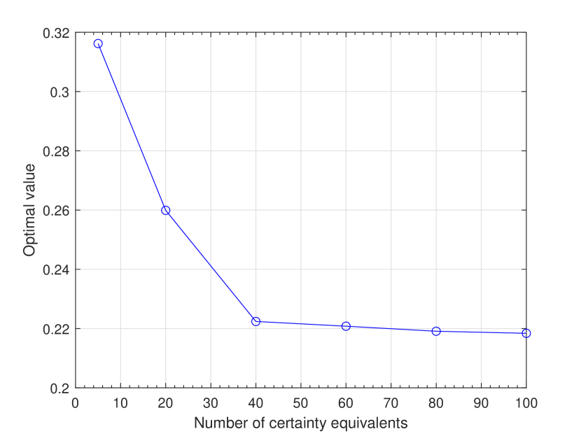
(b)

Figure 3: (a)Worst case value function vs increase of $K$.  (b) Change of $\rho_{{\cal V}_{El}\times{\cal W}_{r}}(\xi)$ in problem (5.3) vs increase of $K$.

Impact of ambiguity of the weighting functions

Figure 4 (a) depicts changes of the worst-case weighting function w.r.t. decrease of the radius while the number of pairwise comparisons is fixed at $M=5$ and the number of certainty equivalents is fixed at $K=5$. From the figure, we can see the convergence of the worst-case weighting functions to the true as $r$ reduces to $0$.

Figure 4 (b) displays the optimal values of PRGSR-CPT for the ambiguity sets $({\cal V}_{El},{\cal W}_{r})$. We can see that for the fixed number of pairwise comparisons, the PRGSR-CPT becomes smaller as the radius of ambiguity set decreases.

(a)

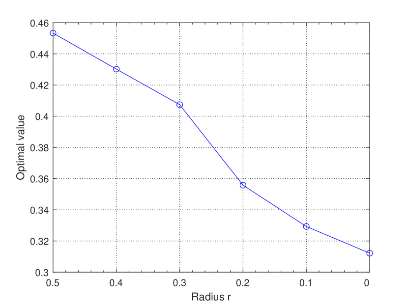
(b)

Figure 4: (a) Worst case weighting function vs decrease of $r$.  (b) Change of $\rho_{{\cal V}_{El}\times{\cal W}_{r}}(\xi)$ in problem (5.3) vs decrease of $r$.

The test results are consistent with our expectation that as more and more information about the DM’s preferences is obtained, the ambiguity of the true value function and weighting function reduces, the preference robust generalized shortfall risk converges to the true GSR-CPT.

6 Concluding remarks

In this paper, we explore Mao and Cai’s generalized shortfall risk measure when the value function and/or the weighting function are ambiguous. We introduce the concept of preference robust generalized shortfall risk measure which is based on a pair of the worst value function and weighting function from a joint ambiguity set value/weighting functions, investigate the properties of the robust generalized shortfall risk measure and develop computational algorithms for calculating the robust risk. The numerical tests show that the algorithms perform well w.r.t. increase of information about the DM’s risk preferences.

There are some limitations in the developed models and preference elicitation approaches. One is that the ambiguity set of the weighting functions is constructed through a ball centered at a nominal weighting function, it might be interesting to combine it with the pairwise comparison approach to reduce the ambiguity. This approach is expected to work well for each fixed value function but it seems to be challenging to elicit both the value function and the weighting function simultaneously. The other is that we are unable to use the CPT-based shortfall risk measure to represent the DM’s preference choice, rather we use the distorted expected values of prospects, that is, ${\mathbb{E}}[w_{-}w_{+}[v(\cdot)]$ to describe the DM’s pairwise choice. As discussed in Section 3.2, there could be a gap between the two approaches. Note also that in the numerical tests, instances of pairwise comparisons and certainty equivalents are generated randomly without any costs. In practice, eliciting a DM’s preferences in this manner may incur financial costs, see Vayanos et al. [32]. Thus it might be interesting to explore the idea as to how to optimally design questionnaires to elicit the true value/weighting functions using approaches such as [4]. We leave all these for future research.

Appendix Appendix A Supplementary materials

A.1 Properties of preference functional ${\mathbb{E}}_{w^{-}w^{+}}[v(\cdot)]$

Lemma A.1

Let ${\mathbb{E}}_{w^{-}w^{+}}[v(\zeta)]$ be defined as in (1.3). Then

$${\mathbb{E}}_{w^{-}w^{+}}[v(\eta)]\leq{\mathbb{E}}_{w^{-}w^{+}}[v(\xi)]\,\,\forall\eta,\xi\in{\cal L}^{0}({\rm I\!R})\mbox{\rm{ with }}\eta(\omega)\leq\xi(\omega),\forall\omega\in\Omega.$$ (A.1)

Proof. By definition (see (1.3)),

$${\mathbb{E}}_{w^{-}w^{+}}[v(\xi)]=\int_{0}^{\infty}w^{+}(\mathbb{P}(v(\xi)>t))dt+\int_{0}^{\infty}-w^{-}(\mathbb{P}(-v(\xi)>t))dt.$$

Since $\eta(\omega)\leq\xi(\omega)$ for all $\omega\in\Omega$ and $v(\cdot)$ is monotonically increasing, then $v(\eta(\omega))\leq v(\xi(\omega))$ for all $\omega\in\Omega$, and consequently

$$\mathbb{P}(v(\eta)>t)\leq\mathbb{P}(v(\xi)>t)\quad\mbox{\rm{and}}\quad\mathbb{P}(-v(\eta)>t)\geq\mathbb{P}(-v(\xi)>t).$$

Moreover, since $w^{-},w^{+}$ are strictly increasing, we have

$$w^{+}(\mathbb{P}(v(\eta)>t))\leq w^{+}(\mathbb{P}(v(\xi)>t))\quad\text{and}\quad-w^{-}(\mathbb{P}(-v(\eta)>t))\leq-w^{-}(\mathbb{P}(-v(\xi)>t)).$$

A combination of the inequalities give rise to

$${\mathbb{E}}_{w^{-}w^{+}}[v(\eta)]\leq{\mathbb{E}}_{w^{-}w^{+}}[v(\xi)].$$

The proof is complete.  

Lemma A.2

Let ${\mathbb{E}}_{w^{-}w^{+}}[v(\cdot)]$ be defined as in (1.3) and $\xi\in{\cal L}^{0}({\rm I\!R})$. Then the following assertions hold.

• For any $a,b\in{\rm I\!R}$ with $a\leq b$,

  $${\mathbb{E}}_{w^{-}w^{+}}[v(\xi-a)]\geq{\mathbb{E}}_{w^{-}w^{+}}[v(\xi-b)].$$ (A.2)

• For any $a,b\in{\rm I\!R}$ with $a<b$,

  $${\mathbb{E}}_{w^{-}w^{+}}[v(\xi-a)]>{\mathbb{E}}_{w^{-}w^{+}}[v(\xi-b)]\,\,\forall a<b.$$ (A.3)

Proof. Part (i) follows from directly from Lemma A.1.

Part(ii). Let $\Omega_{1}:=\{\omega\in\Omega:\xi(\omega)\leq b\}$. For real number $a\in{\rm I\!R}$, let $(a)_{+}:=\max\{a,0\}$ and $(a)_{-}:=\min\{a,0\}$. For any $a<b$, we have

$$\xi(\omega)-b<[\xi(\omega)-a]_{-},\forall\omega\in\Omega_{1}\quad\mbox{\rm{and}}\quad\xi(\omega)-b<[\xi(\omega)-a]_{+}\forall\omega\in\Omega\backslash{\Omega_{1}}.$$

Since the value function $v\in\mathscr{V}$ is strictly increasing, then

$$v^{-}(\xi(\omega-b))<v^{-}([\xi(\omega-a)]_{-}),\forall\omega\in\Omega_{1}\quad\mbox{\rm{and}}\quad v^{+}(\xi(\omega)-b)<v^{+}([\xi(\omega)-a]_{+}),\forall\omega\in\Omega\backslash{\Omega_{1}}.$$

Let

$$R_{1}:=\int_{\Omega_{1}}v^{-}(\xi(\omega)-b)\psi^{-}(\mathbb{P}(\{\tilde{\omega}\in\Omega:\xi(\tilde{\omega})\leq\xi(\omega)\}))d\mathbb{P}(\omega)$$

and

$$R_{2}:=\int_{\Omega\backslash{\Omega_{1}}}v^{+}(\xi(\omega)-b)\psi^{+}(1-\mathbb{P}(\{\tilde{\omega}\in\Omega:\xi(\tilde{\omega})\leq\xi(\omega)\}))d\mathbb{P}(\omega).$$

By the definition of ${\mathbb{E}}_{(v,w^{-},w^{+})}[v(\cdot)]$, we have

$${\mathbb{E}}_{w^{-}w^{+}}[v(\xi-b)] = \int_{\Omega_{1}}v^{-}(\xi(\omega)-b)\psi^{-}(\mathbb{P}(\{\tilde{\omega}\in\Omega:\xi(\tilde{\omega})\leq\xi(\omega)\}))d\mathbb{P}(\omega)$$

$$+\int_{\Omega\backslash{\Omega_{1}}}v^{+}(\xi(\omega)-b)\psi^{+}(1-\mathbb{P}(\{\tilde{\omega}\in\Omega:\xi(\tilde{\omega})\leq\xi(\omega)\}))d\mathbb{P}(\omega)$$

$$= R_{1}+R_{2}.$$

Since we have either $\mathbb{P}(\Omega_{1})>0$ or $\mathbb{P}(\Omega\backslash\Omega_{1})>0$ or both, then

$${\mathbb{E}}_{w^{-}w^{+}}[v(\xi-b)] < \int_{\Omega_{1}}v^{-}([\xi(\omega)-a]_{-})\psi^{-}(\mathbb{P}(\{\tilde{\omega}\in\Omega:\xi(\tilde{\omega})\leq\xi(\omega)\}))d\mathbb{P}(\omega)$$

$$+\int_{\Omega\backslash{\Omega_{1}}}v^{+}([\xi(\omega)-a]_{+})\psi^{+}(1-\mathbb{P}(\{\tilde{\omega}\in\Omega:\xi(\tilde{\omega})\leq\xi(\omega)\}))d\mathbb{P}(\omega)$$

$$= \int^{b}_{-\infty}v^{-}([u-a]_{-})\psi^{-}(F_{\xi}(u))dF_{\xi}(u)+\int^{\infty}_{b}v^{+}([u-a]_{+})\psi^{+}(1-F_{\xi}(u))dF_{\xi}(u)$$

$$\leq \int^{a}_{-\infty}v^{-}(u-a)\psi^{-}(F_{\xi}(u))dF_{\xi}(u)+\int^{\infty}_{a}v^{+}(u-a)\psi^{+}(1-F_{\xi}(u))dF_{\xi}(u)$$

$$= {\mathbb{E}}_{w^{-}w^{+}}[v(\xi-a)].$$

The proof is complete.  

A.2 Proof of Theorem 4.1

Proof. We divide the proof into four steps.

Step 1. By definition, we have

$$\sup_{(v,w^{-},w^{+})\in{\cal V}_{El}\times{\cal W}_{r}\times{\cal W}_{r}}\sum_{i=-m}^{n}\pi_{i}v(x-\xi_{i})=\sup_{v\in{\cal V}_{El}}\sup_{(w^{-},w^{+})\in{\cal W}_{r}\times{\cal W}_{r}}\sum_{i=-m}^{n}\pi_{i}v(x-\xi_{i}),$$

where ${\cal V}_{El}={\cal V}_{ce}^{K}\cap{\cal V}^{M}_{pair}\cap{\cal V}_{S}$ and ${\cal W}_{r}=B(w_{0},r)$. For each fixed $v\in{\cal V}_{El}$, let

$$\phi(v):=\sup_{(w^{-},w^{+})\in{\cal W}_{r}\times{\cal W}_{r}}\sum_{i=-m}^{n}\pi_{i}v(x-\xi_{i}).$$

Then $\sup_{(v,w^{-},w^{+})\in{\cal V}_{El}\times{\cal W}_{r}\times{\cal W}_{r}}\sum_{i=-m}^{n}\pi_{i}v(x-\xi_{i})=\sup_{v\in{\cal V}_{El}}\phi(v)$. It suffices to derive the tractable reformulation of $\phi(v)$ for each $v\in{\cal V}_{El}$.

Step 2. Let $q_{-m-1}=0,$ $q_{i}=\sum_{j=-m}^{i}p_{j}$ for $i=-m,\cdots,n$. We choose the set of breakpoints of the piecewise linear weighting functions such that it contains $q_{i},1-q_{i}$, i.e.,

$$\{q_{i}:i=-m-1,\cdots,-1\}\cup\{1-q_{i}:-1,\cdots,n\}\subset\{t_{1},\cdots,t_{T+1}\}.$$ (A.4)

Define the $\tilde{g}$-ball of piecewise linear inverse $S$-shaped weighting functions

centered at $w_{0}$ with radius $r$

$${\widetilde{B}}(w_{0},r):=\left\{w\in\mathscr{W}_{T}\cap{\mathscr{W}}_{inS}:\mathsf{d\kern-0.70007ptl}_{\tilde{g}}(w,w_{0})\leq r\right\}.$$ (A.5)

Denote by $\Psi(\psi^{0},r)$ the set of all derivative functions of $w\in B(w_{0},r)$, i.e.,

$$\Psi(\psi^{0},r):=\left\{\psi\in\Psi:w\in B(w_{0},r)\right\}=\left\{\psi\in\Psi:\displaystyle\sup_{g\in{\mathscr{G}}}\left|\int_{0}^{1}g(t)(\psi(t)-\psi^{0}(t))dt\right|\leq r\right\},$$

where $\Psi$ is the set of all derivative functions of $w\in{\mathscr{W}}_{inS}$ . Note that for $\psi\in\Psi(\psi^{0},r)$, it is not necessarily a step-like function. Thus we propose to use step-like functions with jump points at set $\{t_{2},\cdots,t_{T}\}$ to approximate it. Consequently we define

$${\widetilde{\Psi}}(\psi^{0},r)=\left\{\psi\in\Psi_{T}:\displaystyle\sup_{g\in{\mathscr{G}}}\left|\sum_{l=1}^{T}\int_{t_{l}}^{t_{l+1}}g(t)(\psi_{l}-\psi^{0}_{l})dt\right|\leq r\right\},$$ (A.6)

where $\Psi_{T}$ is defined as in (3.26). Since $\pi_{i}=w^{-}\left(q_{i}\right)-w^{-}\left(q_{i-1}\right),$ for $i=-m,\cdots,-1$, and $\pi_{i}=w^{+}\left(1-q_{i-1}\right)-w^{+}\left(1-q_{i}\right)$, for $i=0,1,\cdots,n$, we can write $\phi(v)$ as

$$\phi(v)=\sup_{(\psi^{-},\psi^{+})\in\Psi(\psi^{0},r)\times\Psi(\psi^{0},r)}\left\{\sum_{i=-m}^{-1}v^{-}(\xi_{i}-x)\int_{q_{i-1}}^{q_{i}}\psi^{-}(t)dt+\sum_{i=0}^{n}v^{+}(\xi_{i}-x)\int_{1-q_{i}}^{1-q_{i-1}}\psi^{+}(t)dt\right\}.\;\;$$ (A.7)

Next, we will prove that $\phi(v)$ is equal to

$$\widetilde{\phi}(v):=\sup_{(\psi^{-},\psi^{+})\in{\widetilde{\Psi}}(\psi^{0},r)\times{\widetilde{\Psi}}(\psi^{0},r)}\left\{\sum_{i=-m}^{-1}v^{-}(\xi_{i}-x)\int_{q_{i-1}}^{q_{i}}\psi^{-}(t)dt+\sum_{i=0}^{n}v^{+}(\xi_{i}-x)\int_{1-q_{i}}^{1-q_{i-1}}\psi^{+}(t)dt\right\}$$

for any $v\in{\cal V}_{El}$. Since ${\widetilde{B}}(w_{0},r)\subset B(w_{0},r)$, we have $\widetilde{\phi}(v)\leq\phi(v).$ It suffices to show that $\widetilde{\phi}(v)\geq\phi(v)$. Let $\varepsilon>0$, and $w^{*-}_{\varepsilon},w^{*+}_{\varepsilon}\in B(w_{0},r)$ be such that

$$\sum_{i=-m}^{-1}\left(w^{*-}_{\varepsilon}(q_{i})-w^{*-}_{\varepsilon}(q_{i-1})\right)v(\xi_{i}-x)+\sum_{i=0}^{n}\left(w^{*+}_{\varepsilon}(1-q_{i-1})-w^{*+}_{\varepsilon}(1-q_{i})\right)v(\xi_{i}-x)$$ (A.8)

$$\geq \sup_{(w^{-},w^{+})\in B(w_{0},r)\times B(w_{0},r)}\left\{\sum_{i=-m}^{-1}\left(w^{-}(q_{i})-w^{-}(q_{i-1})\right)v(\xi_{i}-x)\right.$$

$$\left.+\sum_{i=0}^{n}\left(w^{+}(1-q_{i-1})-w^{+}(1-q_{i})\right)v(\xi_{i}-x)\right\}-\varepsilon.$$

We can find piecewise linear functions $w^{*-}_{\varepsilon,T},w^{*+}_{\varepsilon,T}$ such that $w^{*-}_{\varepsilon,T}(t_{i})=w^{*-}_{\varepsilon}(t_{i})$ and $w^{*+}_{\varepsilon,T}(t_{i})=w^{*+}_{\varepsilon}(t_{i})$, $i=1,\cdots,T+1$,

$$w^{*-}_{\varepsilon,T}(t):=w^{*-}_{\varepsilon}(t_{i-1})+\frac{w^{*-}_{\varepsilon}(t_{i})-w^{*-}(t_{i-1})}{t_{i}-t_{i-1}}(t-t_{i-1}),\mbox{ for }t\in[t_{i-1},t_{i}],i=2,\cdots,T+1,$$

$$w^{*+}_{\varepsilon,T}(t):=w^{*+}_{\varepsilon}(t_{i-1})+\frac{w^{*+}_{\varepsilon}(t_{i})-w^{*+}(t_{i-1})}{t_{i}-t_{i-1}}(t-t_{i-1}),\mbox{ for }t\in[t_{i-1},t_{i}],i=2,\cdots,T+1.$$

For $w^{*-}_{\varepsilon},w^{*+}_{\varepsilon}\in B(w_{0},r)$, we have

$$\mathsf{d\kern-0.70007ptl}_{\tilde{g}}(w^{*-}_{\varepsilon},w_{0})=\sup_{g\in{\mathscr{G}}}\left|\int_{0}^{1}g(t)(\psi_{\varepsilon}^{-}(t)-\psi^{0}(t))dt\right|\leq r,$$

$$\mathsf{d\kern-0.70007ptl}_{\tilde{g}}(w^{*+}_{\varepsilon},w_{0})=\sup_{g\in{\mathscr{G}}}\left|\int_{0}^{1}g(t)(\psi_{\varepsilon}^{+}(t)-\psi^{0}(t))dt\right|\leq r.$$

Then

$$\mathsf{d\kern-0.70007ptl}_{\tilde{g}}(w^{*-}_{\varepsilon,T},w_{0})=\sup_{g\in{\mathscr{G}}}\left|\sum_{l=2}^{T+1}\int_{t_{l-1}}^{t_{l}}g(t)\left(\frac{w^{*-}_{\varepsilon}(t_{l})-w^{*-}(t_{l-1})}{t_{l}-t_{l-1}}-\psi^{0}_{l}\right)dt\right|=\mathsf{d\kern-0.70007ptl}_{\tilde{g}}(w^{*-}_{\varepsilon},w_{0})\leq r,$$

$$\mathsf{d\kern-0.70007ptl}_{\tilde{g}}(w^{*+}_{\varepsilon,T},w_{0})=\sup_{g\in{\mathscr{G}}}\left|\sum_{l=2}^{T+1}\int_{t_{l-1}}^{t_{l}}g(t)\left(\frac{w^{*+}_{\varepsilon}(t_{l})-w^{*+}(t_{l-1})}{t_{l}-t_{l-1}}-\psi^{0}_{l}\right)dt\right|=\mathsf{d\kern-0.70007ptl}_{\tilde{g}}(w^{*+}_{\varepsilon},w_{0})\leq r,$$

which means $w^{*-}_{\varepsilon},w^{*+}_{\varepsilon}\in{\widetilde{B}}(w_{0},r)$. Since $q_{i},1-q_{i}\in\{t_{1},\cdots,t_{T+1}\}$ in (A.4), then $w^{*-}_{\varepsilon,T}(q_{i})=w^{*-}_{\varepsilon}(q_{i})$, for $i=-m-1,\cdots,-1$, and $w^{*+}_{\varepsilon,T}(1-q_{i})=w^{*+}_{\varepsilon}(1-q_{i})$, for $i=0,\cdots,n$, and

$$\widetilde{\phi}(v) = \sup_{(w^{-},w^{+})\in{\widetilde{B}}(w_{0},r)\times{\widetilde{B}}(w_{0},r)}\left\{\sum_{i=-m}^{-1}\left(w^{-}_{\varepsilon}(q_{i})-w^{-}_{\varepsilon}(q_{i-1})\right)v(\xi_{i}-x)\right.$$

$$\left.+\sum_{i=0}^{n}\left(w^{+}_{\varepsilon}(1-q_{i-1})-w^{+}_{\varepsilon}(1-q_{i})\right)v(\xi_{i}-x)\right\}$$

$$\geq \sum_{i=-m}^{-1}\left(w^{*-}_{\varepsilon,T}(q_{i})-w^{*-}_{\varepsilon,T}(q_{i-1})\right)v(\xi_{i}-x)+\sum_{i=0}^{n}\left(w^{*+}_{\varepsilon,T}(1-q_{i-1})-w^{*+}_{\varepsilon,T}(1-q_{i})\right)v(\xi_{i}-x)$$

$$= \sum_{i=-m}^{-1}\left(w^{*-}_{\varepsilon}(q_{i})-w^{*-}_{\varepsilon}(q_{i-1})\right)v(\xi_{i}-x)+\sum_{i=0}^{n}\left(w^{*+}_{\varepsilon}(1-q_{i-1})-w^{*+}_{\varepsilon}(1-q_{i})\right)v(\xi_{i}-x)$$

$$\geq \sup_{(w^{-},w^{+})\in B(w_{0},r)\times B(w_{0},r)}\left\{\sum_{i=-m}^{-1}\left(w^{-}(q_{i})-w^{-}(q_{i-1})\right)v(\xi_{i}-x)\right.$$

$$\left.+\sum_{i=0}^{n}\left(w^{+}(1-q_{i-1})-w^{+}(1-q_{i})\right)v(\xi_{i}-x)\right\}-\varepsilon=\phi(v)-\varepsilon,$$

where the last inequality is due to (A.8). This means $\widetilde{\phi}(v)\geq\phi(v)$ since $\varepsilon$ can be arbitrarily small. This shows $\phi(v)=\widetilde{\phi}(v)$ as desired.

Step 3. Let $y_{i}:=\int_{t_{i}}^{t_{i+1}}g(t)dt$. Since ${\mathscr{G}}$ constitutes all measurable functions with $|g(t)|\leq\tilde{g}(t)$ for $t\in[0,1]$, then we have $|y_{i}|\leq\int_{t_{l}}^{t_{l+1}}\tilde{g}(t)dt$. The inequality in ${\widetilde{\Psi}}(\psi^{0},r)$ (A.6) can be reformulated as follows

$$\sup\limits_{g\in{\mathscr{G}}}\left|\sum_{l=1}^{T}\int_{t_{l}}^{t_{l+1}}g(t)(\psi_{l}-\psi^{0}_{l})dt\right| =\sup\limits_{y_{1},\cdots,y_{T}} \sum_{l=1}^{T}(\psi_{l}-\psi^{0}_{l})y_{l}$$ (A.9)

$${\rm s.t.} |y_{l}|\leq\int_{t_{l}}^{t_{l+1}}\tilde{g}(t)dt,\,l=1,\cdots,T.$$

The right hand side is a linear program. We derive its Lagrange dual. Let $\eta\in{\rm I\!R}^{T}_{+}$ and $\theta\in{\rm I\!R}^{T}_{+}$ denote the dual variables corresponding to constraints $-y_{l}\leq\int_{t_{l}}^{t_{l+1}}\tilde{g}(t)dt$ for $l=1,\cdots,T$ and $y_{l}\leq\int_{t_{l}}^{t_{l+1}}\tilde{g}(t)dt$ for $l=1,\cdots,T$ respectively. Let

$$L(y;\eta,\theta) := \sum_{l=1}^{T}(\psi_{l}-\psi^{0}_{l})y_{l}-\sum_{l=1}^{T}\eta_{l}\left(-y_{l}-\int_{t_{l}}^{t_{l+1}}\tilde{g}(t)dt\right)-\sum_{l=1}^{T}\theta_{l}\left(y_{l}-\int_{t_{l}}^{t_{l+1}}\tilde{g}(t)dt\right)$$

$$= \sum_{l=1}^{T}\left(\psi_{l}-\psi^{0}_{l}+\eta_{l}-\theta_{l}\right)y_{l}+\sum_{l=1}^{T}\eta_{l}\int_{t_{l}}^{t_{l+1}}\tilde{g}(t)dt+\sum_{l=1}^{T}\theta_{l}\int_{t_{l}}^{t_{l+1}}\tilde{g}(t)dt.$$

The Lagrange dual can be written as

$$\inf\limits_{\eta,\theta\geq 0} \sum_{l=1}^{T}(\eta_{l}+\theta_{l})\int_{t_{l}}^{t_{l+1}}\tilde{g}(t)dt$$

$${\rm s.t.} \psi_{l}-\psi^{0}_{l}+\eta_{l}-\theta_{l}=0,l=1,\cdots,T.$$

Thus $\phi(v)$ in (A.7) can be reformulated as

$$\phi(v) = \sup_{(\psi^{-},\psi^{+})\in{\widetilde{\Psi}}(\psi^{0},r)\times{\widetilde{\Psi}}(\psi^{0},r)}\left\{\sum_{i=-m}^{-1}v^{-}(\xi_{i}-x)\int_{q_{i-1}}^{q_{i}}\psi^{-}(t)dt+\sum_{i=0}^{n}v^{+}(\xi_{i}-x)\int_{1-q_{i}}^{1-q_{i-1}}\psi^{+}(t)dt\right\}$$ (A.10)

$$= \sup_{\tilde{\psi}^{-},\tilde{\psi}^{+},\eta,\theta}\sum_{i=-m}^{-1}v^{-}(\xi_{i}-x)\sum_{l=1}^{T}\psi_{l}^{-}\int_{q_{i-1}}^{q_{i}}\mathds{1}_{[t_{l},t_{l+1})}(t)dt+\sum_{i=0}^{n}v^{+}(\xi_{i}-x)\sum_{l=1}^{T}\psi^{+}_{l}\int_{1-q_{i}}^{1-q_{i-1}}\mathds{1}_{[t_{l},t_{l+1})}(t)dt$$

$$\quad{\rm s.t.}\quad(\ref{robust_Wra})-(\ref{robust_Wrj}),$$

where $\tilde{\psi}^{-}=(\psi^{-}_{l},\cdots,\psi^{-}_{T})$ and $\tilde{\psi}^{+}=(\psi^{+}_{l},\cdots,\psi^{+}_{T})$.

Step 4. We are now ready to reformulate the constraint function in (4.8)

$$\sup_{(v,w^{-},w^{+})\in({\cal V}_{El},{\cal W}_{r},{\cal W}_{r})}\sum_{i=-m}^{n}\pi_{i}v(\xi_{i}-x)=\sup_{v\in{\cal V}_{El}}\phi(v).$$

First, we will prove

$$\sup_{v\in{\cal V}_{El}}\phi(v)=\sup_{v\in{\cal{\widetilde{V}}}_{El}}\phi(v),$$ (A.11)

where ${\cal{\widetilde{V}}}_{El}$ is defined as follows.

Let $\{y_{j}\}_{j=1}^{J}$ be the $j$-th entry of ranked support set $\mathscr{S}:=\bigcup_{m=1}^{M}({\rm supp}(\gamma_{m})\cup{\rm supp}(\eta_{m}))\cup\{a,b\}\cup\{0\}\cup\bigcup_{i=1}^{N}(\xi_{i}-x)\cup\bigcup_{k=1}^{K}{\rm supp}(A_{k}-a_{k}^{+})\cup\bigcup_{k=1}^{K}{\rm supp}(A_{k}-a_{k}^{-})$. We will use $y_{j}$ to denote the $j$-th smallest entry of $\mathscr{S}$. Let $j_{0}$ be the index satisfying $y_{j_{0}}=0$. Denote

$$\mathscr{\tilde{V}}:=\left\{v:[\alpha,\beta]\rightarrow{\rm I\!R}\;:\begin{array}[]{ll}&v\mbox{\rm{ is negative and convex on $[\alpha,0)$, and positive and concave on $(0,\beta]$}}\\ &v\mbox{\rm{ is increasing continuous, }}v(\alpha)=b_{l},v(\beta)=b_{r}\end{array}\right\}.$$

Let $\mathscr{\tilde{V}}_{J}$ denote the set of all piecewise linear functions $v\in\mathscr{\tilde{V}}$ with breakpoints $a=y_{1}<y_{2}<\cdots<y_{J}=b$, $y_{1},\cdots,y_{J}\in\mathscr{S}$. For

$${\cal V}_{El}={\cal V}^{K}_{ce}\cap{\cal V}^{M}_{pair}\cap{\cal V}_{S}=\left\{v\in{\mathscr{\tilde{V}}}:\begin{array}[]{ll}&\mathbb{E}_{w^{-}w^{+}}[v(\gamma_{m})]\leq\mathbb{E}_{w^{-}w^{+}}[v(\eta_{m})],m=1,\cdots,M\\ &{\mathbb{E}}_{w^{-}w^{+}}[v(A_{k}-a_{k}^{+})]\leq 0,k=1,\cdots,K\\ &{\mathbb{E}}_{w^{-}w^{+}}[v(A_{k}-a_{k}^{-})]\geq 0,k=1,\cdots,K\end{array}\right\},$$

we define the ambiguity set

$${\cal{\widetilde{V}}}_{El}={\cal V}^{K}_{ce,J}\cap{\cal V}^{M}_{pair,J}\cap{\cal V}_{S}=\left\{v_{J}\in\mathscr{\tilde{V}}_{J}:\begin{array}[]{ll}&\mathbb{E}_{w^{-}w^{+}}[v_{J}(\gamma_{m})]\leq\mathbb{E}_{w^{-}w^{+}}[v_{J}(\eta_{m})],m=1,\cdots,M\\ &{\mathbb{E}}_{w^{-}w^{+}}[v_{J}(A_{k}-a_{k}^{+})]\leq 0,k=1,\cdots,K\\ &{\mathbb{E}}_{w^{-}w^{+}}[v_{J}(A_{k}-a_{k}^{-})]\geq 0,k=1,\cdots,K\end{array}\right\}.$$

We consider to approximate ${\cal V}_{El}$ by ${\cal{\widetilde{V}}}_{El}$. The approximation function $v_{J}\in\mathscr{\tilde{V}}_{J}$ preserves convexity, concavity and increasing property, and then $\mathscr{\tilde{V}}_{J}\subset\mathscr{\tilde{V}}$. We choose $\gamma_{m}$ and $\eta_{m}$, $m=1,\cdots,M$ with discrete distributions, and the breakpoints cover their support sets. Since

$${\mathbb{E}}_{w^{-}w^{+}}[v(\xi)] = \int_{0}^{\infty}w^{+}(\mathbb{P}(v(\xi)\geq t))dt-\int_{-\infty}^{0}w^{-}(\mathbb{P}(v(\xi)\leq t))dt$$

$$= \int_{0}^{\infty}w^{+}(1-F_{\xi}(t))dv^{+}(t)-\int_{-\infty}^{0}w^{-}(F_{\xi}(t))dv^{-}(t),$$

then

$$\mathbb{E}_{w^{-}w^{+}}[v_{J}(\gamma_{m})]-\mathbb{E}_{w^{-}w^{+}}[v_{J}(\eta_{m})] = \int_{y_{1}}^{y_{J}}\phi_{m}(y)dv_{J}(y)=\sum_{i=1}^{J-1}\phi_{m}(y_{j})\Big{(}v_{J}(y_{i+1})-v_{J}(y_{i})\Big{)}$$

$$= \sum_{i=1}^{J-1}\phi_{m}(y_{j})\Big{(}v(y_{i+1})-v(y_{i})\Big{)}=\mathbb{E}_{w^{-}w^{+}}[v(\gamma_{m})]-\mathbb{E}_{w^{-}w^{+}}[v(\eta_{k})],$$

where $\phi_{m}$ is defined as in (5.19).

$${\mathbb{E}}_{w^{-}w^{+}}[v_{J}(A_{k}-a_{k}^{+})]$$

$$= \int_{y_{j_{0}}}^{y_{J}}w^{+}(1-F_{A_{k}-a_{k}^{+}}(y))dv_{J}^{+}(y)-\int_{y_{1}}^{y_{j_{0}}}w^{-}(F_{A_{k}-a_{k}^{+}}(y))dv_{J}^{-}(y)$$

$$= \sum_{j={j_{0}}}^{J-1}w^{+}(1-F_{A_{k}-a_{k}^{+}}(y_{j}))\Big{(}v_{J}^{+}(y_{j+1})-v_{J}^{+}(y_{j})\Big{)}-\sum_{j=1}^{{j_{0}}-1}w^{-}(F_{A_{k}-a_{k}^{+}}(y_{j}))\Big{(}v_{J}^{-}(y_{j+1})-v_{J}^{-}(y_{j})\Big{)}$$

$$= \mathbb{E}_{w^{-}w^{+}}[v(A_{k}-a_{k}^{+})]$$

and

$${\mathbb{E}}_{w^{-}w^{+}}[v_{J}(A_{k}-a_{k}^{-})]$$

$$= \int_{y_{j_{0}}}^{y_{J}}w^{+}(1-F_{A_{k}-a_{k}^{-}}(y))dv_{J}^{+}(y)-\int_{y_{1}}^{y_{j_{0}}}w^{-}(F_{A_{k}-a_{k}^{-}}(y))dv_{J}^{-}(y)$$

$$= \sum_{j={j_{0}}}^{J-1}w^{+}(1-F_{A_{k}-a_{k}^{-}}(y_{j}))\Big{(}v_{J}^{+}(y_{j+1})-v_{J}^{+}(y_{j})\Big{)}-\sum_{j=1}^{{j_{0}}-1}w^{-}(F_{A_{k}-a_{k}^{-}}(y_{j}))\Big{(}v_{J}^{-}(y_{j+1})-v_{J}^{-}(y_{j})\Big{)}$$

$$= \mathbb{E}_{w^{-}w^{+}}[v(A_{k}-a_{k}^{-})].$$

This shows ${\cal{\widetilde{V}}}_{El}\subset{\cal V}_{El}$, and hence $\displaystyle\sup_{v\in{\cal{\widetilde{V}}}_{El}}\phi(v)\leq\sup_{v\in{\cal V}_{El}}\phi(v)$. Conversely, let $\varepsilon>0$, and $v_{\varepsilon}^{*}\in{\cal V}_{El}$ such that

$$\phi(v_{\varepsilon}^{*})\geq\sup_{v\in{\cal V}_{El}}\phi(v)-\varepsilon.$$

We can find a piecewise linear function $v_{\varepsilon,J}^{*}\in{\cal{\widetilde{V}}}_{El}$ such that $v^{*}_{\varepsilon,J}(\xi_{i}-x)=v^{*}_{\varepsilon}(\xi_{i}-x)$ for $1\leq i\leq N$. Specifically, for any $v\in{\cal V}_{El}$, we can construct such a $v_{J}$ as

$$v_{J}(y):=v(y_{i-1})+\frac{v(y_{i})-v(y_{i-1})}{y_{i}-y_{i-1}}(y-y_{i}),\mbox{ for }y\in[y_{i-1},y_{i}],i=2,\cdots,J,$$

where $y_{1}=a,y_{J}=b$. Observe that $v_{J}$ satisfies $v_{J}(y_{i})=v(y_{i})$ for each $i$. Consequently we have

$$\sup_{v\in{\cal{\widetilde{V}}}_{El}}\phi(v)\geq\phi(v^{*}_{\varepsilon,J})=\phi(v^{*}_{\varepsilon})\geq\sup_{v\in{\cal V}_{El}}\phi(v)-\varepsilon.$$

Then $\sup_{v\in{\cal{\widetilde{V}}}_{El}}\phi(v)\geq\sup_{v\in{\cal V}_{El}}\phi(v)$ follows as $\varepsilon$ can be arbitrarily small, and thus (A.11) holds.

Next, by invoking (A.10), we can reformulate the constraint function in (4.8) as

$$\sup_{(v,w^{-},w^{+})\in{\cal V}_{El}\times{\cal W}_{r}\times{\cal W}_{r}}\sum_{i=-m}^{n}\pi_{i}v(\xi_{i}-x)=\sup_{v\in{\cal V}_{El}}\phi(v)$$

$$= \sup_{v\in{\cal{\widetilde{V}}}_{El}}\sup_{\tilde{\psi}^{-},\tilde{\psi}^{+},\eta,\theta}\sum_{i=-m}^{-1}v^{-}(\xi_{i}-x)\sum_{l=1}^{T}\psi_{l}^{-}\int_{q_{i-1}}^{q_{i}}\mathds{1}_{[t_{l},t_{l+1})}(t)dt+\sum_{i=0}^{n}v^{+}(\xi_{i}-x)\sum_{l=1}^{T}\psi^{+}_{l}\int_{1-q_{i}}^{1-q_{i-1}}\mathds{1}_{[t_{l},t_{l+1})}(t)dt$$

$$\qquad\qquad{\rm s.t.}\qquad(\ref{robust_Wra})-(\ref{robust_Wrj}),$$

$$= \sup_{a,b}\sup_{\tilde{\psi}^{-},\tilde{\psi}^{+},\eta,\theta}\left\{\sum_{i=-m}^{-1}\Big{(}(a_{1}(\xi_{i}-x)+b_{1})\mathds{1}_{(-\infty,0)\cap[y_{1},y_{2}]}(\xi_{i}-x)\right.$$

$$\qquad\qquad\qquad+\sum_{j=2}^{J-1}(a_{j}(\xi_{i}-x)+b_{j})\mathds{1}_{(-\infty,0)\cap(y_{j},y_{j+1}]}(\xi_{i}-x)\Big{)}\sum_{l=1}^{T}\psi_{l}^{-}\int_{q_{i-1}}^{q_{i}}\mathds{1}_{[t_{l},t_{l+1})}(t)dt$$

$$\qquad\qquad\qquad+\sum_{i=0}^{n}\Big{(}(a_{1}(\xi_{i}-x)+b_{1})\mathds{1}_{(-\infty,0)\cap[y_{1},y_{2}]}(\xi_{i}-x)$$

$$\left.\qquad\qquad\qquad+\sum_{j=2}^{J-1}(a_{j}(\xi_{i}-x)+b_{j})\mathds{1}_{(-\infty,0)\cap(y_{j},y_{j+1}]}(\xi_{i}-x)\Big{)}\sum_{l=1}^{T}\psi^{+}_{l}\int_{1-q_{i}}^{1-q_{i-1}}\mathds{1}_{[t_{l},t_{l+1})}(t)dt\right\}$$

$$\qquad\qquad{\rm s.t.}\qquad(\ref{robust_Wra})-(\ref{robust_Wrj}),~{}~{}~{}(\ref{robust_v_ob})-(\ref{robust_v_oj}).$$ (A.13a)

The proof is complete.

References

- [1] C. Acerbi, Spectral measures of risk: A coherent representation of subjective risk aversion. Journal of Banking Finance, 26: 1505-1518, 2002.
- [2] M. Allais, Le comportement de l’homme rationnel devant le risque: critique des postulats et axiomes de l’école américaine. Econometrica: Journal of the Econometric Society, 21: 503-546, 1953.
- [3] B. Armbruster and E. Delage, Decision making under uncertainty when preference information is incomplete. Management science, 61: 111-128, 2015.
- [4] D. Bertsimas and A. O’Hair, Learning preferences under noise and loss aversion: An optimization approach, Operations Research, 61: 1190–1199, 2013.
- [5] H. Bühlmann, Mathematical Methods in Risk Theory. Springer, Berlin, 1970.
- [6] H. Bühlmann, Premium calculation from top down. ASTIN Bulletin: The Journal of the IAA, 15: 89-101, 1985.
- [7] J. Cai, J. Li and T. Mao, Distributionally robust optimization under distorted expectations. Available at SSRN 3566708, 2020.
- [8] R.T. Clemen and T. Reilly, Making Hard Decisions with Decision Tools Suite. 2nd ed. Duxbury, Pacific Grove, CA, 2001.
- [9] D.R. Cavagnaro, M.A. Pitt, R. Gonzalez and J.I. Myung, Discriminating among probability weighting functions using adaptive design optimization. Journal of risk and uncertainty, 47: 255-289, 2013.
- [10] G.B. Davies and S.E. Satchell, The behavioural components of risk aversion. Journal of Mathematical Psychology, 51: 1-13, 2007.
- [11] E. Delage, S. Guo and H. Xu, Shortfall risk models when information of loss function is incomplete, 2018.
- [12] D. Denneberg, Premium calculation: why standard deviation should be replaced by absolute deviation. ASTIN Bulletin: The Journal of the IAA, 20: 181-190, 1990.
- [13] D. Ellsberg, Risk, ambiguity, and the savage axioms. The quarterly journal of economics, 75: 643–669, 1961.
- [14] D.D. Escobar and G.C. Pflug, The distortion principle for insurance pricing: properties, identification and robustness. Annals of Operations Research, 292: 771–794, 2018.
- [15] H. Föllmer and A. Schied, Convex measures of risk and trading constraints. Finance and stochastics, 6: 429-447, 2002.
- [16] H. Föllmer and A. Schied, Stochastic Finance. An Introduction in Discrete Time. 2nd ed., Berlin: De Gruyter, 2004.
- [17] K. Giesecke, T. Schmidt and S. Weber, Measuring the risk of large losses. Journal of Investment Management, 6: 1-15, 2008.
- [18] S. Guo and H. Xu, Distributionally robust shortfall risk optimization model and its approximation. Mathematical Programming, 174: 473-498, 2019.
- [19] S. Guo and H. Xu, Utility Preference Robust Optimization with Moment-Type Information Structure. Optimization Online, 2021.
- [20] B. Haskell, L. Fu and M. Dessouky, Ambiguity in risk preferences in robust stochastic optimization. European Journal of Operational Research, 254: 214-225, 2016.
- [21] S. Heilpern, A rank-dependent generalization of zero utility principle. Insurance: Mathematics and Economics, 33: 67–73, 2003.
- [22] J. Hu and S. Mehrotra, Robust decision making over a set of random targets or risk-averse utilities with an application to portfolio optimization. IIE Transactions, 47: 358-372, 2015.
- [23] J. Hu and G. Stepanyan, Optimization with reference-based robust preference constraints. SIAM Journal on Optimization, 27: 2230-2257, 2017.
- [24] D. Kahneman and A. Tversky, Prospect theory: an analysis of decision under risk, Econometrica, 47: 263–291, 1979.
- [25] M. Kaluszka and M. Krzeszowiec, Pricing insurance contracts under cumulative prospect theory. Insurance: Mathematics and Economics, 50: 159-166, 2012.
- [26] U.S. Karmarkar, Subjectively weighted utility: A descriptive extension of the expected utility model. Organizational behavior and human performance, 21: 61-72, 1978.
- [27] U.S. Karmarkar, Subjectively weighted utility and the Allais paradox. Organizational Behavior and Human Performance, 24: 67-72, 1979.
- [28] A. Kothiyal, V. Spinu and P.P. Wakker, Prospect theory for continuous distributions: A preference foundation. Journal of risk and uncertainty, 42: 195, 2011.
- [29] T. Mao and J. Cai, Risk measures based on behavioural economics theory. Finance and Stochastics, 22: 367-393, 2018.
- [30] M. Nardon and P. Pianca, Insurance premium calculation under continuous cumulative prospect theory. University Ca’Foscari of Venice, Dept. of Economics Research Paper Series No. 3, 2019.
- [31] J. von Neumann and O. Morgenstern, Theory of games and economic behavior. Bulletin American Mathematical Society, 51: 498-504, 1945.
- [32] P. Vayanos, Y. Ye, D. McElfresh, J. Dickerson, E. Rice, Robust active preference elicitation, arXiv:2003.01899, 2020.
- [33] S.M. Pesenti, Q. Wang and R. Wang, Optimizing distortion riskmetrics with distributional uncertainty. Available at SSRN, 2020.
- [34] D. Prelec, The probability weighting function. Econometrica, 497-527, 1998.
- [35] J. Quiggin, A theory of anticipated utility. Journal of Economic Behavior Organization, 3: 323-343, 1982.
- [36] J. Quiggin, Generalized expected utility theory: The rank-dependent model. Springer Science & Business Media, 2012.
- [37] J.W. Tuthill and D.L. Frechette, Non-expected utility theories: Weighted expected, rank dependent, and cumulative prospect theory utility. No. 1266-2016-101906, 2002.
- [38] A. Tversky and D. Kahneman, Advances in prospect theory: Cumulative representation of uncertainty. Journal of Risk and uncertainty, 5: 297-323, 1992.
- [39] W. Wang and H. Xu, Preference robust distortion risk measure and its application. Available at SSRN: http://dx.doi.org/10.2139/ssrn.3763632
- [40] W. Wang and H. Xu, Robust spectral risk optimization when information on risk spectrum is incomplete. SIAM Journal on Optimization, 30: 3198-3229, 2020.
- [41] P. Wakker and A. Tversky, An axiomatization of cumulative prospect theory. Journal of risk and uncertainty, 7: 147-175, 1993.
- [42] S. Weber, Distribution‐invariant risk measures, information, and dynamic consistency. Mathematical Finance: An International Journal of Mathematics, Statistics and Financial Economics, 16: 419-441, 2006.
- [43] S. Zhang and H. Xu, Generalized shortfall risk measure based on insurance premium. Available at SSRN: http://dx.doi.org/10.2139/ssrn.3819088, 2021.